the e conomic c ase for hs 2assets.hs2.org.uk/sites/default/files/inserts/s&a 1_economic...
TRANSCRIPT

The economic case For hs2
October 2013

The economic case For hs2
October 2013

High Speed Two (HS2) Limited has been tasked by the Department for Transport (DfT) with managing the delivery of a new national high speed rail network. It is a non-departmental public body wholly owned by the DfT.
High Speed Two (HS2) Limited,2nd Floor, Eland House,Bressenden Place,London SW1E 5DU
Telephone: 020 7944 4908
General email enquiries: [email protected]
Website: www.hs2.org.uk
High Speed Two (HS2) Limited has actively considered the needs of blind and partially sighted people in accessing this document. The text will be made available in full on the HS2 website. The text may be freely downloaded and translated by individuals or organisations for conversion into other accessible formats. If you have other needs in this regard please contact High Speed Two (HS2) Limited.
© High Speed Two (HS2) Limited, 2013, except where otherwise stated.
Copyright in the typographical arrangement rests with High Speed Two (HS2) Limited.
This information is licensed under the Open Government Licence v2.0. To view this licence, visit www.nationalarchives.gov.uk/doc/open-government-licence/version/2 or write to the Information Policy Team, The National Archives, Kew, London TW9 4DU, or e-mail: [email protected]. Where we have identified any third-party copyright information you will need to obtain permission from the copyright holders concerned.
Document code: S&A 1
Printed in Great Britain on paper containing at least 75% recycled fibre.

Economic Case for HS2
1
Contents
Preface 5
1 Executive summary 7
1.1 Overview 7
1.2 The standard approach to economic appraisal 8
1.3 The potential for higher returns 11
1.4 The impact on economic geography 15
2 Introduction 17
2.1 Scope and purpose of this document 17
2.2 Document structure 17
3 Changes to our analytical framework 19
3.1 Overview 19
3.2 Updates to our approach 19
4 Standard case results 23
4.1 Introduction 23
4.2 Projecting benefits and costs into the future 23
4.3 Risk versus uncertainty analysis 25
4.4 Standard case risk analysis 26
4.5 Conclusions 29
5 Impact of long-term demand growth 30
5.1 Introduction 30
5.2 Recent growth 30
5.3 Variability in demand growth 32
5.4 Demand cap 32
5.5 Demand cap with risk analysis 33
5.6 Impact of fares on demand and interaction with the demand cap 38
5.7 Differential fares and the impact of competition 41
5.8 Conclusions 42
6 Monetary valuation of time savings 43

Economic Case for HS2
2
6.1 The value of time in appraisal 43
6.2 Value of time scenario tests 45
6.3 Results from value of time scenarios 45
7 Construction and operating costs 49
7.1 Introduction 49
7.2 Construction costs 49
7.3 Operating costs 52
8 Beyond conventional appraisal 54
8.1 Limitations of our economic appraisal 54
8.2 The limits to the standard approach for calculating benefits 60
8.3 The impact of non-linearities in demand relationships 61
8.4 The impact of fixed land-use patterns 62
Appendices 64
1 Modelling and appraisal approach 64
1.1 PLANET modelling 64
1.2 Updates to our approach 65
2 Scheme assumptions and service patterns 69
2.1 Phase One 69
2.2 Phase Two and the full network 69
2.3 HS2 service patterns 69
2.4 Released capacity service patterns 69
2.5 Freight 70
3 Cost assumptions 73
3.1 Overview 73
3.2 Construction costs 73
3.3 Rolling stock costs 74
3.4 Infrastructure and rolling stock renewals 75
3.5 Quantified Risk Assessment 76
3.6 Operating costs 76
4 Calculation of the BCR 79
4.2 Description of benefits 79
4.3 Costs and revenue 80
4.4 Calculation of the BCR 81
5 Transport impacts for the standard case 82
5.1 Benefits breakdown 82
5.2 Where passengers come from 82
5.3 Regional benefits 83
6 Scenario results 84
6.2 Standard case 85

Economic Case for HS2
3
6.3 Higher demand cap – Demand cap 10% higher 86
6.4 WebTAG 2012 value of time 87
6.5 Alternative value of time 88
6.6 Construction cost target price scenario 90
6.7 The ‘V-network’ 91
7 Glossary 92
List of figures
Figure 1: Benefit cost ratio results for the full network using standard appraisal 10
Figure 2: Benefit cost ratio results for Phase One only using standard appraisal 11
Figure 3: Three graphs demonstrating the sensitivity of BCR outcomes to different demand caps 13
Figure 4: Benefits cost ratio results with alternative value of time 15
Figure 5: Costs and benefits as they are incurred over the life of HS2 24
Figure 6: Results of analysis for full network BCR 27
Figure 7: Long run average GDP per capita growth rates: historic versus risk analysis assumptions 28
Figure 8: Results of analysis of Phase One only 29
Figure 9: Graph showing long-distance transport trends from 1995 to 2012 31
Figure 10: Recent trend for growth in journeys on long distance operators services compared to our forecast for future rail journeys over 100 miles without HS2 32
Figure 11: Results from increasing the demand cap by 10% 34
Figure 12: Impact on the BCR of increasing the demand cap by 39% 35
Figure 13: Impact on the BCR of decreasing the demand cap by 20% 36
Figure 14: Different assumptions about how the rate of demand growth might decline 37
Figure 15: Results on the BCR of demand growth assumptions applied in the aviation industry 38
Figure 16: Results on the BCR of assuming lower future rail fares 39
Figure 17: Benefit cost ratio results with low fare and high demand assumptions 40
Figure 18: Benefit cost ratio results with high fare and high demand assumptions 41
Figure 19: Benefit cost ratio results with alternative value of time assumptions 48
Figure 20: Benefit cost ratio results with low value of time assumptions 48
Figure 21: Risk analysis results for Phase One under three different assumptions 50
Figure 22: Risk analysis results for the full network under two different assumptions 51
Figure 23: Results for the full network of varying the level of optimism bias for the operating costs 53
Figure 24: Changes in economic output (£, 2013 prices) after investment in HS2 – conurbations on the HS2 network 57
Figure 25: The potential for mis-estimation of benefits from the rule of a half 61
Figure 26: Illustration of staged approach to calculating benefits 62
Figure 27: HS2 Phase One service pattern 71
Figure 28: HS2 full network service pattern 72
Economic Case for HS2
4
List of tables
Table 1: Variables examined through risk analysis and scenario tests 26
Table 2: Forecast annual ‘Do Minimum’ rail trips per household over 100 miles 35
Table 3: Changes in value of time used in WebTAG (2010 prices) 43
Table 4: Values of time used in scenarios (2010 prices) 46
Table 5: Varying construction costs for each Phase dependant on the amount of risk included 49
Table 6: How the KPMG report and the HS2 economic case vary in their analysis of the economic impact of HS2 network 59
Table 7: Breakdown of base construction costs (excluding risk allowances) 2011 prices 74
Table 8: Breakdown of rolling stock costs (2011 prices) 75
Table 9: Breakdown of operating costs (2011 prices present value including Optimism Bias) 78
Table 10: Grouped and disaggregated benefits, what they are and where they are calculated 80
Table 11: Total net benefits including WEIs for standard case 82
Table 12: Breakdown of where passengers will be generated from 83
Table 13: Regional distribution of transport user benefits (value in brackets are in £millions) 83
Table 14: Parameters uses in each of the scenario tests 84
Table 15: Economic analysis results for the standard case scenario (2011 PV) 85
Table 16: Scenario results for a 10% higher demand cap 86
Table 17: Changes in value of time used in WebTAG (2010 prices) 87
Table 18: WebTAG 2012 value of time scenario 87
Table 19: Values of time used to value benefits from the long distance model 88
Table 20: Values of time used to value benefits from PFM regional (short distance) models 89
Table 21: Scenario results for an alternative value of time 89
Table 22: Economic analysis results for the target price scenario 90
Table 23: Results for the V-network, Phase Two given Phase One 91

Economic Case for HS2
5
Preface This document presents our advice to the Government on the economic case for HS2. It is one of a suite of documents that are being published today to set out the case for investing in the HS2 railway. It should be read in conjunction with the strategic case, which summarises the full rationale for the scheme.
The economic case analysis has been carried out in accordance with HM Treasury’s The Green Book and DfT’s transport analysis guidance (WebTAG). In line with that guidance, our analytical framework is based on ‘social cost benefit analysis’, and as such it attempts to place a monetary value on as many impacts as possible. However, the economic case can only ever provide part of the overall picture, and there are many other factors that can and should be taken into account.
The WebTAG analysis approach has been developed and refined over several years to
encapsulate best practice and provide a common basis for the comparison of proposals. In order to provide that common basis, some simplifying assumptions and approximations are provided within the guidance.
HS2 is an unusual proposal in many respects. It is both national in scale, and yet it strongly impacts on existing transport networks at a local level. It is a transformational scheme which:
connects 8 out of 10 of the major cities in the UK;
almost doubles capacity on north-south inter-city routes; and
offers step-changes in journey times.
HS2 pushes at the boundaries of standard appraisal practice.
HS2 will have significant impacts on behaviour, with implications for future land-use patterns,
particularly around its stations. This is significant because it is not possible with conventional transport appraisal approaches to capture the potential benefits of changes in businesses and households’ location in response to the scheme. The new connections and opportunities generated by HS2 (including over 20 million new long distance trips per year) will change markets and create opportunities for increased trade, which may lead to a redistribution and specialisation of economic activity across the UK. As a first step in gaining a greater understanding of these issues, we have commissioned research to develop a methodological framework to analyse the potential scale and distribution of these regional impacts. The initial findings are reported as part of the evidence base in this report.
However, even this new research has only examined the potential implications for the distribution of economic activity within the UK. Evidence1 shows that the quality of transport links is an important factor in international companies’ locations. Improving our transport infrastructure will help to attract multinational companies to the UK, resulting in increased investment and increased economic growth. Research to gain a better understanding of this effect will form part of our future analytical work programme.
1 European Cities Monitor (2010), p4: http://www.europeancitiesmonitor.eu/wp-content/uploads/2010/10/ECM-2010-Full-Version.pdf

Economic Case for HS2
6
Other significant aspects of the scheme relating to step-changes in track capacity are also difficult
to capture with cost benefit analysis.
Analysis in the strategic case explains how the resilience of the current network could be improved by investing in HS2. Whilst we capture the higher reliability of high-speed services on the HS2 network in the economic case, our modelling does not reflect the reductions in delays that could be achieved by relieving the pressure on the rest of network. In the context of a congested network, where the knock-on delays from any given incident are typically increasing, this is a significant issue for rail users.
In a broader sense, the additional track capacity, which will form an integral part of the nation’s transport networks, will also provide us with the flexibility to accommodate a range of patterns of economic growth. By connecting 8 of the 10 major cities of the UK with a high-speed network and releasing significant amounts of capacity on the conventional network, HS2 will open up a vast
number of options for rail service patterns. We have modelled just one of these options here, but we have not captured the additional value of the adaptability that the investment creates.
We will continue to gather further evidence on these impacts, as well as keeping our cost benefit
analysis up to date, to provide as broad an evidence base as possible in support of the case for action. The case will continue to evolve as our detailed understanding of the potential of the scheme improves.

Economic Case for HS2
7
1 Executive summary 1.1 Overview
1.1.1 This document presents an analysis of the economic case for High Speed Two (HS2). It is the first substantive update to the analysis since January 2012 and constitutes our current view on the strength of the economic case for the HS2 network. This new analysis has benefited from a comprehensive programme of work to further enhance our analytical tools, which has significantly improved our ability to forecast and appraise the impacts of HS2. On this basis we believe it to be the best representation of the economic case for HS2 to date.
1.1.2 We have timed the delivery of this analysis to support the Government’s decision on whether to proceed with the deposit of a Hybrid Bill to permit the construction of
Phase One (between London and the West Midlands), and to inform the Government’s consultation on the line of route for Phase Two (from the West Midlands to Manchester, Leeds and beyond. We therefore report results for both the Phase One proposal, and the HS2 network as a whole.
1.1.3 HS2 will be one of the largest public infrastructure projects ever undertaken in the UK and will have long-lasting implications for how people will travel and how businesses will trade. It will add much-needed additional track capacity to the north-south routes of our railway system, creating opportunities to improve the frequency and reliability of rail services for towns and cities, both on and off the HS2 network.
1.1.4 The substantial reductions in journey times delivered by HS2 will have the potential to change the very economic geography of the country. The integration of the additional
track capacity with the rest of the rail network will provide far greater flexibility in how we can use our rail infrastructure, and leave us better able to adapt to future needs as required.
1.1.5 HS2 is a large undertaking, with significant upfront capital investment, but also benefits that will accrue for generations to come. The sheer size of the project, and the longevity of its impacts, magnifies the opportunities and risks of investment. It is not possible to forecast far into the future without some degree of uncertainty, and we have therefore focused our analysis on understanding the range of possible outcomes, rather than simply providing a single benefit cost ratio (BCR).
1.1.6 Most of our analysis is carried out in line with the Department for Transport’s (DfT) standard cost-benefit analysis framework as set out in the published guidance2. In the course of preparing our analysis it has become clear that some of the standard
assumptions and approximations provided in the guidance are exerting a strong influence on results. To illustrate this, we have presented scenarios that demonstrate the impact of alternative assumptions.
2WebTAG is the Department for Transport’s guidance on how to assess the costs and benefits of transport infrastructure/policies. WebTAG sets out the methods and assumptions that the DfT recommends should be used to model the impact of schemes. http://www.dft.gov.uk/webtag/

Economic Case for HS2
8
1.1.7 Furthermore, some aspects of the scheme are simply not amenable to analysis with
the DfT’s standard cost-benefit analysis techniques. For instance, our economic appraisal holds land-use patterns fixed. Given the transformational nature of the improvements that will be delivered by HS2, it seems inconceivable that there will be no changes in behaviour that will affect future patterns of land use. This means the standard approach may be missing some important economic productivity impacts from the scheme.
1.1.8 Over the past year we have invested considerable effort in developing new analytical tools to examine how HS2 might affect productivity. We present some results from our first work in this area, and recommend that they are considered as a complement to the economic case for the scheme.
1.1.9 On the basis of our analysis, we have reached three main conclusions:
The standard cost-benefit analysis shows that the benefits of the HS2 network exceed the costs by a considerable margin and that under standard assumptions the economic cases for both phases of the project are robust and are resilient to a wide range of factors and events.
Standard assumptions on the demand cap and the value of time (VoT) in the appraisal fail to capture large amounts of potential additional benefits from HS2. There is a significant chance that the return on investment in HS2 could be considerably higher than previous appraisals have suggested.
HS2 has the potential to deliver productivity gains that will alter geographic
distribution of economic activity in a way that cannot be modelled in our economic appraisal. We recommend that the results of the impacts on economic geography are considered alongside the results from the standard appraisal.
1.2 The standard approach to economic appraisal
1.2.1 Guidance on how to assess the costs and benefits of transport infrastructure projects is set out in DfT’s appraisal guidance. As part of this analysis, the costs and benefits are compared against each other to generate a ‘benefit-cost ratio’: i.e. the value of benefits that would result from every £1 that the scheme costs.
1.2.2 The assessment captures the costs, benefits and changes in revenues for the whole of the rail network – not just those associated with the HS2 infrastructure. This includes the costs of both constructing and operating the railway. The benefits include lower levels of overcrowding, on both HS2 and existing services, and quicker, more frequent and more reliable journeys for passengers. These costs and benefits are appraised
over a 67 year period for the full network from 2026 (the opening of Phase One) to 2092 (60 years after the opening of Phase Two).
1.2.3 Since August 2012, we have significantly enhanced our analytical tools. The PLANET Framework Model (PFM), which provides forecasts of demand, travel patterns, and crowding levels, has been updated using more recent input assumptions, better evidence and improved techniques. We have improved our understanding of operating costs, and we have reviewed and improved our treatment of optimism bias. Construction costs have been updated, and for Phase One a full quantified risk

Economic Case for HS2
9
assessment of costs is now used to inform our analysis. Our analysis is also based on
the new, lower business values of time that have been issued in WebTAG for use from next year.
1.2.4 Some of these changes, for instance, our improved understanding of business use of the rail network, have increased benefit cost ratios. Others, for example, reductions in the business value of time and increases in constructions costs, have lowered benefit cost ratios. Although the impacts of some of the individual changes have been significant, the overall net impact of all of the changes taken together has been minimal.
1.2.5 We have also further developed our approach to allow us to illustrate the impact of uncertainty around long-term economic growth, construction costs, demand forecasting and values of time on returns from the investment. We are now able to
present a distribution of benefit cost ratios, rather than just a single point estimate, and illustrate the impact of different factors on the strength of the economic case.
1.2.6 Using the standard approach, the point-estimate BCR of the whole network (including
Wider Economic Impacts) is estimated at 2.3. Importantly, Figure 1 sets out the results of our analysis on the distribution of benefit cost ratios generated by considering the combined impact of the uncertainty around some of the key drivers3 of value for money (VfM).
3 The variables examined as part of the risk analysis are: short and long term economic growth, construction costs, how demand responds to changes in GDP and fares, the value placed on time-savings by leisure travellers and commuters and how sensitive this value is to economic growth. The risk analysis therefore covers a significant range of possible outcomes, however, it is not possible to cover every eventuality.

Economic Case for HS2
10
Figure 1: Benefit cost ratio results for the full network using standard appraisal
1.2.7 The distribution has been mapped against the Department for Transport’s value for money categories to allow comparison with other schemes. On the basis of the factors analysed here, the full HS2 network is expected to offer ‘High’ value for money. More than 75% of the benefit cost ratios in the analysis are higher than 2 i.e. offering a return of more than £2 for every £1 invested.
1.2.8 The lowest benefit cost ratios, on the left-hand side of the distribution, are consistent with a pessimistic view of the world – high construction costs combined with low economic growth, lower values of time and low growth in demand.
1.2.9 Economic growth exerts a strong influence over the value for money of the scheme as it affects the likely rate of growth in demand, and therefore revenues, and also the valuation that is placed on some of the benefits of the scheme.
1.2.10 The distribution above incorporates the impact of a wide range of economic growth assumptions. Even with historically low levels of growth, enduring for many decades, under this analysis the scheme would still most likely offer medium value for money.
1.2.11 Figure 2 shows the same analysis for Phase One. The standard approach generates an
estimate of the BCR, with wider economic impacts, of 1.7, and our risk analysis shows a high likelihood, greater than 75%, of Phase One being medium value for money or higher. Low economic growth increases the risk of Phase One becoming low value for money, but on the basis of the variables analysed here, the risk of the scheme being poor value for money is negligible.
0%
5%
10%
15%
20%
25%
30%
35%
40%
45%
0.5 to 0.75 0.75 to 1 1 to 1.25 1.25 to 1.5 1.5 to 1.75 1.75 to 2 2 to 2.25 2.25 to 2.5 2.5 to 2.75 Beyond2.75
Like
liho
od
Benefit-Cost Ratio including WEIs
Standard appraisal: Distribution of Benefit-Cost Ratios for the full network
'Poor' Value for Money
'Low' Value for Money
'Medium' Value for Money
'High' Value for Money
0% of sample 1% of sample 20.3% of sample 78.7% of sample

Economic Case for HS2
11
Figure 2: Benefit cost ratio results for Phase One only using standard appraisal
1.2.12 We have included a wide range of construction costs in our analyses, from the target price that HS2 Ltd has been set for Phase One (£17.1 billion 2011 prices) to the highest estimate of cost including the maximum level of contingency (£21.2 billion 2011 prices)4. These conclusions are therefore resilient to a range of assumptions about cost contingency. However, lower levels of contingency are clearly associated with
higher value for money which is why HS2 Ltd is determined to deliver the project within the target price set for the company as part of the spending review. Maintaining a vigorous and disciplined approach to cost control is a key priority.
1.3 The potential for higher returns
1.3.1 From our analysis of the value for money of HS2, it is clear that some of the standard assumptions and approximations that are provided in the DfT guidance are exerting a strong influence over the results of the cost benefit analysis. In particular, our analysis suggests that the hard limit that is placed on the growth in demand and revenues by the guidance, and the use of values of time that do not vary with length of journey, are leading to a significant underestimation of the benefits that could be realised from the investment in HS2.
1.3.2 The conventional approach to handling the uncertainty around long-term growth in the demand for travel is to cap the demand for travel at a pre-determined year in the future. In the cost benefit analysis, growth in demand is assumed to halt abruptly and no account is taken of the potential for further growth in revenues or the volume of benefits after that point. For the appraisal of HS2, that level of demand has been set
4 Both sets of figures quoted here exclude sunk costs for appraisal purposes in line with WebTAG 3.5.9.
0%
5%
10%
15%
20%
25%
30%
35%
40%
45%
0.5 to 0.75 0.75 to 1 1 to 1.25 1.25 to 1.5 1.5 to 1.75 1.75 to 2 2 to 2.25 2.25 to 2.5 2.5 to 2.75 Beyond2.75
Like
liho
od
Benefit-Cost Ratio including WEIs
Standard appraisal: Distribution of Benefit-Cost Ratios for Phase 1
'Poor' Value for Money
'Low' Value for Money
'Medium' Value for Money
'High' Value for Money
0.5% of sample 23% of sample 65% of sample 11.6% of sample

Economic Case for HS2
12
to be consistent with previous appraisals. This is now 2036 – only three years after the
opening of Phase Two. This means that for the remaining 57 years of the appraisal, demand is held constant at 2036 levels irrespective of future growth in population or GDP.
1.3.3 While it would be unreasonable to expect demand for rail travel to continue growing indefinitely, our view is that this assumption is probably conservative, and that the standard practice of conducting analysis for only one level of demand cap obscures the potential for much higher returns from further growth in demand.
1.3.4 The series of graphs in Figure 3 show that modest changes to the demand cap can lead to significant changes in the benefit cost ratios, with much higher likelihoods of the scheme being high or even very high (BCR>4) value for money. Setting the cap at a higher level would result in the cap level being reached later than 2036.
1.3.5 A 10% increase in that level results in the cap being reached in 2040 with a point estimate BCR of 2.8 and a very high probability of the BCR being in the high or very high value for money categories. A 39% increase results in the cap being reached in
2049 with a point estimate BCR of 4.5 and an even higher probability of the BCR being in the high or very high categories. Under these longer-term demand growth scenarios the point-estimate BCR lies between 2.8 and 4.5.
0%
10%
20%
30%
40%
50%
60%
Like
liho
od
Full network - BCR with WEIs (ratio) 2011 Prices/PV
Standard Case
'Poor' VfM
'Low' VfM
'Medium' VfM
'High' VfM
0%of sample
1%of sample
20.3%of sample
78.7%of sample
'Very high' VfM
0%of sample

Economic Case for HS2
13
Figure 3: Three graphs demonstrating the sensitivity of BCR outcomes to different demand caps
1.3.6 Another assumption, which we think is leading to a significant understatement of benefits from HS2, is the practice of using a single value of time for all lengths of trip in the appraisal. Many studies over the years have demonstrated that people are willing to pay far more for time savings when making long journeys – the very
0%
10%
20%
30%
40%
50%
60%
Like
liho
od
Full network - BCR with WEIs (ratio) 2011 Prices/PV
Demand growth stops at 2040
'Poor' VfM
'Low' VfM
'Medium' VfM
'High' VfM
0%of sample
0.2%of sample
3.7%of sample
95.2%of sample
'Very high' VfM
1%of sample
0%
10%
20%
30%
40%
50%
60%
Like
liho
od
Full network - BCR with WEIs (ratio) 2011 Prices/PV
Demand growth stops at 2049
'Poor' VfM
'Low' VfM
'Medium' VfM
'High' VfM
0%of sample
0%of sample
0.4%of sample
33.8%of sample
'Very high' VfM
65.9%of sample

Economic Case for HS2
14
journeys that the HS2 network would serve. This effect is not reflected in the standard appraisal.
1.3.7 There are a number of factors that may contribute to this effect, including business travellers’ desire to make long-distance trips and spend more time with their clients without having to stay overnight, and the greater probability of being able to do something useful with the larger time savings offered by high speed rail. That is not to say that business travellers do not try to make best use of their time whilst travelling, rather that businesses have a clear preference for not having their most productive staff stuck in transit.
1.3.8 In their report Valuation of Travel Time Savings for Business Travellers5, the Institute for Transport Studies (ITS) at Leeds University reported that the evidence for high-speed rail supports “a business valuation in excess of the wage rate. Indeed, across the
central values for each study, the value of time was on average around 50% larger than the gross wage rate, and across the six UK studies it was 40% larger”.
1.3.9 We have conducted a test to illustrate the impact on the BCR of adopting alternative
values of time as suggested by the ITS Leeds research. The test uses a business value of time of £45 per hour (2010 prices), this is 40% higher than the newly updated values of time of £32 per hour (2010 prices) but still lower than the value used in the August 2012 economic update (£47 per hour). The test also uses non-business values of time that have been adjusted to better reflect the length of trips that are affected by HS2 and other modelled changes in service patterns.
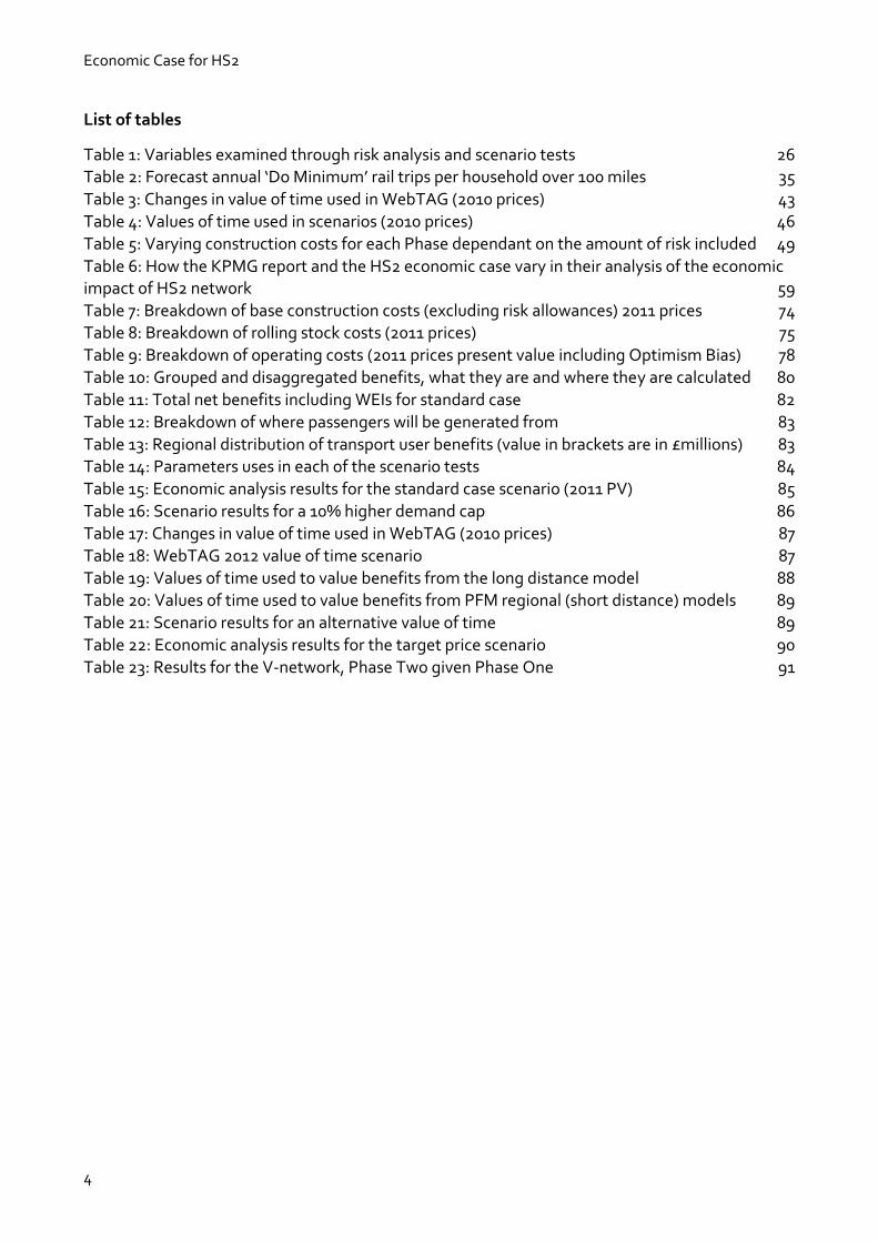
1.3.10 Figure 4 shows that the adoption of these values of travel time, based on a higher willingness-to-pay, would lead to significantly different conclusions about the risks to the return on the investment. Under these assumptions, HS2 delivers a return that is
greater than £2 for every £1 invested in virtually all of the tested scenarios - even those with the most pessimistic economic growth, cost and demand forecasting assumptions.
5 Valuation of Travel Time Savings for Business Travellers - (Transport appraisal and strategic modelling website) - www.gov.uk/government/collections/transport-appraisal-and-strategic-modelling-tasm-research-reports
Economic Case for HS2
15
Figure 4: Benefits cost ratio results with alternative value of time
1.4 The impact on economic geography
1.4.1 Our analysis demonstrates that investment in HS2 offers strong returns that are resilient to a broad range of eventualities and risks around costs, demand growth and the performance of the economy. We have conducted this analysis in accordance with
the DfT guidance on cost benefit analysis in order to provide a basis for comparison with alternative options and proposals.
1.4.2 However, when drawing comparisons with other schemes it is important to recognise that our economic appraisal may not fully capture the full range of potential benefits from investment in a transformational scheme such as HS2.
1.4.3 HS2 will lead to greater opportunities for businesses and people in one area to connect with businesses and people in other areas. This is true for city regions benefitting directly from HS2 services, but also for areas which benefit from released capacity on the classic network. Greater opportunities to connect with others make these areas more attractive places for businesses and people to locate. We would expect people and businesses to take these new opportunities into account in their
location decisions, and that this could ultimately lead to changes in future patterns of land use. The impact of such changes in land-use is not captured in our standard cost benefit analysis.
0%
5%
10%
15%
20%
25%
30%
35%
40%
Like
liho
od
Full network - BCR with WEIs (ratio) 2011 Prices/PV
Higher willingness to pay for long journeys
'Poor' VfM
'Low' VfM
'Medium' VfM
'High' Value for Money
0%of sample
0%of sample
0.6%of sample
95.1%of sample
'Very high' VfM
4.3%of sample
Economic Case for HS2
16
1.4.4 In order to understand the potential opportunity created as a result of investment in
HS2, we commissioned separate analysis6 to examine regional economic impacts measured in terms of productivity. The analysis approaches the question of economic impact in a different way to our appraisal, but is well grounded in economic theory, and considers the impact that investment in HS2 would have on economic output by understanding how such investment would influence regional economic performance, both in terms of overall economic productivity and, crucially, the location of economic activity.
1.4.5 The results suggest that HS2 could boost the economy by as much as £15bn per year and concludes that it could be the regions – not London as some have suggested – that will be the biggest winners from the new rail line. There is some uncertainty over the importance of rail connectivity for productivity, but sensitivity tests using more cautious assumptions still show a substantial annual productivity boost of £ 8bn.
1.4.6 This is early work and it is difficult to draw a direct comparison between the results of the new analysis and our economic appraisal. Fundamental differences in methodological approach mean that it is not possible to directly compare results (and they are not additive), but this work suggests that there may be additional benefits from HS2 that are not being captured in our economic appraisal. We recommend that further work is done to consider whether the standard approach to appraisal can be developed further to capture a fuller integrated understanding of these impacts on economic geography.
6 HS2: The Regional Economic Impact (KPMG) - http://www.kpmg.com/uk/en/issuesandinsights/articlespublications/pages/hs2-regional-economic-impact.aspx

Economic Case for HS2
17
2 Introduction 2.1 Scope and purpose of this document
2.1.1 This document sets out HS2 Ltd's advice to the Government on the economic case for HS2. It is published alongside and in support of DfT’s strategic case, which summarises the case for action and the full rationale for the scheme.
2.1.2 This economic case focuses on the HS2 option and, using the standard guidance, analyses the potential value for money of the proposed HS2 scheme. It does not consider the value for money of alternatives; this is considered as part of DfT’s Strategic Case.
2.2 Document structure
2.2.1 This document is structured as follows:
Chapter 3 gives a brief overview of what has changed and been updated in the modelling framework;
Chapter 4 reports our analysis using the standard approach and assumptions. All the results are reported within a framework of risk analysis
Chapter 5 looks at the impact that the demand cap has on the case and how allowing for longer term demand growth might affect the BCR;
Chapter 6 discusses the value of time and the impact of alternative scenarios for the value of time on the case;
Chapter 7 looks in more detail at the impact of construction and operating costs on the value for money;
Chapter 8 summarises some of the limitations of the standard approach
particularly around land-use and economic geography and sets out the results of early work in this area;
Appendix 1 sets out the modelling approach and what has changed in the PFM model;
Appendix 2 sets out HS2 scheme assumptions and service patterns;
Appendix 3 has more detail on cost assumptions;
Appendix 4 sets out more detail on benefits and the calculation of the BCR;
Appendix 5 reports transport impacts from the standard case; and
Appendix 6 reports point estimate BCRs for the following scenarios:
Standard Case
10% higher demand cap
WebTAG 2012 values of time
Economic Case for HS2
18
Alternative values of time
Construction costs target price
Standard case for Phase Two of the scheme, assuming that Phase One is in place.
Supporting documentation
2.2.2 For more information on certain aspects of the analysis the economic case should be read in conjunction with other reports. These include:
Cost and risk status report
PLANET Framework Model (PFM V4.3) – Model Description
Risk analysis for the HS2 economic case – Technical documentation
Summary of Key Changes to the Economic Case Since August 2012
PFM v4.3: Assumptions report
PLANET Framework Model Audit Report

Economic Case for HS2
19
3 Changes to our analytical framework 3.1 Overview
3.1.1 The previous economic update was published in August 2012. This followed the more detailed economic case for HS2 published in January 2012. We have continued to review and update our economic assessment, refining our processes as we learn more about the project and the impact it will have on the UK.
3.1.2 In the time since the last publication we have conducted a comprehensive programme of development work on the modelling approach and methodology. We have responded to challenges to our analysis and significantly improved our methodology and assumptions for assessing the economic case for HS2. We have also been able to react to changing external factors, such as GDP forecasts, and internal factors, such as more detailed development of the design.
3.1.3 In line with advice from the National Audit Office (NAO) we have moved away from simply presenting our results as a single point estimate of the BCR. By presenting the
risks and uncertainties around the case we are better able to demonstrate the key factors and assumptions that our analysis is sensitive to, and more clearly address the risks that are being considered.
3.2 Updates to our approach
3.2.1 This section summarises the key changes we have made to our analysis. Updates have been made in most areas and more detail is available in the appendices to this document and a number of supporting documents: Cost and risk status report, PLANET framework model (PFM v4.3) – Model Description, Summary of Key Changes to the Economic Case Since August 2012.
Changes to route and design
3.2.2 The capital costs reflect the design that will support the Phase One Environmental Statement and the Phase Two line of route currently out for consultation. Two of the main changes since August 2012 are the inclusion of Manchester Airport and the exclusion of the Heathrow Spur to reflect the paused decision on the Heathrow spur whilst the Airports Commission conducts its review.
Revised demand forecasts
Our forecast of the number of passengers expected to travel on HS2 is a critical 3.2.3element of the economic case. Since August 2012 we have updated our approach to forecasting demand in order to incorporate:
revised assumptions on economic growth from the Office of Budget Responsibility (OBR). These impact the future forecasts of both demand and values of time;
revised assumptions on other drivers of rail demand such as employment,
population and the cost and time of travelling by other modes; and

Economic Case for HS2
20
the latest evidence on how rail demand changes in response to economic
growth as set out in WebTAG guidance and the Passenger Demand Forecasting Handbook version 5 (PDFH5).
Updates and improvements to appraisal
Furthermore, the Department for Transport has made a number of changes to its 3.2.4WebTAG guidance, which we have incorporated into our appraisal calculations. These include:
Revised value of time. The DfT have, alongside this report, published new
values of time (VoT) in draft WebTAG guidance for use in transport analysis. We have adopted the new draft values in anticipation. This reduces benefits attributable to business travellers but increases the benefits attributable to commuting and leisure passengers. The method by which VoT is grown over
time has also been revised. VoT is one of the key factors in our analysis and is explored in more detail in Chapter 5.
Costs and benefits are presented in 2011 prices using the Office of National
Statistics (ONS) GDP deflator as a measure of inflation. The ONS definition of this deflator has been changed from being more consistent with a Retail Price Index (RPI) to being more consistent with a Consumer Price Index (CPI) metric. As fares increase in line with RPI, this means that in real terms, our RPI+1% fares assumption results in increased revenue.
3.2.5 We have also made a number of other changes to bring our modelling more closely in line with WebTAG guidance including:
Business crowding and boarding or interchange impacts are now assessed
using business values of time rather than commuting values of time.
Consumer surplus calculations are now being undertaken at a more detailed level in the model to bring them more closely in line with the guidance.
Updates to the modelling approach
The transport impacts in the economic case continue to be forecast by a computer 3.2.6model called the PLANET Framework Model (PFM). Updates and enhancements to the model, and the evidence underpinning it, have improved its ability to accurately forecast how HS2 will be used. These updates include:
An improved evidence base from the National Travel Survey (NTS) which the
model uses to determine how passengers will react to the new journey
opportunities resulting from HS2. The model is now better able to reflect observed behaviour;
Improvements in understanding the accessibility of stations that ensures we are consistent in our assumptions on the provision of local transport schemes with organisations such as Transport for London (TfL);
An improved understanding of the categorisation of trips into business, leisure and commuting purposes. Analysis has shown that our previous categorisation

Economic Case for HS2
21
of trips using ticket types had failed to keep pace with changes in ticket
purchasing habits. The model is therefore now using the National Rail Travel Survey (NRTS) data to estimate journey purposes at a more disaggregated level; and
Our understanding of how rail passengers respond to travelling in crowded
conditions now follows the advice set out in the PDFH5 and adopted by the Department for Transport into the WebTAG guidance. These new assumptions take into account the amount of standing space as well as the amount of sitting space in train carriages.
Updates to the ‘without scheme’ baseline
The ‘without scheme’ (or ‘Do-Minimum’) baseline against which HS2 is compared has 3.2.7been updated with relevant schemes specified as part of the High Level Output
Specification covering the period 2014 - 2019 and some electrification that is expected to take place after 2020. It now reflects the electrification of the Midland Mainline, inclusion of additional InterCity Express Rolling Stock on the East Coast Mainline,
improvements to the West Coast Mainline timetable, the Northern Hub Scheme and the East-West scheme between Oxford and Milton Keynes.
Improved service patterns
There have been changes to the representation of HS2 service patterns in our model 3.2.8and also the released capacity service patterns. We have reviewed the HS2 services in light of our increased understanding of operational issues and risks, and also changes to the model, which have affected the level of demand to longer distance locations.
In terms of the HS2 service pattern for the Full Network, we have: 3.2.9
revised a service which in previous specifications served Birmingham and
Liverpool. This is now separated into two single services. To accommodate this
change we have made revisions to the services on the eastern leg by combining the York and a Leeds service into a service which splits at Meadowhall.
added some calls on one of the services to Scotland and Newcastle; and
removed the services to Heathrow, but retained the two paths for future use to reflect that consideration of the Heathrow spur is currently paused, while the Airports Commission conducts its review.
The Phase One service pattern has seen more substantial changes to ensure greater 3.2.10continuity between the two phases of the scheme. This has involved the removal of the peak service to Birmingham and the alignment of the stops on the Liverpool, Preston and Scottish services with those in the Full Network service pattern. Appendix 2 details the service pattern that we have adopted for HS2 in the modelling.
We have also incorporated updates to the train service patterns that are expected to 3.2.11run on the classic rail network before HS2 is built. This has led us to re-visit some of the released capacity service pattern assumptions.

Economic Case for HS2
22
It should be noted that this represents just one possible set of assumptions for 3.2.12business case modelling purposes and should not be interpreted as a proposed service specification. There are many other potential combinations of released capacity. Much more work will be needed to determine the ultimate train service specification that will actually be in operation when HS2 opens. The current set of assumptions that have been used for the modelling are set out in PFM v4.3: Assumptions report.
Improved cost estimation
The capital costs used in the analysis are consistent with the Government’s spending 3.2.13review announcement in June 2013, with one exception of rolling stock costs, where further cost refinement, undertaken since the Spending Review, has led to a reduction in costs.
These construction cost estimates are now derived with full use of quantified risk 3.2.14assessment.
Our operating cost assumptions have also undergone a major review with 3.2.15improvements to base cost estimates, changes to optimism bias on HS2 costs and the removal of optimism bias on any classic line savings.
Use of risk analysis
In putting together this report we have made extensive use of risk analysis to improve 3.2.16our understanding of risks to the value for money of the scheme. In line with National Audit Office recommendations, we have moved away from simply reporting a single point estimate BCR to reporting probabilities and distributions for a number of scenarios. More detail on the risk analysis is set out in Risk analysis for the HS2 economic case – Technical documentation.
Economic Case for HS2
23
4 Standard case results 4.1 Introduction
4.1.1 Our previous assessments of the economic case have focused on the production of single point-estimate BCRs, each based on a single set of outputs from the PFM model. We referred to this as our ‘central case’ and, in effect, it constituted the BCR for the scheme when following standard procedures and assumptions, as set out in the WebTAG guidance.
4.1.2 However, whilst this approach provides a basis for comparison, it is ultimately only one view of the future, and in an infrastructure project with a potential lifespan of over 100 years, a single point-estimate fails to capture the potential upside and downside risks to returns from the investment.
4.1.3 For this update of the economic case, we have adopted a different approach to assessing the strength of the case, which is based on assessing the potential range of returns in a way that allows us to understand the resilience of the case to a range of different futures.
4.2 Projecting benefits and costs into the future
4.2.1 HS2 is a large undertaking, with significant upfront capital investment, but also benefits that will accrue for generations to come. In order to capture the majority of the benefits from the scheme, cost and benefit streams are projected far out into the future. In our appraisal, in line with WebTAG guidance, the benefits and costs are projected out to a point 60 years after the opening of Phase Two i.e.20927.
4.2.2 The assumptions that are made when producing these projections, such as the rate of growth in demand for rail travel, and the strength of economic growth, can exert a strong influence on the results of the analysis.
4.2.3 This can be seen in Figure 5, which plots discounted projections of costs, benefits and revenue streams from the current day to the end of the appraisal period. The up-front capital investment is shown with the green/blue area underneath the central axis, with operating costs shown with the adjacent orange/blue area, which stretches to the
right. The benefit and revenue streams in the analysis, which only start once the railway is in operation, are represented with the red, blue and purple areas above the central axis.
4.2.4 Assumptions about how quickly rail demand will grow, and the point at which demand is assumed to stop growing in the cost benefit analysis, heavily influence the size of
the projected returns. In the standard analysis, depicted in Figure 5, demand is assumed to stop growing in 2036 (marked with an arrow), just three years after the opening of Phase Two, and hence the volumes of revenues and benefits grow no further beyond that point.
7 In theory, the residual value of the track and rolling stock in 2092 should be calculated and added to the appraisal. Given the difficulties of doing this, this additional benefit is currently excluded from our analysis.

Economic Case for HS2
24
Figure 5: Costs and benefits as they are incurred over the life of HS2
-4
-3
-2
-1
0
1
2
3
4
2013201520172019202120232025202720292031203320352037203920412043204520472049205120532055205720592061206320652067206920712073207520772079208120832085208720892091
Pres
ent v
alue
201
1 pr
ices
(£)
Billi
ons
Phase 2 OPEX
Phase 1 OPEX
Phase 2 CAPEX
Phase 1 CAPEX
Revenue
Transport User Benefits (Other)
Transport User Benefits (Business)
nb. excluding Wider Economic impacts
Demand cap in standard case

Economic Case for HS2
25
4.2.5 In order to inform the assessment of the resilience of the economic case we have
tested the strength of the case under a wide range of different assumptions, and with different methods for projecting benefits into the future.
4.3 Risk versus uncertainty analysis
4.3.1 When projecting costs and benefits into the future, assumptions have to be made about a number of unknowns. There are unknowns about future levels of demand, people’s future willingness to pay for high speed rail travel, and hence revenues. There are also risks in the build, construction and estimation of costs.
4.3.2 In this document unknowns have been classified into ‘risks’ and ‘uncertainties’.
4.3.3 The term ‘risk’ is used for unknowns for which it is possible to derive a statistically robust understanding of the likelihood of different values occurring. For example, the
Office of Budget Responsibility produces a short run central estimate of growth which we use for the standard point-estimate of the BCR. In addition, they also produce a range of different GDP outcomes over the next five years; and attach their best understanding of likelihood to those different outcomes over that period.
4.3.4 Where the likelihood of different values can be quantified in this way, we have used established statistical techniques to analyse the impact of many of these factors, acting together, on the returns to the investment, and hence determine the likelihood of different levels of return.
4.3.5 This approach relies on the definition of probability distributions of possible values for key factors, and the repeated simulation of the impact of different combinations of those factors on the outcomes in question. A key advantage of using such an approach is that it guards against excessive weight being placed on extreme outcomes that would require the coincidence of a set of unlikely events to occur.
4.3.6 For our analysis, ‘uncertainties’ are defined as unknowns for which there is not a
statistically based understanding of the likelihood of different values occurring. In some instances this may because there is no statistically robust evidence, in other instances there may be competing theories on how a value should be derived.
4.3.7 For this update to the Economic Case, such uncertainties have been analysed as discrete scenarios, and for each scenario, a risk analysis is conducted to give a distribution of outcomes.
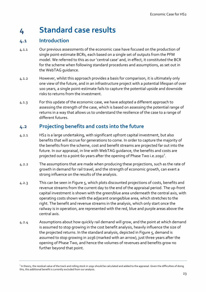
4.3.8 Table 1 sets out the key factors that have been analysed with a) risk analysis and b) scenario tests.
Economic Case for HS2
26
Variables explored as part of risk analysis Variables explored through alternative scenarios
Short and long-term economic growth (GDP) which feeds
into:
projections of demand and revenue; and
valuation of time-savings and other impacts.
When and/or at what level the growth in long-distance
rail demand should be capped.
The value placed on time savings by leisure travellers and
commuters.
The value placed on time savings by businesses.
The sensitivity of demand projections to economic growth
and level of fares.
Uncertainty about estimates of future operating costs.
How sensitive leisure and commuter traveller’s valuation of
time is to the growth in GDP.
Rail fares assumptions for the network.
Construction costs for Phase One and Phase Two using the
Quantified Risk Assessment work undertaken by HS2 Ltd.
Table 1: Variables examined through risk analysis and scenario tests
4.3.9 Values and distributions for these variables can be found in the supporting report: Risk analysis for the HS2 economic case – Technical documentation.
4.3.10 The rest of this chapter presents the results of the risk analysis for the standard case. Chapters 5, 6 and 7 present results for alternative scenarios, each reflecting a different source of uncertainty.
4.4 Standard case risk analysis
4.4.1 The point-estimate BCRs for Phase One and the full HS2 network under the standard case assumptions are reported in Appendix 6. This section presents risk analysis
results for the standard case, with those factors presented in the left-hand column of Table 1 allowed to vary in the risk analysis according to their statistical distributions.
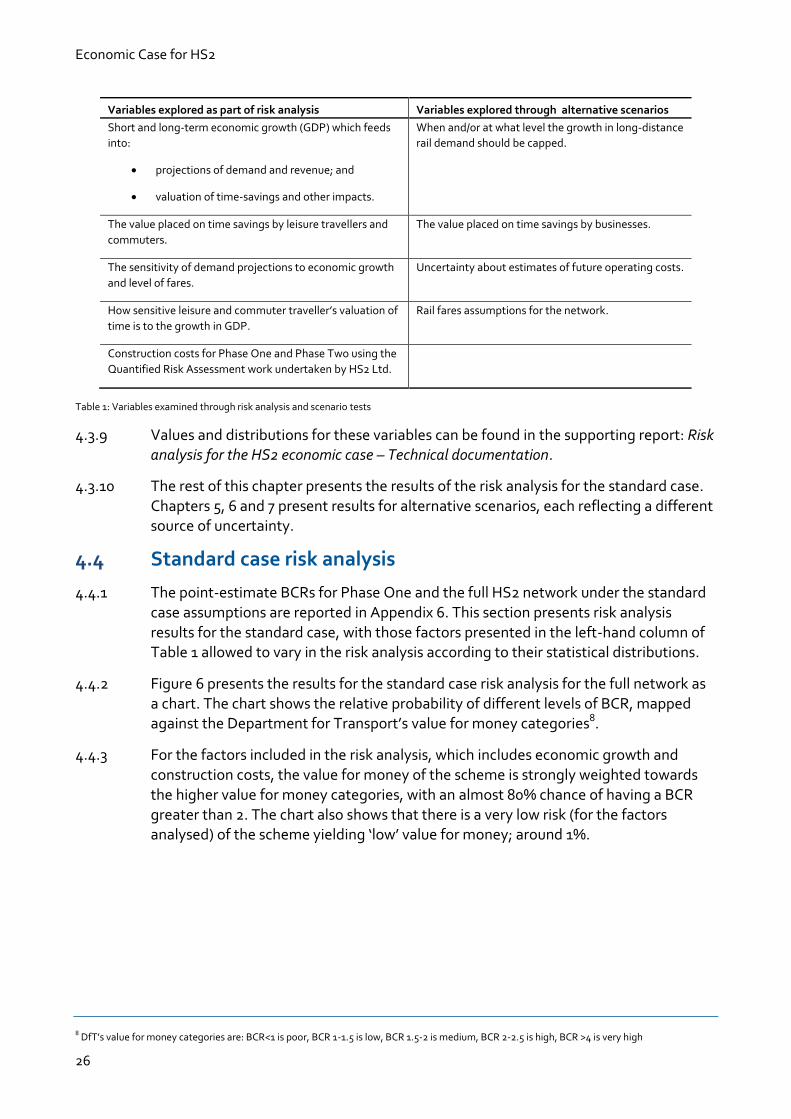
4.4.2 Figure 6 presents the results for the standard case risk analysis for the full network as a chart. The chart shows the relative probability of different levels of BCR, mapped against the Department for Transport’s value for money categories8.
4.4.3 For the factors included in the risk analysis, which includes economic growth and construction costs, the value for money of the scheme is strongly weighted towards the higher value for money categories, with an almost 80% chance of having a BCR greater than 2. The chart also shows that there is a very low risk (for the factors analysed) of the scheme yielding ‘low’ value for money; around 1%.
8 DfT’s value for money categories are: BCR<1 is poor, BCR 1-1.5 is low, BCR 1.5-2 is medium, BCR 2-2.5 is high, BCR >4 is very high
Economic Case for HS2
27
Figure 6: Results of analysis for full network BCR
4.4.4 One of the key determinants of the BCR is economic growth, which determines both how quickly demand grows in the model and how people value travel time savings (and other impacts) from the scheme. The risk analysis includes a wide range of potential rates of economic growth, including a significant proportion that are well below historic long run economic growth rates.
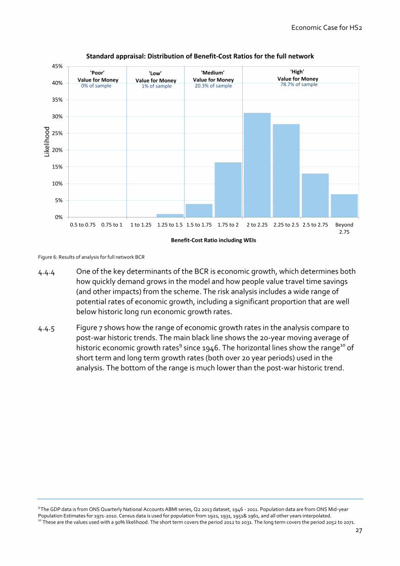
4.4.5 Figure 7 shows how the range of economic growth rates in the analysis compare to post-war historic trends. The main black line shows the 20-year moving average of historic economic growth rates9 since 1946. The horizontal lines show the range10 of short term and long term growth rates (both over 20 year periods) used in the analysis. The bottom of the range is much lower than the post-war historic trend.
9 The GDP data is from ONS Quarterly National Accounts ABMI series, Q2 2013 dataset, 1946 - 2011. Population data are from ONS Mid-year Population Estimates for 1971-2010. Census data is used for population from 1921, 1931, 1951& 1961, and all other years interpolated. 10 These are the values used with a 90% likelihood. The short term covers the period 2012 to 2031. The long term covers the period 2052 to 2071.
0%
5%
10%
15%
20%
25%
30%
35%
40%
45%
0.5 to 0.75 0.75 to 1 1 to 1.25 1.25 to 1.5 1.5 to 1.75 1.75 to 2 2 to 2.25 2.25 to 2.5 2.5 to 2.75 Beyond2.75
Like
liho
od
Benefit-Cost Ratio including WEIs
Standard appraisal: Distribution of Benefit-Cost Ratios for the full network
'Poor' Value for Money
'Low' Value for Money
'Medium' Value for Money
'High' Value for Money
0% of sample 1% of sample 20.3% of sample 78.7% of sample
Economic Case for HS2
28
Figure 7: Long run average GDP per capita growth rates: historic versus risk analysis assumptions
4.4.6 In the analysis, stronger rates of economic growth result in higher levels of value for money. However, results from our analysis show how the full network is resilient to even the lowest rates of economic growth. Even when the long-run growth rate of GDP is below 2%, the majority (90%) of the scenarios with that lower growth still result in medium or high value for money.
4.4.7 Figure 8 shows the same analysis for Phase One of the scheme. Compared with the
full network, variability in the distribution in the BCR is very similar, but on average the BCR for Phase One only of the scheme is lower.
1.0%
1.5%
2.0%
2.5%
3.0%
3.5%1
94
6-1
96
5
19
48
-19
67
19
50
-19
69
19
52
-19
71
19
54
-19
73
19
56
-19
75
19
58
-19
77
19
60
-19
79
19
62
-19
81
19
64
-19
83
19
66
-19
85
19
68
-19
87
19
70
-19
89
19
72
-19
91
19
74
-19
93
19
76
-19
95
19
78
-19
97
19
80
-19
99
19
82
-20
01
19
84
-20
03
19
86
-20
05
19
88
-20
07
19
90
-20
09
19
92
-20
11
20
ye
ar m
ovi
ng
ave
rage
GD
P g
row
th p
er
cap
ita
Moving average period
Compare Post war 20 year moving average GDP growth per capita with simulated GDP coverage
P5 Short term growth
P5 Long term growth
P95 Short term growth
P95 Long term growth
Actual moving average (20 years)

Economic Case for HS2
29
Figure 8: Results of analysis of Phase One only
4.4.8 The chart shows that, for the factors analysed, Phase One is much more likely (77%) to be medium or high value for money than low (23%), for the variables analysed.
4.5 Conclusions
4.5.1 The results in this chapter have shown that the standard economic appraisal for the scheme is resilient to varying a wide variety of important inputs to the case including: economic growth, the rate of growth in demand, construction costs and valuation in
leisure and commuting time. Different assumptions on these factors affect the value for money – both positively and negatively – but on the basis of this analysis the case is robust to wide ranges of different assumptions.
0%
5%
10%
15%
20%
25%
30%
35%
40%
45%
0.5 to 0.75 0.75 to 1 1 to 1.25 1.25 to 1.5 1.5 to 1.75 1.75 to 2 2 to 2.25 2.25 to 2.5 2.5 to 2.75 Beyond2.75
Like
liho
od
Benefit-Cost Ratio including WEIs
Standard appraisal: Distribution of Benefit-Cost Ratios for Phase 1
'Poor' Value for Money
'Low' Value for Money
'Medium' Value for Money
'High' Value for Money
0.5% of sample 23% of sample 65% of sample 11.6% of sample
Economic Case for HS2
30
5 Impact of long-term demand growth 5.1 Introduction
5.1.1 The rate of demand growth has a significant impact on the economic case for HS2, therefore a range of possible demand growth scenarios have been tested for this update to the Economic Case. The two factors that have been varied are a) the rate at which demand grows, and b) the level at which demand is capped.
5.1.2 Our general approach to forecasting demand growth remains as set out in the original February 2011 Economic Case. Guidance on the relationships between rail demand growth and other economic factors is set out in WebTAG and is, in large part, based on the rail industry’s Passenger Demand Forecasting Handbook (PDFH). In line with updates to WebTAG, our analysis now draws many of its parameters from the most recent version of the handbook - PDFH5.
5.2 Recent growth
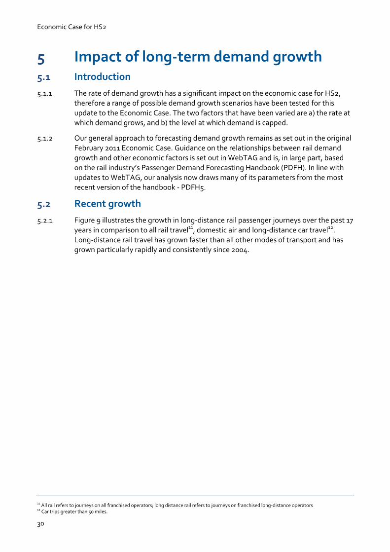
5.2.1 Figure 9 illustrates the growth in long-distance rail passenger journeys over the past 17 years in comparison to all rail travel11, domestic air and long-distance car travel12. Long-distance rail travel has grown faster than all other modes of transport and has grown particularly rapidly and consistently since 2004.
11 All rail refers to journeys on all franchised operators; long distance rail refers to journeys on franchised long-distance operators 12 Car trips greater than 50 miles.

Economic Case for HS2
31
Figure 9: Graph showing long-distance transport trends from 1995 to 201213
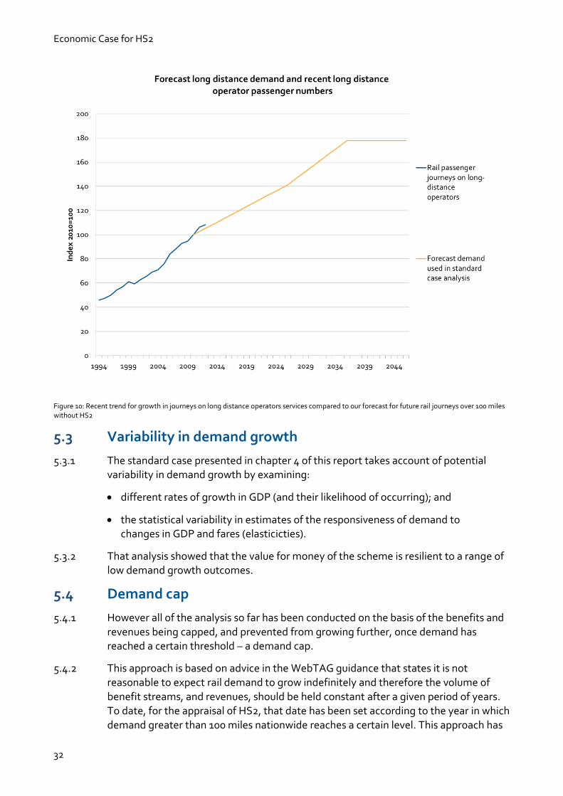
5.2.2 The very strong growth in demand for journeys on long-distance rail operators’ services since 1994 is shown in Figure 10. This has equated to an average year-on-year growth rate over the past 18 years of 4.9%. The graph also shows the assumed rate of growth of demand for the ‘Do Minimum’ in the economic case; at an average of 2.2% per annum from 2010 to 2036 this is lower than the recent trend.
5.2.3 This lower rate of growth is based on application of the PDFH5 forecasting parameters. Figure 10 also shows the level at which demand is capped in the standard case analysis.
13 Sources:
Office of Rail Regulation (ORR); Passenger journeys by sector; GB; financial year data. All rail – all franchised operators; Long distance rail – franchised long-distance operators Civil Aviation Authority (CAA); Domestic Terminal Pax Traffic; all reporting GB airports. Excludes: Alderney; Guernsey; Isle of Man; Jersey; Belfast City (George Best); Belfast International; City of Derry (Eglinton) National Travel survey; Average number of trips by trip length and main mode; trip length 50miles or more; GB; includes ‘Car/van driver’ and ‘Car/van passengers’. Number of trips calculated using GB population estimates from the Office for National Statistics (ONS).
75
100
125
150
175
200
225
250
1995
1996
1997
1998
1999
2000
2001
2002
2003
2004
2005
2006
2007
2008
2009
2010
2011
2012
Ind
ex (1
995=
100)
Journey Trends - Great Britain 1995-2012
Longdistance rail
All rail
Domestic air
Longdistance car
Economic Case for HS2
32
Figure 10: Recent trend for growth in journeys on long distance operators services compared to our forecast for future rail journeys over 100 miles without HS2
5.3 Variability in demand growth
5.3.1 The standard case presented in chapter 4 of this report takes account of potential variability in demand growth by examining:
different rates of growth in GDP (and their likelihood of occurring); and
the statistical variability in estimates of the responsiveness of demand to changes in GDP and fares (elasticicties).
5.3.2 That analysis showed that the value for money of the scheme is resilient to a range of low demand growth outcomes.
5.4 Demand cap
5.4.1 However all of the analysis so far has been conducted on the basis of the benefits and
revenues being capped, and prevented from growing further, once demand has reached a certain threshold – a demand cap.
5.4.2 This approach is based on advice in the WebTAG guidance that states it is not reasonable to expect rail demand to grow indefinitely and therefore the volume of benefit streams, and revenues, should be held constant after a given period of years. To date, for the appraisal of HS2, that date has been set according to the year in which demand greater than 100 miles nationwide reaches a certain level. This approach has

Economic Case for HS2
33
been agreed with DfT and is in accordance with the DfT’s guidance on appraising rail projects14.
5.4.3 In the modelling to support this update, this level of demand is reached in 2036, three years after the opening of Phase Two. This has changed from 2037 in the 2012 publications due to the same level of demand being forecast to be reached slightly earlier. The application of a demand cap means that the volumes of benefits and revenues15 are effectively held constant for the remaining 57 years of the appraisal period.
5.4.4 The next section of the document therefore looks at the impact of changing the demand cap to understand the risks and opportunities around the value for money of the scheme.
5.5 Demand cap with risk analysis
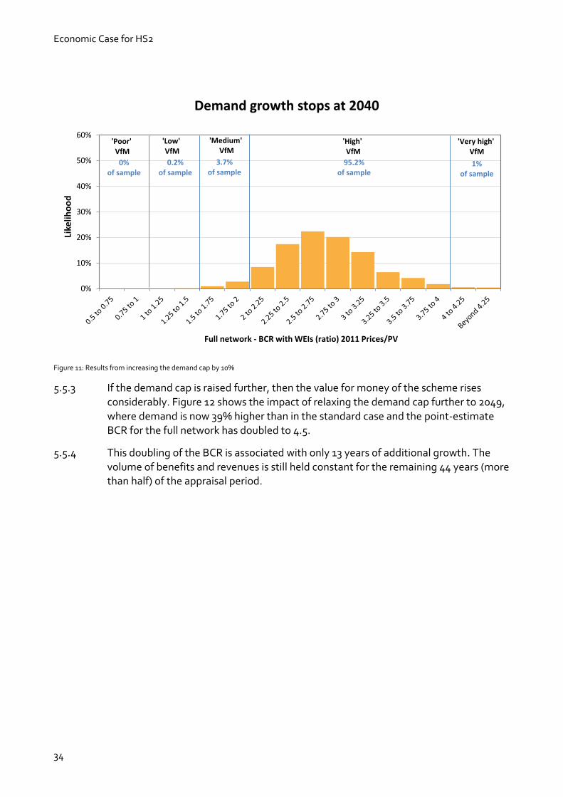
5.5.1 Figure 11 and Figure 12 show, for the full network, the impact of relaxing the demand cap on the potential value for money of the scheme. Figure 11 shows the impact of allowing demand to rise a further 10%, which would, on average, be only four more years of growth to 204016. The point-estimate BCR would be 2.8 and the likelihood of the scheme having a BCR greater than 2 rises to over 95% – compared to 75% for the standard case. More detailed results from this scenario are set out in Appendix 6.
5.5.2 It can be seen that even quite small increases in the demand cap can lead to significant increases in expected returns.
14 Guidance on Rail Appraisal – TAG Unit 3.13.1 – August 2012 http://www.dft.gov.uk/webtag/documents/archive/1208/unit3.13.1.pdf 15 When expressed in their natural units. 16 The average cap year is the arithmetic mean of the risk analysis results.
Economic Case for HS2
34
Figure 11: Results from increasing the demand cap by 10%
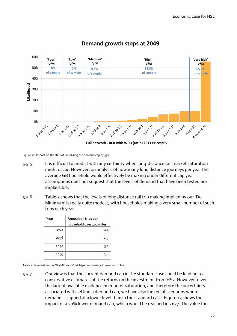
5.5.3 If the demand cap is raised further, then the value for money of the scheme rises considerably. Figure 12 shows the impact of relaxing the demand cap further to 2049, where demand is now 39% higher than in the standard case and the point-estimate BCR for the full network has doubled to 4.5.
5.5.4 This doubling of the BCR is associated with only 13 years of additional growth. The volume of benefits and revenues is still held constant for the remaining 44 years (more than half) of the appraisal period.
0%
10%
20%
30%
40%
50%
60%
Like
liho
od
Full network - BCR with WEIs (ratio) 2011 Prices/PV
Demand growth stops at 2040
'Poor' VfM
'Low' VfM
'Medium' VfM
'High' VfM
0%of sample
0.2%of sample
3.7%of sample
95.2%of sample
'Very high' VfM
1%of sample
Economic Case for HS2
35
Figure 12: Impact on the BCR of increasing the demand cap by 39%
5.5.5 It is difficult to predict with any certainty when long-distance rail market saturation might occur. However, an analysis of how many long distance journeys per year the average GB household would effectively be making under different cap year assumptions does not suggest that the levels of demand that have been tested are implausible.
5.5.6 Table 2 shows that the levels of long distance rail trip making implied by our ‘Do Minimum’ is really quite modest, with households making a very small number of such trips each year.
Year Annual rail trips per
household over 100 miles
2011 2.1
2036 2.9
2040 3.1
2049 3.6
Table 2: Forecast annual ‘Do Minimum’ rail trips per household over 100 miles
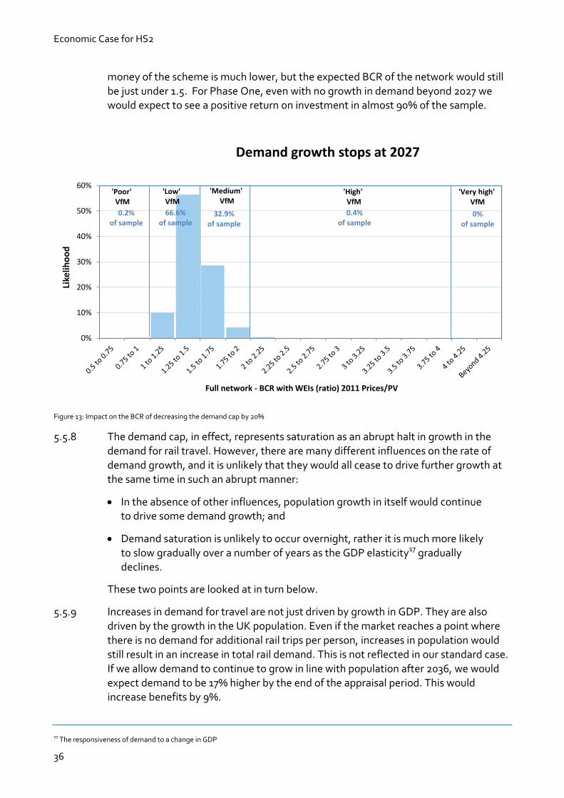
5.5.7 Our view is that the current demand cap in the standard case could be leading to conservative estimates of the returns on the investment from HS2. However, given the lack of available evidence on market saturation, and therefore the uncertainty associated with setting a demand cap, we have also looked at scenarios where demand is capped at a lower level than in the standard case. Figure 13 shows the impact of a 20% lower demand cap, which would be reached in 2027. The value for
0%
10%
20%
30%
40%
50%
60%
Like
liho
od
Full network - BCR with WEIs (ratio) 2011 Prices/PV
Demand growth stops at 2049
'Poor' VfM
'Low' VfM
'Medium' VfM
'High' VfM
0%of sample
0%of sample
0.4%of sample
33.8%of sample
'Very high' VfM
65.9%of sample
Economic Case for HS2
36
money of the scheme is much lower, but the expected BCR of the network would still
be just under 1.5. For Phase One, even with no growth in demand beyond 2027 we would expect to see a positive return on investment in almost 90% of the sample.
Figure 13: Impact on the BCR of decreasing the demand cap by 20%
5.5.8 The demand cap, in effect, represents saturation as an abrupt halt in growth in the
demand for rail travel. However, there are many different influences on the rate of demand growth, and it is unlikely that they would all cease to drive further growth at the same time in such an abrupt manner:
In the absence of other influences, population growth in itself would continue to drive some demand growth; and
Demand saturation is unlikely to occur overnight, rather it is much more likely to slow gradually over a number of years as the GDP elasticity17 gradually declines.
These two points are looked at in turn below.
5.5.9 Increases in demand for travel are not just driven by growth in GDP. They are also
driven by the growth in the UK population. Even if the market reaches a point where there is no demand for additional rail trips per person, increases in population would still result in an increase in total rail demand. This is not reflected in our standard case. If we allow demand to continue to grow in line with population after 2036, we would expect demand to be 17% higher by the end of the appraisal period. This would increase benefits by 9%.
17 The responsiveness of demand to a change in GDP
0%
10%
20%
30%
40%
50%
60%
Like
liho
od
Full network - BCR with WEIs (ratio) 2011 Prices/PV
Demand growth stops at 2027
'Poor' VfM
'Low' VfM
'Medium' VfM
'High' VfM
0.2%of sample
66.6%of sample
32.9%of sample
0.4%of sample
'Very high' VfM
0%of sample
Economic Case for HS2
37
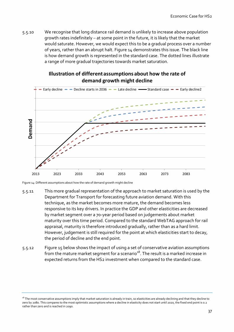
5.5.10 We recognise that long distance rail demand is unlikely to increase above population
growth rates indefinitely – at some point in the future, it is likely that the market would saturate. However, we would expect this to be a gradual process over a number of years, rather than an abrupt halt. Figure 14 demonstrates this issue. The black line is how demand growth is represented in the standard case. The dotted lines illustrate a range of more gradual trajectories towards market saturation.
Figure 14: Different assumptions about how the rate of demand growth might decline
5.5.11 This more gradual representation of the approach to market saturation is used by the Department for Transport for forecasting future aviation demand. With this technique, as the market becomes more mature, the demand becomes less responsive to its key drivers. In practice the GDP and other elasticities are decreased by market segment over a 70-year period based on judgements about market maturity over this time period. Compared to the standard WebTAG approach for rail appraisal, maturity is therefore introduced gradually, rather than as a hard limit. However, judgement is still required for the point at which elasticities start to decay, the period of decline and the end point.
5.5.12 Figure 15 below shows the impact of using a set of conservative aviation assumptions from the mature market segment for a scenario18. The result is a marked increase in expected returns from the HS2 investment when compared to the standard case.
18 The most conservative assumptions imply that market saturation is already in train, so elasticities are already declining and that they decline to zero by 2080. This compares to the most optimistic assumptions where a decline in elasticity does not start until 2020, the fixed end point is 0.2 rather than zero and is reached in 2090.
1
1.2
1.4
1.6
1.8
2
2.2
2.4
2013 2023 2033 2043 2053 2063 2073 2083
Dem
and
Illustration of different assumptions about how the rate of demand growth might decline
Early decline Decline starts in 2036 Late decline Standard case Early decline2

Economic Case for HS2
38
Figure 15: Results on the BCR of demand growth assumptions applied in the aviation industry
5.6 Impact of fares on demand and interaction with the demand cap
5.6.1 All of the analysis reported so far has been based the same fares assumption: fares
grow at RPI19+1% until 2036 (which is the demand cap year in the standard case), after 2036 fares grow in line with inflation. This assumption affects both the point at which our demand cap is reached because fares affect growth in demand and the level of revenue that the scheme will accrue. We have therefore tested some alternatives to understand the impact of this assumption.
5.6.2 Two alternative scenarios have been tested:
Fares grow at RPI+1% until 2020 and then at RPI till 2031; and
Fares grow at RPI+1% until 2020, then at RPI+2% until the demand cap is reached (2050).
5.6.3 Figure 16 shows the results from the, first, lower fares assumption. The results suggest that the value for money for HS2 falls with lower fares. The adoption of lower fares
results in the forecast demand rising to the level of the demand cap at a faster rate. In the scenario tested, the cap is reached in 2032. Once that level has been reached, the volume of demand is held constant, and the only impact of lower fares is lower revenue.
19 The Retail Price Index (RPI) provides a measure of the variation in the prices of retail goods and other items over time, and is used by the Department for Transport as a reference point for regulated fares policy
0%
10%
20%
30%
40%
50%
60%
Like
liho
od
Full network - BCR with WEIs (ratio) 2011 Prices/PV
Aviation demand assumptions
'Poor' VfM
'Low' VfM
'Medium' VfM
'High' VfM
0%of sample
0.6%of sample
3.9%of sample
56.6%of sample
'Very high' VfM
39%of sample

Economic Case for HS2
39
Figure 16: Results on the BCR of assuming lower future rail fares
5.6.4 The interaction of the demand cap with fare levels means that these results are difficult to interpret. Figure 17 illustrates this point by showing the range of BCR outcomes for the lower fares assumption but with a higher demand cap (+20%). Expected BCR of the scheme is now 2.5 to 3 compared to 1.5 to 2 in Figure 16 where low fares are assumed with a 2036 demand cap.
0%
5%
10%
15%
20%
25%
30%
35%
40%
45%
Like
liho
od
Full network - BCR with WEIs (ratio) 2011 Prices/PV
Low fares scenario
'Poor' VfM
'Low' VfM
'Medium' VfM
'High' VfM
0%of sample
2.8%of sample
61.5%of sample
35.8%of sample
'Very high' VfM
0%of sample

Economic Case for HS2
40
Figure 17: Benefit cost ratio results with low fare and high demand assumptions
5.6.5 For completeness, Figure 18 shows the impact of the higher fares assumption which pushes the demand cap out to 2049. This shifts the value for money of the scheme up, with a 30% likelihood of the BCR being greater than 4.
0%
5%
10%
15%
20%
25%
30%
35%
40%
45%
Like
liho
od
Full network - BCR with WEIs (ratio) 2011 Prices/PV
Low fares with 20% higher demand cap
'Poor' VfM
'Low' VfM
'Medium' VfM
'High' VfM
0%of sample
0.1%of sample
2.5%of sample
96.6%of sample
'Very high' VfM
0.9%of sample
Demand growth stops at 2038

Economic Case for HS2
41
Figure 18: Benefit cost ratio results with high fare and high demand assumptions
5.7 Differential fares and the impact of competition
5.7.1 The operational characteristics and regulatory environment in which HS2 might operate are, as would be expected at this stage in scheme development, undetermined. As part of a broader and longer term work programme, we have
started to investigate how different operating environments and responses by train operating companies might impact on the economic case.
5.7.2 There are a wide range of potential scenarios including changes to fares, service levels, train capacities or indeed combinations of all of these. Furthermore, Government has scope to influence the operating environment and the incentives which guide the commercial decisions of operators.
5.7.3 Our early work has considered how competition between conventional rail and HS2 operators on some routes might influence pricing decisions under the current fares regimes. In this scenario, our analysis indicates that conventional rail operators would have a commercial incentive to reduce fares to capture market share from HS2 on competed routes.
5.7.4 This is likely to limit the scope for HS2 to set higher fares across the board although the moderating effect of competition will be less for those passengers with the highest willingness to pay for the journey time improvements offered by HS2.
5.7.5 Therefore, depending on the regulatory regime there may be a mixed response with some fares higher than we have assumed in the standard case and some fares lower. Looking at fare differentials similar to those seen on other routes with fast/slow speed alternatives, such as London to Birmingham, our analysis suggests that whilst
0%
5%
10%
15%
20%
25%
30%
35%
40%
45%
Like
liho
od
Full network - BCR with WEIs (ratio) 2011 Prices/PV
High fares scenario
'Poor' VfM
'Low' VfM
'Medium' VfM
'High' VfM
0.1%of sample
1.1%of sample
2%of sample
66%of sample
'Very high' VfM
30.9%of sample

Economic Case for HS2
42
reductions in fares on conventional rail will reduce revenue on HS2, this will be broadly
off-set by an increase in revenue on conventional rail. The value for money of the scheme (which takes into account both effects as well as the benefit passengers get from lower fares) is therefore not significantly impacted by such behaviour.
5.7.6 Our work so far, has therefore not suggested any major impacts for value for money. However, this strand of our work is in its very early stages and subject to significant further modelling and scenario development.
5.8 Conclusions
5.8.1 The demand cap within the standard case exerts a strong influence on the appraisal of the value for money of the HS2 scheme. Whilst there is a lack of evidence to underpin any specific assumption on when the demand for long distance rail might saturate, it can be seen that standard assumptions could well be conservative and the upside risks to value for money are much greater than the downside risks to the scheme.
5.8.2 For the longer-term demand growth scenarios tested the point-estimate BCR lies between 2.8 and 4.5.

Economic Case for HS2
43
6 Monetary valuation of time savings 6.1 The value of time in appraisal
6.1.1 All of the analysis set out in chapter 4 is based on the techniques set out in the Department for Transport’s WebTAG transport appraisal guidance. The standard approach to transport cost benefit analysis, as specified in WebTAG, requires a monetary valuation to be placed on the impacts that an investment will have on the travelling experience of transport users.
6.1.2 Most of these impacts are first expressed in units of time e.g. time spent travelling or time spent in crowded conditions, and are then converted in the analysis into units of money so that the benefits can be compared to the costs of the investment. This conversion is achieved with a set of ‘values of time’ that correspond to different aspects of journey time.
6.1.3 Over the years there have been numerous studies into values of time, which have used a variety of different techniques to try to determine how much transport users are
willing to pay to reduce different aspects of their travel time. The studies have also shown that the values are influenced by a wide range of factors, including the purpose and the length of the journey.
6.1.4 A user’s journey purpose has a particularly strong influence on the values of time, with studies showing that people travelling in the course of their work are generally willing to pay considerably more to save elements of their travel time, than people travelling for their own ends. This distinction is particularly important for the cost benefit analysis of HS2 as our network is designed to provide for rapid journeys between city
centres, and is therefore likely to carry a relatively high proportion of business travellers.
6.1.5 Despite the apparent simplicity of the ‘value of time’ concept, the studies have
revealed that there is no single, simple way of measuring the values that can be relied on in all circumstances.
6.1.6 Over the course of the last year the DfT has reviewed its approach to valuing business travel time savings. Its conclusions are set out in the document Understanding and Valuing the Impacts of Transport Investment and summarised in the box below. As a result, the values of time presented in the WebTAG guidance are being updated. Table 3 below shows the new values of time for business travellers (rail) and non-business travellers.
Travel Purpose Old Values of Time New Values of Time
Business £47.18 £31.96
Commuting £6.46 £6.81
Leisure £5.71 £6.04
Table 3: Changes in value of time used in WebTAG (2010 prices)

Economic Case for HS2
44
6.1.7 These new values, published alongside this document, will shortly be mandated for
use on all transport schemes, and it is on this basis that we have used them for the majority of the analysis presented in this report. A scenario using the old WebTAG 2012 values of time is set out in Appendix 6.
DfT review of values of time for business travellers
Values of travel time savings should represent what people and businesses would be willing
to pay for quicker journeys. Over the last year, the Department has undertaken a
comprehensive review of different approaches for deriving this willingness-to-pay for
business travellers. This has included updating the values in WebTAG with the most recent
available data and comparing those updated values with the existing evidence base of
values from alternative approaches.
The comparison of values resulting from different approaches is shown in the chart below.
While the assumptions and methods vary between approaches, they are all aiming to
estimate the same thing: what businesses would be willing to pay for travel time savings.
Sources: Valuation of travel time savings for business travellers, ITS Leeds, 2013; and DfT analysis
The solid line error bars represent robustly calculated confidence intervals. The dotted lines are indicative representations of potential variability as the sample sizes are not sufficient to support calculation of formal confidence intervals.
The wide range in the values presented in the chart, both within and between approaches,
demonstrates the variability and uncertainty around what businesses would be willing to pay
for travel time savings. However, the updated values given in WebTAG of around £32/hour
for rail travel and £27/hour for car travel are firmly towards the centre of this range and,
therefore, the Department has concluded that these values are a suitable representation of
businesses’ willingness-to-pay.
Economic Case for HS2
45
6.2 Value of time scenario tests
6.2.1 The results of research carried out by the Institute of Transport Studies commissioned by the DfT to support the review raise questions about the suitability of using an ‘average’ value of time in appraising high-speed rail schemes. In their report the authors conclude that the evidence across a range of studies supports a higher business valuation in the context of high speed rail, the report states: ‘across the central values for each study, the value of time was on average around 50% larger than the gross wage rate, and across the six UK studies it was 40% larger’.
6.2.2 The higher observed values may be the result of a number of factors, including:
the long-distances served by high-speed rail services (length of journey is known to exert a strong influence over the value of time);
the higher productivity of business travellers that make use of the services;
the larger time savings offered by high speed rail schemes (there may be a non-linearity in the value placed on different sizes of time savings); and
other effects not captured by the cost-savings approach , such as the ability to avoid overnight stays, and the additional productivity achieved by being able to spend more time with the client.
6.2.3 On the balance of the evidence presented in the ITS Leeds study, we think that there is good cause to believe that high speed rail schemes should be assessed with values of time that are higher than the standard WebTAG values. However, in the interest of balance, we have tested scenarios where the values of time are both higher and lower than the standard values. The results of these tests are set out below.
6.3 Results from value of time scenarios
6.3.1 This section presents the outcome of three scenarios:
the standard case;
an alternative value of time scenario using HSR evidence; and
a 'low value of time' scenario.
All these scenarios assume a 2036 demand cap.

Economic Case for HS2
46
6.3.2 The values for the scenarios are set out below.
Travel Purpose Standard case Low value of
time
Alternative value
of time
Business average
Long distance
Regional
£31.96
£26.10
£44.66
£31.96
Commuting average
long distance
regional
£6.81 £6.81
£12.31
£6.91
Leisure average
Long distance
Regional
£6.04 £6.04
£10.72
£5.28
Table 4: Values of time used in scenarios (2010 prices)
6.3.3 The standard case uses the general purpose values of time as set out in the draft WebTAG guidance of October 2013.
6.3.4 To create the ‘alternative value of time’ scenario, we have increased the WebTAG 2013 standard business value of time for long distance rail users by 40% in line with the ITS Leeds research20. We have also varied non-work values according to time savings by trip length (as the standard value is averaged across trip length)21.
6.3.5 For the ‘low value of time’ scenario, we sought advice from the Department for
Transport on an appropriate lower bound value for business time savings. The Department recognised the relatively small range of existing studies which derive values of time for high speed rail journeys and so proposed a 'lower bound' value
based on the larger number of studies which derive values of time on all inter-urban rail journeys. The research commissioned by the DfT suggested this would imply a lower bound which applies a 20% reduction to the existing WebTAG 2013 values. This effectively assumes that high speed rail passengers have similar values of time to other rail passengers, a conclusion that is at odds with the existing evidence as noted above.
6.3.6 The ‘low value of time’ scenario does not explicitly model a lower value of time for non-work trips because the variation around these values is already included in the risk analysis22.
6.3.7 Figure 19 and Figure 20 show how the likelihood of the BCR being above two changes for different values of time for the whole network. Two conclusions can be drawn from the charts.
20 Note this is actually lower than the 25% increase on the WebTAG 2012 values proposed by the study. 21 As we have changed the non-work time values we cannot vary them in the risk analysis, so for this scenario there is no variability in these inputs. 22 The WebTAG guidance recommendation of a test of-25% reduction in non-work benefits is in fact based on the same evidence as we use to put likelihoods around these values in the risk analysis.
Economic Case for HS2
47
6.3.8 First, the business case for HS2 is robust to a wide range of values of time. There are positive returns to investment, even with:
lower values of time, which are not actually compatible with the ITS Leeds evidence on high speed rail values;
the upper end of the range of our cost estimates;
long-term economic growth forecasts that are lower than those experienced in any 20 year period since the Second World War; and
the most pessimistic view on other factors in the risk analysis.
6.3.9 We have also tested the impact of the ‘low value of time’ scenario for Phase One separately, and this conclusion holds. Results show that a positive return on investment is expected in 98% of scenarios.
6.3.10 The adoption of values that reflect the evidence from high speed rail studies and on long-distance trip making would result in significantly higher benefit cost ratios. In these circumstances the expected benefit cost ratio for the whole full network would be over 3. These are in marked contrast to those in the standard case. Appendix 6 sets out the point estimate BCR from this alternative value of time scenario.

Economic Case for HS2
48
Figure 19: Benefit cost ratio results with alternative value of time assumptions
Figure 20: Benefit cost ratio results with low value of time assumptions
0%
5%
10%
15%
20%
25%
30%
35%
40%
Like
liho
od
Full network - BCR with WEIs (ratio) 2011 Prices/PV
Higher willingness to pay for long journeys
'Poor' VfM
'Low' VfM
'Medium' VfM
'High' Value for Money
0%of sample
0%of sample
0.6%of sample
95.1%of sample
'Very high' VfM
4.3%of sample
0%
5%
10%
15%
20%
25%
30%
35%
40%
Like
liho
od
Full network - BCR with WEIs (ratio) 2011 Prices/PV
Low Value of Time Scenario
'Poor' VfM
'Low' VfM
'Medium' VfM
'High' Value for Money
0%of sample
3.3%of sample
50.4%of sample
46.4%of sample
'Very high' VfM
0%of sample

Economic Case for HS2
49
7 Construction and operating costs 7.1 Introduction
7.1.1 Chapter 4 looked at the standard case with risk analysis. Chapters 5 and 6 have looked at the case using different assumptions on the demand cap and value of time. This chapter examines the impact of cost assumptions.
7.2 Construction costs
7.2.1 This section of the document sets out the different estimates of construction costs, how they should be interpreted in the context of the economic case and their impact on the value for money of the scheme.
Key terminology Definition/explanation Phase One costs used in
the economic case*
(2011 prices)
Phase Two costs used in
the economic case* (2011
prices)
Base cost The base cost estimated for the scheme
using best estimates for all elements of
construction
£15.5 billion
£12.5 billion
Quantified Risk
Assessment
(QRA)
Quantitative assessment of the risks and
opportunities to the base cost. A
likelihood is attached to different
outcomes giving a probability distribution
for different levels of cost which can be
used in risk analysis. See Appendix 3 for
more detail.
Full QRA for Phase One
exists which has replaced
Optimism Bias.
QRA for Phase Two is less
well developed, reflecting
the stage of development.
Phase Two therefore
includes some elements of
QRA and some Optimism
Bias.
Target price The budget which HS2 Ltd has been set
for Phase One. There are a set of
mechanisms and allocation of risks to
support delivery of this target.
£17.1 billion N/A due to stage of phase
development
P50 cost In line with Green Book guidance this is
the level of risk/contingency assumed for
the ‘standard’ appraisal case.
£19.2 billion £19.0 billion
P95 cost Taking account of the risks and their
probabilities, this is the highest amount
of contingency likely to be required. In
QRA terms, costs are 95% likely to be
within this envelope.
£21.2 billion £21.2 billion
* These costs are slightly lower than those reported in the spending review as they do not include the spending in 2012/13. As this spending has already occurred these are sunk costs, and are therefore not included in economic appraisal, in line with WebTAG 3.5.9.
Table 5: Varying construction costs for each Phase dependant on the amount of risk included
7.2.2 The Quantified Risk Assessment (QRA) information we have for construction costs enables this to form part of the standard case risk analysis. The impact of different construction costs outcomes using the range of costs in Table 5 is therefore included in the distribution of BCRs in Figure 6 and Figure 8 in chapter 4. However, we have also drawn out some analysis to show explicitly how the scheme’s value for money changes with specific assumptions on costs.
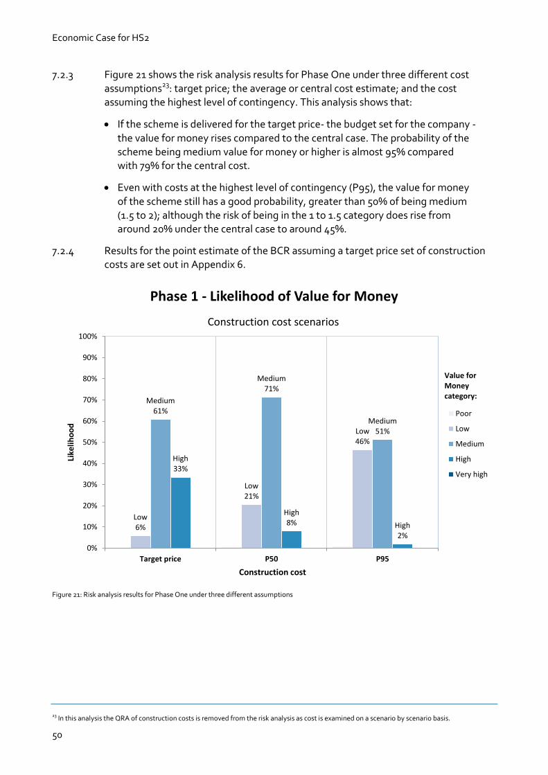
Economic Case for HS2
50
7.2.3 Figure 21 shows the risk analysis results for Phase One under three different cost
assumptions23: target price; the average or central cost estimate; and the cost assuming the highest level of contingency. This analysis shows that:
If the scheme is delivered for the target price- the budget set for the company -
the value for money rises compared to the central case. The probability of the scheme being medium value for money or higher is almost 95% compared with 79% for the central cost.
Even with costs at the highest level of contingency (P95), the value for money
of the scheme still has a good probability, greater than 50% of being medium (1.5 to 2); although the risk of being in the 1 to 1.5 category does rise from around 20% under the central case to around 45%.
7.2.4 Results for the point estimate of the BCR assuming a target price set of construction costs are set out in Appendix 6.
Figure 21: Risk analysis results for Phase One under three different assumptions
23 In this analysis the QRA of construction costs is removed from the risk analysis as cost is examined on a scenario by scenario basis.
Low6%
Low21%
Low46%
Medium61%
Medium71%
Medium51%
High33%
High8% High
2%
0%
10%
20%
30%
40%
50%
60%
70%
80%
90%
100%
Target price P50 P95
Like
liho
od
Construction cost
Phase 1 - Likelihood of Value for Money
Poor
Low
Medium
High
Very high
Value for Moneycategory:
Construction cost scenarios

Economic Case for HS2
51
7.2.5 Figure 22 shows some similar results for the full network. The analysis shows that:
For the P50 estimate of construction costs for the whole network, the
expected value for money of the scheme is high, with an 80% probability of being 2 or higher; and
Even with the highest level of contingency, the expected value for money of the scheme is 'high', although the probability falls to just over 50%.
Figure 22: Risk analysis results for the full network under two different assumptions
7.2.6 It is clear that the out-turn cost of the scheme will impact on the value for money, which is why maintaining a vigorous and disciplined approach to cost control is a key priority for HS2 Ltd. However, our analysis shows that:
with central case estimates of contingency the overall network is very firmly in the high value for money category; and
whilst the value for money is reduced by high levels of contingency being
called upon, on the basis of this analysis, this is highly unlikely to ultimately result in an out-turn BCR of less that 1.
Low1%
Low2%
Medium19%
Medium45%
High81%
High53%
0%
10%
20%
30%
40%
50%
60%
70%
80%
90%
100%
P50 P95
Like
liho
od
Construction cost
Full network - Likelihood of Value for Money
Poor
Low
Medium
High
Very high
Value for Moneycategory:
Construction Cost Scenarios

Economic Case for HS2
52
7.3 Operating costs
7.3.1 Since the August 2012 update to the economic case, the operating cost assumptions for both HS2 and the savings from the classic network have undergone a major review24. Two of the major changes that came out of that review were:
The removal of optimism bias on classic line savings as a more prudent approach to estimating savings; and
Improvements to cost estimates for the HS2 scheme and a reduction in the
level of optimism bias on some items of HS2 costs reflecting the development of the scheme.
7.3.2 The level of optimism bias (OB) applied to HS2 service operating costs now ranges from 10% to 41% depending on the item. The average level of OB in the standard case
is 21%. To test the sensitivity of the value for money, we have conducted two scenarios:
An optimistic assessment of operating costs, with optimism bias on all HS2 costs set at 10%; and
A pessimistic assessment of operating costs, with optimism bias on all HS2 costs set at 41%.
7.3.3 Figure 23 shows the results of this analysis for the full network. It is clear that the value for money of the scheme is sensitive to assumptions on operating costs, but we have no reason to believe that the downside risks outweigh the upside risks.
24 More detail on the outcomes of the review is set out in the Cost and risk status report.

Economic Case for HS2
53
Figure 23: Results for the full network of varying the level of optimism bias for the operating costs
Low0%
Low1%
Low4%
Medium8%
Medium20%
Medium58%
High92%
High79%
High38%
0%
10%
20%
30%
40%
50%
60%
70%
80%
90%
100%
10% OB 22% 41% OB
Like
liho
od
Optimism Bias on Operating Cost
Full network - Likelihood of Value for Money
Poor
Low
Medium
High
Very high
Value for Moneycategory:
Operating Cost Scenarios
Economic Case for HS2
54
8 Beyond conventional appraisal 8.1 Limitations of our economic appraisal
8.1.1 Most of the results that are presented in this document are based on the analytical techniques set out in the DfT's WebTAG guidance. Whilst we have used some significant extensions to the approach to test the resilience of the results from the cost benefit analysis, the core techniques are essentially the same as would be employed for any other transport scheme.
8.1.2 The WebTAG approach has been developed and refined over several years to provide a common basis for the comparison of proposals. In order to provide that common basis, some simplifying assumptions and approximations have been used within the guidance to ensure that the amount of effort required to complete an assessment is proportionate to the impact of the decision at hand.
8.1.3 HS2 is an unusual proposal in many respects. It is both national in scale, and yet it strongly impacts on existing transport networks at a local level. It offers large step-
changes in journey time and accessibility far larger than the majority of transport schemes and it is likely to have significant impacts on behaviour, with implications for future land-use patterns, particularly around its stations. The large changes in journey time and accessibility create new opportunities for significant changes to the geographic distribution of economic activity across the country.
8.1.4 Economic activity is unevenly distributed in Britain. Like any other country our cities make a disproportionate contribution to economic output, and there is significant variation in productivity, which in London and the South East is considerably higher
than anywhere else. There are a number of reasons why activity and prosperity is not evenly distributed – some rooted in history, and competing forces of agglomeration (which tends to concentrate activity in dense, productive locations), and the cost of
delivering a good or service (which tends to disperse activity so that it is produced closer to where it is consumed). HS2 could affect the balance of these forces and alter the geographical distribution of economic activity across Britain.
8.1.5 Our standard economic appraisal adopts simplifying assumptions, such as fixed land use, which means it is unlikely to capture these impacts on economic geography. In addition to this, because the approach takes a national perspective in the presentation of net benefits, it is limited in its ability to explain the more local or regional implications of the scheme.
The impact of HS2 on economic geography
8.1.6 To address this issue we commissioned a separate programme of work to try to identify the full scope for HS2 to impact on the economy, including the potential impact on the distribution of economic activity. This programme of work has been reviewed by an advisory panel of independent experts set up by HS2 Ltd to provide advice on the scope, design and delivery of an analytical work programme25.
25 For full details of the advisory panel, see: http://www.hs2.org.uk/about-hs2-ltd/external-challenge-groups

Economic Case for HS2
55
8.1.7 A key focus has been on the benefits that would result from HS2 providing better
connections between city centres. The effect of connecting places in this way could be substantial in the context of HS2, since improvements in connections between places facilitate increased trade and specialisation.
8.1.8 Better connections create opportunities for a reorganisation of economic activity between places, with firms, plants and offices moving to new – and now more efficient – locations. The changes arise because better connections improve access to markets, suppliers, competitors, and labour. For example, firms in London can access the Manchester market more easily (and vice versa) and firms in Manchester have better access to specialist intermediate suppliers and business services located in London (and vice versa).
8.1.9 With HS2, cities effectively become 'closer' to each other, which makes it easier for
businesses (and people) to interact and coordinate activities across city boundaries. This opens up opportunities for closer integration, and trade, with the potential for each city to develop its own specialism. Greater trade and specialisation could offer the potential for additional benefits, beyond those captured within our economic appraisal, through increased productivity. A paper written for HS2 Ltd on the economic impacts of HS2, by Bridget Rosewell (Volterra Partners) and Tony Venables (University of Oxford) provides a theoretical framework to explain the mechanisms by which connecting places may lead to additional productivity gains26.
8.1.10 Alongside the consideration of theoretical frameworks, KPMG has been working on behalf of HS2 Ltd to develop a methodological framework to analyse the potential scale, range and distribution of regional economic impacts associated with the investment in HS227.
8.1.11 The KPMG approach considers how patterns of economic activity vary across markets and geographies and how these differences relate to differences in levels of transport connectivity between businesses and labour markets. The analysis then measures the impact of HS2 on business and labour connectivity and examines how the measured improvements in connectivity affect economic output, drawing on empirical analysis of current travel patterns and observed relationships between connectivity and economic growth.
8.1.12 Although the analysis draws on some of the same inputs as our economic appraisal, it does not seek to value travel time and cost changes directly. Instead, it aims to understand how these changes to travel times and costs influence regional economic performance, both in terms of overall economic productivity and the location of economic activity. The analysis provides an alternative approach to conventional
transport appraisal and the estimated net benefits should not therefore be necessarily considered as additional to those estimated in the economic case.
8.1.13 The results should be considered as a first step in assessing the scheme’s potential impact on the economy, particularly as it is based on data and assumptions used to
26 High Speed Rail, Transport Investment and Economic Impacts - http://www.hs2.org.uk/news-resources/publications/economic-documents 27 HS2: The Regional Economic Impact (KPMG) - http://www.kpmg.com/uk/en/issuesandinsights/articlespublications/pages/hs2-regional-economic-impact.aspx

Economic Case for HS2
56
support the August 2012 iteration of the economic case. It is anticipated that forecast
impacts will be updated as the broader programme of work develops, particularly to take account of the assumptions underlying the current version of the standard economic analysis.
8.1.14 Nevertheless, the work provides valuable new evidence on the potential distribution of the benefits of HS2 across Great Britain, and the possible boost to regional economies.
8.1.15 The analysis shows that the whole country could benefit from an increase in annual productivity of £15 billion by the time HS2 reaches Manchester and Leeds28. The estimated productivity impacts extend widely beyond areas on the immediate HS2 network, with significant impacts for areas benefiting from released capacity or reduced journey times from high speed services which run on to the classic network.
8.1.16 The analysis shows that London does well as a result of HS2, with up to £2.8 billion of the total annual productivity gains, but the remaining £12 billion is spread across the country, with particularly strong gains in the Midlands and the North. Between £6.4bn
and £8.6bn is estimated to be generated in HS2 city regions outside London, and between £5bn and £7bn generated in the rest of Great Britain (largely brought about by the use of freed-up capacity which results on widespread improvements to rail services on the classic network, particularly on long-distance routes).
8.1.17 Figure 24 sets out the results geographically focusing on the HS2 network. Areas not directly on the HS2 network could also experience significant benefits from the scheme.
28 Results are modelled for 2037, and presented in 2013 prices.

Economic Case for HS2
57
Figure 24: Changes in economic output (£, 2013 prices) after investment in HS2 – conurbations on the HS2 network
Economic Case for HS2
58
To further understand the sensitivity of these results to some of the key inputs to the 8.1.18analysis, the report also presents the findings of sensitivity testing.
The first of these tests considers an alternative approach to deriving the relative 8.1.19importance of individual connectivity measures for rail and road with respect to both labour connectivity and business-to-business connectivity. By using a ‘mode-share’ approach the potential annual productivity gain reduces by 50%, to £8bn.
The second test uses an illustrative 50% reduction to business users’ value of in-8.1.20vehicle time on total productivity impacts. Results show that this 50% reduction in value of time reduces the potential annual productivity gain by 20%, to £12bn.
These tests have been included in an attempt to quantify areas where there is 8.1.21
potential for downside risk. However, the report also identifies a number of areas where there is potential upside risk, but where further work is required before we can attempt to quantify through sensitivity testing. For example, this analysis excludes the potential benefits from international connectivity and competitiveness, intra-zonal trips, freight, and relief of growth constraints not accounted for in economic forecasts.
This is early work and it is difficult to draw direct comparisons with the standard 8.1.22methodology. However, we believe it suggests there may be additional benefits above those considered in the standard case. The next section sets out a comparison between the DfT Transport appraisal framework which is used for the standard case and the KPMG Regional Impact Analysis Methodology.
Comparing the DfT Transport Appraisal Framework and KPMG Regional Impact Analysis Methodology
8.1.23 In theory, both approaches are attempting to measure the same thing - the economic benefits from increased economic output generated as a result of investment in transport – and should deliver the same result. However, in practice, results differ because of differences in analytical frameworks, data quality/availability, and measurement.
8.1.24 Although the KPMG analysis shares many of the same base data inputs with the HS2 economic appraisal, the specific results are not directly comparable (and certainly not additive) given a number of important fundamental differences, as set out in Table 6 below.
KPMG HS2 Economic Appraisal
RESULTS/Differences £15bn annual productivity gain
(modelled for 2037, in 2013 prices)
£71bn net benefits
Benefit Cost Ratio = 2.3 (including wider impacts)
(in 2011 prices and present value)
Productivity gain (business user benefits and
wider impacts) = £53.8 billion.
What is the question we
are trying to answer?
What is the potential impact on
productivity and business location?
Does the proposed scheme represent value for
money?

Economic Case for HS2
59
Metrics Productivity, gross value added (GVA) Economic welfare
Basic methodological
approach
To forecast the impact of improvements in
connectivity on productivity and business
location.
To forecast all welfare impacts (to economy,
environment and people). These include
- Transport user benefits
- Wider economic impacts associated with
agglomeration, imperfect competition, and
increased labour force participation.
- Other impacts (noise, carbon, safety)
- Tax impacts (loss of indirect tax as a result of fewer
car passengers)
Behavioural response Assumes land use is not fixed: businesses
are able to respond to the scheme by
changing location.
Assumes land use is fixed: does not model impacts
of any potential change in the location of economic
activity. Potential for economic case to be further
developed to include changes in land use.
Time horizon Modelled for single future year (2037).
Impact expected to persist, but no profiling
modelled.
Costs and benefits estimated and profiled during
construction and 60 year period from completion of
Phase Two.
Distribution/location
effects
Analysis models productivity impacts for
235 ‘zones’ across GB – under a low and
high scenario for location effects. This
allows a disaggregation of productivity
impact by region/city region/zone.
Appraisal looks only at the net national impact. It
does not provide a distribution of impacts at sub-
national level.
Attribution Recognises the role transport can play as
an enabler of growth, analysis looks at the
potential effects assuming no supply side
constraints. Given that estimates reflect
potential opportunity, it is not possible to
apportion direct impact of the scheme.
Appraisal designed to isolate economic impacts that
can be directly attributed to the scheme.
Methodology has limited coverage of the
transmission mechanisms between changes to
transport outputs e.g. journey time and economic
outcomes.
Maturity and wider
consensus on
methodological
approach
It is acknowledged that this is a highly
complex area, where methodology
continues to develop. There are a number
of approaches available, each with their
own strengths and weaknesses, and no
consensus on a preferred approach.
This analysis builds on previous
connectivity models developed by KPMG,
with the key extension to include location
effects.
The Economic Case is carried out in line with
Department for Transport and HM Treasury
appraisal frameworks. Although there is some
debate about specific assumptions/implementation,
the underlying framework is well-established and
has been developed over many years, and is
considered best practice internationally in the
transport industry.
Table 6: How the KPMG report and the HS2 economic case vary in their analysis of the economic impact of HS2 network
8.1.25 The new analysis from KPMG should be seen as a complement, and not a substitute, to the economic appraisal. There are a number of important caveats to the KPMG results, mainly:
There are difficulties in estimating the elasticities for individual connectivity
measures. The analysis includes a sensitivity test to capture this uncertainty, but it cannot be overcome with statistical analysis. Further work is required to refine the approach.
Economic Case for HS2
60
The analysis necessarily assumes direct causality between connectivity and
productivity, but it has not been possible to provide evidence for this causality.
The analysis does not consider potential supply-side constraints, such as the availability of land, and as such only demonstrates the opportunity for productivity gains.
Impacts are dependent on other investments and decisions following the transport investment.
Due to the timing of the analysis, its results are based on data from the August 2012 transport model, and will need to be revised to reflect the October 2013 update.
There are also a number of ‘known un-knowns’ which could present upside
risk, although further evidence is required about these: the KPMG analysis models a closed economy (no inward investment, migration, or benefits from improved international connectivity); no account is taken of the potential for HS2 to relieve capacity constraints (future growth forecasts taken as given); analysis is zero-sum (no dynamic feedback effects for productivity gains to lead to job creation or re-investment); and it does not capture potential benefits from freight or short distance (intra-zonal) trips.
8.1.26 This work is presented as provisional and will continue to be developed in consultation with the wider academic community. Nevertheless, it provides a valuable addition to the evidence base.
8.2 The limits to the standard approach for calculating benefits
8.2.1 In addition to the impact on economic geography, during our analysis to update this economic case we have increased our understanding of how the very large reductions in journey time brought about by HS2 are affecting the appraisal calculus. Specifically, how these large reductions may be stretching the limits of some of the appraisal calculus that is used to estimate the transport user benefits. Whilst we expect that these issues are by no means unique to the appraisal of HS2 - they are likely to be an issue for other transport interventions as well - the significant changes brought about by the HS2 scheme mean that they are more evident.
8.2.2 One of the fundamental elements of the standard WebTAG approach is the calculation of changes in measures of 'consumer surplus' for transport users. 'Consumer surplus' is, in essence, a measure of the amount of enjoyment that is taken from consuming a good, over and above the amount that someone paid for it. In
transport terms this is the sum total of the difference between how much a transport user is willing to pay for an option (measured in terms of money and journey time) and the amount that the user would actually have to pay.
8.2.3 In WebTAG transport appraisal, the change in this total is calculated with a mathematical relationship that is commonly referred to as the 'rule of a half'. The full rationales for the use of the 'consumer surplus' and 'rule of a half' approaches are set out in unit 3.5.3 of the WebTAG guidance.

Economic Case for HS2
61
8.2.4 The 'rule of a half' is an approximation, which is expected, under certain conditions, to
result in the mis-estimation of benefits. These circumstances include (a) large changes in demand or journey times, and (b) change in land-use patterns in response to a scheme.
8.3 The impact of non-linearities in demand relationships
8.3.1 Under the first of these conditions mis-estimation of benefits can result from the reliance of the 'rule of a half ' on an approximation when calculating consumer surplus. In essence the 'rule of a half' approach relies upon a linear approximation of the relationships between journey times and the levels of demand for the different options facing transport users. In circumstances where changes in demand or journey times are very small, the assumption that the relationship is linear has minimal impact on results. If changes in journey times or demand are larger, then any non-linearity in
the relationships can lead to mis-estimation of the size of the change in consumer surplus.
8.3.2 Figure 25 illustrates the effect. The rule of a half calculations are attempting to
measure the solid blue area between points ABT1T0. However the non-linearity of the demand curve leads - in this instance - to an overestimation of the change in consumer surplus equivalent to the hatched area on the chart.
Figure 25: The potential for mis-estimation of benefits from the rule of a half
8.3.3 The sign and size of the mis-estimation depends on a number of different factors including the mathematical formulation of the relationship between demand and journey time, and the size of the changes in journey times themselves. Our demand
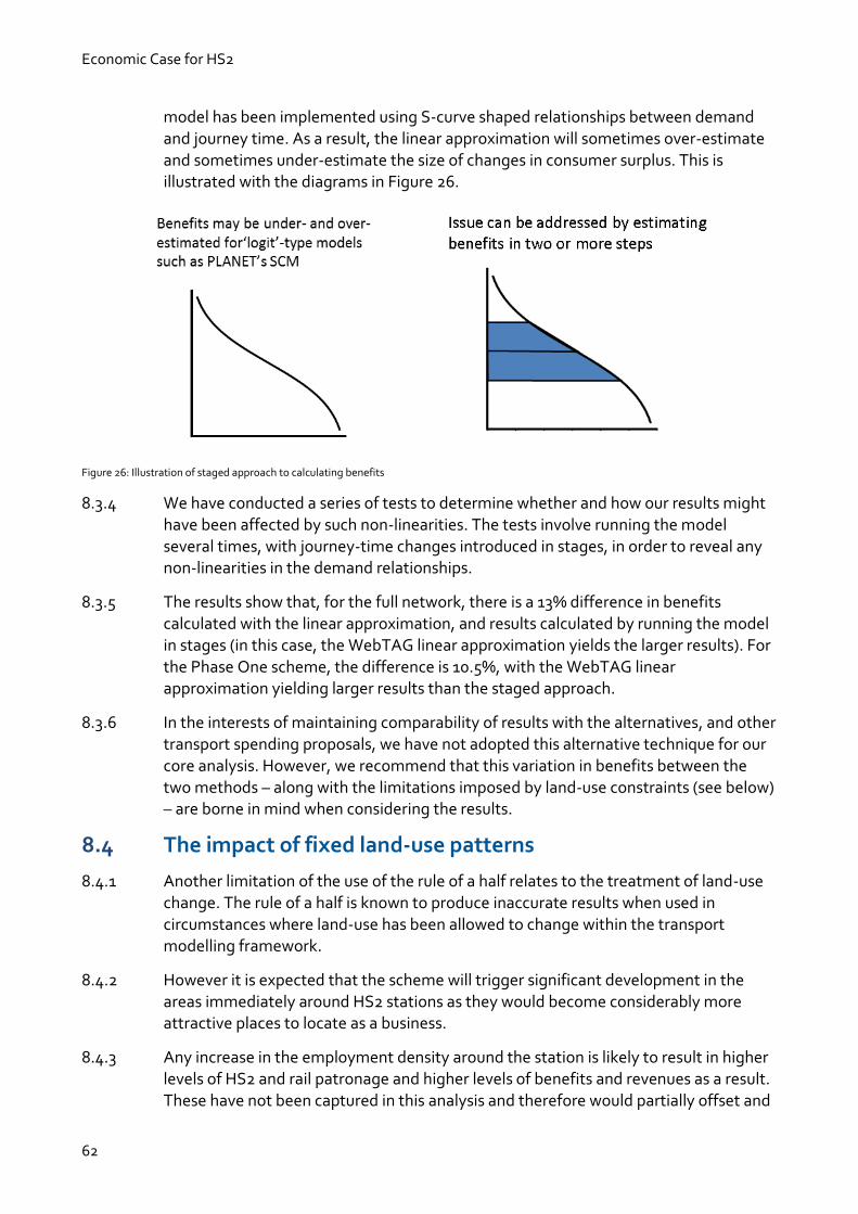
Economic Case for HS2
62
model has been implemented using S-curve shaped relationships between demand
and journey time. As a result, the linear approximation will sometimes over-estimate and sometimes under-estimate the size of changes in consumer surplus. This is illustrated with the diagrams in Figure 26.
Figure 26: Illustration of staged approach to calculating benefits
8.3.4 We have conducted a series of tests to determine whether and how our results might have been affected by such non-linearities. The tests involve running the model several times, with journey-time changes introduced in stages, in order to reveal any non-linearities in the demand relationships.
8.3.5 The results show that, for the full network, there is a 13% difference in benefits calculated with the linear approximation, and results calculated by running the model in stages (in this case, the WebTAG linear approximation yields the larger results). For the Phase One scheme, the difference is 10.5%, with the WebTAG linear approximation yielding larger results than the staged approach.
8.3.6 In the interests of maintaining comparability of results with the alternatives, and other
transport spending proposals, we have not adopted this alternative technique for our core analysis. However, we recommend that this variation in benefits between the two methods – along with the limitations imposed by land-use constraints (see below) – are borne in mind when considering the results.
8.4 The impact of fixed land-use patterns
8.4.1 Another limitation of the use of the rule of a half relates to the treatment of land-use change. The rule of a half is known to produce inaccurate results when used in circumstances where land-use has been allowed to change within the transport modelling framework.
8.4.2 However it is expected that the scheme will trigger significant development in the areas immediately around HS2 stations as they would become considerably more attractive places to locate as a business.
8.4.3 Any increase in the employment density around the station is likely to result in higher levels of HS2 and rail patronage and higher levels of benefits and revenues as a result. These have not been captured in this analysis and therefore would partially offset and

Economic Case for HS2
63
potentially outweigh the difference between the rule of a half and the alternative numerical integration method
8.4.4 On this basis, and also the need to ensure comparability of results, we have not deviated from the WebTAG guidance, and have continued to use the standard rule of a half approximation for the calculation of consumer surplus. This may result in the under- or over-estimation of benefits, and we will conduct further analysis to better understand the balance of the two effects.

Economic Case for HS2
64
Appendices
1 Modelling and appraisal approach 1.1 PLANET modelling
1.1.1 Our modelling approach utilises the PLANET Framework Model (PFM), a detailed description of which is provided in PLANET framework model (PFM v4.3) – Model Description. Its main aim is to provide forecasts of demand to drive the appraisal of HS2.
1.1.2 PFM works by splitting Great Britain into 235 zones. Using current costs and travel statistics it is able to model the present demand for journeys between each zone by road, rail and air. By looking at the historic rate of demand growth for each mode of
transport and many other factors we can predict future journey patterns using the current infrastructure. As a final step we can introduce HS2 and model how this will cause the demand for each mode of transport to change and how many people will want to use HS2.
1.1.3 The future prediction without HS2 represents the 'Do Minimum' option and the predictions with HS2 are the 'Do Something' options. The difference between the 'Do Minimum' and the 'Do Something' tells us the impact that HS2 will have.
1.1.4 Within PFM the emphasis is mainly on longer distance movements. The main area where shorter distance movements need to be represented is for rail, in order to reflect potential reductions of crowding on local services. To combine the impact of long-distance and short-distance trips PFM is actually made up of four models, one
specialises in looking at long-distance trips, the other three focusing in detail on the south, Midlands and the North of the UK.
1.1.5 Forecasts are made separately for three modes (rail, car, air), and the required input variables or 'demand drivers' vary between them, with the rail forecasts being the most detailed. Common to all three modes is a consistent set of assumptions relating to the following demand drivers:
Population – we assume that the population of Great Britain grows by 14.9%
between 2010 and 2036, which is a revised estimate based on ONS low migration projections from October 2011.
Employment – we assume that employment in GB grows by 12.4% between 2010 and 2036, which is a revised estimate based on OBR national forecasts (March 2012 for short-term forecasts and July 2012 for long term forecasts).
GDP per capita – we assume that the British GDP per capita grows by 52% between 2010 and 2036, which is a revised estimate based on OBR national forecasts (March 2012 for short-term forecasts and July 2012 for long term forecasts).
1.1.6 A review has been undertaken to ensure that all planned future investments and changes to current infrastructure are also included in the model at the time that they

Economic Case for HS2
65
are planned to be implemented. It is important to include all planned infrastructure
investments in the ‘Do Something’ option, so that HS2 is modelled in the most realistic way. These planned interventions are outlined in section 1.3. In the case of rail, this included an assessment of service and journey time improvements identified by the DfT and the operators. Information relating to the proposed enhancements to the highway network between 2010 and 2026 has been provided by the DfT’s national transport model’s list of schemes. This was reviewed against lists on the Highways Agency’s Road Projects website (and Welsh and Scottish equivalents), the National Infrastructure Plan 2011 and subsequent DfT announcements.
1.2 Updates to our approach
1.2.1 Over the last year, PFM has undergone significant development and updating in response to the latest evidence and a review undertaken by independent experts and our Analytical Challenge Panel. This has resulted in a number of key changes.
Revised demand forecasts
1.2.2 We have updated our assessment of how demand will change in the future. Since the previous economic case the DfT has revised its WebTAG guidance so that the relationship between growth in rail demand and economic growth and other drivers is based on PDFH version 5. In line with WebTAG, the relationship between fares and growth continues to be based on PDFH version 4.
1.2.3 Our forecasts of Gross Domestic Product (GDP) growth have been updated to be in line with Office of Budget Responsibility (OBR) forecasts from July 2012. Our forecasts of other drivers of demand such as population, and the cost and time of travelling by other modes has also been updated in line with DfT guidance. All rail fares are assumed to increase at RPI+1 per year until the cap year.
1.2.4 There have been very recent updates of medium term GDP growth in March 2013 and long term GDP growth in July 2013. These updates were made too late to be included in the analysis but our risk analysis around GDP growth uses simulation tests that have rates of growth similar to these updates.
1.2.5 To better understand how people currently make long-distance highway trips, we have incorporated new evidence available from the Department for Transport’s Long-Distance Model and National Travel Survey. Our highway forecasts were also updated to use the same GDP forecasts as above.
1.2.6 Air forecasts have been updated using data from the DfT's National Air Passenger Allocation Model (NAPALM).
1.2.7 The result of these changes is that we now forecast slightly faster growth in long-distance rail trips for the standard case. As discussed in section 6 of the main document, demand growth is capped in the standard case. As there is now faster growth this takes place in 2036 rather than 2037.
Updates and improvements to appraisal
The Department for Transport has made a number of changes to its WebTAG 1.2.8guidance which our modelling now incorporates. These include the following:

Economic Case for HS2
66
Revised value of time. The DfT have, alongside this report, published new
values of time (VoT) in draft WebTAG guidance for use in transport analysis. We have adopted the new draft values in anticipation. This reduces benefits attributable to business travellers but increases the benefits attributable to commuting and leisure passengers. The method by which VoT is grown over time has also been revised. VoT is one of the key factors in our analysis and is explored in more detail in Chapter 5.
Costs and benefits are presented in 2011 prices using the Office of National Statistics GDP deflator as a measure of inflation. The definition of this deflator has been changed from being more consistent with a Retail Price Index (RPI) to a Consumer Price Index (CPI) metric. As fares increase in line with RPI, this means that in real terms, our RPI+1% fares assumption results in increased revenue.
1.2.9 We have also made a number of changes to bring our modelling more closely in line with WebTAG guidance including:
Business crowding and boarding or interchange impacts are now assessed using business values of time rather than commuting values of time.
The method by which the model calculates the economic benefits of changes in demand and journey times has been changed to be more consistent with WebTAG. The calculation of benefits is now carried out at the most disaggregate level possible before being summed.
Updates to the modelling approach
1.2.10 The demand model that determines how passengers will react to the new journey
opportunities resulting from HS2 has been re-calibrated to better reflect observed behaviour. While the previous model was calibrated in part on the basis of expert judgement, the model is now based on data from the National Travel Survey and improves consistency in WebTAG. The result is that generally the amount of demand forecast to switch from alternative modes onto HS2 reduces, although the amount of demand that is generated by new trips increases. Overall this results in a slight reduction in the number of forecast HS2 passengers.
1.2.11 The method by which the model determines which trains passengers choose to travel on has been improved, so that it now takes account of journey time and crowding impacts as well as frequency.
1.2.12 Improvements to how different elements of the framework interact with one another
have been made, including a better understanding of the proportion of daily demand that occurs in the peak.
1.2.13 Improvements in understanding the accessibility of stations that ensures we are consistent in our assumptions on the provision of local transport schemes with organisations such as TfL have been incorporated.
1.2.14 To produce better forecasts of future demand patterns, HS2 Ltd has undertaken research on existing demand patterns. In particular, we have focused on better
Economic Case for HS2
67
understanding the journey purpose of current rail passengers and whether they are categorised as business, leisure or commuting.
1.2.15 Our previous approach for determining this journey purpose made use of the National Rail Travel Survey (NRTS)29 to derive a relationship between the type of ticket that was sold and the purpose of the journey. This was based on a single national average and meant our assumptions on journey purpose showed little variation between different places in the country.
1.2.16 Moreover, analysis of other data sources such as the National Passenger Survey (NPS)30 has shown that while the journey purpose mix has remained stable since the NRTS was undertaken, the relationship between ticket type and journey purpose has changed, in part due to the greater availability of discounted tickets.
1.2.17 In this updated economic analysis we have therefore avoided the use of a ticket type
relationship, and instead used the NRTS to directly estimate the journey purposes mix for different flows. This means that the journey purpose mix is now entirely consistent with NRTS; and shows the same regional variation. It also means our journey purpose
assumptions are consistent with version 5 of the Passenger Demand Forecasting Handbook which is based on the same NRTS data, and which has been adopted by the Department for Transports in its WebTAG guidance.
Updates to the ‘without scheme’ baseline
1.2.18 Our modelling is dependant on comparing the impact of HS2 with the alternative of not building HS2. If HS2 is not built there will still be growth in long-distance rail travel and there will also be some investment that is already planned for the current rail network. It is therefore important that we maintain an up to date 'Do Minimum' option so that we can accurately compare HS2 with the alternative future.
1.2.19 Since August 2012 there have been a number of updates to the ‘Do Minimum’ option including:
incorporation of electrification of the Midland Main Line from St Pancras involving increased capacity and faster journey times to the East Midlands;
incorporation of Intercity Express Rolling Stock on the East Coast Main Line resulting in increased capacity and faster journey times;
improvements to the West Coast Main Line potential service specification that makes use of additional train paths, faster running speeds and infrastructure improvements. These changes result in additional services, increased capacity and faster journey times;
29 National rail travel survey overview report - https://www.gov.uk/government/publications/national-rail-travel-survey-overview-report 30 National Passenger Survey (NPS) - http://www.passengerfocus.org.uk/research/national-passenger-survey-introduction

Economic Case for HS2
68
incorporation of the Northern Hub scheme to provide faster and more
frequent services across the north of England; and
inclusion of East-West Rail scheme between Oxford and Milton Keynes which will facilitate new local services and faster cross-country services.
Economic Case for HS2
69
2 Scheme assumptions and service patterns
2.1 Phase One
2.1.1 There will be four stations on the Phase One route; Birmingham Curzon Street, Birmingham Interchange, Old Oak Common and London Euston. Phase One would also include a link to HS1 north of Euston and St Pancras. All the stations except Euston are designed to be capable of handling international passengers.
2.1.2 Phase One includes the longest section of track without a station between Old Oak Common and Birmingham Interchange. This section will be capable of handling 18 trains per hour in each direction and is expected to carry 138,000 passengers a day
from 2036. This will rise to over 240,000 passengers a day in 2036 once the full network is complete.
2.2 Phase Two and the full network
2.2.1 Since the August 2012 Economic Update plans for the full network have been developed considerably. A consultation of the preferred route for Phase Two was launched on 17 July 2013. Phase One and Phase Two together will form the full Hs2 network which is the extent of the high-speed network that is currently being considered.
2.2.2 A decision on the Government’s preferred route for Phase Two is expected by the end of 2014. For this analysis we have assumed the proposed route that was released for public consultation on 17 July 2013.
2.3 HS2 service patterns
2.3.1 Figure 27 shows the HS2 service pattern for Phase One. This includes changes to bring the service pattern in line with the Full Network service pattern. Figure 28 shows the Full Network service pattern. As mentioned in chapter 3 this has resulted in some changes to the splitter service. This was previously assumed to serve Birmingham and Liverpool, but has now been switched to the eastern leg. Stops have also been added on the Scottish and Newcastle services.
2.4 Released capacity service patterns
2.4.1 Assumptions about released capacity are required for our modelling. What is used represents one possible set of assumptions for business case modelling purposes.
There are many other potential combinations of released capacity. Much more work will be needed to determine actual train service specifications for a point in 15 to 20 years time. The assumptions made for this update of the economic case are set out in the PFM V4.3: Assumptions Report.

Economic Case for HS2
70
2.5 Freight
2.5.1 Though rail freight will not use HS2, the capacity released by migration of passengers onto a new high speed line will mean that more rail freight can be moved on the major north-south rail routes. Not only would the increased availability for freight benefit businesses but it is also likely that it would remove heavy goods vehicles from the motorways reducing congestion and carbon emissions.
2.5.2 The economic case does not make any assumptions about the potential use of released capacity for more freight movements than under the current timetable (current freight paths are preserved in the modelled service specification). This is a conservative assumption; additional freight capacity should generate additional carbon and other benefits from the scheme that could be added to the case. Current work shows that capacity released by HS2 should enable at least 10 freight paths per
day from London to the West Midlands in each direction, giving at least 20 additional freight paths per day. More freight paths may become available during the course of timetable development, and would provide further benefits.
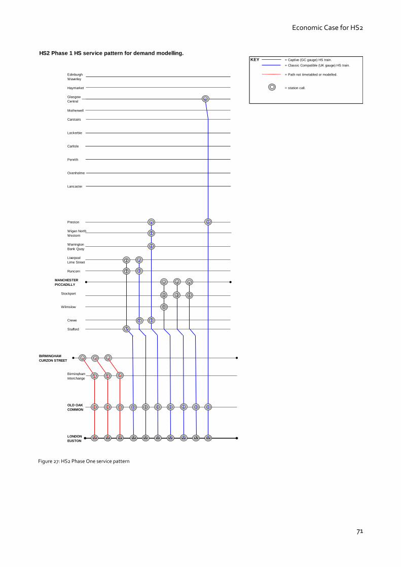
Economic Case for HS2
71
Figure 27: HS2 Phase One service pattern
HS2 Phase 1 HS service pattern for demand modelling.KEY = Captive (GC gauge) HS train.
= Classic Compatible (UK gauge) HS train.
Edinburgh = Path not timetabled or modelled.
Waverley
Haymarket = station call.
Glasgow
Central
Motherwell
Carstairs
Lockerbie
Carlisle
Penrith
Oxenholme
Lancaster
Preston
Wigan North
Western
Warrington
Bank Quay
Liverpool
Lime Street
Runcorn
MANCHESTER
PICCADILLY
Stockport
Wilmslow
Crewe
Stafford
BIRMINGHAM
CURZON STREET
Birmingham
Interchange
OLD OAK
COMMON
LONDON
EUSTON
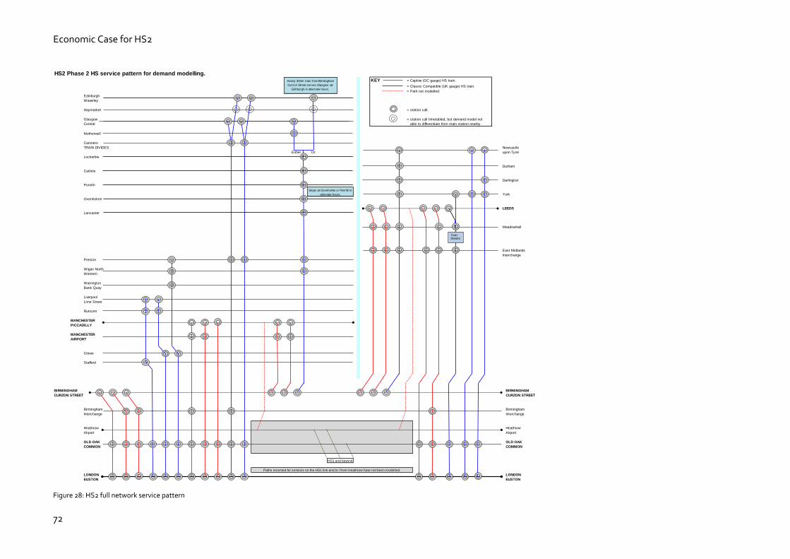
Economic Case for HS2
72
Figure 28: HS2 full network service pattern
HS2 Phase 2 HS service pattern for demand modelling.KEY = Captive (GC gauge) HS train.
= Classic Compatible (UK gauge) HS train.
= Path not modelled.
Edinburgh
Waverley
Haymarket = station call.
Glasgow = station call timetabled, but demand model not
Central able to differentiate from main station nearby.
Motherwell Prepared by Jeff Hawken
HS2 Operations Planning Manager
Carstairs
TRAIN DIVIDES Newcastle
Either Or upon Tyne
Lockerbie
Durham
Carlisle
Darlington
Penrith
York
Oxenholme
LEEDS
Lancaster
Meadowhall
East Midlands
Interchange
Preston
Wigan North
Western
Warrington
Bank Quay
Liverpool
Lime Street
Runcorn
MANCHESTER
PICCADILLY
MANCHESTER
AIRPORT
Crewe
Stafford
BIRMINGHAM BIRMINGHAM
CURZON STREET CURZON STREET
Birmingham Birmingham
Interchange Interchange
Heathrow Heathrow
Airport Airport
OLD OAK OLD OAK
COMMON COMMON
LONDON LONDON
EUSTON EUSTON
Hourly 200m train from Birmingham
Curzon Street serves Glasgow or
Edinburgh in alternate hours.
HS1 and beyond
Paths reserved for services on the HS1 link and to / from Heathrow have not been modelled.
Stops at Oxenholme or Penrith in
alternate hours.
Train Divides

Economic Case for HS2
73
3 Cost assumptions 3.1 Overview
3.1.1 Costs are calculated in three primary groups outlined below and then combined to give the net cost to Government. Costs have been calculated in 2011 prices to remain consistent with the rest of the economic analysis. For more information on the development of the cost estimating see the HS2 Cost and Risk Status Report.
Capital costs - Including land purchase, design, materials and construction
Rolling stock – design and purchase
Operating costs - Including operation and maintenance of train and track, train crew and station staff for HS2 and any operating cost savings from changes to the classic network.
3.1.2 These costs are then offset by any generated revenue from HS2 or the classic network to generate the net cost to government. This is the amount that HS2 is expected to cost over the appraisal period. It consists of all the capital and operating costs summed together, minus the generated revenue. It is the value that is used as the total cost of the scheme for the calculation of the BCR.
3.1.3 The two phases of the scheme are at different stages in the delivery process. There is therefore a difference in design maturity and the process behind building the estimate reflects this.
3.1.4 Lessons have been learnt for the process with Phase One, and will have improved the initial accuracy of the cost estimates for Phase Two. For example we have revised our land and property costs.
3.1.5 A key objective for the future will be to reduce the planned costs of the project through value engineering and identifying efficiencies. The Efficiency Challenge Programme has been set up to identify and realise cost savings. As the design of the project becomes more detailed, it may be possible to reduce the significant allowances for optimism bias in the estimated costs. Reducing the overall project cost will increase the BCR and the project's value for money.
3.2 Construction costs
3.2.1 The cost estimate for construction has been prepared by a number of the construction industry’s leading engineering consultancies, supported by quantity surveyors and
contractors. The construction cost estimates also include advanced works, third party costs, contractor's preliminaries and overheads. Risk is also included but at different levels depending on the scenario being considered.
3.2.2 Extensive design development has utilised more accurate survey work and included elements such as road diversions that had not been designed before. There has also been development of plans identifying how the railway will be constructed and how environmental impact mitigation measures will be implemented.
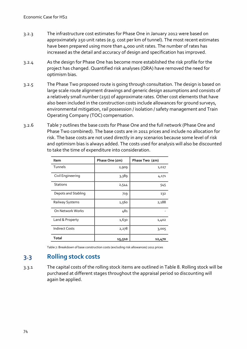
Economic Case for HS2
74
3.2.3 The infrastructure cost estimates for Phase One in January 2012 were based on
approximately 250 unit rates (e.g. cost per km of tunnel). The most recent estimates have been prepared using more than 4,000 unit rates. The number of rates has increased as the detail and accuracy of design and specification has improved.
3.2.4 As the design for Phase One has become more established the risk profile for the project has changed. Quantified risk analyses (QRA) have removed the need for optimism bias.
3.2.5 The Phase Two proposed route is going through consultation. The design is based on large scale route alignment drawings and generic design assumptions and consists of a relatively small number (250) of approximate rates. Other cost elements that have also been included in the construction costs include allowances for ground surveys, environmental mitigation, rail possession / isolation / safety management and Train Operating Company (TOC) compensation.
3.2.6 Table 7 outlines the base costs for Phase One and the full network (Phase One and Phase Two combined). The base costs are in 2011 prices and include no allocation for
risk. The base costs are not used directly in any scenarios because some level of risk and optimism bias is always added. The costs used for analysis will also be discounted to take the time of expenditure into consideration.
Item Phase One (£m) Phase Two (£m)
Tunnels 2,909 1,027
Civil Engineering 3,389 4,171
Stations 2,544 545
Depots and Stabling 719 132
Railway Systems 1,560 2,188
On Network Works 481 -
Land & Property 1,630 1,402
Indirect Costs 2,278 3,005
Total 15,510 12,470
Table 7: Breakdown of base construction costs (excluding risk allowances) 2011 prices
3.3 Rolling stock costs
3.3.1 The capital costs of the rolling stock items are outlined in Table 8. Rolling stock will be
purchased at different stages throughout the appraisal period so discounting will again be applied.

Economic Case for HS2
75
Item Train Cost Required for
Phase One
Total required
for full network
Standard Case
Optimism Bias
Captive fleet £26.5 Million 24 81 15%
Classic-compatible fleet £30.5 million 44 99 20%
Design of all trains £420 million 1 1 100%
Table 8: Breakdown of rolling stock costs (2011 prices)
3.3.2 There will be two different types of train in operation on the HS2 network. Classic-compatible trains will be designed to be capable of using both high-speed track and the current rail network. This will allow direct services to run from London to cities north of Birmingham after completion of Phase One, and north of Leeds and
Manchester after the completion of the full network. These services will gain a time saving for the part of the journey that is on high speed track and then run at conventional speed on the classic track.
3.3.3 Optimism bias has been applied to allow for the unpredictability of tendering rolling stock production in the future. There is significant uncertainty in the estimates for the design costs and therefore a very high level of optimism bias is applied. The cost of the rolling stock has been kept the same for all scenarios so the costs below are used in all scenarios.
Phase One only Rolling stock cost – £3.2 billion in 2011 prices
Full Network rolling stock cost – £6.9 billion in 2011 prices
3.3.4 As the same design of trains will be used for Phase One and Phase Two the design cost of all trains needs only be incurred once. The design cost has been attributed to Phase One so there is no design cost for Phase Two.
3.3.5 The work described in this section was concluded and validated after the conclusion of the Spending Round. Therefore, these numbers are slightly different to those used for spending round conclusions. More detail can be found in the HS2 cost and risk model report.
3.4 Infrastructure and rolling stock renewals
3.4.1 There will be a capital renewal allowance for investment in the infrastructure during the life of the assets. Painting, cleaning and general maintenance of the infrastructure will be covered by operating costs but larger expenditures such as repairs and replacements will require capital expenditure.
3.4.2 The cost of the infrastructure renewals has been kept the same for all scenarios so the costs below are used in all scenarios.
Phase One only infrastructure renewals cost – £1.4 billion in 2011 PV.
Full network infrastructure renewals cost – £2.4 billion in 2011 PV.

Economic Case for HS2
76
3.4.3 It is also assumed that all the rolling stock costs including the design will be incurred
twice. This is because the trains have an expected life of 35 years and will need replacing once during the appraisal period. When the trains are replaced, it is anticipated that a complete redesign will be required to make use of the most up to date technologies and best practice.
3.5 Quantified Risk Assessment
3.5.1 A quantitative risk assessment (QRA) is used to determine the level of contingency that should be added to the base cost estimate.
3.5.2 The QRA includes threats that may or may not occur and tolerance ranges associated with the status of the price estimation and design development. Both threats and tolerances represent uncertainty to the base cost estimate.
3.5.3 The base cost estimate was generated from bottom-up design and cost information, and represents a ‘most likely winning tender’ price. It includes assumptions about scope and rates; assumptions about potential value engineering savings; and assumptions about potential efficiency savings.
3.5.4 The QRA uses stochastic modelling to allow the cost uncertainties to be represented by ranges rather than single values, and the inclusion of events that may or may not occur. Each input is assigned one or more representative probability distributions which are sampled when the simulation is run.
3.5.5 A simulation consists of a large number of re-calculations (iterations) of the cost estimate. For each iteration, a single cost is sampled from the range of possible costs for each item (tolerance or threat) included in the model. The sampled cost values are added together to give one possible value of the project’s total cost. This total cost is
saved and the next iteration is calculated with a different set of samples, and so on until enough iterations have been performed to allow the ‘basket’ of possible total costs to stabilise statistically.
3.5.6 The simulation produces a range of possible total costs which are usually presented as a cumulative frequency distribution, or s-curve. The s-curve shows the probability that a given cost will not be exceeded. P50 and P95 costs are typical quoted values from the s-curve. P50 is short-hand for the 50th percentile. The P50 cost is the cost for which there is a 50% chance of not being exceeded. The P95 cost has a 95% chance of not being exceeded.
3.6 Operating costs
3.6.1 All operating cost inputs and assumptions have gone through a comprehensive review to verify whether they are the most appropriate inputs to estimate the various costs, and to update in line with new or more detailed data where appropriate.

Economic Case for HS2
77
3.6.2 The operating cost changes that have had the largest impacts are:
Train electricity consumption: detailed modelling of the energy consumption
of HS2’s reference train based on a range of evidence including the RailPlan tool developed by Trapeze Group31 tool has significantly changed our estimates of the amount of energy consumed by HS2 trains on the captive network; and
TOC overheads and admin: we have used significantly more detailed data on TOC operating costs to enable a better estimation of this cost.
3.6.3 In light of more detailed information, we have also added two new cost items to the model – the cost of HS2’s impact on the classic line stations that they call at, and the cost of running an infrastructure manager head office.
3.6.4 We apply optimism bias to our estimates of operational expenditure to allow for the risk of underestimating costs. In previous economic cases, we have used an OB rate of 41% for all non-lease costs, and 18% for lease costs for a cautious allowance which is in line with the DfT’s Strategic Alternatives.
3.6.5 In consultation with DfT, we have now moved to a model whereby the level of OB we apply to each operating cost line is dependent on the quality of the data our estimate is based on, and the maturity of the cost estimate. Each operating cost line now has a tailored OB rate between 10% and 41%.
3.6.6 We now no longer apply OB to our estimate of savings on the classic line.
3.6.7 Table 9 outlines the operating costs for Phase One and the full network. The operating costs have been kept the same for all scenarios so the costs below are used in all scenarios.
31Trapeze group – http://www.trapezegroup.co.uk/solutions/rail-planning/simulation-of-train-operations

Economic Case for HS2
78
Item Phase One (£m) Full Network (£m) Includes
Rolling stock
maintenance
3,486 8,964 Clearing, repairing and servicing the trains
Infrastructure
maintenance
1,454 2,931 Inspecting and repairing the infrastructure, and
Infrastructure manager head office
Electrical consumption 2,210 6,055 Cost of electricity used by the trains and electrification
asset usage charge
Staff, offices and
stations
5,957 11,200 Station Staff , Station Maintenance & Utilities, Train
Crew, TOC overheads and Admin including head office
staff
Other 732 1,258 Variable tack access charge, Capacity charge, station
access charge and rolling stock insurance
Classic line savings -5,675 -8,265 Staff, electricity, diesel, lease costs, maintenance and
other
Total 8,166 22,143 All costs net of classic line savings
Table 9: Breakdown of operating costs (2011 prices present value including Optimism Bias)
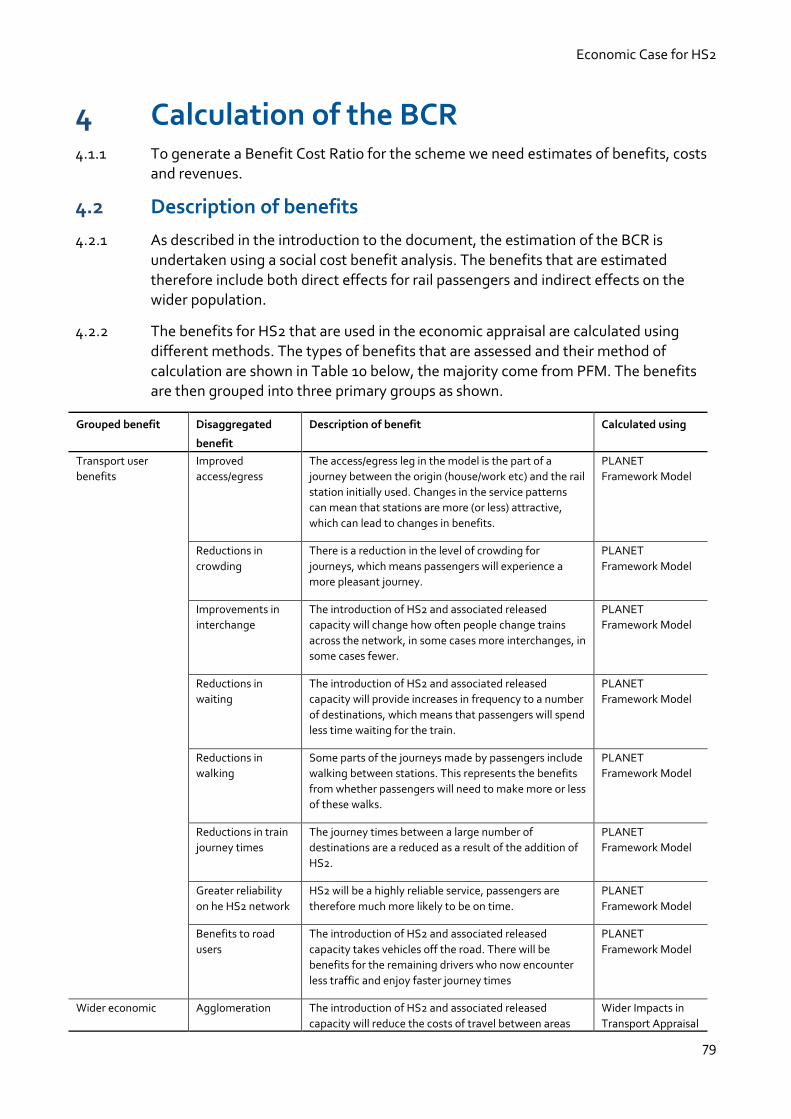
Economic Case for HS2
79
4 Calculation of the BCR 4.1.1 To generate a Benefit Cost Ratio for the scheme we need estimates of benefits, costs
and revenues.
4.2 Description of benefits
4.2.1 As described in the introduction to the document, the estimation of the BCR is undertaken using a social cost benefit analysis. The benefits that are estimated therefore include both direct effects for rail passengers and indirect effects on the wider population.
4.2.2 The benefits for HS2 that are used in the economic appraisal are calculated using different methods. The types of benefits that are assessed and their method of
calculation are shown in Table 10 below, the majority come from PFM. The benefits are then grouped into three primary groups as shown.
Grouped benefit Disaggregated
benefit
Description of benefit Calculated using
Transport user
benefits
Improved
access/egress
The access/egress leg in the model is the part of a
journey between the origin (house/work etc) and the rail
station initially used. Changes in the service patterns
can mean that stations are more (or less) attractive,
which can lead to changes in benefits.
PLANET
Framework Model
Reductions in
crowding
There is a reduction in the level of crowding for
journeys, which means passengers will experience a
more pleasant journey.
PLANET
Framework Model
Improvements in
interchange
The introduction of HS2 and associated released
capacity will change how often people change trains
across the network, in some cases more interchanges, in
some cases fewer.
PLANET
Framework Model
Reductions in
waiting
The introduction of HS2 and associated released
capacity will provide increases in frequency to a number
of destinations, which means that passengers will spend
less time waiting for the train.
PLANET
Framework Model
Reductions in
walking
Some parts of the journeys made by passengers include
walking between stations. This represents the benefits
from whether passengers will need to make more or less
of these walks.
PLANET
Framework Model
Reductions in train
journey times
The journey times between a large number of
destinations are a reduced as a result of the addition of
HS2.
PLANET
Framework Model
Greater reliability
on he HS2 network
HS2 will be a highly reliable service, passengers are
therefore much more likely to be on time.
PLANET
Framework Model
Benefits to road
users
The introduction of HS2 and associated released
capacity takes vehicles off the road. There will be
benefits for the remaining drivers who now encounter
less traffic and enjoy faster journey times
PLANET
Framework Model
Wider economic Agglomeration The introduction of HS2 and associated released
capacity will reduce the costs of travel between areas
Wider Impacts in
Transport Appraisal

Economic Case for HS2
80
impacts benefits and businesses which will lead to greater business
interaction
model
Imperfect
competition
Companies will be able to increase their production as a
result of lower transport costs
Wider Impacts in
Transport Appraisal
model
Increased labour
force participation
Transport changes can affect the individual incentives
to work and therefore affect the overall level of labour
supply
Wider Impacts in
Transport Appraisal
model
Other impacts Reduction of car
noise
The introduction of HS2 and associated released
capacity takes cars off the road, so there will less noise
caused by cars
PLANET
Framework Model
Carbon The introduction of HS2 and associated released
capacity will reduce the total distance cars and diesel
trains travel each year, which will reduce the carbon
emissions they produce
Spreadsheet Model
HS1 link HS2 will be linked to HS1 and this will allow improved
services to Continental Europe for passengers using HS2
International
Demand Model
Reduction in car
accidents
The introduction of HS2 and associated released
capacity reduces the total number of cars on the road
there will fewer car accidents
PLANET
Framework Model
Noise from HS2
trains
HS2 trains will create noise and this will have a negative
impact on areas close to the track
Spreadsheet Model
Tax impacts Loss to
government of
indirect tax
As there will be fewer passengers travelling by car or
other means, there will be a reduction in the level of tax
generated as a result.
PLANET
Framework Model
Table 10: Grouped and disaggregated benefits, what they are and where they are calculated
4.2.3 The estimates of benefits are then combined to provide an estimate of net benefits:
Net benefits = Transport User benefits + WEIs + Other impacts + Tax Impacts
4.3 Costs and revenue
4.3.1 As set out in Appendix 3 costs are estimated for three primary groups: construction, rolling stock and operating costs. Operating costs includes both the costs of operating HS2 trains and savings from changes to services on the classic network. The costs of renewals are also included.
4.3.2 Revenue is estimated using changes in passenger km from the PFM model, again incorporating changes from both HS2 and classic line passengers.

Economic Case for HS2
81
4.3.4 These estimates of cost and revenue are then combined to give a net cost to Government:
Net cost to Government =
Construction cost + rolling stock cost + operating cost + renewals – revenue
4.4 Calculation of the BCR
4.4.1 All the estimates of the benefits and costs are then combined in the following equation to produce an estimate of the BCR.
BCR = Net benefits
Net Cost to Government
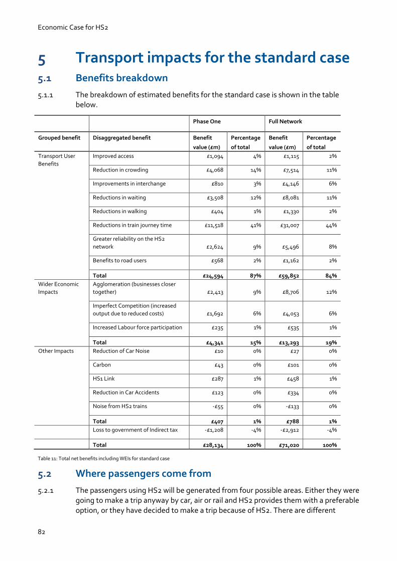
Economic Case for HS2
82
5 Transport impacts for the standard case 5.1 Benefits breakdown
5.1.1 The breakdown of estimated benefits for the standard case is shown in the table below.
Phase One Full Network
Grouped benefit Disaggregated benefit Benefit
value (£m)
Percentage
of total
Benefit
value (£m)
Percentage
of total
Transport User
Benefits
Improved access £1,094 4% £1,115 2%
Reduction in crowding £4,068 14% £7,514 11%
Improvements in interchange £810 3% £4,146 6%
Reductions in waiting £3,508 12% £8,081 11%
Reductions in walking £404 1% £1,330 2%
Reductions in train journey time £11,518 41% £31,007 44%
Greater reliability on the HS2
network £2,624 9% £5,496 8%
Benefits to road users £568 2% £1,162 2%
Total £24,594 87% £59,852 84%
Wider Economic
Impacts
Agglomeration (businesses closer
together) £2,413 9% £8,706 12%
Imperfect Competition (increased
output due to reduced costs) £1,692 6% £4,053 6%
Increased Labour force participation £235 1% £535 1%
Total £4,341 15% £13,293 19%
Other Impacts Reduction of Car Noise £10 0% £27 0%
Carbon £43 0% £101 0%
HS1 Link £287 1% £458 1%
Reduction in Car Accidents £123 0% £334 0%
Noise from HS2 trains -£55 0% -£133 0%
Total £407 1% £788 1%
Loss to government of Indirect tax -£1,208 -4% -£2,912 -4%
Total £28,134 100% £71,020 100%
Table 11: Total net benefits including WEIs for standard case
5.2 Where passengers come from
5.2.1 The passengers using HS2 will be generated from four possible areas. Either they were going to make a trip anyway by car, air or rail and HS2 provides them with a preferable option, or they have decided to make a trip because of HS2. There are different

Economic Case for HS2
83
amounts of benefits for each passenger depending on why the passenger has chosen
to use HS2 and it is therefore important for us to understand where the passengers have come from.
5.2.2 For the standard case the passengers for the full network will come from the four possible areas in the percentages shown in Table 12.
Full network (2036)
Switching from classic rail 69%
New trips 26%
Shift from air 1%
Shift from car 4%
Total 100%
Table 12: Breakdown of where passengers will be generated from
5.3 Regional benefits
5.3.1 Using the standard case Table 13 shows the distribution of benefits according to where a trip starts. The figures are the total values of the transport user benefits in that area in 2036 only.
Region Phase One (2036) Full network (2036)
London 42% (£339) 35% (£726)
South East 3% (£22) 3% (£58)
West Midlands 26% (£211) 15% (£303)
North West 20% (£164) 17% (£342)
East Midlands 2% (£15) 8% (£157)
Yorkshire and Humber 1% (£6) 11% (£225)
North East 0% (£1) 3% (£69)
Scotland 2%( £19) 4% (£91)
Other (East England, South West, Wales) 4% (£31) 4% (£76)
Total 100% (£809) 100% (£2,047)
Table 13: Regional distribution of transport user benefits (value in brackets are in £millions)
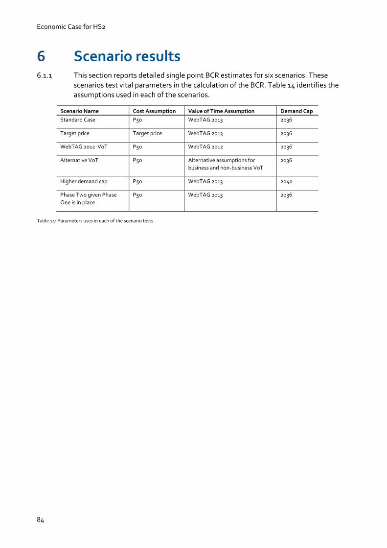
Economic Case for HS2
84
6 Scenario results 6.1.1 This section reports detailed single point BCR estimates for six scenarios. These
scenarios test vital parameters in the calculation of the BCR. Table 14 identifies the assumptions used in each of the scenarios.
Scenario Name Cost Assumption Value of Time Assumption Demand Cap
Standard Case P50 WebTAG 2013 2036
Target price Target price WebTAG 2013 2036
WebTAG 2012 VoT P50 WebTAG 2012 2036
Alternative VoT P50 Alternative assumptions for
business and non-business VoT
2036
Higher demand cap P50 WebTAG 2013 2040
Phase Two given Phase
One is in place
P50 WebTAG 2013 2036
Table 14: Parameters uses in each of the scenario tests

Economic Case for HS2
85
6.2 Standard case
6.2.1 The standard case scenario uses all the WebTAG standard assumptions.
BCR Components Phase One (£billion) Full Network (£billion)
1
Transport user benefits
Business £16.9 £40.5
Other £7.7 £19.3
2 Other quantifiable benefits £0.4 £0.8
3 Loss to Government of indirect taxes -£1.2 -£2.9
4 Net transport benefits = (1) + (2) + (3) £23.8 £57.7
5 Wider economic impacts (WEIs) £4.3 £13.3
6 Net benefits including WEIs = (4) + (5) £28.1 £71.0
7 Capital costs £21.8 £40.5
8 Operating costs £8.2 £22.1
9 Total costs = (7) + (8) £29.9 £62.6
10 Revenues £13.2 £31.1
11 Net costs to Government = (9) – (10) £16.7 £31.5
12 BCR without WEIs (ratio) = (4)/(11) 1.4 1.8
13 BCR with WEIs (ratio) = (6)/(11) 1.7 2.3
Table 15: Economic analysis results for the standard case scenario (2011 PV)
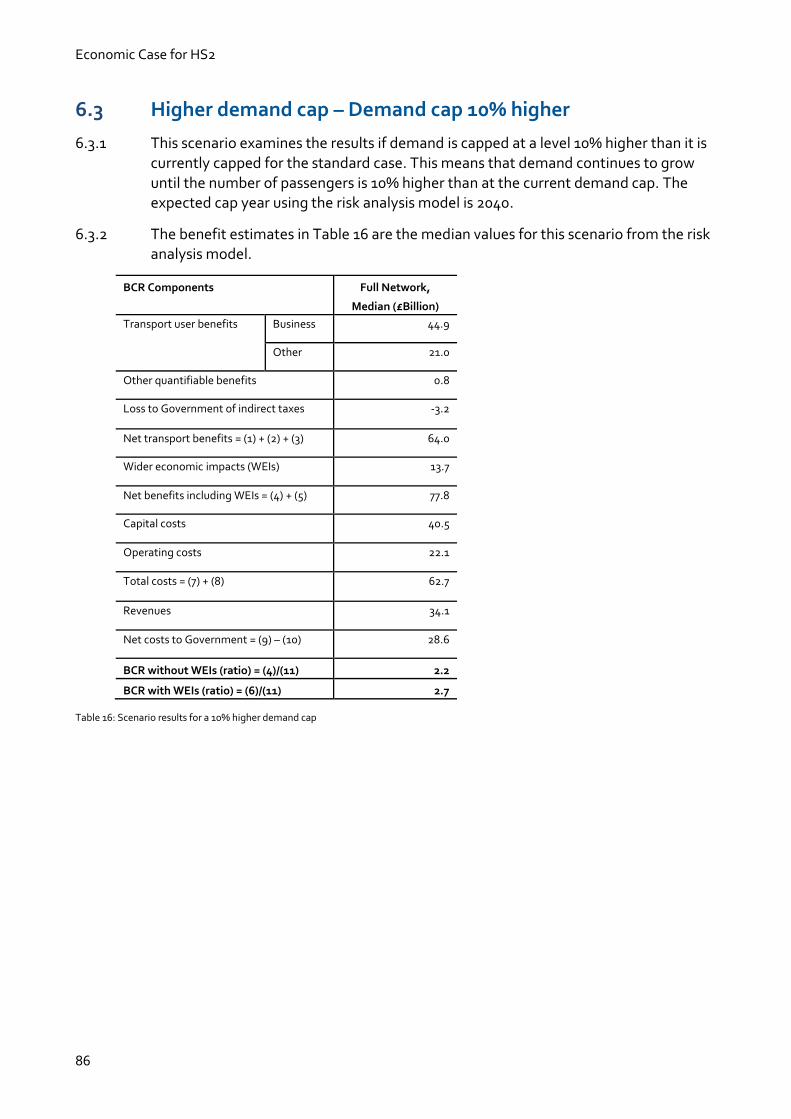
Economic Case for HS2
86
6.3 Higher demand cap – Demand cap 10% higher
6.3.1 This scenario examines the results if demand is capped at a level 10% higher than it is currently capped for the standard case. This means that demand continues to grow until the number of passengers is 10% higher than at the current demand cap. The expected cap year using the risk analysis model is 2040.
6.3.2 The benefit estimates in Table 16 are the median values for this scenario from the risk analysis model.
BCR Components Full Network,
Median (£Billion)
Transport user benefits
Business 44.9
Other 21.0
Other quantifiable benefits 0.8
Loss to Government of indirect taxes -3.2
Net transport benefits = (1) + (2) + (3) 64.0
Wider economic impacts (WEIs) 13.7
Net benefits including WEIs = (4) + (5) 77.8
Capital costs 40.5
Operating costs 22.1
Total costs = (7) + (8) 62.7
Revenues 34.1
Net costs to Government = (9) – (10) 28.6
BCR without WEIs (ratio) = (4)/(11) 2.2
BCR with WEIs (ratio) = (6)/(11) 2.7
Table 16: Scenario results for a 10% higher demand cap

Economic Case for HS2
87
6.4 WebTAG 2012 value of time
6.4.1 The value of times of time and the elasticity of the non-work values with respect to GDP set down in WebTAG have been updated in draft WebTAG 2013 guidance. This scenario demonstrates what the results would show if the previous values of time from WebTAG 2012 were used.
Travel Purpose Old Values of Time
(WebTAG 2012)
New Values of Time
(WebTAG 2013)
Business £47.18 £31.96
Commuting £6.46 £6.81
Leisure £5.71 £6.04
Table 17: Changes in value of time used in WebTAG (2010 prices)
6.4.2 The non-work elasticity in WebTAG 2012 is 0.8, compared to a value of 1.0 in draft WebTAG 2013.
BCR Components Phase One (£billion) Full Network (£billion)
1
Transport user benefits
Business £24.9 £59.6
Other £6.2 £15.3
2 Other quantifiable benefits £0.4 £0.8
3 Loss to Government of indirect taxes -£1.2 -£2.9
4 Net transport benefits = (1) + (2) + (3) £30.3 £72.8
5 Wider economic impacts (WEIs) £5.1 £15.2
6 Net benefits including WEIs = (4) + (5) £35.4 £88.0
7 Capital costs £21.8 £40.5
8 Operating costs £8.2 £22.1
9 Total costs = (7) + (8) £29.9 £62.6
10 Revenues £13.2 £31.1
11 Net costs to Government = (9) – (10) £16.7 £31.5
12 BCR without WEIs (ratio) = (4)/(11) 1.8 2.3
13 BCR with WEIs (ratio) = (6)/(11) 2.1 2.8
Table 18: WebTAG 2012 value of time scenario

Economic Case for HS2
88
6.5 Alternative value of time
6.5.1 As discussed in chapter 6 there is evidence to suggest that the business value of time used to assess high speed rail schemes should be higher and that the non-work values of time should be varied by trip length. This scenario gives results for the ‘alternative value of time’ discussed in chapter 6.
Values used for this test
6.5.2 Value of time figures for all three market segments in our model (business, commuting and leisure) are changed. Different values are derived for each segment and also for long distance and short distance trips in each segment.
6.5.3 In line with the findings from the ITS Leeds report the value applied to benefits from business long distance segment is increased by 40%.
6.5.4 For the long distance leisure and commuting segments we looked at the source data that is used to create the WebTAG values of time. The data from the original survey into commuting and leisure values of time found that the value of time is correlated
with distance. For the purposes of the standard values in WebTAG these values of time by distance are weighted by average trip lengths for commuting and leisure from the NTS, which gives the standard WebTAG figures as a national average for all trips.
6.5.5 Given that HS2 is disproportionately affecting long distance travel, a distance weighted average is unlikely to be appropriate. We have therefore recalculated an average value of time to be used in HS2 appraisal using the proportion of trips by distance from the PLANET model. This is done by calculating the level of benefits by distance and then weighting the original distance segmented values of time according to the distances over which the HS2 benefits are accrued. This weighting was
performed for both phases of HS2 as we expected the average values to be lower for the full network due to the greater levels of inter-regional demand from Birmingham and between locations on the eastern leg. Table 19 shows the values of time derived for the appraisal of long distance benefits.
Business Leisure Commuting
Phase One 44.66 11.11 12.67
Full Network 44.66 10.72 12.31
Table 19: Values of time used to value benefits from the long distance model
6.5.6 This re-weighting leads to significantly higher values for leisure and commuting, almost double the standard values. This is due to the higher values of time seen from the original survey for longer distance travellers.
6.5.7 PFM also contains a set of regional models which is where much of the released capacity benefits occur. We have therefore carried out a similar process for the much shorter trips leisure and commuting trips in these models to prevent any bias. The table below shows the values of time we calculated for commuting and leisure using a similar process to apply to benefits from the regional models. For business trips we used the standard WebTAG values of time.

Economic Case for HS2
89
Business Leisure Commuting
Phase One 31.96 5.27 6.91
Full Network 31.96 5.28 6.91
Table 20: Values of time used to value benefits from PFM regional (short distance) models
6.5.8 Table 21 sets out the point estimate BCR results from this scenario.
BCR Components Phase One (£billion) Full Network (£billion)
1
Transport user benefits
Business £23.2 £55.8
Other £11.9 £30.9
2 Other quantifiable benefits £0.4 £0.8
3 Loss to Government of indirect taxes -£1.2 -£2.9
4 Net transport benefits = (1) + (2) + (3) £34.3 £84.6
5 Wider economic impacts (WEIs) £5.0 £14.8
6 Net benefits including WEIs = (4) + (5) £39.3 £99.4
7 Capital costs £21.8 £40.5
8 Operating costs £8.2 £22.1
9 Total costs = (7) + (8) £29.9 £62.6
10 Revenues £13.2 £31.1
11 Net costs to Government = (9) – (10) £16.7 £31.5
12 BCR without WEIs (ratio) = (4)/(11) 2.1 2.7
13 BCR with WEIs (ratio) = (6)/(11) 2.4 3.2
Table 21: Scenario results for an alternative value of time

Economic Case for HS2
90
6.6 Construction cost target price scenario
6.6.1 In the target cost test the construction cost is assumed to be equal to the target price set for HS2 Ltd.
6.6.2 This test has only been carried out for Phase One because a target price does not yet exist for the Phase Two scheme.
BCR Components Phase One (£billion)
1
Transport user benefits
Business £16.9
Other £7.7
2 Other quantifiable benefits £0.4
3 Loss to Government of indirect taxes -£1.2
4 Net transport benefits = (1) + (2) + (3) £23.8
5 Wider economic impacts (WEIs) £4.3
6 Net benefits including WEIs = (4) + (5) £28.1
7 Capital costs £19.8
8 Operating costs £8.2
9 Total costs = (7) + (8) £28.0
10 Revenues £13.2
11 Net costs to Government = (9) – (10) £14.8
12 BCR without WEIs (ratio) = (4)/(11) 1.6
13 BCR with WEIs (ratio) = (6)/(11) 1.9
Table 22: Economic analysis results for the target price scenario

Economic Case for HS2
91
6.7 The ‘V-network’ 6.7.1 The v-network describes the section of the full network constructed during Phase Two
and excluding Phase One. Table 23 outlines the benefits of Phase Two, given that Phase One is already in operation. The results are calculated using the standard case and subtracting the Phase One results form the full network results. However it is important to understand that to ensure the calculation is logical the analysis period for Phase One must first be extended to 67 years. It is therefore not possible to use only the figures in section 5.2.
6.7.2 The results demonstrate that the sections of the network that are constructed in Phase Two provide a higher value for money than the section constructed under Phase One. However this is only true given the construction of Phase One has already taken place.
BCR Components The V-network
1
Transport user benefits
Business 22.2
Other 11.0
2 Other quantifiable benefits 0.4
3 Loss to Government of indirect taxes -1.7
4 Net transport benefits = (1) + (2) + (3) 31.9
5 Wider economic impacts (WEIs) 8.8
6 Net benefits including WEIs = (4) + (5) 40.7
7 Capital costs 18.7
8 Operating costs 13.7
9 Total costs = (7) + (8) 32.4
10 Revenues 17.3
11 Net costs to Government = (9) – (10) 15.1
12 BCR without WEIs (ratio) = (4)/(11) 2.1
13 BCR with WEIs (ratio) = (6)/(11) 2.7
Table 23: Results for the V-network, Phase Two given Phase One

Economic Case for HS2
92
7 Glossary Definitions Acronym
Appraisal Period - The assumed useful life of the assets for analysis.
Benefit Cost Ratio BCR The ratio of project benefits to project costs
Capital Costs/Capital Expenditure CAPEX The cost of acquiring the physical assets for HS2, including construction,
land purchases and rolling stock.
Cost Benefit Analysis CBA The process of calculating and comparing the benefits and costs of a
project, usually to generate the BCR.
Consumer Price Index CPI A measure of inflation, currently adopted as the government’s official
measure of price increases.
Demand Cap Level - The level of long distance demand at which demand growth is assumed to
halt.
Demand Cap Year - The year in which the demand cap is reached.
‘Do Minimum’ DM The set of train services and demand which are assumed to be in place if
HS2 did not happen – the base case - against which the ‘Do Something’ is
assessed.
‘Do Something’ DS The transport intervention – HS2 scheme - being considered.
Department for Transport DfT The government department responsible for the English (and some of the
Scottish) transport network.
East Coast Mainline ECML The existing rail route connecting London King’s Cross, Peterborough,
Doncaster, Wakefield, Leeds, York, Darlington, Newcastle, Edinburgh and
Aberdeen.
Elasticity - The responsiveness of a change in X as a result of a change in Y
Full Network - The extent of the HS2 network currently being planned for construction.
Gross Domestic Product GDP The market value of all officially recognised final goods and services
produced in the UK within a given period.
Gross Wage Rate - The money you earn based on your hourly pay, before any taxes or other
deductions have been taken out.
Green Book - HM Treasury’s guidance for public sector bodies on how to appraise
proposals before committing funds to a policy, programme or project
High Speed Rail HSR A railway that can operate at speeds of over 150 mph.
Hybrid Bill - A proposal for new legislation that will provide the powers to build HS2.
National Audit Office NAO The body responsible for auditing central government accounts and
reporting on value for money issues.
National Air Passenger Allocation
Model
NAPALM A model used to forecast airport capacity constraints and the distribution
of passengers between airports.
National Rail Travel Survey NRTS A survey of passenger trips on the national rail system in Great Britain on
weekdays outside school holidays.
National Transport Survey NTS The primary source of data on passenger travel patterns in Great Britain.
National Passenger Survey NPS A network-wide survey of customer’ satisfaction with rail travel.
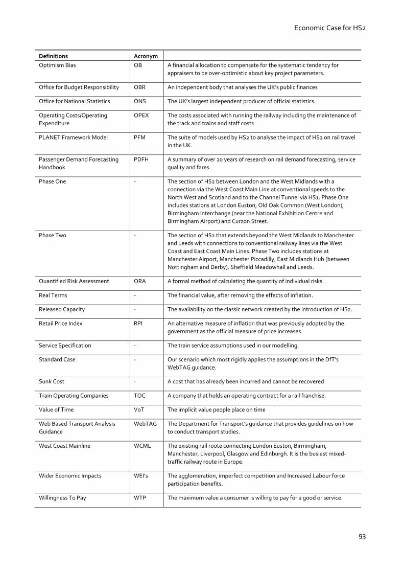
Economic Case for HS2
93
Definitions Acronym
Optimism Bias OB A financial allocation to compensate for the systematic tendency for
appraisers to be over-optimistic about key project parameters.
Office for Budget Responsibility OBR An independent body that analyses the UK’s public finances
Office for National Statistics ONS The UK’s largest independent producer of official statistics.
Operating Costs/Operating
Expenditure
OPEX The costs associated with running the railway including the maintenance of
the track and trains and staff costs
PLANET Framework Model PFM The suite of models used by HS2 to analyse the impact of HS2 on rail travel
in the UK.
Passenger Demand Forecasting
Handbook
PDFH A summary of over 20 years of research on rail demand forecasting, service
quality and fares.
Phase One - The section of HS2 between London and the West Midlands with a
connection via the West Coast Main Line at conventional speeds to the
North West and Scotland and to the Channel Tunnel via HS1. Phase One
includes stations at London Euston, Old Oak Common (West London),
Birmingham Interchange (near the National Exhibition Centre and
Birmingham Airport) and Curzon Street.
Phase Two - The section of HS2 that extends beyond the West Midlands to Manchester
and Leeds with connections to conventional railway lines via the West
Coast and East Coast Main Lines. Phase Two includes stations at
Manchester Airport, Manchester Piccadilly, East Midlands Hub (between
Nottingham and Derby), Sheffield Meadowhall and Leeds.
Quantified Risk Assessment QRA A formal method of calculating the quantity of individual risks.
Real Terms - The financial value, after removing the effects of inflation.
Released Capacity - The availability on the classic network created by the introduction of HS2.
Retail Price Index RPI An alternative measure of inflation that was previously adopted by the
government as the official measure of price increases.
Service Specification - The train service assumptions used in our modelling.
Standard Case - Our scenario which most rigidly applies the assumptions in the DfT’s
WebTAG guidance.
Sunk Cost - A cost that has already been incurred and cannot be recovered
Train Operating Companies TOC A company that holds an operating contract for a rail franchise.
Value of Time VoT The implicit value people place on time
Web Based Transport Analysis
Guidance
WebTAG The Department for Transport’s guidance that provides guidelines on how
to conduct transport studies.
West Coast Mainline WCML The existing rail route connecting London Euston, Birmingham,
Manchester, Liverpool, Glasgow and Edinburgh. It is the busiest mixed-
traffic railway route in Europe.
Wider Economic Impacts WEI’s The agglomeration, imperfect competition and Increased Labour force
participation benefits.
Willingness To Pay WTP The maximum value a consumer is willing to pay for a good or service.