econstorMake Your Publication Visible

A Service of

zbwLeibniz-InformationszentrumWirtschaftLeibniz Information Centrefor Economics

Felbermayr, Gabriel J.; Tarasov, Alexander

Working Paper

Trade and the Spatial Distribution of TransportInfrastructure

CESifo Working Paper, No. 5634

Provided in Cooperation with:Ifo Institute – Leibniz Institute for Economic Research at the University ofMunich

Suggested Citation: Felbermayr, Gabriel J.; Tarasov, Alexander (2015) : Trade and the SpatialDistribution of Transport Infrastructure, CESifo Working Paper, No. 5634

This Version is available at:http://hdl.handle.net/10419/128335

Standard-Nutzungsbedingungen:

Die Dokumente auf EconStor dürfen zu eigenen wissenschaftlichenZwecken und zum Privatgebrauch gespeichert und kopiert werden.

Sie dürfen die Dokumente nicht für öffentliche oder kommerzielleZwecke vervielfältigen, öffentlich ausstellen, öffentlich zugänglichmachen, vertreiben oder anderweitig nutzen.

Sofern die Verfasser die Dokumente unter Open-Content-Lizenzen(insbesondere CC-Lizenzen) zur Verfügung gestellt haben sollten,gelten abweichend von diesen Nutzungsbedingungen die in der dortgenannten Lizenz gewährten Nutzungsrechte.

Terms of use:

Documents in EconStor may be saved and copied for yourpersonal and scholarly purposes.

You are not to copy documents for public or commercialpurposes, to exhibit the documents publicly, to make thempublicly available on the internet, or to distribute or otherwiseuse the documents in public.

If the documents have been made available under an OpenContent Licence (especially Creative Commons Licences), youmay exercise further usage rights as specified in the indicatedlicence.

www.econstor.eu

Trade and the Spatial Distribution of Transport Infrastructure

Gabriel J. Felbermayr Alexander Tarasov

CESIFO WORKING PAPER NO. 5634 CATEGORY 8: TRADE POLICY

NOVEMBER 2015

An electronic version of the paper may be downloaded • from the SSRN website: www.SSRN.com • from the RePEc website: www.RePEc.org

• from the CESifo website: Twww.CESifo-group.org/wp T

ISSN 2364-1428

CESifo Working Paper No. 5634

Trade and the Spatial Distribution of Transport Infrastructure

Abstract The distribution of transport infrastructure across space is the outcome of deliberate government planning that reflects a desire to unlock the welfare gains from regional economic integration. Yet, despite being one of the oldest government activities, the economic forces shaping the endogenous emergence of infrastructure have not been rigorously studied. This paper provides a stylized analytical framework of open economies in which planners decide non-cooperatively on transport infrastructure investments across continuous space. Allowing for intra- and international trade, the resulting equilibrium investment schedule features underinvestment that turns out particularly severe in border regions and that is amplified by the presence of discrete border costs. In European data, the mechanism explains about a fifth of the border effect identified in a conventionally specified gravity regression. The framework sheds light on the welfare costs of second best investment schedules, on the effects of intercontinental trade or of privatized infrastructure provision.

JEL-Codes: F110, R420, R130.

Keywords: economic geography, international trade, infrastructure investment, border effect puzzle.

Gabriel J. Felbermayr

Ifo Institute – Leibniz Institute for Economic Research

at the University of Munich Poschingerstrasse 5

Germany – 81679 Munich felbermayr@ifo.de

Alexander Tarasov National Research University Higher School of Economics

Faculty of Economics Shabolovka 26

Russia – 119049 Moscow atarasov@hse.ru

This version: November 2015 We thank Kristian Behrens, Holger Breinlich, Lorenzo Caliendo, Kerem Cosar, Dalia Marin, Philippe Martin, Pierre Picard, Diego Puga, Esteban Rossi-Hansberg, Philip Ushchev, seminar participants at the universities of Zurich, St. Gallen, Konstanz, Tübingen, Giessen, TU Darmstadt, Linz, Rotterdam, Luxembourg, Ifo Munich, Paris School of Economics, Nottingham, Hohenheim, Milano, and the European University Institute, at the Conference of the Society of Economic Dynamics (SED) in Warshaw, the Congress of the European Economic Association (Toulouse), the European Trade Study Group (Munich), the 17th Conference of the SFB/TR (Munich), the Congress of the German Economic Association (Hamburg), and the workshop “Imperfect Competition and Spatial Economics: Theoretical and Empirical Aspects” (Saint-Petersburg) for valuable comments and discussions. Alexander Tarasov is grateful to the Deutsche Forschungsgemeinschaft through SFB/TR 15 for financial support.

1 Introduction

The provision of transport infrastructure is one of the oldest and most basic government activi-

ties. The roads built by the Inca in South America or by the Romans in Europe bear testimony

to this fact. Indeed, any known civilization has devoted resources to the construction of roads

presumably with the objective to unlock the welfare gains from regional integration.1 On av-

erage, OECD countries spend about 1% of GDP on inland transportation infrastructure and

maintenance. This amounts to about 3% of countries’ public budgets. Emerging or transition

economies spend up to 10% of their budgets on transport infrastructure.2

A large mostly empirical literature demonstrates the important role of infrastructure on

trade costs, trade flows, and welfare. It makes massive efforts to address the suspected endo-

geneity of infrastructure but does not model the processes that determine these costs. So, in

their authoritative handbook chapter, Redding and Turner (2014) ask for “further research ...

examining the political economy of transport infrastructure investments”. The present paper is

a first step towards endogenizing the spatial distribution of transport infrastructure.3

In this paper we focus on land-borne transportation, by far the most important mode for

intracontinental trade in the EU or in North America. Much transport infrastructure spending

is decided decentrally, in particular in the EU, where only about 1% of total spending is at

the Union level and central planning is limited to a small number of projects. For this reason,

we assume that welfare-maximizing national governments allocate infrastructure spending over

space in a non-cooperative fashion. However, while political space is fragmented, consumers

demand goods from all locations in our continuous, linear two-country economy. We show that,

in such a setup, there is inefficiently low global investment in infrastructure. Underinvestment is

particularly severe in border regions. The reason is that national governments do not internalize

the benefits from reductions in domestic transportation costs that accrue to foreign consumers,

and these unaccounted benefits are largest the closer a location is to a national border.

As a consequence, trade across national borders entails higher transportation costs than trade

within countries, holding bilateral distances and market sizes constant. This effect materializes

even in the absence of discrete border costs caused by tariffs or non-tariff measures. However,

the effect is magnified by the existence of such costs. The endogenous emergence of broad border

1A fascinating account of the history of road construction and operation is provided by Lay (1992).2ITF-OECD (2012), p. 4. These investment costs pale in comparison to total social road transport costs

(including time costs and externalities), which have been estimated to amount to 20-25% of GDP (Persson andSong, 2010).

3We formalize the non-cooperative behavior of welfare-maximizing national governments in continuous space.However, we argue that our main results generalize to the median voter model.

2

zones may contribute towards explaining the empirical fact that international borders tend to

restrict international trade much more severely than what observable border costs together with

plausible trade elasticities would suggest (Anderson and van Wincoop, 2003).

We employ data on intra-EU trade flows and transportation costs to calibrate our model

and illustrate our theoretical arguments. We use the setup to simulate a data set of trade flows,

and apply a conventional gravity model. The obtained border effect significantly overestimates

the true border costs; about half of the bias is due to omitting infrastructure; the second half is

a statistical artefact that arises from the high correlation between distance and border. Hence,

endogenous infrastructure investment can explain part of the border effect.

In an intermediate step of our theoretical analysis, we propose a useful mapping between

the spatial distribution of infrastructure spending within an interval into transportation costs

between the two endpoints of this interval. This mapping is consistent with the concave rela-

tionship between geographical distance and transport costs documented in the data. The link

between infrastructure investment over space and transportation costs is shaped by the elasticity

of substitution between investment at different locations. We embed this structure into a simple

model of intra- and international trade, where each location produces a unique differentiated

product which is subject to transportation costs.

We find that the optimal infrastructure investment at some point in space is not only deter-

mined by local conditions at that point, but also – and predominantly – by the situation in other

locations that produce and demand goods which transit through that point. The enlargement

of a country – e.g., the reunification of Germany – leads to a reallocation of investment away

from formerly central regions towards the former border. A higher degree of substitutability be-

tween investments at different addresses has an ambiguous effect on investment while a higher

elasticity of substitution between goods produced at different location reduces investment.

Using real data on EU trade flows, we provide econometric support for the role of transport

infrastructure in shaping the border effect. Employing road distance or, even better, travel time,

as proxies for transportation costs instead of great-circle distance, the estimated trade-inhibiting

effect of the border falls by about a quarter. We provide various sensitivity checks to make sure

that our empirical result is not driven by reverse causation.

We extend our analysis by adding a non-contiguous country which supplies and demands

goods to and from our two-country continent. We find that an increase in the economic mass

of this overseas trading partner induces a reallocation of spending towards coastal regions and

away from the hinterland, strengthening the border effect.

Our main result is robust to a number of model variations. First, we discuss how privately

3

operated toll roads would change our results. Second, we study a special case where governments

outsource the design and operation of roads to domestic private monopolists but regulate the

fee system. These firms care only about profits and not about welfare. However, the central

issue leading to inefficient investment variation persists: the monopolists underinvest more in

locations close to the border where the positive externality on foreign infrastructure operators

is largest. Third, we argue that allowing for labor mobility does not undo underinvestment at

the border relative to first best. However, whether the non-cooperative equilibrium features a

bimodal investment pattern depends on the size of discrete border costs. Fourth, we demonstrate

that our central planner results are similar to the outcome expected from a median voter model.

Our paper is related to at least four important strands of literature. First, it connects

with papers that study the importance of geographical frictions and transportation costs for

trade and welfare. Typically, the literature has treated those costs as exogenous. Limao and

Venables (2001) find that up to 60 percent of the cross-country variation in transport costs

is due to transport infrastructure and that high cost of land-borne transportation is a more

relevant trade barrier than the costs of maritime transportation. Venables (2005) argues that

infrastructure explains a larger share of spatial income inequality than sheer geography. Many

existing papers assume that countries (or regions) do not have a geographical extension. Recent

work provides more spatial detail, but continues to treat infrastructure as exogenous. Cosar and

Demir (2014) show that the upgrading of motorways in Turkey significantly increases exports of

transport-intensive goods of landlocked cities. Allen and Arkolakis (2014) incorporate realistic

topographical features into a spatial model of trade. They find that the introduction of the US

interstate highway system has reduced the costs of a coast-to-coast shipment by about a third.

Duranton et al. (2014) use data on US interstate highways to show that highways within cities

cause them to specialize in sectors that have high weight to value ratios. Using a multi-region

general equilibrium model of trade, Donaldson (2014) and Donaldson and Hornbeck (2015)

analyze the welfare gains from railroads in India and the United States, respectively. They find

that improved market access through reduced transport costs creates trade and generates welfare

gains, but that it also leads to trade diversion. Behar and Venables (2011) and Redding and

Turner (2014) provide excellent surveys. While they cite empirical work on the determinants of

transportation costs, they do not provide theoretical references on their endogenous emergence.

Second, our paper is related to a small literature that endogenizes transportation costs,

usually by introducing a proper transportation sector. Using an economic geography model,

Behrens and Picard (2011) show that the prices for transporting differentiated goods increase in

the degree of spatial specialization of the economy and that this channel dampens core-periphery

4

patterns. While their model has a competitive transport sector, Hummels et al. (2009) provides

evidence that monopolistic market structure in the transport sector restricts trade. These papers

do not analyze the endogenous emergence of road infrastructure.

Third, our paper is related to literature that jointly considers international and intranational

aspects of trade. Courant and Deardorff (1992) emphasize the importance of trade within

countries for trade patterns across countries. Rossi-Hansberg (2005) studies the effects of small

border costs on the regional distribution of workers within a country and assesses the implications

of the equilibrium population distribution on intra- versus international trade flows. However,

his focus is not on infrastructure investment.

Fourth, our paper relates to work on the border puzzle. Transport costs are usually related

to geographical distance while the border effect is attributed to some lumpy cost that material-

izes when crossing a border. Anderson and van Wincoop (2003) estimate that the US-Canadian

border reduces international trade relative to intranational trade by a factor of 4.7.4 Explana-

tions for fixed border costs abound. Among other things, they are related to informational costs

(Casella and Rauch, 2003), networks (Combes et al., 2005), or exchange rates (Rose and van

Wincoop, 2001). Border effects exist also within countries, where the above explanations do not

help.5 Our setup shows that border effects can arise even in the absence of explicit costs at the

border.

The structure of the paper is as follows. Section 2 presents some stylized facts on the

transportation sector that inform our modeling choices. Section 3 explains our formulation of

the mapping between the spatial distribution of infrastructure investment and transport costs.

Section 4 sets up the general equilibrium environment which motivates intra- and international

trade and analyzes the optimal infrastructure investment schedule in a closed economy. Section

5 moves to a setting of two symmetric open economies and derives our core results on the

endogenous emergence of border regions. Section 6 provides empirical evidence supporting our

analysis while Section 7 discusses several extensions. Section 8 concludes.

4Prior to Anderson and van Wincoop (2003), McCallum (1995) compares trade flows within Canada to flowsbetween Canadian provinces and U.S. states, controlling for distance and regional GDPs. Everything else equal,crossing the border reduces trade by a factor as high as 22. For Europe, Nitsch (2000) finds that on averageintranational trade is about 10 times higher than international one. Nitsch arrives at his results after controllingfor cultural proximity (language), along other conventional gravity covariates. Wei (1996) constructs measures forimports of countries to themselves and compares this with imports from a statistically identical foreign country.He finds that the former magnitude is 2.5 times larger than the latter. Helliwell (1998) offers a comprehensiveoverview of the pre Anderson and van Wincoop state of the econometric literature.

5Okubo (2004) shows a border effect for trade between Japanese regions, Wolf (2000) for the US, and Combeset al. (2005) for their sample of French departments.

5

2 Stylized facts

Here, we present some stylized facts on transportation costs and transport infrastructure.

Fact 1: Transport costs vary across space. Direct data on transportation costs is scarce.

Representative marginal costs for freight transportation amount to 1.54 Euro per kilometer on

average around 2008 in the United Kingdom. Fuel (including taxes) and travel time account

for 44% and 38% of the total, respectively (Braconier et al., 2013). Combes and Lafourcade

(2005) provide generalized transportation cost data for a sample of 8742 French city pairs in

1993. Average road transportation costs are 5.16 French Francs per kilometer.6 The data

also reveals a strong degree of variation in bilateral transportation costs: transportation costs

at the 5% percentile are 4.54 while at the 95% percentile they are 5.86 per kilometer. The

standard deviation is 0.43. Looking at the average per kilometer cost of transiting one of the

94 French departments,7 one discovers an even higher standard deviation of 1.12. Only part of

this variation is explained by variables such as economic activity, density, or topography.8

Fact 2: Transport costs are non-convex in distance. Usually, in economic geography

models (Fujita et al., 1999), transportation costs are modeled as exponential functions of dis-

tance.9 However, the data reject convexity. Figure 1 provides an illustration based on data

by Combes and Lafourcade (2005). Regressing the log of transportation costs between capitals

of French departements on the log of geographical distance reveals an elasticity of 0.90 with a

standard error of 0.02. The hypothesis of the elasticity being equal to unity is rejected at the

1% level.10

Fact 3: Infrastructure investment and transportation costs are closely related. A

large empirical literature, already discussed in the introduction, establishes a close link between

infrastructure investment, transportation costs, and the benefits of economic integration; see

6Assuming an inflation rate of 3% a year and applying the FF/Euro conversion rate of 6.55957, this wouldamount to about 1.25 Euro in 2008 current prices.

7To obtain a measure of transit costs, we average total variable transport costs per kilometer between neigh-boring departements, using the neighbors’ area as weights.

8In Appendix B (Table 8), we relate average transit costs to GDP, area and population of the respectivedepartment, the ruggedness of territory, and to geographical remoteness. We find that average transportationcosts are higher in geologically difficult, less densely populated and poorer departments. Everything else equal,they are also higher in less central regions. Geography explains about 16% of transport cost variation; addingGDP, area and population drives the explanatory power of the model up to 58%. Hence, such a ‘naive’ modelleaves about 40% of variance unexplained.

9See McCann (2005) for criticism.10Using robust regression methods to punish outliers leads to an elasticity of 0.92, still different from 1.00 at

the 1% level. The same holds true if one restricts the sample to distances below 200, 150 or 100 km.

6

Figure 1: Transportation costs and distance: a concave relationship

050

010

0015

00ge

nera

lized

tran

spor

tatio

n co

sts,

in F

F

0 100 200 300distance in km

Notes. Generalized transportation costs between capitals of French departements in French Francs (1993) as afunction of geographical distance in km.

Limao and Venables (2001) on cross-country evidence, Allen and Arkolakis (2014) or Duranton

et al. (2014) on US interstate highways, Donaldson (2014) and Donaldson and Hornbeck (2015)

on railroads in India and the US, respectively, or Cosar and Demir (2015) on roads in Turkey.

Fact 4: Intracontinental trade flows are mostly land-borne. Table 1 reports data for

merchandise trade within NAFTA and Europe. In 2010, between 72 and 75% of the value of

total regional trade is transported on roads or railways. Measured by tonnage, the shares are

lower as much bulk transportation is water-borne. While the importance of air-borne traffic is

increasing, it still is almost irrelevant in intracontinental trade.

Fact 5: Transport infrastructure is publicly provided. Infrastructure and maintenance

spending on roads amounts to about 1% of GDP across OECD countries (average across 2001-

2009).11 Countries with difficult territory (such as Japan, Switzerland or Italy) have higher than

average spending. Almost all spending on roads and railways is financed by governments, even

if private public partnership agreements are becoming increasingly popular.

Fact 6: Regional governments influence interregional infrastructure projects sub-

stantially. Within countries, there is a substantial amount of centralization of infrastructure

11OECD Economic Outlook 91 database. There is some disagreement about measurement; the CongressionalBudget Office puts total public spending for transportation and water infrastructure between 1.2% and 1.5% ofGDP in the 1956-2007 period.

7

Table 1: Intercontinental merchandise trade by transport mode: NAFTA and EU

North America French intra-EU tradevalue weight value weight

bn. USD % mio. tons % bn. EUR % mio. tons %

Truck 557 61 187 29 338 69 200 59Rail 131 14 134 21 15 3 15 4Air 45 5 1 0 22 4 0 0Water 81 9 210 32 70 14 77 23Pipeline 63 7 106 16 n.a. n.a. n.a. n.a.Other 40 4 9 1 45 9 45 13

Total 918 100 646 100 491 100 336 100

Notes: Data refer to 2010 (except French quantity information: 2006). Sources:

US department of transportation, Freight Facts and Figures 2011, Table 2.8.,

www.ops.fhwa.dot.gov\freight\freight analysis\nat freight stats\docs\11factsfigures\index.htm

and Commissariat du development durable, www.statistiques.developpement-

durable.gouv.fr\transports\873.html.

planning and spending. Nonetheless, local governments matter, too. In the US, about 90% of

all spending on infrastructure and equipment falls on the local or state level, but federal trans-

fers have become quite important over time (Congressional Budget Office, 2010). In Europe,

member states decide almost exclusively on their own about transport infrastructure investment

projects. There is some coordination at the Union level through the so called Trans-European

Transport Network, but the budget has been limited to about 1 billion Euro per year over the

2007-2013 spending period. This is less than 1% of overall spending on infrastructure in the EU

(120 billion Euro).12

Fact 7: Distance elasticities and border effects in gravity models. A voluminous

empirical literature finds that geographical distance restricts trade flows; see Head and Mayer

(2014). In their meta analysis across appropriately specified gravity models, the authors find a

median elasticity of trade flows with respect to great circle distance of about -1.1 and a median

border effect (i.e., the trade inhibiting effect of a border as compared to trade within a country)

of -1.6. In our empirical application using very recent European data, the distance elasticity is

also -1.1, but the border effect is -0.8.13

12http://ec.europa.eu/transport/infrastructure/tentec/tentec-portal/site/en/abouttent.htm. In the period2014-2020, centralized spending rises about threefold. However, this still keeps decentralized spending at about97% of total spending.

13We describe the data, methodology and results in Section 6 but mention our findings here, because they willinform the numerical illustrations of our theory.

8

3 Modeling transportation costs

Models of international trade and economic geography typically employ Samuelson’s (1952)

iceberg trade costs assumption: in order to receive one unit of the good at some location x,

T (x, z) ≥ 1 units of that good have to leave the factory at location z.14 A share 1− T (x, z)−1

of the good ‘melts’ in transport; the share T (x, z)−1 arrives at x when one unit of the good

is shipped at z. This formulation represents a dramatic simplification (McCann, 2005). But

it has proved convenient, because it makes the introduction of a specific transportation sector

redundant.

In this paper, we stick to the iceberg formulation, but we let transportation costs between

two addresses x and z depend on cumulative infrastructure investment. Public infrastructure

investment refers to the process of investing some resource at specific locations s with the aim

of reducing transportation costs.15 We assume that the set of geographic locations, S, is given

by an interval, [0, s], where s characterizes the geographical size of the economy. In contrast

to a circular economy, the linear specification appears preferable since it features a natural

periphery.16

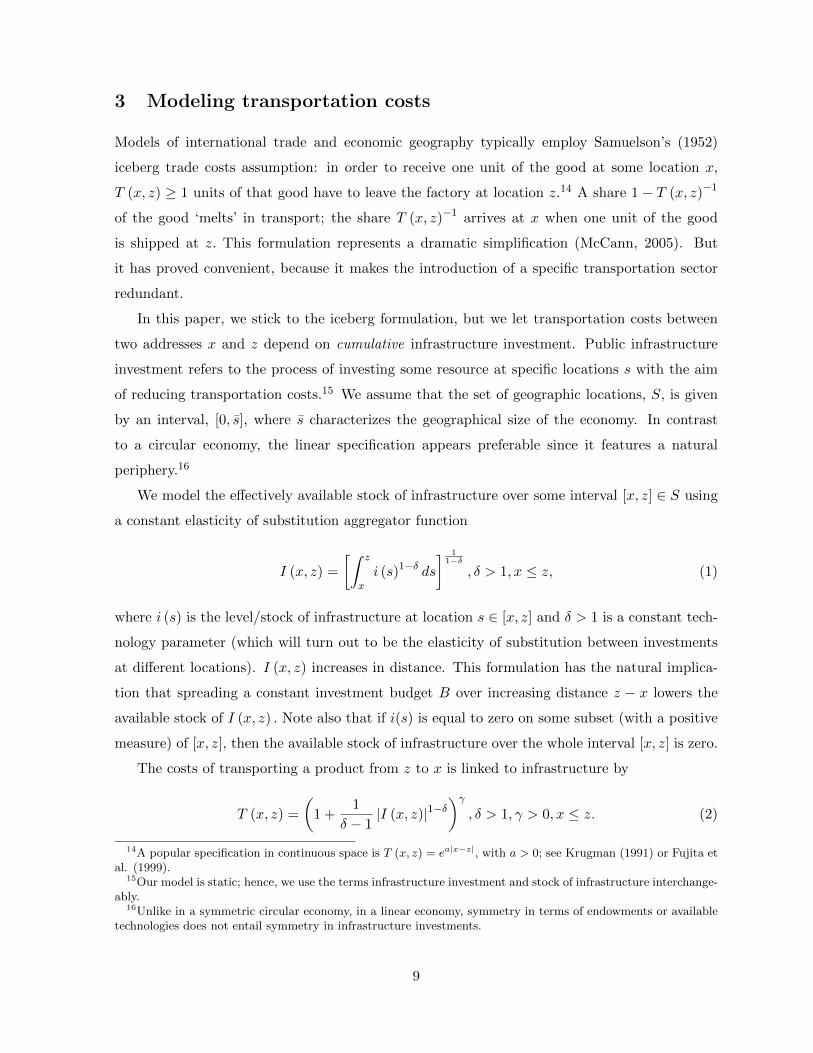
We model the effectively available stock of infrastructure over some interval [x, z] ∈ S using

a constant elasticity of substitution aggregator function

I (x, z) =

[∫ z

xi (s)1−δ ds

] 11−δ

, δ > 1, x ≤ z, (1)

where i (s) is the level/stock of infrastructure at location s ∈ [x, z] and δ > 1 is a constant tech-

nology parameter (which will turn out to be the elasticity of substitution between investments

at different locations). I (x, z) increases in distance. This formulation has the natural implica-

tion that spreading a constant investment budget B over increasing distance z − x lowers the

available stock of I (x, z) . Note also that if i(s) is equal to zero on some subset (with a positive

measure) of [x, z], then the available stock of infrastructure over the whole interval [x, z] is zero.

The costs of transporting a product from z to x is linked to infrastructure by

T (x, z) =

(1 +

1

δ − 1|I (x, z)|1−δ

)γ, δ > 1, γ > 0, x ≤ z. (2)

14A popular specification in continuous space is T (x, z) = ea|x−z|, with a > 0; see Krugman (1991) or Fujita etal. (1999).

15Our model is static; hence, we use the terms infrastructure investment and stock of infrastructure interchange-ably.

16Unlike in a symmetric circular economy, in a linear economy, symmetry in terms of endowments or availabletechnologies does not entail symmetry in infrastructure investments.

9

Transportation costs are symmetric in the sense that delivering a product from x to z costs the

same as delivering a product from z to x. The parameter γ governs the effect of the total stock

of infrastructure on transportation costs.

The choice of functional forms (1) and (2) proves convenient, as will become transparent

below. Moreover, the formulation has properties long discussed (but rarely formally modelled

in a general equilibrium context) by transport economists (Winston, 1985, or Gramlich, 1994).

Lemma 1 Generalized iceberg trade costs T (x, z) have the following properties:

(i) T (x, z) ≥ 1 with T (x, x) = 1 and T (x, y)T (y, z) ≥ T (x, z).

(ii) T (x, z) = (1 + a|z − x|)γ , if i (s) is a constant ı over the interval [x, z], and a = ı1−δ/ (δ − 1).

(iii) T (x, z) =∞, if i (s) = 0 on some subset (with a positive measure) of [x, z].

(iv) T (x, z) is increasing in distance: i.e. for fixed x a more distant location z results in higher

transportation costs. Moreover, if i(s) is a differentiable function on S, T (x, z) is concave

in distance if the distance-induced increment to the trade cost gradient is outweighed by

an improvement in infrastructure. That is, if (γ − 1) [a (z)]2 / (T (x, z))1/γ < i′ (z) i (z)−δ

where a (z) = i (z)1−δ / (δ − 1).

(v) The (interregional) elasticity of substitution between infrastructure investment at different

locations is 0 < 1/δ < 1, so that investments at different locations are gross complements.

(vi) Investment smoothing property: if investment costs do not vary across locations, then the

cost-efficient way to achieve some exogenous target level of transportation costs involves a

flat spatial investment profile

i (s) =

(z − x) /[(δ − 1)

(T 1/γ − 1

)]1/(δ−1).

where T > 1 is the target level of iceberg transportation costs.

Proof The first three properties directly follow from the definition of the trade costs in

(2). The last three properties are proved in Appendix A.

Property (i) establishes that, for any x, y, and z, the triangle inequality holds: T (x, y)T (y, z) ≥

T (x, z) (the strict inequality holds, if x, y, and z represent different locations). So, it is cheaper

to transport products directly to a destination address, rather than through some intermediate

address.

10

Property (ii) shows that equation (2) collapses to the specification almost exclusively used in

empirical gravity models (with a = 1); see Head and Mayer (2014). Our specification also allows

for concavity of transportation costs with respect to distance documented in the data. Iceberg

transportation costs are concave in distance, as long as the component of dT (x, z) /dz driven by

variation in infrastructure investment outweighs the pure distance component of dT (x, z) /dz

(see property (iv) in the above lemma). Hence, in general, whether T (x, z) is concave in distance

depends on the spatial allocation of infrastructure investment and the values of γ and δ.

Properties (v) and (vi) exploit an isomorphism between (2) and the usual representation of

utility in an optimal growth model. The parameter δ measures the ease with which infrastructure

investment at some address can substitute for investment at another place. The restriction δ > 1

ensures that investments at different places are gross complements: investment at some address

makes investment at some other place more worthwhile, which seems realistic and is consistent

with the data.17

4 Infrastructure investment and intraregional trade

In a first step, we incorporate our modeling of transportation costs and infrastructure into a

simple model of intranational trade. Later we introduce international trade.

4.1 Geographical space and goods space

We assume that, at each location s ∈ S, there is a representative household who inelastically

supplies m (s) > 0 units of labor. The total endowment of labor in the economy is then equal

to∫s∈Sm(s)ds, which we define as L.

Each location produces both a homogeneous agricultural and a spatially differentiated indus-

trial good. Consumers consume both goods and perceive industrial goods produced at specific

locations as imperfect substitutes. There are no costs of transporting the agricultural good.

Moreover, the agricultural good serves as an input into infrastructure provision.18 Each lo-

17We do not allow for incremental transport costs incurred at address s to depend on the volume of traffictransiting through s. Actually, in equilibrium, the contrary will hold: more traffic at s will encourage the plannerto invest more in infrastructure, thereby driving down the gradient of T. This lowers the incremental trade costsat s for all units of goods that transit through s.

18The assumption of a freely tradable agricultural good which is produced at every location is frequently used inmodels of economic geography. It provides tractability as wages are equalized across space (in nominal terms). Analternative/equivalent way to model infrastructure provision is to assume that the only input into infrastructureis labor, which in turn is perfectly mobile between locations (within an economy). But consumption takes place atthe place of origin. This will equalize wages across locations (which is in the present model done by the presenceof the homogenous agricultural good) making the presence of the agricultural good redundant.

11

cation s is home of consumers and producers. We denote addresses of consumers by x and

addresses of producers by z.

We assume that locations may differ with respect to topological circumstances. Specifical-

ly, infrastructure at address s is produced according to a linear production function i (s) =

b (s) /q (s), where b (s) denotes the input of the agricultural good used for infrastructure invest-

ment, and 1/q (s) > 0 measures the rate at which that resource is transformed into infrastructure.

We restrict q (s) to be continuously differentiable. Feasibility of an investment policy i (s) re-

quires∫s∈S q (s) i (s) ≤ B, where B is the amount of agricultural good invested in infrastructure

and will be endogenously determined by government policy.

4.2 Consumption

The utility function of a representative household at location x is a monotone transformation of a

Cobb-Douglas aggregate over the homogeneous agricultural good and a Dixit-Stiglitz aggregate

over industrial goods:

U (x) =[cA (x)

] αρ(1−α)(1−ρ)

(∫z∈S

cI (x, z)ρ dz

) 11−ρ

, (3)

with α ∈ (0, 1) , 0 < ρ < 1, where cA (x) denotes the total quantity of the agricultural good

consumed at address x and cI (x, z) is the quantity of an industrial variety produced at address

z and consumed at x.19

Let Y n (x) denote household x′s net income in terms of a numeraire to be defined below.

Then, the budget constraint of household x is Y n (x) = cA (x) pA (x) +∫z∈S c

I (x, z) pI (x, z) dz,

where pA (x) is the price of the agricultural good at location x and pI (x, z) is the price of a

variety imported from location z and consumed at x.

The utility maximization problem implies that the demand functions for the agricultural

good and a certain variety of the industrial good are respectively

cA (x) =αY n (x)

pA (x)and cI (x, z) = (1− α)Y n (x)

pI (x, z)−σ

P I (x)1−σ , (4)

where σ ≡ 1/ (1− ρ) and

P I (x) =

[∫z∈S

pI (x, z)1−σ dz

] 11−σ

(5)

19Notice that U(x) is a positive monotonic transformation U(x) = [U(x)]ρ/((1−α)(1−ρ)) of the usual Cobb-

Douglas formulation U(x) =[cA (x)

]α [uI (x)

]1−α. The transformation makes the theoretical analysis of the

model more tractable (without qualitatively changing the main conclusions).

12

is the price index for industrial goods at location x.

The indirect utility attainable at prices pA (x), pI (x, z) and income Y n (x) can be written

as

V (x) = A[pA (x)

]−αρ/((1−α)(1−ρ)) [P I (x)

]1−σ(Y n (x))ρ/((1−α)(1−ρ)) , (6)

where A ≡(αα/(1−α) (1− α)

)ρ/(1−ρ).

4.3 Production

At each location z ∈ S, the agricultural and the industrial good are produced under conditions

of perfect competition. The only input of production is labor. Production functions for the

two types of goods are linear yA(z) = blA(z) and yI(z) = lI(z), where b > 0 is a productivity

parameter common to all locations. Output quantities are denoted by yA (z) and yI (z), and

labor inputs by lA (z) and lI (z) , respectively.

We assume that, within addresses, workers are perfectly mobile across agricultural and in-

dustrial firms. This in turn implies that pA (z) = w (z) /b and pI (z) = w (z), where w (z) is the

wage rate (expressed in units of numeraire) at address z. Industrial goods bear transportation

costs. We assume that there are no trade costs other than transportation costs.20 Hence, the

c.i.f. prices faced by consumers differ from the f.o.b. (ex-factory) prices. In particular, a house-

hold at x faces the price pI (x, z) = pI (z)T (x, z) for a variety of the industrial good imported

from location z. In contrast, the agricultural good can be transported freely.

4.4 Equilibrium

In this paper, we impose a non-full-specialization (NFS) assumption: there is always a strictly

positive quantity of agricultural production at each location. The NFS assumption introduces

factor price equalization in terms of the agricultural good.21 We may therefore choose the

agricultural good as the numeraire and set pA (z) = 1 for all z ∈ S. Since pA (z) = 1 for any z,

we drop the superscripts A and I in the following.

As the price of the agricultural good is normalized to unity, the wage rate at location z, w(z),

is equal to b. The gross income at location x in terms of the numeraire is then Y (x) = bm (x).

Finally, from our assumption on technology, the c.i.f. prices of industrial goods are p (x, z) =

bT (x, z) .

20In Section 5, when we consider international trade, we will introduce a discrete trade friction at the border.21Relaxing the NFS assumption would allow to study the interaction between infrastructure investment policies

and regional specialization patterns. This is an interesting issue that raises additional complications. It is thereforeleft to future research.

13

The government imposes a lump-sum tax with rate t, which is assumed identical across

addresses s ∈ S. Thus, the net income at location x, Y n (x), is (1− t)bm (x). Total tax income

is

B = bt

∫s∈Sc

m (s) ds = btL.

Substituting the expressions for net household income and for the price index, we can now

rewrite the indirect utility function in (6) as

V (x) = Ω(1− t)(σ−1)/(1−α)m (x)

[∫z∈S

T (x, z)1−σ dz

], (7)

where m (x) = m (x)(σ−1)/(1−α) and Ω ≡(αα/(1−α) (1− α) bα/(1−α)

)ρ/(1−ρ)is a constant.

4.5 The choice of infrastructure investment

In this section, we characterize optimal policies ia(s), tas∈S in a closed economy. The social

planner chooses the infrastructure investment and the tax rate to maximize total welfare – the

sum of individual utilities – in the economy. Ignoring the irrelevant constant, we have

ia (x) , tax∈S = arg max

(1− t)

(∫x∈S

m (x) v(x)dx

) 1−ασ−1

∣∣∣∣∫x∈S

q (x) i (x) dx ≤ btL

, (8)

where

v(x) =

∫z∈S

T (x, z)1−σ dz. (9)

A sufficient condition for concavity of the objective function in (8) is

1 + (γ (δ − 1))−1 > σ > 2− α. (10)

The first inequality means that T (x, z)1−σ is concave with respect to infrastructure investments,

implying that the consumption utility, v(x), is concave in infrastructure investments as well.22

The second inequality, which would be always met if σ ≥ 2, implies that the objective function

is concave in v(x). As a result, the objective function is concave with respect to infrastructure

investments.23

Next, we characterize the solution of the planner’s problem. Note that, without loss of

22The function(

1 + 1δ−1

x1−δ)γ(1−σ)

is strictly concave on [0,∞) if and only if γ(σ − 1) (δ − 1) < 1. In turn,

T (x, z)1−σ is concave with respect to infrastructure investment.23Our results are qualitatively robust to changes in the functional form of the transportation costs as long as

T (x, z)1−σ is concave in i (s), s ∈ [x, z], and has an unbounded derivative at i(s) = 0.

14

generality, we find the solution among continuous functions on [0, s]. That is, social welfare is

maximized with respect to ia (x), where ia (x) is continuous.

Proposition 1 The optimal allocation of infrastructure spending across space and the opti-

mal tax rate chosen by a social planner under autarky are implicitly determined by the following

system of equations:

ia (x)δ =bγ (1− α) (1− ta)L

q(x)

[φL(x) + φR(x)

], (11)

ta =

∫s∈S q (s) ia (s) ds

bL, (12)

where φL (x) and φR (x) denote aggregate marginal utilities from investing to the left or the right

of x, respectively, and are defined as

φL(x) =

∫ x0 m (s)

[∫ sx

(1 + 1

δ−1

∫ ts i

a (r)1−δ dr)γ(1−σ)−1

dt

]ds∫

s∈S m (s) v(s)ds,

φR(x) =

∫ sx m (s)

[∫ x0

(1 + 1

δ−1

∫ st i

a (r)1−δ dr)γ(1−σ)−1

dt

]ds∫

s∈S m (s) v(s)ds.

Proof In the Appendix.

The investment at location x is higher, the larger the sum φL (x)+φR (x) or the lower the cost

of infrastructure at the location, q(x). In the next proposition, we summarize some additional

properties of the optimal infrastructure investment function, ia (x), and the consumption utility,

v(x).

Proposition 2 The optimal infrastructure investment function, ia (x), and the consumption

utility, v(x), have the following properties:

(i) The infrastructure investments are zero at the borders of the region: ia (s) = ia (0).

(ii) If q(x) is continuously differentiable, ia (x) is increasing in the neighborhood of zero and

decreasing in the neighborhood of one: specifically, (ia (x))′x=0 =∞ and (ia (x))′x=s = −∞.

(iii) If there is no variation in the cost of infrastructure investment and the household size

across the locations: q(x) = q and m(x) = m for any x ∈ S, then v(x) and ia (x) are

symmetric around x = s/2 and have a hump shape with maximum at x = s/2.

15

Proof The first property immediately follows from the definitions of φL(x) and φR(x).

Specifically, we have that φL(s) = φL(0) = φR(s) = φR(0) = 0. The last two properties are

established in the Appendix.

According to the proposition, if there is no variation in the cost of infrastructure and in

household size, the optimal infrastructure is symmetric around the middle point of the [0, s]-

interval. So, transportation costs in central parts of the country are lower than in peripheral

parts and, thereby, households located closer to the middle point have higher indirect utility.

The intuition is that, at the optimum, the sum of marginal benefits from investment needs to

be equalized to the constant cost of investment at each location and this is achieved by higher

investment in central locations.

4.6 Comparative statics

The optimal infrastructure investment at location x is implicitly determined by

ia (x) =

(γ (1− α)

(bL−

∫s∈S q (s) ia (s) ds

)q(x)

(φL(x) + φR(x)

))1/δ

(13)

≡ ia (x, Ia, ε) ,

where Ia represents the infrastructure profile in the economy and ε is the set of parameters in

the model. Thus, changes in ia(x) due to changes in ε are implicitly determined by

∂ia (x)

∂ε=∂ia (x, Ia, ε)

∂ε+∂ia (x, Ia, ε)

∂Ia∂Ia

∂ε. (14)

The first term in the right-hand side of (14) captures the direct effect of ε on ia (x), while the

second term stands for the indirect effects.

Proposition 3 Changes in the parameters in the model have the following effects on the

optimal infrastructure profile in a closed economy:.

(i) A rise in b increases ia(x) for all x.

(ii) Assuming that m(x) = m for all x, a rise in m increases ia(x) for all x.

(iii) Assuming that q(x) = q for all x, a rise in q decreases ia(x) for all x.

(iv) Assuming that m(x) = m for all x, a rise in s has a positive direct effect on ia(x) for

x close to the right border and has an ambiguous impact on the investments at the other

16

Figure 2: Closed economy equilibrium investment loci: comparative statics

(a) Moving s from 500 to 700 (b) Moving γ from 0.86 to 0.7

0 100 200 300 400 500 600 7000

20

40

60

80

100

120

140

160

180

0 50 100 150 200 250 300 350 400 450 5000

20

40

60

80

100

120

140

160

180

(c) Moving σ from 2.7 to 2.0 (d) Moving δ from 1.65 to 1.5

0 50 100 150 200 250 300 350 400 450 5000

50

100

150

200

250

0 50 100 150 200 250 300 350 400 450 5000

20

40

60

80

100

120

140

160

180

Notes. Solid black curve: default investment distribution with σ = 2.7, δ = 1.65, γ = 0.86, α = 0.5, q(x) =q = 1, m(x) = m = 1000, b = 1, and s = 500. Dashed red curves: distributions resulting from alternativeparameterizations. See Table 2 for calibration details.

locations. If in addition q(x) = q for all x, then a rise in s has a positive direct effect on

ia(x) for all x ∈ S.

Proof In the Appendix.

While parts (i) to (iii) of Proposition 3 account for direct and indirect effects, part (iv)

describes only the direct effect of an increase in s (which, holding population density constant,

amounts to an enlargement of a country, such as the reunification of Germany in 1990). Figure

2(a) provides a numerical illustration of the overall effect of a rise in s on the infrastructure

profile.24 Enlargement of a country diverts investment away from locations sufficiently far from

the added territory. This is consistent with the German post-reunification experience.25

24In the figure we consider a discrete variation of the model that has similar properties as the continuous model(see more on the choice of the parameterization in Section 5.3).

25See the information onwww.bmvi.de/SharedDocs/DE/Artikel/StB/entwicklung-der-autobahnen-in-deutschland-seit-der-wiedervereinigung.html.

17

The formal analysis of the comparative statics with respect to γ, δ, and σ is not tractable;

so, we turn to numerical experiments. A lower value of γ makes the dependence of trans-

portation costs on infrastructure investments weaker. Therefore, the returns from investing in

infrastructure at all locations are smaller, leading to lower ia (x) at all locations (Figure 2(b)).

Lower σ makes the varieties of the differentiated product less substitutable, increasing the ben-

efits of intra- and international trade. As a result, incentives to invest in infrastructure go up

and, therefore, ia(x) rises ((Figure 2(c)). In contrast, changing δ has an ambiguous impact on

infrastructure investment. With the chosen parameterization, a decrease in δ from 1.65 to 1.5

makes investments at different locations more easily substitutable. This decreases infrastructure

investments at all locations and also lowers the spatial variance of investment (Figure 2(d)).

5 Infrastructure investment and international trade

Now, we assume that the world economy consists of two independent countries, each with its

own government that decides on infrastructure investment in a non-cooperative way. However,

consumers demand goods from all over the world. Thus, we have a situation with ‘globalized

markets, but regional politics’. Otherwise, we maintain all earlier assumptions. To start with,

we assume that countries are symmetric. In particular, the world geography is described by the

[0, 2s]-interval, where locations from [0, s] and (s, 2s] represent the home and the foreign country,

respectively. To isolate a pure border effect on the equilibrium infrastructure profile we assume

away any variation in the costs of infrastructure and in household size across locations: i.e.,

q(x) = q and m(x) = m for all x ∈ [0, 2s].26 Finally, we suppose that trade between locations in

different countries is subject to an exogenous discrete (i.e., independent from distance) border

friction denoted by τ ≥ 1. That is, the cost of delivering one unit of a product produced at

foreign location z to domestic location x is τT (x, z), where T (x, z) is modeled as before.

5.1 World planner problem

We start with a description of the first-best situation, in which economic and political space

coincide. Such a world planner problem is characterized as follows:

iw (x) , twx∈[0,2s] = arg maxi(x),t

(1− t)

(∫ 2s

0v(x)dx

) 1−ασ−1

∣∣∣∣q ∫ 2s

0i (x) dx ≤ 2bLt

, (15)

26The framework can be easily extended to the case when q(x) and m(x) are symmetric around x = s.

18

where v(x) is utility at address x given by v(x) =∫ 2s

0 τ (1−σ)I(x,z)T (x, z)1−σ dz and L is popula-

tion size in each country.27 The world planner problem looks very similar to the social planner

problem in the case of a closed economy. The only difference is that geographical space is now

given by the [0, 2s]-interval and trade between locations in different countries incurs extra costs.

Hence, we can formulate the following proposition.

Proposition 4 The optimal allocation of infrastructure spending across the world geography

and the optimal tax rate chosen by the world planner are implicitly determined by the following

system of equations:

iw (x)δ =2bLγ (1− α) (1− tw)

q

(φL,w(x, τ) + φR,w(x, τ)

), (16)

tw =q∫ 2s

0 iw (s) ds

2bL, (17)

where

φL,w(x, τ) =

∫ x0

[∫ 2sx τ (1−σ)I(t,s)

(1 + 1

δ−1

∫ ts i

w (r)1−δ dr)γ(1−σ)−1

dt

]ds∫ 2s

0 v(s)ds,

φR,w(x, τ) =

∫ 2sx

[∫ x0 τ

(1−σ)I(t,s)(

1 + 1δ−1

∫ st i

w (r)1−δ dr)γ(1−σ)−1

dt

]ds∫ 2s

0 v(s)ds,

where I(t, s) = 1 if locations t and s belong to different countries and 0 otherwise.

Proof The proof is exactly the same as that for Proposition 1.

When τ is equal to unity, the properties of the world planner solution are the same as those

for the autarky planner case; see Proposition 2. In particular, the infrastructure profile has a

hump shape with maximum at s. However, when τ > 1, the infrastructure profile chosen by the

world planner has a double-hump shape (see details in the Appendix). At Home it is decreasing

around the border s, at Foreign it is increasing. Due to the presence of the border friction, the

infrastructure profile in the countries is skewed towards internal locations compared to the case

with no border friction.

27The constraint in the maximization problem is q∫ 2s

0i (x) dx ≤ bt

∫ 2s

0m (x) dx = 2bsm = 2bL, where L is the

size of the countries.

19

5.2 Global economics, regional politics

We assume that two independent governments play a Nash game and set their infrastructure

investment schedules non-cooperatively.

The game is defined as Γ = (I, Ui,Θi) , where I = H,F represents the set of countries, Θi is

country i’s strategy set (i ∈ I), and Ui is country i’s payoff functional defined on ΘH×ΘF . In the

context of the present framework, Home’s strategy set, ΘH , is given byiH(x), tH

x∈[0,s]

, where

iH(x) ≥ 0,∫ s

0 iH (x) dx ≤ bLtH/q, and tH ∈ [0, 1]. Similarly, ΘF is the set of

iF (x), tF

x∈[s,2s]

,

where iF (x) ≥ 0,∫ 2ss iF (x) dx ≤ bLtF /q, and tF ∈ [0, 1]. Here, iH(x) and iF (x) are contin-

uous on [0, s] and [s, 2s], respectively. Finally, the countries’ payoffs are represented by the

corresponding countries’ total welfare functions.28

Since the countries are symmetric, in the following analysis we focus on the home country

only. Given the infrastructure profile and the tax rate in the foreign country, the social planner

at home solves the following maximization problem:

iH(x), tH

x∈[0,s]

= arg maxt,i(x)

(1− t)

(∫ s

0v(x)dx

) 1−ασ−1

∣∣∣∣q ∫ s

0i (x) dx ≤ bLt

, (18)

where

v(x) =

∫ 2s

0τ (1−σ)I(x,z)T (x, z)1−σ dz.

As agents consume both domestic and foreign products, consumption utility, v(x), depends not

28As the Nash equilibrium in the above game, we consider the limit of the Nash equilibrium in the correspondingdiscrete approximation Γn = (I, Uin,Θin) (in other words, the equilibrium in game Γ is considered as the limit(n→∞) of the equilibrium in game Γn). To formulate Γn, we consider a uniform partition of the [0, 2s]-intervalgiven by xii=0..2n, where x0 = 0, xn = s, and x2n = 2s. In this case, the set of strategies of the home country,ΘHn in country i is given by

iH(xi), t

Hi=0..n

, where iH(xi) ≥ 0,∑ni=0 i

H (xi)4n ≤ bLtH/q, and tH ∈ [0, 1]

(here, 4n = s/n is the partition size). In the same way, ΘFn is the set ofiF (xi), t

Fi=[n+1,2n]

(without loss

of generality, we assume that location n belongs to the home country), where iF (xi) ≥ 0,∑2ni=n+1 i

F (xi)4n ≤bLtF /q, and tF ∈ [0, 1]. The countries’ payoffs are then the following:

UHn = (1− tH)

(n∑i=0

v(xi)4n

) 1−ασ−1

,

UFn = (1− tF )

(2n∑

i=n+1

v(xi)4n

) 1−ασ−1

,

where

v(xi) =

2n∑j=0

τ (1−σ)I(xi,xj)T (xi, xj)1−σ 4n .

It is straightforward to see that the game Γn has a Nash equilibrium in pure strategies. This is due to the fact thatthe strategy sets are non-empty, convex, and compact subsets of a metric vector space and the payoff functionsare continuous on ΘHn ×ΘFn and concave in the own strategy of a player: i.e., Uin is concave on Θin.

20

only on domestic infrastructure investment, but also on the foreign investment. As a result,

foreign infrastructure investment affects the choice of infrastructure investment in the home

country, and vice versa. The next lemma describes the best response of the home social planner

given a certain infrastructure profile in the foreign country.

Lemma 2 Given an infrastructure profile in the foreign country,iF (x)

x∈(s,2s]

, the home

social planner chooses an infrastructure investment schedule and a tax rate,iH(x), tH

x∈[0,s]

,

such that the following equations are satisfied:

iH (x)δ =bLγ (1− α) (1− tH)

q

(φL

(x, τ) + φR

(x, τ)),

tH =q∫ s

0 iH (x) dx

bL,

where

φL

(x, τ) =

∫ x0

[∫ sx

(1 + 1

δ−1

∫ ts i

H (r)1−δ dr)γ(1−σ)−1

dt

]ds∫ s

0 v(s)ds

+

τ1−σ ∫ x0

(∫ 2ss

(1 + 1

δ−1

∫ ss i

H (r)1−δ dr + 1δ−1

∫ ts i

F (r)1−δ dr)γ(1−σ)−1

dt

)ds∫ s

0 v(s)ds, and

φR

(x, τ) =

∫ sx

[∫ x0

(1 + 1

δ−1

∫ st i

H (r)1−δ dr)γ(1−σ)−1

dt

]ds∫ s

0 v(s)ds.

Proof In the Appendix.

The optimal infrastructure profile in an open economy has a similar form as the one of

a closed economy. The main difference is the expression for φL

(x, τ) which represents the

aggregate marginal welfare gains from a rise in iH (x) to the left of location x. The reason

is that infrastructure investments at location x affect the transportation costs from all foreign

locations to the locations on the left of x (as the foreign country is located on the right of x). This

leads to additional welfare gains from a rise in infrastructure investment at location x compared

to the closed economy case. As a result, in contrast to the closed economy case, iH (x) is strictly

greater than zero at x = s if and only if iF (x) is strictly positive in some right neighborhood

of x = s. If iF (x) is equal to zero in some right neighborhood of x = s, then φL

(x) is exactly

the same function as in the case of a closed economy, because the transportation costs from

foreign locations are infinitely high. Finally, as in the closed economy case, the infrastructure

21

investment at location x = 0 is zero: iH (0) = 0.

In the symmetric Nash equilibrium of the game, countries’ equilibrium infrastructure profiles

are symmetric around x = s, such that iF (x) = iH(2s − x) for x ∈ [s, 2s]. Using Lemma 2, we

may formulate the next proposition.

Proposition 5 In the symmetric Nash equilibrium, the equilibrium home infrastructure

profile and tax rate are implicitly determined by the following system of equations:

iH (x)δ =bLγ (1− α) (1− tH)

q

(φL,N

(x, τ) + φR,N

(x, τ)),

tH =q∫ s

0 iH (x) dx

bL,

where φL,N

(x, τ) = φL

(x, τ) and φR,N

(x, τ) = φR

(x, τ) from Lemma 2 and iF (r) = iH(2s− r).

Proof The proof directly follows from Lemma 2 and the fact that in the symmetric equi-

librium iF (x) = iH(2s− x).

In the symmetric equilibrium, there always exists some left (right) neighborhood of x = s

where iH (x) (iF (x)) is strictly greater than zero. Indeed, if it is not true, then iH (x) is equal

to zero around x = s. This implies that iF (x) is equal to zero around x = s as well (due

to symmetry). As a result, there is no trade with the foreign country and the equilibrium

infrastructure profile corresponds to the optimal infrastructure profile in the closed economy,

which is, as was shown, strictly positive for any x ∈ (0, s). This constitutes a contradiction.

Thus, we can conclude that, in contrast to the closed economy case, the infrastructure investment

at x = s is strictly positive due to the possibility of trade with the foreign country. Specifically,

iH (s)δ =bLγ (1− α) (1− tH)

qφL,N

(s, τ) > 0.

Next, we explore the behavior of the infrastructure profile around the border. The following

proposition holds.

Proposition 6 In the symmetric Nash equilibrium,(iH (x)

)′x=0

= ∞ and(iH (x)

)′x=s

is

negative, but finite.

Proof In the Appendix.

In the presence of a foreign country, the distribution of infrastructure investment has more

mass in regions closer to the border (compared to the closed economy case). Nevertheless, the

22

infrastructure profile still is hump-shaped (as(iH (x)

)′x=0

> 0 and(iH (x)

)′x=s

< 0). Hence,

investment close to the border is lower than in central locations. Compared to the first-best

solution, the non-cooperative solution features underinvestment at the border.

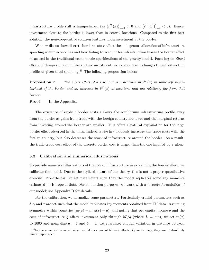
We now discuss how discrete border costs τ affect the endogenous allocation of infrastructure

spending within economies and how failing to account for infrastructure biases the border effect

measured in the traditional econometric specifications of the gravity model. Focusing on direct

effects of changes in τ on infrastructure investment, we explore how τ changes the infrastructure

profile at given total spending.29 The following proposition holds:

Proposition 7 The direct effect of a rise in τ is a decrease in iH (x) in some left neigh-

borhood of the border and an increase in iH (x) at locations that are relatively far from that

border.

Proof In the Appendix.

The existence of explicit border costs τ skews the equilibrium infrastructure profile away

from the border as gains from trade with the foreign country are lower and the marginal returns

from investing around the border are smaller. This offers a natural explanation for the large

border effect observed in the data. Indeed, a rise in τ not only increases the trade costs with the

foreign country, but also decreases the stock of infrastructure around the border. As a result,

the trade trade cost effect of the discrete border cost is larger than the one implied by τ alone.

5.3 Calibration and numerical illustrations

To provide numerical illustrations of the role of infrastructure in explaining the border effect, we

calibrate the model. Due to the stylized nature of our theory, this is not a proper quantitative

exercise. Nonetheless, we set parameters such that the model replicates some key moments

estimated on European data. For simulation purposes, we work with a discrete formulation of

our model; see Appendix B for details.

For the calibration, we normalize some parameters. Particularly crucial parameters such as

δ, γ and τ are set such that the model replicates key moments obtained from EU data. Assuming

symmetry within countries (m(x) = m, q(x) = q), and noting that per capita income b and the

cost of infrastructure q affect investment only through bL/q (where L = ms), we set m(x)

to 1000 and normalize q = 1 and b = 1. To guarantee enough variation in distance between

29In the numerical exercise below, we take account of indirect effects. Quantitatively, they are of absolutelyminor importance.

23

Table 2: Calibration strategy

(a) Normalizations

Parameter Value Explanation

m(x) 1000 arbitrary choices 500 arbitrary choiceb 1 symmetryq(x) 1 symmetryα 0.5 arbitrary choice

(b) Parameters calibrated to match EU data

Parameter Value Moment

γ 0.86 Distance elasticity of transport costs in French data(Combes and Lafourcade, 2005): 0.9

δ 1.65 Distance elasticity µ1 estimated in EU trade data: -1.1τ 1.32 Border effect µ2 estimated in EU trade data: -0.8σ 2.70 Set to satisfy (10) given calibrated values of γ, δ, τ

locations generated by the model, we set s at 500. We set the share of income spent on the

agricultural product, α, to 0.5.30

We set parameters δ, γ, τ such that the model replicates key empirical moments. To this

end, we apply a gravity equation of the type

lnXij = µ1 lnDij + µ2Bij + exi + imj + εij , (19)

to data generated by our model and to actual data. Xij represents trade volumes from location

i to j, Dij denotes the distance between the locations, Bij is a border dummy that is equal to

one if i and j belong to different countries, exi and imj are exporter and importer fixed effects,

and εij is the error term. We use European trade data to estimate the empirical counterpart of

(19); see Section 6. This yields estimates µ1 = −1.1 and µ2 = −0.8. We parameterize the model

such that the trade data generated from it produces exactly the same values for µ1 and µ2 as

those obtained from real data. The parameter γ is chosen such that the generated elasticity

of internal transportation costs with respect to distance matches the value of 0.9 estimated in

French data.31 We use parameter restriction (10) to set the elasticity of substitution σ at the

maximum admissible level.

Table 2 summarizes the calibration strategy and outcomes. The border friction implies an

ad valorem tax equivalent of 32%, which is a reasonable magnitude compared with estimates

30In Table 4 we report robustness checks pertaining to these choices.31We do not match spending on infrastructure investment t, because due to the one-period nature of our model

i(x) measures capital stocks while the empirical value of t discussed in Section 2 refers to the flow of (gross)investment.

24

presented in Anderson and van Wincoop (2004). The interregional elasticity of substitution is

1/δ = 0.61, implying a fairly strong degree of complementarity of investments between different

locations. The parameter governing the curvature of the transportation cost – distance relation-

ship is γ = 0.86. Finally, the maximum value of σ that satisfies the parameter restriction (10)

is 2.7.32 We use this parameterization as our benchmark configuration.

We are now ready to run numerical exercises. We start with the counterfactual situation

where τ is equal to unity. Figure 3 compares optimal schedules for infrastructure investment and

aggregate price levels, denoting the outcome under autarky by ia(x), the world-planner solution

by iw(x), and non-cooperative Nash outcome by (iH(x), iF (x)). In line with our analytical

results, the world-planner schedule has a unique maximum at the location of the border, while

the non-cooperative schedule has a double-hump shape with underinvestment around the border

(compared to the world-planner outcome). This shape generates a border effect even without

having any discrete border costs.

Figure 3: Infrastructure investment and price levels across space in the absence of explicit(discrete) border frictions (i.e., τ = 1)

(a) Investment (b) Price levels

Notes. ia(x), iw(x), and iH(x) refer to the autarky, central-planer, and non-cooperative optimal infrastructureinvestment distributions. Similarly for price levels. See Table 2 for the parameterization and Table 3 for numericalresults.

Panel b in Figure 3 depicts the distribution of the price index across locations in the autarky,

world-planner, and Nash outcomes. In our framework, the price index at location x depends

32This is a low value compared to findings in the literature; see Costinot and Rodriguez-Clare (2014) for asurvey. As equation (10) is only a sufficient condition, we can set σ at higher levels, but may end up violating the(unknown) necessary condition for the existence of an interior solution. We work with σ = 3.4 in the robustnesschecks below.

25

on the ‘remoteness’ of the location (which determines the level of ‘global’ trade) and the level

of infrastructure in the neighborhood (which determines the level of ‘local’ trade). Thus, in

the world-planner outcome the price index is the lowest at the border, since the border is the

least remote location in the world economy and the infrastructure investment is the highest

there. In contrast, in the Nash equilibrium the price index has the lowest value at some internal

location, rather than at the border (meaning that the local effect is stronger than the global

one). This is caused by the skewness of the infrastructure profile towards internal locations in

the Nash outcome. If we decrease the geographical size of countries s (making ‘local’ trade less

important), the lowest value of the price index will be closer to the border.

Given our parameterization, Table 3 shows that underinvestment in border regions is quan-

titatively quite substantial, while global underinvestment is not. Compared to the first-best

situation (row (2)), the non-cooperative outcome (row (3)) displays an investment gap of 49%

at the border (compare 88.5 to 172.9). Overall spending on infrastructure investment (measured

by the equilibrium tax rate), falls only 7% short of the first-best. Compared to autarky, invest-

ment is about 5% higher in the first-best situation but about 2% lower in the Nash equilibrium.

Real net per capita income at location x being given by W (x)= (1 − t)b/P (x), we use average

real per capita income, E[W ], as a measure of welfare (in Table 3 we normalize autarky welfare

to unity). The gains from trade are about 7.1% when the infrastructure investment schedule

is first-best and about 5.6% when it is Nash; the cost of non-cooperation therefore amounts to

about 1.4% of autarky welfare, or, equivalently to 20% of the gains from trade achievable when

investment is first-best.33 Interestingly, inequality (as measured by the variance of the log of

real net income multiplied by 100) is almost identical in autarky and in the first-best situation,

but is substantially lower in Nash, where the income differential between the border region and

the periphery is much smaller

In Figure 4 we set τ = 1.32. The world planner spends 4.5% more on infrastructure than

country-level governments would, while the shortfall of investment at the border is around 46%.

The welfare loss (the difference between the average real per capita income in the first-best

and non-cooperative outcome) constitute around 0.8%. This suggests that lower border frictions

increase the welfare loss from infrastructure misallocation (when τ = 1, the loss is around 1.3%).

The fall in the real income at the border is more substantial (around 8.7%), suggesting that the

33If we fix overall spending to the first-best level, but allow independent governments to decide about the spatialdistribution of this spending, the welfare losses become minor. This outcome is robust across different param-eterization, suggesting that welfare losses arising in case of the Nash equilibrium are mainly due to insufficientfinance (a lower tax rate), rather than the distribution of infrastructure itself. The border investment is higherwhen overall spending is forced to be at the first-best level, but it still falls short from the optimum substantially.

26

Table 3: Autarky versus first-best and Nash outcomes under trade

(1) (2) (3) (4) (5)border inv. max. inv. tax rate real income inequalityi (500) arg max i (x) t E [W ] V [lnW ] ,%

Autarky: τ =∞(1) ta, ia (x) 0.0 250 13.4% 1.0000 1,69

No discrete border frictions: τ = 1 (counterfactual)(2) tw, iw (x) 172.9 500 14.1% 1.0707 1.67(3) tH , iH (x) 88.5 296 13.1% 1.0563 1.20

Discrete border frictions: τ = 1.32 (data)(4) tw, iw (x) 117.6 322 13.8% 1.0419 1.24(5) tH , iH (x) 63.6 276 13.2% 1.0335 1.14

Notes: The parameterization is as in Figure 3. Two symmetric countries, S = [0, 1000].

Autarky welfare is normalized to unity.

welfare loss from underinvestment in infrastructure can be larger, if a country has more than one

border. The border cost decreases average real per capita income by around 2%. The presence

of the border cost τ also changes the distribution of the price index (see panel b of Figure 4).

If there is a border friction, the prices of the foreign varieties rise compared to the prices of the

local varieties and, infrastructure investment moves away from the border. As a result, the price

index achieves its minimum in more remote (from the border) locations. In the extreme case

with prohibitive border costs, we have the autarky case where the price index has a U -shape

with the minimum at the central location.

To assess the role of infrastructure in explaining the border effect, we perform the following

experiment. We set the infrastructure investment i(x) at all locations to its average value under

the benchmark parameterization i (which is 131.8). In this case, the distribution of infrastructure

is flat and does not affect the size of the border effect. All other parameters and variables remain

fixed. Then, we simulate trade volumes within and between countries and estimate the border

effect generated by the model. We find that the estimate of µ2 drops from 0.80 to 0.65. This

means that the variation in infrastructure investments explains around 19% of the border effect.

The rest is explained by the border friction τ and the correlation between the border dummy

and distance generated by the model.34 In other words, the border effect identified in a gravity

model that ignores variation in transport infrastructure over space is biased upward by 19%.

The discrete border friction τ = 1.32 explains about 59% of the border effect, and 22% is due

34That correlation amounts to 71%. It arises from the fact, that pairs of locations characterized by shortdistances tend to be within-country and, thus, have a border dummy of zero while the opposite is true for longdistances.

27

Figure 4: How higher discrete border costs change the distribution of infrastructure investmentand price levels across space

(a) Investment (b) Price levels

Notes. iH(x) and iF (x) refer to the non-cooperative (Nash) infrastructure investment distributions, and iH′(x)and iF ′(x) show the same loci with a higher border cost. See Table 2 for the parameterization and Table 3 fornumerical results.

to the correlation between the border dummy and distance.35

We also perform robustness checks regarding the chosen values of m(x), s, n, and σ. In

particular, we change the value of one of these parameters, re-calibrate the model, and assess

the role of infrastructure in explaining the border effect as well as the size of welfare losses.

Table 4 summarizes the results. As can be seen, a rise in the population density (see row (1) in

the table) barely changes the calibrated values of γ and τ and the welfare losses. The value of δ

decreases from 1.65 to 1.50. Since the value of δ falls, the variation in infrastructure investments

becomes less important and, consequently, the role of infrastructure in explaining the border

effect becomes less pronounced. In contrast, an increase in the geographical size of countries

s (row (2)) raises the value of δ and, thereby, increases the role of infrastructure. The values

of γ and τ and the welfare losses do not substantially change. A decrease in the number of

internal regions n from 100 to 70 (row (3)) has a minor impact on the values of the calibrated

parameters, welfare losses, and the role of infrastructure. Finally, a rise in σ (row (4)) has a

substantial impact on the calibrated values of the parameters (especially, on τ), while the impact

on the role of infrastructure and welfare losses is small. The role of infrastructure increases from

19% to 22% and the welfare losses increase from 0.8% to 1%.

35This as a statistical artefact that arises from the high correlation between distances and the border dummy.It implies that if i(x) = i and τ = 1, the model still generates a statistical border effect.

28

Table 4: Robustness checks

(1) (2) (3) (4) (5)γ δ τ 4W Infra

Benchmark:m(x) = 1000, s = 500,n = 100, σ = 2.7

0.86 1.65 1.32 0.8% 19%

(1) m(x) = 10000 0.85 1.50 1.35 0.7% 13%(2) s = 700 0.86 1.69 1.31 0.9% 21%(3) n = 70 0.86 1.66 1.32 0.9% 20%(4) σ = 3.4 0.80 1.83 1.12 1% 22%

Notes: We fix the moments measured in European and French data, modify our choice

of free parameters, and obtain new calibrated values for γ, δ, τ , (columns (1), (2), (3)).

Columns (4) and (5) show the welfare costs resulting from an inefficient infrastructure

investment, and the relative importance of infrastructure in explaining the border effect,

respectively.

5.4 The role of country asymmetries

We study asymmetries with respect to countries’ populations (given area), or with respect to

areas (holding population constant). Figure 5 illustrates these cases, where Home is always

assumed the ‘bigger’ country, and we distinguish between cases with and without an explicit

discrete border friction τ . In panels a and c, both countries have the same geographical extension,

but Home has a higher population (and, hence, a higher density). Specifically, we set mH(x) =

1100 and mF (x) = 900.36 In panels b and d, Home has a larger geographical extension, but

the same density m(x) as Foreign. The figures show that, regardless of whether or not there

is a discrete border cost and regardless of the nature of the asymmetry, the larger country

wishes to invest more (in the sense that the mode of the distribution is higher). However, in

contrast to the symmetric case, the planner solution involves a concentration of investment in

the ‘bigger’ economy; with an explicit border friction, the planner solution can even be bimodal

(panel d). In all cases, the Nash equilibrium yields global underinvestment, including at the

border. However, the spatial structure differs across scenarios.37 The ‘bigger’ country severely

underinvests, but the ‘smaller’ one may overinvest relative to the planner solution. This is

particularly pronounced when the source of asymmetry is density; in this case, the location with

the strongest underinvestment typically is an interior location in Home. When asymmetry is

caused by geographical size, the extent of underinvestment is strongest in the border region.

Interestingly, overinvestment in Foreign under Nash implies that the smaller country may

36Compared to the benchmark configuration with mH(x) = mF (x) = 1000, world income expressed in thenumeraire is the same.

37In the Nash equilibrium, the infrastructure investment profile has a discontinuity at the border (caused bythe asymmetry between the countries).

29

Figure 5: The distribution of infrastructure investment when Home is ‘bigger’ than Foreign

(a) Population size (τ = 1) (b) Geographical size (τ = 1)

(c) Population size (τ = 1.32) (d) Geographical size (τ = 1.32)

Notes. iH(x) and iF (x) refer to the non-cooperative and iw(x) to the central-planer and optimal infrastructureinvestment distributions. The default parameterization follows Table 2. Panels (a) and (c): m(x) is 1100 and 900for domestic and foreign locations, respectively. In the non-cooperative outcome with τ = 1.32, the tax rate is13.2% in Home and 13.3% in Foreign. Average real per capita income is 8.87 and 8.37, respectively. The levelof inequality is 1.15 and 1.13. Panels (b) and (d): The geographical size of Home and Foreign is 750 and 250,respectively. In the non-cooperative outcome with τ = 1.32, the tax rate at Home and Foreign is 13.8% and12.0%, respectively. Average real per capita income is 8.87 and 8.08, respectively. The level of inequality is 1.16and 1.01.

gain from non-cooperation (assuming away any transfers between countries in the first-best

outcome). In panel c, in the first-best outcome, average real per capita income at Foreign is

7.04, while in the Nash outcome it is 8.37, i.e., non-cooperation outperforms cooperation by

around 19%. In contrast, Home’s average income is 9.74 the first-best outcome, while it 9%

lower under Nash (8.87). Hence, asymmetry in population density across countries may increase

the welfare losses (caused by the misallocation of infrastructure in the Nash equilibrium) of the

30

larger country and decrease those of the smaller country (that may even gain). Thus, under

asymmetry, welfare effects of non-cooperation are substantially more substantial than in the

symmetric case (where the average welfare loss was just about 0.8%). A similar observation

emerges in panel d, where Home’s welfare loss under Nash relative to the first-best is around

2.7%, while Foreign gains around 6% from non-cooperation.38

5.5 Intercontinental trade

So far, we have studied a world of two countries which are connected by land-borne trade. Now

we study how the emergence of intercontinental trade affects the intracontinental distribution

of infrastructure investment, trade, welfare, and the size of the border effect. We do this by

assuming that there is a third country, call it China, which supplies and demands goods to and

from Home and Foreign via a harbor that is located at address 0 in Home. We also assume

that China’s supply and demand capacity is exogenous to the outcomes in Home and Foreign.

In particular, we do not model the spatial extension of China, and treat it as a mass point at

location 0.

By construction, this constellation creates a costal country (Home) and a hinterland (For-

eign). It also breaks symmetry between Home and Foreign, as any location in Home now is

more central than any region in Foreign, even with a uniform distribution of infrastructure in-

vestment: on average, consumer prices will be lower in Home than in Foreign. However, with

endogenous infrastructure investment, there will be additional effects that tend to exacerbate

inequality both between Home and Foreign as well as within them.39

Panels (a) and (b) in Figure 6 show how the intracontinental infrastructure investment

distribution changes due to the emergence of intercontinental trade with China. In panel (a)

China is considered to produce the same number of varieties as Home and Foreign together (that

is, it has the mass of 1000). In this case, the share of trade volumes from China to Home and

Foreign in the total income of those countries constitutes around 10%,40 reflecting the share of

imports (in total income) of EU from the rest of the world in 2010. In Home, there will be a

massive reallocation of spending towards the coastal locations where the Chinese imports crowd

38We also consider the case when both countries have the same total income with Home being larger in ageographical size, but less densely populated (the world total income remains fixed). In this case, we findthat Foreign loses from non-cooperation, while Home gains. This suggests that the effect of population densityon welfare losses is stronger than that of the geographical area. A number of robustness checks confirm thisconclusion.

39Another application of this model variant may be to poor coastal countries in Africa, which trade mostlyintercontinentally, and where intracontinental infrastructure and trade are underdeveloped.

40Such a low share (taking into account the size of China) is explained by the remoteness of China and the factthat only (1− α) share of total income is spent on industrial goods.

31

out varieties from locations within Home and Foreign. Investment falls rapidly with increasing

distance from the harbor and is lower than in the benchmark case (intracontinental trade only)

in about 80% of all locations in Home. In particular, Home will invest substantially less at the

border with Foreign. With the infrastructure schedule dramatically more skewed in Home, the

distribution of real wages will also become more uneven, so that trade with China makes Home

a more unequal economy.

Figure 6: Overseas trade and the distribution of intracontinental transport infrastructureinvestment

(a) “Large China” (b) “Small China”

Notes. iH(x) and iF (x) refer to the Nash infrastructure investment distributions without a third country, whileiH′(x) and iF ′(x) refer to those when there is trade with a third country (China). The parameterization is asfollows: σ = 2.7, δ = 1.65, γ = 0.86, α = 0.5, q(x) = q = 1, b = 1, τ = 1.32, m(x) = 1000 for all locations atHome and Foreign, and s = 500. In Panel (a) China has the mass of 1000, in (b) it has the mass of 40.

Simulations show that in Foreign, now a hinterland, incentives for investment barely change,

because there are two competing factors: On the one hand, all else equal, the presence of

China should result in more investment. On the other hand, this effect is mitigated by the

remoteness of China and the reallocation of infrastructure investment in Home away from the

border with Foreign. However, the emergence of China increases the intracontinental border

effect, because it diverts investment away from the border zone. This means that, in a standard

gravity equation, the estimated border dummy should grow larger with the increasing importance

of intercontinental trade despite the fact that border related trade costs have not changed.

Specifically, under the benchmark parameterization the presence of China increases the size of

the border effect by around 24% (from −0.8 to −0.99).

In panel (b) of Figure 6, we consider the case when China is much smaller than Home and

32

Table 5: The Presence of China: Inequality and Welfare

Home Foreign

Welfare Inequality Tax rate Welfare Inequality Tax rate

The size of China is 0: 1.0000 1.14 13.2% 1.0000 1.14 13.2%

The size of China is 40: 1.0243 0.26 13.2% 1.0000 1.14 13.2%

The size of China is 1000: 1.4658 33.62 11.2% 0.9949 1.25 13.1%

Notes: Calibration as in Table 2; ‘China’ is modeled as a mass point at location 0.

Welfare when the size of China is zero is normalized to unity.

Foreign (with a mass of 40). In this case, the infrastructure profile at Home still has a hump

shape. However, there is more investment in coastal areas and less in the hinterland compared

to the benchmark case (of intracontinental trade only).

A rise in trade with China increases welfare in the coastal country but has minor effects

in the hinterland (Foreign), where inequality also remains essentially unchanged. In contrast,

trade with China has a substantial non-monotonic effect on inequality in Home. When the size of

China is small, inequality in Home decreases (since the distribution of the infrastructure becomes

flatter (see panel b in Figure 6)). When China is big, inequality rises, as the infrastructure profile

is highly skewed towards the border with China (see panel a in Figure 6). Table 5 summarizes

the effects of trade with China on Home and Foreign under the benchmark parameterization.

6 Supporting evidence

Two important prediction of our theoretical model are: (i) locations within jurisdictions are

better connected by transport infrastructure than locations lying in two different jurisdictions,

and (ii) inefficiently low infrastructure investment in border regions explains part of the so called

border effect. In this section we use data from the European Union to provide some supporting

evidence for these hypotheses.

Data. We use data provided by Pisu and Braconnier (2013) on bilateral minimum road dis-

tances and minimum travel times between 220 cities in 22 countries in continental Europe.41

The data come from Bing Maps Route Service and relate to the year 2012. The authors provide

41The countries are: Austria, Belgium, Bulgaria, Czech Republic, Denmark, Estonia, France, Germany, Greece,Italy, Hungary, Latvia, Lithuania, Luxembourg, Netherlands, Poland, Portugal, Romania, Slovenia, Slovak Re-public, Spain, Switzerland.

33

population weighted proxies at the country-pair level which we use in our analysis. We merge

this information with bilateral trade data for the year of 2010 provided in the World Input

Output Database (WIOD) project (Timmer et al., 2015). Crucially, that data base provides

accurate measures for domestic trade within countries. Unfortunately, there is no information

on Switzerland, so that our analysis rests on 212 = 441 country pairs. We focus on the 16

non-service sectors contained in WIOD. Finally, we obtain CES weighted geographical distance

measures (based on great-circle distances), common language and contiguity measures from

Mayer and Zignago (2011).42

Straight-line distance, road distance, and travel time. We start by showing direct evi-

dence on relative underinvestment in European border regions. The left-hand diagram in Figure

7 shows that the ratio of road distance to the straight-line distance (the so called divergence)

is on average higher between cities in different countries than between cities within the same

country. Intranational road trips are 9% longer than what the great-circle (bird-flight) distance

would indicate; international road trips are 30% longer. The difference is statistically significant

at the 1% level. As the mid panel in Figure 7 shows, the average travel speed on domestic roads

is 88 km/h while it is 100 km/h on international road trips; the difference again being significant

at the 1% level. However, this disadvantage for domestic trips does not outweigh the advantage

of shorter connections. The hypothetical speed of traffic for overcoming the bird-flight distance

is 83 km/h in domestic links versus 77 km/h in international links. This difference is statistically

significant at the 5% level.43

Table 6 conditions the difference between domestic and international trips on distance and

also controls for destination and origin fixed effects. Column (1) reports a simple linear regression

that correlates the log of travel time (in minutes) and the log of geographical (great-circle)

distance. The obtained elasticity is 0.96. Moreover, column (2) shows that travel time is

significantly larger between different countries than within countries, the difference being equal

to about 28%. Including the dummy variable for domestic connections brings down the elasticity

of travel time with respect to distance to 0.89, again hinting at some concavity in the relationship

between distance and trade costs.44 Columns (3) and (4) repeat this exercise, but use the log of

road distance (in km/h) as the dependent variable. It turns out that road distances that cross

42Head and Mayer (2002) show that measuring distance between countries by a geometric (CES) average ofdistances between major cities dramatically reduces the border effects in European data. These authors, however,do not account for real transportation costs.

43Note that the hypothetical travel speed on the bird-flight distance is given by the ratio between the travelspeed on the road and the excess length of the road trip over the bird-flight distance.

44The hypothesis of a unitary elasticity is rejected at the 1% level.

34

Figure 7: Distance versus travel time in intra- and international bilateral links

050

100

150

International Intranational

Avg. excess distance (%)

050

100

150

International Intranational

Avg. road speed (km/h)

050

100

150

International Intranational

Avg. direct speed (km/h)

Notes. Average excess distance is the %-ratio between road distance and bird-flight distance, both in km. Avg.road speed denotes the average travel speed on the fastest road connection, in km/h, while avg. direct speedrefers to the average theoretical speed on the most direct (= bird-flight distance), in km/h.

a political border are longer by some 22%, controlling for bird-flight distance. Finally, columns

(5) and (6) show that domestic travel time is longer by 8% given road distances.

The border effect. Finally, we turn to an investigation of the border effect. To this end, we

use a generalization of equation (19)

Xijs = exp [µ1 lnTij + µ2Bij + exis + imjs + εijs] ,

where s indicates the sector. Bilateral trade costs are Tij and Bij , where the latter is a dummy

that takes value one if for an international and value zero for an intranational transaction. Tij =

(1 +Dij)δ0 eδ1CLij+δ2CONTij models trade costs as a function of distance-related transportation

costs Dij , common language CLij and contiguity CONTij . Dij can either be the weighted

great-circle distance between i and j, or the shortest (similarly weighted) road distance, or

the minimum (similarly weighted) travel time. Following current practice, we estimate Poisson

models, as this setup is best suited do deal with zero trade flows and heteroskedasticity arising

from additive error terms.45

45See Head and Mayer (2014). As a default, we use a Poisson pseudo maximum likelihood estimator (PPML),but for the instrumental variable estimation we estimate the Poisson model using a a generalized methods ofmoments (PGMM) approach. Note that results do not qualitatively depend on using the Poisson approach.Log-linear OLS models yield qualitatively similar results; see Table 9 in the Appendix.

35

Table 6: Bird-flight distance, road distance, and travel time across EU countries

(1) (2) (3) (4) (5) (6)Dep.var.: log travel time log road distance log travel time

Border (0,1) 0.282*** 0.217*** 0.0799***(0.0418) (0.0325) (0.0232)

ln bird-flight distance 0.959*** 0.893*** 1.041*** 0.990***(0.0137) (0.0128) (0.0113) (0.00945)

ln road distance 0.924*** 0.905***(0.0104) (0.00987)

Constant -0.0795 0.344*** -0.0253 0.300*** -0.0721 0.0526(0.0890) (0.0837) (0.0727) (0.0613) (0.0682) (0.0657)

R-squared 0.983 0.986 0.992 0.994 0.994 0.994

Notes: OLS regressions. All regressions contain complete sets of separate exporter and importer fixedeffects. Robust standard errors (clustered at the pair-level) in parentheses, *** p < 0.01, ** p < 0.05, *p < 0.1. N = 441.

Table 7: The border effect and the role of infrastructure: Poisson models

(1) (2) (3) (4) (5) (6) (7) (8) (9)Dep.var.: aggregate trade sectoral tradeSample full non-contingent pairs full

PPML PPML PPML PGMM PGMM PGMM-IV PPML PPML PPML

Border (0,1) -0.804*** -0.547*** -0.422** -2.063*** -1.546*** -1.411*** -0.775*** -0.503*** -0.391***(0.170) (0.180) (0.176) (0.458) (0.428) (0.462) (0.0915) (0.101) (0.101)

ln great-circle distance -1.112*** -1.204*** -1.142***(0.128) (0.135) (0.0674)

ln road distance -1.171*** -1.211***(0.123) (0.0693)

ln travel time -1.361*** -1.365*** -1.443*** -1.391***(0.124) (0.139) (0.163) (0.0713)

Common language (0,1) 0.761*** 0.840*** 0.841*** -0.295 -0.145 -0.134 0.763*** 0.843** 0.841***(0.132) (0.134) (0.125) (0.414) (0.355) (0.367) (0.0803) (0.0793) (0.0792)

Contiguity (0,1) 0.326** 0.215 0.134 0.320*** 0.200** 0.131(0.157) (0.154) (0.141) (0.0845) (0.0843) (0.0816)

Constant 14.92*** 15.58*** 16.07*** 17.66*** 17.66*** 18.03*** 12.49*** 13.24*** 13.63***(0.881) (0.872) (0.802) (0.835) (0.835) (0.834) (0.780) (0.788) (0.758)

Observations 441 441 441 377 377 377 7,004 7,004 7,004R-squared 0.989 0.990 0.991 0.977 0.977 0.959 0.961 0.961

Notes: Pseudo Maximum Likelihood (PPML) or Generalized Methods of Moments (PGMMs) estimations of Poisson moels. All models contain complete

sets of separate exporter and importer fixed effects (exporter × sector, importer × sector effects in case of sectoral trade data). Robust standard errors in

parentheses, *** p < 0.01, ** p < 0.05, * p < 0.1.

36

Column (1) of Table 7 reports a frequently observed pattern in gravity models: the trade

elasticity of bird-flight distance is close to −1, and a common language or a adjacency (contigui-

ty) have strongly positive effects on trade flows. The estimated border effect is −0.804, signalling

that international trade flows are by about 55% (1− exp(−0.804) = 0.55) smaller than intrana-

tional ones, holding other trade determinants (such as market sizes, multilateral distances – all

captured by fixed effects – geographical distance, contiguity, and common language) constant.46

Using the log of road distance or travel time instead of great-circle distance as a proxy of

transportation costs (columns (2) and (3)), the estimated border effect increases from −0.804 to

−0.547 and to −0.422, respectively. Hence, international trade is only by 42% and 34% smaller,

respectively, than intranational trade, holding other determinants of trade constant.47 Hence,

it appears that, in Europe, using proxies of transportation costs that account for the quality of

infrastructure brings down the estimated border effect by between 24% and 38%.

Sensitivity Analysis. Treating borders as exogenous to sectoral trade shocks εijs, the iden-

tification assumption underlying our analysis can be stated as cov (εijs, Tij |Bij , exis, imis) = 0.

A high realization of εijs could incite countries i and j to invest into reducing Tij , which could

bias the distance effect µ1 away from zero. How this affects our coefficient of interest, µ2, is

not obvious, though. Tij depends on investment Ii and Ij , but also on investment by countries

k 6= i, j located on the shortest travel route between i and j. So, if i and j boost investment due

to a positive shock in εijs, they also lower Tii and Tjj , which increases Xii and Xjj , and this

contributes to moving µ2 upwards at given Ik.

To contain the danger of biased results, we restrict the sample to non-contingent countries,

the transport links between which are importantly shaped by countries other than the trade

partners themselves. We also instrument trade costs Tij by the weighted sum of Tkk, where

k belongs to the set K of countries through which any transport from i to j has to transit.

More precisely, we focus on travel time and apply the average travel speeds measured in within-

country k ∈ K links to the great-circle distance from i to j. The partial correlation between this

instrument and actual travel time Tij is 0.46. Columns (4) to (5) of Table 7 show the results.

First, note that excluding the 61 contingent pairs strongly increases the absolute value of the

46The measured border effect seems small compared to earlier findings in the literature, e.g., by Nitsch (2000).This has several reasons: First, we use the more consistent distance measure proposed by Head and Mayer(2002), which has been shown to shrink the border effect in a sample of European data from the early 1990s (seefootnote 42). Second, the use of PPML yields a substantially smaller border effect than OLS, which dominatedthe earlier literature; compare Table 9 in the Appendix. Third, thanks to the WIOD project, we have moreaccurate information on within-country trade. And fourth, our data refers to a very recent period (2010) andlower border effects probably simply show the effects of ongoing economic integration in the EU.

471− exp (−0.547) = 0.42, and 1− exp(−0.422) = 0.34, respectively.

37

border effect (column (4)).48 Second, replacing great-circle distance by travel time lowers the

absolute value of the border effect quite significantly (column (5)).49 Third, instrumenting travel

time further slightly reduces the absolute value of the border effect but increases that of travel

time (column (6)).

Next, we turn from aggregate to sectoral data. Columns (7) to (9) show that our argument

remains robust. Estimated coefficients change only minimally. If we drop all trade relationships

of any country that account for more than 5% of total sector-level trade and which are, thus

presumably important enough to affect investment decisions, we find a substantially higher

border effect, but replacing great-circle distance by road distance or travel time shrinks the

effect; see Table 10 in the Appendix.50

Finally, we also check whether our results are driven by the recent eastward enlargement

of the EU. Excluding the 10 new eastern European EU member countries present in our data,

we find an algebraically smaller border effect. Still, the measured border effect changes upon

replacing great-circle distance by road distance or travel time in the way suggested by our model.

7 Extensions and robustness analysis

In this section, we discuss some potential extensions of the framework.

7.1 Toll roads

Today, many countries operate public toll tax systems for freight traffic. The share of interre-

gional highways subject to decentrally administered toll systems ranges from 6 percent in the

U.S. to 52 percent in France. Countries such as Germany and Austria have centrally adminis-

tered distance dependent road pricing for lorries. User fees may be contingent on a wide array

of factors such as the situation of the environment (e.g., smog), the degree of congestion, the

time at which a road is traveled, and so on.

How a toll system affects the main argument in this paper depends very much on its specific

design. Here we study a particularly interesting and relevant configuration. Suppose govern-

ments decide on the infrastructure allocation across space, but rather than taxing consumers

48The common language dummy turns insignificant as we have only very few non-contingent countries withcommon language in the sample.

49A similar result obtains when using road distance; see Table 10 in the Appendix. Interestingly, the elasticityof trade with respect to travel time is almost unchanged by restricting the sample to non-contingent pairs.

50Table 11 in the Appendix runs sector-level regressions and finds statistically significant border effects in 12out of 16 sectors. In all of these sectors, the border effect is (algebraically) smaller when road distance or traveltime is used instead of great-circle distance.

38

through lump-sum taxes, they tax road users per unit of distance. Further assume that the tax

varies continuously on the space of addresses and that it works just as our iceberg transportation

costs, albeit with the shaved transported good not lost but transferred into the governments

coffers and redistributed to households. In that case, the government has two margins of action:

it sets a distribution of fees, f (s), where s ∈ [0, s], and decides on the infrastructure allocation,

i (s) . Total income from fees will be B =∫ s

0 f (s) R (s) ds, where R (s) measures total traffic

through location s. Note that R (s) depends on the domestic and on the foreign distribution of

infrastructure. If the government is free to spend B on whatever infrastructure distribution it

prefers, and does not impose any additional tax, it will find it optimal to make fees dependent

on the distance to the border, with higher fees the closer the border. Moreover, it will concen-

trate its spending as before in the central regions of the jurisdiction. The reason for this result

is identical to the one discussed above: The government cares only about home welfare, thus

taxing foreigners and transferring the receipts to home citizens is a welcome option.

If governments are not allowed to spend toll income on places other than those where the

income has been generated, there will be a direct link between infrastructure investment and

transit volume, f (s) R (s) /q (s) = i (s) . Governments will then set f (s) such that native welfare

is maximized. By imposing high fees in border regions, governments tax foreign consumers more

strongly than domestic ones; however, the implied high investment volumes are of little value

for domestic consumers. By imposing high fees in the center, governments affect domestic

consumers, but also achieve high utility for them. The implied distribution of infrastructure

need not exhibit excessive spatial variation, but it still can; the exact outcome depending on

underlying model parameters.

7.2 Private-public partnerships (PPP)

Since ancient times, governments have asked private agents to construct and operate roads or

railways and allowed them to take fees for road usage. In England, from the 17th century

on, Parliament entrusted private companies with concessions to run certain road connections;

around 1830 there were about 48,000 km of so called turnpike roads; see Lay (1992). The system

was also used in the US. Currently, cash-strapped governments around the world use various

types of PPP to finance the construction of transport links.

We provide a simple model of such a situation. Each government in the two countries auctions

the exclusive right to run a road segment which coincides with the space of the government’s

jurisdiction. The firm with the highest bid gets the license. In a competitive auction, the

39

equilibrium bid amounts to exactly the profits that the would-be monopolist can achieve. In

principle, the government can let the monopolist choose the preferred investment schedule i (s)

and a fee structure f (s) . Or it can regulate either i (s) or f (s) . Here, we consider an example

where two contiguous countries each entrust a private monopolist to choose an optimal iM (s),

given a regulated user fee p per unit of traffic.

The monopolist in Home sets iM (s) to maximize profits

π(iM)

= p

∫ s

0R(x)dx−

∫ s

0q(x)iM (x)dx, (20)

where R(x) is the measure of the total traffic through location x, iM (x) is infrastructure invest-

ment at location x, and q(x) denotes the associated cost per unit of investment.51

Total traffic through location x is given by

R(x) =

∫ x

0

(∫ 2s

xR(y, z)dz

)dy +

∫ 2s

x

(∫ x

0R(y, z)dz

)dy,

where

R(y, z) = (1− α)(1− tM )Y (z)T (y, z)1−σ∫ s0 T (v, z)1−σ dv

.

Here, R(y, z) is interpreted as the traffic from y to z: a quantity measure of trade in products

produced at y and transported to z. It is determined by demand at location z and the trans-

portation costs from y to z. Note that in general R(y, z) is not equal to R(z, y). Finally, tM is

the income tax imposed by the government to finance the infrastructure investments and Y (z)

is the gross income at location z. We assume that the monopolist takes the income tax and

the location sizes as given. As in the benchmark case, the monopolists at Home and Foreign

choose the corresponding infrastructure investments non-cooperatively. In the symmetric Nash

equilibrium with no asymmetries in the cost of infrastructure and the location size, the domestic

infrastructure profile (in case of the interior solution) is given by

ıM (x)δ =pγ(1− α)(1− tM )(σ − 1)

q

(φL,M

(x) + φR,M

(x)),

where as before φL,M

(x) (φR,M

(x)) represents the aggregate marginal profits due to a rise in

traffic from the right (the left) to the left (the right) of location x.

51In the above specification, we assume that the government pays a fixed price p per unit of the traffic to themonopolist and finances this with a lump-sum tax. This assumption removes the distortive effects of p on theinfrastructure profile.

40

Similar to the social-planner scenario, the monopolist infrastructure profile has a hump shape

in autarky and is skewed towards the border with the foreign country in the open economy

case. It is also straightforward to show that the presence of costs associated with crossing the

border will redistribute the infrastructure away from the border, amplifying the border effect.

However, there is a conceptual difference between iH (s) and iM (s) . Under certain parameter

constellations, the monopolist finds it optimal to chose zero investment in peripheral locations.

This is because higher investment in s has two effects on total traffic. On the one hand, traffic

through s goes up, increasing total traffic. On the other hand, traffic through other regions goes

down because of the corresponding changes in the price indices (a substitution or trade diversion

effect). This tends to decrease total traffic. In some cases the negative effect prevails over the

positive one, so that iM (s) = 0. In contrast, the social planner sets i (s) > 0 for all s except

s = 0.

Figure 8 shows the optimal infrastructure distributions chosen by the monopolists under

autarky (panel a), and under international trade (panel b), and compares them with the Nash

social-planner or the first-best solutions. The parameterization is benchmark with τ = 1 and the

fee p is set such that the monopolist and social-planner scenarios yield the same overall invest-

ment. As can be seen, the monopolist chooses investment schedules that exhibit substantially

more spatial variation than the one picked by the social planner. Moreover, as discussed above,

there is zero investment at peripheral locations in both panels. In the case of international trade,

the monopolist invests much more around the border even compared to the first-best outcome.

This can generate a smaller or even no border effect, but comes at cost of zero investments in

many peripheral locations (that are in fact driven into autarky).

7.3 Internal labor mobility

In the model we assume away the effects of internal labor mobility on the infrastructure profile.

Here we offer some discussion. First, note that the underinvestment problem in border regions

relative to the first-best occurs regardless of the form of a (non-degenerate) distribution of

economic activity. This is because the share of non-internalized benefits of investment are

higher the closer one gets to the border, regardless of distributional details.

In contrast, how the endogenous adjustment of infrastructure investment shapes the distri-

bution of economic activity and the size of the border effect, is hard to determine analytically

as the social planner needs to internalize the effects of infrastructure on the endogenous popula-

tion density. Moreover, multiple equilibria are possible. At the same time, the intuition behind

41

Figure 8: Equilibrium investment loci: social planner vs. monopolist.

(a) Autarky (b) Trade

Notes. Solid black curves (iM (x) and iMH(x)) refer to investment profile resulting from non-cooperative mo-nopolists. Dashed red curves (ia(x) and iH(x)) refer to (non-cooperative Nash) solutions. The parameterizationis as follows: σ = 2.7, δ = 1.65, γ = 0.86, τ = 1, α = 0.5, q(x) = q = 1, b = 1, m(x) = 1000 for all locations, ands = 500. In Figure (a), p = 0.4. Spending on infrastructure (in terms of the tax rate) in this case is 13.4 percent.In Figure (b), p = 0.275. Spending on infrastructure in each country in the Nash equilibrium is 13.1 percent.

the impact of labor mobility on the equilibrium infrastructure profile seems to be relatively

straightforward.

With internal labor mobility (associated with some adjustment costs to avoid extreme solu-

tions), the equilibrium can be considered as the outcome of the following multi-stage variation of

the model. The economy starts with some distribution of population, which results in a certain

distribution of infrastructure investment chosen by the social planner. Then, given this infras-

tructure profile, agents decide about their location and, as a result, the population distribution

changes. Given the new distribution of population, the social planner adjusts the distribution

of infrastructure and continues doing so until convergence.

To understand the potential effects of labor mobility on the infrastructure profile in the above

variation of the model, we distinguish between high and low border frictions, and we assume a

uniform distribution of population as the initial one. With relatively high border costs, after the

first stage, the distribution of the price index will have a U -shaped form with the minimum at

some internal location that is relatively close to the central one (see panel b in Figure 4). In this

case, at the second stage the population will move away from the border to benefit from lower

aggregate prices at internal locations. This in turn will move the infrastructure distribution

even further from the border as well and so on. As a result, labor mobility will magnify the

concentration of infrastructure around internal locations and, therefore, increase the magnitude

42

of the border effect. The opposite happens when the border frictions are low. When the border

cost is low, after the first stage the price indexes will be the lowest relatively close to the border

(but not necessarily at the border as showed by the simulations), implying that the population

will move closer to the border. This will lead to more investment around the border and so on.

In this case, labor mobility will magnify the concentration of infrastructure around the border

and, thereby, decrease the magnitude of the border effect. However, underinvestment in Nash

relative to the first-best in border regions will remain, regardless of the distribution of economic

activity.

The reasoning above suggests that there can exist a certain threshold value of the border cost

τ such that if τ > τ , labor mobility increases the border effect, otherwise the opposite happens.

Further (perhaps, quantitative) analysis is needed to explore the actual effect of labor mobility on

infrastructure investments. Meanwhile, if the infrastructure investments were initiated/started

in the past when the border costs were quite high, then in the model with labor mobility one

might expect a higher border effect, rather than a lower one.

7.4 The political economy of infrastructure investment

An alternative way of modelling the endogenous infrastructure distribution is a majority rule

voting system. For any distribution of the transport infrastructure, each household derives a cer-

tain utility level which is represented by its indirect utility function. As a result, each household

has its own preferences over the continuum of infrastructure distributions that are determined

by the geographical location of this household: a household prefers more infrastructure invest-

ments around its location. For instance, for a household located at the periphery (x = 0),

the optimal infrastructure profile on [0, s] is a decreasing curve with maximum at x = 0. It is

possible to show that the household preferences defined above are single peaked. As a result,

the political equilibrium infrastructure profile is the profile chosen by the median voter, which

is the household located at x = s/2. So, in the absence of asymmetries across locations, the

median household will choose a hump shaped profile with maximum at s/2. In other words, the

median voter solution is qualitatively equivalent to the social planner solution. Thus, all the

qualitative results derived in the paper can be extended to the framework with a majority rule

voting system.

43

8 Conclusions

This paper develops a simple theoretical model where consumers demand goods from the entire

world, but the world is fragmented into jurisdictions which set infrastructure investment sched-

ules in a non-cooperative way. Governments care only for the welfare of their own constituency

and ignore the effects that their decisions have on foreign consumers; this basic externality leads

to global underinvestment. The lower the geographical distance of a location is to the political

border, the bigger is the externality since a larger share of the benefits caused by investment

accrues to foreign consumers. Hence, the externality has a spatial structure: infrastructure un-

derinvestment is stronger in poltically peripheral regions of jurisdictions rather than in central

ones.

The local lack of infrastructure investment makes imports from other countries more expen-

sive than imports from other regions from the same country, even if geographical distance or

incomes of trading partners are the same. Our infrastructure story may therefore contribute

towards unpacking trade costs and explaining the border effect first highlighted by McCallum

(1995) and since then discussed in a voluminous empirical literature.

We use intra- and international trade flows data from Europe to calibrate the model. We

find that about 20% of the empirically observable border effect is due to low infrastructure

investment around national borders. In our simulations, the border effect is magnified by the

emergence of intercontinental trade and appears larger, when countries are asymmetric with

respect to their sizes. We argue that privatization of construction and operation of roads may

not undo the border underinvestment problem; similarly, it also emerges under a majority voting

system.

Information from the Bing Maps Route Service allows us to show that international road

distances are about 22% longer than intranational ones and that travel is 28% longer, holding

bird-flight distance constant. The econometrically identified border effect falls from -0.80 in a

conventional setup to -0.55 when road distance is used rather than bird-flight distance. Hence,

using transportation cost proxies that account for infrastructure brings down the border effect,

as implied by our theoretical argument.

Future work should endogenize the distribution of economic activity by allowing intranational

migration of workers or/and firms. Moreover, to carry out a full-fledged quantitative analysis, it

would be needed to carry out the analysis on a plane rather than a line with realistic topology

as in Allen and Arkolakis (2014); this is a non-trivial generalization, since it requires not only

to characterize optimal investment schedules for given routes, but also to solve for the layout of

44

optimal transportation networks.

45

References

Allen, T. and C. Arkolakis (2014). Trade and the Topography of the Spatial Economy. Quarterly

Journal of Economics, 129(3): 1085-1140.

Anderson, J.E. and E. van Wincoop (2004). Trade costs. Journal of Economic Literature, 42:

691-751.

Anderson, J.E. and E. van Wincoop, E. (2003). Gravity with Gravitas: A Solution to the Border

Puzzle. American Economic Review 93(1): 170-92.

Behar, A. and A. Venables (2011). Transport Costs and International Trade. In: de Palma, A.,

R. Lindsey, E. Quinet, and R. Vickerman, eds., A Handbook Of Transport Economics, Edgar

Elgar.

Behrens, K., P. Picard (2011). Transportation, freight rates, and economic geography. Journal

of International Economics 85(2): 280-291.

Casella, A., and J. Rauch, Overcoming Informational Barriers to International Resource Allo-

cation: Prices and Ties, Economic Journal 113(1): 21-42.

Chen, N. (2004). Intra-national versus international trade in the European Union: why do

national borders matter? Journal of International Economics 63(1): 93-118.

Combes, P-P., M. Lafourcade and T. Mayer, 2005. The Trade Creating Effects of Business and

Social Networks: Evidence from France, Journal of International Economics 66:1-29.

Combes, P-P. and M. Lafourcade, 2005. Transport Costs. Measures, Determinants, and Regional

Policy Implications for France. Journal of Economic Geography 5:319-349.

Congressional Budget Office, 2010. Public Spending on Transportation and Water Infrastructure.

US Congress, Washington, DC.

Cosar, K. and B. Demir (2015). Domestic Road Infrastructure and International Trade: Evidence

from Turkey, Journal of Development Economics, forthcoming.

Costinot, A. and A. Rodriguez-Clare (2014), Trade Theory with Numbers: Quantifying the

Consequences of Globalization, Handbook of International Economics, Vol. 4, Chapter 4, Gita

Gopinath, Elhanan Helpman, and Kenneth Rogoff (eds.), Elsevier: Holland.

46

Courant, P.N., and A.V. Deardorff (1992). International Trade with Lumpy Countries. Journal

of Political Economy 100(1): 198-210.

Donaldson, D. (2014). Railroads and Raj: Estimating the Impact of Transportation Infrastruc-

ture. American Review of Economics, forthcoming.

Donaldson, D., and R. Hornbeck, Railroads and American Economic Growth: a “Market Access”

Approach, Quarterly Journal of Economics, forthcoming.

Duranton, G., P. Morrow, and M. A. Turner (2014). Roads and Trade: Evidence from the US.

The Review of Economic Studies 81 (2): 681-724.

Gramlich, E.M. (1994). Infrastructure Investment: A Review Essay. Journal of Economic Liter-

ature 32(3): 1176-1196.

Head, K., and T. Mayer (2014), ”Gravity Equations: Workhorse, Toolkit, and Cookbook”,

Handbook of International Economics, Vol. 4, Chapter 3, Gita Gopinath, Elhanan Helpman,

and Kenneth Rogoff (eds.), Elsevier: Holland.

Head, K., and T. Mayer (2002), Illusory Border Effects: Distance mismeasurement inflates

estimates of home bias in trade, CEPII Working Paper 2002-1.

Helliwell, J.F. (1998). How Much Do National Borders Matter? The Brookings Institution.

Hummels, D., V. Lugovskyy and A. Skiba (2009). The trade reducing effects of market power

in international shipping, Journal of Development Economics 89: 84–97.

ITF-OECD (International Transport Forum) (2012), Statistics Brief-Infrastructure Investment,

Paris.

Krugman, P. (1991). Increasing Returns and Economic Geography. Journal of Political Economy

99: 383-499.

Fujita, M., P.R. Krugman, and A.J. Venables (1999). The Spatial Economy. Cambridge, MA:

MIT Press.

Lay, M.G. (1992), Ways of the World: A History of the World’s Roads and of the Vehicles That

Used Them, New Brunswick: Rutgers University Press.

Limao, N., and A.J. Venables (2001). Infrastructure, Geographical Disadvantage, Transport

Costs, and Trade. World Bank Economic Review 15(3): 451-479.

47

Mayer, T., and S. Zignago (2011), Notes on CEPII’s distance measures: the GeoDist Database,

CEPII Working Paper 2011-25.

McCallum, J. (1995). National Borders Matter: Canada-U.S. Regional Trade Patterns. American

Economic Review 85(3): 615-23.

McCann, Ph. (2005). Transport costs and new economic geography. Journal of Economic Geog-

raphy 5: 305–318.

Milgrom, P., and C. Shannon (1994). Monotone Comparative Statics. Econometrica 62(1): 157-

180.

Nitsch, V. (2000). National Borders and International Trade. Evidence from the European Union.

Canadian Journal of Economics 33(4): 1091-1105.

Okubo, T. (2004). Border Effect in the Japanese Market – A Gravity Model Analysis. Journal

of the Japanese and International Economies 18: 1-11.

Persson, J. and D. Song (2010), The Land Transport Sector: Policy and Performance, OECD

Economics Department Working Papers, No. 817, OECD Publishing.

Pisu, M. and H. Braconier (2013), Road Connectivity and the Border Effect: Evidence from

Europe, GEP Research Paper Series 2013/06.

Rose, A.K., and E. van Wincoop (2001). National Money as a Barrier to International Trade:

The Real Case for Currency Union. American Economic Review 91(2): 386-390.

Rossi-Hansberg, E. (2005). A Spatial Theory of Trade. American Economic Review 95(5): 1464-

1491.

Samuelson, P. (1952). The Transfer Problem and Transport Costs: the Terms of Trade when

Impediments are Absent. Economic Journal 62: 278–304.

Timmer, M., E. Dietzenbacher, B. Los, R. Stehrer, G. de Vries (2015), “An Illustrated User

Guide to the World Input-Output Database: the Case of Global Automotive Production”,

Review of International Economics, doi: 10.1111/roie.12178.

Wei, S. (1996). Intra-National versus International Trade: How Stubborn are Nations in Global

Integration? NBER Working Paper 553.

48

Winston, C. (1985). Conceptual Developments in the Economics of Transportation: An Inter-

pretative Survey. Journal of Economic Literature 23: 57-94.

Wolf, H. (2000). Intranational Home Bias in Trade. Review of Economics and Statistics 82(4):

112-128.

Venables, A. (2005). Spatial disparities in developing countries: cities, regions, and international

trade. Journal of Economic Geography 5(1): 3 - 21.

49

Appendix A: Proofs

In the Appendix, we provide all the necessary proofs for the lemmas and propositions in the paper.

Proof of Lemma 1

Property (i)

For three different locations x, y, and z such that x < y < z,

T (x, y)T (y, z) =

(1 +

1

δ − 1

∫ y

x

i (s)1−δ

ds

)γ (1 +

1

δ − 1

∫ z

y

i (s)1−δ

ds

)γ=

(1 +

1

δ − 1

∫ y

x

i (s)1−δ

ds+1

δ − 1

∫ z

y

i (s)1−δ

ds+1

(δ − 1)2

∫ y

x

i (s)1−δ

ds

∫ z

y

i (s)1−δ

ds

)γ>

(1 +

1

δ − 1

∫ y

x

i (s)1−δ

ds+1

δ − 1

∫ z

y

i (s)1−δ

ds

)γ=

(1 +

1

δ − 1

∫ z

x

i (s)1−δ

ds

)γ= T (x, z).

Property (iv)

The behavior of T (x, z) with respect to geographical distance can be checked by looking at the derivative

of T (x, z) with respect to z. Specifically, we have that

T (x, z) =

(1 +

1

δ − 1

∫ z

x

i (s)1−δ

ds

)γ,

Tz (x, z) = γ

(1 +

1

δ − 1

∫ z

x

i (s)1−δ

ds

)γ−11

δ − 1

[i (z)

1−δ]> 0,

Tzz (x, z) = γ

(1 +

1

δ − 1

∫ z

x

i (s)1−δ

ds

)γ−1

(γ − 1)

(1δ−1

[i (z)

1−δ])2

1 + 1δ−1

∫ zxi (s)

1−δds− i (z)

−δi′ (z)

≷ 0

⇐⇒ (γ − 1)

(T (x, z))1/γ

(i (z)

1−δ

δ − 1

)2

≷ i′ (z) i (z)−δ.

The left-hand side shows the effect of a marginal increase in distance on Tz (x, z) under the assump-

tion that i (z + dz) = i (z) . It reflects variation in trade costs due to an increase in distance, holding

infrastructure constant. The right-hand side makes the opposite assumption and reports the change in

Tz (x, z) due to the difference in infrastructure investment between z and z + dz, holding the sheer costs

of distance constant. T (x, z) is convex (as in Krugman), if the left-hand side dominates.

50

Property (v)

We compute the elasticity of substitution between investment at two different locations s′, s′′ ∈ [x, z] as

follows

− d ln [i (s′) /i (s′′)]

d ln∣∣∣∂T (x,z)∂i(s′) /

∂T (x,z)∂i(s′′)

∣∣∣ ,where for any s ∈ [x, z]

∂T (x, z)

∂i (s)

d.≡ γ(

1 +1

δ − 1

∫ z

x

i (s)1−δ

ds

)γ−1

i (s)−δ.

As a result, the elasticity of substitution is given by

− d ln [i (s′) /i (s′′)]

−dδ ln |i (s′) /i (s′′)|=

1

δ< 1.

Property (vi)

The Lagrangian for the cost minimizing problem can be written as follows:

Λ (i (s) , λ) = q

∫ z

x

i (s) ds+ λ

[1 +

1

δ − 1

∫ z

x

i (s)1−δ

ds− T 1/γ

],

where q is the cost of infrastructure investment at location s. It is straightforward to see that the first

order conditions imply that, for any two locations k, l ∈ [x, z],

i (k) = i (l) .

Taking into account the budget constraint, we derive that

i (k) = i (l) =

(z − x) /[(δ − 1)

(T 1/γ − 1

)]1/(δ−1)

.

Proof of Proposition 1

To find the optimal infrastructure investments on [0, s], we first formulate and analyze a discrete modi-

fication of the social planner’s maximization problem (which approximates the actual continuous maxi-

mization problem). Remember that the social planner solves

ia (x) , tax∈S = arg max

(1− t)

(∫x∈S

m (x) v(x)dx

) 1−ασ−1

∣∣∣∣∫x∈S

q (x) i (x) dx ≤ btL

.

51

where

v(x) =

∫z∈S

T (x, z)1−σ

dz

=

∫ s

0

(1 +

1

δ − 1

∣∣∣∣∫ z

x

i (s)1−δ

ds

∣∣∣∣)γ(1−σ)

dz

=

∫ x

0

(1 +

1

δ − 1

∫ x

z

i (s)1−δ

ds

)γ(1−σ)

dz +

∫ s

x

(1 +

1

δ − 1

∫ z

x

i (s)1−δ

ds

)γ(1−σ)

dz.

In the discrete version of the problem, we assume that the geography of the economy consists of n

points (transportation hubs) uniformly distributed on [0, s]: 0 = x1 < x2.. < xn = s. We define the

distance between location xi and xi+1 by 4n: that is, x2−x1 = ...xn−xn−1 = 4n. We also assume that

the transportation costs between two locations, xi and xj , depend on the level of infrastructure at the

location of the producer and the intermediate locations between xi and xj (not including the location of

the consumer) and the distance between the locations determined by 4n.52 Specifically, if a product is

sent from xi to xj (xi < xj), the transportation costs are

T (xi, xj) =

(1 +

1

δ − 1

j−1∑k=i

i (xk)1−δ4n

)γ.

We then formulate the social planner’s problem in the case of the discrete geography in the following

way:

ia (xi) , tai=1..n = arg max

(1− t)

(n∑i=1

m (xi) v(xi)4n

) 1−ασ−1

, (21)

subject to

n∑i=1

q (xi) i (xi)4n ≤ btL, (22)

i(xi) ≥ 0, i = 1..n. (23)

Here,

v(xi) = 4n

∑i−1k=1

(1 + 1

δ−1

i−1∑j=k

i (xj)1−δ4n

)γ(1−σ)

+

∑nk=i+1

(1 + 1

δ−1

k∑j=i+1

i (xj)1−δ4n

)γ(1−σ)

+ 1

, (24)

where the first term in the brackets describes the welfare derived from trade with locations on the left

side of xi, the second term describes the welfare derived from trade with locations on the right side of

52The fact that the transportation costs between xi and xj do not include the level of infrastructure investmentat the destination location (the location of the consumer) means non-symmetric transport costs. However, takingthe limit (n → ∞) will imply symmetric transport costs between any locations, as in this case the contributionof the infrastructure of a single location into the total transport costs will be negligible.

52

xi, and one stands for the transportation costs from xi to xi (that are normalized to unity). In this case,

the social planner’s problem is to choose the level of transportation infrastructure at each location xi

that maximizes the social welfare. This maximization problem is the approximation of the maximization

problem in the main text (see (8)). Specifically, taking the limit (n → ∞), one can derive the actual

maximization problem described in the main text. This in turn implies that the solution of the continuous

maximization problem is the limit of the solution of the discrete problem (when n→∞).

Note that the existence of the global maximum in the above discrete maximization problem follows

from the continuity of the objective function and the fact that the objective function is maximized on the

compact subset of Rn (which is given by the constraints in (22) and (23)). Moreover, it is straightforward

to show that if γ(σ − 1)(δ − 1) < 1 (as assumed in the paper),(

1 + 1δ−1

∑kj=i+1 i (xj)

1−δ4n)γ(1−σ)

is

a concave function in i (x) = i (xj)j=1..n for any i and k. This in turn implies that v(xi) is concave

in i (x) as the sum of concave functions, but not strictly concave, as v(xi) does not depend on i(xi).

However, it is straightforward to show that∑ni=1 m (xi) v(xi) is strictly concave with respect to i (x).

Finally, since (1− α) / (σ − 1) is assumed to be strictly less than one, the objective function in (21) is

strictly concave in infrastructure investments, i(x).

Next, we formulate the corresponding Lagrange function that can be written as follows:

Λ ≡ (1− t)

(4n

n∑i=1

m (xi) v(xi)

) 1−ασ−1

− λ0

(n∑i=1

q (xi) i (xi)4n −btL

),

where λ0 is the Lagrange multiplier of the corresponding constraint. The necessary and sufficient condition

for the global maximum is that

∂Λ

∂i (xi)= 0, i = 1..n,

∂Λ

∂t= 0.

Next, we find the expression for ∂Λ/∂i (xi). Specifically,

∂Λ

∂i (xi)=

(1− t) (1− α)

σ − 14n

(4n

n∑l=1

m (xl) v(xl)

) 1−ασ−1−1 n∑

l=1

m (xl) (v(xl))′i(xi)− λ0 4n q (xi) . (25)

One can show that

(v(xl))′i(xi)

= (4n)2γ(σ − 1)i(xi)

−δi∑

k=1

(1 +

1

δ − 1

l−1∑j=k

i (xj)1−δ4n

)γ(1−σ)−1

if i < l,

(v(xl))′i(xi)

= (4n)2γ(σ − 1)i(xi)

−δn∑k=i

(1 +

1

δ − 1

k∑j=l+1

i (xj)1−δ4n

)γ(1−σ)−1

if i > l,

(v(xl))′i(xi)

= 0 if i = l.

53

As a result,

∂Λ

∂i (xi)=

(4n)3 γ(1−α)(1−t)

i(xi)δ

∑i−1l=1 m (xl)

∑nk=i

(1 + 1

δ−1

k∑j=l+1

i (xj)1−δ4n

)γ(1−σ)−1

(4n∑nl=1 m (xl) v(xl))

1− 1−ασ−1

(26)

+

(4n)3 (1−α)(1−t)

i(xi)δ

∑nl=i+1 m (xl)

∑ik=1

(1 + 1

δ−1

l−1∑j=k

i (xj)1−δ4n

)γ(1−σ)−1

(4n∑nl=1 m (xl) v(xl))

1− 1−ασ−1

−λ0 4n q (xi) .

Finally,

∂Λ

∂t= −

(4n

n∑l=1

m (xl) v(xl)

) 1−ασ−1

+ λ0bL = 0 ⇐⇒

λ0 =(4n

∑nl=1 m (xl) v(xl))

1−ασ−1

bL. (27)

Note that since ∂Λ∂i(xi)

|i(xi)=0 = ∞ (because of γ(σ − 1)(δ − 1) < 1), ia (xi) is strictly greater than

zero for all i = 1..n. That is, the global maximum ia (xi) , tai=1..n does not include zero investments

and, therefore, solves the following system of equations

q(xi)ia (xi)

δ

4nbLγ (1− α) (1− ta)=

∑i−1l=1 m (xl)

∑nk=i

(1 + 1

δ−1

k∑j=l+1

ia (xj)1−δ4n

)γ(1−σ)−1

∑ni=1 m (xi) v(xi)

(28)

+

∑nl=i+1 m (xl)

∑ik=1

(1 + 1

δ−1

l−1∑j=k

ia (xj)1−δ4n

)γ(1−σ)−1

∑ni=1 m (xi) v(xi)

,

n∑i=1

q (xi) ia (xi)4n = btaL.

As the solution of the continuous maximization problem is the limit of the solution of the discrete

problem (when n→∞), it is straightforward to see that the optimal infrastructure investment function

ia (x) and the tax rate ta solve

ia (x)δ

=bLγ (1− α) (1− ta)

q(x)

(φL(x) + φR(x)

),

ta =

∫ s0q (s) ia (s) ds

b,

54

where

φL(x) =

∫ x0m (s)

(∫ sx

(1 + 1

δ−1

∫ tsia (r)

1−δdr)γ(1−σ)−1

dt

)ds∫ s

0m (s) v(s)ds

,

φR(x) =

∫ sxm (s)

(∫ x0

(1 + 1

δ−1

∫ stia (r)

1−δdr)γ(1−σ)−1

dt

)ds∫ s

0m (s) v(s)ds

.

Proof of Proposition 2

Property (ii)

Note that the derivative of ia(x) with respect to x can be written as follows:

q(x)δia (x)δ−1

(ia (x))′+ q′(x)ia (x)

δ= bLγ (1− α) (1− ta)

((φL(x)

)′+(φR(x)

)′)⇐⇒

(ia (x))′

=

bLγ (1− α) (1− ta)

((φL(x)

)′+(φR(x)

)′)− q′(x)ia (x)

δ

q(x)δia (x)δ−1

.

We have that

(φL(x)

)′=

m (x)

(∫ sx

(1 + 1

δ−1

∫ txi (r)

1−δdr)γ(1−σ)−1

dt

)−∫ x

0m (s)

(1 + 1

δ−1

∫ xsi (r)

1−δdr)γ(1−σ)−1

ds∫ s0m (s) v(s)ds

,

(φR(x)

)′=

−m (x)

(∫ x0

(1 + 1

δ−1

∫ xti (r)

1−δdr)γ(1−σ)−1

dt

)+∫ sxm (s)

(1 + 1

δ−1

∫ sxi (r)

1−δdr)γ(1−σ)−1

ds∫ s0m (s) v(s)ds

.

It is straightforward to see that

(φL(0)

)′+(φR(0)

)′> 0,(

φL(1))′

+(φR(1)

)′< 0.

Since q′(x) is continuous on [0, s] and ia (0) = ia (s) = 0, q′(0)ia (0)δ

= q′(s)ia (s)δ

= 0. This in turn

immediately implies that

(ia (0))′

= ∞

(ia (s))′

= −∞.

Property (iii)

First, we show that ia(x) is symmetric around x = s/2. To do so, we use the fact that the objective

function of the planner’s problem is strictly concave, implying that there is a unique solution of (11).

55

Indeed, if there are two different solutions of (11), then there are two different stationary points, which

is not possible with a strictly concave objective function. It is straightforward to see that if there is no

variation in the cost of infrastructure investment and the household size across the locations: q(x) = q

and m(x) = m for any x ∈ [0, s], symmetric investments indeed solve (11). Taking into account the

uniqueness of the solution, we can conclude that the symmetric infrastructure profile delivers the global

maximum of the maximization problem. Finally, if ia(x) is symmetric around x = s/2, the transportation

costs are symmetric and, thereby, v(x) is symmetric as well (this immediately follows from the definition

of v(x) (see (9)).

Next, we prove that ia(x) has a hump shape with the peak at x = s/2. Note that the optimal

investment profile can be considered as a unique fixed point of a certain functional J : E −→ E. Here,

E is the subset of the space of symmetric (around x = s/2) continuous functions on [0, s], which is

determined by the constraints in the maximization problem. Specifically, the functional is given by

J(ia(x)) =

(bLγ (1− α) (1− ta)

q

(φL(x) + φR(x)

))1/δ

,

where

φL(x) =

∫ x0

(∫ sx

(1 + 1

δ−1

∫ tsia (r)

1−δdr)γ(1−σ)−1

dt

)ds∫ s

0v(s)ds

,

φR(x) =

∫ sx

(∫ x0

(1 + 1

δ−1

∫ stia (r)

1−δdr)γ(1−σ)−1

dt

)ds∫ s

0v(s)ds

.

We then show that if ia(x) has a hump shape with the peak at x = s/2, then J(ia(x)) has a hump

shape. This in turn means that the fixed point of the functional has a hump shape. That is, the optimal

investment profile has a hump shape.

Consider a function ia1(x) ∈ E that has a hump shape. We define ia2(x) as the value of the functional

at ia1(x): i.e., ia2(x) = J(ia1(x)). Next, we prove that ia2(x) has a hump shape. To show this, we consider

the derivative of ia2(x). It is straightforward to see that

ia2 (x)δ−1

(ia2 (x))′

= 2bLγ

qδ

(1− α) (1− ta)∫ s0v(s)ds

H(x),

where

H(x) =

∫ s

x

(1 +

1

δ − 1

∫ z

x

ia1 (s)1−δ

ds

)γ(1−σ)−1

dz −∫ x

0

(1 +

1

δ − 1

∫ x

z

ia1 (s)1−δ

ds

)γ(1−σ)−1

dz.

The first thing to notice is that H(s/2) = 0 (which follows from the symmetry of ia1 (x)). Consider

56

any x < s/2, then the function H(x) can be written as follows:

H(x) =

∫ 2x

x

(1 +

1

δ − 1

∫ z

x

ia1 (s)1−δ

ds

)γ(1−σ)−1

dz −∫ x

0

(1 +

1

δ − 1

∫ x

z

ia1 (s)1−δ

ds

)γ(1−σ)−1

dz

+

∫ s

2x

(1 +

1

δ − 1

∫ z

x

ia1 (s)1−δ

ds

)γ(1−σ)−1

dz,

where ∫ s

2x

(1 +

1

δ − 1

∫ z

x

ia1 (s)1−δ

ds

)γ(1−σ)−1

dz > 0.

Note that as ia1 (s) is symmetric around x = s/2 and has a hump shape at s/2, for any 4 ∈ (0, x]

ia1 (x+4) > ia1 (x−4) .

This in turn means that for any 4 ∈ (0, x],

1 +1

δ − 1

∫ x+4

x

ia1 (s)1−δ

ds < 1 +1

δ − 1

∫ x

x−4ia1 (s)

1−δds,

implying that

(1 +

1

δ − 1

∫ x+4

x

ia1 (s)1−δ

ds

)γ(1−σ)−1

>

(1 +

1

δ − 1

∫ x

x−4ia1 (s)

1−δds

)γ(1−σ)−1

,

as γ(1− σ)− 1 is negative. As a result, it is straightforward to see that

∫ 2x

x

(1 +

1

δ − 1

∫ z

x

ia1 (s)1−δ

ds

)γ(1−σ)−1

dz >

∫ x

0

(1 +

1

δ − 1

∫ x

z

ia1 (s)1−δ

ds

)γ(1−σ)−1

dz.

That is, for any x < s/2, H(x) > 0. Similarly, it is possible to show that for any x > s/2, H(x) < 0.

Thus, (ia2 (x))′

is strictly greater than zero 0 on x ∈ [0, s/2) and strictly less than zero on (s/2, 1]. This

means that ia2 (x) has a hump shape. Therefore, the solution of (11) has a hump shape.

Finally, we show that v(x) has a hump shape as well. We have that

v′(x) =

(∫ x

0

(1 +

1

δ − 1

∫ x

z

i (s)1−δ

ds

)γ(1−σ)

dz +

∫ s

x

(1 +

1

δ − 1

∫ z

x

i (s)1−δ

ds

)γ(1−σ)

dz

)′

=γ(σ − 1)i (x)

1−δ

δ − 1

(∫ s

x

(1 +

1

δ − 1

∫ z

x

i (s)1−δ

ds

)γ(1−σ)−1

dz −∫ x

0

(1 +

1

δ − 1

∫ x

z

ia1 (s)1−δ

ds

)γ(1−σ)−1

dz

)

=γ(σ − 1)i (x)

1−δ

δ − 1H(x).

Taking into account the properties of H(x), we can conclude that v(x) has a hump shape.

57

Proof of Proposition 3

Recall that when m(x) = m and q(x) = q, the optimal infrastructure profile ia(x) maximizes the following

function (up to an irrelevant constant):

W (I, A) =

(1−A

∫x∈S

i (x) dx

)(∫x∈S

v(x)dx

)(1−α)/(σ−1)

,

where I = i (x)x∈0,s and A = q/bL (where L = ms). The partial derivative of W (I, A) with respect

to A is given by

∂W (I, A)

∂A= −

(∫x∈S

i (x) dx

)(∫x∈S

v(x)dx

)(1−α)/(σ−1)

< 0.

We say that I ′ % I ′′ if and only if i′ (x) ≥ i′′ (x) for all x ∈ S. It is straightforward to see that if I ′ % I ′′,

then∂W (I ′, A)

∂A≤ ∂W (I ′′, A)

∂Afor any A.

The latter follows from the fact that v(x) is increasing in infrastructure investment. Thus, W (I, A) is

submodular and satisfies single crossing property. This in turn implies that a rise in A decreases the

optimal infrastructure profile Ia (see details in Milgrom and Shannon, 1994). That is, ia(x) falls for all

x. This proves statements (i)-(iii) in Proposition 3.

As noted above, if m(x) is the same at all locations, then L = ms and

ia (x) =

(γ (1− α) (bms−

∫ s0q (s) ia (s) ds)

q(x)

(φL(x) + φR(x)

))1/δ

.

In this case, the partial derivative of ia (x) with respect to s is given by (here we use the fact that

ia (s) = 0)

∂ia (x)

∂s=γ (1− α)

q(x)δ(ia (x))

1−δ((

φL(x) + φR(x))′s

(bms−∫ s

0

q (s) ia (s) ds) + bm(φL(x) + φR(x)

)).

The derivatives of φL(x) and φR(x) with respect to s are given by

(φj(x)

)′s

=

∫ x0

(1 + 1

δ−1

∫ ssia (r)

1−δdr)γ(1−σ)−1

ds− v(s)φj(x)∫ s0v(s)ds

,

where j ∈ L,R. Thus,

∂ia (x)

∂s=bmγ (1− α)

q(x)δ(ia (x))

1−δ

2s(1−ta)∫ x0 (1+ 1

δ−1

∫ ssia(r)1−δdr)

γ(1−σ)−1ds∫ s

0v(s)ds

+(φL(x) + φR(x)

)(1− sv(s)(1−ta)∫ s

0v(s)ds

) .

As can be seen, if x is sufficiently close to s, then(φj(x)

)′s> 0 (as φj(s) = 0) and, thereby, ∂ia (x) /∂s > 0.

58

Moreover, if the cost of infrastructure is uniform,

∂ia (x)

∂s> 0 for all x.

This is due to fact that if q(x) = q for all x, v(x) is symmetric around x = s/2 and has a hump shape.

As a result, v(s) ≤ v(s) for any s ∈ S. This in turn means that

∫ s

0

v(s)ds > sv(s) =⇒

1− sv(s)(1− ta)∫ s0v(s)ds

> 0.

The World Planner Solution

Recall that the world planner solution is given by

iw (x)δ

=2bLγ (1− α) (1− tw)

q

(φL,w(x, τ) + φR,w(x, τ)

),

where

φL,w(x, τ) =

∫ x0

[∫ 2s

xτ (1−σ)I(t,s)

(1 + 1

δ−1

∫ tsiw (r)

1−δdr)γ(1−σ)−1

dt

]ds∫ 2s

0v(s)ds

,

φR,w(x, τ) =

∫ 2s

x

[∫ x0τ (1−σ)I(t,s)

(1 + 1

δ−1

∫ stiw (r)

1−δdr)γ(1−σ)−1

dt

]ds∫ 2s

0v(s)ds

.

The derivative of φL,w(x, τ) with respect to x is given by

(φL,w(x, τ)

)′x

=∫ 2s

xτ (1−σ)I(t,x)

(1 + 1

δ−1

∫ txiw (r)

1−δdr)γ(1−σ)−1

dt−∫ x

0τ (1−σ)I(x,s)

(1 + 1

δ−1

∫ xsiw (r)

1−δdr)γ(1−σ)−1

ds∫ 2s

0v(s)ds

.

Similarly,

(φR,w(x, τ)

)′x

=

−∫ x

0τ (1−σ)I(t,x)

(1 + 1

δ−1

∫ xtiw (r)

1−δdr)γ(1−σ)−1

dt+∫ 2s

xτ (1−σ)I(x,s)

(1 + 1

δ−1

∫ sxiw (r)

1−δdr)γ(1−σ)−1

ds∫ 2s

0v(s)ds

.

59

This implies that if τ > 1, then

limx→s−0

(φL,w(x, τ)

)′x

=

τ1−σ ∫ 2s

s

(1 + 1

δ−1

∫ tsiw (r)

1−δdr)γ(1−σ)−1

dt−∫ s

0

(1 + 1

δ−1

∫ ssiw (r)

1−δdr)γ(1−σ)−1

ds∫ 2s

0v(s)ds

< 0, and

limx→s−0

(φR,w(x, τ)

)′x

=

−∫ s

0

(1 + 1

δ−1

∫ stiw (r)

1−δdr)γ(1−σ)−1

dt+ τ1−σ ∫ 2s

s

(1 + 1

δ−1

∫ ssiw (r)

1−δdr)γ(1−σ)−1

ds∫ 2s

0v(s)ds

< 0.

In the same way, one can show that limx→s+0

(φL,w(x, τ)

)′x

and limx→s+0

(φR,w(x, τ)

)′x

are positive.

As a result, the infrastructure profile has a double-hump shape. At Home, it is decreasing around s, at

Foreign it is increasing.

Proof of Lemma 2

As in the proof of Proposition 1, we first formulate and analyze a discrete modification of the social

planner’s maximization problem, which approximates the actual continuos maximization problem, and

then take the limit. Recall that the home social planner solves

iH(x), tH

x∈[0,s]

= arg maxt,i(x)

(1− t)

(∫ s

0

v(x)dx

) 1−ασ−1

∣∣∣∣q ∫ s

0

i (x) dx ≤ bLtH,

where

v(x) =

∫ 2s

0

τ (1−σ)I(x,z)T (x, z)1−σ

dz

=

∫ x0

(1 + 1

δ−1

∫ xzi (r)

1−δdr)γ(1−σ)

dz +∫ sx

(1 + 1

δ−1

∫ zxi (r)

1−δdr)γ(1−σ)

dz

+τ1−σ ∫ 2s

s

(1 + 1

δ−1

∫ sxi (s)

1−δds+ 1

δ−1

∫ zsiF (s)

1−δds)γ(1−σ)

dz.

To formulate the corresponding discrete maximization problem, we consider a uniform partition of

the [0, 2s]-interval given by xii=0..2n, where x0 = 0, xn = s, and x2n = 2s. Then, the discrete analogue

of the continuos maximization problem can be written as follows (without loss of generality, we assume

that location n belongs to the home country):

iH(xi), t

Hi=0..n

= arg maxt,i(xi)

(1− t)

(n∑i=0

v(xi)4n

) 1−ασ−1

,

60

subject to

q

n∑i=0

i (xi)4n ≤ bLt.

where

v(xi) = 4n1 +

∑i−1k=0

(1 + 1

δ−1

i−1∑j=k

i (xj)1−δ4n

)γ(1−σ)

+∑nk=i+1

(1 + 1

δ−1

k∑j=i+1

i (xj)1−δ4n

)γ(1−σ)

+τ1−σ∑2nk=n+1

(1 + 1

δ−1

n∑j=i+1

i (xj)1−δ 4n + 1

δ−1

k∑j=n+1

iF (xj)1−δ4n

)γ(1−σ)

and 4n = 1/n.

The first order conditions are given by

∂Λ

∂i (xi)= 0, i = 0..n,

∂Λ

∂t= 0,

where Λ is the corresponding Lagrange function. It is straightforward to see that

∂Λ

∂i (xi)=

(1− t) (1− α)

σ − 1

(n∑i=0

v(xi)4n

) 1−ασ−1−1

4nn∑l=0

(v(xl))′i(xi)− λ0 4n q,

∂Λ

∂t= −

(n∑i=0

v(xi)4n

) 1−ασ−1

+ λ0bL.

We have that for i < l,

(v(xl))′i(xi)

= (4n)2γ(σ − 1)i(xi)

−δi∑

k=0

(1 +

1

δ − 1

l−1∑j=k

i (xj)1−δ4n

)γ(1−σ)−1

,

for i > l,

(v(xl))′i(xi)

= (4n)2γ(σ − 1)i(xi)

−δn∑k=i

(1 +

1

δ − 1

k∑j=l+1

i (xj)1−δ4n

)γ(1−σ)−1

+(4n)2γ(σ−1)i(xi)

−δτ1−σ2n∑

k=n+1

(1 +

1

δ − 1

n∑j=l+1

i (xj)1−δ 4n +

1

δ − 1

k∑j=n+1

iF (xj)1−δ4n

)γ(1−σ)−1

.

Finally, (v(xl))′i(xi)

= 0 if i = l.

61

Thus, the optimal infrastructure profile,iH(xi)

i=0..n

, solves the following system of equations:

qiH (xi)δ

4nbLγ (1− α) (1− tH)=

∑i−1l=0

∑nk=i

(1 + 1

δ−1

k∑j=l+1

iH (xj)1−δ4n

)γ(1−σ)−1

∑ni=0 v(xi)

+

∑i−1l=0

∑2nk=n+1 τ

1−σ

(1 + 1

δ−1

n∑j=l+1

iH (xj)1−δ 4n + 1

δ−1

k∑j=n+1

iF (xj)1−δ4n

)γ(1−σ)−1

∑ni=0 v(xi)

+

∑nl=i+1

∑ik=0

(1 + 1

δ−1

l−1∑j=k

iH (xj)1−δ4n

)γ(1−σ)−1

∑ni=0 v(xi)

.

Taking the limit, we obtain the solution of the continuous maximization problem:

qiH (x)δ

bLγ (1− α) (1− tH)=

∫ x0

(∫ sx

(1 + 1

δ−1

∫ tsiH (r)

1−δdr)γ(1−σ)−1

dt

)ds∫ s

0v(s)ds

+

∫ sx

(∫ x0

(1 + 1

δ−1

∫ stiH (r)

1−δdr)γ(1−σ)−1

dt

)ds∫ s

0v(s)ds

.

+

τ1−σ ∫ x0

(∫ 2s

s

(1 + 1

δ−1

∫ ssiH (r)

1−δdr + 1

δ−1

∫ tsiF (r)

1−δdr)γ(1−σ)−1

dt

)ds∫ s

0v(s)ds

.

Finally, the optimal tax rate solves

tH =q∫ s

0iH (s) ds

bL.

Proof of Proposition 6

From the expression for iH(x), we can see that

δiH (x)δ−1 (

iH (x))′

=bLγ (1− α) (1− tH)

q

(φL,N

(x, τ) + φR,N

(x, τ))′.

It is straightforward to see that

(φR,N

(x, τ))′x=0

> 0 and(φR,N

(x, τ))′x=s

< 0.

62

Consider the derivative of φL,N

(x, τ) with respect to x. We have that

(φL,N

(x, τ))′

=

∫ sx

(1 + 1

δ−1

∫ txiH (r)

1−δdr)γ(1−σ)−1

dt∫ s0v(s)ds

−

∫ x0

(1 + 1

δ−1

∫ xsiH (r)

1−δdr)γ(1−σ)−1

ds∫ s0v(s)ds

+τ1−σ ∫ 2s

s

(1 + 1

δ−1

∫ sxiH (r)

1−δdr + 1

δ−1

∫ tsiH (2s− r)1−δ

dr)γ(1−σ)−1

dt∫ s0v(s)ds

.

As can be inferred from the above expression,(φL,N

(x))′x=0

> 0. Moreover, as τ1−σ ≤ 1,

τ1−σ∫ 2s

s

(1 +

1

δ − 1

∫ t

s

iH (2s− r)1−δdr

)γ(1−σ)−1

dt−∫ s

0

(1 +

1

δ − 1

∫ s

s

iH (r)1−δ

dr

)γ(1−σ)−1

ds ≤ 0,

implying that(φL,N

(x))′x=s≤ 0. Hence, we can conclude that

(iH (x)

)′x=0

=∞ (as iH (0)δ−1

= 0) and(iH (x)

)′x=s

is negative, but finite (as iH (s)δ−1

> 0).

Proof of Proposition 7

Recall that the infrastructure profile is determined by

iH (x)δ

=bLγ (1− α) (1− tH)

q

(φL,N

(x, τ) + φR,N

(x, τ)).

It is straightforward to see that if there are additional transport costs for products produced in the foreign

country, then

φL,N

(x, τ) =

∫ x0

(∫ sx

(1 + 1

δ−1

∫ tsiH (r)

1−δdr)γ(1−σ)−1

dt

)ds∫ s

0

(∫ s0T (s, z)

1−σdz)ds+ τ1−σ

∫ s0

(∫ 2s

sT (s, z)

1−σdz)ds

+

τ1−σ ∫ x0

(∫ 2s

s

(1 + 1

δ−1

∫ ssiH (r)

1−δdr + 1

δ−1

∫ tsiH (2− r)1−δ

dr)γ(1−σ)−1

dt

)ds∫ s

0

(∫ s0T (s, z)

1−σdz)ds+ τ1−σ

∫ s0

(∫ 2s

sT (s, z)

1−σdz)ds

,

φR,N

(x, τ) =

∫ sx

(∫ x0

(1 + 1

δ−1

∫ stiH (r)

1−δdr)γ(1−σ)−1

dt

)ds∫ s

0

(∫ s0T (s, z)

1−σdz)ds+ τ1−σ

∫ s0

(∫ 2s

sT (s, z)

1−σdz)ds.

Therefore, to explore the direct effect of τ on iH (x), we need to analyze how changes in τ affect

φL,N

(x, τ) + φR,N

(x, τ). Specifically, we find that the sign of(φL,N

(x, τ) + φR,N

(x, τ))′τ

is the same

as the sign of the following expression (remember that taking the derivative, we ignore all the indirect

63

effects):

R(x)d≡∫ x

0

(∫ s

x

(1 +

1

δ − 1

∫ t

s

iH (r)1−δ

dr

)γ(1−σ)−1

dt

)ds

∫ s

0

(∫ 2s

s

T (s, z)1−σ

dz

)ds

+

∫ s

x

(∫ x

0

(1 +

1

δ − 1

∫ s

t

iH (r)1−δ

dr

)γ(1−σ)−1

dt

)ds

∫ s

0

(∫ 2s

s

T (s, z)1−σ

dz

)ds

−∫ x

0

(∫ 2s

s

(1 +

1

δ − 1

∫ s

s

iH (r)1−δ

dr +1

δ − 1

∫ t

s

iH (2s− r)1−δdr

)γ(1−σ)−1

dt

)ds

∫ s

0

(∫ s

0

T (s, z)1−σ

dz

)ds.

As can be seen, R(x) is negative in some left neighborhood of x = s, implying that iH (x) falls for all

x from this neighborhood. Finally, as∫ s

0iH (x) dx remains the same, iH (x) must rise at some locations

that are relatively far from the border.

64

Appendix B: Discrete variant of the model

To match the moments, we consider a discrete version of our framework. We assume that there are 2n

locations uniformly distributed on [0, 2s], with n locations in each country. We define 4n = 2s/(2n− 1)

as the distance between any two adjacent locations. In discrete space, the costs of transportation costs

between i and j (i < j) are

T (i, j) =

(1 +

4nδ − 1

j−1∑k=i

i (k)1−δ

)γ, (29)

which can be rewritten as

T (i, j) =

(1 +4n(j − i)

1δ−1

∑j−1k=i i (k)

1−δ

j − i

)γ,

such that transportation costs from i and j are determined by the product of distance between i and j

and the average level of infrastructure between the locations. For sufficiently large n, the above discrete

version of the model approximates the continuous specification (see the proof of Lemma 2 in the Appendix

for more details). In our exercise we set n at 100, meaning that there are 100 regions within each

country which trade with each other and foreign locations. Note that given n = 100 and s = 500, the

discrete version of the model does not perfectly approximate the continuous one and, therefore, should

be considered as a discrete variation of the benchmark continuous model which is used to fit the data.53

53In (29) T (i, j) does not depend on the level of infrastructure at location j. The reason behind is that whenn approaches infinity, it is not quantitatively important whether i(j)1−δ is included into the definition of T (i, j)or not. In our exercise we found that when n is equal to 100, the inclusion of i(j)1−δ into T (i, j) does notsubstantially affect the calibrated values of the parameters and the quantitative implications of the model.

65

Appendix C: Further empirical results

Table 8: Explaining variance in transportation costs in France

Dep. var.: Ln variable transport costs per km for transits through a departement

(1) (2) (3) (4) (5) (6)

ln distance to Paris 0.034**(0.015)

ln GTC to Paris 0.039**(0.015)

ln geography 0.041*** 0.029*** 0.032*** 0.020** 0.004 0.001(0.013) (0.011) (0.010) (0.008) (0.011) (0.011)

ln GDP -0.048*** -0.186*** -0.028 -0.019 -0.018(0.013) (0.050) (0.052) (0.048) (0.047)

ln population 0.167*** -0.002 -0.006 -0.007(0.056) (0.059) (0.056) (0.055)

ln area (km2) 0.087*** 0.068*** 0.067***(0.013) (0.015) (0.014)

Constant 1.590*** 2.026*** 1.112*** 1.110*** 1.059** 0.967***(0.009) (0.118) (0.334) (0.299) (0.285) (0.288)

N 94 94 94 94 94 94adj.R2 0.158 0.289 0.333 0.583 0.609 0.616F − stat. 10.06 9.443 10.66 41.91 41.25 45.17RMSE 0.097 0.090 0.088 0.070 0.068 0.067

Robust standard errors in parentheses, ∗∗∗p < 0.01,∗∗ p < 0.05,∗ p < 0.1.GTC: generalized transport cost. “Geography” measures the difference between the points ofhighest and lowest altitude above sea level in a departement.

66

Table 9: The border effect and the role of infrastructure: OLS regressions

(1) (2) (3) (4) (5) (6)Dep.var.: aggregate trade sectoral trade

Border (0,1) -1.419*** -1.003*** -0.784** -1.092*** -0.614*** -0.405***(0.333) (0.335) (0.334) (0.144) (0.148) (0.148)

ln bird-flight distance -1.707*** -2.069***(0.136) (0.0521)

ln road distance -1.708*** -2.053***(0.147) (0.0551)

ln travel time -1.917*** -2.255***(0.136) (0.0560)

Contiguity (0,1) 0.130 0.117 0.0400 0.122** 0.124** 0.0781(0.135) (0.146) (0.127) (0.0563) (0.0590) (0.0565)

Common language (0,1) -0.189 -0.0959 -0.0201 -0.276*** -0.161** -0.0689(0.171) (0.169) (0.171) (0.0760) (0.0761) (0.0766)

Constant 18.36*** 18.76*** 19.06*** 16.33*** 16.70*** 16.74***(0.909) (1.015) (0.868) (0.476) (0.502) (0.478)

Observations 441 441 441 6,975 6,975 6,975R-squared 0.949 0.949 0.950 0.894 0.893 0.892

Notes: OLS regressions. All models contain complete sets of separate exporter and importer fixed effects (exporter

* sector, importer * sector effects in case of sectoral trade data). Robust standard errors in parentheses, ***

p < 0.01, ** p < 0.05, * p < 0.1.

67

Tab

le10:

Sen

siti

vit

yan

alysi

s

(1)

(2)

(3)

(4)

(5)

(6)

(7)

(8)

(9)

Non

-con

tinge

nt

pai

rson

ly“O

ld”

EU

mem

ber

son

lyS

mall

trade

links

on

lyA

ggre

gate

dat

aSec

tora

ld

ata

Bor

der

(0,1

)-2

.063

***

-1.6

26**

*-1

.546

***

-0.6

87**

*-0

.584

***

-0.4

22*

**

-2.7

67**

*-2

.634***

-2.4

73**

*(0

.459

)(0

.457

)(0

.428

)(0

.170

)(0

.180

)(0

.162

)(0

.164)

(0.1

65)

(0.1

65)

lngr

eat

circ

le-d

ista

nce

-1.2

04***

-1.0

79**

*-0

.580***

(0.1

35)

(0.1

38)

(0.0

607)

lnro

addis

tan

ce-1

.264

***

-1.0

21**

*-0

.564***

(0.1

26)

(0.1

29)

(0.0

582)

lntr

avel

tim

e-1

.365

***

-1.2

48*

**

-0.7

24***

(0.1

40)

(0.1

20)

(0.0

607)

Com

mon

langu

age

(0,1

)-0

.295

-0.1

68-0

.145

0.89

3***

0.91

7***

0.89

2***

0.2

44

0.2

95*

0.3

03*

(0.4

15)

(0.4

04)

(0.3

55)

(0.1

47)

(0.1

52)

(0.1

36)

(0.1

66)

(0.1

63)

(0.1

61)

Con

tigu

ity

(0,1

)0.

152

0.14

70.

0277

0.6

43***

0.652*

**

0.567*

**

(0.1

80)

(0.1

74)

(0.1

41)

(0.0

741)

(0.0

745)

(0.0

740)

Con

stan

t17.

66***

17.9

0***

17.6

9***

15.5

9***

15.3

4***

16.0

1**

*11.2

0***

11.0

8**

*11.6

0***

(0.8

37)

(0.7

84)

(0.7

44)

(0.8

24)

(0.7

75)

(0.6

53)

(0.4

38)

(0.4

24)

(0.4

05)

Ob

serv

atio

ns

377

377

377

121

121

121

5,3

24

5,3

245,3

24

R-s

qu

ared

0.9

970.

998

0.99

70.

993

0.99

30.

994

0.9

99

0.9

99

0.9

99

Note

s:P

ois

son

Pse

udo

Maxim

um

Lik

elih

ood

esti

mati

ons.

All

model

sco

nta

inco

mple

tese

tsof

separa

teex

port

erand

imp

ort

erfixed

effec

ts(e

xp

ort

er×

sect

or,

imp

ort

er×

sect

or

effec

tsin

case

of

sect

ora

ltr

ade

data

).A

llm

odel

sco

nta

ina

com

mon

language

dum

my

and

aco

nti

guit

ydum

my

(not

show

n).

Robust

standard

erro

rsin

pare

nth

eses

,***p<

0.0

1,

**p<

0.0

5,

*p<

0.1

.N

=441,R

2b

etw

een

0.9

0%

and

0.9

9%

.

68

Tab

le11:

Th

eb

ord

ereff

ect

infr

astr

uct

ure

-se

ctor

by

sect

or:

PP

ML

regre

ssio

ns

Z=

lnbir

d-fl

ight

dis

tance

(1)

(2)

(3)

(4)

(5)

(6)

(7)

(8)

(9)

(10)

(11)

(12)

(13)

(14)

(15)

(16)

Agr

icult

ure

Min

ing

Food

Tex

tile

sL

eath

erW

ood

Pap

erF

uel

sC

hem

ical

sP

last

ics

Non

-met

als

Met

als

Mach

iner

yE

lect

rica

lT

ransp

ort

Oth

er

Bor

der

-2.3

46**

*-1

.260

*-1

.416

***

0.13

70.

462

-1.6

52**

*-1

.680

***

-0.6

570.0

241

-0.6

76**

*-1

.701*

**-0

.742***

-1.1

10***

-0.5

28***

-0.5

09**

-0.9

66***

(0.3

47)

(0.7

25)

(0.2

54)

(0.3

26)

(0.4

99)

(0.2

01)

(0.2

14)

(0.5

48)

(0.2

48)

(0.2

21)

(0.2

16)

(0.1

89)

(0.1

55)

(0.1

90)

(0.2

35)

(0.2

27)

Z-0

.807

***

-2.0

87**

*-0

.972

***

-1.0

30**

*-1

.131

***

-0.8

37**

*-0

.913

***

-1.3

85**

*-0

.848

***

-0.8

99**

*-1

.176

***

-1.2

12***

-0.6

94***

-0.7

80***

-0.6

38***

-1.0

60***

(0.2

05)

(0.5

29)

(0.2

21)

(0.1

40)

(0.2

11)

(0.1

50)

(0.1

85)

(0.4

58)

(0.1

56)

(0.1

50)

(0.1

79)

(0.1

69)

(0.1

15)

(0.1

23)

(0.1

53)

(0.1

64)

Z=

lnro

addis

tance

(1)

(2)

(3)

(4)

(5)

(6)

(7)

(8)

(9)

(10)

(11)

(12)

(13)

(14)

(15)

(16)

Bor

der

-2.2

63**

*-1

.147

-1.1

58**

*0.

509

0.92

3*-1

.513

***

-1.4

60**

*-0

.788

0.26

8-0

.341

-1.5

01**

*-0

.540***

-0.8

74***

-0.2

24

-0.3

15

-0.5

19**

(0.3

77)

(0.7

56)

(0.2

89)

(0.3

93)

(0.5

40)

(0.2

35)

(0.2

47)

(0.5

83)

(0.2

78)

(0.2

30)

(0.2

47)

(0.2

07)

(0.1

48)

(0.1

92)

(0.2

42)

(0.2

09)

Z-0

.747

***

-1.9

38**

*-1

.043

***

-1.1

81**

*-1

.330

***

-0.8

42**

*-0

.966

***

-1.0

52**

-0.9

38**

*-1

.069

***

-1.1

69**

*-1

.217***

-0.8

19***

-0.9

68***

-0.7

38***

-1.3

15***

(0.2

13)

(0.5

02)

(0.2

24)

(0.1

67)

(0.2

34)

(0.1

60)

(0.1

89)

(0.4

10)

(0.1

66)

(0.1

43)

(0.1

82)

(0.1

65)

(0.1

04)

(0.1

14)

(0.1

48)

(0.1

29)

Z=

lntr

avel

tim

e(1

)(2

)(3

)(4

)(5

)(6

)(7

)(8

)(9

)(1

0)(1

1)

(12)

(13)

(14)

(15)

(16)

Bor

der

-2.0

84**

*-1

.207

-1.0

16**

*0.

697*

1.02

2*-1

.407

***

-1.3

16**

*-0

.585

0.35

7-0

.167

-1.3

49**

*-0

.368*

-0.7

55***

-0.1

14

-0.3

02

-0.3

35

(0.4

08)

(0.7

87)

(0.2

73)

(0.4

07)

(0.5

63)

(0.2

37)

(0.2

42)

(0.6

07)

(0.2

83)

(0.2

32)

(0.2

27)

(0.1

94)

(0.1

55)

(0.1

98)

(0.2

53)

(0.2

06)

Z-0

.948

***

-1.9

30**

*-1

.244

***

-1.4

18**

*-1

.419

***

-0.9

86**

*-1

.170

***

-1.3

19**

*-1

.092

***

-1.2

90**

*-1

.392

***

-1.4

56***

-0.9

71***

-1.1

13***

-0.7

84***

-1.5

57***

(0.2

29)

(0.5

26)

(0.2

18)

(0.1

88)

(0.2

62)

(0.1

72)

(0.2

00)

(0.4

61)

(0.1

68)

(0.1

42)

(0.1

80)

(0.1

61)

(0.1

09)

(0.1

26)

(0.1

71)

(0.1

29)

Note

s:P

ois

son

Pse

udo

Maxim

um

Lik

elih

ood

esti

mati

ons.

All

model

sco

nta

inco

mple

tese

tsof

separa

teex

port

erand

imp

ort

erfixed

effec

ts(e

xp

ort

er*

sect

or,

imp

ort

er*

sect

or

effec

tsin

case

of

sect

ora

ltr

ade

data

).A

llm

odel

sco

nta

ina

com

mon

language

dum

my

and

aco

nti

guit

ydum

my

(not

show

n).

Robust

standard

erro

rsin

pare

nth

eses

,***p<

0.0

1,

**p<

0.0

5,

*p<

0.1

.N

=441,R

2b

etw

een

0.9

0%

and

0.9

9%

.

69