Discrete Mathematics 21) (1977) 109-122. @ Norih-f-Ioll;md Publishing C’omprtny

THE DISTRIBUTION OF l-WIDTHS OF (O,l)-MA'TRIcEs

Clement W.H. LAM*

1. Introduction

The I-widrh w(A) trf a (0, I)-matrix A is the minimum numhe; of columns that

can be selected from A in such a way that all row sums of the resulting submatrix of

A arc at least 1. We say informally that these columns cover the rows of A. The

more general notion of an a-width of a (0, l)-matrix was first introduced and

studied by Fulkerson and Ryser [J-6]. From the very beginning, peopie have been

looking for a good computational method to determine the width of a (0, I)-matrix.

This notion of the l-width of a matrix has also been studied in its many equivalent

forms, as in the set covering p-t&km, or treated as an integer programming

problem. In special cases, such as when every column sum of the matrix is at most 2.

efficient algorithms have been devetoped [3,9). For a general (0, I)-matrix. the

problem of finding a good algorithm is essentially unsolved. Algorithms have been

introduced using the general branch and bound technique, matching theory 1.7. IO),

or a modified linear programming method with Gomory cuts [ 121. However. none

of these algorithms Rave a polynomial time bound. Indeed. the work of Cook and

Karp [2, S) shows that the problem of determining the l-width is one of the

polynomial compSetu problems. Finding a good algorithm for it is as diflicult iI>

finding a good algorithm for the chromatic number problem, for example.

In the purely combinatorial investigations, most of the studies are ,in the

determination of the lower and upper bounds of the I-width of various CI:NWS of

mafrices [4-7, 131. Thr: main object af this puper is tocount the number of n x n (0, I)-matrices with

110 C.W.H. Lam

;i specified i-width. It is hoped that this knowledge of the distribution of the I-widths can give us insight into designing better algorithms. AC the same time, many of the results obtained are of interest by themselves.

2. Definition aud general results

If one or more of the row sums of a (0, l)-matrix is 0, then we say that its l-width is cc (infinity). This is because it is impossible to choose a collection of columns to cover all the rows. If all the row sums are nonzero, then the l-width will be a number between 1 and n, where n is the size of the matrix.

We define the nth orcier width polynomial (or a-polyncmiai) CL (x) = ulx +ag’+-*- + a,x” + aZx * as follows. The i th coefficient a. will denote the number of n x n (O,l)-matrices with l-width equal to i. Ta?jle 1 gives the

Table 1. a, (x) for II s 6.

n,(x) = x + x* a2(x)=7x*2x2t7x”

a,(x)= 169x + 16ux”+6x’+ 169x” <g,(x)= 14911x +32738xZt2952x’+24x”+ I491lx’ a.(x f = 4925281~ + 2085700~~ +2827590x” + 50400~“+ 120x’+ 4925281x * rr,fx ) = hl95974527x -S 47942081~2~ ’ + 820#448041lx 3 + 178094040x ’ + 903240x ’ -+ 720x ’

+ 6 195974527x *

c1 -polynomials for n L 6. Our problem to find the distribution of l-widths for rnatrir:cs of size n is the same as determining all the coefficients of the polynomial

ff” (x ). We define the cuntent c(A) of a (0, l)-matrix A to be the number of l’s in the

matrix. The content of a matrix of size ~1 ranges from 0 to n2. We can now break down the problem of determining a, (Ix) into smaller parts. We will determine the distribution for each of the possible contents. We now define the p-pdynomia~ /3.x (x) = bl.4 + 62.J*+ ’ - * -t b,x” + l~_~x” by letting be., denote ihe number of n x n (0, l)-matrices with content c and l-width i.

‘me main reason for introducing the #3-polynomials is that they can be used to chmk the correctness of intermediate results. The computer is used extensively to generate the distributions. In writing programs of this nature and size, there is always a possibility that some errors have been overlooked. Many of the results in this section are actually developed Lo give an independent check of the computer outputs and hence to increase one’s confidence, in the results,

Many of the intermediate checks involve rimpie counting arguments, which we summarize in the next propr&ion. In order that we can evaluate ths polynomieb, WC will let 1” be 1.

The distribution of f-widths of (0.1 )-matrices 111

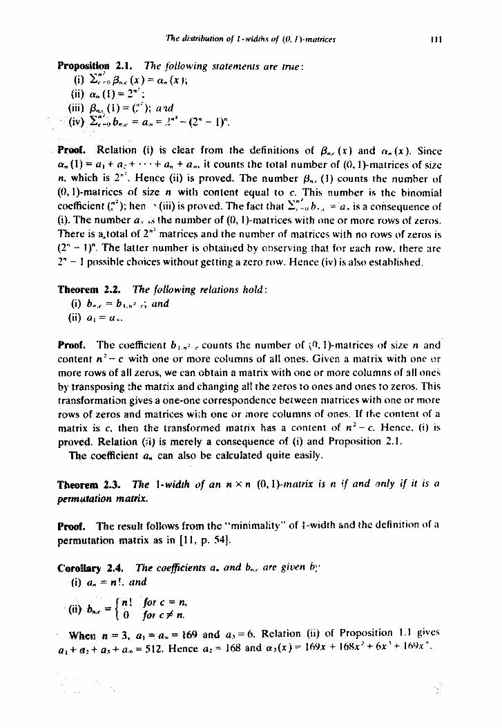
Proposition 2.1. The fotbliuwing StutenzentS are true: (i) Z$ pnr (x) = CY, (x j;

(ii} rw, (I) = 2”‘;

(iii) &, (I) = (,“‘); clrd

(iv) I&, b,,, = a, = 1”” - (2” - 1)“.

Proof. Relation (i) is clear from the definitions of P,,< (x) and IY, (x). Since

a, (1) = cl1 + cl> + * * * -f- a, + a,, it counts the total number of (0, l)-matrices of size

II, which is 2”‘. Hence {ii) is proved. The number &, (1) counts the number of

(O,l)-matrices of size n with content equal to c. This number is the binomial

coefficient fz’); hen * (iii) is proved. The fact that x:t,, b,., = a I is a caisequence of

(i). The number a, Ia the number of (0, I)-matrices with one or more rows of zeros.

There is a,total of 2”’ matrices and the number of matrices with no rows of zeros is

(2” - 1)“. The latter number is obtained by o!lscrving that for each row, there are

2” - 1 possible choices without getting a zero row. F-fence (iv) is also established.

Theorem 2.2. The following relations hold: (i) b,., = bl.“2 C; and

(ii) ul = a,.

Proof. The coefficientt bl.nl.C counts the number of i0, I)-matrices of size u and

content n’ - c with one or more colllmns of all ones. Given a matrix with one M

more rows of all zeros, we can obtain a matrix with one or more columns of a11 ones

by transposing the matrix and changing ah rhe zeros to ones and ones to zeros. This

transformation gives a one-one sorrespondence between matrices with one or more

rows of zeros and matrices wi;h one or more columns of ones. If the content of a

matrix is c, then the transformed matrix has a content of n2 - c. Hence, (i) is

proved. Relation (ii) is merely a consequence of (i) and Proposition 2.1.

The coefficient an can also be calculated quite easily.

Theorem 2.3. Tt;re permutation matrix.

J- wirfth of an n x n (0,l )-matrix is E if and only if it is a

Proof. The resutt follows from the “minimality” of i-width and the definition of a

permutation matrix as rn (11, p. 541.

c’or0alaq ~4. The ccleffieients a, (i) an = n !, and

(ii) b,, = n! furc=n, 0 forcfn.

When n = 3, ar = a, = 169 and

Q~ -t LI.! + LS> + a, = 512. Hence a2 =

and b,, are given b:?

aa = 6. Relation

168 and cu,(xj=

(ii) of Proposition 1 .I gives

169x + 16Xx’+6x’+ IWX’.

112 c. W.U. l..am

We succeed in finding ai because we can find the values of ~1~ and n=. The

corresponding cocffjcients b,., and B,.,, can aiso be calculated, We wilf define

g(n, k. :. r) as the number of k X n (0. I)-matrices with content c’ and having exactly r rows of zeros.

Propsitioll 2.5. The coeficiertr PL., cnn bri, expressed as

L = 2 g(n, k,c,r). v-1

The values g(n, k, c, r) can Cle cafcufated recursive&.

Algorithm 2.6. The value of g (n, k, c, r) cm be calcubted recursir ely as follows : (i) for c 20 and k >rsO,

g(n,k,c,r)=g(n,k - l,c.r- l)+

(ii)for r C 0,

g(n, k, c, I) = 0;

(iii)_$r c = 0,

g(n,k,O,r)= 0 if k # r, 1 ifk=r;

(iv) for k = r,

gOt,kc, k)= 0 ifc#O. 1 ifc=O.

Remarks on Algorithm 2.6. Steps (ii), (iii) and (iv) are used to catculnte the value of the function g when the recursion has reduced it to a case simple enaugh to calcujate. Step (ii) says that tttere exids no matrix with a negative number of +oWS of zerm. S%ep (Si) says ttrat !he only possible matrix with a content of 0 is the zero matrix. Step (iv) says that the zero matrix must have content 0.

Step (i) is the main recursion step. It evaluates g (n, k, c, I) by separately counting two kinds of matrices: the first kind in which the first row of the matrix is filled with ZCTUS 7~4 GW s~3nd kind in wkir% IIw first row has one or more nonzefo entries. If the first row is compieteiy zero, then one only needs to count the number of fAi - i>X n _m~3ti~~~ G.& .wzw~~~ F - 2 r-f of zerm. 2t &%T firr*t ~5 & I-R* coq~leiel~ zero, then one or more of its positions are ones. If there are i l’s in the fk TOW. WXI ‘there are F) choices Ior the first row. The cantent of the remaining

(k-l),4nsubmatrixisc-’ z. Hence, each of the (r ! choices for the first row gives rise tog(n, k - i,, - i, r) matrices. The summation,pes osly up to the minimum of n and c because there can ,at must be c I ‘s- ia the first rkw if x < n.

If r = 0 when step (i) is applied, then v&e. aill get a c~s&‘wbe~e the stew r = - 1.

&)wcvpr, step (iii) tclfs us that rhe value of g(n, k, e, -- 1) = 0.

We are assuming that n, k, c, and r are all notI-negative intepcis to start with. ‘rho

algorithm is to apply step(i) repeatedly. Every time step (i) is applied. the value of k

decreases by I. Hence the recursion of step {i) is finite. When cone LR more of the

conditions in step (i) fails. one of the other steps will be used. It is a simple mat!cr to

check that in all possible cases where step (i) cannot hc rrppfied. the other creps will

supply the correct value of g(n, k: c, r).

Using these recursive calculations and Propositicrn 2.5, the values of b,.,. can he found. Relation (iv) of Proposition 2.1 provides an independent check of the results. Fr<)m the values of b,.,. we can calculate the values of b,,, using (i) OF

Therjrem 2.2. Some of these values can be double checked because we can find the

polynomial & (x) explicitly for sme ~3lues of c.

Proof. Skce there are less than pt I’s in the matrix. one of the rOw sums must be

equal tu 0. Hence the l-width of the matrices with c < n is equal to =c. Thus the

theorem folbws from (iii) of Proposition 2.1.

Using (i) of Theorem 2.2 we obtain the next corollary.

?z2 - II + I s c si n’. WC: can also calculate the coefficients b,,, and h, ., for any c.

The following resutts give some con&Cons which imply b,., = 0. In particuiar we can

tind&,.,(x)f~r n’--2n<cGn’-n.

Lemn~ 2.9. Let s be fhe maximum column mm of n (3, I)-tmtrix A. lf w (A ) 4 x,

rhen w(A)G 1 +(n -s).

Proof. Since w(A)< m, there exists a choice of columns which will cover all the

raws. If we chmse the column whose column sum is s, then there are only n - s

POWS left unc~ere#. Since there is a feasible cover, there exists a set of at nm?

n-. s c~lun~ns which will cover the above n - s rows. Hence we have constructed :d

cover with 1 + fr - S) columns. Since w(A) is the minimum size of any cover. the,

resuk frsllows.

Theorem 2.10. tt~r c be the content of a (0. I)-murris A of order II. If w (,4 ) -C x.

them

w(A)zX+(n”-c)lra.

Pr&. Let .s be the maximum c&umn sum, Then we have ns z c, wnich impiies

114 c. WM. Lum

rhat s B c/n. Together with Lemma i1.0, wc have

w(A)G I+ (M - c/n).

which implies that

Corollary 2.11. If~~ii>+((n2-C)/H, thenb,,=O.

Praclf. The coefficient b,., counts the number of (0, l)-matrices with content i: and I-width i. However. Theorem 2.10 implies that all matrices with content c have I-width less than the value of i :‘i the corollary. Hence the corollary is proved.

In particular. if c is in the range n’- 2n < c d rz’- n, then I f (n’- c)/n =C 3. Hence for c in that range and i in the range 3 d i G n, we have bi,, = 0. Thus the only nonzero coefficients of &C (x) are b,.,, bj,, and b,.,. The values of b,,=, b,,= and 6t.c -I- bz.‘ t ba,, a& known. tie:~~ & can be calculated..

Wnfortunately, this kind of ana!jsis cannot give us all the necessary information to calculate the distribution of l-widths for (0, 1)-matrices of order n 2 4. The next section wilf develop a method of generating and counting all the remaining matrices.

3. A normalization process

The number of (0, I)-matrices of order n increases very rapidly with n. In order to find the distribution of l-widths for matrices of a reasonably high order, we must find a way of obtaining the distribution without actualJy geuerating every single matrix. Fortunately, the l-width of a ma:rix is unchanged under arbitrary row and column permutations. Hence, starting from one matrix A, we can construct many others with the same width by taking all possible row and column permutations on A. Thus, ci’ery matrix generates a set of matrices. The size of this set can be counted easily. We will call such a set a~3 mbit. Our general scheme is to generate oni! one matrix for each orbit until alI the possible orbits are exhausted. We wilt lir\r introduce some terminology from group theory.

IX? Mm denote the set of all n x n (0, t)-matrices, and let S, be the group of all 11 4 n permutation matrices under matrix multiplication. It is a simple matter to see that the set of permutation matrices does form a group and that this group is isrjmorphic to the symmetric group on n letters. The symbols P and Q will ‘denote permutation matrices. Let G be the group obtained by taking the direct product of ‘- with S,. The elements of G are written as an ordered pair (P, 0). We now define ii mtion of G cJn M, by letting (P, 0,) E G map A E Mm to PAQ E Mm under the

The set A” is called the or&r of A. The sfr~bilizer of A. C;,,. is defined b!

G,, = {(I’, Q)E I;: ?AcS = A}.

If PAQ = A, then we say th;tt (f, 0) fixes A. A well-known result in group theor>

[I, p. Sj is that

(1)

The size of G is known to be (n!)‘. Thus. in order to calculate the size of the orbit

A ‘I, we will calculate the size of the stabi!izer G, . Normally, it is ea~icr to calc’ul.~tc

the size of the stabilizer of a matrix than the size of its orbit.

WC still have the problem of generating one and exactly one matrix for every

orbit. We will impose an ordering on the matrices. For each orbit. we will then

generate the matrix with the highest ordering. Our ordering is obtained by first

ordering ihe row sums. then the column sums, and then the row vectors themselves.

The ordering is chosen in this manner because they arc suitable for computational

purposes. To be exact about the ordering, Ip_t us give the following dcf,nitions.

Let A be a (0, I)-matrix of order m. Let the sum of row i of A be denoted by r, ’

and let the sum of cokmn j of A Ire denoted by s,. We call the vector

R = (rt, rz, . . ., r, ) the row sum uecmr and th,o vector S = cs,, s2,. . . . s, ) the collcmn

SUM uecfor of A. We say that R is monorl>ne provided r, 3 rZ b - . . 2 r,. and a

simikr definition holds Eoor S. We Let E? be another (0. ’ ‘j-matrix of order n with row

sum vector L; = (u,, u2,. . ., u,, ) and column sum veriot V = (u,, vZ,. . ., u, ).

Tocompa ; the two matrices A and B, we first cnnpare the row sums of A and

B. If for some i G n, 9 > u, and r) 57 rc, for i .C i, then we say A > R. If the row sums

are all equal, then we compare the column sums. If s, > v, and s, = v, for j < i. then

we say A > 8. $f b& tie TOW sums aand cotirrm sum% are rr@, then WP rnmpr t‘

the rows of A and B, starting from the first row. For each row we compare the

entrie5 starting from the left, If dl thy rows are equal, then A and I3 are the San?<.

Q_the~.~&e 2ye tiwrJ. &efiz~ ~&&RI 1~ &~ich ,A and B are &Bere~~c. Jf .A ha-s a 3 and

B a Q in that position, then we say that A > B. We write A 3 R for A > 3 ()r

A T= B.

116 C. W.H. Lam

orbit, we can calculate a few more coefkients of the p-polynomials. The remainder of this section illustrates one of these results.

Theorem 3.1. Let A be a (0. l)-marrix of order n with contenf c = n2 - (w - l)n

and width w satisfying n 2 w > 3. Then A can be normalized to a matrix of the form shown in Fig. 1, where d,.Ld2+.,.+dW = n, d,adzr***Bdd, 21, and J is the

(n - w ) X n matrix of all 1-s.

Proof. First of all we will show that the column sums of A are ail equal to

r -- .___-

I 1 . . . T Il.. .l

J

i il. . .1

t n-w

+d,--- d2-+ +-d,-+ Fig. I.

II w + I. Sincc c = n2-- (w - E)n, the average column sum is n - w + 1. If the \.trlumn sums arc not all qu;d to n - w + 1, then there exists a column sum Si which is greater than n - w f 1. Ltimma 2.9 implies that the width of A is strictly less than I + u - (n - w f 1) = w, which contradicts the assumption of the theorem.

Since w s n, a minimum cover exists. Next we wil! prove that the submatrix obtained by taking the columns in a minimum cove: can be periinuted into a matrix with a J matrix of order (n - w) x w a? the top and an identity matrix of order w a? ahe bottom {as illustrated in Fig. 2). We first observe ?lr# every column in such a %uhma?rix is c:ssen?ial, meaning that if we leave it out, ?he~ ode or more rows will be uncovered. Vow, we permute the rows until all ?l&tn - w -t 1) l’s of the first column are n the top part. Ftlrthermore, one of these l’s must be in a row with all IIS remaining positions being O’s, because the cofumn is essential. We move this row 10 the (fi - w + 11th row. Now, there remain w - 1 uncovered rows and w - 1 ti%scntiaI columns. Hence each of .the remaining columns must cover one and exactly one of the remaining uncoverkd JQWS, He&e. the bottom w rows of the aubmatrix can be permuted into an i&r&y matrix. However, .&cc: each column ’

has column sum n - w + 1, each of the top n - w raws.must be fiBed--with 4 $3. I-c? us permute the originaf matrix with the permutations that changed the

‘,‘. ., .

The distrihurion of 1 -widths of (0. I )-nrurrices 117

previous submatrix to the one shown in Fig. 2. We will nov* show that every

remaining cdumn rnrrti be cq’ua~ In one of thr columns in Fig. 2. R&e an): t0f lfie

remaining columns. Since its column sum is n - w -t- I. there mwi be at least one I

in the bottom w rows. We claim that the number is exactly ane. If there were two or

mace I’s in the bottom w MWS, then we can construct a caver with less than w

column:,. We start with the set of columns in the minimal cover used topivc the

submatrix. Since we assume that our extra coh~mn has at kast two l’s in the bottom

w rows. it can replace two columns of the minimal cover and still cover the hc;ttom

W KcnVs. Sk&e- W a 3, ‘rheR? ex&s stilf a C-C~hmrc in rhe <?rigim~ minima> ix-ye-7 which

w2< ceve4: @t-e k&p R - w -xwa, Tkw we .!wte d cc..t<c w:&h <R&~ +? - .? cw$=mm.

which is a conlaadiclion. Hence every remaming co‘iumn ‘n3s exa& tn -- IV) I’s in

the top n -- w rows and one 1 in the bottom w rows. 1 hsrclorc, it is equal to one of

the columns in Fig, 2. Thus the whole matrix can be pcrmulrd into the form shown

in Fig. 1. Further row and column permutations will normalize it so that the row

sum vectors anti column sum vectors are monotone. The condition that n, +- d, +-

- - . -t- d,, = n merely says that the number of columns is II. The condition that rl, --?

d 2-I = . + . a d, a f says that the matrix is normalized and that evcrv row is covered.

J’he condition that w 3 3 is necessary because the 3 X 3 matrix with O’S down the

diagonal and l’s everywhere else cannot be normalized to the form given in Fig. 1.

CuruHary 2, I I stales thal b,., = 0 Inr c > n L - { w - 1 )a Thekxem 3. \ essa>tiaU:,

characterizes the matrices with c = n’ - (w - 1)n. It i. s now a simple matrer to find

the size of t&e orbit for each of the normzdizqd matrices with width w and conrent

C”# ‘--(w - 1)n. Hence we can calculate ihe corresponding b,.,. F&t of &I+ given a vector 0 = (dl, . . , , da ) and an II ?= d, for all i, we define the

multQ&ity vector E = [elr . . ., e, ) where C, denollcs the number of fins~s ihat 1

b&ngs IO the vector D. FIT example, ihc multi@iciiy vector Bar 0 = (2, I, 1) and n = 3 is E = (2,l.O). We also use the standard definition that O! = 1.

wkre the summalionis r&n over aN possible d, ‘s satisfying cl, + cl2 + * l +d, = n and d, a d2 3 - - - 2 d, a 1, and the vector (P,,., ., e, ) is the multiplicity uecfor a/

id 1. e . ., d, ).

pw. By Theorem 3.1, every matrix with c = nz - (w “- 1)n and n 3 w b II can kc normalized to the form shown in Fig. 1, Hence ii is in t bne of the orbits generated by matrices of that particular form. Moreover, if we Lonsidcr atl possible d,‘s

rhc conditions of this theorem, then WC would have considt,rcd all the ortrrfs. l A’c Irlrti count the size of each of these orbits. We do ir by counting the size of the

sta:‘lifizcrs for each matrix of the form shown in Fig. 1. The (n - w)! permutations that f?Cr‘fnUi~ the first (n - w) rows fix the mtrix. The same is true for the d,t ~rmuiaiions that permute the first dl columns, the dtl permutations that permute the next dr culumna, and so on. Moreover, if some of the d$‘s ate the same, we can

rmuic whole blocks of columns with equal d,‘s among themselves while at the *aR?C Gm ~~mu&rg the cuff~sf?~&fflg ro(vs. T?ris last kirrd 0C permuCaIion explains the terms e,! * - - Q .!. These are all the possible permutations that fix a matrix of the b-m shown ia Fig. 2. The order of 0, the group of row and cofumn ~rmuiaiions is (II!>“. Hence the size of the orbit is given by the individual terms of the summation in Theorem 3.2, and the theorem Es proved.

Ar a simple illustration, let us calcufaie the co&Cent h,,zr for n = 6. The f~:rrritions of 6 satisfying the conditions of Theorem 3.2 are 4 -+ 1 t 1, 3 t 2 + I and 2 4 2 4. 2. 79rcir multiplicity vectors are (2,C’I,O, l,O,O), (1,1,1,0,0,0) and 6% X0, (1. Rff) respeciivefy. It is now simple to evaluate bW., according to the fr*rnltifa of Theorem 3.2 and find that b,., = 10800 for n = 6.

4. The avci*age l-width

lfeftsrc WC can discuss what the average l-width is for (0, f)-matrices of order n, avc to decide what to do with matrices A having width ~0, For the purpose of

~-~~~~jai;n~ the avera$e I-width, it is reaso~ahk toh BSSU~XZ that w (A) is a I%% t>fl all. this a~uInpcjon will make the ~~~~~~~~:~n~te numbers %xondIy, we may de&de

w as many columns as po&bk to ,tiy to cove a ma%@% that ‘has MB ‘f+~&#e ~~~~~~. ‘f~~~~. the average l-width &, is defined a8

Tut& 2. Average I-wictrh ci, for ‘5 6 ,I, rtrultdcd 10 4 drcinul places. .-..-s-.w._L-_r_l”_MyI -._^-I CI_-..-.I.._I.I--.-_- _.-_ __-._ ._.._. ___ ._.^_I.._ _

i?, = 1.0 ‘ti .* 2.2733 ii, L-i I .%a t;, .Lz 2.3fwq ii* a ml17 ir,, n Z..w.s~

~~-1.~----I--l--l~~--~~.~“~.--“~~.-I~-.I--.___-_C -,- _.- _.__“_ ___ _~__~~_~___.~~_~~_~_~___

From the proof of Theorem 2.2, we have obtained pairs of matrices the sum of

whose widths is n + 1. Let us iormt;hze the method by giving some dctinitions.

Let A he a (0, I)-matrix of order n. WC Set A ’ denote the matrix ohtaincd hy

transposing A and changing ail the zeros to ones and ones to zeros. WI: let C’

denote the conten; of A *. Ctcarly c * = n’- c. The width of the m;ltriccs A and A *

arc closc~y rclarerf.

Theorem 4.1. 7%e widths of A and A * .salis[y

w(A) -+ w(A *) G n + 2.

Equality halds if mtd orrly if :ither A or A * is 0 permtrttitin~~ nrcrtrix.

(3)

Proof. If either A or A * has no fcasihle cover, then (3) follows from the proof of

Tncarern 2.2. In ‘iacl wlAj ‘r w\A*j = n + ‘I ‘rn Ik’ls ca5c. So, wc can iw~~nic t'niil

both w(A) und w(A *) are finite in the remainder of this proof.

From Theorem 2.10, we have

w(A*)d 1 +(n’- c*)/n. (5)

t C. W.H. Lam

ctmaidcr the case when both tv(h ) C 3 and w(,A *) < 3. ff one of the Iwo widths is 1, then w(A) + w(A “) 3 n + 1 from the proof of Thearern 2.2. Thus, the only

possibility left is that w(A) = w(A “) = 2. However, in this case, we have n ,f 2 -

w(A ) + WJ[A ‘) =a 4 which implies Ihat n = 2. Hcncc, Theorem 2.3 implies that buth

permutation matrices.

enerality, we assume that w(A) 2 3. Then the matrix A can be

n~~rrn~li~~d to farm shown in Fig. 1. Therefore, it is clear that w(A *) = 2.

nce w(A ) + w(A *) = n + 2 implies that w(A ) = n. Again, Theorem 2.3 implies

t A is a pcrmutatia,n matrix, and the theorem is proved.

up the values of 6. in Table 2, we see :hat the corollary is true

assume n > 6 in the rest of the: proof.

‘~~~~r~rn 4-1 establishes that except for the n! pairs of matrices cjbtained from

the permurstion matrices, all o:her matrices can be paked up to give a tofal width

cd lcsis than or equal to n + 1. We now show that there exist mare than n! pairs

whr total width is strictly less thain n + 1. Consider the matrix A shown in Fig. 3.

Fig. 3.

Hcrc .I -- I denotes the matrix of order n - I with O’s in the nvtin diqpnal and I’s etcrywhere efse. It is clear that w(A ) = 3 and w (A *) = 2. Since tt b 6,

wI(A ) + w(A *) = 5 -C n + 1. The size of the stabilizer of A is (n - I)!. Wence the

$ize of the orbit A ” is n (n ! ). Thus, the orbit A a gives rise to more than n ! pairs ~th total width strictly less than n + 1 and the theorem is proved.

Section 2, we can easily ~&x~iatc the coetioicnts b,., and h,,, for ai1 C’S, as well as

the /3-polynomials &,< (x) for c S= n and c .r tt I - 2n. Thus, to procrtod further WC

have to generate and count the mstrices whose cc~ntent c satisfies tt ST c 5: tl* zrl

and whose width w satisfies 1 c w G II.

Et~t t%cfl c W+Z generate &l the monotone row sum vectors whose row sums arc

nonzero, l%cy are the ordered partitions of c into n parts. Next, we generate the

cohm~n sum vectors, which are the ordered partittons of c into n or fewer parts. ,411

the parts have to be less than n. For each pair of row sum and column sum vectors.

we generate all the normalized matrices. The actual method is 10 start from the rtrp left comer and to put in I’s where appropriate. The process of determining whctkr

a matrix is normalized is combined with the process to calculate its st;lhilizor.

Let us cali the original matrix A and WC let R denote the matrix obtained after ,I

column permutation which pcrmutcs cl)lumns with the \ame colum!l sum. If a row

permutation of R gives a matrix which is greater than A. then A is not normalkcd.

7’0 simplify this process. WC‘ regard every 1’0% as a b&tar> number called its TOW

oalue. Among the rows with the same TOW sum, a normalized matrix will have its

row values in decreasing order. The matrix A is gcneratcd with this properly. We

sort the row values of B among rows with the same row sums. The matrix R can ht~

permuted to A by row permutations if and only if the sorted row values of B are

the same as those of A. The numbeqof such permutations equals the product of the

factorials of the entries in the multi@icity vector of the row values. The method of I

using row values speeds up the calcu!ation considerably.

For each normalized matrix, WC calculate its l-width. With this method. we

determine all the P-polynomials. The u-polynomials are obtained using (i) of

Proposition 2.1. The cu.polynomials for n G b are !isted in Table I. A list of the

@-polynomiak fo; 2 G n 6 6 is available frorl the author.

111 N. k%ggs. finite Ciroupv of Automorphioms. London Math. Sot. Lecture Notes Scric$b (ramhrldpc Univcrt4ty Frer~. Oxford, 1071).

[Z] S.A. &ok, The complexity of theorem-proving procedure. rn: Proc. Third Annu;rl ;Y(‘hl Symposium on the Theory of Computing. Shaker Heights. OH flY71) 151-158.

f:.!] J. f?dmonL, Paths. trees and flowers. Can: J. Math. 17 (1965) 449-467. [4f L).ff. Fulkcnc~n and HJ. Wystrr, Widths and ht4phts of (0, I)-matrices. Can. J. Math. 13 (i.;c,l)

23%2!3. ,. .i

151 l3.R. Fulkc:rioQn and M.J. Ryser, Multiplicities and minimal widths for (0. I )-matnces. Can J Mrrth 14 (1962) 4!%-“508.

f?‘] J.R. #%x&mm artd R.A. Dean, Tttc t-width of (C I)-matrices having constant row sum 3. J Combinararial Titeary Ib (19‘74) .355-370.

($j R.M, f&p, Reducibility among combinatorial prohicms, in: Compiexiry taf Computer C’clrnp~~t;~ ritmtnu (Plrnum Press, New York, l!W 8%103.

822 c. W.H. imn

{q R.Z. Norsmart and MO. Rabin, An algorithm for a minimum cover of a graph, Proc. Am. Math. !bc. 10 (1959) 315-319.

(la) D.K. Ray-Chaudhuri, An algorithm for a minimum cover of au abstract complex, Can. J. Math. 15 (1963) I l-24.

(Ii] HJ. Rywr, Combinatorial Mathematics, Carus Monograph No. I4 (Wi&, New York, 1%3). [l2l H.&l. SalI& and R.D. Koncal, Se1 covering by an all inieg& slgonshm: cot&rational experie&,

lltl depth of a class of (0, I)-matrices, Math. USSR-Sb. 4 (1968) 3-12.