the differential rates of exclusive charmless semileptonic ... · the differential rates of...

THE DIFFERENTIAL RATES OF EXCLUSIVE

CHARMLESS SEMILEPTONIC B MESON DECAY

A Dissertation

Presented to the Faculty of the Graduate School

of Cornell University

in Partial Fulfillment of the Requirements for the Degree of

Doctor of Philosophy

by

Matthew Randall Shepherd

August 2005

THE DIFFERENTIAL RATES OF EXCLUSIVE CHARMLESS

SEMILEPTONIC B MESON DECAY

Matthew Randall Shepherd, Ph.D.

Cornell University 2005

The rates of exclusive charmless semleptonic B meson decay provide experimental

input necessary to extract the magnitude of Cabibbo-Kobayashi-Maskawa quark

mixing matrix element Vub, which can be used to search for physics beyond the

Standard Model through precision tests of the parameters of the weak interac-

tion. Using the CLEO detector at the Cornell Electron Storage Ring, we analyze

30.8 million B meson decays to measure the rates of decay for B0 → π−`+ν and

B0 → ρ−`+ν. The measurement is made in bins of the lepton decay angle in

the W helicity frame and the four-momentum transfer to the virtual W , q2, to

minimize dependance on the theoretical form factors that govern the decay dy-

namics. The total rates are B (B0 → π−`+ν) = (1.32± 0.15± 0.11± 0.02)× 10−4

and B (B0 → ρ−`+ν) = (2.73± 0.36± 0.32± 0.04) × 10−4 where the errors are

statistical, experimental systematic, and theoretical systematic respectively.

BIOGRAPHICAL SKETCH

Matthew was born on August 23, 1978 in Evansville, Indiana. He attended

William Henry Harrison High School where his interest in physics was first kindled

by Mike Kelly, his high school physics teacher. With visions of medical school

in the future, he choose to pursue a degree in physics. In the fall of 1996 he

headed just north of his hometown to begin his undergraduate studies at Indiana

University in Bloomington.

The next four years at Indiana University forever changed his life in two ways.

Most notably he met his future wife, Catherine Magee, then a ballet student at

the university. In addition, through several years of work in the research group of

Alex Dzierba, he realized his true love of physics and decided to pursue a Ph.D. in

experimental elementary particle physics.

After receiving bachelors degrees in physics and mathematics from Indiana

University in 2000, Matthew moved to Ithaca, New York to begin to embark on

his Ph.D. at Cornell University. In early 2003 he began his dissertation research

on exclusive charmless semileptonic B decays with Professor Lawrence Gibbons

and, later that year, received an M.S. degree in physics.

In the summer of 2003 he and Catherine were married. They will be returning to

Bloomington in the fall of 2005 where Matthew will begin an assistant professorship

at his alma mater.

iii

ACKNOWLEDGEMENTS

I would first like to thank my advisor, Lawrence Gibbons, for his guidance and

patience throughout my dissertation research. In addition this research would not

be possible without the extensive help of Richard Gray and those who have been

involved in this analysis over the years: Veronique, Andreas, Tom, Nadia, Ed, and

others.

I want to acknowledge those who inspired me to pursue physics as a career. My

high school teacher, Mike Kelly, responsible for my choice of physics as a field of

study, and it was Alex Dzierba who lead me to discover my love for experimental

research work. Without them I am not sure what career path I would have chosen,

but I am certain that I would not be having as much fun as I am now.

I am grateful to Tom Meyer for enriching my experience at Cornell. As a fellow

student and colleague Tom was a wonderful mentor. In my early years, he taught

me almost everything I know about the inner workings of the CLEO detector. Our

parallel dissertation topics also provided another opportunity for me to learn from

Tom’s experience. I will certainly miss our fun and productive discussions.

I would like to thank my fellow grad students: Rich, Dan, Mark, Greg, and

others who were in our entering class. We stuck together and supported each other

throughout a torturous year graduate coursework. Throughout the years my wife

and I have enjoyed the friendship of Pete, Adie, Christine, Tom and Janis. I thank

them for making the experience in Ithaca a fun one. I would also like to thank all

of those who made Wilson Lab such an exciting place to work, including my office

mates past and present: Alan, Jean, and Dan.

Finally I would like to thank my wife, Katie. Her continued love and support

has allowed me to be productive as a student and researcher.

iv

TABLE OF CONTENTS

Biographical Sketch . . . . . . . . . . . . . . . . . . . . . . . . . . . . . . iiiAcknowledgements . . . . . . . . . . . . . . . . . . . . . . . . . . . . . . ivTable of Contents . . . . . . . . . . . . . . . . . . . . . . . . . . . . . . . vList of Tables . . . . . . . . . . . . . . . . . . . . . . . . . . . . . . . . . viiiList of Figures . . . . . . . . . . . . . . . . . . . . . . . . . . . . . . . . . ix

1 Motivation 11.1 Discovery of CP Violation . . . . . . . . . . . . . . . . . . . . . . . 11.2 CP Violation in the Standard Model . . . . . . . . . . . . . . . . . 21.3 Connecting B → Xu`ν with CP Violation . . . . . . . . . . . . . . 8

2 Theoretical Background 102.1 Decay Kinematics . . . . . . . . . . . . . . . . . . . . . . . . . . . . 102.2 The Decay Form Factors . . . . . . . . . . . . . . . . . . . . . . . . 13

2.2.1 Calculation Techniques . . . . . . . . . . . . . . . . . . . . . 142.2.2 General Form Factor Behavior . . . . . . . . . . . . . . . . . 15

3 Experimental Apparatus 183.1 The Cornell Electron Storage Ring . . . . . . . . . . . . . . . . . . 183.2 The CLEO Detector . . . . . . . . . . . . . . . . . . . . . . . . . . 19

3.2.1 Charged Particle Tracking . . . . . . . . . . . . . . . . . . . 213.2.2 Particle Identification . . . . . . . . . . . . . . . . . . . . . . 223.2.3 Calorimetry . . . . . . . . . . . . . . . . . . . . . . . . . . . 243.2.4 Muon Detection . . . . . . . . . . . . . . . . . . . . . . . . . 25

3.3 Data Summary . . . . . . . . . . . . . . . . . . . . . . . . . . . . . 25

4 Experimental Technique 284.1 The Fundamental Objects: Tracks and Showers . . . . . . . . . . . 29

4.1.1 Tracks . . . . . . . . . . . . . . . . . . . . . . . . . . . . . . 304.1.2 Showers . . . . . . . . . . . . . . . . . . . . . . . . . . . . . 314.1.3 K0

S’s and other “Vees” . . . . . . . . . . . . . . . . . . . . . 324.2 Particle Identification . . . . . . . . . . . . . . . . . . . . . . . . . . 35

4.2.1 Lepton Identification . . . . . . . . . . . . . . . . . . . . . . 354.2.2 Hadron Identification . . . . . . . . . . . . . . . . . . . . . . 424.2.3 Monte Carlo Considerations . . . . . . . . . . . . . . . . . . 44

4.3 Signal Hadron Reconstruction . . . . . . . . . . . . . . . . . . . . . 464.4 Final Candidate Reconstruction . . . . . . . . . . . . . . . . . . . . 484.5 Figures of Merit . . . . . . . . . . . . . . . . . . . . . . . . . . . . . 53

4.5.1 A Basic Figure of Merit . . . . . . . . . . . . . . . . . . . . 534.5.2 A Figure of Merit for a Rate Measurement . . . . . . . . . . 55

4.6 Continuum Suppression . . . . . . . . . . . . . . . . . . . . . . . . 574.6.1 Event Shape Variables . . . . . . . . . . . . . . . . . . . . . 584.6.2 Constructing a Fisher Discriminant . . . . . . . . . . . . . . 60

v

4.6.3 Cut Implementation and Optimization . . . . . . . . . . . . 624.7 b→ c Background . . . . . . . . . . . . . . . . . . . . . . . . . . . . 64

4.7.1 Lepton Momentum Requirement . . . . . . . . . . . . . . . 644.7.2 Track Multiplicity Criteria . . . . . . . . . . . . . . . . . . . 654.7.3 B → J/ψK0

L . . . . . . . . . . . . . . . . . . . . . . . . . . . 664.8 Neutrino Quality Cuts . . . . . . . . . . . . . . . . . . . . . . . . . 68

4.8.1 The V Cut . . . . . . . . . . . . . . . . . . . . . . . . . . . 684.8.2 Net Charge . . . . . . . . . . . . . . . . . . . . . . . . . . . 714.8.3 Additional Cuts . . . . . . . . . . . . . . . . . . . . . . . . . 71

4.9 Selecting the Best Candidate . . . . . . . . . . . . . . . . . . . . . . 724.9.1 Combinatoric Considerations . . . . . . . . . . . . . . . . . . 734.9.2 Signal Efficiencies . . . . . . . . . . . . . . . . . . . . . . . . 75

5 Fitting the Data 775.1 Binning . . . . . . . . . . . . . . . . . . . . . . . . . . . . . . . . . 77

5.1.1 The Fit Plane . . . . . . . . . . . . . . . . . . . . . . . . . . 785.1.2 q2 and cos θW` Binning . . . . . . . . . . . . . . . . . . . . . 805.1.3 Decay Mode Binning . . . . . . . . . . . . . . . . . . . . . . 835.1.4 Net Charge Binning . . . . . . . . . . . . . . . . . . . . . . 845.1.5 Bin Summary . . . . . . . . . . . . . . . . . . . . . . . . . . 84

5.2 Weights and Strengths . . . . . . . . . . . . . . . . . . . . . . . . . 855.3 Fit Components and Parameters . . . . . . . . . . . . . . . . . . . . 86

5.3.1 Generic b→ c Decays . . . . . . . . . . . . . . . . . . . . . . 865.3.2 Continuum Background . . . . . . . . . . . . . . . . . . . . 885.3.3 Fake Signal Leptons . . . . . . . . . . . . . . . . . . . . . . 915.3.4 Signal B → Xu`ν Decays . . . . . . . . . . . . . . . . . . . . 935.3.5 Other B → Xu`ν Decays . . . . . . . . . . . . . . . . . . . . 955.3.6 Constraints Between Data Sets . . . . . . . . . . . . . . . . 965.3.7 Parameter Summary . . . . . . . . . . . . . . . . . . . . . . 96

5.4 Performing the Fit . . . . . . . . . . . . . . . . . . . . . . . . . . . 985.4.1 A Binned Likelihood Fit . . . . . . . . . . . . . . . . . . . . 985.4.2 Managing Finite Fit Component Statistics . . . . . . . . . . 99

5.5 Fit Results . . . . . . . . . . . . . . . . . . . . . . . . . . . . . . . . 101

6 Systematic Uncertainties 1116.1 Systematic Uncertainties in Neutrino Reconstruction . . . . . . . . 112

6.1.1 Track Efficiency and Resolution . . . . . . . . . . . . . . . . 1136.1.2 Shower Efficiency and Resolution . . . . . . . . . . . . . . . 1146.1.3 Splitoff Simulation and Rejection . . . . . . . . . . . . . . . 1146.1.4 Particle Identification . . . . . . . . . . . . . . . . . . . . . . 1156.1.5 K0

L Production and Energy Deposition . . . . . . . . . . . . 1166.1.6 Secondary Lepton Spectrum . . . . . . . . . . . . . . . . . . 117

6.2 Additional Sources of Systematic Error . . . . . . . . . . . . . . . . 1176.2.1 Continuum Suppression . . . . . . . . . . . . . . . . . . . . 117

vi

6.2.2 B → Xc`ν . . . . . . . . . . . . . . . . . . . . . . . . . . . . 1196.2.3 Other B → Xu`ν . . . . . . . . . . . . . . . . . . . . . . . . 1206.2.4 Lepton Identification and Fake Leptons . . . . . . . . . . . . 1206.2.5 π0 Identification . . . . . . . . . . . . . . . . . . . . . . . . . 1226.2.6 Number of Υ → BB Events . . . . . . . . . . . . . . . . . . 1226.2.7 τB+/τB0 and f+−/f00 . . . . . . . . . . . . . . . . . . . . . . 123

6.3 Dependance on Form Factors . . . . . . . . . . . . . . . . . . . . . 1236.3.1 The B → π`ν Form Factor . . . . . . . . . . . . . . . . . . . 1256.3.2 The B → ρ`ν Form Factor . . . . . . . . . . . . . . . . . . . 126

7 Summary and Conclusions 1287.1 Summary of the Rates . . . . . . . . . . . . . . . . . . . . . . . . . 1287.2 Comparison with Other Measurements . . . . . . . . . . . . . . . . 1297.3 Final Thoughts . . . . . . . . . . . . . . . . . . . . . . . . . . . . . 130

A CLEO III Muon Identification Efficiency and Fake Rates 132A.1 Muon Efficiency . . . . . . . . . . . . . . . . . . . . . . . . . . . . . 132

A.1.1 True Muon Sample in Data . . . . . . . . . . . . . . . . . . 132A.1.2 True Muon Sample in Monte Carlo . . . . . . . . . . . . . . 133A.1.3 Divisions Among Run Ranges . . . . . . . . . . . . . . . . . 134A.1.4 Efficiency Comparison . . . . . . . . . . . . . . . . . . . . . 134A.1.5 Efficiency Correction . . . . . . . . . . . . . . . . . . . . . . 137

A.2 Muon Fake Rates . . . . . . . . . . . . . . . . . . . . . . . . . . . . 137A.2.1 π or K Faking µ . . . . . . . . . . . . . . . . . . . . . . . . 138A.2.2 p Faking µ . . . . . . . . . . . . . . . . . . . . . . . . . . . 140

REFERENCES 142

vii

LIST OF TABLES

3.1 Summary of data sets . . . . . . . . . . . . . . . . . . . . . . . . . 26

4.1 A summary of the reconstructed hadron final states. . . . . . . . . 474.2 Summary of track multiplicity cuts . . . . . . . . . . . . . . . . . . 664.3 Values of the V ratio cut for various reconstructed modes . . . . . 704.4 Reconstruction efficiencies for π`ν modes . . . . . . . . . . . . . . 754.5 Reconstruction efficiencies for ρ`ν and ω`ν modes . . . . . . . . . . 764.6 Reconstruction efficiencies for η`ν modes . . . . . . . . . . . . . . . 76

5.1 The binning used in the Mh`ν and ∆E variables. . . . . . . . . . . 795.2 q2 binning for reconstructed π`ν modes . . . . . . . . . . . . . . . 805.3 q2 and cos θWl binning for ρ`ν modes . . . . . . . . . . . . . . . . . 835.4 Summary of fit bins . . . . . . . . . . . . . . . . . . . . . . . . . . 845.5 Summary of fit components and parameters . . . . . . . . . . . . . 975.6 Central values for the branching fractions for B0 → π−`+ν. . . . . 1025.7 Central values for the branching fractions for B0 → ρ−`+ν. . . . . . 103

6.1 Systematic errors associated with neutrino reconstruction . . . . . 1186.2 Complete list of experimental systematic errors . . . . . . . . . . . 1246.3 Systematic errors associated with form factor calculations . . . . . 127

7.1 Summary of branching fractions for B0 → π−`+ν. . . . . . . . . . . 1297.2 Summary of branching fractions for B0 → ρ−`+ν. . . . . . . . . . . 129

viii

LIST OF FIGURES

1.1 Graphical sketch of CP violating mechanism . . . . . . . . . . . . . 51.2 The unitarity triangle . . . . . . . . . . . . . . . . . . . . . . . . . 71.3 Current experimental constraints on the apex of the unitarity triangle 7

2.1 Kinematic variables in B → Xu`ν decay . . . . . . . . . . . . . . . 132.2 The B → π form factor: f+(q2) . . . . . . . . . . . . . . . . . . . . 162.3 The B → ρ form factors . . . . . . . . . . . . . . . . . . . . . . . . 16

3.1 A schematic of the CESR machine. . . . . . . . . . . . . . . . . . . 193.2 A side-view of the CLEO II detector. . . . . . . . . . . . . . . . . . 203.3 A 3D cutaway view of the CLEO III detector. . . . . . . . . . . . . 203.4 Historical integrated luminosity by month . . . . . . . . . . . . . . 27

4.1 A “curler” . . . . . . . . . . . . . . . . . . . . . . . . . . . . . . . 314.2 Typical π+π− invariant mass distribution for K0

S candidates. . . . . 344.3 Typical pdf’s for electron identification variables . . . . . . . . . . 384.4 Electron identification efficiency as a function of momentum . . . . 404.5 Muon identification efficiency as a function of momentum . . . . . 424.6 Missing energy and missing momentum resolution . . . . . . . . . . 494.7

∣∣tcand · tROE

∣∣ for signal and continuum events . . . . . . . . . . . . 594.8 R2 for signal and continuum events . . . . . . . . . . . . . . . . . . 594.9 Reconstructed q2 of B → π`ν candidates in off-resonance data . . . 624.10 Typical performance of continuum supression algorithm . . . . . . 634.11 The spectrum of leptons produced in B decays . . . . . . . . . . . 654.12 Lepton spectra for B → π`ν and B → ρ`ν decays . . . . . . . . . . 664.13 Track multiplicity for signal and background events . . . . . . . . . 674.14 Typcial V cut overlaid on signal and background Monte Carlo . . . 704.15 Tagged efficiency vs. minimum π0 energy cut . . . . . . . . . . . . 74

5.1 Bin selection in the ∆E vs. Mh`ν plane . . . . . . . . . . . . . . . 795.2 The effect of a lepton momentum requirement in the cos θW` vs. q2

plane . . . . . . . . . . . . . . . . . . . . . . . . . . . . . . . . . . 825.3 Illustration of binning in the cos θW` vs. q2 plane . . . . . . . . . . 825.4 Sample “smoothed” continuum background . . . . . . . . . . . . . 905.5 Mh`ν projections of the nominal fit for Q = 0, π`ν modes . . . . . . 1035.6 ∆E projections of the nominal fit for Q = 0, π`ν modes . . . . . . 1045.7 Mh`ν projections of the nominal fit for |Q| = 1, π`ν modes . . . . . 1055.8 ∆E projections of the nominal fit for |Q| = 1, π`ν modes . . . . . 1065.9 Mh`ν projections of the nominal fit for Q = 0, ρ`ν modes . . . . . . 1075.10 ∆E projections of the nominal fit for Q = 0, ρ`ν modes . . . . . . 1085.11 Lepton momentum projections of the nominal fit . . . . . . . . . . 1095.12 cos θWl projection of the nominal fit . . . . . . . . . . . . . . . . . 1105.13 Mππ projection of the nominal fit . . . . . . . . . . . . . . . . . . . 110

ix

6.1 Predictions for the q2 dependance of the B → π`ν rate . . . . . . . 1266.2 Predictions for the q2 and cos θWl dependance of the B → ρ`ν rate 127

7.1 Current world results for B0 → π−`ν and B0 → ρ−`ν branchingfractions. . . . . . . . . . . . . . . . . . . . . . . . . . . . . . . . . 130

A.1 Selection of a pure sample of muons in data . . . . . . . . . . . . . 133A.2 CLEO III muon identification efficiency . . . . . . . . . . . . . . . 135A.3 Comparison of Monte Carlo and data muon identification efficiencies135A.4 Comparison of the effect of the online sparsification bug in Monte

Carlo and data . . . . . . . . . . . . . . . . . . . . . . . . . . . . . 136A.5 Selection of a pure tagged sample of D decays . . . . . . . . . . . . 138A.6 Probabilities as a function of momentum for π and K faking µ . . 139A.7 Selection of a pure proton sample in data using Λ → pπ . . . . . . 141A.8 Probability as a function of momentum for p faking µ . . . . . . . 141

x

Chapter 1

Motivation

One of the most outstanding objectives of modern particle physics is to un-

derstand the mechanism by which the matter-dominated universe that we live in

was created. In 1967 Andrei Sakharov proposed three conditions which were nec-

essary to allow baryogensis in the universe [1]. One of the three conditions can

be elegantly accommodated for with the Standard Model of particle physics: the

existence of CP violation. Is this natural source of CP violation the unique source

of CP violation that Sakharov stated was necessary to produce the universe we

live in? This is precisely the question that motivates this work!

1.1 Discovery of CP Violation

In 1957 Wu et al. experimentally verified that the weak interaction violates

parity (P ) by measuring the direction that electrons were emitted with respect to

the nuclear spin in Cobalt 60 beta-decay [2]. The observation that the electrons

were preferentially emitted in the direction opposite the spin of the nucleus meant

that the process must be parity violating as the nuclear spin direction would remain

unchanged under a parity transformation. In fact we know that the structure of

the weak interaction maximally violates parity. Femi’s traditional four-particle

vertex of the weak interaction was replaced by the weak interaction Hamiltonian:

H =GF√

2

[ψ1γµ (1− γ5)ψ2

] [ψ3γ

µ (1− γ5)ψ4

], (1.1)

where GF is the Fermi coupling constant. Parity violation arises due to the

γµ (1− γ5) or “vector−axial-vector” (V − A) structure of the Hamiltonian. The

1

2

(1− γ5) portion simply projects out the left-handed components of the ψs; there-

fore, by construction only left-handed particles or right-handed anti-particles in-

teract weakly.

One might logically think that applying the parity operator (P ), which changes

“handedness”, followed by the charge conjugation operator (C), which replaces

particles with their anti-particles, would be a symmetry of the weak interaction.

However, in 1964 Cronin and Fitch observed that this so-called CP symmetry

was violated in the weak decays of neutral K mesons [3]. This groundbreaking

observation sparked the search for natural ways to accommodate CP violation

within the emerging Standard Model.

1.2 CP Violation in the Standard Model

To explain strangeness-violating weak decays of K mesons, Cabibbo, in 1963,

proposed that quark eigenstates of the weak interaction were not the same as those

of the strong interaction [4]. At the time, only u, d, and s quarks where known to

exist, and Cabibbo’s solution was that the s and d quarks of the weak interaction

were different than those of the strong interaction. Mathematically: d′

s′

=

cos θC sin θC

− sin θC cos θC

d

s

, (1.2)

where the prime denotes the weak interaction states and θC , the Cabibbo angle,

is the amount the that weak states are rotated from the strong states1. K mesons

are therefore produced and bound through the strong force in states of d and s,

and the subsequent hadrons produced in the decay would contain u and d quarks.

1Experimentally this angle is quite small – about 13

3

However, the intermediate weak decay proceeds through the s′ and d′ states. This

allows s→ d transitions and solves the problem of strangeness violating decays.2

Kobayashi and Maskawa realized that an extension of Cabibbo’s idea could also

elegantly account for CP violation in the Standard Model [5]. They predicted the

existence of an additional two quarks, t and b, to add to the known u, d, and s,

and the proposed c, quarks. Equation 1.2 could then be expanded tod′

s′

b′

=

Vud Vus Vub

Vcd Vcs Vcb

Vtd Vts Vtb

d

s

b

. (1.3)

Now the matrix V , known as the CKM matrix, describes the rotation of the strong

interaction quark eigenstates into the weak interaction eigenstates. The quark-level

weak current in the Hamiltonian is then

J µ = ψuγµ (1− γ5)ψd′ = ψuγ

µ (1− γ5)V ψd, (1.4)

where ψu denote the up-type (u, c, and t) quark and ψd′ and ψd denote the weak

and strong eigenstates of the down-type quark. If we view the quarks as occurring

in three-generations u

d

c

s

t

b

, (1.5)

then the fact that V is not diagonal permits “generation-changing” decays such

as K → π`ν, which is what initially motivated Cabibbo. However, extending the

matrix further to incorporate a third generation of quarks as done by Kobayashi

and Maskawa allows for CP violation.

2It also created a problem in that some decays predicted from Cabibbo’s model werenot observed. Glashow et al. solved this problem with the proprosal of the charm quark,whose presence in the “GIM mechanism” cancels out the unobserved decays. Of coursethe charm quark was later discovered.

4

If there exist strictly three generations of quarks then the CKM matrix must

be a unitary complex rotation matrix. Any arbitrary matrix of such type can be

specified by three angles and a single phase. These four parameters are fundamen-

tal parameters of the Standard Model. The common way [6] to parameterize V in

terms of the three angles, θ12, θ23, and θ13 and the phase δ13 is

V =

c12c13 s12c13 s13e

−iδ13

−s12c23 − c12s23s13eiδ13 c12c23 − s12s23s13e

iδ13 s23c13

s12s23 − c12c23s13eiδ13 −c12s23 − s12c23s13e

iδ13 c23c13

, (1.6)

where the c and s represent cosine and sine of the angles. The subscripts are chosen

to indicate the generation labels. If we “remove” the effects of third generation by

setting θ23 = θ13 = 0 we can recover Cabibbo’s initial matrix (Equation 1.2) and

identify θ12 as θC .

CP operating on a weak current of the form of Equation 1.4 transforms V →

V ∗, thereby flipping the sign of the weak phase. If this phase is the only phase

present in calculation of the matrix element, then the change in sign does not alter

the magnitude of the amplitude. However if additional amplitudes contribute and

they have relative phases which do not change sign under CP , the weak phase can

produce CP violation.

Suppose that in the calculation of some amplitude A two indistinguishable

processes contribute with magnitudes a1 and a2. These processes can be, for

example, tree and penguin diagrams. In the case of some neutral mesons, a1 could

be direct decay to a final state and a2 could be the amplitude to mix first then

decay to the same final state. In any case a1 and a2, being complex amplitudes,

have some relative weak phase δW and some other relative phase, like a strong

5

Figure 1.1: A graphical sketch of how CP is violated using the weak phase δW .Amplitudes a1 and a2 coherently contribute to the full amplitude A. Both a1 anda2 have relative weak phase δW and some other relative phase δS. Under CP theweak phase changes sign causing |A| > |A| and therefore CP violation.

phase, δS. We could then write

A = a1 + a2ei(δS+δW ). (1.7)

Under CP , the sign of the relative weak phase is changed giving

A = a1 + a2ei(δS−δW ). (1.8)

Therefore as long as, δS 6= 0 the amplitudes A and A will not be equal and the

process is therefore CP violating as depicted graphically in Figure 1.1. Kobayashi

and Maskawa proposed that this mechanism was responsible for the observed CP

violation.

Realizing that the magic of the CKM matrix was in the complex phase, and not-

ing that V is nearly diagonal, Wolfenstein [7] suggested the following parametriza-

tion

V ≈

1− λ2

2λ Aλ3 (ρ− iη)

−λ 1− λ2

2Aλ2

Aλ3 (1− ρ− iη) −Aλ2 1

. (1.9)

In this parametrization λ ≡ sin θC , and the expression above is accurate to O (λ4).

The magnitudes of the other off diagonal elements are set by the parameter A, and

6

CP violation is then carried by the iη factor. Of the four Wolfenstein parameters,

ρ and η are the least constrained by experimental measurements.

If we assume that all observable CP violation is due to the complex phase in

the CKM matrix, then there should exist one unique value of (ρ, η) that satisfies all

experimental results. Furthermore, the absence of additional quark generations or

weak coupling of quarks to other particles would imply that V is unitary; therefore,

the dot product of any two rows or columns must be equal to zero. To illustrate

this condition pictorially, the third and first columns are dotted together, and the

three components that must add to zero are visualized as a triangle in the complex

plane as shown in Figure 1.2 with interior angles α, β, and γ. Each side represents

one of the three products in the dot product. The unitarity condition is satisfied

when the three complex numbers, vectors in the plane, form a closed triangle. It

is common to normalize the base to unit length by dividing each side by the real

number VcdV∗cb. When the variables ρ and η are recast as

ρ ≡ ρ

(1− λ2

2

)(1.10)

η ≡ η

(1− λ2

2

), (1.11)

we can plot the allowed position for the apex of the triangle as shown in Figure 1.3.

The current best fit for the apex of the triangle is (ρ, η) = (0.21, 0.34) [8].

One of the primary objectives of precision electro-weak physics is to over-

constrain the apex of the triangle by measuring the the two sides and three angles

independently. Any inconsistency in the allowed value of (ρ, η) would be a signal

of CP violation outside of the Kobayashi-Maskawa mechanism and consequently a

indication of new physics beyond the standard model.

7

Figure 1.2: The unitarity triangle is constructed by dotting the first and thirdcolumns of the CKM matrix together. In the Wolfenstein parametrization VcdV

∗cb

is purely real and is therefore the base of the triangle.

ρ-1 -0.5 0 0.5 1

η

-0.2

0

0.2

0.4

0.6

0.8

1

1.2

βsin2

βcos2

α

γ

dm∆

sm∆dm∆

Kε

cbVubV

ρ-1 -0.5 0 0.5 1

η

-0.2

0

0.2

0.4

0.6

0.8

1

1.2

Figure 1.3: The current experimental constraints on the apex of the unitaritytriangle in the ρ/η plane are shown. The best fit is given by (ρ, η) = (0.21, 0.34).The 99% and 95% confidence intervals are shown.

8

1.3 Connecting B → Xu`ν with CP Violation

Decays of the B meson provide a wonderful laboratory for studying the uni-

tarity triangle sketched in Figure 1.2. With the exception of the εK band, all of

the experimental constraints pictured in the ρ − η plane in Figure 1.3 come from

the study of the B or Bs meson decay. Recall that CP violation is carried by

the iη portion of the CKM matrix and it is therefore the area of the triangle that

sets the magnitude of the CP violation. Constraints on the angles α, β, and γ

are provided by direct observation of CP violating processes. At least one angle

must be measured to establish that the triangle is not degenerate with zero area

and consequently no allowed CP violation. The constraints on the length of the

sides, drawn as annuli in the ρ − η plane, are derived from measurements of the

magnitudes of the CKM matrix elements.

We would like to focus specifically on the determination of the magnitude of Vub.

The ratio |Vub|/|Vcb| provides the annular constraint about (ρ, η) = (0, 0) pictured

in Figure 1.3. Currently |Vcb| is experimentally measured to roughly the 2% level;

however, measurements of Vub in exclusive decay channels with an uncertainty

under 10% have yet to be made. Of all of the CKM matrix elements, the magnitude

of Vub is the least precisely determined. In order to further subject the Standard

Model to precision testing and ultimately search for physics beyond the Standard

Model, we must shrink the width of the |Vub|/|Vcb| annulus by providing a more

precise value |Vub|.

The magnitude of Vub appears directly in the expressions for the decay rates of

B hadrons to mesons containing u quarks. Specifically for semileptonic decay of

9

B meson into light-quark meson we can write the decay amplitude as

A(B → Xu`ν) =GF√

2VubL

µHµ, (1.12)

where Lµ and Hµ are the leptonic and hadronic currents. Semileptonic decay has

the advantage that these currents are not coupled together through final state

strong interactions. This comes at a price for the experimentalist, because the

semileptonic channel is complicated by the undetectable final state neutrino. Ad-

ditionally the extraction of Vub is impeded by the theoretical uncertainty in the

calculation of the hadronic current. Unfortunately measuring the bare b → u

quark process is not an option – the measurement must be made with the quarks

embedded inside of hadrons. The goal of this analysis is to provide a precision mea-

surement of B → Xu`ν that depends minimally on the evaluation of the hadronic

current. By doing the measurement independent of the hadronic current, Hµ, the

measurement will weather theoretical changes and can always be combined with

state of the art calculations of Hµ to produce a precision value for |Vub|.

Chapter 2

Theoretical Background

This chapter develops the expression for Γ (B → Xu`ν) in terms of |Vub| and

other kinematical and dynamical variables. I will first discuss the kinematic aspects

of three-body decay in the context of the V − A weak interaction. The chapter

concludes with discussion of the decay form factors which are, theoretically, the

least well understood aspects of the of the decay.

2.1 Decay Kinematics

We seek to write the decay rate, which we can measure experimentally, in terms

of the amplitude that contains |Vub| presented in Equation 1.12. The following

discussion parallels the analysis by Gilman and Singleton [9]. The differential

decay rate can be written as

dΓ (B → Xu`ν) =1

MB

|A (B → Xu`ν)|2 dΠ3, (2.1)

where dΠ3 represents the allowed three-body phase space. The kinematics of the

decay are sketched in Figure 2.1. Integrating over the decay angle of the meson in

the rest frame of B the differential rate becomes

dΓ

dq2dΩl

=1

2M2B

pXu

(4π)4|A (B → Xu`ν)|2 , (2.2)

where dΩl is the solid angle of the lepton in the virtual W rest frame. The ampli-

tude squared is then

|A (B → Xu`ν)|2 =G2

F

2|Vub|2LµνHµH

†ν , (2.3)

10

11

where the leptonic tensor, Lµν , has been constructed from the lepton current

Lµ = ulγµ(1− γ5)vν (2.4)

and the hadronic current, Hµ, is given by

Hµ = 〈pXu |Jµ|pB〉. (2.5)

Regardless of its form, Hµ can be expanded in the helicity basis of the virtual

W . The spinless B meson causes the helicity of the W to be linked to the helicity

of the hadronic system. The leptonic tensor is evaluated in the massless lepton

limit and contracted with the hadronic current to give the final expression for the

rate, integrated over the azimuthal angle of the lepton, in terms of the three W

helicity amplitudes, H+, H−, and H0, as

dΓ

dq2d cos θWl

=1

128π3G2

F |Vub|2pXu

q2

M2B

[1

2(1− cos θWl)

2 |H+|2 +

1

2(1 + cos θWl)

2 |H−|2 +

sin2 θWl |H0|2]. (2.6)

In order to develop an expression for the hadronic current we note that Jµ must

carry the V − A structure of the weak interaction. We first decompose Jµ into

all possible vector and axial-vector combinations of the four-vectors in the decay.

Each of these components is then scaled by a Lorentz invariant scale factor, which

is the so-called form factor.

In the case of B → XPu `ν where XP

u is a psuedoscalar, the only four-vectors

available are those of the initial and final meson, pµB and pµ

XPu. Consequently we

can only construct vectors (pB − pXPu)µ and (pB + pXP

u)µ. We can use these two

vectors to write the vector portion of the hadronic current as

〈pXPu|V µ|pB〉 = f+(q2)(pB + pXP

u)µ + f−(q2)(pB − pXP

u)µ. (2.7)

12

The Lorentz invariant form factors f+ and f− scale the vector components. The

pseudoscalar to pseudoscalar decay has no contributing axial vector component.

Furthermore, conservation of angular momentum allows only the zero helicity state

of the W . Substituting the expression above into Equation 2.3 we can identify for

the pseudoscalar final state in the massless lepton limit

|H±|2 = 0 (2.8)

|H0|2 = 4p2XP

u

M2B

q2

∣∣f+(q2)∣∣2 (2.9)

and write the differential rate to pseudscalar final states, XPu , integrated over the

lepton decay angle, θWl, as

dΓ(B → XP

u `ν)

dq2=G2

F |Vub|2

24π3p3

XPu

∣∣f+(q2)∣∣2 . (2.10)

For a vector meson, XVu , the polarization, ε, provides an additional four-vector

from which we can construct the hadronic current. Analogously we can write the

vector and axial-vector portions of the hadronic current as

〈pXVu, ε|Vµ|pB〉 = ig(q2)εµνρσε

∗ν(pB + pXVu)ρ(pB − pXV

u)σ (2.11)

and

〈pXVu, ε|Aµ|pB〉 = f(q2)ε∗µ + a+(q2)(ε∗ · pB)(pB + pXV

u)µ

+ a−(q2)(ε∗ · pB)(pB − pXVu)µ, (2.12)

where the form factors g, f , a+, and a− scale the individual components. As-

sembling the expressions above into the V µ − Aµ form and using Equations 2.3

we write the W helicity amplitudes for a final state vector particle, XVu , in the

massless lepton limit as

|H±|2 =[f

(q2

)∓ 2MBpXV

ug

(q2

)]2(2.13)

|H0|2 =M4

B

4q2M2XV

u

[(1− 1

M2B

(M2

XVu

+ q2))

f(q2) + 4p2XV

ua+(q2)

]. (2.14)

13

Figure 2.1: The relevant kinematic variables in B → Xu`ν decay can are the four-momentum transfer to the lepton-neutrino system, q2, and the decay angle of thelepton in the virtual W helicity frame, θWl.

These expressions can be directly substituted into Equation 2.6 to express the

differential decay rate for vector final states in terms of the lepton decay angle,

θWl and the three form factors, f , g, and a+.

2.2 The Decay Form Factors

A key element of the rate calculation involves the theoretically challenging

computation of the Lorentz invariant decay form factors. In the massless lepton

limit of the pseudoscalar to pseudoscalar transition the only contributing form

factor is f+(q2). For the corresponding pseudoscalar to vector transition, three form

factors, f(q2), g(q2), and a+(q2), govern the decay. These form factors ultimately

dictate the q2 and, in the case of the vector final states, the θWl dependance of the

rate.

While much progress has been made in the theoretical community on techniques

for calculating non-perturbative QCD interactions, at present the error on |Vub| is

dominated by the uncertainty in the normalization of the form factor. From the

14

experimentalist’s viewpoint, the shape of the form factors determine the overall

signal reconstruction efficiency because the efficiency is typically not uniform in the

kinematical variables. Therefore uncertainty in the shape produces a systematic

error on the experimental measurement of the decay rate. In Section 5.1.2 I will

discuss how this uncertainty is minimized.

2.2.1 Calculation Techniques

A variety of techniques have emerged for calculating form factors. The b →

u transition is particularly difficult because the final state u quark is light and

typically recoils with large momentum. The principles of Heavy Quark Symmetry

(HQS) [10], which are useful in calculations of heavy-to-heavy b→ c form factors,

break down in the b→ u case. Independent of HQS, there are several constituent

quark model calculations available [11, 12, 13].

Lattice QCD is evolving as a method of directly computing the form factors

to high precision. The action of the QCD Lagrangian is evaluated numerically on

a lattice of discrete space-time points. In theory the lattice calculation provides

a route to compute the form factors precisely because it can be done without ap-

proximation. Calculations were first done without the presence of light quarks

and results were “chiraly extrapolated” to the actual light quark masses. The

effects of quark loops were also ignored and the results were determined in the so-

called “quenched” approximation. Recently progress has been made to overcome

both of these hurdles. In particular we use the unquenched lattice calculations

of Shigemitsu et al. for the B → π form factor in this analysis [16]. An addi-

tional limitation of the lattice calculations is that they are only valid at high q2.

Calculations are done in the rest frame of the B meson; therefore, at low q2 the

15

high momentum of the recoil meson requires a prohibitively small lattice spacing

to accurately compute the form factor.

The technique of Light Cone Sum Rules (LCSR) exploits the asymptotic free-

dom of QCD and provides complementary form factor data to that from lattice

calculations. At low q2 recoiling quarks are highly virtual, i.e on the “light cone,”

and QCD interactions are perturbative. Ball and Zwicky have used this technique

to compute both B → π and B → ρ form factors [14, 15].

2.2.2 General Form Factor Behavior

At high q2, the shape of the B → π form factor is dominated by the the

presence of the B∗ pole just beyond q2max. Figure 2.2 shows the unquenched lattice

calculation of Shigemitsu et al. of the form factor as a function of q2. The q2

dependence of the rate is driven by the competition of f+ with the p3π term in

Equation 2.10.

The most striking features in the B → ρ form factors emerge from the relative

populations of the three W helicity states. The left-handed nature of the weak

interaction enhances the H− component; therefore, the lepton decay angle spec-

trum favors the (1 + cos θWl)2 shape (Equation 2.6). This ultimately results in a

harder lepton momentum spectrum in B → ρ`ν decays than in B → π`ν decays.

Calculations for the B → ρ form factor by Ball and Zwicky using LCSR are shown

in Figure 2.3 [15]. The suppression of the H+ W helicity state is clearly visible. In

Section 5.1.2 I will discuss how we minimize our sensitivity to the lepton decay an-

gle spectrum as derived from the relative strengths of the H− and H0 components

which vary among different theoretical predictions.

16

]2 [GeV2q0 5 10 15 20 25

+f

0.5

1

1.5

2

2.5

3

3.5

4

4.5

ν l π→B

Figure 2.2: The B → π form factor, f+(q2), as calculated by Shigemitsu et al. [16].The presence of a pole at M2

B∗ dominates the shape.

]2 [GeV2q0 2 4 6 8 10 12 14 16 18 20-0.5

0

0.5

1

1.5

2

2.5

3

ν l ρ→B

fg

+a

]2 [GeV2q

0 2 4 6 8 10 12 14 16 18 200

5

10

15

20

25

ν l ρ→B

-H

0H

+H

Figure 2.3: The B → ρ form factors plotted as a function of q2 for f , g, and a+

(left) and in the virtual W helicity basis (right).

17

In summary, we are now equipped with an understanding the importance of

|Vub| and how we can access |Vub| through semileptonic decay of B mesons. The

challenge that lies ahead is to measure the exclusive decay rate for B → π`ν and

B → ρ`ν, since this is the critical experimental input required for a precision

measurement of |Vub|. We strive to do this rate measurement in a way that is

insensitive to the uncertainty in the decay form factors.

Chapter 3

Experimental Apparatus

With just the lightest quarks, u and d, and lightest lepton, the electron, all of

the visible atoms of the universe can be constructed. The heavier quarks, like the

b quark, and the phenomenology of CP violation discussed in the opening chapter

influenced the evolution of the universe only at very early stages. Through the vi-

olent collisions of accelerated subatomic particles, we can recreate these conditions

of the early universe in the laboratory and study the underlying physics.

3.1 The Cornell Electron Storage Ring

The Cornell Electron Storage Ring (CESR) is electron-positron storage ring

with a circumference of 768 meters located on the Cornell University campus. A

schematic drawing of the machine is shown in Figure 3.1. Electrons are produced

and accelerated to roughly 200 MeV down the thirty-meter linac and injected into

the synchrotron. Once in the synchrotron, the beam is accelerated to the full 5+

GeV and subsequently transferred to the storage ring. The process continues until

the storage ring is full of electrons. Positrons are then produced as byproducts

of the collision between the electron beam and a tungsten plate inserted into the

linac. The positrons are collected and accelerated down the remainder of the

linac before being injected into the synchrotron and the storage ring. The beams

rotate in opposite directions within the same beam pipe following what is known

as a “pretzel” orbit in order to avoid collisions away from the interaction region.

The beams are steered into collision in the middle of the CLEO detector with a

18

19

Figure 3.1: A schematic of the CESR machine.

total center of mass energy high enough to produce the Υ(4S) resonance, which

immediately decays into a pair of B mesons.

3.2 The CLEO Detector

Data collected over roughly ten years with three different configurations of the

CLEO detector is used for this analysis. While the individual detector components

and performance have changed significantly over time, the fundamental principles

and functionality of CLEO have remained constant. Like all particle physics de-

tectors CLEO consists of host of specialized sub-detectors that work together to

produce a complete picture of the products of an e+e− collision. Figures 3.2 and 3.3

provide a sketch of the major components of the CLEO II and III detectors. One

can see that the shape and makeup of the detectors are similar. Let us tour of

the CLEO detector from the interaction region radially outward, briefly discussing

each of the detecting elements.

20

Muon Chambers

Outer IronInner Iron

Return Iron

Central Drift-Chamber

Magnetic Coil Barrel Crystals

Time of Flight

Endcap Crystals

Endcap-Time of Flight Beam Pipe

Inner Drift-Chamber and-

Straw Tube-Chamber

Figure 3.2: A side-view of the CLEO II detector.

SolenoidCoil

CalorimeterRICH Drift

Chamber

Silicon VertexDetector

Calorimeter

Magnet Iron

Rare EarthQuad

Figure 3.3: A 3D cutaway view of the CLEO III detector.

21

3.2.1 Charged Particle Tracking

Charged particle tracking devices occupy the first meter in radius from the

beampipe. Charged particles leaving the interaction regions travel in helical tra-

jectories due to a uniform magnetic field produced by a super-conducting solenoid

positioned outside of the crystal calorimeter. A precision measurement of the tra-

jectories of the decay products of a particle allows us provides the information

necessary to reconstruct the kinematic variables of the parent.

All charged particle tracking devices in CLEO rely on ionization as their fun-

damental means of particle detection. In drift chambers, charged particles ionize

the gas in the volume of the chamber. Electrons then subsequently drift to anode,

or “sense”, wires held at a couple thousand volts. As the electron nears the wire it

is accelerated in the increasing electric field and it ionizes additional gas molecules,

creating an electron avalanche of about 100,000 electrons at the wire. The elec-

trical pulse then travels down the wire and is amplified and recorded by readout

electronics. In silicon strip detectors this ionization produces electron/hole pairs

in the bulk of a reverse-biased pn junction, and the resulting current is sensed by

the strip providing the bias voltage.

In all three configurations of the CLEO detector (II, II.V, and III), a specialized

tracking device was used to aid in the reconstruction of particles within tens of

centimeters of the beam pipe. Ideally one would like an device capable of high

resolution measurements that allow the separation of the two B vertices in the

event. This desire must be balanced with the inherently noisy and intense radiation

environment next to the beam pipe. CLEO II utilized a straw tube drift chamber

with tubes running parallel to the beam pipe. Straw tubes consist of an anode wire

placed axially in a cathode tube, a design suitable for the high rate environment

22

near the beam pipe. Both the CLEO II.V and III configurations utilized silicon

strip detectors to accomplish high precision tracking near the interaction region [22,

23]. Wafers of pn doped silicon embedded with sensing strips were arranged in a

multi-layer cylindrical pattern about the beam pipe. Strip spacing on wafers is at

the 50-100 µm level allowing for precision position measurement on the order of

tens of microns for tracks that pass through the wafer.

The majority of the tracking volume of all three configurations of the CLEO

detector was occupied with an open-cell drift chamber [20, 21]. This design used

cathode and anode wires strung parallel to the beam pipe to create an array of drift

cells. Each cell is composed of a three by three grid of of wires with the central wire

being the anode, or sense, wire, and the surrounding eight wires are cathode, or

field, wires. When a charged particle passes through the cell, electrons drift to and

avalanche at the sense wire leaving a pulse. Precision pulse time measurements

record the total drift time and therefore allow determination of exactly where the

particle passed through the cell. Position resolution at the 100 µm level, nearly a

hundred times smaller than the overall cell size, can be achieve with this technique.

3.2.2 Particle Identification

Information about the identity of the particles can be gleaned from several de-

tectors. Ionization per unit length, dE/dx, measured in the using the pulse heights

on sense wires in the drift chamber provides a direct measurement of a particle’s

velocity. Charged particles loosing energy through ionization do so as a function

of their mass, M , and velocity, β, according to the Bethe-Bloch equation [6]:

−dEdx

= κz2Z

A

1

β2

[1

2ln

2mec2β2γ2Tmax

I2− β2 − δ

2

]. (3.1)

23

where Tmax is the maximum kinetic energy transfer of the charged particle to an

ionization electron in the gas volume of the drift chamber:

Tmax =2mec

2β2γ2

1 + 2γme/M + (me/M)2. (3.2)

A momentum measurement from the drift chamber allows the the expression for

dE/dx to be cast strictly as a function of the charged particle mass, and therefore

a measurement of dE/dx can be used to determine the mass of the particle.

To supplement the particle identification information from the drift chamber,

a time-of-flight (TOF) counter was utilized in the CLEO II and II.V detectors.

Charged particles passing through this cylindrical arrangement of scintillator bars

outside of the drift chamber produce light that is observed by a phototube. Preci-

sion measurement of the time of this light pulse with regard to the beam crossing

time coupled with the path length measurement in the drift chamber provided a

measurement of β which can be combined with momentum data to determine the

identity of the particle.

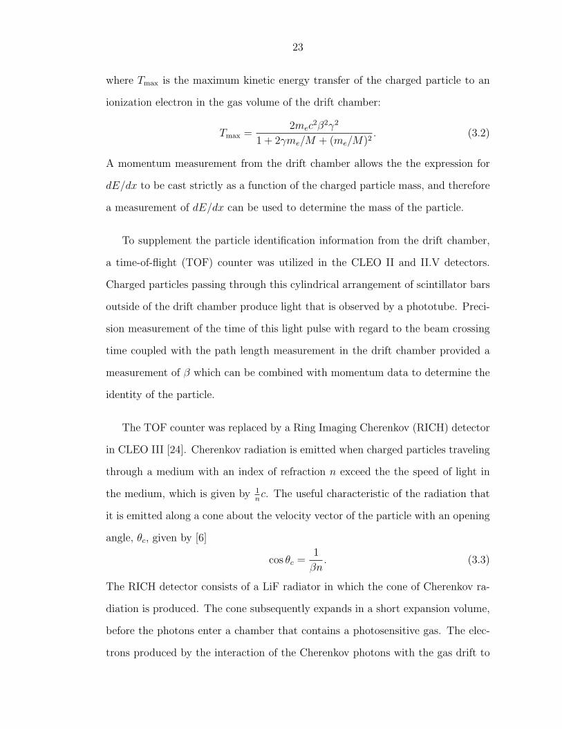
The TOF counter was replaced by a Ring Imaging Cherenkov (RICH) detector

in CLEO III [24]. Cherenkov radiation is emitted when charged particles traveling

through a medium with an index of refraction n exceed the the speed of light in

the medium, which is given by 1nc. The useful characteristic of the radiation that

it is emitted along a cone about the velocity vector of the particle with an opening

angle, θc, given by [6]

cos θc =1

βn. (3.3)

The RICH detector consists of a LiF radiator in which the cone of Cherenkov ra-

diation is produced. The cone subsequently expands in a short expansion volume,

before the photons enter a chamber that contains a photosensitive gas. The elec-

trons produced by the interaction of the Cherenkov photons with the gas drift to

24

anode wires and produce, just as in a drift chamber, an avalanche. Unlike the drift

chamber however, the anode wires themselves are not read out. In the RICH detec-

tor pixelated cathode pads near the anodes are read out to give a two-dimensional

image of the pattern of avalanches. From this image and careful knowledge of the

geometry and track trajectory the Cherenkov cone opening angle and therefore

particle velocity, β, can be determined.

3.2.3 Calorimetry

Photons and other neutral particles will escape the previously mentioned detec-

tors because they are incapable of depositing energy through ionization. Photons

are absorbed by a calorimeter of Thallium-doped Cesium-Iodide (CsI) scintillat-

ing crystals located out outside of the tracking volume and the supplementary

particle identification detectors [25]. Photons entering a crystal produce a shower

of electrons and photons through the repeating processes of pair-production and

bremsstrahlung radiation. Due to the scintillating properties of the crystal, the

intermediate electrons produce light that is registered by a photo-diode that is

optically coupled to the crystal. The entire electromagnetic shower is contained

within a small array of neighboring crystals that can be clustered together in order

to find the precise location and energy of the incident photon.

Similar to photons, electrons shower electromagnetically in the calorimeter. We

use this feature in conjunction with the presence of a drift chamber track pointing

at the shower to identify electrons. Since the energy loss due to bremsstrahlung ra-

diation is proportional to 1/m2, heavy muons pass through the calorimeter without

showering and therefore only leave behind trace amounts of energy.

25

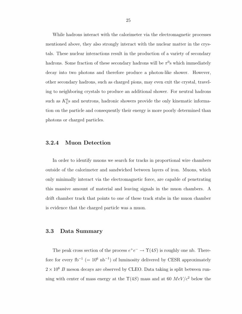
While hadrons interact with the calorimeter via the electromagnetic processes

mentioned above, they also strongly interact with the nuclear matter in the crys-

tals. These nuclear interactions result in the production of a variety of secondary

hadrons. Some fraction of these secondary hadrons will be π0s which immediately

decay into two photons and therefore produce a photon-like shower. However,

other secondary hadrons, such as charged pions, may even exit the crystal, travel-

ing to neighboring crystals to produce an additional shower. For neutral hadrons

such as K0Ls and neutrons, hadronic showers provide the only kinematic informa-

tion on the particle and consequently their energy is more poorly determined than

photons or charged particles.

3.2.4 Muon Detection

In order to identify muons we search for tracks in proportional wire chambers

outside of the calorimeter and sandwiched between layers of iron. Muons, which

only minimally interact via the electromagnetic force, are capable of penetrating

this massive amount of material and leaving signals in the muon chambers. A

drift chamber track that points to one of these track stubs in the muon chamber

is evidence that the charged particle was a muon.

3.3 Data Summary

The peak cross section of the process e+e− → Υ(4S) is roughly one nb. There-

fore for every fb−1 (= 106 nb−1) of luminosity delivered by CESR approximately

2× 106 B meson decays are observed by CLEO. Data taking is split between run-

ning with center of mass energy at the Υ(4S) mass and at 60 MeV/c2 below the

26

Table 3.1: A summary of the three data sets used in this analysis. Due to variationsin the beam energy the ratio of on-resonance luminosity to number of BB eventsis not constant.

Detector Configuration Lon [fb−1] Loff [fb−1] NBB [×106]CLEO II 3.1 1.6 3.3

CLEO II.V 6.0 2.9 6.4CLEO III 6.3 2.3 5.7Total 15.5 6.9 15.4

Υ(4S), below BB threshold. The smaller, latter data set is used to understand

the continuum processes that occur in addition to Υ(4S) production. Table 3.1

summarizes the integrated luminosity (L) and number of Υ(4S) → BB events

used in this analysis. Figure 3.4 shows the data collected per month throughout

the life of the CLEO II, II.V, and III detectors. One notices an increasing trend

in integrated luminosity as a function of accelerator development.

27

1 IR

Bunch Train

CrossingAngle

9 X 2Bunches

Phase IIIR

1st SRF Cavity Installed

9 X 3Bunches

1200

1100

900

800

700

600

500

200

300

100

400

0

1000

1989 1990 19921991 1993 1994 1995 1996 1997 1998

CES

R L

umin

osity

(pb-1

/ Mon

th) 1400

1300

1600

1500

1700

20001999

9 X 4Bunches

2nd SRF Cavity Installed

CLEO IIIInstallation

2001

1800

1900

2000

Figure 3.4: Data collected per month with the CLEO II (pre-1995), II.V (1995-1999), and III (post-1999) detectors. The plot highlights the how the integratedluminosity grows with accelerator developments.

Chapter 4

Experimental Technique

This chapter discusses the reconstruction and selection of the B → Xu`ν can-

didates given the raw information from the detector. The idea is simple: create

an algorithm that preserves as many true B → Xu`ν decays as possible while

rejecting fake candidates. The challenge arises in creating an implementing such

an algorithm.

The only experimentally viable route to obtaining a value of |Vub| is through

the semileptonic charmless decays of B mesons which are complicated by the unde-

tectable neutrino in the final state. A key component of this analysis is therefore

an algorithm which allows the neutrino to be “reconstructed” from the missing

four-momentum in the event. Specifically

pmiss = pinitial −∑

pvisible, (4.1)

where

pinitial = (2Ebeam;−2 sin θcEbeam, 0, 0) (4.2)

is the initial four-momentum of the the two beams1. Ideally pmiss is strictly the

four-momentum of the neutrino in the signal decay. In reality, however, pmiss may

include multiple neutrinos, K0L’s, or neutrons that go undetected along with other

charged tracks and photons that either miss our detector or we have reconstructed

improperly. To eliminate these events with flawed neutrino reconstruction, we

must maximize the resolution of the reconstructed visible four-momentum in the

event which, in turn, maximizes the neutrino resolution. As the neutrino resolution

1θc is the small (≈ 2 mrad) crossing angle of the beams

28

29

increases the kinematic requirements we place on the reconstructed Xu`ν become

more effective at separating the signal events from the background events.

Candidate Reconstruction

In the following sections I will walk through the stages of candidate recon-

struction with an eye towards optimizing the resolution on the four-momentum of

visible particles produced in the e+e− collision. Initially we work to refine the raw

information produced by the detector. From this refined set of visible objects we

can then reconstruct the lepton, hadron, and ultimately neutrino daughters of the

B decay.

4.1 The Fundamental Objects: Tracks and Showers

We can reduce every reconstructed particle in the detector down to a combina-

tion of two fundamental objects: tracks and showers. Ideally, we would like that

each “track” corresponds to the trajectory of a single charged particle produced in

an e+e− collision. We would like, similarly, a “shower” to correspond to the energy

deposited in the calorimeter by a single neutral particle. The spatial location of

the shower and the assumption that it came from the interaction region, we can

deduce the trajectory of the neutral particle that produced it. In reality, such an

ideal list of tracks and showers is not simple to produce.

30

4.1.1 Tracks

To enumerate the particles produced in the collision our goal is this: count

once and only once every charged particle coming from the interaction point. We

rely on the large acceptance of our tracking chamber to try to count every particle.

Unfortunately there are many ways to double count particles, listed below are the

leading contributors:

• Since the chamber is inside of a magnetic field, charged particles with low

transverse momentum will curl inside of the detector. The pattern recogni-

tion software used to find tracks will frequently find multiple tracks from one

curling track as showin in Figure 4.1. This is problematic since it leads to

multiple counting of the same physical particle.

• Some particles, such as charged kaons, decay in flight. The decay produces a

secondary charged particle with a different momentum than the parent and

therefore the track appears to have a kink in it. The pattern recognition will

identify both parts of the track as separate tracks.

• Occasionally, in the case of decays-in-flight or hard scattering where the kink

is small, two tracks will be found. One contains the innermost and outermost

hits while the other contains the hits around the kink. This “ghosting” effect

produces two tracks with similar trajectories for the same physical particle.

Significant work has gone into the development of an algorithms packaged as

Trkman, to recognize and remove these spurious tracks [26]. Tracks that are not

flagged as curlers, ghosts, or decays-in-flight are said to be TrkmanApproved. From

now on “tracks,” unless explicitly stated, refer to TrkmanApproved tracks.

31

3600398-008

Figure 4.1: The pattern recognition code can find multiple tracks for a singlecurling particle.

4.1.2 Showers

Recall that the goal of the calorimeter is to measure every photon leaving the

interaction region. As with tracks, there are methods of producing extra showers in

the calorimeter that are not associated with photons coming from the interaction

of the beams.

• All charged particles will deposit some energy in the calorimeter through

ionization, hadronic interactions, or electromagnetic showers.

• Hadronic interactions within the calorimeter itself or the material just in

front of the calorimeter can create particles that produce an additional sepa-

rate secondary shower away from the primary shower. We call such showers

Splitoff showers.

Showers produced by the first mechanism are eliminated by geometrically match-

ing observed tracks and showers. Recall that in the case of decays-in-flight or

32

hadronic interactions in the tracking volume, one actually wants to match the sec-

ondary tracks, the ones produced by the decay or interaction, to showers in the

calorimeter.

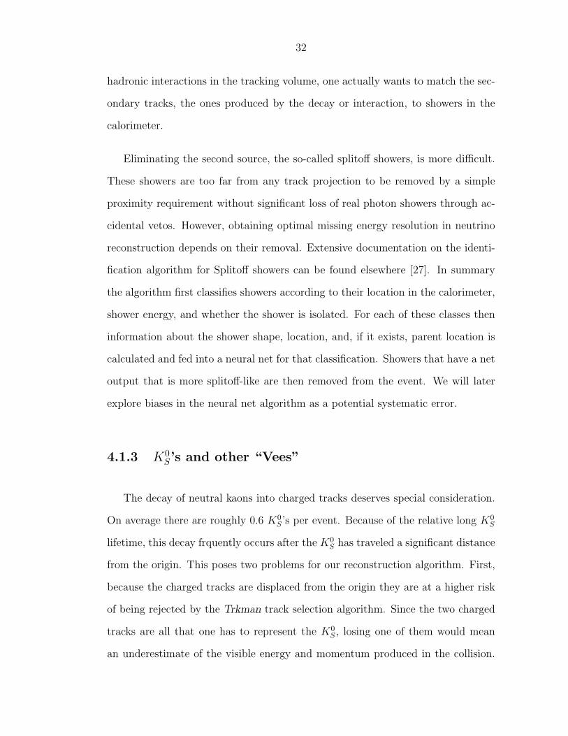
Eliminating the second source, the so-called splitoff showers, is more difficult.

These showers are too far from any track projection to be removed by a simple

proximity requirement without significant loss of real photon showers through ac-

cidental vetos. However, obtaining optimal missing energy resolution in neutrino

reconstruction depends on their removal. Extensive documentation on the identi-

fication algorithm for Splitoff showers can be found elsewhere [27]. In summary

the algorithm first classifies showers according to their location in the calorimeter,

shower energy, and whether the shower is isolated. For each of these classes then

information about the shower shape, location, and, if it exists, parent location is

calculated and fed into a neural net for that classification. Showers that have a net

output that is more splitoff-like are then removed from the event. We will later

explore biases in the neural net algorithm as a potential systematic error.

4.1.3 K0S’s and other “Vees”

The decay of neutral kaons into charged tracks deserves special consideration.

On average there are roughly 0.6 K0S’s per event. Because of the relative long K0

S

lifetime, this decay frquently occurs after the K0S has traveled a significant distance

from the origin. This poses two problems for our reconstruction algorithm. First,

because the charged tracks are displaced from the origin they are at a higher risk

of being rejected by the Trkman track selection algorithm. Since the two charged

tracks are all that one has to represent the K0S, losing one of them would mean

an underestimate of the visible energy and momentum produced in the collision.

33

Secondly, even if the tracks survive the selection cuts the momentum used for each

track is that of the track extrapolated back to the interaction point which is not a

correct representation of the momentum of the particle.

To solve both of these problems we identify K0S’s before filtering out the Trk-

manApproved tracks. We then the kinematically refitted K0S momentum and en-

ergy directly and eliminate the daughter tracks and any curler or ghost track

associated with them.

To select K0S’s we first locate oppositely charged tracks that appear to intersect

at a point displaced from the origin. These tracks are then fit to a common origin

in 3D space [28]. The χ2 of such a fit describes the likelihood that the two tracks

originated from the from the same point, ~d, where ~d is measured from the beam

spot. The fit also produces an error matrix, V , for ~d. In addition the beam spot

has some physical size that is approximately Gaussian in 3D and represented by

an error matrix B. With the “flight significance,” FS, as

FS =

√~d · (V + B)−1 · ~d. (4.3)

we required FS > 7.5 to positively identify a K0S. It is worthwhile to note that

those K0S’s that travel farthest will be easiest to identify. Fortunately, those same

K0S’s are the most problematic for our neutrino reconstruction algorithm. For each

selected K0S, we repeat the kinematic fit with the additional constraint that the

momentum to point back at the beam spot, and all candidates that do not have

a χ2 for three degrees of freedom less than ten are dropped. The resulting π+π−

invariant mass spectrum, fitted to a double Gaussian plus a linear background,

is shown in Figure 4.1.3. We keep candidates within 3σ of the K0S mass, where

σ is the width of the narrower, core Gaussian. These candidates are fit one last

time with the invariant mass of the π+π− constrained to that of the nominal K0S

34

hEntries 63145Mean 0.4988RMS 0.01024

/ ndf 2χ 176.6 / 112 1A 678.4± 1.733e+04 1µ 7.558e-05± 0.4988 1σ 0.0001624± 0.005685

b 36.55± 560.8 m 72.31± -787.1

2A 750.8± 2.557e+04 2µ 2.185e-05± 0.4989 2σ 3.755e-05± 0.002187

]2

Invariant Mass [GeV/c-π+π0.47 0.48 0.49 0.5 0.51 0.52 0.53

2E

ven

ts/0

.5 M

eV/c

0

500

1000

1500

2000

2500

3000

hEntries 63145Mean 0.4988RMS 0.01024

/ ndf 2χ 176.6 / 112 1A 678.4± 1.733e+04 1µ 7.558e-05± 0.4988 1σ 0.0001624± 0.005685

b 36.55± 560.8 m 72.31± -787.1

2A 750.8± 2.557e+04 2µ 2.185e-05± 0.4989 2σ 3.755e-05± 0.002187

data11 (All Selection Cuts)

Figure 4.2: Typical π+π− invariant mass distribution for K0S candidates.

mass. The resulting four-momentum then replaces the daughters, along with all

associated tracks and showers, in the subsequent reconstruction of the event.

One might ask whether such a sophisticated procedure should also be used for

the decay Λ → πp. The average number of Λ’s per event is roughly thirty times less

than the average number of K0S’s so there is little to gain by fitting Λ’s in a similar

fashion. It should be noted that after all of the careful work the effect of “proper”

K0S reconstruction makes a nearly imperceptible difference in the reconstructed

ν resolution. A more significant gain of K0S reconstruction is the elimination of

tracks from the event which in turn reduces combinatoric backgrounds in candidate

reconstruction.

In summary, recall that initial goal of our procedure was a measurement of

the momentum of every particle coming from the collision without any double

counting. To accomplish this, we first identify K0S’s in the event, removing all

tracks and showers associated with the daughters of the K0S’s. Next, we attempt to

filter out the double counted tracks: ghosts, curlers, and decays-in-flight. Finally

35

we remove showers that are associated with particles already measured in the

tracking system.

4.2 Particle Identification

We assume that remaining isolated showers are photons. Tracks, on the other

hand, can be produced b a number of types of charged particles. Particle identifi-

cation is necessary to select the semileptonic decay products calculate the observed

four-momentum in the event that is used in neutrino reconstruction. This section

summarizes how we distinguish among the many species of charged particles for

each track.

4.2.1 Lepton Identification

One of the key signatures of the semileptonic b → u decay is the presence

of a relatively high momentum lepton in the final state; therefore, we take care

to identify leptons with high efficiency. Furthermore, additional leptons in the

event usually indicate more than one neutrino was present in the event. This is

problematic for neutrino reconstruction and we veto events with additional so-

called “counting,” as opposed to “signal,” leptons. A high lepton fake rate will

cause more events to be unnecessarily vetoed.

Electron Identificaiton

Electron identification has long been a recognized sport at CLEO. We use the

accepted Rochester Electron ID algorithm. This algorithm was first developed for

36

CLEO II [29] and was recently revised and improved for use with CLEO II and

CLEO III [30]. Here I review the core ideas of the algorithm and discuss how it is

applied for this analysis.

The primary identifying mark of an electron is that it showers electromagneti-

cally in the calorimeter. Therefore electrons tend to deposit all of their energy in

the calorimeter in a photon-like shower. The hadronic interactions of pions, kaons,

and protons with the calorimeter are much different because the characteristic

nuclear interaction length of a hadronic shower is larger than that of an electro-

magnetic shower. Showers produced by hadronic interactions are distributed across

a larger number of crystals with larger fluctuations in the energy deposition profile

across the crystals. We can pick a set of variables then to discriminate between

electrons and hadrons:

• E/p: The ratio of the energy of the shower to the momentum of the track

as measured in the drift chamber. For reasons discussed above this is near

unity for electrons and typically smaller for hadrons.

• χdE/dxe : Based on specific ionization data from the tracking chamber, this

is the number of standard deviations that the dE/dx measurement for a

particular track deviates from the nominal dE/dx of an electron with that

track’s momentum. The χdE/dxe will generally be near zero for electrons and

away from zero for hadrons.

• w: The RMS width of the shower – narrower for electrons than hadrons.

• ∆θ,∆φ: The deviation of the depth-corrected shower center from the extrap-

olated track trajectory in the θ and φ directions. The large fluctuations in the

energy profile of hadronic showers produce fluctuations in the reconstructed

37

locations of the shower and therefore ∆θ and ∆φ will be distributed more

broadly about zero for hadrons than for electrons.

A pure sample of electrons and positrons can be obtained using radiative Bhabha

events in order to compute the distributions in data for these key variables. Like-

wise, we can use the decay D∗ → Dπ±s , D → K∓π±, where the charge of the

intermediate “slow” pion (πs) tags the identity of the two daughter hadrons, to

obtain pure samples of pions and kaons. These true distributions are then normal-

ized to unit area to form probability distribution functions (pdf’s). The pdf’s are

calculated in bins of track momentum in order to accommodate changes in shower

shape as a function of momentum. A set of typical pdf’s is shown in Figure 4.3

For a given track, we can combine the pdf’s with the measured momentum (p)

and key variable values (xi) to obtain the ratio L of the probabilities that the track

is an electron or a hadron. More formally, L the likelihood ratio, is given by

L =P(x, p)e

P(x, p)h

, (4.4)

where P(x, p)s is the probability that the track is an electron (s = e) or hadron

(s = h). In turn,

P(x, p)s =∏

i

f si (xi; p), (4.5)

where f si (xi; p), is the pdf for a particle of type s in the ith key variable. In practice

we compute ln L which turns the products into sums. Because this ratio is large for

tracks that are electron like, we place a minimum requirement on ln L to identify

electrons. We weigh the electron identification efficiency with the probability that

a pion will fake an electron in determining the minimum acceptable value of ln L.

Specifically we find the minimum ln L such that the probability that a true pion will

be misidentified as an electron is 0.2% (1.0%) in the barrel calorimeter (elsewhere).

38

E/p

dn

/N 1

/dx

e/π Barrel: 0.8 ≤p< 1 GeV/c

0

2

4

6

8

10

12

14

16

0 0.2 0.4 0.6 0.8 1 1.2 1.4

10-1

1

10

10 2

0 0.02 0.04 0.06 0.08 0.1 0.12 0.14 0.16 0.18 0.2|∆Θ|

dn

/N 1

/dx


10-1

1

10

10 2

0 0.02 0.04 0.06 0.08 0.1 0.12 0.14 0.16 0.18 0.2|∆Φ|

dn

/N 1

/dx


Width ALL (cm)

dn

/N 1

/dx


0

0.1

0.2

0.3

0.4

0.5

0.6

0.7

0 1 2 3 4 5 6 7 8 9 10

Figure 4.3: Typical pdf’s for electron identification variables [30]: electron pdfshapes are shown by the open histogram, hadron shapes are shown hatched his-togram.

39

Additionally we use time of flight (RICH) information in CLEO II (III) to veto

tracks that may pass this minimum likelihood cut but otherwise look like hadrons.

In CLEO II we can compute difference in χ2 for the electron and kaon hypotheses

as

∆χ2e/K = χ2TOF

e − χ2TOF

K . (4.6)

For true electrons this quantity tend negative, while for true kaons the χ2TOF

K will be

at a minimum and the difference will tend to be positive. We require ∆χ2e/K < 10

to veto kaons that may fake electrons.

Using the RICH detector in CLEO III we can compute the likelihood that a

particular track is an electron, pion, proton, or kaon. This allows us to reduce

the probability that hadrons will fake electrons, especially in momentum regions

where the dE/dx seems ambiguous. If the likelihood that particle of momentum

p is of species, s, as determined by RICH information is Ls then we require:

Le > Lπ if p < 500 MeV/c, (4.7)

Le > LK if 500 MeV/c < p < 800 MeV/c, and (4.8)

Le > Lp if 900 MeV/c < p < 1.7 GeV/c. (4.9)

Tracks with momenta greater than 200 MeV/c that pass all of the criteria listed

above are declared “electrons.” The identification efficiency as a function of mo-

mentum is shown in Figure 4.4. From this set of electrons we select the “signal

electrons” that will be used in reconstructing the exclusive B → Xueν decays. To

qualify as a signal electron the electron must also:

• have a momentum greater than 1.0 GeV/c

• have hits in at least 40% of the drift chamber layers the that track passed

through

40

[GeV/c]ep0.5 1 1.5 2 2.5 3

Eff

icie

ncy

0

0.1

0.2

0.3

0.4

0.5

0.6

0.7

0.8

0.9

1

Rochester Electron ID

Figure 4.4: Electron identification efficiency as a function of momentum using theRochester Electron ID algorithm. Data shown are for CLEO III – efficiencies inCLEO II and II.V are similar.

• have a distance of closest approach to the beam spot less than 2 mm in the

plane transverse to the beam axis

• have a distance of closest approach to the beam spot less than 5 cm is the z

direction.

These criteria yield a relatively pure sample of signal electrons with efficiency

typically greater than 95% for electrons resulting from semileptonic b→ u decay.

Identifying Muons

Much like electrons, muons have characteristic qualities that make them easy

to identify. They are heavy particles that interact only via the electromagnetic and

weak forces. At momenta relevant for CLEO, the primary mechanism of energy

loss for muons traveling through material is ionization. As a result, muons can

41

penetrate through much more material than electrons or hadrons, whose ranges are

limited by the much strong electromagnetic and additional hadronic interaction,

respectively. We denote the depth that the muon penetrates by the number of

hadronic interaction lengths, Xµ. Our muon chamber allows coverage over region

|cos θ| < 0.85 (0.65) for CLEO II (III).2 If a track within this fiducial volume that

has not been identified as an electron satisfies

• p > 1.2 GeV/c and Xµ ≥ 5 or

• 1.0 GeV/c ≤ p < 1.75 GeV/c and 3 ≤ Xµ < 5,

we classify it as a “counting muon.” Of these muons, we select a subset of “signal

muons” for reconstructing the B → Xuµν decays that:

• have Xµ ≥ 5,

• have hits in at least 40% of the drift chamber layers the that track passed

through,

• have a distance of closest approach to the beam spot less than 2 mm in the

plane transverse to the beam axis,

• and have a distance of closest approach to the beam spot less than 5 cm is

the z direction.

The efficiencies for these “counting” and more-restrictive “signal” muons are shown

in Figure 4.5. Because softer muons will lose all of their momentum through specific

ionization before penetrating deeply into the detector, the Xµ ≥ 5 requirement

greatly reduces the identification efficiency for signal muons below 1.5 GeV/c.

2The reduced muon identification volume in CLEO III is due to excessive beam relatednoise in the endcap muon chambers that posed a problem with reconstruction.

42

[GeV/c]µp1 1.2 1.4 1.6 1.8 2 2.2 2.4 2.6

Eff

icie

ncy

0

0.1

0.2

0.3

0.4

0.5

0.6

0.7

0.8

0.9

1

Signal Muons

[GeV/c]µp1 1.2 1.4 1.6 1.8 2 2.2 2.4 2.6

Eff

icie

ncy

0

0.1

0.2

0.3

0.4

0.5

0.6

0.7

0.8

0.9

1

Counting Muons

Figure 4.5: Muon identification efficiency as a function of momentum for signalmuons (left) and counting muons (right). Data shown are for CLEO III – efficien-cies in CLEO II and II.V are similar.

4.2.2 Hadron Identification

Once the electrons and muons have been identified, we then classify the remain-

ing tracks in the event as pions, kaons, or protons using two pieces of information.

First we use the probability that a particle is a particular species, which we obtain

by combining the dE/dx in the drift chamber with the time of flight or RICH

information. Let’s call this the “detector” probability PsD that the particle is of

type s. The second piece of information is the relative multiplicites of pion, kaons,

and protons in generic B decay. That is, given a sample of charged particles at

a particular momentum from a large number of B decays, what fraction will be

pions, what fraction kaons, and what fraction protons? We will weight the proba-

bilities based on the detector information by these production fractions, which we

denote as PsP . How do we determine Ps

D and PsP ?

For a set of true pions, kaons, or protons of a given momentum the time of

flight and dE/dx will be Gaussian distributed variables. The raw dE/dx and time

43

of flight information in CLEO II can therefore be used to calculate an absolute

probability that a particle is a particular species. If either the dE/dx or time of

flight information is missing, for example, if the particle curls in the magnetic field

and does not reach the time of flight counters, then we calculate PsD solely from

the available measurement.

In CLEO III we use the dE/dx information along with information from the

RICH detector. Unfortunately the calculation of pure detector probabilities for

particular particle species is not as straightforward in CLEO III. For example in

CLEO II we could determine the absolute probability that a particle was pion or

a kaon, but in CLEO III we must ask whether a particle is more pion-like than

kaon-like.

We can, however, mock up a number that behaves like PsD. As an example I

will discuss how we generate PπD and PK

D . The dE/dx reconstruction code provides

χdE/dxπ . The RICH system provides us the quantity χ2RICH

π = −2 ln Lπ, which

is related to the likelihood that the track is a pion. However, χ2RICH

π only has

meaning when compared with another likelihood, χ2RICH

K , it has no meaning in an

absolute sense. We can still assign relative pion and kaon probabilities using the

construction

χ2 = χ2dE/dx

K − χ2dE/dx

π + χ2RICH

K − χ2RICH

π . (4.10)

When χ2 is zero the track looks just as much like a pion as a kaon. For positive or

negative numbers the track is more pion- or kaon-like respectively. We now map

χ2 onto a function that looks like a probability by defining

PπD =

1− 1

2e−χ2

if χ2 ≥ 0

12eχ2

if χ2 < 0,

(4.11)

PKD = 1− Pπ

D. (4.12)

44

In a similar fashion we define PpD with respect to PK

D . Using this technique for

CLEO III we are able to generate the probabilities, PsD, that can be used in the

same way as the calculated CLEO II probabilities.

From our Monte Carlo model of generic B decays we obtain a parameterization

of the production fractions PsP as a function of particle momentum p given by

PKP (p) =

0.277p− 0.107p2 if p < 2.0 GeV/c

0.06 if p ≥ 2.0 GeV/c,

(4.13)

PpP (p) = 0.02, (4.14)

PπP (p) = 1− PK

P (p)− PpP (p). (4.15)

We calculate a relative “probability” that the track is of species s, Ps by mul-

tiplying PsD · Ps

P (p). We then assign a particle an identification, s, based on which

hypothesis, π, K, or p, gives the maximum Ps. Note that pions are the dominant

particle produced in B decay. Assuming detector information is inconclusive for a

particular track we would still like to enforce what know about B decays to call

that track a pion.

4.2.3 Monte Carlo Considerations

We need our analysis code to produce the same results, that is, efficiencies and

fake rates, when run over Monte Carlo as when run over data. Perfect agreement

is challenging in the area of lepton identification. Electron identification depends

strongly on the shapes of calorimeter showers which can be difficult to model in

Monte Carlo. The simulation also overestimates the rate for pions to fake muons.

To remedy these problems we employ a special technique when identifying letpons

in Monte Carlo.

45

In order to identify Monte Carlo electrons we consider only tracks that satisfy

the quality requirements above and that are tagged to generated electrons. We

measure the identification efficiency as a function of momentum in data using ra-

diative Bhabha events embedded into hadronic events [30]. We throw a random

number between zero and one and if the thrown number is less than the efficiency

we identify the track as an electron. This ensures that we have the same identifi-

cation efficiency on average in Monte Carlo that we do in data.

For muons we also only consider tracks which are tagged to generated muons. In

CLEO II we have verified that the Monte Carlo correctly predicts the identification

efficiency for true MC muons. With regard to CLEO III we apply an event weight

that corrects the Monte Carlo identification efficiency for problems in simulating

early features of the muon hardware readout . We will postpone a discussion of

“event weights” in general until Section 5.2. Complete details of the CLEO III

muon efficiency study can be found in Appendix A.

The procedure just outlined in the previous paragraph allows us reproduce the

correct identification efficiency for true leptons. However, this procedure does not

yield a background estimate for hadrons faking leptons. As will be discussed later,

we require exactly one lepton in the event, and some fraction of the “extra leptons”

arise from hadrons faking leptons. We therefore need measurements of the rates

for hadrons to fake leptons both to estimate the fake signal lepton background

contributions (see Section 5.3.3) and to simulate the efficiency loss when these

fakes result in an extra lepton in the event.

We measure the probability for hadrons to fake leptons as a function of momen-

tum in data, using clean samples of pions, kaons, and protons3. The probability

3Appendix A discusses this measurement for muons in CLEO III

46

that there will be no fake leptons in the event can be written as

P!fake =∏

hadrons

(1− Ps

µ fake(p))(1− Ps

e fake(p)) , (4.16)

where Psµ fake(p) or Ps

e fake(p) is the probability for a track of species s and momen-

tum p to fake a muon or electron. A random number between zero and one will

then be greater than P!fake with a probability equal to that of having one or more

fake leptons in the event. Events for which this is the case can therefore be vetoed

in Monte Carlo at the same rate that they are in data.

It is only lepton identification efficiencies and fake rates in Monte Carlo that

require sophisticated tuning to be certain that analyzing Monte Carlo and real

data produce the same results. Studies have verified that the Monte Carlo does a

sufficiently good job and modeling dE/dx, RICH, and time of flight information

used in hadron identification within reasonable systematic uncertainties which we

will explore in Chapter 6.

4.3 Signal Hadron Reconstruction

In our quest to reconstruct B → Xu`ν decays we devote this section to iden-

tifying and reconstructing the Xu part of the decay. Given the work described

above, the task of assembling unique pions and photons into signal hadrons is

quite simple.

We would like to reconstruct Xu candidates of the following types: π±, π0, η,

ρ±, ρ0, and ω. Table 4.1 summarizes the decay modes that we reconstruct for each

of these hadrons. Note that all of the final states are a combination of charged

pions and photons. We require that the pions be identified as pions by the particle

47

Table 4.1: A summary of the reconstructed hadron final states.

Xu Final Stateπ± π±

π0 γγη γγ; π+π−π0, π0 → γγρ± π±π0, π0 → γγρ0 π+π−

ω π+π−π0, π0 → γγ

identification algorithm discussed above and that they not be the daughter of a

reconstructed K0S.

In all instances where we reconstruct the the decay of η or π0 to γγ we perform

a kinematic fit that constrains the invariant mass of the photons to the nominal

mass of the η or π0. We require that this fitting procedure not “pull” the invariant

mass more than two standard deviations from its raw value. This produces a

resolution dependent cut on the invariant mass of the reconstructed photons. On

average, this cut eliminates candidates more than 8 MeV/c2 (26 MeV/c2) from

the nominal π0 (η) mass.

In all other cases, kinematic fits are not performed. We accept η (ω) candidates

decaying into π+π−π0 that are within 10 (30) MeV/c2 of the nominal η (ω) mass.

In order to have sufficient efficiency when reconstructing the inherently wide ρ, we

accept all ππ candidates within 285 MeV/c2 of nominal ρ mass.

We will revisit the topic of signal hadron reconstruction briefly when we discuss

B → Xu`ν candidate selection later in Section 4.9. There we will mention addi-

tional requirements that can placed on the hadron candidates in order to increase

the probability that we pick a real B → Xu`ν decay over some other combination

of random particles in the event.

48

4.4 Final Candidate Reconstruction

Let’s begin this section by summarizing what we have discussed so far in this

chapter. We have taken tracking and calorimetry information and attempted to

produce a complete set of unique momentum measurements for each particle leav-

ing the interaction region. From the tracks we first select the electrons and muons,

and then we used remaining detector information and our knowledge of production

fractions to classify the remaining hadrons as pions, kaons, or protons. Once the

particle identification step is complete we now have a complete picture, i.e. the

four-momenta, of all of the visible particles produced in the collision.

For our current purposes, let us assume for the moment that pmiss, as defined in

Equation 4.1, is the measured four-momentum of the signal neutrino, pν . As can be

seen in Figure 4.6, the resolution of the reconstructed neutrino is quite poor with

regard to the expected resolution of the any of the visible particles in the event.

We have an opportunity, given what we know about the rest of the B → Xu`ν

candidate, to refine the kinematic properties of this reconstructed neutrino.

Note that the missing energy component of the neutrino four-momentum is

more poorly measured than the missing three-momentum. The two chief reasons

for this are:

• Because momentum is a vector quantity, mistakes distributed uniformly in

all directions tend to cancel out. With the scalar energy, similar mistakes

such as a little extra noise spread out in the calorimeter have an additive

effect.

• The momentum of track is derived directly from the curvature in the drift

chamber. Determining its energy however requires knowing what its iden-

49

[GeV]ν-EmissE-2 -1 0 1 2 3 40

1000

2000

3000

4000

5000

Monte Carloνl±π→B

All Events = 1

leptonQ = 0 and N

[GeV/c]ν-|p|miss|p|-2 -1 0 1 2 3 40

2000

4000

6000

8000

10000

12000

Monte Carloνl±π→B

All Events = 1

leptonQ = 0 and N

Figure 4.6: A plot of the difference between reconstructed and generated missingenergy (left) and missing momentum (right). The resolutions can be improved byrequiring the net charge of all tracks to be zero and the number of leptons in theevent be just one, the signal lepton. Both of these criteria remove events with extraparticles. (The dotted histogram has been scaled to allow an easy comparison.)

tity is. Therefore, the missing energy calculation is susceptible to particle

identification mistakes.

Knowing that neutrinos are effectively massless we can use the magnitude of the of

the missing momentum to set the energy of the neutrino. We refine the neutrino

four-momentum by setting

pν → (|~pν | , ~pν) . (4.17)

Using this modified neutrino four-vector we can now fold in the next piece of

information: the energy of our reconstructed B decay should be equal to the energy

of one of the beam particles. In the process Υ(4S) → BB each B carries away

the same energy as one of the beam particles. We can therefore define the variable

50

∆E as

∆E = Efinal − Ebeam (4.18)

= (EXu + E` + |~pν |)− Ebeam. (4.19)

This variable is of great importance as the true signal candidates will peak at

∆E = 0. Assuming that for a given signal decay the deviation from ∆E = 0

arises predominantly from measurement errors in the magnitude of the missing

momentum, we can scale the neutrino momentum ~pν by a parameter α to force

∆E → 0. We can compute α from the expression above as

α ≡ 1

|~pν |(Ebeam − EXu − E`) . (4.20)

We further refine our neutrino reconstruction by incorporating this energy adjust-

ment and setting

pν → (α |~pν | , α~pν) . (4.21)

One final constraint remains: the mass of the reconstructed B meson should

equal the nominal B mass. Since we know the energy of the B is equal to Ebeam,

a quantity known very well, we can define the reconstructed B mass, Mh`ν as:

Mh`ν =

√E2

beam − | ~pB|2 (4.22)

=

√E2

beam − |~pXu + ~p` + α~pν |2. (4.23)

True signal candidates will peak at Mh`ν = MB.

Finally, we assume that any deviation from the nominal value for a true signal

candidate is due to an error in the reconstruction of the direction of the neutrino

momentum. If we divide ~pB into two components ~pν and ~ph`, where ~ph` ≡ ~pXu +~p`,

we can force Mh`ν → MB by rotating the neutrino momentum, ~pν , in the plane

51

defined by ~ph`× ~pν . Specifically, we rotate the neutrino to enforce the relationship

cos θν−h` =E2

beam −M2B − α2~p2

ν − ~p2h`

2 |α~pν | |~ph`|, (4.24)

where θν−h` is the angle between ~ph` and ~pν . We discard candidates for which

the above expression for cos θν−h` results in an unphysical angle. If we call R the

rotation matrix that forces Mh`ν → MB, we can reset the neutrino momentum,

now incorporating all that we know about the candidate, to

pν → (α |~pν | , αR~pν) . (4.25)

We use this highly refined value of the neutrino four-momentum to maximize

our resolution in the momentum-transfer variable q2:

q2 ≡ |pν + p`|2. (4.26)

At this point I have outlined the algorithm for identifying and reconstruction

B → Xu`ν candidates within an event. In the coming sections I will discuss how

to separate the real B → Xu`ν from the enormous experimental backgrounds that

are present. In the end we seek to represent the data in such a way that the signal

appears as a peak on a smooth background for the purpose of extracting the signal

with a fit. The variables ∆E and Mh`ν defined in this section permit the data to

be represented in such a way.

Candidate Selection

Now that we have the ability to reconstruct B → Xu`ν candidates we are faced

with the daunting task of trying to separate the real signal candidates from the

background. While I postpone a full discussion of fitting and extracting a signal

52

until the next chapter it is impossible to present the ideas of candidate selection

without some general idea of how the data will be fit. When we attempt to fit

the data we will have a collection events from the detector. Some fraction of these

events will be signal and some fraction will be background. The purpose of the

fit is to determine these relative fractions. Most importantly, we are interested in

knowing the number of signal events. The ability of the fit to discriminate between

signal and background depends on two things:

• the difference in shape between the signal and background

• and the statistical significance of the signal compared to the background.

In order to aid the fitter with the first of these we choose to bin the data two-

dimensionally in the variables ∆E and Mh`ν as described in the previous section.

In these variables the signal peaks and the background is relatively smooth allowing

maximum shape discrimination. The second of these points will be the subject of

the rest of this chapter. We must find a collection of analysis requirements which

maximize the number of signal events with respect to background events.

It is important to note all of the selection studies were performed on Monte

Carlo that is independent of the Monte Carlo used in the final fit. Furthermore,

no selection studies were performed using the actual data collected with the detec-

tor. By using a Monte Carlo sample for tuning the analysis requirments that is

independent of the sample used for fits to the data, we avoid biasing our final fit

by accidentally tuning on a statistical fluctuation of the Monte Carlo.

53

4.5 Figures of Merit

To evaluate the impact of any particular selection criteria in the analysis it is

necessary to define a “figure of merit” (F), which in our case is directly related to

the total significance of the extracted rates. The figure of merit becomes the yard-

stick for fine tuning the analysis. Because of its importance helping us achieve the

maximum statistical significance of the result and its central role in later discus-

sions, I undertake a rigorous development in this section. Note: in the discussion

that follows I will use σ for statistical errors, s for systematic errors, and δ for

combined systematic and statistical errors.

4.5.1 A Basic Figure of Merit

As a starting point, let’s consider the figure of merit

F =Ns√

Ns +Nb

, (4.27)

where Ns and Nb are the number of signal and background events in the signal

bin. F is simply the significance of the signal because

σNs =√Ns, (4.28)

σNb=

√Nb, (4.29)

and Ns by the quadrature sum yields the significance.

This simple figure of merit is inadequate for our use because it assumes that one

can subdivide the signal and background contributions to the total yield with infi-

nite precision. In both cases these distributions have finite statistics which should

be considered when evaluating a figure of merit. We can expand the expression for

54

Nb as

Nb = Nb→c +Nb→u +Ncont. (4.30)

The first and most significant component of the background comes from generic

b→ c decays and is modeled by a five-times luminosity set of Monte Carlo. There-

fore the counting error on this distribution will be equal√

5Nb→c, but this counting

error will enter with a factor of 15. In addition we include an estimated 10% sys-

tematic error on Nb→c due to imperfect modeling of the Monte Carlo in the total

uncertainty estimate of Nb→c:

σNb→c=

√Nb→c +

(1

5

)2

5Nb→c, (4.31)

sNb→c= 0.1Nb→c. (4.32)

The background from the non-BB continuum, Ncont, will be derived from data

taken below the Υ(4S) resonance. This data set is only one half of the size of

the on-resonance data, so the distribution must be scaled up instead of down like

the b → c distribution. Because the distribution does come from data there is no

systematic component in the error. We can summarize the error on Ncont as

σNcont =

√Ncont + 22

1

2Ncont. (4.33)

The final background component comes from other b → u decays that feed

into the particular signal we are trying to extract. These decays are modeled with

roughly twenty-times luminosity so we can neglect any counting error on the model

distribution for the purposes of tuning our selection criteria. Simplifying we can

rewrite the error on Nb:

σNb=

√1.2Nb→c + 3Ncont +Nb→u, (4.34)

sNb= 0.1Nb→c. (4.35)

55

Using this more careful estimate of the error on the number of background

events we can revise F to include the finite Monte Carlo statistics used in the

measurement. For a single measured yield we therefore have

F =Ns√

σ2Ns

+ σ2Nb

+ s2Nb→c

. (4.36)

4.5.2 A Figure of Merit for a Rate Measurement

We are interested in producing a single rate measurement for the π−`+ν and

ρ−`+ν modes in each q2 bin and also for the η mode. In order to do this we must

measure the efficiency corrected yield of these decays. We make this measurement

from a combination of several independent rates. For example, in the π−`+ν mode,

we will have the π±`ν and π0`ν samples, each of which will be divided into net

charge ±1 and net charge 0 samples. We average these independent measurements

and enforce isospin symmetry to produce a final π−`+ν measurement.

When averaging π±`ν and π0`ν to determine a combined B → πlν event count

cross feed exists and the two measurements are no longer independent. We will

ignore correlations of this type in the final figure of merit calculation. However,

there are correlated systematic errors, such as the 10% b→ c modeling error, that

cannot be ignored when averaging samples.

Assuming a set of cuts with signal efficiency εi produces a sample with Nsiand

Nbisignal and background events one can calculate the efficiency corrected number

of signal events, denoted Ni, as

Ni =1

εiNsi

, (4.37)

56

with statistical and correlated systematic errors:

σNi=

√(1

εiσNsi

)2

+

(σεi

εi

1

εiNsi

)2

, (4.38)

sNi=

1

εisNb

. (4.39)

The error σεiis the uncertainty on the efficiency of the ith sample. For our tuning

purposes we assume that this error is due strictly to the finite statistics of the Ngen

signal Monte Carlo events used to evaluate the efficiency and does not contain any

systematic component. The error, given by the binomial distribution, is therefore

σεi=

√εi (1− εi)

Ngen

. (4.40)

We can then make a weighted average of event measurements made with the n

(assumed independent) samples. The average number of signal events N is given

by

N =

∑ni=1wiNi∑n

i=1wi

, (4.41)

where we weight the samples by their overall significance using the weights

wi =1

σ2Ni

+ s2Ni

. (4.42)

Careful consideration is necessary when computing the error on the average

given by Equation 4.41 if there are significant correlations in the sample. In the

end we are interested in the significance of the average measurement, so an in-

correct error calculation will easily lead us astray. Given that each independent

measurement, Ni, has an uncorrelated statistical error σNiand a fully correlated

systematic error sNi, we can write the n× n covariance matrix as

Cij =

σ2Ni

+ s2Ni

if i = j,

sNisNj

if i 6= j.

(4.43)

57

Using this covariance matrix we can compute the variance of N , VN ,

VN =n∑

i=1

n∑j=1

∂N∂Ni

Cij∂N∂Nj

(4.44)

=n∑

i=1

n∑j=1

wi

WCij

wj

W(4.45)

=1

W 2

[n∑

i=1

w2i

(σ2Ni

+ s2Ni

)+ 2

n∑i=1

n∑j=i+1

wiwjsNisNj

](4.46)

=1

W+

2

W 2

n∑i=1

n∑j=i+1

wiwjsNisNj

, (4.47)

where W ≡∑n

i=1wi. The first term in the last expression above is the contribution

of the n independent uncorrelated samples, while the second term inflates the error

appropriately to account for the correlations. Given the weighted average signal

measurement and its variance we can trivially define a figure of merit related to

the significance of the measurement as

F =NδN

=N√VN

. (4.48)

This is the figure of merit that we use to tune the selection criteria for the analysis.

4.6 Continuum Suppression

The largest and fortunately easiest to suppress background comes from the

production of qq pairs, where q = u, d, s, or c. Approximately 75% of the cross

section for e+e− → hadrons at the Υ(4S) is of this type. We are able to separate

these events from those events in which a pair of B mesons was produced by

examining the shape of the event. We do this using the technique of a Fisher

Discriminant [31].

58

4.6.1 Event Shape Variables

If we have an event of the type e+e− → qq where q = u, d, s, or c, the sum of

the final state quark masses is much less than the total center of mass energy of

the collision. To conserve four-momentum the quarks leave the interaction region

back-to-back with large velocities. Because of this, they subsequently hadronize

into two collinear jets of hadrons.

In our signal BB events, on the other hand, the particles tend to be distributed

isotropically. In the case of e+e− → Υ(4S) → BB the two B mesons are produced

essentially at rest in the laboratory frame. They each subsequently explode into

hadrons spraying particles uniformly in all directions. Furthermore the kinematics

of a particular B decay is completely uncorrelated from the kinematics of the other

B decay.

It is this shape difference, “jetty” versus isotropic, that allows us to discriminate

between BB events and continuum qq events. In order utilize this shape difference

we must define a suitable set of variables to quantitatively describe the shape of

the events. One such variable is the “thrust axis,” ti, for a set of i particles. We

define the thrust axis as the unit vector that maximizes the thrust, t, where

t ≡∑

i

~pi · ti. (4.49)

It will be useful to consider the thrust axes of our candidate particles, the

particles in the rest of the event, and the entire event. We can define these as

tcand, tROE, and tevent respectively.

To see the usefulness of this quantity, consider a continuum event where all of

the particles are collimated into two jets. As a result,∣∣tcand · tROE

∣∣ will peak near

59

|ROEt candt|0 0.1 0.2 0.3 0.4 0.5 0.6 0.7 0.8 0.9 1

0

1000

2000

3000

4000

5000

6000

7000

8000

Figure 4.7: A comparison of∣∣tcand · tROE

∣∣ for B → π`ν sig-nal Monte Carlo (shaded) and off-resonance continuum data (open).

R20 0.1 0.2 0.3 0.4 0.5 0.6 0.7 0.8 0.9 1

0

1000

2000

3000

4000

5000

6000

Figure 4.8: A comparison of R2for B → π`ν signal Monte Carlo(shaded) and off-resonance contin-uum data (open).

one (shown in Figure 4.7). That is to say, the two thrust axes will be aligned.

We do not include the neutrino momentum in the calculation of tcand to avoid the

inherit correlation between it and the other particles in the event from which it is

derived.

Additionally we use the ratio, R2 ≡ H2/H0, of the second to zeroth Fox-

Wolfram moments [33]. The lth Fox-Wolfram moment for a set of i particles is

defined as

Hl ≡(

4π

2n+ 1

) l∑m=−l

∣∣∣∣∣∑i

Y ml (Ωi)

|~pi|√s

∣∣∣∣∣2

, (4.50)

where s is the total center of mass energy squared, and the Y ml ’s are the familiar

spherical harmonics. The jet structure present in continuum events enhances the

second moment and therefore the ratio R2 tends to one for jetty continuum events

and to zero for isotropic BB events as shown in Figure 4.8.

The two variables defined above,∣∣tcand · tROE

∣∣ and R2, provide very good dis-

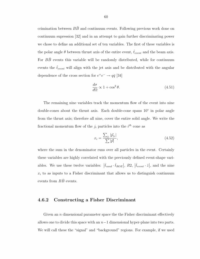
60

crimination between BB and continuum events. Following previous work done on

continuum supression [32] and in an attempt to gain further discriminating power

we chose to define an additional set of ten variables. The first of these variables is

the polar angle θ between thrust axis of the entire event, tevent and the beam axis.

For BB events this variable will be randomly distributed, while for continuum

events the tevent will align with the jet axis and be distributed with the angular

dependence of the cross section for e+e− → qq [34]

dσ

dΩ∝ 1 + cos2 θ. (4.51)

The remaining nine variables track the momentum flow of the event into nine

double-cones about the thrust axis. Each double-cone spans 10 in polar angle

from the thrust axis; therefore all nine, cover the entire solid angle. We write the

fractional momentum flow of the ji particles into the ith cone as

xi =

∑ji|~pji|∑

|~p|, (4.52)

where the sum in the denominator runs over all particles in the event. Certainly

these variables are highly correlated with the previously defined event-shape vari-

ables. We use these twelve variables:∣∣tcand · tROE

∣∣, R2,∣∣tevent · z

∣∣, and the nine

xi to as inputs to a Fisher discriminant that allows us to distinguish continuum

events from BB events.

4.6.2 Constructing a Fisher Discriminant

Given an n dimensional parameter space the the Fisher discriminant effectively

allows one to divide this space with an n−1 dimensional hyper-plane into two parts.

We will call these the “signal” and “background” regions. For example, if we used

61

only two variables for continuum suppression, constructing a Fisher discriminant

would essentially pick the line that best divided the two-dimensional space such

that signal events most frequently fell on one side of the line while background

events most frequently fell on the other side.

Operationally, we find a set of “Fisher weights” that determine the slope of

the hyper-plane in each of the dimensions. These weights are picked by examining

a set of pure simulated signal events and a set of simulated background events.

Defining the twelve-dimensional covariance matrix of our continuum suppression

variables as C and each variable has a mean µi, then the optimal Fisher weights,

αi are given by

αi ≡12∑

j=1

(Csig + Cbkg

)−1

ij×

(µbkg

i − µsigi

). (4.53)

We can then define the Fisher discriminant, DF , for our set of twelve event-

shape variables, λi, as

DF ≡12∑i=1

αiλi. (4.54)

Examining the two equations above gives insight as to how the discriminant

functions: we weight more heavily those variables with means that differ signif-

icantly in the two samples. The order of subtraction in the weight evaluation

(Equation 4.53) pushes the discriminant more positive for background-like events

and more negative for signal-like events. By cutting all events above some maxi-

mum DF we can remove a substantial fraction of the continuum-like events. From

the multidimensional space perspective, the weights determine the orientation of

the hyper-plane and the cut we choose translates the dividing plane in the remain-

ing orthogonal dimension. We use the figure of merit to select the most optimal

cut.

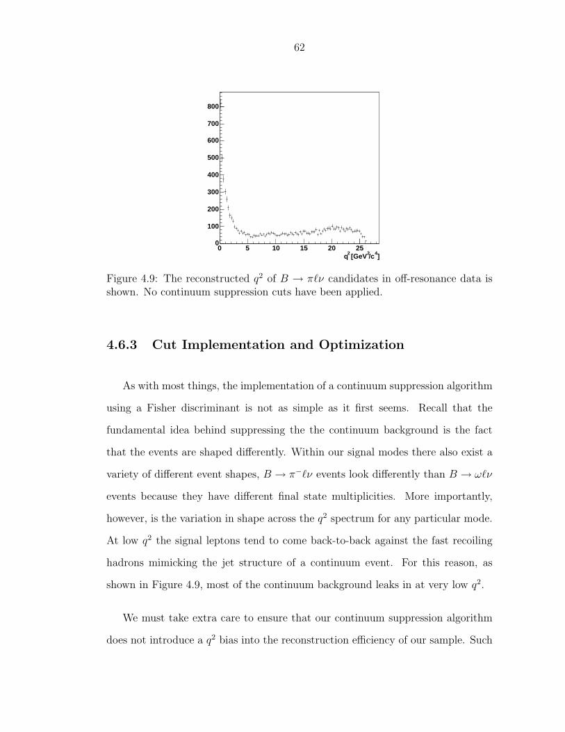
62

]4/c2 [GeV2q0 5 10 15 20 25

0

100

200

300

400

500

600

700

800

Figure 4.9: The reconstructed q2 of B → π`ν candidates in off-resonance data isshown. No continuum suppression cuts have been applied.

4.6.3 Cut Implementation and Optimization

As with most things, the implementation of a continuum suppression algorithm

using a Fisher discriminant is not as simple as it first seems. Recall that the

fundamental idea behind suppressing the the continuum background is the fact

that the events are shaped differently. Within our signal modes there also exist a

variety of different event shapes, B → π−`ν events look differently than B → ω`ν

events because they have different final state multiplicities. More importantly,

however, is the variation in shape across the q2 spectrum for any particular mode.

At low q2 the signal leptons tend to come back-to-back against the fast recoiling

hadrons mimicking the jet structure of a continuum event. For this reason, as

shown in Figure 4.9, most of the continuum background leaks in at very low q2.

We must take extra care to ensure that our continuum suppression algorithm

does not introduce a q2 bias into the reconstruction efficiency of our sample. Such

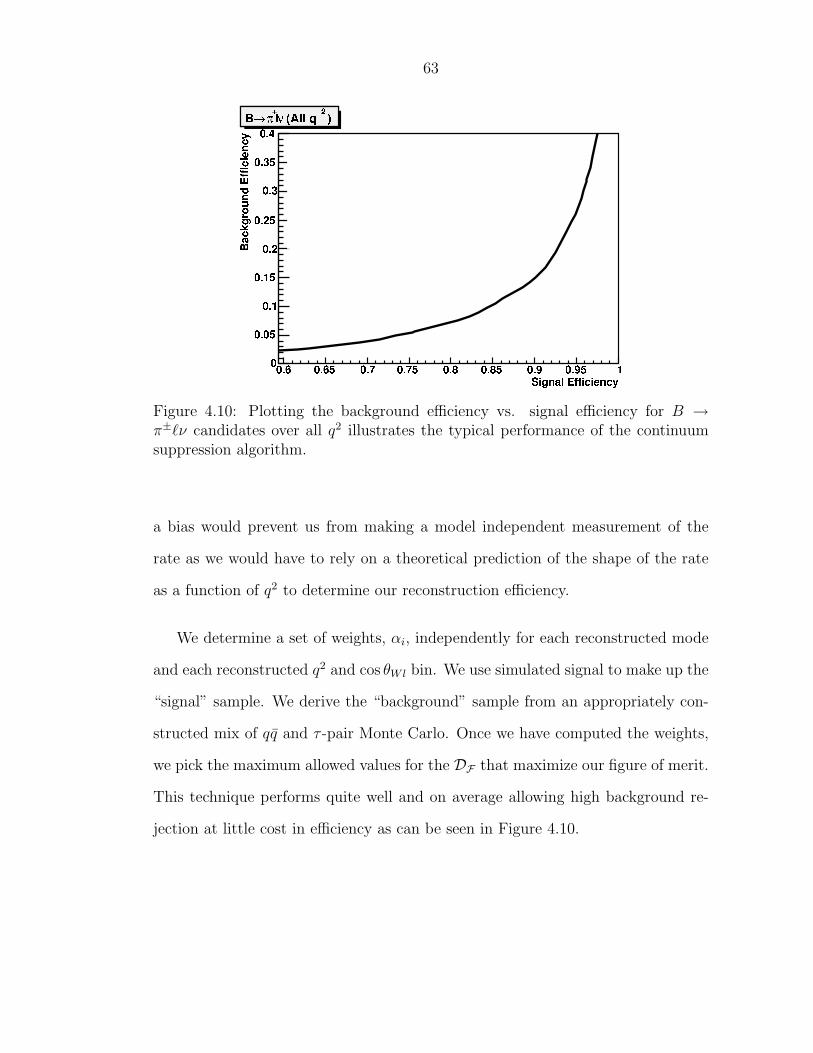
63

Figure 4.10: Plotting the background efficiency vs. signal efficiency for B →π±`ν candidates over all q2 illustrates the typical performance of the continuumsuppression algorithm.

a bias would prevent us from making a model independent measurement of the

rate as we would have to rely on a theoretical prediction of the shape of the rate

as a function of q2 to determine our reconstruction efficiency.

We determine a set of weights, αi, independently for each reconstructed mode

and each reconstructed q2 and cos θWl bin. We use simulated signal to make up the

“signal” sample. We derive the “background” sample from an appropriately con-

structed mix of qq and τ -pair Monte Carlo. Once we have computed the weights,

we pick the maximum allowed values for the DF that maximize our figure of merit.

This technique performs quite well and on average allowing high background re-

jection at little cost in efficiency as can be seen in Figure 4.10.

64

4.7 b→ c Background

After eliminating the large continuum background, we are left with the favored

b→ c decay of the B meson as our dominant background. As will be shown, some

of this background can be reduced with lepton momentum and track multiplicity

requirements. However, this background can not be eliminated as effectively as

the continuum background. It remains as the dominant background that we must

model and account for in the fit.

4.7.1 Lepton Momentum Requirement

Leptons arise from “charmed” B decay in one of two ways: “primary” leptons

from b→ c`ν transitions and “secondary” leptons from b→ c→ s`ν decays. The

characteristic spectra of these decays along with our signal b → u`ν decays are

shown in Figure 4.11. The lighter Xu final state permits the production of leptons

with momenta higher than kinematically allowed by b→ c`ν states. This charac-

teristic excess in the “lepton endpoint” provides a clear experimental indication of

b→ u`ν decays.

One might think that the best way to make an exclusive measurement of B →

Xu`ν would be to require such a high momentum lepton. This however will also

eliminate a significant fraction of the B → Xu`ν rate and will depend on theoretical

modeling of the decay to predict the efficiency of this cut.

In order to minimize the model dependence we require that the signal lepton

have momentum greater than 1.0 GeV/c. This results in a very high efficiency

for our signal modes while eliminating a significant fraction of the background

65

3600198-0020.20

0.15

0.10

0.05

00 1 2 3

I

+

1/2N

d

N /

dp

(G

eV /

c)1

Lepton Momentum (GeV / c)

(4S

)

160

80

02.00 2.25 2.50 2.75

Figure 4.11: Model predictions for inclusive lepton spectra from primary (dash)and secondary (dot-dashed) are compared with data for electrons (hollow circles)and muons (solid triangles) [35]. The primary b → u`ν component is shown asthe finely dashed line that is roughly two orders of magnitude smaller than theprimary b→ c`ν component. The inset shows the excess of data over the primaryb→ c`ν indicating an observable b→ u`ν rate.

from b→ c decays. Typical lepton momentum spectra, along with the momentum

cutoff, are shown in Figure 4.12.

4.7.2 Track Multiplicity Criteria

One characteristic that separates our signal decays from typical B decays is

the relatively low number of tracks in the final state. We follow the previous work

done on reconstructing exclusive charmless decays by Boisvert [36] and apply the

track multiplicity criteria summarized in Table 4.2. Figure 4.13 shows the track

multiplicity for both generic B decay events and, as an example, signal B → π±`ν

events. Note that in data the track multiplicity distribution tends to extend higher

than shown in the simulation plots, which is most likely due to noisy data events

66

[GeV/c]lp0 0.5 1 1.5 2 2.5

0

500

1000

1500

2000

2500

3000

3500

νlπ→B

[GeV/c]lp0 0.5 1 1.5 2 2.5

0

500

1000

1500

2000

2500

3000

3500

νlρ→B

Figure 4.12: The lepton momentum spectrum in the B rest frame for B → π`ν(left) and B → ρ`ν (right) decays. The 1.0 GeV/c lepton momentum requirementis shown by the dotted line.

in which a large number of tracks are found. Placing a limit on the maximum

number of tracks removes events of this type.

4.7.3 B → J/ψK0L

The decay of B → J/ψK0L presents a unique peaking background that requires

elimination. The background arises as follows. The K0L escapes without detection

Table 4.2: A summary of the track multiplicity cuts used for each reconstructedmode.

Mode Requirements on the Number of Tracks (Ntrk)π±`ν 4 ≤ Ntrk ≤ 10π0`ν 4 ≤ Ntrk ≤ 8

η`ν, η → γγ 4 ≤ Ntrk ≤ 8η`ν, η → π+π−π0 4 ≤ Ntrk ≤ 10

ρ0`ν 6 ≤ Ntrk ≤ 10ρ±`ν 4 ≤ Ntrk ≤ 10ω`ν 4 ≤ Ntrk ≤ 10

67

Mean 8.666

trkN0 5 10 15 20

0

5000

10000

15000

20000

25000

30000

35000

40000 Mean 8.666

MCνl±π→B

Mean 9.822

trkN0 5 10 15 20

0

500

1000

1500

2000

2500

3000

210×Mean 9.822

c MC→Generic b

Figure 4.13: The distribution of track multiplicity in signal B → π±`ν (left) andgeneric B decay (right) Monte Carlo.

and thereby fakes a neutrino. The J/ψ decays into a pair of leptons, one of

which is identified as a signal lepton while the other is mistakenly identified as a

charged pion. Should this happen we can easily create a B → π±`ν candidate with

Mh`ν ≈MB and ∆E ≈ 0. In order to eliminate this background we veto events in

which the signal lepton, when paired with any oppositely charged track in the event,

has an invariant mass, Mh`, that falls in the window: 3.060 < Mh` < 3.130 GeV/c2

or 3.675 < Mh` < 3.705 GeV/c2. The latter window removes decays of the type

B → ψ(2S)K0L.

With the exception of this peaking background, the majority of the generic B

background tends to be smooth across the fit plane. Typically the background

rises as one moves away from the signal bin towards lower Mh`ν and more negative

∆E. We use background shape as modeled in a range of bins to extrapolate this

smooth background into the signal region. A more in depth discussion of binning

will occur in the next chapter.

68

4.8 Neutrino Quality Cuts

There is no shortage of real leptons and hadrons in a typical BB decay event.

What separates our signal from the background is the kinematic constraints real-

ized in the ∆E and Mh`ν variables. However, this separation works only as good

as we can measure the energy and momentum of our candidates, which is driven

entirely by the resolution on the reconstructed neutrino. In order to select events

with high quality neutrino reconstruction we apply the following cuts.

4.8.1 The V Cut

By far the most effective quality cut that can be made on the reconstructed

neutrino is the V cut. We define

V ≡ M2miss

2Emiss

, (4.55)

and it is so-named because applying a cut on |V | produces a vee shape in the

missing mass squared/missing energy plane. To see why this variable is relevant

consider the expression for the missing mass squared:

M2miss = E2

miss − |~pmiss|2. (4.56)

Ideally we would like to require that M2miss ≈ 0 as should be true for real neutrinos.

However, recall from Section 4.4 that the error on the raw neutrino four-momentum

is dominated by the missing energy error. If we neglect the error on ~pmiss we can

write write:

δM2miss ∝ 2EmissδEmiss (4.57)

In other words, as the missing energy increases, for example in the case of a

high energy neutrino, the error on the M2miss increases proportional to the missing

69

energy. In order to make constant fractional error cut on M2miss we must account

for this scaling and we do so by cutting on the ratio V .

One might question the effectiveness of this cut. After all, there are plenty

of ordinary neutrinos in any typical B decay. The cut merely ensures that we

have properly reconstructed a neutrino, not necessarily a signal neutrino. How-

ever, remember that requiring the Mh`ν ≈MB and ∆E ≈ 0, as is done effectively

in binning and fitting, places great kinematic constraints on the candidate. It is

very difficult to take a real neutrino, lepton, and pion from a generic b→ c decay

and satisfy these requirements. The typical mechanism to produce the background

comes when we add extra momentum to the neutrino by missing additional parti-

cles in the event. This increases the energy and momentum of the neutrino such

that Mh`ν and ∆E comes close to that for signal candidates, but doing so also

increases the effective mass of the “neutrino.” This is where the V cut becomes

effective at remove these background events. Figure 4.14 shows the how a V cut

can be used to separate signal from background for candidates that are near the

signal region in Mh`ν and ∆E.

In practice we tune the upper and lower edges of the V cut asymmetrically to

optimize the figure of merit. We do this tuning independently for events with net

charge, Q, 0 and |Q| = 1. Typically a |Q| = 1 event arises when a soft track is

lost. If this happens in the other B decay of a signal event, for example in the soft

pion of D∗ → πD, then we will only slightly perturb the reconstructed neutrino

and the event is recoverable. However, we must expand the V window to make

optimal use of these |Q| = 1 events. For π`ν candidates with q2 > 16 GeV 2 we

tighten the cut slightly avoid excess contamination of the high b→ c background

in this region. The V cut values are summarized in Table 4.3.

70

]2)2 [(GeV/c2Missing Mass-4 -2 0 2 4 6 8

Mis

sin

g E

ner

gy

[GeV

]

0

0.5

1

1.5

2

2.5

3

3.5

4

(Monte Carlo)νl0π →B

]2)2 [(GeV/c2Missing Mass-4 -2 0 2 4 6 8

Mis

sin

g E

ner

gy

[GeV

]

0

0.5

1

1.5

2

2.5

3

3.5

4

c Monte Carlo→Generic b

Figure 4.14: A possible V cut is overlaid on the Emiss vs. M2miss plane for B → π0`ν

(left) and generic b→ c (right) Monte Carlo for candidates near the signal regionin Mh`ν and ∆E. Real neutrinos end up inside of the vee.

Table 4.3: Values of the V ratio cut for various reconstructed modes. As discussedin Section 4.8.2 we only analyze the Q = 0 sample for the vector modes; therefore,no V cut for the |Q| = 1 sample is listed for these modes.

Mode q2 Q V Requirementπ±`ν, π0`ν q2 < 16 Q = 0 −0.65 < V < 0.35π±`ν, π0`ν q2 < 16 |Q| = 1 −0.65 < V < 0.45π±`ν, π0`ν q2 > 16 Q = 0 −0.5 < V < 0.3π±`ν, π0`ν q2 > 16 |Q| = 1 −0.3 < V < 0.3

η`ν all q2 Q = 0 −0.65 < V < 0.35η`ν all q2 |Q| = 1 −0.65 < V < 0.45

ρ±`ν, ρ0`ν, ω`ν all q2 Q = 0 −0.5 < V < 0.3

71

4.8.2 Net Charge

One of the clearest indicators that we have missed or improperly reconstructed

charged tracks is when the total charge of all tracks does not add up to zero.

By placing a cut on the net charge we improve the quality of the reconstructed

neutrino and therefore increase the signal to background ratio in the Mh`ν/∆E

plane. We find that in some cases such as the lost of a soft pion when the other B

decays via B → D∗X,D∗ → πD we can still reconstruct the neutrino with some

success. We therefore choose to require |Q| ≤ 1 one for the π`ν and η`ν modes.

Due to the larger backgrounds in the ρ`ν and ω`ν modes allowing |Q| = 1 events

provides little if any gain, we therefore require Q = 0 for both ω`ν and ρ`ν.

As will be discussed in the next chapter, we separate the sample of π`ν and η`ν

modes based on |Q|. This avoids diluting the good Q = 0 signal with the |Q| = 1

background. Making a similar separation in the heavily background-contaminated

ρ`ν modes also turns out systematic liability as requires very good modeling of

the relative efficiency of the two |Q| bins. This systematic error would most likely

erase any potential statistical gain made by fitting the |Q| = 1 bins in the vector

modes.

4.8.3 Additional Cuts

The V cut and the net charge requirement are key to increasing the significance

of our reconstructed signal. In addition to these two we apply a few other cuts to

promote quality neutrino reconstruction.

• We require that there be no additional leptons in the event. Additional

72

leptons are often produced with additional neutrinos – it is impossible to

reconstruct more than one neutrino.

• We require that the polar angle of the reconstructed neutrino θν satisfy

| cos θν | < 0.96. This vetoes events with large missing momentum down

the beam-pipe which can be due to lost tracks or two-photon events.4

• We require that all tracks in the event have z information. In a desperate

effort to provide track fits the tracking code will sometimes return track

information for just the transverse plane. Having no z fit will cause problems

with neutrino reconstruction; therefore, we veto events with tracks of this

type.

4.9 Selecting the Best Candidate

With the exception of the continuum suppression cut that considers the thrust

axis of the candidate, up to this point we have mainly concerned ourselves with

selecting a quality neutrino and lepton. These are in a sense “event-level” cuts.

We now need to take the sample of reconstructed events and pick out the best

B → Xu`ν candidates. In general our strategy is to require that Mh`ν be greater

than 5.175 GeV/c2, and of the candidates that pass this requirement we select the

one with ∆E closest to zero as the “best” candidate.

4These events produce hadrons in the detector from the collision of two photonsradiated by the beam particles. Since the beam particles only radiate the photons theytend to escape detection along the beam line leaving large missing momentum.

73

4.9.1 Combinatoric Considerations

Selecting just one best candidate per event based on ∆E always comes with

the risk of choosing the wrong candidate. Suppose we have an event with a true

B0 → ρ−`+ν candidate, but also many other candidates of different final states

in the same event. The probability that one of these candidates happens to have

|∆E| less than our signal candidate is quite high. We therefore select up to one

candidate for each of the final states: π0`ν, π±`ν, η`ν with η → γγ, and η`ν with

η → π+π−π0.

In the ρ±`ν, ρ0`ν, and ω`ν modes selecting just one candidate each mode is

still not sufficient enough to minimize the effects of the combinatoric background

on the signal efficiency. This is especially true in the ρ modes where ππ candidates

are accepted over a range of 570 MeV/c2 in invariant mass. In the ρ (ω) modes we

therefore further divide the accepted hadron candidate mass range into three bins

of width 195 (20) MeV/c2. The middle bin is centered on the nominal mass and

we select up to one candidate per bin. This allows at most a total of six ρ (three

charged and three neutral) and three ω candidates to be selected for each event.

Unless otherwise noted, all plots, figures, and efficiencies shown in this work for

the ρ`ν and ω`ν modes are for the central mass bin only, although both of the side

bins contribute significantly to the fit.

An additional source of combinatoric background arises in modes that have a π0

in the final state. Typically there are many low energy showers in the calorimeter

which give rise to multiple low energy π0 candidates. Therefore if a final state

contains a low energy π0 that contains a low energy shower there are often several

photons that can be substituted for this shower producing a set of valid candidates

and therefore increasing the chance that the wrong candidate will be chosen. This

74

Energy [GeV]0πMinimum 0.1 0.2 0.3 0.4 0.5 0.6 0.7 0.8 0.9 1

Tag

ged

Eff

icie

ncy

0.45

0.5

0.55

0.6

0.65

0.7

νl±ρ→B

Figure 4.15: The efficiency for reconstructing the properly tagged B → ρ±`νcandidate as a function of the minimum π0 energy cut. The initial increase inefficiency with increasing cut is due to the reduction of combinatoric backgroundamong the π0 candidates in the final state.

effect is can be cleanly observed in B → ρ±`ν as shown in Figure 4.15. The π0 in

the charged ρ decay allows for multiple candidates at low energy. By increasing

the energy cut we actually increase the efficiency of picking the true candidate.

We choose to place minimum π0 energy requirements of 250 and 300 MeV in the

π0`ν and ρ±`ν final states respectively. Studies show that no significant gain is

made by placing a cut on the π0 energy in the η or ω decays.

Finally we can reduce combinatoric background in the ω`ν final state by placing

a cut on the Dalitz plot amplitude of the three-pion system. We required that

the computed Dalitz plot amplitude for the candidate decay be at least twenty

percent of the maximum Dalitz amplitude. This cut was chosen by examining the

dependence of the figure of merit on the cut, and helps to remove candidates that

are not likely to be real ω decays.

75

4.9.2 Signal Efficiencies

I conclude this section on candidate selection with a summary of the signal

reconstruction efficiencies. The tables below show the luminosity weighted average

efficiency over the CLEO II, II.V and III data sets. All efficiencies are determined

by counting the number of signal events in the signal bin and dividing by the

number of generated events. In computing the total efficiency for each final state

over all q2 and cos θWl we consider the production weighted average in each of

the bins based on the form factor calculations used in the nominal fit. A full

discussion of binning in the q2 and cos θWl variables will follow in the next chapter.

For completeness efficiencies in these bins are quoted now. In the η`ν and π`ν

modes efficiencies are computed by summing over net charge bins. To produce a

total η`ν efficiency the branching fractions for the two different reconstructed final

states are folded in. In the ρ`ν and ω`ν bins only the central mass bin is considered.

By including the two side mass bins we typically find that the efficiency is increased

by a factor of about 1.7.

Table 4.4: Reconstruction efficiencies in percent for π`ν modes. Bin numbering issummarized in Table 5.2.

q2 BinMode 1 2 3 4 Totalπ±`ν 2.6 3.9 5.1 4.8 4.4π0`ν 1.4 2.4 3.2 2.6 2.6

Throughout this chapter I have developed the technique for reconstructing our

signal B → Xu`ν decays from the basic low level detector information. A set of

candidate and event cuts to enhance the ratio of signal to background has been

discussed. With this optimized algorithm in place we forge ahead in the next

chapter and confront how to represent the data and extract the signal yield.

76

Table 4.5: Reconstruction efficiencies in percent for ρ`ν and ω`ν modes. Binnumbering is summarized in Table 5.3. The ω`ν mode is reconstructed in just twobins, one covers the range of bins 1-4 while the other is bin 5. In all three finalstates the efficiency is quoted for the central mass bin.

q2/ cos θWl BinMode 1 2 3 4 5 Totalρ±`ν 0.5 0.9 1.1 1.1 0.8 1.0ρ0`ν 1.1 1.5 2.1 1.9 1.8 1.8ω`ν 0.8 0.5 0.7

Table 4.6: Reconstruction efficiencies for η`ν modes in percent. The total efficiencyfolds in the two decay mode branching fractions.

η Decay Mode Efficiencyγγ 2.8

π+π−π0 1.4Total 1.4

Chapter 5

Fitting the Data

After carefully reconstructing the data and applying all the the selection criteria

to isolate events with candidates that look like signal B → Xu`ν decays, we are left

with a mixture of both signal and background events. It is impossible to examine

any one event and know with absolute certainty that the event is a signal decay.

We can estimate the signal fraction however be looking at distributions where

signal and background are, on average, separated. By determining how signal-like

or how background-like such a distribution looks we can estimate what fraction of

the entire sample is signal.

In this chapter I will develop our fitting technique, which involves accounting

for and modeling all backgrounds that may mimic our signal events. I also present a

representation for the data that allows us maximum discriminating power between

signal and background and therefore provides the most precise determination of

the number of signal events. I will then discuss the binned maximum likelihood fit

algorithm itself and exactly how the signal fraction is determined, and conclude

by presenting branching fraction results for the signal B → Xu`ν decay.

5.1 Binning

Binning is the art of dividing the data into collections of statistically indepen-

dent1 samples which can be simultaneously fit. The fit then attempts to determine

1Due to the possibility of selecting multiple candidate final states per event, e.g.π0`ν and ρ+`ν, some of the binning presented here does not produce true statisticallyindependent samples. However, because of the small number of multiple entries per

77

78

the relative fractions of signal and background by simply looking at the number

of entries in each bin. In this analysis two underlying ideas drive the choice of the

set of bins and the decision to do a binned fit:

• The bin choices effectively separate the signal and background. If we can

choose variables where the signal events tend to end up in certain bins while

the background events end up in others, this allows maximum discriminating

power between signal and background in the fit.

• A binned fit minimizes systematic uncertainties. Neutrino reconstruction

resolution drives shape of the signal in the key ∆E and Mh`ν variables.

As we will see later, the leading experimental systematic errors are those

associated with neutrino reconstruction. Performing an unbinned fit that

is directly dependent on the modeled resolution would most likely increase

the systematic errors on the final result. We can minimize our susceptibility

to these resolution uncertainties by choosing a bin size comparable to the

resolution in these variables.

5.1.1 The Fit Plane

We choose to bin the data in the variables Mh`ν and ∆E as defined in the

previous chapter. Given these two variables we try to select a binning scheme in

which much of the signal appears in one bin and we can extrapolate the background

from the neighboring bins to estimate the amount of background in the signal

bin. Figure 5.1 illustrates the choice of binning and how both the signal and the

background populate the bins. We choose to number bins from right to left, top

event, the statistical correlations between bins are assumed to be negligible.

79

]2 [GeV/cνhlM5.18 5.2 5.22 5.24 5.26 5.28 5.3

E [

GeV

]∆

-0.6

-0.4

-0.2

0

0.2

0.4

0.6

Signal MCν l π→B

]2 [GeV/cνhlM5.18 5.2 5.22 5.24 5.26 5.28 5.3

E [

GeV

]∆

-0.6

-0.4

-0.2

0

0.2

0.4

0.6

c MC→Generic b

Figure 5.1: An illustration of the seven bins in ∆E and Mh`ν that are used to fitthe data. Bins are numbered 1-7, right to left and top to bottom, starting with the“signal bin” shown in solid lines. Reconstructed B → π`ν candidates are shownfor signal Monte Carlo (left) and generic b→ c Monte Carlo (right).

to bottom, where the first bin shown in the solid box is the “signal bin.” The

exact binning is summarized in Table 5.1. It is this seven-bin histogram that we

fill for each “reconstructed mode.” Throughout this work whenever an efficiency

is quoted it will always be based on the contents of the signal bin only.

Table 5.1: The binning used in the Mh`ν and ∆E variables. The first bin in boldtype is the “signal bin.”

Bin # Mh`ν Range [GeV/c2] ∆E Range [GeV ]1 5.265 < Mh`ν < 5.2875 −0.15 < ∆E < 0.252 5.2425 < Mh`ν < 5.265 −0.15 < ∆E < 0.253 5.175 < Mh`ν < 5.2425 −0.15 < ∆E < 0.254 5.2425 < Mh`ν < 5.2875 −0.45 < ∆E < −0.155 5.175 < Mh`ν < 5.2425 −0.45 < ∆E < −0.156 5.2425 < Mh`ν < 5.2875 −0.75 < ∆E < −0.457 5.175 < Mh`ν < 5.2425 −0.75 < ∆E < −0.45

80

5.1.2 q2 and cos θW` Binning

As discussed in the second chapter, the decay rate has a non-trivial theoretically

predicted dependence on the variable q2 and, additionally in the case of the vector

final states, the lepton decay angle, θWl. Experimentally this poses a significant

problem as the reconstruction efficiency and cross-feed backgrounds are not flat in

these two variables. For example, the 1.0 GeV/c lepton momentum cut results in

a much higher efficiency for decays at high q2. In order to remove the dependence

on of the result on theoretical calculations of the form-factors we choose to bin

the data coarsely in these variables and extract a rate independently for each bin.

This accomplishes to things: first, we can make a relatively model-independent

measurement of the total rate if our reconstruction efficiency is approximately flat

within any one bin. Secondly, we can measure the differential rate directly in these

variables and thus verify the shapes produced from theoretical calculations.

The B → π`ν rate has its only non-trivial dependence in q2. The θW` shape is

forced to be ∝ sin2 θW` because of angular momentum conservation. For the most

part, we maintain the same binning used in the previous publication [37]; however,

we split the 0-8 GeV 2 bin into two parts: 0-2 GeV 2 and 2-8 GeV 2. As mentioned

earlier, this is done to isolate the continuum background in the 0-2 GeV 2 bin. The

binning for the π`ν modes is summarized in Table 5.2.

Table 5.2: q2 binning for reconstructed π`ν modes

Bin # q2 Range [GeV 2]1 0 < q2 < 22 2 < q2 < 83 8 < q2 < 164 16 < q2

81

In addition to q2 the B → ρ`ν rate depends on the lepton decay angle θW`. This

dependence arises from the relative rates for the three different W helicity states

in the decay. The left-handed nature of the weak interactions prefers a W helicity

that results in a typically harder lepton momentum spectrum than produced in

B → π`ν. Past analyses have used this feature to place a to reduce the amount

of b → c background in the fit by requiring the lepton momentum to be greater

than 1.5 GeV/c and only considering candidates that have cos θWl greater than

zero. However, doing so requires one to heavily rely on theoretical calculations to

predict the efficiency of such a cut.

We choose a different method. We relax the lepton momentum cut to 1.0

GeV/c, the same as used for the π`ν decays and bin coarsely in the variables q2 and

cos θW`. By binning we can sample more of phase-space without diluting the signal

strength in those regions where the signal to background ratio is high. Figure 5.2

shows the effect of a lepton momentum cut in the cos θW` versus q2 plane generator-

level Monte Carlo that implements the 2004 Ball form-factor calculations [15].

Typical b→ c`ν backgrounds populate the region where cos θWl is less than zero2;

therefore, a relatively high lepton momentum requirement will enhance the signal

to background ratio. However, a high momentum requirement also means that an

extrapolation over the remainder of the plane must be done based on a theoretical

calculation. We choose a 1.0 GeV/c cut that includes a large fraction of the the

rate and then divide the plane into the five bins shown in Figure 5.3. The 0-2

GeV 2 bin is used strictly for isolating the continuum background. The ranges are

shown in Table 5.3.

2Typically b → c events enter the signal bin because extra missed particles boost thereconstructed neutrino momentum. This boost in the neutrino momentum causes thereconstructed cos θWl to be less than zero.

82

]2 [GeV2q0 2 4 6 8 10 12 14 16 18 20

Wl

θco

s

-1

-0.8

-0.6

-0.4

-0.2

0

0.2

0.4

0.6

0.8

1

Figure 5.2: Lines indicating loca-tion of lepton momentum require-ments of 1.0 (solid), 1.5 (dashed),and 2.0 (dot-dashed) GeV/c areoverlaid on B → ρ`ν generator-level Monte Carlo. The region be-low the line is excluded when therequirement is applied.

]2 [GeV2q0 2 4 6 8 10 12 14 16 18 20

Wl

θco

s

-1

-0.8

-0.6

-0.4

-0.2

0

0.2

0.4

0.6

0.8

1

Figure 5.3: Binning in cos θW` vs.q2 is overlaid on toy signal B → ρ`νMonte Carlo. A 1.0 GeV/c lep-ton momentum cut has been ap-plied while generating the plot.

83

Table 5.3: q2 and cos θWl binning for ρ`ν modes

Bin # q2 Range [GeV 2] cos θW` Range1 0 < q2 < 2 −1 < cos θW` < 12 2 < q2 < 8 −1 < cos θW` < 13 8 < q2 < 16 0 < cos θW` < 14 16 < q2 0 < cos θW` < 15 8 < q2 −1 < cos θW` < 0

We fit directly for a rate in each of the four π`ν and five ρ`ν bins listed above.

Due to low statistics we choose to sum over q2 when reconstructing the η`ν mode.

In the ω`ν final state bins 1-4 of Table 5.3 are merged together, and bin 5 is

reconstructed independently. This concentrates the low-statistics ω`ν signal in

one bin. As will be seen later, we use the ω`ν mode to help constrain the B → ρ`ν

rate. The B → η`ν rate is an independent parameter in the fit.

5.1.3 Decay Mode Binning

We bin the π±`ν, π0`ν, η`ν, ρ±`ν, ρ0`ν, and ω`ν modes independently of each

other although their relative strengths will be constrained through isospin relations

in the fit. In the η`ν mode, we further divide the reconstructed data into the two

decay channels: η → γγ and η → π+π−π0. These relative branching fractions for

the η decay will be constrained in the fit.

As discussed in the previous chapter, combinatoric backgrounds are quite large

in the vector final states due to the large intrinsic width of these mesons. Therefore

we bin the ρ (ω) modes independently in three 190 (20) MeV/c2 bins about the

nominal ρ (ω) mass. When stating efficiencies and plotting data for these modes

the central mass bin only is considered unless otherwise noted, but all three mass

84

bins are included in the fit.

5.1.4 Net Charge Binning

In order to promote quality neutrino reconstruction we require that our recon-

structed event have net charge |Q| ≤ 1(= 0) for pseudoscalar (vector) final states.

The |Q| = 1 sample in the π`ν and η`ν channels has a considerably lower signal to

background ratio, so we bin this sample separately for those final states. This pre-

vents the high background in the |Q| = 1 sample from polluting the purer Q = 0

sample, but still allows the |Q| = 1 signal to contribute to the fit.

5.1.5 Bin Summary

The bin structure has been optimized in an attempt to both permit model-

independent measurements to be made and to take advantage of regions where

signal to background is high while allowing other more background prone regions

to still contribute. Table 5.4 summarizes the 392 bins that are used in the fit.

Table 5.4: A summary of the bins used in the fit

Mode |Q| q2/ cos θW` hdecay Mh Mh`ν/∆E Mode Totalπ±`ν 2 4 1 1 7 56π0`ν 2 4 1 1 7 56η`ν 2 1 2 1 7 28ρ±`ν 1 5 1 3 7 105ρ0`ν 1 5 1 3 7 105ω`ν 1 2 1 3 7 42

Grand Total 392

85

5.2 Weights and Strengths

Before I further develop the components of the fit and fitting procedure a few

lines should be devoted to defining the terms “weight” and “strength” as they will

be used throughout the rest of this work.

As will be shown shortly appropriately selected weights can allow great flex-

ibility and make up for multitude of simulation mistakes when dealing with the

individual fit components. In general we have the ability to attach a weight to ev-

ery candidate and it is these weights that we accumulate in the Mh`ν/∆E fit plane

bins. For example if we realize that our simulation overestimates the π0 efficiency

by 4%, we can simply apply a weight of 0.96n for candidates with n reconstructed

π0’s and now the sum of the weights in the simulation will match what we expect

in data. Typically weights vary from candidate to candidate within a bin. We can

then write the weighted contents of a bin with N entries, N , as

N =N∑

i=1

wi = wN, (5.1)

where wi are the individual weights. Re-weighting has implications when consid-

ering the statistical errors on the contents of a bin. For simplicity we make the

assumption that the weights are roughly uniform within a bin and therefore the er-

ror on N is the product of w and the statistical error on N . We never apply weights

to the reconstructed data that are being fit. We only re-weight the components with

which we are fitting.

When we refer to a “strength” we mean an overall scale factor for a fit com-

ponent that spans all bins. Strengths are not event or even bin dependent adjust-

ments. The strength of various components can be fixed or tied to freely floating

parameters in the fit. If we were fitting a bin with D data entries to a single com-

86

ponent with bin contents N , we would vary the strength, s, such that sN = D.

Note that when we isolate any particular bin the only relevant numbers are the

product of sw and the number of entries N . For any particular bin, the strength-

adjusted sum of the weights is given by swN and the appropriate Gaussian error

is given by sw√N .

5.3 Fit Components and Parameters

The goal is of the fit is to make a measurement of the number of signal events

observed in the data sample. In order to do this we must understand not only the

shape of the signal but also the shapes and normalization of the backgrounds in

the fit.

5.3.1 Generic b→ c Decays

Once our signal selection cuts have been applied, the largest remaining back-

ground is that from favored b → c decays of the two B mesons in the event. We

use a Monte Carlo model based on the known inclusive and exclusive B branching

fractions to charmed final states to model this background. We generate roughly

a factor of five more simulated BB decays than we collect with the detector. We

choose to float the strength of this component independently for each of the re-

constructed modes, net charge bins, and hadronic submodes (for the η modes).

This means that the simulation must properly model the rough shape of the back-

ground, but that the fit will correct for an overall scale in each of the independent

modes. We find that this minimizes the effect of systematic uncertainties in our

87

b→ c model. For our nominal fit this procedure introduces eleven free parameters.

We use the concept of event weighting to adjust this this sample of generic B

decays, based on our present best knowledge of B decays. This allows us to fine

tune and explore systematic dependences on the generated branching fractions

and spectra of particles. For our nominal fit, we have applied the corrections listed

below3.

• By measuring the K0S multiplicity in B decay and assuming that NK0

L= NK0

S

we can infer the K0L multiplicity in B decay. We find that our simulation

produces too few K0L, which ultimately results in better neutrino reconstruc-

tion on average in the simulation than in the data[38]. We therefore assign

a weight of (1.087)N

K0L to each event which has the effect of increasing the

total average number of K0L per event by a factor of 1.072.

• The spectrum of secondary leptons, that is those from b → c → s`ν decay,

affects both the neutrino reconstruction quality and the efficiency of our mul-

tiple lepton veto. We adjust this spectrum based on the convolution of the

inclusive B → D∗X spectrum [39] and a measurement of the electron spec-

trum in inclusive semileptonic charm decay [40]. We divide this convolved

spectrum by the generated spectrum and re-normalize based on the current

world averages for inclusive B → DX and D → eX decay [6] to obtain the

final set of weights.

• We correct the B → Xc`ν branching fractions to match the latest CLEO

result [41].

• Following the work done by Lipeles [42] we correct the B → D∗`ν form

3These corrections and systematic uncertainties they introduce are discussed ingreater detail in Chapter 6

88

factors to reflect more modern modeling and understanding of the shape of

this decay.

• We eliminate decays of the type B → Y baryonc `ν, where Y baryon

c is a charmed

baryon. While these decays of this type are exist in our simulation, recent

measurements [43] have set upper limits far below generated rates. Since

these decays occupy a significant portion of the total inclusive semileptonic

rate in our simulation we choose to boost up all other semileptonic decays

so that the total inclusive rate remains unchanged.

5.3.2 Continuum Background

We use data taken approximately 60 MeV below the Υ(4S) resonance to model

the residual qq, two-photon, and τ -pair continuum background in the fit. Roughly

12

(13

)of the total CLEO II (III) luminosity was taken at this off-resonance energy.

In order to model the shape of continuum background properly in the Mh`ν

variable with the reduced off-resonance beam energy we must scale the value of

Mh`ν . We do so by setting

Mh`ν →Eon

beam

Eoffbeam

Mh`ν , (5.2)

where Eonbeam is the nominal single beam energy when running on the Υ(4S) and

Eoffbeam is the energy of the off-resonance point. In addition, recall that the last step

of the neutrino reconstruction algorithm is to rotate the direction of the neutrino

such that we force Mh`ν →MB in order to optimize q2 resolution. For off-resonance

data we rotate the neutrino to force Mh`ν →M effB where

M effB ≡ Eoff

beam

Eonbeam

MB. (5.3)

89

Since we have at best 12

of the total on-resonance luminosity taken at the

off-resonance point and our continuum suppression algorithm is so effective at

eliminating continuum events, the shape derived from this off-resonance data shows

large statistical fluctuations from bin to bin. These fluctuations can be problematic

when used directly as a component in the fit as they do not accurately represent

the ideal smooth nature of the continuum background. We therefore adopt a

continuum smoothing procedure.

In order to “smooth” the continuum data we reconstruct and bin the candidates

without applying the continuum suppression cuts. This produces a relatively high-

statistics distribution for the continuum component in the Mh`ν/∆E bins. We

then re-weight the Mh`ν/∆E plane according a fitted bias function to reshape this

high statistics distribution in the same fashion that our cuts would have shaped

it. Finally we re-scale the distribution so that the total sum of the weights in

Mh`ν/∆E fit plane is equivalent to the total number of events that passed our initial

continuum suppression cuts. Figure 5.4 shows the effectiveness of this smoothing

algorithm.

We study the bias that the suppression cuts introduce into the Mh`ν/∆E plane

by removing the continuum suppression cuts and reconstructing the Monte Carlo

in the Mh`ν/∆E plane4. We then apply the continuum suppression cuts to obtain

a second set of Mh`ν/∆E histograms. Dividing this set by the first we obtain the

bin-by-bin efficiency of our continuum suppression cuts across the plane. We fit a

linear function of the form

η(Mh`ν ,∆E;α, β) = η

(1 + α

∆E

0.3 GeV+ β

(Mh`ν − 5.23125 GeV/c2)

0.0225 GeV/c2

). (5.4)

using the bin centers and contents of the efficiency plane to determine the param-

4To do this study we use a 5× 5 array of bins in Mh`ν and ∆E. The bins range from5.175− 5.2875 GeV/c2 in Mh`ν and −0.75− 0.75 GeV in ∆E.

90

Figure 5.4: The Mh`ν distribution for B → π`ν candidates from continuum back-ground is shown. Events passing the continuum suppression cuts are displayed bypoints with errors. The smoothed representation of the continuum background isshown by the filled histogram.

eters α and β and their respective errors. The average efficiency across the plane

is η and is fixed in the fit. This procedure is repeated in every bin for which we

have a different set of Fisher discriminant weights.

A final correction must made before using the continuum component in the fit

in order to be certain the statistical error bar on the smoothed sample is properly

calculated. In the smoothing algorithm, statistical errors enter in two places:

• in the bin to bin fluctuations of the histograms that have no continuum sup-

pression applied. These are the fluctuations present in the shaded histogram

in Figure 5.4.

• in the total number of events the Mh`ν/∆E fit plane that is used to set the

overall normalization of the smoothed distribution.

91

For each bin in the fit we maintain the same sum of weights. It can be shown

that both of these statistical effects can be incorporated into a single number by

using an “effective unweighted” number of events, N effi ,

N effi =

Nin

Ni + n, (5.5)

where Ni is the bin contents in the smoothed histogram and n =∑

i ni is the sum

of the entries in the Mh`ν/∆E plane for the sample with continuum suppression

cuts applied. This sets the appropriate Gaussian error bar for the bin contents at

w√N eff

i where w is the average weight of all entries in the bin. This correction as

stated is nearly insignificant; therefore, the fact that the statistical error on n is

fully correlated for all seven Mh`ν/∆E bins in a particular histogram can be safely

ignored.

We absolutely normalize this component in the fit by using the ratio of on- to

off-resonance integrated luminosity (L) and accounting for the energy dependence

of the e+e− → qq cross section. Specifically,

s =

(Eoff

beam

Eonbeam

)2 Lon

Loff(5.6)

After smoothing, scaling, and properly accounting for all statistical fluctua-

tions, the continuum component is fixed in the fit. From the point of view of the

fit it is therefore treated as a straight subtraction with the appropriate error bars.

5.3.3 Fake Signal Leptons

In Section 4.2.3 we outlined a procedure for Monte Carlo lepton identification

that forced the Monte Carlo efficiency and fake rates to agree with data. This

relied on using only tracks tagged to a true lepton in Monte Carlo as a candidate

92

for an identified lepton. Therefore by construction our Monte Carlo simulation can

never have real hadrons faking signal leptons. However, this can certainly happen

in the real data, so this background must be accounted for.

We use Monte Carlo to model only the BB decays; therefore, we only need to

determine the background component of fake signal leptons coming from Υ(4S)

decays. This is done by first measuring the probability for pions, kaons, and

protons to fake signal leptons using pure samples of these hadrons in data.5 We

then take a uniform subsample of the data (in this case, every 4th event) in which

no lepton was identified. For each event we loop over the tracks in the event

forcing our reconstruction code to identify each track first as an electron and then

as a muon. With each track and each lepton species we then re-analyze the event

and weight all candidates that come from that iteration of the analysis with the

probability that the selected (hadron) track faked the forced lepton. The effect of

this procedure is to produce a distribution of candidates from all potential signal

leptons in the non-leptonic sample that is properly weighted by the probability that

any one track will be identified as a lepton. We then normalize this distribution

by the inverse of the sampling fraction.

As previously mentioned we only want to obtain this sample for BB decays.

The continuum background distribution discussed in the section above is derived

directly from data and therefore already has fake signal leptons in it. We therefore

split the fake signal leptons distribution into off- and on-resonance components,

both of which are fixed in the fit. The on-resonance component enters the fit

with a strength of one, while, analogous to Equation 5.6 above, the off-resonance

5This exercise for muons in CLEO III is discussed in Appendix A.

93

component is given a strength, s, of

s = −(Eoff

beam

Eonbeam

)2 Lon

Loff. (5.7)

5.3.4 Signal B → Xu`ν Decays

We generate signal Monte Carlo for each of the reconstructed modes. In each

event we require that one of the B mesons decay to the desired signal mode while

the other decays via our generic b→ c decay model. We generate the signal decay

using phase space information only. We can then use event weights to redistribute

the sample according to the V − A weak interaction coupling and any choice of

form-factors. This allows us to explore the complete model dependence of our

results by changing only the event weights used. For our nominal fit we use the

recent unquenched LQCD results of Shigemitsu et al. [16] for the π`ν modes, LCSR

results of Ball and Zwicky [15] for the ρ(ω)`ν modes, and the ISGW2 model [11]

for the η`ν mode.

We separate the signal Monte Carlo into the various q2 and cos θWl bins based

on the true, generated values of these variables. Note that this is different from

the reconstructed values as the generated information gets smeared by our recon-

struction resolution. We bin the fit by by the reconstructed values but vary the

strengths of the signal sets binned by the generated kinematic variables. Through

this process our experimental resolution and cross-feed is “unfolded” internally

within the fit.

We seek to extract the rates in the bins listed in Tables 5.2 and 5.3. We

therefore introduce one free parameter for each of the nine bins listed in these two

tables. We fit specifically for the decay modes B0 → π−`+ν and B0 → ρ−`+ν. The

94

relative rates of B0 → π−`+ν and B+ → π0`+ν are constrained to be consistent

with isospin symmetry assumptions, i.e. Γ(B0 → π−`+ν) = 2Γ(B+ → π0`+ν).

Assuming that the total semileptonic width of charged and neutral B mesons is

the same, we can write the strengths for the π0`ν components in terms of the freely

floating π±`ν strengths as

sπ0`ν =1

2

f+−

f00

τB+

τB0

sπ±`ν , (5.8)

where f+−/f00 is the ratio of charged to neutral B production at the Υ(4S) and

τB+/τB0 is the ratio of charged to neutral B lifetimes. For our nominal fit we use

the current values of f+−/f00 = 1.026 and τB+/τB0 = 1.078 produced by the Heavy

Flavor Averaging Group [44].

We constrain the relative strengths of the charged and neutral ρ`ν modes in a

similar fashion. For the ω`ν mode we argue the the quark content and mass of the

omega is similar enough to the ρ0 that we can assume Γ(B+ → ω`+ν) ≈ Γ(B+ →

ρ0`+ν). We therefore constrain sω`ν to be the same as sρ0`ν which is related to sρ±`ν

through a relation similar to Equation 5.8 above. Note that even though we only

reconstruct ω`ν in two bins in the q2/ cos θWl plane, we divide the signal Monte

Carlo into the same five generated bins as we do for the ρ modes as the strengths

of the ω`ν samples are tied directly to the ρ`ν parameters. In this way the fitted

ω`ν data act only to further constrain the ρ`ν fit.

In the η`ν modes we separate the generated signal Monte Carlo into three

sub-samples according to η decay mode: γγ, π+π−π0, and other η decays. Note

that we only explicitly reconstruct the first two of these samples; however, the

strengths of all three of the samples are constrained based on current branching

fraction measurements [6].

It is impossible to overstate the importance of distinguishing between the re-

95

constructed modes that the data are fit in and the true generated Monte Carlo

samples with strengths that are tied to parameters in the fit. For example in in-

stances where large ρ`ν → π`ν cross-feed exists our fit will raise the cross-feed

background in reconstructed π`ν bins simultaneously with raising the signal com-

ponents in reconstructed ρ`ν bins. In the end the four π`ν parameters, five ρ`ν

parameters, and one η`ν parameter add an additional ten free parameters to the fit.

These are the only “handles” we provide the fitter tune the shape of the exclusive

signal components and cross-feed backgrounds in the fit.

5.3.5 Other B → Xu`ν Decays

A final background arises from other B → Xu`ν decays that we are not ex-

clusively reconstructing in the fit. In order to model this background we use a

hybrid exclusive-inclusive Monte Carlo developed and documented by Meyer [45]

that combines ISGW2 predictions of exclusive decays [11] with the inclusive lepton

spectrum predicted using HQET by De Fazio and Neubert [18]. The parameters

used in the heavy quark expansion are constrained by recent measurements of the

B → Xsγ photon spectrum by CLEO [46]. The model attempts to generate res-

onant decays according to ISGW2 plus non-resonant decays such that the total

generated spectrum matches theoretical predictions. We explicitly remove our ex-

clusive decays from this simulation, and the remainder of the sample becomes the

B → Xotheru `ν component of the fit.

We constrain the strength of this component using the the recent measurement

of the lepton endpoint branching fraction by the BaBar collaboration [47]. BaBar

measures the branching fraction, B(B → Xue+ν), where the electron momentum is

in the range of 2.2 to 2.6 GeV/c (the “endpoint region”) to be (2.35±0.22)×10−4.

96

Roughly 10% of the generated B → Xotheru `ν spectrum has a lepton in this range.

By summing over the strengths of the exclusively reconstructed modes and knowing

the fraction that each mode contributes to the inclusive endpoint rate, we set

strength of the B → Xotheru `ν component in the fit force that the total B → Xue

+ν

rate to agree with the measured value.

5.3.6 Constraints Between Data Sets

Since we are doing a combined fit of the CLEO II, II.V, and III data we produce

the fit components above for each data set and constrain their strengths to respect

the integrated luminosity and total number of BB events in each of the data

sets. This ensures that changes in shape or efficiency produced by various detector

changes enter the final fit with appropriate strengths. Note that we fit the sum of

all three data sets.

5.3.7 Parameter Summary

Table 5.5 provides a summary of all of the components in the fit and the free

parameters that they introduce. We have listed the the components from top to

bottom in the same order that they will appear in all plots in this work. Because

of the coupled nature of the fit there is the potential for every component to exist

in any plot. Armed with binned data and a selection of components to describe

the data, we are ready to perform the fit and extract the signal.

97

Table 5.5: A comprehensive summary of the components and free parameters usedin the fit. Components are listed top to bottom in the same order that they willbe plotted throughout this work.

Name# of Free

Parameters Notes Plot Style

Signal Xu`ν

4 π`ν +5 ρ`ν +1 η`ν =

10

strengths are attached tobins of generated q2 andcos θWl; efficiency andcross-feed is unfolded inthe fit; relative chargedand neutral rates fixedby isospin relations

Signal

π X-Feed

ρ/ω X-Feed

η X-Feed

Other Xu`ν 0

from hybrid inclu-sive/exclusive model;strength is constrainedby fixing the total inclu-sive B → Xu`ν rate inthe lepton endpoint

FakeSignal

Leptons(BB only)

0

constructed from non-leptonic data usingmeasured fake rates;strength fixed by on-offsubtraction

qqContinuum

0

measured below theΥ(4S); strength fixed byconsidering L and crosssection

b→ c 11

from model of knowninclusive and exclusivedecays; floats freely ineach reconstructed modeand each |Q| bin

98

5.4 Performing the Fit

We now have a set of data that is binned in the 392 bins listed in Table 5.4.

The fit strategy is simply to vary the free parameters in the fit components until

the sum of the fit components best match the data across all bins. To implement

this strategy we use the technique of a binned likelihood fit.

5.4.1 A Binned Likelihood Fit

As an example let’s consider one of the 392 fit bins. This bin, the ith bin, has

data contents di. We can write the sum of the fit components for this bin as

fi =m∑

j=1

sjwjiaji, (5.9)

where the index j runs over all of the fit components, sj is the strength of the jth

component and wij and aji are the average weight and number of entries in the

ith bin of the jth fit component6. We then vary the sj to minimize the difference

between di and fi over all bins simultaneously.

One such method of minimization is the method of maximum likelihood. We

can write the Poisson distributed probability with an average of µ events to fluc-

tuate to x events as:

P(x;µ) = e−µµx

x!. (5.10)

We would then write the probability that the sum of the fit components, fi, fluc-

tuates to di events in the ith bin as P(di; fi) which depends on the the strengths

6Throughout this discussion we use i to denote bins, where n = 392 is the totalnumber of bins in the fit. We will use j to denote fit components, where m is the totalnumber of components in the fit.

99

sj through the expression for fi above. We can then vary the sj to maximize the

likelihood

L =n∏

i=1

P(di; fi) (5.11)

It is practically more useful; however, to maximize the likelihood ratio

λ =n∏

i=1

P(di; fi)

P(di; di), (5.12)

rather than the likelihood L, because in the large statistics limit, −2 ln λ provides

us with a χ2 distributed variable. Note that in practice we simply minimize −2 ln λ

itself and can therefore interpret the minimum value as a test of the goodness of

fit. Note that the logarithm converts the product into a more algorithmically

manageable sum and we can write

−2 ln λ = −2n∑

i=1

di(ln fi − ln di) + di − fi. (5.13)

5.4.2 Managing Finite Fit Component Statistics

Recall that our fit components are not smooth functional forms but rather

produced by generating and analyzing simulation data as described in the previous

section. Because we can only practically generate a finite amount of simulation

data, it becomes necessary to account for the statistical fluctuations present in the

fit components themselves. In order to do this we implement a method proposed

by Barlow and Beeston7 [48].

The core of the problem lies in the fact that some the jth fit component con-

tributes a finite number of events, aji, to the ith bin where aji is actually Poisson

7What appears here is a condensed summary of the method presented in [48]. I omittechnical details and special cases concerning the solution and merely attempt to givethe reader a feel for the procedure. Where possible I have tried to maintain notationconsistent with the reference. One exception being that Barlow and Beeston choose touse p to denote the strength of a component – I will continue to use s.

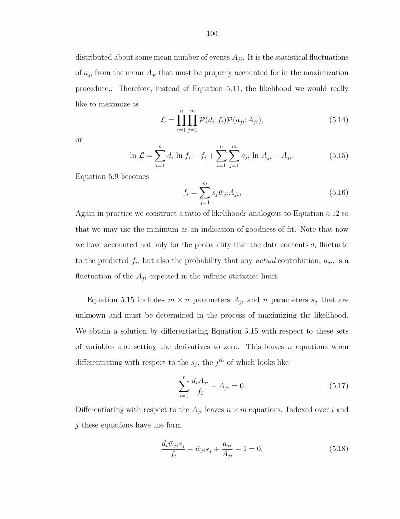
100

distributed about some mean number of events Aji. It is the statistical fluctuations

of aji from the mean Aji that must be properly accounted for in the maximization

procedure.. Therefore, instead of Equation 5.11, the likelihood we would really

like to maximize is

L =n∏

i=1

m∏j=1

P(di; fi)P(aji;Aji), (5.14)

or

ln L =n∑

i=1

di ln fi − fi +n∑

i=1

m∑j=1

aji ln Aji − Aji. (5.15)

Equation 5.9 becomes

fi =m∑

j=1

sjwjiAji, (5.16)

Again in practice we construct a ratio of likelihoods analogous to Equation 5.12 so

that we may use the minimum as an indication of goodness of fit. Note that now

we have accounted not only for the probability that the data contents di fluctuate

to the predicted fi, but also the probability that any actual contribution, aji, is a

fluctuation of the Aji expected in the infinite statistics limit.

Equation 5.15 includes m × n parameters Aji and n parameters sj that are

unknown and must be determined in the process of maximizing the likelihood.

We obtain a solution by differentiating Equation 5.15 with respect to these sets

of variables and setting the derivatives to zero. This leaves n equations when

differentiating with respect to the sj, the jth of which looks like

n∑i=1

diAji

fi

− Aji = 0. (5.17)

Differentiating with respect to the Aji leaves n×m equations. Indexed over i and

j these equations have the form

diwjisj

fi

− wjisj +aji

Aji

− 1 = 0. (5.18)

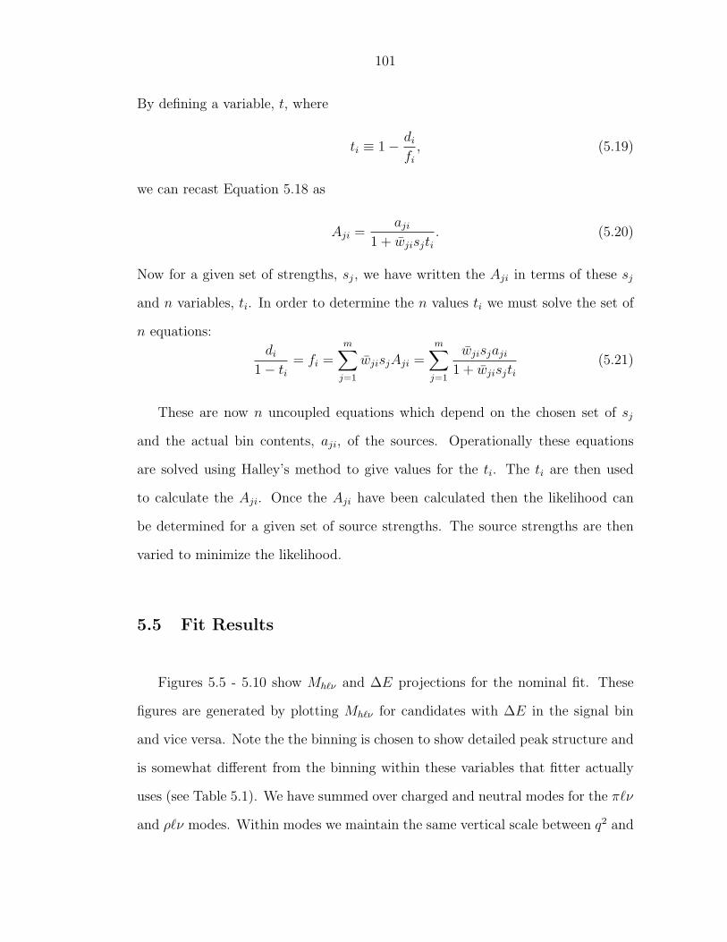
101

By defining a variable, t, where

ti ≡ 1− di

fi

, (5.19)

we can recast Equation 5.18 as

Aji =aji

1 + wjisjti. (5.20)

Now for a given set of strengths, sj, we have written the Aji in terms of these sj

and n variables, ti. In order to determine the n values ti we must solve the set of

n equations:

di

1− ti= fi =

m∑j=1

wjisjAji =m∑

j=1

wjisjaji

1 + wjisjti(5.21)

These are now n uncoupled equations which depend on the chosen set of sj

and the actual bin contents, aji, of the sources. Operationally these equations

are solved using Halley’s method to give values for the ti. The ti are then used

to calculate the Aji. Once the Aji have been calculated then the likelihood can

be determined for a given set of source strengths. The source strengths are then

varied to minimize the likelihood.

5.5 Fit Results

Figures 5.5 - 5.10 show Mh`ν and ∆E projections for the nominal fit. These

figures are generated by plotting Mh`ν for candidates with ∆E in the signal bin

and vice versa. Note the the binning is chosen to show detailed peak structure and

is somewhat different from the binning within these variables that fitter actually

uses (see Table 5.1). We have summed over charged and neutral modes for the π`ν

and ρ`ν modes. Within modes we maintain the same vertical scale between q2 and

102

Table 5.6: A summary of the central values for the exclusive branching fractionsfor B0 → π−`+ν obtained in the nominal fit. The errors shown are statistical only.

q2 [GeV 2]∫

dΓdq2dq

2/ΓTotal[10−4]

q2 < 2 0.12± 0.072 < q2 < 8 0.26± 0.078 < q2 < 16 0.54± 0.08

16 < q2 0.40± 0.07Total 1.32±0.15

cos θWl bins to demonstrate the distribution of both the signal and the background

in these variables.

The nominal fit converges with −2 ln λ equal to 391 for 392 - 21 degrees of

freedom. Recall that we fit explicity for the π±`ν and ρ±`ν yields. Given this

yield, Yπ/ρ`ν , we can obtain the branching fraction, averaged over lepton species,

as

B(B0 → π−/ρ−`+ν) =Yπ/ρ`ν

4f00NΥ(4S)

, (5.22)

where f00 is the fraction of neutral B mesons produced at the Υ(4S). The factor

four comes from a factor of two to convert NΥ(4S) to NB and another factor of

two to average over electrons and muons. For the η`ν mode we obtain a similar

expression:

B(B+ → η`+ν) =Yη`ν

4f+−NΥ(4S)

, (5.23)

Tables 5.6 and 5.7 summarize the branching fractions and statistical errors obtained

in the nominal fit for the π`ν and ρ`ν modes. In the η`ν mode we obtain the result:

B(B+ → η`+ν) = (0.45± 0.25)× 10−4.

In order to test that our fit properly models the shape of the various vari-

ables used in the candidate selection algorithm we plot these variables with the

fit components superimposed. The values obtained in the nominal fit are used to

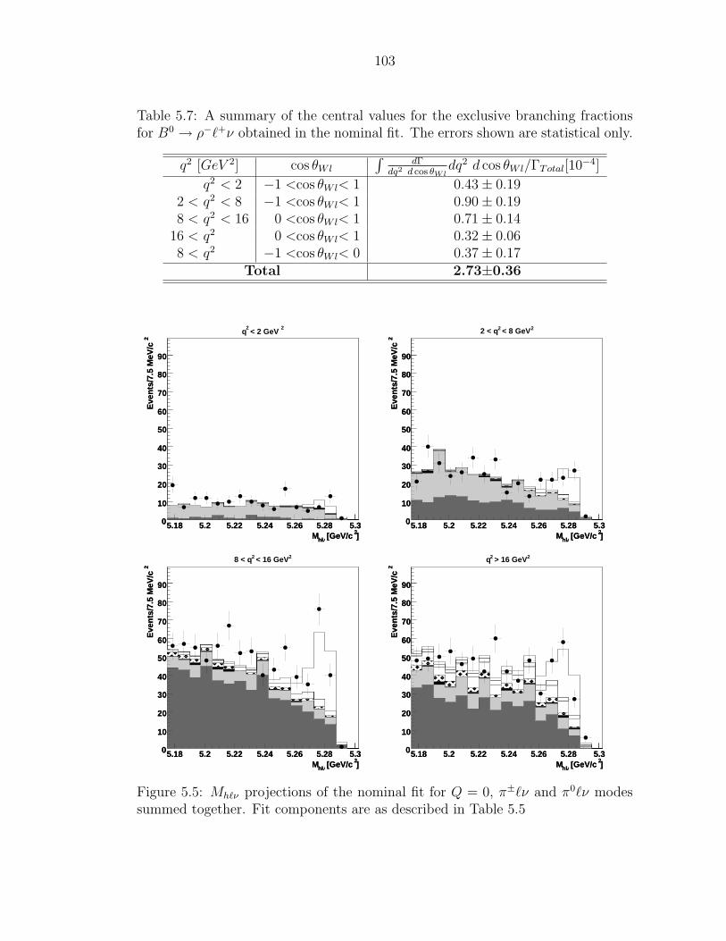
103

Table 5.7: A summary of the central values for the exclusive branching fractionsfor B0 → ρ−`+ν obtained in the nominal fit. The errors shown are statistical only.

q2 [GeV 2] cos θWl

∫dΓ

dq2 d cos θWldq2 d cos θWl/ΓTotal[10−4]

q2 < 2 −1 <cos θWl< 1 0.43± 0.192 < q2 < 8 −1 <cos θWl< 1 0.90± 0.198 < q2 < 16 0 <cos θWl< 1 0.71± 0.14

16 < q2 0 <cos θWl< 1 0.32± 0.068 < q2 −1 <cos θWl< 0 0.37± 0.17

Total 2.73±0.36

]2 [GeV/cνhlM5.18 5.2 5.22 5.24 5.26 5.28 5.3

2E

ven

ts/7

.5 M

eV/c

0

10

20

30

40

50

60

70

80

90

]2 [GeV/cνhlM5.18 5.2 5.22 5.24 5.26 5.28 5.3

2E

ven

ts/7

.5 M

eV/c

0

10

20

30

40

50

60

70

80

90

2 < 2 GeV

2q

]2 [GeV/cνhlM5.18 5.2 5.22 5.24 5.26 5.28 5.3

2E

ven

ts/7

.5 M

eV/c

0

10

20

30

40

50

60

70

80

90

]2 [GeV/cνhlM5.18 5.2 5.22 5.24 5.26 5.28 5.3

2E

ven

ts/7

.5 M

eV/c

0

10

20

30

40

50

60

70

80

90

2 < 8 GeV22 < q

]2 [GeV/cνhlM5.18 5.2 5.22 5.24 5.26 5.28 5.3

2E

ven

ts/7

.5 M

eV/c

0

10

20

30

40

50

60

70

80

90

]2 [GeV/cνhlM5.18 5.2 5.22 5.24 5.26 5.28 5.3

2E

ven

ts/7

.5 M

eV/c

0

10

20

30

40

50

60

70

80

90

2 < 16 GeV28 < q

]2 [GeV/cνhlM5.18 5.2 5.22 5.24 5.26 5.28 5.3

2E

ven

ts/7

.5 M

eV/c

0

10

20

30

40

50

60

70

80

90

]2 [GeV/cνhlM5.18 5.2 5.22 5.24 5.26 5.28 5.3

2E

ven

ts/7

.5 M

eV/c

0

10

20

30

40

50

60

70

80

90

2 > 16 GeV2 q

Figure 5.5: Mh`ν projections of the nominal fit for Q = 0, π±`ν and π0`ν modessummed together. Fit components are as described in Table 5.5

104

E [GeV]∆-0.6 -0.4 -0.2 0 0.2 0.4 0.6

Eve

nts

/100

MeV

0

10

20

30

40

50

60

70

80

E [GeV]∆-0.6 -0.4 -0.2 0 0.2 0.4 0.6

Eve

nts

/100

MeV

0

10

20

30

40

50

60

70

80

2 < 2 GeV

2q

E [GeV]∆-0.6 -0.4 -0.2 0 0.2 0.4 0.6

Eve

nts

/100

MeV

0

10

20

30

40

50

60

70

80

E [GeV]∆-0.6 -0.4 -0.2 0 0.2 0.4 0.6

Eve

nts

/100

MeV

0

10

20

30

40

50

60

70

80

2 < 8 GeV22 < q

E [GeV]∆-0.6 -0.4 -0.2 0 0.2 0.4 0.6

Eve

nts

/100

MeV

0

10

20

30

40

50

60

70

80

E [GeV]∆-0.6 -0.4 -0.2 0 0.2 0.4 0.6

Eve

nts

/100

MeV

0

10

20

30

40

50

60

70

80

2 < 16 GeV28 < q

E [GeV]∆-0.6 -0.4 -0.2 0 0.2 0.4 0.6

Eve

nts

/100

MeV

0

10

20

30

40

50

60

70

80

E [GeV]∆-0.6 -0.4 -0.2 0 0.2 0.4 0.6

Eve

nts

/100

MeV

0

10

20

30

40

50

60

70

80

2 > 16 GeV2 q

Figure 5.6: ∆E projections of the nominal fit for Q = 0, π±`ν and π0`ν modessummed together. Fit components are as described in Table 5.5

105

]2 [GeV/cνhlM5.18 5.2 5.22 5.24 5.26 5.28 5.3

2E

ven

ts/7

.5 M

eV/c

0

10

20

30

40

50

60

70

80

90

]2 [GeV/cνhlM5.18 5.2 5.22 5.24 5.26 5.28 5.3

2E

ven

ts/7

.5 M

eV/c

0

10

20

30

40

50

60

70

80

90

2 < 2 GeV

2q

]2 [GeV/cνhlM5.18 5.2 5.22 5.24 5.26 5.28 5.3

2E

ven

ts/7

.5 M

eV/c

0

10

20

30

40

50

60

70

80

90

]2 [GeV/cνhlM5.18 5.2 5.22 5.24 5.26 5.28 5.3

2E

ven

ts/7

.5 M

eV/c

0

10

20

30

40

50

60

70

80

90

2 < 8 GeV22 < q

]2 [GeV/cνhlM5.18 5.2 5.22 5.24 5.26 5.28 5.3

2E

ven

ts/7

.5 M

eV/c

0

10

20

30

40

50

60

70

80

90

]2 [GeV/cνhlM5.18 5.2 5.22 5.24 5.26 5.28 5.3

2E

ven

ts/7

.5 M

eV/c

0

10

20

30

40

50

60

70

80

90

2 < 16 GeV28 < q

]2 [GeV/cνhlM5.18 5.2 5.22 5.24 5.26 5.28 5.3

2E

ven

ts/7

.5 M

eV/c

0

10

20

30

40

50

60

70

80

90

]2 [GeV/cνhlM5.18 5.2 5.22 5.24 5.26 5.28 5.3

2E

ven

ts/7

.5 M

eV/c

0

10

20

30

40

50

60

70

80

90

2 > 16 GeV2 q

Figure 5.7: Mh`ν projections of the nominal fit for |Q| = 1, π±`ν and π0`ν modessummed together. Fit components are as described in Table 5.5

106

E [GeV]∆-0.6 -0.4 -0.2 0 0.2 0.4 0.6

Eve

nts

/100

MeV

0

10

20

30

40

50

60

70

80

E [GeV]∆-0.6 -0.4 -0.2 0 0.2 0.4 0.6

Eve

nts

/100

MeV

0

10

20

30

40

50

60

70

80

2 < 2 GeV

2q

E [GeV]∆-0.6 -0.4 -0.2 0 0.2 0.4 0.6

Eve

nts

/100

MeV

0

10

20

30

40

50

60

70

80

E [GeV]∆-0.6 -0.4 -0.2 0 0.2 0.4 0.6

Eve

nts

/100

MeV

0

10

20

30

40

50

60

70

80

2 < 8 GeV22 < q

E [GeV]∆-0.6 -0.4 -0.2 0 0.2 0.4 0.6

Eve

nts

/100

MeV

0

10

20

30

40

50

60

70

80

E [GeV]∆-0.6 -0.4 -0.2 0 0.2 0.4 0.6

Eve

nts

/100

MeV

0

10

20

30

40

50

60

70

80

2 < 16 GeV28 < q

E [GeV]∆-0.6 -0.4 -0.2 0 0.2 0.4 0.6

Eve

nts

/100

MeV

0

10

20

30

40

50

60

70

80

E [GeV]∆-0.6 -0.4 -0.2 0 0.2 0.4 0.6

Eve

nts

/100

MeV

0

10

20

30

40

50

60

70

80

2 > 16 GeV2 q

Figure 5.8: ∆E projections of the nominal fit for |Q| = 1, π±`ν and π0`ν modessummed together. Fit components are as described in Table 5.5

107

]2 [GeV/cνhlM5.18 5.2 5.22 5.24 5.26 5.28 5.3

2E

ven

ts/7

.5 M

eV/c

0

20

40

60

80

100

120

140

160

]2 [GeV/cνhlM5.18 5.2 5.22 5.24 5.26 5.28 5.3

2E

ven

ts/7

.5 M

eV/c

0

20

40

60

80

100

120

140

160

< 1Wlθ and -1 < cos2

< 2 GeV2

q

]2 [GeV/cνhlM5.18 5.2 5.22 5.24 5.26 5.28 5.3

2E

ven

ts/7

.5 M

eV/c

0

20

40

60

80

100

120

140

160

]2 [GeV/cνhlM5.18 5.2 5.22 5.24 5.26 5.28 5.3

2E

ven

ts/7

.5 M

eV/c

0

20

40

60

80

100

120

140

160


< 8 GeV2

2 < q

]2 [GeV/cνhlM5.18 5.2 5.22 5.24 5.26 5.28 5.3

2E

ven

ts/7

.5 M

eV/c

0

20

40

60

80

100

120

140

160

]2 [GeV/cνhlM5.18 5.2 5.22 5.24 5.26 5.28 5.3

2E

ven

ts/7

.5 M

eV/c

0

20

40

60

80

100

120

140

160

< 1Wlθand 0 < cos2

< 16 GeV2

8 < q

]2 [GeV/cνhlM5.18 5.2 5.22 5.24 5.26 5.28 5.3

2E

ven

ts/7

.5 M

eV/c

0

20

40

60

80

100

120

140

160

]2 [GeV/cνhlM5.18 5.2 5.22 5.24 5.26 5.28 5.3

2E

ven

ts/7

.5 M

eV/c

0

20

40

60

80

100

120

140

160

< 1Wlθand 0 < cos2

> 16 GeV2

q

]2 [GeV/cνhlM5.18 5.2 5.22 5.24 5.26 5.28 5.3

2E

ven

ts/7

.5 M

eV/c

0

20

40

60

80

100

120

140

160

]2 [GeV/cνhlM5.18 5.2 5.22 5.24 5.26 5.28 5.3

2E

ven

ts/7

.5 M

eV/c

0

20

40

60

80

100

120

140

160


> 8 GeV2

q

Figure 5.9: Mh`ν projections of the nominal fit for Q = 0, ρ±`ν and ρ0`ν modessummed together. Fit components are as described in Table 5.5

108

E [GeV]∆-0.6 -0.4 -0.2 0 0.2 0.4 0.6

Eve

nts

/100

MeV

0

20

40

60

80

100

120

140

160

180

200

220

E [GeV]∆-0.6 -0.4 -0.2 0 0.2 0.4 0.6

Eve

nts

/100

MeV

0

20

40

60

80

100

120

140

160

180

200

220 < 1Wlθ and -1 < cos

2 < 2 GeV

2q

E [GeV]∆-0.6 -0.4 -0.2 0 0.2 0.4 0.6

Eve

nts

/100

MeV

0

20

40

60

80

100

120

140

160

180

200

220

E [GeV]∆-0.6 -0.4 -0.2 0 0.2 0.4 0.6

Eve

nts

/100

MeV

0

20

40

60

80

100

120

140

160

180

200

220 < 1Wlθ and -1 < cos

2 < 8 GeV

22 < q

E [GeV]∆-0.6 -0.4 -0.2 0 0.2 0.4 0.6

Eve

nts

/100

MeV

0

20

40

60

80

100

120

140

160

180

200

220

E [GeV]∆-0.6 -0.4 -0.2 0 0.2 0.4 0.6

Eve

nts

/100

MeV

0

20

40

60

80

100

120

140

160

180

200

220 < 1Wlθand 0 < cos

2 < 16 GeV

28 < q

E [GeV]∆-0.6 -0.4 -0.2 0 0.2 0.4 0.6

Eve

nts

/100

MeV

0

20

40

60

80

100

120

140

160

180

200

220

E [GeV]∆-0.6 -0.4 -0.2 0 0.2 0.4 0.6

Eve

nts

/100

MeV

0

20

40

60

80

100

120

140

160

180

200

220 < 1Wlθand 0 < cos

2 > 16 GeV

2 q

E [GeV]∆-0.6 -0.4 -0.2 0 0.2 0.4 0.6

Eve

nts

/100

MeV

0

20

40

60

80

100

120

140

160

180

200

220

E [GeV]∆-0.6 -0.4 -0.2 0 0.2 0.4 0.6

Eve

nts

/100

MeV

0

20

40

60

80

100

120

140

160

180

200

220 < 0Wlθ and -1 < cos

2 > 8 GeV

2q

Figure 5.10: ∆E projections of the nominal fit for Q = 0, ρ±`ν and ρ0`ν modessummed together. Fit components are as described in Table 5.5

109

[GeV/c]leptonp0.8 1 1.2 1.4 1.6 1.8 2 2.2 2.4 2.6 2.8

Eve

nts

/100

MeV

/c

0

10

20

30

40

50

[GeV/c]leptonp0.8 1 1.2 1.4 1.6 1.8 2 2.2 2.4 2.6 2.8

Eve

nts

/100

MeV

/c

0

10

20

30

40

50

[GeV/c]leptonp0.8 1 1.2 1.4 1.6 1.8 2 2.2 2.4 2.6 2.8

Eve

nts

/100

MeV

/c

0

20

40

60

80

100

[GeV/c]leptonp0.8 1 1.2 1.4 1.6 1.8 2 2.2 2.4 2.6 2.8

Eve

nts

/100

MeV

/c

0

20

40

60

80

100

Figure 5.11: Lepton momentum projections of the nominal fit for Q = 0, π±`νand π0`ν (left) and ρ±`ν and ρ0`ν (right). The data have been summed over q2

and cos θWl.

normalize the fit components.

Figure 5.11 shows the lepton momentum projections for both π`ν and ρ`ν.

As expected, the signal lepton spectrum for ρ`ν is noticeably harder than that

for π`ν. The agreement between the data and the sum of the fit components

gives us confidence in the overall fit quality and our in ability to model the lepton

momentum distribution of the fit components.

Figures 5.12 and 5.13 show the projections of cos θWl and the invariant mass of

the two pions, Mππ, used to construct the ρ candidate for the ρ`ν modes. Again,

the agreement between data and the sum of the fit components is encouraging.

In the cos θWl variable the signal peaks near one and the b → c background is

concentrated in the area where cos θWl is less than zero as expected. The Mππ

projection shows a nice peak in the signal component at the ρ mass. The peak in

the highest bin is due to B → D(∗)`ν backgrounds where the D → Kπ decay is

identified as a ρ→ ππ decay. Recall that only the three bins about the ρ mass are

110

Wlθcos -1 -0.8 -0.6 -0.4 -0.2 0 0.2 0.4 0.6 0.8 1

Eve

nts

/0.1

0

20

40

60

80

100

Wlθcos -1 -0.8 -0.6 -0.4 -0.2 0 0.2 0.4 0.6 0.8 1

Eve

nts

/0.1

0

20

40

60

80

100

Figure 5.12: The cos θWl projectionof the nominal fit, summed over q2,for the ρ0`ν and ρ±`ν modes.

]2 [GeV/cππM0.4 0.6 0.8 1 1.2 1.4 1.6 1.8

2E

ven

ts/1

90 M

eV/c

0

100

200

300

400

500

600

700

800

]2 [GeV/cππM0.4 0.6 0.8 1 1.2 1.4 1.6 1.8

2E

ven

ts/1

90 M

eV/c

0

100

200

300

400

500

600

700

800

Figure 5.13: The projection of thetwo-pion invariant mass of the ρcandidates summed over q2 andcos θWl. The normalization of thefit components is determined fromthe nominal fit.

used in the fit.

The agreement shown above for various projections of the fit indicates that

the simulation and fit components model the shapes observed in the data. The

following chapter will evaluate the quality of this modeling in detail and assess the

systematic errors on the results due to uncertainties present in the Monte Carlo

and other inputs to the analysis algorithm.

Chapter 6

Systematic Uncertainties

The motivation behind evaluating a systematic error due to the uncertainty

in a given aspect of the analysis is to ask oneself how the result would change if

that aspect was different. These uncertainties can enter into the anlalysis in many

ways, for example, in detector simulation, theoretical calculations, or even errors

on other experimental results that are used the analysis. In this spirit we repeat

the entire analysis multiple times changing each uncertain aspect individually to

assess the impact of a given systematic uncertainty on the final result.

Wherever possible we have attempted to remove statistical fluctuations that

may enter as a result of repeating the analysis. For example, in Monte Carlo

electron identification we rely on random numbers coupled with data measured

efficiencies to get the same identification efficiency in data as in Monte Carlo. When

repeating the analysis for the sake of evaluation systematic errors we “freeze” this

and other aspects of the analysis that depend on random numbers.

In all cases throughout this chapter I will quote errors in percentage deviation

from the nominal results stated in the pervious chapter. We assess the error on

the total rate for a particular exclusive channel independently of the error on the

individual bins in q2 or cos θWl. Frequently the impact on the total measured rate

will be smaller than the impact on the bins due to correlated changes among the

bins.

111

112

6.1 Systematic Uncertainties in Neutrino Reconstruction

Neutrino reconstruction relies on our ability to reconstruct and identify every

particle produced in a single collision. Since we are using Monte Carlo shapes in the

Mh`ν/∆E plane to fit the data, it is necessary that all aspects of the Monte Calro,

e.g. resolution, efficiency, etc., be the same as it is in data to avoid systematic

bias.

Following the lead of the previous analysis [37] we are cautious not to underes-

timate our experimental systematic errors due to false cancellation. If we degrade

the simulated resolution of the neutrino the simulated efficiency will drop. How-

ever, the fitted signal yield will also drop because the simulated signal bin now

has a smaller fraction of signal events due to the degraded resolution on the neu-

trino. The lower raw yield combined with the lower efficiency can produce the

same efficiency corrected yield and thereby negate the systematic error in neutrino

resolution. Certainly this effect is “real” to some extent, but in cases where large

cancellation occurs we do not trust that our simulation models this cancellation

properly. In cases where the change in fit yield and efficiency have the same sign,

i.e. there is some cancellation, we add an additional√

2/3 of the magnitude of

the cancellation, which is the minimum of the change in efficiency or yield. In

other words, we assign an error on the canceling parts equal to one-third of their

magnitude and add these errors in quadrature. The fraction one-third is purely an

estimate, but is most likely conservative as there is a real cancellation effect.

Systematic errors due to neutrino reconstruction are summarized in Table 6.1

and are discussed in detail below. As expected, these systematic errors together

tend to dominate the systematic error on the rate in most bins.

113

6.1.1 Track Efficiency and Resolution

In order to assess our susceptibility to systematic errors in the track finding

efficiency of the Monte Carlo we repeat the analysis randomly dropping some

fraction of the tracks. For CLEO II and II.V Berger notes [49] that systematic error

on the Monte Carlo efficiency for track finding is 2.6% for tracks with momenta

less than 250 MeV/c and 0.5% otherwise. The systematic error on low momentum

tracking in CLEO III has not been extensively studied therefore, like Briere et

al. [50], we use a conservative 5% error on low momentum tracks. The track finding

error for high momentum tracks in CLEO III is taken to 0.5% in agreement with

studies by Liu and Gao [51]. The analysis is repeated simultaneously dropping 2.6%

(5%) of low momentum tracks for CLEO II/II.V (III) and 0.5% of high momentum

tracks. This makes the conservative assumption that the tracking systematic error

is fully correlated between CLEO II/II.V and CLEO III. The deviations from the

nominal result are listed in Table 6.1 in the Track Efficiency row.

We explore potential biases due to errors in simulating track resolution by

degrading the resolution in our Monte Carlo simulation. It is important to stress

that errors in the result only arise when the resolution is different in Monte Carlo

and reconstructed data. The absolute resolution is irrelevant. We choose to reset

the momentum, ~precon, of each reconstruction track to

~precon → ~precon + δ~p, (6.1)

where

δ~p ≡ α (~precon − ~ptrue) . (6.2)

In Monte Carlo we determine the true momentum, ~ptrue, by looking at the generator

level information. This process increases the error on the reconstructed track by

114

some amount α. For CLEO II and II.V we choose α to be 10%. CLEO III studies

of the D width in the decay of D → Kπ indicate that the Monte Carlo resolution

should be smeared by 40% to broaden the width such that it agrees with data.

The analysis is repeated smearing every Monte Carlo track by 10% (40%) in CLEO

II/II.V (III), and the deviation from the nominal results are listed in the Track

Resolution row of Table 6.1.

6.1.2 Shower Efficiency and Resolution

Shower reconstruction systematic errors are evaluated in a similar fashion to

the tracking errors. Gritsan has limited the shower finding systematic error in

CLEO II/II.V to 1.6% [52]. In CLEO III the shower finding systematic error is

reduced to 1%. The analysis is again repeated while randomly dropping 1.6% (1%)

of the showers in CLEO II/II.V (III) and the resulting systematic errors are noted

in the Shower Efficiency row of Table 6.1.

Just as we did with tracks, the procedure outlined in Equations 6.1 and 6.2 is

repeated with showers. We degrade all showers by 10%. Previous CLEO II/II.V

studies and recent work by Muramatsu and Skwarnicki [53] indicate that actual

resolution discrepancy is at or below the 10% level. The impact of this systematic

error on the analysis is listed in the Shower Resolution row of Table 6.1.

6.1.3 Splitoff Simulation and Rejection

Potential systematic errors arise in the ability of the Monte Carlo to properly

model so-called hadronic splitoff showers. In order to evaluate this error clean

γγ → K0SK

0S events with each K0

S decaying into π+π− were compared in data and

115

Monte Carlo [54]. Based on the comparison of the multiplicity of hadronic showers

in these events we add on average 0.03 showers per hadron to each event to ex-

plore systematic discrepancies between data and Monte Carlo. These showers are

distributed uniformly throughout the detector and are drawn from a determined

spectrum of splitoff showers which is concentrated at lower energies. Errors as-

sociated with this modeling mistake are shown in the Splitoff Simulation row of

Table 6.1.

A additional systematic error in rejecting splitoff showers may arise in the vari-

ables used as inputs to the neural net that is used to identify the splitoff showers.

In order to assess the impact of this systematic error we bias our neural net output

in Monte Carlo. The bias procedure systematically pushes the neural net output

for tagged photons in the “splitoff direction” and simultaneously pushes the out-

put for showers not tagged to photons in the “photon direction” thus degrading

the effectiveness of the algorithm. Meyer provides an extensive discussion on the

implementation and effect of the bias [45]. Systematic changes in the result are

listed in the Splitoff Algorithm row of Table 6.1.

6.1.4 Particle Identification

As mentioned earlier the ability to identify charged particles directly affects the

missing energy resolution in neutrino reconstruction. We smear the time of flight

(dE/dx) significance in CLEO II/II.V by 12

(14) of the intrinsic resolution in the

more pion-like direction. The degree of the smearing in each of these variables is

thought to be a conservative estimate of the potential systematic error in detector

information [55].

116

In CLEO III we find that degrading the proton and kaon probabilities based

on detector information (PsD in Section 4.2.2) by 70% of themselves and turning

off the production fraction weighting, i.e. setting PsD → 1, we produce systematic

changes in the kaon and proton identification efficiencies at the 5% level. Studies

using similar particle identification algorithms have limited systematic errors in

CLEO III to less than 5% [56].

To determine the total impact due to systematic errors in particle identification

we simultaneously degrade time of flight and dE/dx information in CLEO II/II.V

and we degrade PKD and Pp

D by 70% of themselves in our CLEO III particle identi-

fication algorithm. The resulting error is shown in the Particle Identification row

of Table 6.1.

6.1.5 K0L Production and Energy Deposition

A substantial portion of the “missed particles” that inflate the resolution on the

reconstructed neutrino are K0L’s. We noted in Section 5.3.1 that by counting K0

S’s

in B decay we infer that theK0L multiplicity in the Monte Carlo should be increased

by a factor of 1.072 [38]. The error on this determination is 1%, therefore we vary

the weight up and down by 1% and average the absolute values of the deviation

for a total error due to incorrect K0L production in the Monte Carlo.

We also probe the effect of systematically increasing the energy deposited by

K0L’s in the calorimeter by increasing the energy of showers tagged to generator-

level K0L’s by 20%. This systematic error has a very minor impact on the result

and is listed as K0L Energy Deposition in Table 6.1.

117

6.1.6 Secondary Lepton Spectrum

As noted in Section 5.3.1 we correct the spectrum of secondary leptons based

on the measurements of the inclusive B → D∗X spectrum [39] and the electron

spectrum in inclusive semileptonic charm decay [40]. This spectrum is correlated

with the spectrum of secondary neutrinos and therefore impacts neutrino resolu-

tion. We determine the allowable minimum and maximum weights as a function

of momentum given the errors of these two measurements. We repeat the analysis

using each of these sets of weights and then average the absolute values of the

deviations to determine the potential systematic error due to uncertainties in the

secondary lepton spectrum.

6.2 Additional Sources of Systematic Error

Aside from those systematic errors that directly impact the resolution of the

reconstructed neutrino, there are a variety of other systematic errors to be consid-

ered. We attempt to isolate vulnerabilities in our analysis and or fit procedure due

to dependancy on uncertain theoretical or experimental information. Again we

proceed in the sprit of repeating the analysis and varying each unknown quantity

independently to explore systematic effects.

6.2.1 Continuum Suppression

The continuum smoothing algorithm outlined in Section 5.3.2 relies on our

ability to model the bias introduced in the Mh`ν/∆E plane by the continuum

suppression cuts. Using an appropriate Monte Carlo sample the bias parameters,

118

Tab

le6.

1:A

sum

mar

yof

the

syst

emat

icer

rors

asso

ciat

edw

ith

neu

trin

ore

const

ruct

ion.

The

bin

num

ber

sar

eas

list

edin

Tab

les

5.2

and

5.3

onpag

es80

and

83.

Err

ors

from

diff

eren

tso

urc

esar

eas

sum

edto

be

unco

rrel

ated

.T

he

bot

tom

row

show

sth

equad

ratu

re-s

um

ofth

eer

rors

.

δB(B

0→

π−`+ν)

[%]

δB(B

0→

ρ−`+ν)

[%]

Sys

tem

atic

Err

orSou

rce

12

34

Tot

al1

23

45

Tot

alTra

ckE

ffici

ency

4.0

4.9

2.2

4.2

1.8

6.5

7.6

3.4

6.4

1.8

3.3

Tra

ckR

esol

ution

1.5

1.7

1.6

1.3

1.4

9.2

13.8

2.4

4.1

40.5

1.9

Show

erE

ffici

ency

2.0

3.5

6.4

3.5

4.6

5.0

7.3

7.0

7.0

23.6

2.1

Show

erR

esol

uti

on2.

34.

83.

31.

83.

07.

56.

96.

33.

01.

85.

5Splito

ffSim

ula

tion

3.6

1.4

2.4

1.7

1.6

7.0

8.1

2.0

0.2

26.5

1.0

Splito

ffR

ejec

tion

2.9

2.9

1.4

1.7

0.6

8.1

2.2

4.9

0.3

3.1

2.9

Par

ticl

eId

enti

fica

tion

0.6

2.2

0.7

4.3

1.1

7.3

12.6

1.1

3.6

18.0

2.3

K0 L

Pro

duct

ion

0.2

0.1

0.3

0.2

0.2

0.6

0.9

0.1

0.3

4.0

0.2

K0 L

Ener

gyD

epos

itio

n0.

00.

00.

20.

20.

12.

42.

60.

60.

68.

30.

8Sec

ondar

yLep

ton

Spec

trum

0.5

1.2

0.4

0.3

0.1

6.7

0.6

0.5

0.2

2.7

1.5

Tota

lN

eutr

ino

Reco

nst

ruct

ion

Syst

em

ati

cErr

or

7.0

8.9

8.3

7.7

6.3

20.7

24.2

11.6

11.4

57.7

8.2

119

α and β, in Equation 5.4 are determined through a fit. We determine one pair

of bias parameters and its error for each set of Fisher weights. This produces 26

pairs or 42 total parameters that are independent and uncorrelated. To assess

the uncertainty due to the error on these bias parameters, we vary one of the

parameters up and down one sigma as determined from the fit. We average the

absolute value of the deviation from the nominal value and repeat the process

for the remaining 45 parameters. The average deviations for each parameter are

added in quadrature to produce the total systematic error due to our continuum

suppression algorithm as listed in Table 6.2. Note that the dependance of the

magnitude of this error on bin is as expected: low q2 bins that contain large

continuum backgrounds are affected most.

6.2.2 B → Xc`ν

In the generic B decay simulation we have already applied weights to correct

the generator level branching fractions of B → D`ν, B → D∗`ν, B → D∗∗`ν, and

non-resonant B → Xc`ν to agree with the previous CLEO result [41]. To evaluate

sensitivity to this correction we vary each of these four rates up and down one

sigma as reported in [41]. The magnitudes of the deviation are averaged for each

variation to produce a systematic error for each of the four rates.

In addition we consider variations of the B → D∗`ν form factor as it is the

dominant B → Xc`ν decay and a likely background. Following the example of

Lipeles [42] we simultaneously vary the slope and curvature parameters, ρ2 and

c, of the Isgur-Wise function to span the set of allowed values. Specifically our

nominal fit uses (ρ2, c2) = (1.20, 0.7) and we vary these up to (1.51,1.39) and down

to (0.88,0.0). The simultaneous motion accounts for correlations in the parameters.

120

We average the magnitude of the deviation and combine this in quadrature with

the four variations of the branching fractions outlined in the previous paragraph.

The full systematic uncertainty due to B → Xc`ν decays is shown in Table 6.2.

Again, as expected, maximum impact is seen at low q2 and especially in the ρ`ν

mode where B → Xc`ν backgrounds are large.

6.2.3 Other B → Xu`ν

As noted in Section 5.3.5 we use a hybrid exclusive-inclusive Monte Carlo to

model other B → Xu`ν decays aside from the signal decay. We generate two addi-

tional sets of the Monte Carlo varying the heavy quark expansion parameters up

and down as allowed by the CLEO B → Xsγ photon spectrum measurement [46].

We take the average magnitude of the deviation as the systematic error due to the

modeling of the inclusive lepton spectrum in the decay.

Additionally the magnitude of the other B → Xu`ν component in the fit is

fixed by the BaBar endpoint measurement [47] as outlined in Section 5.3.5. We

vary the endpoint rate within the errors allowed by the BaBar measurement and

combine the average magnitude of the deviation in quadrature with the shape error

described above to produce a total systematic error due to potential mis-modeling

of the other B → Xu`ν background.

6.2.4 Lepton Identification and Fake Leptons

Recall that electron identification in Monte Carlo is done by measuring electron

efficiencies in data and then reproducing this efficiency in Monte Carlo using true

generated electrons and random numbers. The statistical errors on the data mea-

121

surement of the efficiency dominate the systematic error on due to electron iden-

tification. Past studies have shown that muon identification efficiency in CLEO II

and II.V Monte Carlo agrees with data at the 2% level. The study discussed in

Appendix A shows that on average 2% errors or better can be achieved by applying

a weight to correct the efficiency which is applied in our nominal fit. All aspects of

our lepton identification algorithm are shown to be reproduced in Monte Carlo or

are artificially mocked up in Monte Carlo with accuracies at or below 2%. Since

we have one signal lepton per decay we simply take 2% as the systematic error on

the efficiency and therefore branching fraction due to lepton identification.

We rely on measurements of the rates for hadrons faking leptons in two ways in

our fit and therefore should consider potential systematic error due to statistical

errors in the measurement of the fake rates. First, we use the fake rates to produce

a fit contribution that is from BB events in which the only lepton in the event is

a fake signal lepton. As can be seen from the fit projections this contribution is

minute and is dominated by the statistical error on the on-resonance minus off-

resonance subtraction procedure. This statistical error is already accounted for

in the fit; therefore, we neglect potential systematic errors in the production of

this fit component. Secondly the data-measured fake rates are used to veto events

in Monte Carlo that have an additional lepton which arises from a hadron faking

a lepton. A systematic error in the fake rate would affect the efficiency of the

multiple-lepton veto and therefore affect the signal efficiency. We systematically

lower the fake rates by 12

to probe the sensitivity of our result to the data-measured

fake rates. The deviations are listed in the Fake Leptons row of Table 6.2.

122

6.2.5 π0 Identification

The CLEO III Monte Carlo is known to overestimate the π0 efficiency. This

is likely due to improper modeling of the pre-shower of the photon in the RICH

detector or other material in front of the calorimeter. In data this pre-shower

degrades the shower shape and produces an efficiency loss. Cassel et al. measure

the discrepancy between data and Monte Carlo to be 4% [57]. Therefore in our

nominal fit we apply a weight of 0.96 to CLEO III Monte Carlo signal decays that

contain a π0 in the final state. Note that π0 finding is only used in the process of

reconstructing signal decays. To explore the effect of systematic errors in CLEO

III π0 identification, we set the weight used in the fit to one, effectively removing

the correction that exists in the nominal fit.

6.2.6 Number of Υ → BB Events

Based on luminosity, cross section, and event shape studies the error on the

number of BB events in CLEO II + II.V is taken to be 2%. It is further assumed

that the error is strongly correlated between the CLEO II and II.V data set such

that the ratio the number BB events in each is well known. In order to determine

the number of BB events in the CLEO III data set Alexander et al. measure the

ratio of B → Dπ in CLEO II + II.V and in CLEO III [58] to an accuracy of 8%.

Since we lock the relative ratios of CLEO II, II.V, and III in the fit and each of

these detector configurations has a different reconstruction efficiency, we decide to

probe what effect the uncertainty in the II + II.V : III ratio has on the result. The

ratio is varied ±8% while keeping the total number of BB events constant and the

resulting deviation is negligible. We combine the 2% error for the number of BB

123

events in CLEO II and II.V with the 8% error on the ratio of number of BB events

in II + II.V : III to produce a total error on the number of BB events of 3.6% that

accounts for correlations between the two measurements. This translates directly

to a 3.6% systematic error on the branching fractions from the uncertainty in the

total number of Υ → BB events.

6.2.7 τB+/τB0 and f+−/f00

The fixed relative strengths of the charged and neutral rates are sensitive to

both the lifetime and production ratios of charged and neutral B mesons through

Equation 5.8. We vary both the lifetime and production fraction ratios indepen-

dently within the error bars produced by the Heavy Flavor Averaging Group [44].

Additionally the error on f+−/f00 affects our calculation of the total number B0

mesons produced through Equation 5.22. This effect combined with correlated

effect on the charged/neutral constraint in the fit is listed in Table 6.2. The inde-

pendent effect of the error on τB+/τB0 is listed separately.

6.3 Dependance on Form Factors

Past attempts at measurement of the B → π`ν and B → ρ`ν rates have

been plagued by the theoretical uncertainty regarding the form factors for these

decays. As noted before, experimental efficiency is not uniform across the allowed

kinematic space for these decays and the experimentalist must rely on theoretical

calculations to extrapolate what is measured to the full rate. Our choice of binning

in the q2 and cos θWl variables allows a rate measurement with minimal dependance

on theoretically calculated form factors.

124

Tab

le6.

2:A

sum

mar

yof

the

exper

imen

talsy

stem

atic

erro

rs.

The

bin

num

ber

sar

eas

list

edin

Tab

les

5.2

and

5.3

onpag

es80

and

83.

Err

ors

from

diff

eren

tso

urc

esar

eas

sum

edto

be

unco

rrel

ated

.N

eutr

ino

reco

nst

ruct

ion

syst

emat

icer

rors

are

copie

ddir

ectl

yfr

omth

eto

tals

sum

mar

ized

inTab

le6.

1.

δB(B

0→

π−`+ν)

[%]

δB(B

0→

ρ−`+ν)

[%]

Sys

tem

atic

Err

orSou

rce

12

34

Tot

al1

23

45

Tot

alN

eutr

ino

Rec

onst

ruct

ion

7.0

8.9

8.3

7.7

6.3

20.7

24.2

11.6

11.4

57.7

8.2

Con

tinuum

Suppre

ssio

n9.

82.

90.

91.

01.

19.

31.

81.

41.

33.

41.

5B→

Xc`ν

3.9

4.0

1.2

0.9

1.5

20.8

12.2

2.3

2.3

13.7

5.9

Oth

erB→

Xu`ν

2.0

1.4

2.0

5.0

2.3

5.6

2.5

7.6

4.9

16.6

3.1

Fak

eLep

tons

4.7

1.2

2.3

0.5

1.8

3.1

2.6

1.6

1.0

5.4

1.2

Lep

ton

Iden

tifica

tion

2.0

2.0

2.0

2.0

2.0

2.0

2.0

2.0

2.0

2.0

2.0

π0

Iden

tifica

tion

0.4

0.2

0.2

0.2

0.1

1.0

0.9

1.4

0.9

3.3

1.4

Num

ber

ofΥ→

BB

3.6

3.6

3.6

3.6

3.6

3.6

3.6

3.6

3.6

3.6

3.6

τ B+/τ

B0

0.5

0.3

0.4

0.4

0.4

0.7

0.7

0.6

0.8

0.4

0.7

f +−/f

00

0.5

0.8

0.7

0.7

0.7

0.1

0.0

0.2

0.2

0.7

0.1

Tota

lExperi

menta

lSyst

em

ati

cErr

or

14.3

11.1

9.9

10.2

8.3

31.7

27.7

14.9

13.4

62.2

11.6

125

To evaluate the dependance on the form factors, we choose a set of calculations

that span the extreme range of theoretical results. We then re-weight our signal

Monte Carlo according to each of these form factor calculations to evaluate the

systematic error of the form factor on the rate measurement. We vary the B → π`ν

and B → ρ`ν independently as any change can affect all measured rates in the

fit due to cross feed. We take the systematic error on rate due to the B → π`ν

form factor to be 1.7 times the RMS of the set of rates produced with the form

factor variations and likewise for B → ρ`ν rates. We inflate the RMS by a factor

of 1.7 to account for potential variations of the internal parameters of any the

calculated form factors. This inflation factor is purely an empirical result derived

from exploring variations within individual models and was used in the previous

CLEO analysis [37].

6.3.1 The B → π`ν Form Factor

The unquenched lattice QCD result of Shigemitsu et al. [16] are used in the

nominal fit. We probe the allowed space of form factors by also repeating the anal-

ysis using the calculations of Ball and Zwicky [14], Scora and Isgur (ISGW2) [11],

and Feldmann and Kroll [13] for the B → π`ν form factor. We use the nominal

Ball and Zwicky result for the B → ρ`ν form factor [15] throughout this study.

The variation in q2 dependance of the rate from these calculations is illustrated in

Figure 6.1. We take the RMS of the results in each bin for the four calculations

inflated by 70% of itself as the systematic error due to the B → π`ν form factor

uncertainty.

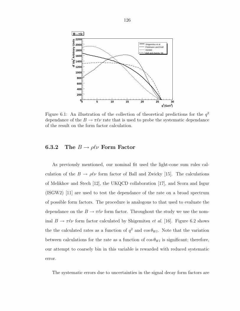
126

]2 [GeV2q

0 5 10 15 20 25 30

Arb

itra

ry U

nit

s2

/dq

Γd

0

200

400

600

800

1000

1200

1400

1600

1800

2000

2200

Shigemitsu et al.Feldmann and KrollISGW2Ball and Zwicky ’04

ν lπ→B

Figure 6.1: An illustration of the collection of theoretical predictions for the q2

dependance of the B → π`ν rate that is used to probe the systematic dependanceof the result on the form factor calculation.

6.3.2 The B → ρ`ν Form Factor

As previously mentioned, our nominal fit used the light-cone sum rules cal-

culation of the B → ρ`ν form factor of Ball and Zwicky [15]. The calculations

of Melikhov and Stech [12], the UKQCD collaboration [17], and Scora and Isgur

(ISGW2) [11] are used to test the dependance of the rate on a broad spectrum

of possible form factors. The procedure is analogous to that used to evaluate the

dependance on the B → π`ν form factor. Throughout the study we use the nom-

inal B → π`ν form factor calculated by Shigemitsu et al. [16]. Figure 6.2 shows

the the calculated rates as a function of q2 and cos θWl. Note that the variation

between calculations for the rate as a function of cos θWl is significant; therefore,

our attempt to coarsely bin in this variable is rewarded with reduced systematic

error.

The systematic errors due to uncertainties in the signal decay form factors are

127

]2 [GeV2q

0 5 10 15 20 25

Arb

itra

ry U

nit

s2

/dq

Γd

0

200

400

600

800

1000

1200

1400

1600

1800

2000

2200

2400Ball and Zwicky ’04

Melikhov and Stech

ISGW2

UKQCD

ν lρ→B

Wlθcos -1 -0.8 -0.6 -0.4 -0.2 0 0.2 0.4 0.6 0.8 1

Arb

itra

ry U

nit

sW

lθ

/dco

s Γd

0

200

400

600

800

1000

1200

1400

1600

1800

2000

2200

2400Ball and Zwicky ’04

Melikhov and Stech

ISGW2

UKQCD

ν lρ→B

Figure 6.2: Shown are the predicted rate as a function of q2 (left) and cos θWl

(right) for the set of form factor calculations used to study the systematic error onthe rate due to the uncertainty in the B → ρ`ν form factor.

Table 6.3: The systematic errors associated with the individual B → π`ν andB → ρ`ν form factor uncertainties are listed below. The bin numbers are as listedin Tables 5.2 and 5.3 on pages 80 and 83.

δB (B0 → π−`+ν) [%] δB (B0 → ρ−`+ν) [%]Form Factor 1 2 3 4 Total 1 2 3 4 5 TotalB → π`ν 1.6 0.6 0.7 3.5 1.0 0.4 0.5 1.1 0.4 3.4 0.6B → ρ`ν 0.5 0.8 1.5 1.2 1.0 2.8 5.7 1.4 2.0 9.6 1.4

summarized in Table 6.3. Dramatic improvements over the previous CLEO result

have been made in minimizing the effect of the B → ρ`ν form factor uncertainty.

In fact the error bar on the total B → ρ`ν rate due to form factor uncertainties

has been reduced by an order of magnitude.

Chapter 7

Summary and Conclusions

I have presented a measurement of the of the B0 → π−`ν and B0 → ρ−`ν

rates in bins of the momentum transfer variable, q2, and the lepton decay angle,

θWl. The rates were measured using 15.4 million Υ(4S) → BB events recorded

with the CLEO II, II.V, and III detectors. The analysis technique utilizes neutrino

reconstruction in order to exclusively reconstruct the products of the semileptonic

B decay. A binned likelihood fit is used to simultaneously extract the rates for the

various decay modes and kinematic variable bins. Careful systematic studies were

carried out to assess both the experimental and theoretical systematic errors.

7.1 Summary of the Rates

In order to produce a measurement with appropriate errors we combine the

central values and statistical error bars determined in the fit in Chapter 5 with the

fractional systematic errors that were studied in Chapter 6. Historically results

have depended strongly on the choice of form factor used to analyze and interpret

the data. In order to emphasize this, the systematic error is often separated show to

independently show the portion due to form factor uncertainty. This dependance,

studied in the latter portion of the previous chapter, has been greatly reduced in

this analysis. To highlight this I will combine the uncertainties due to B → ρ`ν

and B → π`ν form factors but still list this uncertainty separately from other

systematic errors.

Tables 7.1 and 7.2 summarize the rate measurements and the relevant statistical

128

129

Table 7.1: A summary of the exclusive branching fractions for B0 → π−`+ν ob-tained in this analysis. The errors shown are statistical, systematic, and formfactor associated respectively.

q2 [GeV 2]∫

dΓdq2dq

2/ΓTotal[10−4]

q2 < 2 0.12± 0.07± 0.02± 0.002 < q2 < 8 0.26± 0.07± 0.03± 0.008 < q2 < 16 0.54± 0.08± 0.05± 0.01

16 < q2 0.40± 0.07± 0.04± 0.01Total 1.32 ± 0.15 ± 0.11 ± 0.02

Table 7.2: A summary of the exclusive branching fractions for B0 → ρ−`+ν ob-tained in this analysis. The errors shown are statistical, systematic, and formfactor associated respectively.

q2 [GeV 2] cos θWl

∫dΓ

dq2 d cos θWldq2 d cos θWl/ΓTotal[10−4]

q2 < 2 −1 <cos θWl< 1 0.43± 0.19± 0.13± 0.012 < q2 < 8 −1 <cos θWl< 1 0.90± 0.19± 0.25± 0.058 < q2 < 16 0 <cos θWl< 1 0.71± 0.14± 0.11± 0.01

16 < q2 0 <cos θWl< 1 0.32± 0.06± 0.05± 0.018 < q2 −1 <cos θWl< 0 0.37± 0.17± 0.23± 0.04

Total 2.73 ± 0.36 ± 0.32 ± 0.04

and systematic errors. In most bins, the total error is dominated by the statistical

component. With the lowered lepton momentum cut and fitting of data with

cos θWl < 0 in the B → ρ`ν modes, we have managed to produce measurements

for both modes that have a residual dependance on the decay form factors that is

at or below the 2% level.

7.2 Comparison with Other Measurements

We can compare our results for the total B0 → π−`ν and B0 → ρ−`ν branching

fractions with other independent results from the BaBar and Belle collaborations.

130

-4x 100.5 1 1.5 2

Belle SL Tag (hep-ex/0408145)

BaBar SL Tag (CKM 2005)

-recon (CKM 2005)νBaBar

This Result

)ν+l-π → 0BF( B

-4x 102 3 4

CLEO (PRD 61, 052001 2000)

BaBar (PRL 90, 181801 2003)

Belle SL Tag (hep-ex/0408145)

-recon (CKM 2005)νBaBar

This Result

)ν+l-ρ → 0BF( B

Figure 7.1: The current world results for B0 → π−`ν (left) and B0 → ρ−`ν (right)branching fractions are shown. Error bars are statistical, experimental systematic,and form factor associated. The world average and one sigma error is shown. Allof the errors are assumed to be uncorrelated in the computation of the average.

Figure 7.1 shows a comparison of the various independent measurements of the

B0 → π−`ν and B0 → ρ−`ν branching fractions. The world average and one stan-

dard deviation error bar, assuming uncorrelated errors among the measurements,

are shown. Not only do the results presented in this analysis agree remarkably

with other measurements, they are also the most precise measurements to date of

the total branching fractions. Furthermore as can be seen in Figure 7.1 for the

first time a result for the total B0 → ρ−`ν branching fraction has been produced

with virtually no residual dependance on the B0 → ρ−`ν form factor.

7.3 Final Thoughts

We have measured the B0 → π−`ν and B0 → ρ−`ν to better than the 15%

and 18% level respectively, the best measurements available to date. Equally as

important, we have successfully decoupled the experimental measurement from the

131

underlying theoretical uncertainty in the decay form factor. While the precision in

the individual q2 or cos θWl bins in this analysis is not high enough to effectively

discriminate between the current form factor calculations, there are other routes

to verification of form factors, such as high-statistics semileptonic D decay studies

currently underway at CLEO. When the theoretical community produces verified,

precise form factor calculations, either of the two branching fractions presented in

this work can be used on its own to produce a sub-10% measurement for |Vub|.

We have therefore contributed an important experimental result that, when used

in concert with other independent results and appropriate theoretical input, is

capable pushing precision tests of the Standard Model to new extremes.

Appendix A

CLEO III Muon Identification Efficiency

and Fake Rates

In general, we identify muons in two categories. The first category, so-called

“counting muons,” is subject to much looser requirements and used only when

vetoing an event that has multiple leptons. The second category called “signal

muons” is a smaller subset of these counting muons that is used for reconstructing

signal B → Xµν decays. The details of the identification algorithm are presented

in Section 4.2.1. Here we examine the discrepancies between data and MC and

make a measurement of the rate at which hadrons fakes muons.

A.1 Muon Efficiency

In order to check that our Monte Carlo simulation appropriately models the

muon efficiency in data we measure the efficiency using radiative µ-pair events and

compare this efficiency with what is observed for generated muons in the Monte

Carlo.

A.1.1 True Muon Sample in Data

We need to select events of the type e+e− → µ+µ−γ, where the γ is radiated

by the µ that we wish to study. We do so by looking at events that have strictly

two tracks and only one shower with energy > 1 GeV . We then require that

132

133

[GeV/c]trackp0 1 2 3 4 5 6

[G

eV/c

]γp

0

1

2

3

4

5

6

0

20

40

60

80

100

120

140

160

180

200

PairsµSingle Tag Radidative

trackφ-3 -2 -1 0 1 2 3

0

100

200

300

400

500

600

700

800

900

True Muons

Figure A.1: (left) pγ vs. ptrack with selection criteria described in the text; (right)φtrack: no sign of cosmic ray contamination is visible

one of the tracks, call it µtag, satisfy the signal muon requirements above and

also have ptag > 5.0 GeV/c. We can then plot pγ vs. ptrack, where ptrack is the

momentum of the other track in the event. This is shown in Figure A.1. The

vertical band at ptrack ≈ 5.2 GeV/c is most likely due to pure µ − pair events

where the interactions of one muon with the calorimeter produced the additional

shower. For ptrack < 3.0 GeV/c (the region we wish to study), we can isolate true

muons by requiring |pγ + ptrack − 5.3 GeV/c| < 0.7 GeV/c. Finally we require

that the track under study have |cos θ| < 0.65; therefore, we measure the efficiency

within this fiducial volume. To verify that this sample is not contaminated by

cosmic rays we plot φtrack also in Figure A.1 – no structure is observed.

A.1.2 True Muon Sample in Monte Carlo

Obtaining a sample of true muons in Monte Carlo is much simpler. We re-

quire that the generator-level particle be a muon and that it be matched to a

134

reconstructed track. In addition we require that this track be within the fiducial

volume, |cos θ| < 0.65.

A.1.3 Divisions Among Run Ranges

Throughout this study we will define “CLEO III Data” as being data sets 6

through 14 inclusive. The corresponding “CLEO III Monte Carlo” is generated

for all of those data sets and roughly in the appropriate proportions. We will use

signal, b → ulν MC, as it provides a supply of leptons with momenta out to 2.8

GeV/c.

Midway through the CLEO III running a bug in the online muon sparsification

code was discovered and repaired. Fixing this bug resulted in a noticeable change

in efficiency; therefore, it is worthwhile to to compare efficiencies with and without

the sparsification bug. All runs before run 116853 have the bug – from run 116853

onward the bug is fixed. The effect of the bug on the efficiency in data is show in

Figure A.2.

A.1.4 Efficiency Comparison

Figure A.3 shows a comparison of the data and Monte Carlo efficiencies for

muons as a function of momentum. From this plot one can conclude that the

efficiency in Monte Carlo seems to be systematically too low by 1-2%. Figure A.4

shows a similar data/Monte Carlo comparison independently for runs before and

after the sparsification fix. While the efficiency for runs taken with the bug is well

modeled in the Monte Carlo, it seems that the Monte Carlo failed to reproduce

the efficiency gain in data once the bug was fixed.

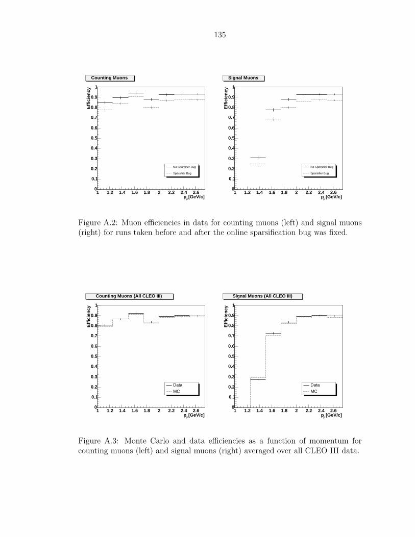
135

[GeV/c]µp1 1.2 1.4 1.6 1.8 2 2.2 2.4 2.6

Eff

icie

ncy

0

0.1

0.2

0.3

0.4

0.5

0.6

0.7

0.8

0.9

1

No Sparsifier Bug

Sparsifier Bug

Counting Muons

[GeV/c]µp1 1.2 1.4 1.6 1.8 2 2.2 2.4 2.6

Eff

icie

ncy

0

0.1

0.2

0.3

0.4

0.5

0.6

0.7

0.8

0.9

1

No Sparsifier Bug

Sparsifier Bug

Signal Muons

Figure A.2: Muon efficiencies in data for counting muons (left) and signal muons(right) for runs taken before and after the online sparsification bug was fixed.

[GeV/c]µp1 1.2 1.4 1.6 1.8 2 2.2 2.4 2.6

Eff

icie

ncy

0

0.1

0.2

0.3

0.4

0.5

0.6

0.7

0.8

0.9

1

Data

MC

Counting Muons (All CLEO III)

[GeV/c]µp1 1.2 1.4 1.6 1.8 2 2.2 2.4 2.6

Eff

icie

ncy

0

0.1

0.2

0.3

0.4

0.5

0.6

0.7

0.8

0.9

1

Data

MC

Signal Muons (All CLEO III)

Figure A.3: Monte Carlo and data efficiencies as a function of momentum forcounting muons (left) and signal muons (right) averaged over all CLEO III data.

136

[GeV/c]µp1 1.2 1.4 1.6 1.8 2 2.2 2.4 2.6

Eff

icie

ncy

0

0.1

0.2

0.3

0.4

0.5

0.6

0.7

0.8

0.9

1

Data

MC

Counting Muons (Sparsifier Bug)

[GeV/c]µp1 1.2 1.4 1.6 1.8 2 2.2 2.4 2.6

Eff

icie

ncy

0

0.1

0.2

0.3

0.4

0.5

0.6

0.7

0.8

0.9

1

Data

MC

Signal Muons (Sparsifier Bug)

[GeV/c]µp1 1.2 1.4 1.6 1.8 2 2.2 2.4 2.6

Eff

icie

ncy

0

0.1

0.2

0.3

0.4

0.5

0.6

0.7

0.8

0.9

1

Data

MC

Counting Muons (No Sparsifier Bug)

[GeV/c]µp1 1.2 1.4 1.6 1.8 2 2.2 2.4 2.6

Eff

icie

ncy

0

0.1

0.2

0.3

0.4

0.5

0.6

0.7

0.8

0.9

1

Data

MC

Signal Muons (No Sparsifier Bug)

Figure A.4: Monte Carlo and data efficiencies for counting muons (left) and signalmuons (right) for runs taken with the sparsification bug (top) and after the bugfix (bottom)

137

A.1.5 Efficiency Correction

In order to correct the data/Monte Carlo discrepancy we choose to apply a

weight to each true muon in the Monte Carlo that is reconstructed as a signal or

counting muon. Since the signal muons are strictly a subset of the counting muons

we divide the sample into two parts: one for signal muons and one for counting

but not signal muons. Note that this division only exists for muons with momenta

less than 1.75 GeV/c. We further divide those samples in to two sets depending

on whether the run was taken before or after the sparsification bug fix. The result

is four sets of momentum dependent weights, one of which will be used for each

Monte Carlo muon. These weights are given in the table below:

Run < 116853 Run ≥ 116853

pµ [GeV/c] Signal Counting Signal Counting

1.00-1.25 – 0.981±0.018 – 1.065±0.017

1.25-1.50 0.858±0.049 1.033±0.028 1.044±0.060 1.016±0.033

1.50-1.75 0.987±0.021 1.032±0.062 1.061±0.020 0.881±0.071

1.75-2.00 0.989±0.015 – 1.044±0.014 –

2.00-2.25 0.997±0.011 – 1.035±0.009 –

2.25-2.50 1.009±0.009 – 1.016±0.008 –

2.50-2.75 1.007±0.010 – 1.029±0.009 –

A.2 Muon Fake Rates

We also need to measure the probability that a true pion, kaon, or proton will

be reconstructed as a muon. Here we will make a data-based measurement and

use this measurement directly in our analysis Monte Carlo instead of relying on

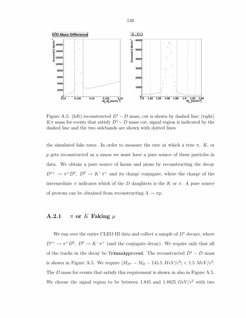
138

]2 [GeV/cD-M*DM

0.14 0.145 0.15 0.155 0.16

2E

ven

ts/0

.5 M

eV/c

0

2000

4000

6000

8000

10000

12000

14000

16000

/D Mass Difference*D

]2 [GeV/cπKM1.8 1.82 1.84 1.86 1.88 1.9 1.92 1.94

2E

ven

ts/2

.5 M

eV/c

0

1000

2000

3000

4000

5000

6000

π K→D

Figure A.5: (left) reconstructed D∗−D mass, cut is shown by dashed line; (right)Kπ mass for events that satisfy D∗−D mass cut, signal region is indicated by thedashed line and the two sidebands are shown with dotted lines

the simulated fake rates. In order to measure the rate at which a true π, K, or

p gets reconstructed as a muon we must have a pure source of these particles in

data. We obtain a pure source of kaons and pions by reconstructing the decay

D∗+ → π+D0, D0 → K−π+ and its charge conjugate, where the charge of the

intermediate π indicates which of the D daughters is the K or π. A pure source

of protons can be obtained from reconstructing Λ → πp.

A.2.1 π or K Faking µ

We run over the entire CLEO III data and collect a sample of D∗ decays, where

D∗+ → π+D0, D0 → K−π+ (and the conjugate decay). We require only that all

of the tracks in the decay be TrkmanApproved. The reconstructed D∗ − D mass

is shown in Figure A.5. We require |MD∗ −MD − 145.5 MeV/c2| < 1.5 MeV/c2.

The D mass for events that satisfy this requirement is shown in also in Figure A.5.

We choose the signal region to be between 1.845 and 1.8825 GeV/c2 with two

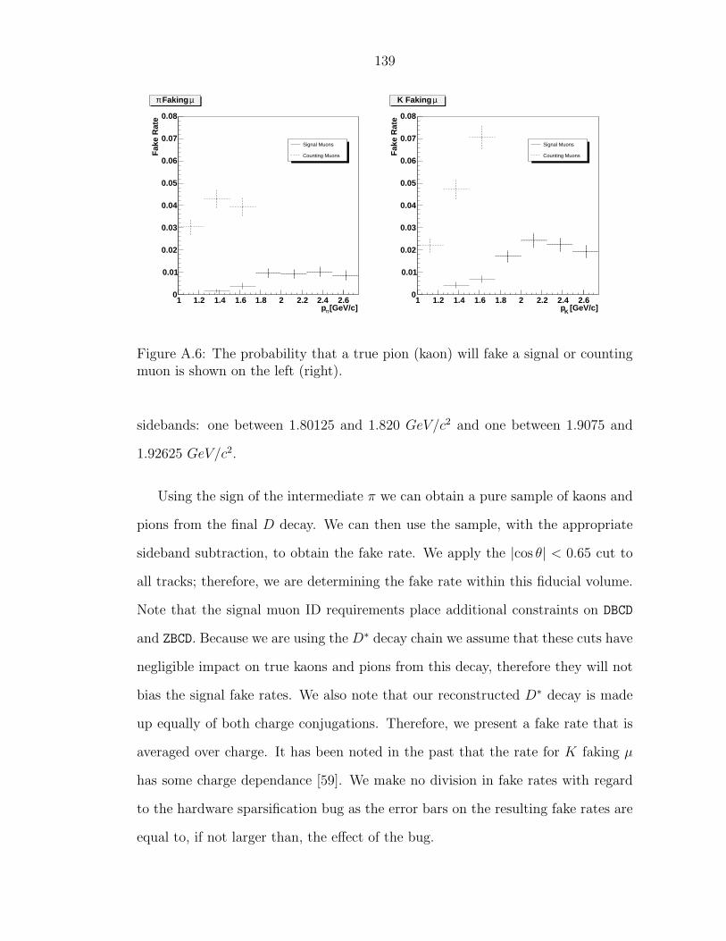
139

[GeV/c]πp1 1.2 1.4 1.6 1.8 2 2.2 2.4 2.6

Fak

e R

ate

0

0.01

0.02

0.03

0.04

0.05

0.06

0.07

0.08

Signal Muons

Counting Muons

µ Faking π

[GeV/c]Kp1 1.2 1.4 1.6 1.8 2 2.2 2.4 2.6

Fak

e R

ate

0

0.01

0.02

0.03

0.04

0.05

0.06

0.07

0.08

Signal Muons

Counting Muons

µK Faking

Figure A.6: The probability that a true pion (kaon) will fake a signal or countingmuon is shown on the left (right).

sidebands: one between 1.80125 and 1.820 GeV/c2 and one between 1.9075 and

1.92625 GeV/c2.

Using the sign of the intermediate π we can obtain a pure sample of kaons and

pions from the final D decay. We can then use the sample, with the appropriate

sideband subtraction, to obtain the fake rate. We apply the |cos θ| < 0.65 cut to

all tracks; therefore, we are determining the fake rate within this fiducial volume.

Note that the signal muon ID requirements place additional constraints on DBCD

and ZBCD. Because we are using the D∗ decay chain we assume that these cuts have

negligible impact on true kaons and pions from this decay, therefore they will not

bias the signal fake rates. We also note that our reconstructed D∗ decay is made

up equally of both charge conjugations. Therefore, we present a fake rate that is

averaged over charge. It has been noted in the past that the rate for K faking µ

has some charge dependance [59]. We make no division in fake rates with regard

to the hardware sparsification bug as the error bars on the resulting fake rates are

equal to, if not larger than, the effect of the bug.

140

The fake rates for π and K faking µ are present in the table below and in

Figure A.6. For tracks with momenta above 1.75 GeV/c the counting fake rate is

equivalent to the signal fake rate.

π faking µ[%] K faking µ [%]

p [GeV/c] Signal Counting Signal Counting

1.00-1.25 0.0 3.05±0.34 0.0 2.20±0.31

1.25-1.50 0.16±0.08 4.29±0.40 0.42±0.13 4.75±0.44

1.50-1.75 0.39±0.12 3.93±0.38 0.69±0.16 7.07±0.52

1.75-2.00 0.97±0.20 – 1.72±0.26 –

2.00-2.25 0.94±0.20 – 2.45±0.31 –

2.25-2.50 1.02±0.22 – 2.24±0.31 –

2.50-2.75 0.87±0.22 – 1.94±0.30 –

A.2.2 p Faking µ

In order to obtain a pure sample of protons we reconstruct the decay Λ → πp.

We require that both of the tracks be TrkmanApproved and also we required that

the vertex of the Λ be displaced from the beam spot by at least 10 cm. The

reconstructed πp mass is shown in Figure A.7. We define the signal region from

1.1135 to 1.1185 GeV/c2 and two sidebands: one from 1.105-1.1075 GeV/c2 and

one from 1.1245-1.127 GeV/c2.

The displaced vertex requirement will bias tracks against our signal selection

criteria. In addition, the efficiency for TrkmanApproved tracks drops as vertices

become more displaced from the beam spot. Because of these systematic effects,

and because low level of precision needed for the measured proton fake rate, we

will assume fake rates for signal muons are the same as those for counting muons.

141

]2 [GeV/cπpM1.1 1.105 1.11 1.115 1.12 1.125 1.13

2E

ven

ts/0

.5 M

eV

/c

0

5000

10000

15000

20000

25000

30000

35000

π p →Λ

Figure A.7: reconstructed pπ in-variant mass, the signal (sideband)region is indicated by dashed (dot-ted) lines

[GeV/c]pp1 1.2 1.4 1.6 1.8 2 2.2 2.4 2.6

Fak

e R

ate

0

0.01

0.02

0.03

0.04

0.05

0.06

0.07

0.08

µp Faking

Figure A.8: probability that a pro-ton will fake a counting muon – er-ror bars are statistical only

As seen above, this is most likely a conservative over-estimate of the signal fake

rate. In addition we will assign a conservative 100% error to the measured proton

fake rates to account for systematic errors in the measurement. The fake rates are

shown in the table below and in Figure A.8.

p [GeV/c] p faking µ [%]

1.00-1.25 0.18

1.25-1.50 0.32

1.50-1.75 1.36

1.75-2.00 0.57

2.00-2.25 0.84

2.25-2.50 0.77

2.50-2.75 0.26

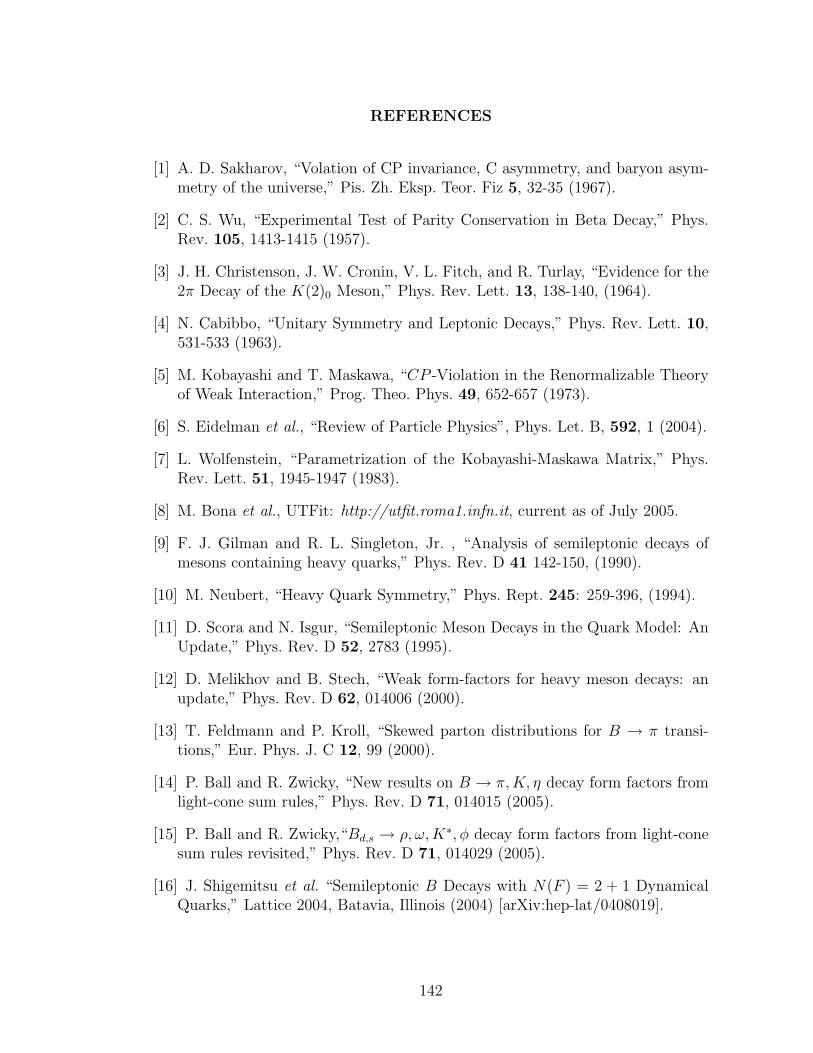
REFERENCES

[1] A. D. Sakharov, “Volation of CP invariance, C asymmetry, and baryon asym-metry of the universe,” Pis. Zh. Eksp. Teor. Fiz 5, 32-35 (1967).

[2] C. S. Wu, “Experimental Test of Parity Conservation in Beta Decay,” Phys.Rev. 105, 1413-1415 (1957).

[3] J. H. Christenson, J. W. Cronin, V. L. Fitch, and R. Turlay, “Evidence for the2π Decay of the K(2)0 Meson,” Phys. Rev. Lett. 13, 138-140, (1964).

[4] N. Cabibbo, “Unitary Symmetry and Leptonic Decays,” Phys. Rev. Lett. 10,531-533 (1963).

[5] M. Kobayashi and T. Maskawa, “CP -Violation in the Renormalizable Theoryof Weak Interaction,” Prog. Theo. Phys. 49, 652-657 (1973).

[6] S. Eidelman et al., “Review of Particle Physics”, Phys. Let. B, 592, 1 (2004).

[7] L. Wolfenstein, “Parametrization of the Kobayashi-Maskawa Matrix,” Phys.Rev. Lett. 51, 1945-1947 (1983).

[8] M. Bona et al., UTFit: http://utfit.roma1.infn.it, current as of July 2005.

[9] F. J. Gilman and R. L. Singleton, Jr. , “Analysis of semileptonic decays ofmesons containing heavy quarks,” Phys. Rev. D 41 142-150, (1990).

[10] M. Neubert, “Heavy Quark Symmetry,” Phys. Rept. 245: 259-396, (1994).

[11] D. Scora and N. Isgur, “Semileptonic Meson Decays in the Quark Model: AnUpdate,” Phys. Rev. D 52, 2783 (1995).

[12] D. Melikhov and B. Stech, “Weak form-factors for heavy meson decays: anupdate,” Phys. Rev. D 62, 014006 (2000).

[13] T. Feldmann and P. Kroll, “Skewed parton distributions for B → π transi-tions,” Eur. Phys. J. C 12, 99 (2000).

[14] P. Ball and R. Zwicky, “New results on B → π,K, η decay form factors fromlight-cone sum rules,” Phys. Rev. D 71, 014015 (2005).

[15] P. Ball and R. Zwicky,“Bd,s → ρ, ω,K∗, φ decay form factors from light-conesum rules revisited,” Phys. Rev. D 71, 014029 (2005).

[16] J. Shigemitsu et al. “Semileptonic B Decays with N(F ) = 2 + 1 DynamicalQuarks,” Lattice 2004, Batavia, Illinois (2004) [arXiv:hep-lat/0408019].

142

143

[17] L. Del Debbio et al. [UKQCD Collaboration], “Lattice constrainedparametrizations of form-factors for semileptonic and rare radiative B decays,”Phys. Lett. B 416, 392 (1998).

[18] F. De Fazio and M. Neubert,“B → Xu`ν lepton decay distributions to orderα(s),” JHEP 9906, 017 (1999).

[19] Y. Kubota et al., “The CLEO II Detector,” NIM A 320, 66 (1992).

[20] D. G. Cassel et al., “Design and Construction of the CLEO II Drift Chamber,”NIM A 252, 325 (1986).

[21] D. Peterson et al., “The CLEO III Drift Chamber,” NIM A 478, 142 (2002).

[22] W. Ross, “The CLEO II.V Silicon Vertex Detector,” NIM A 386, 32 (1997).

[23] R. Kass et al., “The CLEO III Silicon Vertex Detector,” NIM A 501, 32(2003).

[24] R. Mountain et al., “The CLEO III RICH Detector,” NIM A 433, 77 (1999).

[25] C. Bebek, “A Cesium Iodide Calorimeter with Photodiode Readout for CLEOII,” NIM A 265 258 (1988).

[26] S. Roberts, L. Gibbons, and E. Thorndike, “Trkman the Next Generation,The Quest for Track Quality,” CLEO CBX 96-103.

[27] T. Meyer, https://www.lns.cornell.edu/˜cleo3/development/src/SplitoffProd/Doc.

[28] S. Pappas, https://www.lns.cornell.edu/˜pappas/private/KinFit/FittingDoc.html.

[29] C. H. Wang, “Electron Identification with CLEO II,” CLEO CBX 91-52.

[30] C. S. Park, “CLEO III Rochester Electron Identification,” CLEO CBX Draftv1.3, April 2003.

[31] R. A. Fisher, “The Use of Multiple Measurements in Taxonomic Problems,”Annals of Eugenics, 7:179, 1936.

[32] F. Wurthwein and J. Alexander, “Details on Continuum Suppression as usedin the Analysis of B0 → K+π− and B0 → π+π−,” CLEO CBX 93-41.

[33] G. Fox and S. Wolfram, “Observables for the Analysis of Event Shapes ine+e− Annihilation and Other Processes,” Phys. Rev. Lett. 41, 1581 (1978).

[34] See for example Chapter 1 of An Introduction to Quantum Field Theory, byM. Peskin and D. Schroeder.

[35] R. Wang, “Measurements of the Inclusive Semileptonic Branching Franction ofB Mesons at the Υ(4S) resonance,” Ph.D. Thesis, Univ. of Minnesota, (1994).

144

[36] V. Boisvert, “A Study of Exclusive Charmless Semileptonic B Decays withthe CLEO Detector,” Ph.D. Thesis, Cornell University, (2002).

[37] S. B. Athar et al. [CLEO Collaboration], “Study of the q2 dependence ofB → π`ν and B → ρ(ω)`ν decay and extraction of |Vub|,” Phys. Rev. D 68,072003 (2003).

[38] A. Warburton, private communication.

[39] L. Gibbons et al. [CLEO Collaboration], “The inclusive decays B → DX andB → D∗X,” Phys. Rev. D 56, 3783 (1997).

[40] C. S. Park, private communication.

[41] S. E. Csorna et al. [CLEO Collaboration], “Moments of the B Meson InclusiveSemileptonic Decay Rate using Neutrino Reconstruction,” Phys. Rev. D 70,032002 (2004).

[42] E. Lipeles, “A Study of the Fully Differential Inclusive Semileptonic B MesonDecay Rate,” Ph.D. Thesis, California Institute of Technology, (2003).

[43] A. Lyon et al. “Improvement of the Determination of Vub using the b → sγPhoton Energy Spectrum,” CLEO-CBX 01-59.

[44] Heavy Flavor Averaging Group, http://www.slac.stanford.edu/xorg/hfag, Dec.2004.

[45] T. Meyer, “Limits on Weak Annihilation in Inclusive Charmless SemileptonicB Decays,” Ph.D. Thesis, Cornell Univeristy, (2005).

[46] S. Chen et al. [CLEO Collaboration], “Branching Fraction and Photon EnergySpectrum b→ sγ,” Phys. Rev. Lett. 87, 251807 (2001).

[47] B. Aubert et al. [BaBar Collaboration], “Measurement of the Inclusive Elec-tron Spectrum in Charmless Semileptonic B Decays Near the Kinematic End-point and Determination of |Vub|, International Conference on High EnergyPhysics, Beijing, Chinia, (2004) [arXiv:hep-ex/0408075].

[48] R. Barlow and C. Beeston, “Fitting Using Finite Monte Carlo Samples,”Comp.Phys.Comm. 77, 219 (1993).

[49] B. Berger, “Tracking Efficiency Studies II: Recompress Results,” CLEO CBX00-32.

[50] R. Briere et al., “Study of the Semileptonic Charm Decays: D0 → π−`+ν andD0 → K−`+ν,” CLEO CBX 04-12.

[51] F. Liu and Y. Gao, “Tracking Efficiency Systematics at CLEO III,” CLEOCBX 02-13.

145

[52] A. Gritsan, “Γ (η → 3π) /Γ (η → γγ) and η/π0/γ Systematics,” CLEO CBX99-72.

[53] H. Muramatsu and T. Skwarnicki, “Inclusive Photon Analysis in bb System,”CLEO CBX 04-24.

[54] A. Warburton, private communication.

[55] R. Briere, private communication.

[56] R. Briere et al., “SSS Report on Hadron PID in CLEO III: Skims, Studies,and Systematics,” CLEO CBX 03-37.

[57] D. Cassel et al., “Determination of Tracking, K0S, π0, and Particle Identifica-

tion Efficiencies, CLEO CBX 05-07.

[58] J. Alexander et al., “CLEO III Measurement of Rare Hadronic B Decays,”CLEO CBX 02-37.

[59] A. Bellerive, “Fake Muons Study with DPTHMU > 3,” CLEO CBX 97-59.

the differential rates of exclusive charmless semileptonic ... · the differential rates of...

Documents