the determinants of market outcomes
TRANSCRIPT

1The Determinants of Market Outcomes
A solid knowledge of both econometric and economic theory is crucial when design-ing and implementing empirical work in economics. Econometric theory providesa framework for evaluating whether data can distinguish between hypotheses ofinterest. Economic theory provides guidance and discipline in empirical investiga-tions. In this chapter, we first review the basic principles underlying the analysisof demand, supply, and pricing functions, as well as the concept and applicationof Nash equilibrium. We then review elementary oligopoly theory, which is thefoundation of many of the empirical strategies discussed in this book. Continuingto develop the foundations for high-quality empirical work, in chapter 2 we reviewthe important elements of econometrics for investigations. Following these first tworeview chapters, chapters 3–10 develop the core of the material in the book. Theconcepts reviewed in these first two introductory chapters will be familiar to all com-petition economists, but it is worthwhile reviewing them since understanding thesekey elements of economic analysis is crucial for an appropriate use of quantitativetechniques.
1.1 Demand Functions and Demand Elasticities
The analysis of demand is probably the single most important component of mostempirical exercises in antitrust investigations. It is impossible to quantify the likeli-hood or the effect of a change in firm behavior if we do not have information aboutthe potential response of its customers. Although every economist is familiar withthe shape and meaning of the demand function, we will take the time to brieflyreview the derivation of the demand and its main properties since basic conceptualerrors in its handling are not uncommon in practice. In subsequent chapters we willsee that demand functions are critical for many results in empirical work undertakenin the competition arena.
1.1.1 Demand Functions
We begin this chapter by reviewing the basic characteristics of individual demandand the derivation of aggregate demand functions.
Copyrighted Material

2 1. The Determinants of Market Outcomes
50
100
Q
P
Slope is −2
∆P
∆Q
Figure 1.1. (Inverse) demand function.
1.1.1.1 The Anatomy of a Demand Function
An individual’s demand function describes the amount of a good that a consumerwould buy as a function of variables that are thought to affect this decision such asprice Pi and often income y. Figure 1.1 presents an example of an individual lineardemand function for a homogeneous product: Qi D 50 � 0:5Pi or rather for theinverse demand function, Pi D 100 � 2Qi . More generally, we may write Qi DD.Pi ; y/.1 Inverting the demand curve to express price as a function of quantitydemanded and other variables yields the “inverse demand curve” Pi D P.Qi ; y/.Standard graphs of an individual’s demand curve plot the quantity demanded of thegood at each level of its own price and take as a given the level of income and thelevel of the prices of products that could be substitutes or complements. This meansthat along a given plotted demand curve, those variables are fixed. The slope of thedemand curve therefore indicates at any particular point by how much a consumerwould reduce (increase) the quantity purchased if the price increased (decreased)while income and any other demand drivers stayed fixed.
In the example in figure 1.1, an increase in price, �P , of €10 will decrease thedemand for the product by 5 units shown as �Q. The consumer will not purchaseany units if the price is above 100 because at that point the price is higher than thevalue that the customer assigns to the first unit of the good.
One interpretation of the inverse demand curve is that it shows the maximum pricethat a consumer is willing to pay if she wants to buy Qi units of the good. While a
1 This will be familiar from introductory microeconomics texts as the “Marshallian” demand curve(Marshall 1890).
Copyrighted Material
1.1. Demand Functions and Demand Elasticities 3
consumer may value the first unit of the good highly, her valuation of, say, the onehundredth unit will typically be lower and it is this diminishing marginal valuationwhich ensures that demand curves typically slope downward. If our consumer buysa unit only if her marginal valuation is greater than the price she must pay, then theinverse demand curve describes our consumer’s marginal valuation curve.
Given this interpretation, the inverse demand curve describes the differencebetween the customer’s valuation of each unit and the actual price paid for eachunit. We call the difference between what the consumer is willing to pay for eachunit and what he or she actually pays the consumer’s surplus available from thatunit. For concreteness, I might be willing to pay a maximum of €10 for an umbrellaif it’s raining, but may nonetheless only have to pay €5 for it, leaving me with ameasure of my benefit from buying the umbrella and avoiding getting wet, a surplusof €5. At any price Pi , we can add up the consumer surplus available on all of theunits consumed (those with marginal valuations above Pi ) and doing so providesan estimate of the total consumer surplus if the price is Pi .
In a market with homogeneous products, all products are identical and perfectlysubstitutable. In theory this results in all products having the same price, which isthe only price that determines the demand. In a market with differentiated products,products are not perfectly substitutable and prices will vary across products soldin the market. In those markets, the demand for any given product is determinedby its price and the prices of potential substitutes. In practice, markets which lookhomogeneous from a distance will in fact be differentiated to at least some degreewhen examined closely. Homogeneity may nonetheless be a reasonable modelingapproximation in many such situations.
1.1.1.2 The Contribution of Consumer Theory: Deriving Demand
Demand functions are classically derived by using the behavioral assumption thatconsumers make choices in a way that can be modeled as though they have anobjective, to maximize their utility, which they do subject to the constraint that theycannot spend more than they earn.As is well-known to all students of microeconomictheory, the existence of such a utility function describing underlying preferencesmay in turn be established under some nontrivial conditions (see, for example, Mas-Colell et al. 1995, chapter 1). Maximizing utility is equivalent to choosing the mostpreferred bundle of goods that a consumer can buy given her wealth.
More specifically, economists have modeled a customer of type .yi ; �i / as choos-ing to maximize her utility subject to the budget constraint that her total expenditurecannot be higher than her income:
Vi .p1; p2; : : : ; pJ ; yi I �i / D maxq1;q2;:::;qJ
ui .q1; q2; : : : ; qJ I �i /
subject to p1q1 C p2q2 C � � � C pJ qJ 6 yi ;
Copyrighted Material

4 1. The Determinants of Market Outcomes
where pj and qj are prices and quantities of good j , ui .q1; q2; : : : ; qJ I �i / is theutility of individual i associated with consuming this vector of quantities, yi is thedisposable income of individual i , and �i describes the individual’s preference type.In many empirical models using this framework, the “i” subscripts on the V and ufunctions will be dropped so that all differences between consumers are capturedby their type .yi ; �i /.
Setting up this problem by using a Lagrangian provides the first-order conditions
@ui .q1; q2; : : : ; qJ ; yi I �i /
@qjD �pj
()@ui .q1; q2; : : : ; qJ ; yi I �i /=@qj
pjD � for j D 1; 2; : : : ; J;
together with the budget constraint which must also be satisfied. We have a total ofJ C 1 equations in J C 1 unknowns: the J quantities and the value of the Lagrangemultiplier, �.
At the optimum, the first-order conditions describe that the Lagrange multiplieris equal to the marginal utility of income. In some cases it will be appropriate toassume a constant marginal utility of income. If so, we assume behavior is describedby a utility function with an additively separable good q1, the price of which isnormalized to 1, so that ui .q1; q2; : : : ; qJ I �i / D Qui .q2; : : : ; qJ I �i /C q1 and p1 D1. This numeraire good q1 is normally termed “money” and its inclusion provides anintuitive interpretation of the first-order conditions. In such circumstances a utility-maximizing consumer will choose a basket of products so that the marginal utilityprovided by the last euro spent on each product is the same and equal to the marginalutility of money, i.e., 1.2
More generally, the solution to the maximization problem describes the individ-ual’s demand for each good as a function of the prices of all the goods being soldand also the consumers’ income. Indexing goods by j , we can write the individual’sdemands as
qij D dij .p1; p2; : : : ; pJ Iyi I �i /; j D 1; 2; : : : ; J:
A demand function for product j incorporates not only the effect of the own priceof j on the quantity demanded but also the effect of disposable income and theprice of other products whose supply can affect the quantity of good j purchased.In figure 1.1, a change in the price of j represents a movement along the curve whilea change in income or in the price of other related goods will result in a shift orrotation of the demand curve.
2 This is called a quasi-linear demand function and gives the result because the first-order conditionfor good 1 collapses to
� D@ui .q1; q2; : : : ; qJ ; yi I �i /=@q1
p1D@ui .q1; q2; : : : ; qJ ; yi I �i /
@q1;
which is the marginal utility of a monetary unit. That in turn is equal to one.
Copyrighted Material

1.1. Demand Functions and Demand Elasticities 5
The utility generated by consumption is described by the (direct) utility function,ui , which relates the level of utility to the goods purchased and is not observed. Weknow that not all levels of consumption are possible because of the budget constraintand that the consumer will choose the bundle of goods that maximizes her utility.The indirect utility function Vi .p; yi I �i /, where p D .p1; p2; : : : ; pJ /, describesthe maximum utility a consumer can feasibly obtain at any level of the prices andincome. It turns out that the direct and indirect utility functions each can be used tofully describe the other.
In particular, the following result will turn out to be important for writing downdemand systems that we estimate.
For every indirect utility function Vi .p; yi I �i / there is a direct utility functionui .q1; q2; : : : ; qJ I �i / that represents the same preferences over goods providedthe indirect utility function satisfies some properties, namely that Vi .p; yi I �i / iscontinuous in prices and income, nonincreasing in price, nondecreasing in income,quasi-convex in .p; yi / with any one element normalized to 1 and homogeneousdegree zero in .p; yi /.
This result sounds like a purely theoretical one, but it will actually turn out to bevery useful in practice. In particular, it will allow us to retrieve the demand functionqi .pIyi I �i / without actually explicitly solving the utility-maximization problem.3
Computationally, this is an important simplification.
1.1.1.3 Aggregation and Total Market Size
Individual consumers’ demand can be aggregated to form the market aggregatedemand by adding the individual quantities demanded by each customer at anygiven price. If qij D dij .p1; p2; : : : ; pJ Iyi I �i / describes the demand for productj by individual i , then aggregate (total) demand is simply the sum across individuals:
Qj D
IXiD1
qij D
IXiD1
dij .p1; p2; : : : ; pJ ; yi I �i /; j D 1; 2; : : : ; J;
where I is the total number of people who might want to buy the good. Manypotential customers will set qij D 0 at least for some sets of prices p1; p2; : : : ; pJeven though they will have positive purchases at lower prices of some products. Insome cases, known as single “discrete choice” models, each individual will only buyat most one unit of the good and so dij .p1; p2; : : : ; pJ ; yi I �i / will be an indicatorvariable taking on the value either zero or one depending on whether individual ibuys the good or not at those prices. In such models, the total number of people
3 This result is known as a “duality” result and is often taught in university courses as a purelytheoretical equivalence result. For its very practical implications, see chapter 9, where we describe theuse of Roy’s identity to generate empirical demand systems from indirect utility functions rather thanthe direct utility formulation.
Copyrighted Material

6 1. The Determinants of Market Outcomes
who may want to buy the good is also the total potential market size. (We willdiscuss discrete choice models in more detail in chapter 9.) On the other hand, whenindividuals can buy more than one unit of the good, to establish the total potentialmarket size we need to evaluate both the total potential number of consumers andalso the total number of goods they might buy. Often the total potential number ofconsumers will be very large—perhaps many millions—and so in many econometricdemand models we will approximate the summation with an integral.
In general, total demand for product j will depend on the full distribution ofincome and consumer tastes in the population. However, under very special assump-tions, we will be able to write the aggregate market demand as a function of aggregateincome and a limited set of taste parameters only:
Qj D Dj .p1; p2; : : : ; pJ ; Y I �/;
where Y DPIiD1 yi .
For example, suppose for simplicity that �i D � for all individuals and everyindividual’s demand function is “additively separable” in the income variable sothat an individual’s demand function can be written
dij .p1; p2; : : : ; pJ ; yi I �i / D d�ij .p1; p2; : : : ; pJ I�/C jyi ;
where j is a parameter common to all individuals, then aggregate demand forproduct j will clearly only depend on aggregate income. Such a demand functionimplies that, given the prices of goods, an increase in income will have an effect ondemand that is exactly the same no matter what the level of the prices of all of thegoods in the market. Vice versa, an increase in the prices will have the same effectwhatever the level of income.4
The study of the conditions under which we can aggregate demand functionsand express them as a function of characteristics of the income distribution such asthe sum of individual incomes is called the study of aggregability.5 Lessons fromthat literature motivate the use of particular functional forms for demand systems inempirical work such as the almost ideal demand system (AIDS6). In general, whenbuilding empirical models we may well want to allow market demand to dependon other statistics from the income distribution besides just the total income. Forexample, we might think demand for a product depends on total income in thepopulation but also the variance, skewness, or kurtosis of the income distribution.Intuitively, this is fairly clear since if a population were made up of 1,000 people
4 If consumer types are heterogeneous but are not observed by researchers, then an empirical aggre-gate demand model will typically assume a parametric distribution for consumer types in a population,f� .� I�/. In that case, the aggregate demand model will depend on parameters � of the distribution ofconsumer types. We will explore such models in chapter 9.
5 For a technical discussion of the founding works, see the various papers by W. M. Gorman collectedin Gorman (1995). More recent work includes Lewbel (1989).
6An unfortunate acronym, which has led some authors to describe the model as the nearly idealdemand system (NIDS).
Copyrighted Material

1.1. Demand Functions and Demand Elasticities 7
making €1bn and everyone else making €10,000, then sales of €15,000 cars wouldbe at most 1,000. On the other hand, the same total income divided more equallycould certainly generate sales of more than 1,000. (For recent work, see, for example,Lewbel (2003) and references therein.)
1.1.2 Demand Elasticities
Elasticities in general, and demand elasticities in particular, turn out to be veryimportant for lots of areas of competition policy. The reason is that the “price elas-ticity of demand” provides us with a unit-free measure of the consumer demandresponse to a price increase.7 The way in which demand changes when prices goup will evidently be important for firms when setting prices to maximize profitsand that fact makes demand elasticities an essential part of, for example, mergersimulation models.
1.1.2.1 Definition
The most useful measurement of the consumer sensitivity to changes in prices is the“own-price” elasticity of demand. As the name suggests, the own-price elasticity ofdemand measures the sensitivity of demand to a change in the good’s own-price andis defined as
�jj D%�Qj%�Pj
D100.�Qj =Qj /
100.�Pj =Pj /:
The demand elasticity expresses the percentage change in quantity that results froma 1% change in prices. Alfred Marshall introduced elasticities to economics andnoted that one of their great properties is that they are unit free, unlike prices whichare measured in currency (e.g., euros per unit) and quantities (sales volumes) whichare measured in a unit of quantity per period, e.g., kilograms per year. In our examplein figure 1.1 the demand elasticity for a price increase of 10 leading to a quantitydecrease of 5 from the baseline position, where P D 60 and Q D 20, is �jj D.�5=20/=.10=60/ D �1:5.
For very small variations in prices, the demand elasticity can be expressed by usingthe slope of the demand curve times the ratio of prices to quantities. A mathematicalresult establishes that this can also be written as the derivative with respect to thelogarithm of price of the log transformation of demand curve:
�jj DPj
Qj
@Qj
@PjD@ lnQj@ lnPj
:
7 The term “elasticity” is sometimes used as shorthand for “price elasticity of demand,” which in turnis shorthand for “the elasticity of demand with respect to prices.” We will sometimes resort to the sameshorthand terminology since the full form is unwieldy. That said, we do so with the caveat that, sinceelasticities can be both “with respect to” and “of” anything, the terms elasticity or “demand elasticity” areinherently ambiguous and therefore somewhat dangerous. We will, for example, talk about the elasticityof costs with respect to output.
Copyrighted Material

8 1. The Determinants of Market Outcomes
Demand at a particular price point is considered “elastic” when the elasticity isbigger than 1 in absolute value.An elastic demand implies that the change in quantityfollowing a price increase will be larger in percentage terms so that revenues for aseller will fall all else equal.An inelastic demand at a particular price level refers to anelasticity of less than 1 in absolute value and means that a seller could raise revenuesby increasing the price provided again that everything else remained the same. Theelasticity will generally be dependent on the price level. For this reason, it does notusually makes sense to talk about a given product having an “elastic demand” oran “inelastic demand” but it should be said that it has an “elastic” or “inelastic”demand at a particular price or volume level, e.g., at current prices. The elasticitiescalculated for an aggregate demand are the market elasticities for a given product.
1.1.2.2 Substitutes and Complements
The cross-price elasticity of demand expresses the effect of a change in price ofsome other good k on the demand for good j . A new, higher, price for pk may,for instance, induce some consumers to change their purchases of product j . Ifconsumers increase their purchases of product j when pk goes up, we will callproducts j and k demand substitutes or just substitutes for short.
Two DVD players of different brands are substitutes if the demand for one ofthem falls as the price of the other decreases because people switch across to thenow relatively cheaper DVD player. Similarly, a decrease in prices of air travel mayreduce the demand for train trips, holding the price of train trips constant.
On the other hand, the new higher price of k may induce consumers to buy less ofgood j . For example, if the price of ski passes increases, perhaps fewer folk want togo skiing and so the demand for skiing gear goes down. Similarly, if the price of carsincreases, the demand for gasoline may well fall. When this happens we will callproducts j and k demand complements or just complements for short. In this case,the customer’s valuation of good j increases when good k has been purchased:8
�jk D
8<:Pk
Qj
@Qj
@Pk> 0 and
@Qj
@Pk> 0 if products are substitutes;
Pk
Qj
@Qj
@Pk< 0 and
@Qj
@Pk< 0 if products are complements:
8 Generally, this terminology is satisfactory for individual demand functions but can become unsat-isfactory for aggregate demand functions, where it may or may not be the case that @Qj =@Pk D@Qk=@Pj since in that case the complementary (or substitute) links between the products may be ofdiffering strengths. See, in particular, the discussion in the U.K. Competition Commission’s investi-gation into Payment Protection Insurance (PPI) at, for example, www.competition-commission.org.uk/inquiries/ref2007/ppi/index.htm. In that case, some evidence showed that loans and insurance coveringunemployment, accident, and sickness were complementary only in the sense that the demand for insur-ance was affected by the credit price while the demand for credit appeared largely unaffected by the priceof the accompanying PPI. That investigation (chaired by one of the authors) found it useful to introduce adistinction between one-sided and two-sided complementarity. An analogous distinction could be madefor asymmetric demand substitution patterns.
Copyrighted Material

1.1. Demand Functions and Demand Elasticities 9
1.1.2.3 Short Term versus Long Term
Most demand functions are static demand functions—they consider how consumersallocate their demand across products at a given point in time. In general, particularlyin markets for durable goods, or goods which are storable, we will expect to haveimportant intertemporal linkages in demand. The demand for cars today may dependon tomorrow’s price as well as today’s price. If so, demand elasticities in the long runmay well be different from the demand elasticities in the short run. In some cases theprice elasticity of demand will be higher in the short run. This happens for instancewhen there is a temporary decrease in prices such as a sale, when consumers willwant to take advantage of the temporarily better prices to stock up, increasing thedemand in the short run but decreasing it at a later stage (see, for example, Hendeland Nevo 2006a,b). In this case, the elasticity measured over a short period of timewould overestimate the actual elasticity in the long run. The opposite can also occur,so that the long-run elasticity at a given price is higher than the short-run elasticity.For instance, the demand for petrol is fairly inelastic in the short run, since peoplehave already invested in their cars and need to get to work. On the other hand, inthe long run people can adjust to higher petrol prices by downsizing their car.
1.1.3 Introduction to Common Demand Specifications
We often want to estimate the effect of price on quantity demanded. To do so wewill typically write down a model of demand whose parameters can be estimated.We can then use the estimated model to quantify the impact of a change in priceon the quantity being demanded. With enough data and a general enough modelour results will not be sensitive to this choice. However, with realistic sample sizes,we often have to estimate models that impose a considerable amount of structureon our data sets and so the results can be sensitive to the demand specificationchosen. That unfortunate reality means one should choose demand specificationswith particular care. In particular, we need to be clear about the properties of theestimated model that are being determined by the data and the properties that aresimply assumed whatever the estimated parameter values. An important aspect ofthe demand function will be its curvature and how this changes as we move along thecurve. The curvature of the demand curve will determine the elasticity and thereforethe impact of a change in price on quantity demanded.
1.1.3.1 Linear Demand
The linear demand is the simplest demand specification. The linear demand functioncan be written Qi D a � bP with analogous inverse demand curve
P Da
b�1
bQi :
In each case, a and b are parameters of the model (see figure 1.2).
Copyrighted Material

10 1. The Determinants of Market Outcomes
Q
P
a
a / b
Slope is −1 / b
Figure 1.2. The linear demand function.
The slope of the inverse demand curve is
@P
@QD�1
b:
The intercepts are a=b atQ D 0 and a atP D 0. The linear demand implies that themarginal valuation of the good keeps decreasing at a constant rate so that, even ifthe price is 0 the consumer will not “buy” more than a units. Since most analysis incompetition cases happens at positive prices and quantities of the goods, estimationresults will not generally be sensitive to assumptions made about the shape of thedemand curve at the extreme ends of the demand function.9 The elasticity for thelinear demand function is
� D .�b/P
Q:
Note that, unlike the slope, the elasticity of demand varies along the linear demandcurve. Elasticities generally increase in magnitude as we move to lower quantitylevels because the variations in quantity resulting from a price increase are largeras a percentage of initial sales volumes. Because of its lack of curvature, the lineardemand will sometimes produce higher elasticities compared with other demandspecifications and therefore sometimes predicts lower price increases in responseto mergers and higher quantity adjustments in response to increases in price. As anextreme example, consider an alternative inverse demand function which asymptotesas we move leftward in the graph toward the price axis where Q D 0. In that case,only very large price increases will drive significant quantity changes at low levels of
9 We rarely get data from a market where goods have been sold at zero prices. As we discuss below,calculations such as consumer surplus on the other hand may sometimes be very sensitive to suchassumptions.
Copyrighted Material

1.1. Demand Functions and Demand Elasticities 11
P
Q
Q = 0 means elasticity is −∞
P / Q = −1 / b means elasticity is −1
P = 0 means elasticity is 0
Figure 1.3. Demand elasticity values in the linear demand curve.
output or, analogously, small price changes will drive only small quantity changes,i.e., a low elasticity of demand. An example in the form of the log-linear demandcurve is provided below. In contrast, the linear demand curve generates an arbitrarilylarge elasticity of demand (large in magnitude) as we move toward the price axis onthe graph (see figure 1.3).
1.1.3.2 Log-Linear Demand
The one exception to the rule that elasticities depend on the price level is the log-linear demand function, which has the form
Q D D.P / D eaP�b :
Taking natural logarithms turns the expression into a demand equation that is linearin its parameters:
lnQ D a � b lnP:
This specification is particularly useful because many of the estimation techniquesused in practice are most easily applied to models which are linear in their param-eters. Expressing effects in terms of percentages also provides us with results thatare easily interpreted. The inverse demand which corresponds to figure 1.4 can bewritten
P D P.Q/ D .e�aQ/�1=b :
When prices increase toward infinity, if b > 0 then the quantity demanded tendstoward 0 but never reaches it. An assumption embodied in the log-linear model isthat there will always be some demand for the good, no matter how expensive it is.Similarly, the demand tends to infinity when the price of the good approaches 0.
Copyrighted Material

12 1. The Determinants of Market Outcomes
Q
P
Figure 1.4. The log-linear demand curve.
As a product approaches the zero price, consumers are willing to have an unlimitedamount of it:
limP!1
D.P / D ea limP!1
P�b D 0;
limQ!1
P.Q/ D limQ!1
.e�aQ/�1=b D 0:
The log-linear demand also has a constant elasticity over the entire demand curve,which is a unique characteristic of this functional form:
� D@ lnQ
@ lnPD �b:
As a result the log-linear demand model is sometimes referred to as the constantelasticity or iso-elastic demand model. Price changes do not affect the demandelasticity, which means that if we have one estimate of the elasticity, at a givenprice, this estimate will—rather conveniently but perhaps optimistically—be thesame for all price points. Of course, if in truth the price sensitivity of demand doesdepend on the price level, then this iso-elasticity assumption will be a strong oneimposed by the model whatever values we estimate its parameters a and b to takeon. Empirically, given enough data, we can tell apart data generated by the lineardemand model and the log-linear model since movements in supply at differentprice levels will provide us with information about the slope of demand and henceelasticities. Formally, we can use a “Box–Cox” test to distinguish the models (see,for example, Box and Cox 1964).
1.1.3.3 Discrete Choice Demand Models
Consumer choice situations can be sometimes best represented as zero–one “dis-crete” decisions between different alternative options. Consider, for example, buy-ing a car. The choice is “which car” rather than “how-much car.” In such situations,
Copyrighted Material

1.1. Demand Functions and Demand Elasticities 13
a discrete choice demand model is typically used to capture consumer behavior.These models allow utility maximization to take place over existing options. Oneof the most popular discrete choice demand models is the multinomial logit (MNL)demand model, sometimes called “logit” for brevity (see McFadden 1973).
The MNL demand model assumes that the utility provided to a consumer whochooses to buy product j takes the form10
Uij D ˛xj C ˇpj C "ij ;
where j D 1; : : : ; J indicates the product and i indicates a particular individual.The utility provided is determined by the good’s characteristics xj , the price pj , andby an element of utility "ij which indicates the particular taste of individual i forgood j . Product attributes provide utility to the consumer while higher prices reduceutility so ˇ will typically be negative. As before, each individual is assumed to pickthe option which provides her with the most utility, maxjD1;:::;J Uij . As before,aggregate demand in such situations is the sum of all individual demands. The MNLmodel simply makes a particularly convenient set of assumptions about the formof “consumer heterogeneity,” i.e., the way in which one consumer is different fromothers in the population. In the MNL model, consumers are assumed to be identicalexcept for the random additively separable terms "ij . A more detailed discussion ofthe logit model and other discrete choice models of demand is presented in chapter 9.
For now we note that we will see that in some cases estimation of MNL amountsto running a linear regression. Elasticities on the other hand generally need to becalculated as a second step once the parameters have been estimated. Discretechoice demand models are typically nonlinear and although some of them aremathematically intractable others are highly tractable.
1.1.4 Consumer Welfare
Many competition authorities around the world, at least in principle, use a “con-sumer welfare” standard to evaluate policy and firm behavior. Such a standard isnot uncontroversial since some economists argue that there should be equal (or atleast some) weight assigned to producer and consumer welfare with redistributionsif desired achieved by other means such as taxation.11 Whichever welfare standard
10 More precisely, these are called “conditional indirect utilities.” The reason is that it is the indirectutility obtained if product j is chosen, i.e., conditional on choosing product j . We will see in chapter 9that these choice models can be motivated by using our familiar (utility maximization subject to a budgetconstraint) model by imposing constraints on the consumer’s choice set. The “indirect” comes from thefact that the utility is specified as a function of price.
11 We do not discuss the relative merits of arguments in this debate here, though it is certainly animportant and interesting one. The proponents of consumer surplus standards usually cite a politicaleconomy reason: that consumers are large in number and have only very diffuse incentives to interveneindividually in making markets work for them while large firms have far less diffuse incentives to extractsurplus. The economics of Harbinger triangles suggests that pure static deadweight losses are sometimes“small.” Putting deadweight losses to one side, standard monopoly pricing results in a transfer of surplus
Copyrighted Material

14 1. The Determinants of Market Outcomes
is used, we must say what we mean by “consumer welfare” and generally, in prac-tice, competition authorities often mean an approximation to consumer welfare,“aggregate consumer surplus,” a term which we define below.12 Generally, actionsthat permanently result in an increase of market output, a decrease in prices, or anincrease in the customers’valuation of the product will increase “consumer surplus”and so are deemed beneficial for consumers. If firms provide tax revenue that is sub-sequently redistributed in part, or individuals invest in companies either directly orvia pension funds, then the distinction between individual (rather than consumer)welfare and producer welfare is less clear cut than the consumer–producer distinc-tion. Democratic governments that enact competition laws presumably ultimatelycare (at least) about all their citizens, which some argue means there should be atleast some weight for shareholders via a weight on producer surplus. Such weightwould probably lead to a less interventionist approach than a “pure” consumer wel-fare standard. Even within a consumer welfare standard, there are significant choicesto be made. For example, to operationalize a “true” consumer welfare measure, anagency would need to decide how careful to be when weighting individuals’utilitiesby their respective marginal utilities of income. Doing so, or not, could lead to pro-foundly different practical outcomes in a competition agency. In particular, weighingconsumers according to their marginal utilities of income may lead an agency tobe involved in more intervention to protect poorer consumers, even potentially atthe cost of richer consumers. Some in the competition policy world consider suchincome redistributions to be more in the realm of social policy than competitionpolicy. Others disagree that an easy distinction is possible. For a concrete exam-ple where such issues might arise consider price discrimination for a good whereinelastic demanders tend to be poorer. If so, price discrimination could involve poorcustomers paying high prices while rich consumers pay lower prices.A recent exam-ple, is electricity in the United Kingdom, where many poorer customers are, to anextent, “locked in” to prepay meters and hence are charged more per unit than theirricher neighbors who pay monthly and can change provider. A competition agencyacting to stop price discrimination would typically result in richer customers payingmore and poorer customers paying less. Absent clear governmental instructions onthe framework for analysis, an important question is whether a competition agencyis in a suitable position to make such (distributional and hence political) judgments.
from consumers to producers. In addition, the evidence suggests that there are potentially importantdynamic effects of competition on productivity, including cost reductions and also welfare gains resultingfrom increased variety and improved quality. Quantifying such effects is tremendously difficult but alsopotentially tremendously important. Efforts to do so include Nickell (1996) and more recently Aghionand Griffith (2008). The link between competition and productivity is important in competition policy butalso in international trade and so much of the available evidence comes from that field. See, for example,the contributions and literature surveyed by Jensen et al. (2007).
12 Many current authors attribute “consumer surplus” to Marshall (1890). However, Hotelling (1938)attributes “consumer surplus” to an engineer, Jules Dupuit, in his work of 1844. See the discussion inHotelling (1938).
Copyrighted Material

1.1. Demand Functions and Demand Elasticities 15
Q
P
New consumer surplus at P1
Consumer surplus lossP1
P0
Q1 Q0
Figure 1.5. Reduction in consumer surplus following a price increase.
We note that some regulators do have legal obligations to protect consumers gen-erally but also vulnerable consumer groups specifically (e.g., the water regulator inthe United Kingdom, Ofwat).
1.1.4.1 Consumer Surplus
The consumer surplus derived from a unit of consumption is the difference betweenthe price that a consumer would be willing to pay for it and what she actuallypays, i.e., the market price. Since the demand curve describes the maximum thata consumer would have been willing to pay for each unit, the consumer surplus issimply the difference between the demand curve and the price actually paid. Everyunit being consumed generates consumer surplus and so the total consumer surplusis the area below the demand curve that falls above the price paid for the good.Figure 1.5 represents the loss of consumer surplus after prices increase from P0 toP1, reducing demand.
1.1.4.2 Quantification of Consumer Surplus
If P.Q/ denotes the inverse demand curve, calculation of consumer surplus at priceP0 and quantity Q0 involves the following calculation:
CS0 DZ Q0
0
.P.Q/ � P0/ dQ DZ Q0
0
P.Q/ dQ � P0Q0:
Welfare measurements can be very sensitive to the demand specification chosen,so in practical circumstances one will sometimes need to examine several plausiblespecifications and describe the range of potential outcomes given assumptions aboutdemand. In particular, the behavior of the inverse demand curve P.Q/ close to
Copyrighted Material

16 1. The Determinants of Market Outcomes
Q D 0 can have a large impact on the value of consumer surplus obtained and it issomething about which we will rarely have any data. Welfare estimates of changeswithin the realm of experience will tend to rely less heavily on our underlyingassumptions about the demand curve (e.g., whether it is linear or log-linear). Thewelfare effect of a change in the market price from P0 to P1 is calculated by
�CS D CS1 � CS0
D
Z Q1
0
P.Q/ dQ � P1Q1 �Z Q0
0
P.Q/ dQC P0Q0;
where the subscripts “0” and “1” indicate the situation before and after the change.For some policy evaluations, the demand function in the two integrals will be differ-ent. For example, in chapter 10 we will examine the impact of a change in verticalownership arrangements in the cable TV market on consumer welfare. Theory sug-gests that both the price and quality of the good provided may change as a result ofthe change in market structure.
One approach to estimating consumer surplus is to estimate the demand curve.However, there are also alternatives when evaluating welfare outcomes. For exam-ple, a simple technique for approximating deadweight loss in practice involves themethod originally used by Harberger (1954) in his classic cross-industry study ofthe magnitude of deadweight loss. Deadweight loss is the surplus that is lost toconsumers and not transferred to producers when prices increase, and is sometimesknown as the Harberger triangle. Since consumers lose the surplus and producersdo not gain it, it represents a fall in total welfare. In that study Harberger observed
(i) a measure of “excess” profits allowing for a 10.4% “normal” rate of return oncapital in the calculation of total costs, C.Q/, ˘ D P.Q/Q � C.Q/, and
(ii) a measure of sales R D P.Q/Q for each industry.
Our data tell us that˘
RDP.Q/Q � C.Q/
P.Q/QDP.Q/ � AC.Q/
P.Q/
so that the “return on sales” ratio gives us the percentage monopolistic price markup(the Lerner index) under either the assumption that all industries neither benefitfrom economies of scale nor suffer from diseconomies of scale so that averageand marginal costs were equal or alternatively if we measure monopoly distortionsonly relative to a “second best” welfare outcome where firms must price to makenonnegative returns because lump-sum transfers are not possible.
The elasticity of demand then tells us how much sales will fall following such apercentage price increase. The deadweight loss (Harberger triangle) is then estimatedas one half of the price change times the predicted quantity change, each in levelsrather than percentages, i.e.,
Deadweight Loss D.P � AC/�Q
2D˘2.��/
2.PQ/;
Copyrighted Material

1.1. Demand Functions and Demand Elasticities 17
where the former is just the definition of deadweight loss from monopolistic pricingunder our assumptions while the latter involves only our “data.” The equality canbe seen by expanding and canceling terms since13
.P � AC/�Q
2D..P � AC/Q/2
2.PQ/
.��Q=Q/
.P � AC/=PD
˘2�
2.PQ/:
Harberger assumed that all industry price elasticities of demand �were�1. One canalso evaluate the transfer involved from consumers to firms as simply the “excess”profits being earned. Thus, for example, Harberger had an estimate of the excessprofits (averaged over the period 1924–28) for the bakery products industry of $17million and an estimate of excess profits/sales, and therefore markups above averagecosts, of 100˘=R D 5:3%. Reverse engineering Harberger’s calculation we learnthat revenues were R D ˘=0:053 D $320:8 million and we can then calculate that
Deadweight Loss D˘2.��/
2.PQ/D
172.1/
2.320:8/D 0:45 million;
about half a million dollars on sales of $321 million. The transfer from consumersto firms of course involves all the $17 million in “excess” profits, so that the orderof magnitude of consumer surplus loss is greater than that of the deadweight loss.Notice finally that the more elastic demand is, for a given level of excess profits, thegreater the expected deadweight loss.14
Such an exercise is not easy in a cross-industry study and, for example, it isstriking that many of Harberger’s estimates of excess profits (and prices) were infact negative, suggesting that prices in many industries were “too low” rather than“too high.” He derives the “normal” profit rate by allowing for a 10.4% return oncapital employed, which he calculates by using the simple average of profit ratesacross industries in his study. In a modern application we would usually want to usea more sophisticated approach to the “cost of capital” which adjusts for risk acrossthe various industries. (See, for example, the discussion on the weighted averagecost of capital (WACC) in chapter 3.)
Consumer welfare calculations can be a useful tool for a rough approximation ofan effect but given the crucial importance of assumptions, for which there is some-times little factual evidence, the impact on consumer welfare is currently sometimesnot actively quantified during investigations but rather qualitatively assessed in viewof the conduct’s expected impact on prices, output, and other variables relevant forconsumer valuation.
13 In this formula, � is measured as the percentage change in quantities that results from the percentagechange in prices above cost, i.e., .P �AC/=P .
14 In the U.K. Competition Commission’s investigation into payment protection insurance, excessprofits from PPI were estimated to be £1:4 billion on sales of £3:5 billion. If the price elasticity of demandwere �1:5, then such a calculation suggests a deadweight loss of .1;400/2.1:5/=.2 � 3;500/ D£420 million. Harberger triangles need not always be small.
Copyrighted Material

18 1. The Determinants of Market Outcomes
There are a number of related notions of consumer welfare in addition to con-sumer surplus and in fact consumer surplus is best considered an imperfect approx-imation for an “exact” welfare measure for a given individual. We may alterna-tively use equivalent variation (EV) or compensating variation (CV) to measurewelfare “exactly” in a continuous choice demand context, while researchers alsouse expected maximum utility (EMU) in the discrete choice demand context. Com-pensating variation calculates the change in income that must be given to or takenfrom a consumer after a price change in order to bring her back to her previousutility level. The equivalent variation is the change in income (positive or negative)that one should give to or take from our consumer before a price change to giveher the same utility level before and after a price change.15 Marshall showed thatconsumer surplus will equal compensating variation if a consumer has a constantmarginal utility of income.
In some cases, these objects are easy to calculate directly, for example, amongother results Hausman (1981) provides analytic expressions for CV that arise froma single inside good (and one outside good) linear demand curve of the form wegraphed in figure 1.3 (Hausman 1981; Hurwicz and Uzawa 1971).16 This debatearound approximating consumer welfare measures for a given individual is at onelevel only for the perfectionist; the consensus from the literature appears to be thatmeasures of consumer surplus changes from price rises do not typically appearparticularly sensitive to the approximation which motivates the use of consumersurplus. On the other hand, the approximation error can be a significant amountrelative to a deadweight loss calculation. Of course, in interpreting such results it isimportant to keep in mind that authors will often assume that market demand curvescan be rationalized as if they were a representative consumer’s demand curve. As wehave described, representative agent demand models require strong and probablyunrealistic assumptions. In a more general model where aggregate demand dependson the distribution of income (and perhaps also on other elements of consumerheterogeneity), CV and EV measures can be calculated for each individual and thenaggregated across individuals. One interpretation of this “result” is that authors mustbe very careful with deadweight loss calculations. Another far more controversialinterpretation is that the classical deadweight losses are only of a similar order
15 To illustrate the difference for the classic continuous choice demand case, readers may recall thedifference between Marshall’s demand curve, which is a function of price for a given level of incomed.p; y/ and the Hicksian demand, which is described as a function of price for a given level of utility,d.p;u/ (Hicks 1956). See the discussion in, for example, Deaton and Muellbauer (1980b, chapter 7).For more on practical methods to compute exact welfare measures, see Vartia (1983). We follow practicerather than theory in this section, but also point the reader to Breslaw and Smith (1995), who very usefullyprovide computer code for approximating CV using Aptech’s GAUSS matrix programming languageusing a method which avoids solving differential equations (a la the method suggested in Hausman(1981)).
16 In looking at Hausman (1981) it is important to recall that a numerical error means he was far morenegative about consumer surplus as an approximation than the actual results suggested (see Irvine andSims 1998). See also Hausman and Newey (1995).
Copyrighted Material

1.2. Technological Determinants of Market Structure 19
to our approximation error for welfare calculations and perhaps are therefore bestconsidered typically small.17
This brings to a conclusion our brief review of the concepts from demand theorythat are used daily in competition policy analysis. We will discuss each of theseconcepts in greater depth in future chapters, but next we turn to costs and production.
1.2 Technological Determinants of Market Structure
Firm decisions are an important driver of market structure, performance, and con-duct and so, if we are to understand market outcomes, we must first understandfirm decisions. In turn, if profits are an important driver of firm decisions, then wemust understand the drivers of profits, namely revenues and costs. Demand analysisprovides a toolbox for analyzing firm revenues. We now turn to the economists’toolbox for analyzing information on the cost side of the market.
Economists examining firms’ cost structure, efficiency, and productivity havefound three interrelated types of models particularly useful: production functions,cost functions, and input demand equations. We describe each below. We will seethat each contains information about both technological possibilities for combininginputs into outputs and also about the cost of doing so. Along the way these toolsfacilitate an analysis of firm efficiency and productivity.
1.2.1 Production Functions
To produce output the firm must combine inputs according to a technological and/ormanagerial process. A production function describes the output that can be achievedby efficiently combining inputs.18 It reflects technological reality and is expressedas Q D f .K1; : : : ; KnI˛1; : : : ; ˛m; u/, where Ki are inputs, j are technologi-cal parameters, and u is a firm-specific (or plant- or occasionally process-specific)productivity indicator. The causes of the unknown (to the researcher) productivityindicator u are often of great interest as well as the differences in productivity acrossfirms or plants. Whatever the causes, a firm with a higher u can for some reasoncombine inputs to produce more output than a firm of lower productivity. Reasons
17 If competition authorities operated a total welfare standard, one might conclude that these short-runeffects are small and antitrust intervention should therefore be highly limited. On the other hand, even ifthis were true, if competition authority interventions affect the incentives to reduce costs or to compete byintroducing new or better products, then the relevant consumer (and total) surplus gains can be extremelylarge in the longer term. Moreover, there are examples where even the short-run measures of deadweightlosses will be large.
18 Recall that production possibility sets capture the ways in which inputs can feasibly be turned intooutputs. In contrast, production frontiers capture the ways in which inputs can efficiently be turned intooutput, that is, the smallest levels of inputs required to produce a given level of output. Under technicalassumptions, production functions capture the information in the production possibility frontier, that is,they describe the efficient ways of combining inputs to produce output.
Copyrighted Material

20 1. The Determinants of Market Outcomes
might include the firms’ respective levels of know-how and the managerial qualityof their production processes.
When choosing a specification for a production function, it is important to beaware of the implications of a given functional form in terms of assumptions beingmade about the actual production process. Some functional forms are more flexiblethan others in that different values for the parameters can accommodate many dif-ferent technological realities. Other functional forms, on the other hand, describevery specific production processes. Obviously, we are attempting to capture realityso our production function specification should be capable of doing so. To illustrate,in this section we first introduce some terminology and then we present two clas-sic examples: the fixed-proportions technology and the Cobb–Douglas productionfunction.
1.2.1.1 Terminology
Isoquants. The extent to which technology allows different inputs to substitute forone another is important for both the mix of inputs a firm will choose and also theamount of output a firm can produce. We call a contour describing the combinationsof inputs that produce any given level of output an isoquant, where “iso” means“same” (so isoquant means same quantity). An example of an isoquant is providedin figure 1.6.
Marginal Product. The marginal product of an input is the increase in output dueto an increase in that input alone. For example, the marginal product of input Ki isdefined as MPKi D @Q=@Ki .
Marginal Rate of Technical Substitution. The slope of an isoquant tells us howmuch we need to increase one input to compensate for the decrease in another inputif we want to maintain the same output level. This is called the marginal rate oftechnical substitution (MRTS):
MRTSjk D@Q=@Kj
@Q=@Kk:
Returns to Scale. We sometimes consider what happens to the amount of out-put produced, f .�K1; : : : ; �KnI˛1; : : : ; ˛m; u/, when all inputs are increased by afactor �. For example, we might perhaps consider � D 2 in which case we are con-sidering what happens to output if we double all inputs. If output also increases by �,then we say that the production function exhibits constant returns to scale (CRS). Ifoutput increases by more than �, we say there are increasing returns to scale (IRS),and if output increases by less than �, we say there are decreasing returns to scale(DRS).
There are increasing returns to scale in the transportation of oil and that is whysupertankers exist. To see why, consider that an approximate formula for the volume
Copyrighted Material

1.2. Technological Determinants of Market Structure 21
3
2
K1
Output = 2
Output = 1
K2
Figure 1.6. Isoquants for the fixed-proportions technology.
of oil that an oil tanker can carry is length � height � width. That means to doublethe volume of oil carried we need to double either the length, the height, or the widthbut definitely not all three. That in turn means we do not need to double the amountof steel used to build the oil tanker if we want to double the amount of oil that canbe carried from one place to another. Similarly, we may not need to double the sizeof the crew.
Industries which will tend to exhibit CRS include those where we can buildidentical plants next to each other.
On the other hand, if it takes more and more inputs to produce a single extra unitof output, then we say there are DRS. Continuing our previous example, even if inprinciple there are CRS available from building identical plants next to one another,if management and coordination of all those plants become ever more complex asthe firm grows, we may nonetheless suffer from DRS at the firm level.
Formally, assume a production function Q D f .K1; K2Iu/.
If f .�K1; �K2Iu/ D �f .K1; K2Iu/, there are CRS:
If f .�K1; �K2Iu/ > �f .K1; K2Iu/, there are IRS:
If f .�K1; �K2Iu/ < �f .K1; K2Iu/, there are DRS:
The nature of returns to scale can differ at different levels of production. Indeed, onereason economies of scale can be important in competition policy is that returns toscale determine the minimum efficient scale of operation and so may help evaluatean “efficiency” defense in a merger. Alternatively, a monopoly may argue that itis a natural monopoly and therefore should not be broken up during a competitioninvestigation.
1.2.1.2 Fixed-Proportions Technology
The fixed-proportions production technology provides an important if somewhatextreme example. It implies that to produce output we need to use inputs in fixed
Copyrighted Material

22 1. The Determinants of Market Outcomes
Clinker1.1 lb 1.1 lb
Water 0.3 lb
Fuel3,400 BTU
Cement0.1 lb
Limestone0.1 lb
Clay0.1 lb
Others 0.1 lb
Rock0.4 lb
Electricity
115 BTU 70 BTU
Refuse0.1 lb
Cement1 lb
Gypsum0.1 lb
Shell 1 lb
Figure 1.7. Zero substitution between inputs: an approximate recipe for portland cement.(Cement kilns are easy to spot—they are usually long cylindrical tubes which can be 750 feetlong.) Source: Derived from a graph provided by Tom Stoker, MIT. Numbers amended toprotect confidentiality.
proportions, that is, there is no way to substitute among the inputs to produce output.Suppose, for instance, a unit of output Q can only be produced with three units ofK1 and two units of K2, where K1 and K2 are inputs. The production function isexpressed by
Q D minf13K1I
12K2g:
The isoquants are shown in figure 1.6.We see that in this example unless we have additional K1 available we cannot
increase production no matter how much available K2 there is as there is no sub-stitutability between the inputs. Such a production function could be that of theperfect martini, where gin and vermouth are combined in fixed proportions: witheach martini requiring 75 ml of gin and 5 ml of vermouth.19
Another example of such a production function is provided by the recipe forportland cement (see figure 1.7). In this case, the mapping of isoquants is not possibleon a two-dimensional scale but the characteristics of the production function aresimilar. Whenever a production process involves following a fixed “recipe” onemust increase all inputs by a given factor to increase output.
Note that in this example of zero substitution among inputs, the marginal productof an extra unit of input holding fixed the amount of all other inputs is zero. Whenworking with a fixed-coefficients production technology, to produce some moreoutput we need more of each of the inputs.
1.2.1.3 The Cobb–Douglas Production Function
The Cobb–Douglas production function is frequently used for its flexibility andconvenient properties. This function is named after C. W. Cobb and P. H. Douglas,who introduced it in 1928 in a study on the evolution of output, capital, and labor
19 Winston Churchill is reputed to have had a slightly different fixed-proportions production functionfor the perfect dry martini, one which involved only a “glance” at the vermouth.
Copyrighted Material

1.2. Technological Determinants of Market Structure 23
0
100
200
300
400
500
1899 1902 1905 1908 1911 1914 1917 1920
Relative capital stock, 1899 = 100Relative number of workers, 1899 = 100Index of manufacturing production, 1899 = 100
Figure 1.8. A plot of Cobb and Douglas’s data.
in the United States between 1899 and 1924. Their time series evidence examinesthe relationship between aggregate inputs of labor and capital and national outputduring a period of fast growing U.S. labor and even faster growing capital stock.Their data are plotted in figure 1.8.20
Cobb and Douglas designed a function that could capture the relationship betweenoutput and inputs while allowing for substitution and which could be both empiri-cally relevant and mathematically tractable. The Cobb–Douglas production functionis defined as follows:
Q D a0LaLKaKu H) lnQ D ˇ0 C aL lnLC aK lnK C v;
where v D ln u, ˇ0 D ln a0, and where the parameters .a0; aL; aK/ can be eas-ily estimated from the equation once it is log-linearized. As figure 1.9 shows, theisoquants in this function exhibit a convex shape indicating that there is a certaindegree of substitution among the inputs.
Marginal products, the increase in production achieved by increasing one unit ofan input holding other inputs constant, are defined as follows in a Cobb–Douglasfunction:
MPL �@Q
@LD a0aLL
al�1KaKF aF u D aLQ
L;
MPK �@Q
@KD a0L
alaKKaK�1F aF u D aK
Q
K;
so that the marginal rate of technical substitution is
MRTSLK D@Q=@L
@Q=@KDaL
aK
K
L:
20 In their paper (Cobb and Douglas 1928), the authors report the full data set they used.
Copyrighted Material

24 1. The Determinants of Market Outcomes
L
K
Q1
Q2
Q3
Figure 1.9. Example of isoquants for a Cobb–Douglas function.
0
1.0
1899 1901 1903 1905 1907 1909 1911 1913 1915 1917 1919 1921Year
Marginal product of labor Marginal product of capital
1.2
0.8
0.6
0.4
0.2
1922
Figure 1.10. Cobb and Douglas’s implied marginal products of labor and capital.
Cobb and Douglas’s econometric evidence suggested that the increase in laborand particularly capital over time was increasing output, but not proportionately. Inparticular, as figure 1.10 shows their estimates suggested that the marginal productof capital was declining fast. Naturally, such a conclusion in 1928 would haveprofound implications for the likelihood of continued large capital flows into theUnited States.
1.2.2 Cost Functions
A production function describes how much output a firm gets if it uses given levels ofinputs. We are directly interested in the cost of producing output, not least to decidehow much to produce and as a result it is quite common to estimate cost functions.
Copyrighted Material

1.2. Technological Determinants of Market Structure 25
Rather surprisingly, under sometimes plausible assumptions, cost functions containexactly the same information as the production function about the technical possi-bilities for turning inputs into outputs but require substantially different data setsto estimate. Specifically, assuming that firms minimize costs allows us to exploitthe “duality” between production and cost functions to retrieve basically the sameinformation about the nature of technology in an industry.21
1.2.2.1 Cost Minimization and the Derivation of Cost Functions
In order to maximize profits, firms are commonly assumed to minimize costs forany given level of output given the constraint imposed by the production functionwith regards to the relation between inputs and output. Although the productionfunction aims to capture the technological reality of an industry, profit-maximizingand cost-minimizing behaviors are explicit behavioral assumptions about the waysin which firms are going to take decisions. As such those behavioral assumptionsmust be examined in light of a firm’s actual behavior.
Formally, cost minimization is expressed as
C.Q;pL; pK ; pF ; uI˛/ D minL;K;F
pLLC pKK C pF F
subject to Q 6 f .L;K; F; uI a/;
where p indicates prices of inputs L, K, and F , u is an unobserved cost efficiencyparameter, and ˛ and a are cost and technology parameters respectively. Giveninput prices and a production function, the model assumes that a firm chooses thequantities of inputs that minimize its total cost to produce each given level of output.Thus, the cost function presents the schedule of quantity levels and the minimumcost necessary to produce them.
An amazing result from microeconomic theory is that, if firms do indeed (i) min-imize costs for any given level of output and (ii) take input prices as fixed so thatthese prices do not vary with the amount of output the firm produces, then the costfunction can tell us everything we need to know about the nature of technology. As aresult, instead of estimating a production function directly, we can entirely equiva-lently estimate a cost function. The reason this theoretical result is extremely usefulis that it means one can retrieve all the useful information about the parameters oftechnology from available data on costs, output, and input prices. In contrast, if wewere to learn about the production function directly, we would need data on outputand input quantities.
This equivalency is sometimes described by saying that the cost function is thedual of the production function, in the sense that there is a one-to-one correspondence
21 This result is known as a “duality” result and is often taught in university courses as a purelytheoretical equivalence result. However, we will see that this duality result has potentially importantpractical implications precisely because it allows us to use very different data sets to get at the sameunderlying information.
Copyrighted Material

26 1. The Determinants of Market Outcomes
between the two if we assume cost minimization. If we know the parameters of theproduction function, i.e., the input and output correspondence as well as input prices,we can retrieve the cost function expressing cost as a function of output and inputprices.
For example, the cost function that corresponds to the Cobb–Douglas productionfunction is (see, for example, Nerlove 1963)
C D kQ1=rp˛L=rL p
˛K=rK p
˛F =rF v;
where v D u�1=r , r D ˛L C ˛K C ˛F , and k D r.˛0˛˛LL ˛
˛KK ˛
˛FF /�1=r .
1.2.2.2 Cost Measurements
There are several important cost concepts derived from the cost function that are ofpractical use.
The marginal cost (MC) is the incremental cost of producing one additional unitof output. For instance, the marginal cost of producing a compact disc is the cost ofthe physical disc, the cost of recording the content on that disc, the cost of the extrapayment on royalties for the copyrighted material recorded on the disc, and someelement perhaps of the cost of promotion. Marginal costs are important becausethey play a key role in the firm’s decision to produce an extra unit of output. Aprofit-maximizing firm will increase production by one unit whenever the MC ofproducing it is less than the marginal revenue (MR) obtained by selling it. Thefamiliar equality MC DMR determines the optimal output of a profit-maximizingfirm because firms expand output whenever MC<MR thereby increasing their totalprofits.
A variable cost (VC) is a cost that varies with the level of outputQ, but we shallalso use the term “variable cost” to mean the sum of all costs that vary with thelevel of output. Examples of variable costs are the cost of petrol in a transportationcompany, the cost of flour in a bakery, or the cost of labor in a construction company.Average variable cost (AVC) is defined as AVC DVC=Q. As long as MC <AVC,average variable costs are decreasing with output. Average variable costs are at aminimum at the level of output at which marginal cost intersects average variablecost from below. When MC > AVC, the average variable costs is increasing inoutput.
Fixed costs (FC) are the sum of the costs that need to be incurred irrespectiveof the level of output produced. For example, the cost of electricity masts in anelectrical distribution company or the cost of a computer server in a consulting firmmay be fixed—incurred even if (respectively) no electricity is actually distributed orno consulting work actually undertaken. Fixed costs are recoverable once the firmshuts down usually through the sale of the asset. In the long run, fixed costs arefrequently variable costs since the firm can choose to change the amount it spends.That can make a decision about the relevant time-horizon in an investigation animportant one.
Copyrighted Material

1.2. Technological Determinants of Market Structure 27
Sunk costs are similar to fixed costs in that they need to be incurred and do notvary with the level of output but they differ from fixed costs in that they cannotbe recovered if the firm shuts down. Irrecoverable expenditures on research anddevelopment provide an example of sunk costs. Once sunk costs are incurred theyshould not play a role in decision making since their opportunity cost is zero. Inpractice, many “fixed” investments are partially sunk as, for example, some equip-ment will have a low resale value because of asymmetric information problems ordue to illiquid markets for used goods. Nonetheless, few investments are literallyand completely “sunk,” which means informed judgments must often be made aboutthe extent to which investments are sunk.
In antitrust investigations, other cost concepts are sometimes used to determinecost benchmarks against which to measure prices. Average avoidable costs (AAC)are the average of the costs per unit that could have been avoided if a company had notproduced a given discrete amount of output. It also takes into account any necessaryfixed costs incurred in order to produce the output. Long-run average incrementalcost (LRAIC) includes the variable and fixed costs necessary to produce a particularproduct. It differs from the average total costs because it is product specific and doesnot take into account costs that are common in the production of several products.For instance, if a product A is manufactured in a plant where product B is produced,the cost of the plant is not part of the LRAIC of producing A to the extent that it isnot “incremental” to the production of product B.22 Other more complex measuresof costs are also used in the context of regulated industries, where prices for certainservices are established in a way that guarantees a “fair price” to the buyer or a “fairreturn” to the seller.
In both managerial and financial accounts, variable costs are often computed andinclude the cost of materials used. Operating costs generally also include costs ofsales and general administration that may be appropriately considered fixed. How-ever, they may also include depreciation costs which may be approximating fixedcosts or could even be more appropriately treated as sunk costs. If so, they wouldnot be relevant for decision-making purposes. The variable costs or the operatingcosts without accounting depreciation are, in many cases, the most relevant costs forstarting an economic analysis but ultimately judgments around cost data will needto be directly informed by the facts pertinent to a particular case.
22 For LRAIC, see, for example, the discussion of the U.K. Competition Commission’s inquiry in2003 into phone-call termination charges in the United Kingdom and in particular the discussion of theapproach in Office of Fair Trading (2003, chapter 10). In that case, the question was how high the priceshould be for a phone company to terminate a call on a rival’s network. The commission decided it wasappropriate that it should be evaluated on an “incremental cost” basis as it was found to be in a separatemarket from the downstream retail market, where phone operators were competing with each other forretail customers. In a regulated price setting, agencies sometimes decide it is appropriate for a “suitable”proportion of common costs to be recovered from regulated prices and, if so, some regulatory agenciesmay suggest using LRAIC “plus” pricing. Ofcom’s (2007) mobile termination pricing decision providesan example of that approach.
Copyrighted Material

28 1. The Determinants of Market Outcomes
1.2.2.3 Minimum Efficient Scale, Economies and Diseconomies of Scale
The minimum efficient scale (MES) of a firm or a plant is the level of output atwhich the long-run average cost (LRACDAVCC FC=Q) reaches a minimum. Thenotion of long run for a given cost function deals with a time frame where the firmhas (at least some) flexibility in changing its capital stock as well as its more flexibleinputs such as labor and materials. In reality, cost functions can of course changesubstantially over time, which complicates the estimation and interpretation of long-run average costs. The dynamics of technological change and changing input pricesare two reasons why the “long run” cannot in practice typically be taken to meansome point in time in the future when cost functions will settle down and henceforthremain the same.
We saw that average variable costs are minimized when they equal marginal costs.MES is the output level where the LRAC is minimized. At that point, it is importantto note that MCD LRAC. For all plant sizes lower than the MES, the marginal costof producing an extra unit is higher than it would be with a bigger plant size. The firmcan lower its marginal and average costs by increasing scale. In some cases, plantsbigger than the MES will suffer from diseconomies of scale as capital investmentswill increase average costs. In other cases average and marginal costs will becomeapproximately constant above the MES and so all plants above the MES will achievethe same levels of these costs (and this case motivates the “minimum” in the MES).Figure 1.11 illustrates how much plant 1 would have to increase its plant size toachieve the MES. In that particular example, long-run costs increase beyond theMES. Even though MES is measured relative to a “long-run” cost measure, it isimportant to note that the “long run” in this construction refers to a firm’s or plant’sability to change input levels holding all else equal. As a result, this intellectualconstruction is more helpful for an analyst when attempting to understand costs in across section of firms or plants at a given point in time than as an aid to understandingwhat will happen to costs in some distant time period. As we have already noted,over time both input prices and technology will typically change substantially.
We say a cost function demonstrates economies of scale if the long-run averagecost decreases with output. A firm with a size lower than the MES will exhibiteconomies of scale and will have an incentive to grow. Diseconomies of scale occurwhen the long-run average variable cost increases with output.
In the short run, economies and diseconomies of scale will refer to the behaviorof average and marginal costs as output is increased for a given capacity or plantsize. Mathematically, define
S DAC
MCD
C
Q@C=@QD
1
@ lnC=@ lnQ:
Thus we can derive a measure of the nature of economies of scale S directly froman estimated cost function by calculating the elasticity of costs with respect to
Copyrighted Material

1.2. Technological Determinants of Market Structure 29
AC
, MC
qi
MCMES
LRAC
MES
MCPlant 1
ACPlant 1
ACMES
Figure 1.11. The minimum efficient scale of a plant.
output and computing its inverse. Alternatively, one can also use S� D 1�MC=ACas a measure of economies of scale, which obviously captures exactly the sameinformation about the cost function. If S > 1, we have economies of scale becauseAC is greater than MC. On the other hand, if S < 1, we have diseconomies of scale.
There are many potential sources of economies of scale. First, it could be that oneof the inputs can only be acquired in large discrete quantities resulting in the firmhaving lower unit costs as it uses all of this input. An example would be the purchaseof a passenger plane with several hundred available seats or the construction of anelectricity grid. Also, as size increases, there may be scope for a more efficientallocation of resources within a firm resulting in cost savings. For example, smallfirms might hire generalists good at doing lots of things while a larger firm mighthire more efficient, but indivisible, specialized personnel. Sources of economies ofscale can be numerous and a good knowledge of the industry will help uncover theimportant ones.
If we have substantial economies of scale, the minimum efficient size of a firmmay be big relative to the size of a market and as a result there will be few activefirms in that market. In the most extreme case, to achieve efficiency a firm must beso large that only one firm will be able to operate at an efficient scale in a market.Such a situation is called a “natural” monopoly, because a benevolent social plannerwould choose to produce all market output using just one firm. Breaking up such amonopoly would have a negative effect on productive efficiency. Of course, sincebreaking up such a firm may remove pricing power, we may gain in allocativeefficiency (lower prices) even though we may lose in productive efficiency (highercosts).
Copyrighted Material

30 1. The Determinants of Market Outcomes
1.2.2.4 Scale Economies in Multiproduct Production
Determining whether there are economies of scale in a multiproduct firm can be afairly similar exercise as for a single-product firm.23 However, instead of looking atthe evolution of costs as output of one good increases, we must look at the evolutionof costs as the outputs of all goods increase. There are a variety of possible senses inwhich output can increase but we will often mean “increase in the same proportion.”In that case, the term “economies of scale” will capture the evolution of costs as thescale of operation increases while maintaining a constant product mix.
Ray economies of scale (RES) occur when the average cost decreases with anincrease in the scale of operation, or, equivalently, if the marginal cost of increasingthe scale of operations lies below the average cost of total production.
In order to formalize our notion of economies of scale in a multiproduct environment,let us first define the multiproduct cost function, C.q1; q2/. Next fix two quantitiesq01 and q02 and define a new function
QC.Q j q01 ; q02/ � C.Qq
01 ;Qq
02/;
where Q is therefore a scalar measure of the scale of output which we will varywhile holding the proportion of the two goods produced fixed. Total production canbe expressed as
.q1; q2/ D Q�.q01 ; q
02/:
Graphically, if we trace a ray through all the points (Qq01 ;Qq02), Q >0, our multi-
product measure of economies of scale will measure the economies of scale of thecost function above the ray (see figure 1.12).
The slope of the cost function along the ray is called the directional derivative bymathematicians, and provides the marginal cost of increasing the scale of operations:
eMC.Q/ D@ QC.Q/
@[email protected] ;Qq
02/
@Q
[email protected]; q2/
@q1
@q1
@[email protected]; q2/
@q2
@q2
@Q
D
2XiD1
MCiq0i :
Given
RES DfACeMCDQC.Q/=Q
eMC.Q/D
�@ ln QC.Q/
@ lnQ
��1,
RES > 1 implies that we have ray economies of scale,RES < 1 implies that we have ray diseconomies of scale.
23 For a very nice summary of cost concepts for multiproduct firms, see Bailey and Friedlander (1982).
Copyrighted Material

1.2. Technological Determinants of Market Structure 31
1.2.2.5 Economies of Scope
Although economies of scale in multiproduct firms mirror the analysis of economiesand diseconomies of scale in the single-output environment, important features ofcosts can also arise from the fact that several products are produced. The cost ofproducing one good may depend on the quantity produced of the other goods. Indeed,it may actually decrease because of the production of these other goods. For example,nickel and palladium are two metals sometimes found together in the ground. Oneoption would be to build separate mines for extracting the nickel and palladium, butit would obviously be cheaper to build one and extract both from the ore.24 Similarly,if a firm provides banking services, the cost of providing insurance services might beless for this firm than for a firm that only offers insurance. Such effects are referredto as economies of scope. Economies of scope can arise because certain fixed costsare common to both products and can be shared. For instance, once the reputationembodied in a brand name has been built, it can be cheaper for a firm to launch othersuccessful products under that same brand.
Formally, economies of scope occur when it is cheaper to produce a given level of out-put of two products . Qq1; Qq2/ together compared with producing the two products sep-arately by different firms (see Panzar and Willig 1981). To determine economies ofscope we want to compareC. Qq1; Qq2/ andC. Qq1; 0/CC.0; Qq2/. If there are economiesof scope, we want to understand the ranges over which they occur. For instance, wewant to know the set of . Qq1; Qq2/ for which costs of joint production are lower thanindividual production:
f. Qq1; Qq2/ j C. Qq1; Qq2/ < C. Qq1; 0/C C.0; Qq2/g:
In addition, we will say cost complementarities arise when the marginal cost ofproduction of good 1 is declining in the level of output of good 2:
@
@q2
�@C.q1; q2/
@q1
�[email protected]; q2/
@q2@q1< 0:
An example of a cost function with economies of scope is the multiproduct func-tion shown in figure 1.12. In the figure the cost of producing both goods is clearlylower than the sum of the costs of producing both goods separately. In fact, thefigure shows there is actually a “dip” so that the cost of producing the two goodstogether is lower than the cost of producing them each individually. Clearly, thiscost function demonstrates very strong form of economies of scope.25
24 For example, the Norilsk mining center in the Russian high arctic produces nickel, palladium, andalso copper. In that case, nickel mining began before the others at the surface, and underground miningbegan later.
25 Note that it is sometimes important to be careful in distinguishing “economies of scope” from“subadditivity” where a single-product cost function satisfiesC.q1Cq2/ < C.q1C0/CC.0Cq2/.
Copyrighted Material

32 1. The Determinants of Market Outcomes
Cost
q1
C(0, q1)C(0, q2)
C(q1, q2)
C(q1, 0)
q2
(q1, 0)
(q1, q2)
Cost functionabove ray
Ray
RayCost(Q; q1, q2 ) = C(Qq1, Qq2 )0 0 0 0
Figure 1.12. A multiproduct cost function. No unique notion of economies of scale in mul-tiproduct environment, so we consider what happens to costs as expand production keepingoutput of each good in proportion. Source: Authors’ rendition of a multiproduct cost functionprovided by Evans and Heckman (1984a,b) and Bailey and Friedlander (1982).
Economies of scope can have an effect on market structure because their existencewill promote the creation of efficient multiproduct firms. When considering whetherto break up or prohibit a multiproduct firm, it is in principle informative to examinethe likely existence or relevance of economies of scope. In theory, it should be easy toevaluate economies of scope, but in practice when using estimated cost functions onemust be extremely careful in assessing whether the cost estimates should be used.Very often one of the scenarios has never been observed in reality and thereforethe hypothesis used in constructing the cost estimates can be speculative and withlittle possibility for empirical validation. A discussion of constructing cost data in amultiproduct context is provided in OFT (2003).26
In a multiproduct environment, conditional single-product cost functions tell uswhat happens to costs when the production of one product expands while maintainingconstant the output of other products. Graphically, the cost function of product 1conditional on the output of product 2 is represented as a slice of the cost functionin figure 1.13 that, for example, is above the line between .0; q2/ and .q1; q2/.27
Conditional cost functions are useful when defining the average incremental cost(AIC) of increasing good 1 by an amount �q1, holding output of good 2 constant.This cost measure is commonly used to evaluate the cost of a firm’s expansion in aparticular line of products.
26 See, in particular, chapter 6, “Cost and revenue allocation,” as well as the case study examples inpart 2.
27 These objects are somewhat difficult to visualize in what is a complex graph. The central approachis to consider the univariate cost functions that result when the appropriate “slice” of the multivariatecost function is taken.
Copyrighted Material

1.2. Technological Determinants of Market Structure 33
Cost
q1
C(0, q1)
C(0, q2)
C(q1, q2)q2
(0, q2)
(q1, 0)
(q1, q2)
Usual single-productcost function for q1, q2 = 0
Cost function asexpand q with q fixed
C(q1, 0)
Figure 1.13. Conditional product cost function in multiproduct environment. We can stillconsider what happens to costs as the firm expands production of a single output at any fixedlevel of output of the other good.
Formally, the conditional average incremental cost function is defined as
AIC1.q1 j q2/ DC.q1 C�q1 j q2/ � C.q1 j q2/
�q1:
The conditional single-output marginal cost is defined as
MC1.q1 j q2/ [email protected]; q2/
@q1:
Product-specific economies of scale can also be evaluated. Economies of scale inproduct 1, holding output of product 2 constant, are defined as
S1.q1 j q2/ DAIC.q1 j q2/
MC.q1 j q2/:
As usual, S1 > 1 indicates the presence of economies of scale in the quantityproduced of good 1 conditional on the level of output of good 2, while S1 < 1
indicates the presence of diseconomies of scale.
1.2.2.6 Endogenous Economies of Scale
The discussion above has centered on economies of scale that are technologicallydetermined. We discussed inputs that were necessary to production and that enteredthe production function in a way that was exogenously determined by the technol-ogy. However, firms may sometimes enhance their profits by investing in brands,advertising, and design or product innovation. The analysis of such effects involves
Copyrighted Material

34 1. The Determinants of Market Outcomes
important demand-side elements but also has implications on the cost side. Forexample, if R&D or advertising expenditures involve large fixed outlays that arelargely independent of the scale of production, they will result in economies ofscale. Since firms will choose their level of R&D and advertising, these are oftencalled “endogenous” fixed costs.28 The decision to advertise or create a brand isnot imposed exogenously by technology but rather is an endogenous decision ofthe firm in response to competitive conditions. The resulting economies of scale arealso endogenous and, because the consumer welfare contribution of such expen-ditures may or may not be positive, it may or may not be appropriate to includethem with the technologically determined economies of scale in the assessment ofeconomies of scale and scope, depending on the context. For example, it would besomewhat odd for a regulator to uncritically allow a regulated monopoly to chargea price which covered any and all advertising expenditure, irrespective of whethersuch advertising expenditure was in fact socially desirable.
1.2.3 Input Demand Functions
Input demand functions provide a third potential source of information about thenature of technology in an industry. In this section we develop the relationshipbetween profit maximization and cost minimization and describe the way in whichknowledge of input demand equations can teach us about the nature of technologyand more specifically provide information about the shape of cost functions andproduction functions.
1.2.3.1 The Profit-Maximization Problem
Generally, economists assume that firms maximize profits rather than minimizecosts per se. Of course, minimizing the costs of producing a given level of outputis a necessary but not generally a sufficient condition for profit maximization. Aprofit-maximizing firm which is a price-taker on both its output and input marketswill choose inputs to solve
maxL;K;F
˘.L;K;F; p; pL; pk ; pF ; uI˛/
D maxL;K;F
pf .L;K; F; uI˛/ � pLL � pKK � pF F; (1.1)
whereL denotes labor,K capital,F a third input, say, fuel, and f .L;K; F; uI˛/ thelevel of production; p denotes the price of the good produced and the other prices.pL; pK ; pF / are the prices of the inputs. The variableu denotes an unobserved effi-ciency component and ˛ represents the parameters of the firm’s production function.
28 Sutton (1991) studies the case of endogenous sunk costs. In his analysis, he assumes that R&D andadvertising expenditures are sunk by the time firms compete in prices although in other models they neednot be.
Copyrighted Material

1.2. Technological Determinants of Market Structure 35
If the firm is a price-taker on its output and input markets, then we can equivalentlyconsider the firm as solving a two-step procedure. First, for any given level of outputit chooses its cost-minimizing combination of inputs that can feasibly supply thatoutput level. Second, it chooses how much output to supply to maximize profits.
Specifically,
C.Q;pL; pK ; pF ; uI˛/ D minK;L;F
pLLC pKK C pF F
subject to Q 6 f .K;L; F; uI˛/ (1.2)
and then define
maxQ˘.Q;p; pL; pK ; pF ; uI˛/ D max
QpQ � C.Q;pL; pK ; pF ; uI˛/: (1.3)
With price-taking firms, the solution to (1.1) will be identical to the solution of thetwo-stage problem, solving (1.2) and then (1.3).
If the firm is not a price-taker on its output market, the price of the final good pwill depend on the level of outputQ and we will write it as a function ofQ,P.Q/, inthe profit-maximization problem. Nonetheless, we will still be able to consider thefirm as solving a two-step problem provided once again that the firm is a price-takeron its input markets. Profit-maximizing decisions in environments where firms maybe able to exercise market power will be considered when we discuss oligopolisticcompetition in section 1.3.29
1.2.3.2 Input Demand Functions
Solving the cost-minimization problem
C.Q;pL; pK ; pF ; uI˛/ D minK;L;F
pLLC pKK C pF F
subject to Q 6 f .K;L; F; uI˛/
29 If the firm is not a price-taker on its input markets, the price of the inputs may also depend on thelevel of inputs chosen and, while we can easily define the firm’s cost function as
C.Q;uI˛;#L; #K ; #F / D minK;L;F
pL.LI#L/LC pK.KI#K/K C p
F .F I#F /F
subject to Q 6 f .K;L;F;uI˛/;
the resulting cost function should not, for example, depend on the realized values of the input pricesbut rather on the structure of the input pricing functions, C.Q;uI˛;#L; #K ; #F /. This observationsuggests that estimation of cost functions in environments where firms can get volume discounts fromtheir suppliers are certainly possible, but doing so requires both careful thought about the variables thatshould be included and also careful thought about interpretation of the results. In particular, in general theshape of the cost function will now capture a complex mixture of incentives generated by (i) substitutionpossibilities generated by the production function and (ii) of the pricing structures faced in input markets.
Copyrighted Material

36 1. The Determinants of Market Outcomes
produces the conditional input demand equations, which express the inputsdemanded as a function of input prices, conditional on output level Q:
L D L.Q;pL; pK ; pF ; uI˛/;
K D K.Q;pL; pK ; pF ; uI˛/;
F D F.Q; pL; pK ; pF ; uI˛/:
Conveniently, Shephard’s lemma establishes that cost minimization implies that theinputs demanded are equal to the derivative of the cost function with respect to theprice of the input:
L D L.Q;pL; pK ; pF ; uI˛/ [email protected]; pL; pK ; pF ; uI˛/
@pL;
K D K.Q;pL; pK ; pF ; uI˛/ [email protected]; pL; pK ; pF ; uI˛/
@pK;
F D F.Q; pL; pK ; pF ; uI˛/ [email protected]; pL; pK ; pF ; uI˛/
@pF:
The practical relevance of Shephard’s lemma is that it means that many of theparameters in the cost function can be retrieved from the input demand equationsand vice versa. That means we have a third type of data set, data on input demands,that will potentially allow us to learn about technology parameters.30
Finally, if firms are price-takers on output markets, solving the profit-maximizingproblem produces the unconditional input demand equations that express inputdemand as a function of the price of the final good and the prices of the inputs:
L D L.p; pL; pK ; pF ; uI˛/;
K D K.p; pL; pK ; pF ; uI˛/;
F D F.p; pL; pK ; pF ; uI˛/:
Note that both conditional (onQ) and unconditional factor demand functions dependon productivity,u. Firms with a higher productivity will tend to produce more but willuse fewer inputs than other firms in order to produce any given level of output. Thatobservation has a number of important implications for the econometric analysisof production functions since it can mean input demands will be correlated withthe unobservable productivity, so that we need to address the endogeneity of input
30 For a technical discussion of the result, see the section “Duality: a mathematical introduction”in Mas-Colell et al. (1995). In the terminology of duality theory, the cost function plays the role ofthe “support function” of a convex set. Specifically, let the convex set be S D f.K;L;F / j Q 6f .K;L;F;uI˛/g and define the “support function” �.pL; pK ; pF / D min.K;L;F/fpLL CpKK C pFF j .L;K;F / 2 Sg, then roughly the duality theorem says that there is a uniqueset of inputs .L�;K�; F �/ so that pLL� C pKK� C pFF � D �.pL; pK ; pF / if and onlyif �.pL; pK ; pF / is differentiable at .pL; pK ; pF /. Moreover, L� D @�.pL; pK ; pF /=@pL,K� D @�.pL; pK ; pF /=@pK , and F � D @�.pL; pK ; pF /=@pF .
Copyrighted Material

1.3. Competitive Environments 37
demands in the estimation of production functions (see, for example, the discussionin Olley and Pakes 1996; Levinsohn and Petrin 2003; Ackerberg et al. 2005). Theestimation of cost functions is discussed in more detail in chapter 3.
1.3 Competitive Environments: Perfect Competition, Oligopoly, andMonopoly
In a perfectly competitive environment, market prices and output are determined bythe interaction of demand and supply curves, where the supply curve is determinedby the firms’ costs. In a perfectly competitive environment, there are no strategicdecisions to make. Firms spend their time considering market conditions, but donot focus on analyzing how rivals will respond if they take particular decisions. Inmore general settings, firms will be sensitive to competitors’ decisions regardingkey strategic variables. Both the dimensions of strategic behavior and the nature ofthe strategic interaction will then be fundamental determinants of market outcomes.In other words, the strategic variables—perhaps advertising, prices, quantity, orproduct quality—and the specific way firms in the industry react to decisions madeby rival firms in the industry will determine the market outcomes we observe. Theprimary lesson of game theory for firms is that they should spend as much timethinking about their rivals as they spend thinking about their own preferences anddecisions. When firms do that, we say that they are interacting strategically. Evidencefor strategic interaction is often quite easy to find in corporate strategy and pricingdocuments.
In this section, we describe the basic models of competition commonly used tomodel firm behavior in antitrust and merger analysis, where strategic interactionis the norm rather than the exception. Of course, since this is primarily a text onempirical methods, we certainly will not be able to present anything like a compre-hensive treatment of oligopoly theory. Rather, we focus attention on the fundamentalmodels of competitive interaction, the models which remain firmly at the core ofmost empirical analysis in industrial organization. Our ability to do so and yet covermuch of the empirical work used in practical settings suggests the scope of workyet to be done in turning more advanced theoretical models into tools that can, as apractical matter, be used with real world data.
While some of the models studied in this section may to some eyes appear highlyspecialized, we will see that the general principles of building game theoretic eco-nomic (and subsequently econometric) models are entirely generic. In particular,we will always wish to (1) describe the primitives of the model, in this case thenature of demand and the firms’ cost structures, (2) describe the strategic variables,(3) describe the behavioral assumptions we make about the agents playing the game,generally profit maximization, and then, finally, (4) describe the nature of equilib-rium, generally Nash equilibrium whereby each player does the best they can given
Copyrighted Material

38 1. The Determinants of Market Outcomes
the choice of their rival(s). We must describe the nature of equilibrium as each firmhas its own objective and these often competing objectives must be reconciled if amodel is to generate a prediction about the world.
1.3.1 Quantity-Setting Competition
The first class of models we review are those in which firms choose their optimallevel of output while considering how their choices will affect the output decisionsof their rivals. The strategic variable in this model is quantity, hence the name:quantity-setting competition. We will review the general model and then relate itspredictions to the predicted outcomes under perfect competition and monopoly.
1.3.1.1 The Cournot Game
The modern models of quantity-setting competition are based on that developedby Antoine Augustin Cournot in 1838. The Cournot game assumes that the onlystrategic variable chosen by firms is their output level. The most standard analysisof the game considers the situation in which firms move simultaneously and the gamehas only one period. Also, it is assumed that the good produced is homogeneous,which means that consumers can perfectly substitute goods from the different firmsand implies that there can only be one price for all the goods in the market. To aidexposition we first develop a simple numerical example and then provide a moregeneral treatment.
For simplicity suppose there are only two firms and that total and marginal costsare zero. Suppose also that the inverse demand function is of the form
P.q1 C q2/ D 1 � .q1 C q2/;
where the fact that market price depends only on the sum of the output of the twofirms captures the perfect substitutability of the two goods. As in all economicmodels, we must be explicit about the behavioral assumptions of the firms beingconsidered. A probably reasonable, if sometimes approximate, assumption aboutmost firms is that they attempt to maximize profits to the best of their abilities. Weshall follow the profession in adopting profit maximization as a baseline behavioralassumption.31 The assumptions on the nature of consumer demand, together withthe assumption on costs, which here we shall assume for simplicity involve zero
31 Economists quite rightly question the reality of this assumption on a regular basis. Most of the time wefairly quickly receive reassurance from firm behavior, company documents, and indeed stated objectives,at least those stated to shareholders or behind closed doors. Public reassurances and marketing messagesare, of course, a different matter and moreover individual CEOs or other board members (and indeedinvestors) certainly can consider public image or other social impacts of economic activity. For thesereasons and others there are always departures from at least a narrow definition of profit maximization andwe certainly should not be dogmatic about any of our assumptions.And yet in terms of its predictive power,profit maximization appears to do rather well and it would be a very brave (and frankly irresponsible)merger authority which approved, say, a merger to monopoly because the merging parties told us thatthey did not maximize profits but rather consumer happiness.
Copyrighted Material

1.3. Competitive Environments 39
m
q2
Cournot–Nash equilibrium
1
10 q1q1
mq2
(i)
(iii)
(ii)
(iv)
Figure 1.14. Reaction functions in the Cournot model. (i) R1.q2/ W q1 D12 .1 � q2/;
(ii) R2.q1/ W q2 D12 .1 � q1/; (iii) N�1 D q1.1 � q1 � q2/ (isoprofit line for firm 1);
(iv) N�2 D q2.1 � q1 � q2/ (isoprofit line for firm 2).
marginal costs, c1 D c2 D 0, allow us to describe the way in which each firm’sprofits depend on the two firms’ quantity choices. In our example,
�1.q1; q2/ D .P.q1 C q2/ � c1/q1 D .1 � q1 � q2/q1;
�2.q1; q2/ D .P.q1 C q2/ � c2/q2 D .1 � q1 � q2/q2:
Given our behavioral assumption, we can define the reaction function, or bestresponse function. This function describes the firm’s optimal quantity decision foreach value of the competitor’s quantity choice. The reaction function can be eas-ily calculated given our assumption of profit-maximizing behavior. The first-ordercondition from profit maximization by firm 1 is
@�1.q1; q2/
@q1D .1 � q2/ � 2q1 D 0:
Solving for the quantity of firm 1 produces firm 1’s reaction function
q1 D R1.q2/ D12.1 � q2/:
If both firms choose their quantity simultaneously, the outcome is a Nash equilibriumin which each firm chooses their optimal quantity in response to the other firm’schoice. The reaction functions of firms 1 and 2 respectively are
R1.q2/ W q1 D12.1 � q2/ and R2.q1/ W q2 D
12.1 � q1/:
Solving these two linear equations describes the Cournot–Nash equilibrium
q1 D12.1 � q2/ D
12.1 � 1
2.1 � q1// D
12.12C 1
2q1/ D
14C 1
4q1;
so that the equilibrium output for firm 1 is
34qNE1 D
14H) qNE
1 D13:
Copyrighted Material

40 1. The Determinants of Market Outcomes
The equilibrium output for firm 2 will then be
qNE2 D
12.1 � 1
3/ D 1
3:
The resulting profits will be
�NE1 D �
NE2 D
13.1 � 1
3� 13/ D 1
9:
Graphically, the Cournot–Nash equilibrium is the intersection between the two firms’reaction curves as shown in figure 1.14.
The reaction function is the quantity choice that maximizes the firm’s prof-its for each given quantity choice of its competitor. The profits for the differentcombinations of output choices in a Cournot duopoly are plotted in figure 1.15.
Isoprofit lines show all quantity pairs .q1; q2/ that generate any given fixed levelof profits for firm 1. These lines would be represented by horizontal slices of thesurface in figure 1.15. We can define a given fixed level of profit N�1 as
N�1 D .1 � q1 � q2/q1:
Note that given a level of profits and quantity chosen by firm 1, the output of firm 2can be inferred as
q2 D 1 � q1 �N�1
q1:
Isoprofit lines can be drawn in a contour plot as shown in figure 1.16. Firm 1’sbest response to any given q2 is where it reaches highest isoprofit contour. Thefigure reveals an important characteristic of the model: for a fixed output of firm 1,firm 1’s profits increase as firm 2 lowers its output. If the competitor chooses notto produce, the profit-maximizing response is to produce the monopoly output andmake monopoly profits. That is, if q2 D 0, then q1 D 1
2.1 � q2/ D 0:5 and the
profit will be
N�1 D .1 � q1 � q2/q1 D .1 � 0:5 � 0/0:5 D 0:25:
More generally, the first-order conditions in the Cournot game produce the famil-iar condition that marginal revenue is equated to marginal costs. Given the profitfunction
�i .qi ; qj / D P.q1 C q2/qi � Ci .qi /;
the first-order conditions are
@�i .q1; q2/
@qiD P.q1 C q2/C qiP
0.q1 C q2/„ ƒ‚ …Marginal revenue
� C 0i .qi /„ƒ‚…Marginal cost
D 0;
which in general defines an implicit function we shall call firm i ’s reaction curve,qi D Ri .q�i /, where q�i denotes the output level of the other firm(s).32 In our
32 That is, we can think of the first-order condition defining a value of qi which, given the quantitieschosen by other firms, will set the first-order condition to zero.
Copyrighted Material

1.3. Competitive Environments 41
10.75
0.500.25
0
0.750.50
0.25
0.25
0.20
0.15
0.10
0.05
q2q1
(i)
(iii)
(ii)1π
Figure 1.15. Profit function for a two-player Cournot game as a function of the strategicvariables for each firm. (i) For each fixed q2, firm 1 chooses q1 to maximize her profits;(ii) the q1 that generates the maximal level of profit for fixed value of q2 is firm 1’s bestresponse to q2; (iii) profits if firm 1 is a monopoly: q2 D 0, q1 D 0:5, ˘1 D 0:25.
1.00.80.60.40.2
0.8
0.6
0.4
0.2
0
= 0.001
monopoly
R1(q2)
q1
1π
1π
1π
= 0.1
= 0.2
q2
q1
Figure 1.16. Isoprofit lines in simple Cournot model.
two-player case, we have two first-order conditions to solve, which can each in turnbe used to define the reaction functions q1 D R1.q2/ and q2 D R2.q1/. In general,withN active firms we will haveN first-order conditions to solve. Nash equilibriumis the intersection of the reaction functions so that solving the reaction functions can
Copyrighted Material

42 1. The Determinants of Market Outcomes
involve solving N nonlinear equations. Our numerical example makes these equa-tions linear (and hence easy to solve analytically) by assuming that inverse demandcurves are linear and marginal costs constant. In general, however, computers canusually solve nonlinear systems of equations for us provided a solution exists.33
Ideally, we would like a “unique” prediction about the world coming out of themodel and we will get one only if there is a unique solution to the set of first-orderconditions.34
Note that since profits are always revenues minus costs, marginal profitability canas always be described as marginal revenue minus marginal cost. At a maximum,the first-order condition will be zero and hence we have the familiar result that profitmaximization requires that marginal revenue equals marginal cost.
To see the impact of strategic decision making, at this point it is worth taking amoment to relate the Cournot optimality conditions, with perhaps the more familiarresults from perfect competition and monopoly.
1.3.1.2 Quantity Choices under Perfect Competition
In an environment with price-taking firms, the first-order condition from profit maxi-mization leads to equating the marginal cost of the firm to the market price, provided,of course, that there are no fixed costs so that we can ignore the sometimes importantconstraint that profits must be nonnegative:
�i .qi / D pqi � Ci .qi / H)@�i .qi /
@qiD p � C 0i .qi / D 0 H) p D C 0i .qi /:
Evidently, if the price is €1 and the marginal cost of producing one more unit is€0.90, then my profits will increase if I expand production by that unit. Similarly,if the price is €1 while the marginal cost of production of the last unit is €1.01,my profits will increase if I do not produce that last unit. Repeating the calculationmakes clear that quantity will adjust until marginal cost equals marginal revenue,which by assumption in this context is exactly equal to price.
Going further, since all firms face the same price, all firms will choose theirquantities in order to help price equal marginal cost so that C 0i .qi / D C
0j .qj / D p.
In particular, that means marginal costs are equalized across firms because all firmsface the same selling price.
Note that joint cost minimization also implies that the marginal costs are equatedacross active firms. Consider what happens when we minimize the total cost ofproducing any given level of total output:
minq1;q2
C1.q1/C C2.q2/ subject to q1 C q2 D Q:
33 For the conditions required for existence of a solution to these nonlinear equations and hence forNash equilibrium, see Novshek (1985) and Amir (1996).
34 In general, a system of N nonlinear equations may have no solution, one solution, or many solu-tions. In economic models the more commonly problematic situation arises when models have multipleequilibria. We discuss the issue of multiple equilibria further in chapter 5.
Copyrighted Material

1.3. Competitive Environments 43
In particular, note that such a problem yields the following first-order optimalityconditions,
C 01.q1/ D C02.q2/ D �;
where� is the Lagrange multiplier in the constrained minimization exercise. Clearly,minimizing the total costs for any given level of production will involve equalizingmarginal costs.
Intuitively, if we had firms producing at different marginal costs, the last unitof output produced at the firm with higher marginal costs could have been moreefficiently produced by the firm with lower marginal costs. Perfect competition, andin particular the price mechanism, acts to ensure that output is distributed acrossfirms in a way that ensures that all units in the market are as efficiently producedas possible given the existing firms’ technologies. It is in this way that prices helpensure productive efficiency.
In perfectly competitive markets, prices also act to ensure that the marginal costof output is also equal to its marginal benefit, so that we have allocative efficiency.To see why, recall that the market demand curve describes the marginal value ofoutput to consumers at each level of quantity produced. At any given price, the lastunit of the good purchased will have a marginal value equal to the price. The supplycurve of the firm under perfect competition is the marginal cost for each level ofquantity since firms adjust output until p D MC.q/ in equilibrium. Therefore, whenprice adjusts to ensure that aggregate supply is equal to aggregate demand, it ensuresthat the marginal valuation of the last unit sold is equal to the marginal cost of itsproduction. In other words, the market produces the quantity such that the last unit isvalued by consumers as much as it costs to produce. It is this remarkable mechanismthat ensures that the market outcome under perfect competition is socially efficient.
1.3.1.3 Quantity Setting under Monopoly
In a monopoly, there is only one firm producing and therefore the market price willbe determined by this one firm when it chooses the total quantity to produce. Asusual, the firm’s profit function is
�i .qi / D P.qi /qi � Ci .qi /
and the corresponding first-order condition is
@�i .qi /
@qiD P.qi /C P
0.qi /qi„ ƒ‚ …Marginal revenue
� C 0i .qi /„ƒ‚…Marginal cost
D 0:
Note that the first-order condition from monopoly profit maximization is a specialcase of the first-order condition under Cournot where the quantity of the other firmsis set to zero. The monopolist, like any profit-maximizing firm in any of the scenariosanalyzed, chooses its quantity in order to set marginal revenue equal to marginalcost.
Copyrighted Material

44 1. The Determinants of Market Outcomes
P
D
P0
P1
c
(ii)
Q0 Q1 = Q0 + 1
(i)
Figure 1.17. Demand, revenue, and marginal revenue.(i) Loss of revenue Q0�P ! QP 0.Q/. (ii) Increase of revenue P1.
Note that the slope of the inverse demand functionP 0.qi / is negative. That meansthat the marginal revenue generated by an extra unit sold is smaller than the marginalvaluation by the consumers as represented by the inverse demand curve P.qi /.Graphically, the marginal revenue curve is below the inverse demand curve for amonopolist. The reason for this is that the monopolist cannot generally lower theprice of only the last unit. Rather she is typically forced to lower the price for allthe units previously produced as well. Increasing the price therefore increases therevenue for each product which continues to be sold at the higher price, but reducesrevenue to the extent that the number of units sold falls. Figure 1.17 illustrates themarginal revenue when the monopolist increases its sales by one unit from Q0 toQ1. To sell Q1, the monopolist must reduce its selling price to P1, down from P0.The marginal revenue associated with selling that extra unit is therefore
MR D P1Q1 � P0Q0 D P1.Q1 �Q0/CQ0.P1 � P0/
D P1 � 1CQ0�P D P1 CQ0�P:
Under a profit-maximizing monopoly, marginal revenue of the last unit sold islower than the marginal valuation of consumers. As a result, the monopoly outcomeis not socially efficient. At the level of quantity produced, there are consumersfor whom the marginal value of an extra unit is greater than the marginal cost ofsupplying it. Unfortunately, even though some consumers are willing to pay morethan the marginal cost of production, the monopolist prefers not to supply them toavoid suffering from lower revenues from the customers who remain. The welfareloss imposed by a monopoly market is illustrated in figure 1.18.
1.3.1.4 Comparing Monopoly and Perfect Competition to the Cournot Game
In all competition models, profit maximization implies that the firm will set marginalrevenue equal to marginal cost: MRDMC. Whereas in perfect competition, firms’
Copyrighted Material

1.3. Competitive Environments 45
Deadweight loss frommonopoly pricing
P
D
PE
c
QE
MR
MR = c
Q
Figure 1.18. Welfare loss from monopoly pricing compared with perfect competition.
marginal revenue is the market price, in a monopoly market the marginal revenuewill be determined by the monopolist’s choice of quantity. In a Cournot game, themarginal revenue depends on the firm’s output decision as well as on the rivals’output choices.
Specifically, in a Cournot game, we showed that the first-order condition fromprofit maximization,
Maxqi�i .qi ; qj / D P.q1 C q2/qi � Ci .qi /;
is@�1.q1; q2/
@q1D P.q1 C q2/C q1P
0.q1 C q2/ � C01.q1/ D 0:
As always, the firm equates marginal revenue to marginal cost. As in the monopolistcase, the marginal revenue is smaller than the marginal valuation by the consumer.In particular, because of the negative slope of the demand curve, we have
MR1.q1; q2/ D P.q1 C q2/C q1P0.q1 C q2/ < P.q1 C q2/:
Graphically, the marginal revenue curve is below the demand curve.First notice that under Cournot, the effect of the decrease in price P 0.q1C q2/ is
only counted for the q1 units produced by firm 1, while under monopoly the effectis counted for the entire market output.
Second, under Cournot, the marginal revenue of each firm is affected by its outputdecision and by the output decisions of competing firms, outputs which do affectthe equilibrium price. The result is a negative externality across firms. When firm 1chooses its optimal quantity, it does not take into account the potential reduction inprofits that other firms suffer with an increase in total output. This effect is calleda “business stealing” effect. As a result Cournot firms will jointly produce and sell
Copyrighted Material

46 1. The Determinants of Market Outcomes
m
q2
Cournot–Nash equilibrium
1
10 q1q1
mq2
(i)
(iii)
(ii)
(iv)
(v)
Figure 1.19. Cournot equilibrium versus monopoly: (i)–(iv) as in figure 1.14;(v) output combinations that maximize joint profits.
at a lower price than an equivalent (multiplant) monopolist. Figure 1.19 illustratesthe joint industry profit-maximizing output combinations and the Cournot–Nashequilibrium. If firms have the same constant marginal cost, any output allocationamong the two firms such that the sum of their output is the monopoly quantity, i.e.,any combination fulfilling q1Cq2 D Qmonopoly, will maximize industry profits. Theindustry profit-maximizing output levels are represented by the dashed line in thefigure. The Cournot–Nash equilibrium is reached by each firm maximizing its profitsindividually. It is represented by the intersection of the two firms’ reaction function.The total output in the Cournot–Nash equilibrium is larger than under monopoly. Ata very basic level, competition authorities which apply a consumer welfare standardare aiming to maintain competition so that the negative externalities across firmsare preserved. In so doing they ensure that firms endow positive externalities onconsumers, in the form of consumer surplus.
Under perfect competition, social welfare is maximized because the marketequates the marginal valuations with the marginal cost of production. A monop-olist firm will decide not to produce units that are valued more than their costs inorder not to decrease total profits and therefore social welfare is not maximized.That said, production costs are still minimized.35 Social welfare is not maximizedwith Cournot competition but the loss of welfare is less severe than in the monopolygame thanks to the extra output produced as a result of the Cournot externalities.Output and social welfare will be higher than in the monopolist case since the firmdoes not factor in the effect of lower prices on the other firms’ revenues. When
35 Experience suggests that monopolies will often, among other things, suffer from X-inefficiency aswell as restricting output, so this result should probably not be taken too literally. (See the literature onX-inefficiency following Leibenstein (1966).)
Copyrighted Material

1.3. Competitive Environments 47
a firm’s output expansion only has a small effect on price, the Cournot outcomebecomes close to the competitive outcome. This is the case when there are a largenumber of firms and each firm is small relative to total market output. In a Cournotequilibrium, marginal cost can vary across firms and so industry production costsare not necessarily minimized unless firms are symmetric and marginal costs areequal across firms.
In summary, Cournot equilibrium will be bad for the firms’ profits but good forconsumer welfare relative to the monopoly outcomes. On the other hand, Cournotwill be good for the firms’ profits but bad for consumer welfare relative to a marketwith price-taking firms.
The Cournot model has had a profound impact on competition analysis and it issometimes described as the model that antitrust practitioner’s have in mind whenthey first consider the economics of a given situation. As we discuss in chapter 6, themodel is, among other things, the motivation for considering the commonly usedHerfindahl–Hirschman index (HHI) of concentration.
1.3.2 Price-Setting Competition
Oligopoly theory was developed to explain what would happen in markets whenthere were small numbers of competing firms. Cournot’s (1838) theory was based ona form of competition in which firms choose quantities of output and the constructionappeared to fit with the empirical evidence that firms seemed to price above marginalcost, the price prediction of the perfect competition model. While Cournot was suc-cessful in predicting price above marginal cost, some unease remains about whetherfirms genuinely choose the level of output they produce or determine their sellingprice and sell whatever demand there is for the product at that price. This observationmotivated the analysis of what became one of the most important theoretical resultsin oligopoly theory, Bertrand’s paradox.
1.3.2.1 The Bertrand Paradox
Bertrand (1883) considered that Cournot’s model embodied an unrealistic assump-tion about firm behavior. He suggested that a more realistic model of actual firmbehavior was that firms choose prices and then supply the resulting demand for theirproduct. If so, then price rather than quantity would be the relevant strategic variablefor the firms. Bertrand’s model does indeed seem highly intuitive since firms do fre-quently set prices for their products. Thus from the point of view of the descriptionof actual firm behavior, it seems to fit reality better than Cournot’s model. Nonethe-less, we now treat Bertrand’s model as important because it produces paradoxical,counterintuitive results.36 Like many results in economics, Bertrand’s results are
36A paradox is defined in the Oxford English Dictionary as a statement or tenet contrary to receivedopinion or belief; often with the implication that it is marvelous or incredible; sometimes with unfavorableconnotation, as being discordant with what is held to be established truth, and hence absurd or fantastic.
Copyrighted Material

48 1. The Determinants of Market Outcomes
usually considered important because they force us to ask carefully which of hisassumptions are violated.37
Bertrand considers a duopoly in a homogeneous products market with a marketdemand curve Q D D.p/. If firm 1 prices above its competitors, customers willonly buy from the cheaper firm and firm 1’s demand will be 0. If firm 1 prices belowits competitor, it will supply the whole market since no customer will want to buyfrom firm 2. If firm 1 and firm 2 offer the same price, then demand will be splitbetween the two firms, we shall assume equally (the exact split is not crucial). Thedemand curve for firm 1 will be as follows:
q1 D D1.p1; p2/ D
8<:D.p1/ if p1 < p2;
D.p1/=2 if p1 D p2;
0 if p1 > p2;
where demand is assumed to be split evenly if the two firms charge identical prices.Assuming constant marginal costs c for both firms, Bertrand showed that there is aunique Nash equilibrium: p�1 D p
�2 D c.
The proof is based on the following arguments. If firm 2 prices above marginalcosts, p2 > c, then firm 1 can undercut slightly by setting p1 D p2 � ", where "is very small, and take the whole market. Provided that p1 is above marginal cost,firm 1 will still make positive profits. However, firm 2 also has the incentive toundercut firm 1 by a slight amount and for as long as the prices are above marginalcosts firms will have an incentive to undercut each other. No firm has an incentiveto price below marginal costs because that would imply that they would makelosses. Therefore, the only possible stable outcome is the Nash equilibrium, whereboth firms are pricing at marginal cost. In this situation, both firms make zeroprofits.
The Bertrand game has a very important, strong implication. Namely, Bertrand’sresult implies that as long as there is more than one player in the market, prices forall firms will be set to marginal cost and profits will be zero. In other words, as longas there are at least two firms in the market for a homogeneous product and no fixedcosts, the market will produce the perfect competition equilibrium. Such a resultoccurs despite the fact that both firms would be better off if they both increased theirprices! Bertrand’s result is considered to be a paradox because intuitively, neitherbusiness people nor economists usually expect a duopoly to produce the same resultsas we would get from a perfectly competitive market. Moreover, the data substantiatesuch intuition: the vast majority of oligopolies have positive markups and the firmsinvolved do not generally price at, or often even close to, marginal cost.
37Another example of such a result is the Modigliani and Miller theorem (1958). These authors showedthat under certain—on the face of it highly plausible—assumptions, the capital structure of a firm doesnot matter for the value of the firm. Of course, most practitioners and academics believed and believethat the proportions of debt and equity do matter and so for fifty years corporate finance has studiedviolations of Modigliani and Miller’s assumptions, which include the absence of taxes and bankruptcycosts as well as the presence of full information and efficient markets.
Copyrighted Material

1.3. Competitive Environments 49
How do we react to Bertrand’s paradox? Well, if you have a theory with well-defined assumptions which gives you implausible predictions, it is time to look atthe assumptions. Following Bertrand’s results, economists have examined a largevariety of alternative assumptions in order to obtain predictions that conform betterto reality.
In the next three sections we discuss three further important examples which,along with others we will discuss later in the book, have been found to modifyBertrand’s model in a way that relaxes his strong conclusions. First, fixed costs canbe introduced into the model. Second, product differentiation can be introduced.Product differentiation gives a certain degree of pricing power to each firm. Third,capacity constraints, which put a limit to the percentage of the market that any firmcan supply, have been incorporated. We discuss each model in turn.
1.3.2.2 Bertrand Competition with Fixed Costs
First note that the Bertrand result that price equals marginal cost only applies incases where fixed costs are zero. If fixed costs are nonzero, then firms maximizeprofits subject to the nonnegativity constraint that profits must be nonnegative whileprofits may well be negative if prices were set at marginal cost. Firm one’s problemcan be written as follows:
maxp1.p1 � c1/D1.p1; p2/ � F1 subject to .p1 � c1/D1.p1; p2/ � F1 > 0
and in a two-firm game, firm 2 will solve the analogous problem. IfF1 D 0, then theprofit constraint is always there but under normal conditions does not constrain theprofit-maximizing choice of price so that in informal analyses (e.g., in classrooms)it is usually ignored. However, if F1; F2 > 0, price undercutting will force the profitconstraint to bind for at least one firm in equilibrium. Suppose firm 2’s constraintbinds first as prices are driven down by price undercutting. Firm 1 will then facea choice between (i) sharing the market (by setting its price equal to that chargedby firm 2 when it makes zero profits at equal prices D1.p1; p2/ D D.p1/=2 ifp2 D p1) or (ii) slightly undercutting that price which will keep its rival out ofthe market so that D1.p1; p2/ D D.p1/, where p1 D p2 � ", with " a smallincrement.38 Generally, the latter will be more profitable and therefore this versionof Bertrand competition with fixed costs results in the prediction that prices will bedriven down to levels sufficient to keep the less efficient rival out of the market (seeChowdhury 2002). Slight changes to the game can, however, change this result. Forexample, a two-stage game with entry involving sinking a fixed cost and then price
38 There is an easily overcome technical problem arising in this setting because firm 1 would want to beas close to firm 2’s price as possible but still smaller than it, which can result in there being no solution tothe firm’s optimization problem. Technically, the optimization is over the open set Œ0; p2/ and so neednot have a solution. The problem is easily overcome by assuming that price increments occur in smalldiscrete steps, perhaps pennies or cents.
Copyrighted Material

50 1. The Determinants of Market Outcomes
competition will result in only one firm entering and that firm charging a monopolyprice. The reason is that if two firms enter, thereby sinking their respective fixedcosts, they would compete a la Bertrand at the second stage. That in turn means theywould not recover their fixed costs and hence one of the firms will decide it is betternot to enter the market. Finally, we note that such situations are also sometimesexpected to experience “Edgeworth” cycles, where firms go through a process ofundercutting each other until prices are so low that one firm prefers to jump backup to a high price, thereby beginning the cycle again (see Maskin and Tirole 1988b;Noel 2007; Castanias and Johnson 1993; Doyle et al. 2008).
1.3.2.3 Price Competition with Differentiated Products
Models with product differentiation assume that firms’ products differ and so areimperfect substitutes for consumers. If so, then each product has a degree of unique-ness and certain consumers may be willing to pay a premium to get each particularproduct. The differentiation can come due to differences in concrete attributes suchas product quality or location or in consumers’ subjective perceptions such as thosethat may result from a brand’s image.
Suppose we face a market with two differentiated goods and the following lineardemand system:
Demand for good 1: q1 D a1 � b11p1 C b12p2;
Demand for good 2: q2 D a2 � b22p2 C b21p1:
First note that good 1 is a substitute for good 2 if an increase in the price of good 2increases the demand for good 1, which is equivalent to saying that @q1=@p2 Db12 > 0. Good 1 is a complement for good 2 if an increase in the price of good 2decreases the demand for good 1 meaning that @q1=@p2 D b12 < 0.
Assuming firms choose prices, the profit-maximizing firm will choose its bestresponse to the rivals’ choices of price. Define the best response function of firm i
as39
Ri .p�i / D argmaxpi
�i .pi ; p�i /:
If we assume constant marginal costs, the profit function can be expressed as
�i .pi ; p�i / D .pi � c/Di .pi ; p�i /:
Differentiating with respect to own price, the first-order condition for profit maxi-mization will be
@�i .pi ; p�i /
@piD Di .pi ; p�i /C .pi � c/
@Di .pi ; p�i /
@piD 0;
() .ai � bi ipi C bijpj /C .pi � c/.�bi i / D 0;
39 The notation “argmax” may be new to some readers. It is shorthand for the “argument which maxi-mizes” the function. Here, the price of firm i . The optimal price for firm i will depend on the prices chargedby rivals and that dependence is captured in the statement of the reaction function as pi D Ri .p�i /.
Copyrighted Material

1.3. Competitive Environments 51
Nash equilibrium in prices
0
p2
p1
(ii)
(i)
(iv)
(iii)
Figure 1.20. Best response curves in price competition with differentiated substitute prod-ucts. (i) R1.p2/ D c=2C .a1 C b12p2/=2b11; (ii) R2.p1/ D c=2C .a2 C b21p1/=2b22;(iii) c=2C a2=2b22; (iv) c=2C a1=2b11.
or, more concisely,ai C bijpj D .2pi � c/bi i :
Rearranging gives the best response function for the producer of product i to a givenannouncement of price pj by i ’s rival firm j :
Ri .p�i / W pi Dc
2Cai C bijpj
2bi i:
Note that the slope of reaction function is bij =2bi i , which, in particular, dependson bij . In fact, since bi i will be positive, whether the reaction function slopes up ordown depends only on the sign of bij . That in turn means that it depends directlyon whether the goods are complements or substitutes.
In a differentiated product price game with demand substitutes (bij > 0), thereaction curves slope up. If firm i increases prices, the best response for firm j isalso to increase prices. Graphically, our two-firm example can be represented witheach firm pricing according to the best response curves pictured in figure 1.20.
Formally, a generic noncooperative game involves firm i choosing some strategicvariable ai to maximize its profits. The game produces a best reaction function:a�i D Ri .a�i / D argmaxai �i .ai ; a�i /, where “argmax” means the argument whichmaximizes the objective function, here the action ai which maximizes firm i ’sprofits.
Differentiating gives the following equality:
@�i .a�i ; a�i /
@ai
ˇa�iDRi .a�i /
D � ii .Ri .a�i /; a�i / D 0
by definition of the best response function, where the notation “ja�iDRi .a�i /
” denotesthat the first-order condition is evaluated at the point where player i is playing abest response to its rival’s strategies, a�i . Intuitively, if I am at my optimal choice
Copyrighted Material

52 1. The Determinants of Market Outcomes
of action, say, for example, output, then my marginal profit is zero as required bythe optimization process.
Totally differentiating both sides of this equation with respect to another playerj ’s action gives
d� ii .R.a�i /; a�i /
daj
D@� ii .ai ; a�i /
@ai
ˇa�iDRi .a�i /
@Ri .a�i /
@ajC@� ii .ai ; a�i /
@aj
ˇa�iDRi .a�i /
D 0:
Using double superscripts to indicate double derivatives, this equation can beexpressed as
d� ii .Ri .a�i /; a�i /
dajD � i ii .ri .a�i /; a�i /
@Ri .a�i /
@ajC �
iji .Ri .a�i /; a�i / D 0;
which in turn can be rearranged to provide an expression for the slope of the reactioncurve:
@Ri .a�i /
@ajD��
iji .Ri .a�i /; a�i /
� i ii .Ri .a�i /; a�i /:
(Alternatively, we could obtain this expression directly by applying the implicit func-tion theorem to the first-order condition which implicitly defines firm i ’s reactionfunction. See your favorite mathematics or economics textbook, e.g., Mas-Colell etal. (1995, pp. 940–43).) The reaction curve describes the action that maximizes firmi ’s profits given its competitors’ choices. Thus, the second-order condition requiresthat the second own derivative is negative at the profit-maximizing choice of actionai , R.a�i /. That is, � i ii .Ri .a�i /; a�i / < 0.
Thus this result says that the sign of the slope of the reaction function will thendepend on the cross derivative of the firm profit function � iji .ai ; a�i / evaluatedat the point .Ri .a�i /; a�i /. Intuitively, we said that at an optimum the marginalprofitability of a firm given your action is zero. Now suppose a rival’s action ajgoes up. We consider what happens to my optimal choice of action. Clearly, if�iji .Ri .a�i /; a�i / < 0 then my (firm i ’s) marginal profitability is falling in your
action. That means, when you increased aj , my marginal profitability fell belowzero. The question of i ’s best response to the new aj is the question of how torestore my marginal profitability back up to zero, i.e., how do I increase my marginalprofitability. If � i ii .ai ; a�i / < 0, then we know that decreasing my action ai willincrease my marginal profitability. In summary, when you increased aj , then I opti-mally decreased my action ai . Thus, if � iji .Ri .a�i /; a�i / < 0, my best responsewill be decreasing in your choice of action and my reaction function will be down-ward sloping. Analogously, if � iji .Ri .a�i /; a�i / > 0, then my best response will
Copyrighted Material

1.3. Competitive Environments 53
be increasing in your choice of action and my reaction function will be upwardsloping.
As an example, we showed that in the model the first-order conditions are
� ii .pi ; p�i / D Di .pi ; p�i /C .pi � c/Dii .pi ; p�i /
so that the cross derivative is
�j ii .pi ; p�i / D D
ji .pi ; p�i /C .pi � c/D
j ii .pi ; p�i /:
With linear demands such as those described at the beginning of this section, thesecond term is zero Dij
i .pi ; p�i / D 0 and hence
�j ii .pi ; p�i / D D
ji .pi ; p�i / D bij :
Whether the reaction functions are upward or downward sloping will depend on thesign of bij . If bij is positive so that the goods are substitutes, the reaction functionwill be upward sloping. If bij is negative and the goods are complements, the reactionfunctions will be downward sloping.
If reaction functions are downward sloping, then we will say the game is one ofstrategic substitutes. Returning to the material on the Cournot game, one can easilycheck that a Cournot game is a game of strategic substitutes, where we write thefirm’s action, or strategic variable, as quantity q. In Cournot games, competitors willreact to a unilateral increase in quantity by decreasing their quantity. In price-settinggames, if the goods are demand complements, then reaction curves will also slopedownward and the game will also be one of strategic substitutes: firms will react tothe increase in the price of a rival’s complementary good by decreasing their ownprice. For this reason, price games among complementary goods will have manyproperties similar to Cournot-style quantity games.
If reaction functions are upward sloping, then we will say the game is one ofstrategic complements. This is the case in most pricing games such as differentiatedproducts Bertrand pricing games, where the products are demand substitutes. Insuch cases, firms will react to a rival’s unilateral increase in price by increasing theirown price(s).
The introduction of product differentiation allows for a model of strategic interac-tion based on price-setting competition that allows for prices to be above marginalcosts. Price competition in a market with differentiated products has become themost generally used model for differentiated product industries. It is, for example,used in particular to model competition in markets for branded consumer goods.
1.3.2.4 Price Competition with Capacity Constraints
One important attempt to reconcile Cournot and Bertrand while making apparentlyreasonable assumptions on behavior and maintaining consistency with empirically
Copyrighted Material
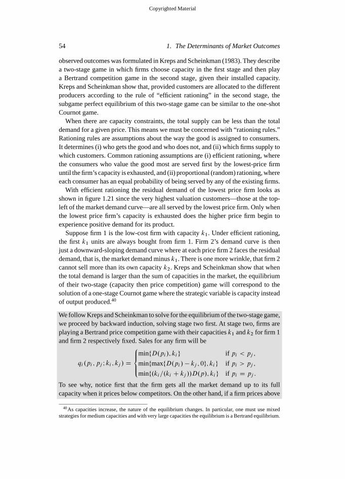
54 1. The Determinants of Market Outcomes
observed outcomes was formulated in Kreps and Scheinkman (1983). They describea two-stage game in which firms choose capacity in the first stage and then playa Bertrand competition game in the second stage, given their installed capacity.Kreps and Scheinkman show that, provided customers are allocated to the differentproducers according to the rule of “efficient rationing” in the second stage, thesubgame perfect equilibrium of this two-stage game can be similar to the one-shotCournot game.
When there are capacity constraints, the total supply can be less than the totaldemand for a given price. This means we must be concerned with “rationing rules.”Rationing rules are assumptions about the way the good is assigned to consumers.It determines (i) who gets the good and who does not, and (ii) which firms supply towhich customers. Common rationing assumptions are (i) efficient rationing, wherethe consumers who value the good most are served first by the lowest-price firmuntil the firm’s capacity is exhausted, and (ii) proportional (random) rationing, whereeach consumer has an equal probability of being served by any of the existing firms.
With efficient rationing the residual demand of the lowest price firm looks asshown in figure 1.21 since the very highest valuation customers—those at the top-left of the market demand curve—are all served by the lowest price firm. Only whenthe lowest price firm’s capacity is exhausted does the higher price firm begin toexperience positive demand for its product.
Suppose firm 1 is the low-cost firm with capacity k1. Under efficient rationing,the first k1 units are always bought from firm 1. Firm 2’s demand curve is thenjust a downward-sloping demand curve where at each price firm 2 faces the residualdemand, that is, the market demand minus k1. There is one more wrinkle, that firm 2cannot sell more than its own capacity k2. Kreps and Scheinkman show that whenthe total demand is larger than the sum of capacities in the market, the equilibriumof their two-stage (capacity then price competition) game will correspond to thesolution of a one-stage Cournot game where the strategic variable is capacity insteadof output produced.40
We follow Kreps and Scheinkman to solve for the equilibrium of the two-stage game,we proceed by backward induction, solving stage two first. At stage two, firms areplaying a Bertrand price competition game with their capacities k1 and k2 for firm 1and firm 2 respectively fixed. Sales for any firm will be
qi .pi ; pj I ki ; kj / D
8<:
minfD.pi /; kig if pi < pj ;
minfmaxfD.pi / � kj ; 0g; kig if pi > pj ;
minf.ki=.ki C kj //D.p/; kig if pi D pj :
To see why, notice first that the firm gets all the market demand up to its fullcapacity when it prices below competitors. On the other hand, if a firm prices above
40As capacities increase, the nature of the equilibrium changes. In particular, one must use mixedstrategies for medium capacities and with very large capacities the equilibrium is a Bertrand equilibrium.
Copyrighted Material

1.3. Competitive Environments 55
its competitor, it will supply any positive residual demand up to its own capacity. Theefficient rationing assumption is thus also embodied in the firm’s assumed demandcurve in the term maxfD.pi /�kj ; 0g. If prices are the same across competitors, weassume that each firm will supply their share of the total capacity available at thatprice.
At the second stage of our game, the firms take capacities as given and choosetheir price to maximize their own profits, for each possible price of rivals. The bestresponse function for each firm at stage 2 is therefore
Ri .pj I ki ; kj / D argmaxpi
�i .pi ; pj I ki ; kj /
D argmaxpi
.pi � c/qi .pi ; pj I ki ; kj /:
There are two possible scenarios. If capacities are large, so large that capacities arenot an effective constraint on sales, then the sales of each firm are
qi .pi ; pj I ki ; kj / D
8<:D.pi / if pi < pj ;
0 if pi > pj ;
.ki=.ki C kj //D.p/ if pi D pj :
In this case, the firm’s demand curve is exactly the one obtained in a Bertrand gamewith homogeneous products, except for the minor difference in the “splitting rule”when prices are equal. As a result, in this case the equilibrium of the subgame willinvolve setting price equal to marginal costs, p� D mc. Since this case is lessinteresting than that of small capacities we focus on that case.
If capacities are small so that capacity constraints are binding, we have
0 6 ki 6 D.pi / � kj 6 D.pi /:
The first inequality follows since capacities are positive. The second illustrates thatcapacity constraints are binding and then capacity is smaller than residual demandat the current price while the latter inequality follows simply since kj is positive.Rearranging the middle inequality gives that total capacity is no larger than demand:
ki C kj 6 D.p/ () ki 6�
ki
ki C kj
�D.p/
and in that case sales will be
qi .pi ; pj I ki ; kj / D
8<:ki if pi < pj ;
minfki ;D.pi / � kj g D ki if pi > pj ;
ki if pi D pj :
Now assuming that equilibrium price adjusts to equate total industry capacity tomarket demand, we have that ki C kj D D.p�/ or, inverting the demand equation,p� D P.ki C kj /.
Copyrighted Material

56 1. The Determinants of Market Outcomes
Market demand curve
Residual demand curve
D( p)
D2 ( p2) qk2k1
D2 ( p2) = D ( p2) − k1
p
Figure 1.21. Residual demand curve with efficient rationing.
If so, then to solve for the equilibrium of the game in stage one, we need tosubstitute the optimal prices p� into the reaction function of the capacity settinggame. That is, each firm solves
Ri .kj / D argmaxki
�i .p�i ; p
�j I ki ; kj /
D argmaxki
.p�i � c/q.p�i ; p
�j I ki ; kj /
D argmaxki
.P.ki C kj / � c/ki :
Clearly, since the objective function is the same as that used in the Cournot model,with qs replaced by ks, the reaction functions derived for the subgame perfectequilibrium of the two-stage game look exactly like the one-shot Cournot gameprofit function with the choice variable being capacity k instead of output q, andwith the inverse demand function P.ki C kj /.
Deneckere and Davidson (1986) show that the Kreps and Scheinkman result issensitive to the exact rationing rule used (see figure 1.21). They argue first thatthe “efficient rationing” is not very likely since under that rule the most highlyvalued units must be bought from the low-price firm. Second, they note that if,for example, consumers are randomly distributed between the two firms, then theKreps and Scheinkman result disappears. On reflection, perhaps the fact that thisresult is sensitive is not really terribly surprising: Kreps and Scheinkman are tryingto ‘compress’ a two-stage game into a simpler and yet equivalent one-stage game—clearly an endeavor which is, at least in general, only going to work under strongand restrictive assumptions.
Copyrighted Material

1.3. Competitive Environments 57
m
k2
KS–Cournot–Nash equilibrium
0 k1k1
mk2
R1 ( k2)
R2 ( k1)
Figure 1.22. Reaction functions in Kreps and Scheinkman two-stage game.
1.3.3 The Monopoly and Dominant-Firm Models
In this section we first briefly revisit the monopoly model and then discuss a vari-ant of that model in which a dominant firm faces a competitive fringe which actsnonstrategically.
1.3.3.1 Monopoly Models
The clearest “dominant” firm model is one in which a firm is a monopoly. Ourbaseline model of such a situation is that a monopolist will simply maximize profitsin a way that is unconstrained by rivals. However, a monopolist may be a price-settingmonopolist, a quantity-setting monopolist, a multiplant quantity-setting monopolistor a multiproduct quantity-setting monopolist or indeed a multiplant, multiproduct,price- or quantity-setting monopolist. Thus there is no single model of a monopoly.In order of complexity static monopoly models of the firm assume that they solveproblems including:
1. Price-setting monopolist: maxp.p � c/D.p/.
2. Quantity-setting monopolist: maxq.P.q/ � c/q.
3. Multiplant, quantity-setting monopolist:
maxq1;:::;qJ
JXjD1
.P.q1 C q2 C � � � C qJ / � cj .qj //qj :
4. Multiproduct, price-setting monopolist:
maxp1;:::;pJ
JXjD1
.pj � cj /Dj .p1; : : : ; pJ /:
Copyrighted Material
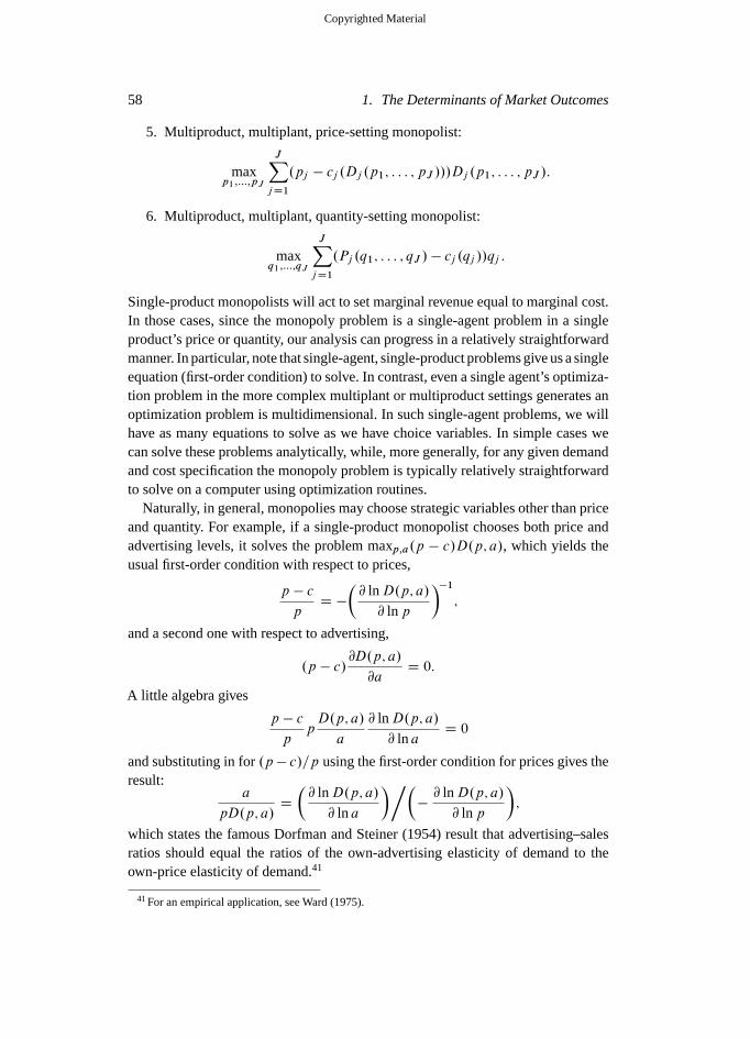
58 1. The Determinants of Market Outcomes
5. Multiproduct, multiplant, price-setting monopolist:
maxp1;:::;pJ
JXjD1
.pj � cj .Dj .p1; : : : ; pJ ///Dj .p1; : : : ; pJ /:
6. Multiproduct, multiplant, quantity-setting monopolist:
maxq1;:::;qJ
JXjD1
.Pj .q1; : : : ; qJ / � cj .qj //qj :
Single-product monopolists will act to set marginal revenue equal to marginal cost.In those cases, since the monopoly problem is a single-agent problem in a singleproduct’s price or quantity, our analysis can progress in a relatively straightforwardmanner. In particular, note that single-agent, single-product problems give us a singleequation (first-order condition) to solve. In contrast, even a single agent’s optimiza-tion problem in the more complex multiplant or multiproduct settings generates anoptimization problem is multidimensional. In such single-agent problems, we willhave as many equations to solve as we have choice variables. In simple cases wecan solve these problems analytically, while, more generally, for any given demandand cost specification the monopoly problem is typically relatively straightforwardto solve on a computer using optimization routines.
Naturally, in general, monopolies may choose strategic variables other than priceand quantity. For example, if a single-product monopolist chooses both price andadvertising levels, it solves the problem maxp;a.p � c/D.p; a/, which yields theusual first-order condition with respect to prices,
p � c
pD �
�@ lnD.p; a/
@ lnp
��1;
and a second one with respect to advertising,
.p � c/@D.p; a/
@aD 0:
A little algebra gives
p � c
ppD.p; a/
a
@ lnD.p; a/
@ ln aD 0
and substituting in for .p � c/=p using the first-order condition for prices gives theresult:
a
pD.p; a/D
�@ lnD.p; a/
@ ln a
����@ lnD.p; a/
@ lnp
�;
which states the famous Dorfman and Steiner (1954) result that advertising–salesratios should equal the ratios of the own-advertising elasticity of demand to theown-price elasticity of demand.41
41 For an empirical application, see Ward (1975).
Copyrighted Material

1.3. Competitive Environments 59
Quantity
Price
Dominant firm marginal revenue
p*
QdominantQfringe
p2
Qtotal
p1
Market demand
Residual demandfacing dominantfirm = D market − S fringe
MC of dominant firm
Supply from fringe
Figure 1.23. Deriving the residual demand curve.
1.3.3.2 The Dominant-Firm Model
The dominant-firm model supposes that there is a monopoly (or collection of firmsacting as a cartel) which is nonetheless constrained to some extent by a competitivefringe. The central assumption of the model is that the fringe acts in a nonstrategicmanner. We follow convention and develop the model within the context of a price-setting, single-product monopoly. Dominant-firm models analogous to each of thecases studied above are similarly easily developed.
If firms which are part of the competitive fringe act as price-takers, they willdecide how much to supply at any given price p. We will denote the supply fromthe fringe at any given price p as S fringe.p/. Because of the supply behavior of thefringe, if they are able to supply whomever they so desire at any given price p, thedominant firm will face the residual demand curve:
Ddominant.p/ D Dmarket.p/ � S fringe.p/:
Figure 1.23 illustrates the market demand, fringe supply, and resulting dominant-firm demand curve. We have drawn the figure under the assumption that (i) thereis a sufficiently high price p1 such that the fringe is willing to supply the wholemarket demand at that price leaving zero residual demand for the dominant firmand (ii) there is analogously a sufficiently low price p2 below which the fringe isentirely unwilling to supply.
Given the dominant firm’s residual demand curve, analysis of the dominant-firmmodel becomes entirely analogous to a monopoly model where the monopolist facesthe residual demand curve, Ddominant.p/. Thus our dominant firm will set prices so
Copyrighted Material

60 1. The Determinants of Market Outcomes
that the quantity supplied will equate the marginal revenue to its marginal cost ofsupply. That level of output is denoted Qdominant in figure 1.23. The resulting pricewill be p� and fringe supply at that price is S fringe.p�/ D Qfringe so that total supply(and total demand) are
Qtotal D Qdominant CQfringe D Sfringe.p�/CDdominant.p�/ D Dmarket.p�/:
A little algebra gives us a useful expression for understanding the role of the fringein this model. Specifically, the dominant firm’s own-price elasticity of demand canbe written as42
�dominantdemand �
@ lnDdominant
@ lnp
D@ ln.Dmarket � S fringe/
@ lnp
D1
Dmarket � S fringe
@.Dmarket � S fringe/
@ lnp
so that we can write
�dominantdemand D
1
Dmarket � S fringe
��Dmarket
Dmarket
�@Dmarket
@ lnp�
�S fringe
S fringe
�@S fringe
@ lnp
�and hence after a little more algebra we have
�dominantdemand D
�Dmarket
Dmarket � S fringe
�@ lnDmarket
@ lnp
�
�S fringe=Dmarket
.Dmarket � S fringe/=Dmarket
�@ ln S fringe
@ lnp
D1
Sharedom �marketdemand �
�Sharefringe
Sharedom
��
fringesupply;
where � indicates a price elasticity. That is, the dominant firm’s demand curve—theresidual demand curve—depends on (i) the market elasticity of demand, (ii) thefringe elasticity of supply, and also (iii) the market shares of the dominant firm andthe fringe. Remembering that demand elasticities are negative and supply elasticitiespositive, this formula suggests intuitively that the dominant firm will therefore facea relatively elastic demand curve when market demand is elastic or when marketdemand is inelastic but the supply elasticity of the competitive fringe is large andthe fringe is of significant size.
42 Recall from your favorite mathematics textbook that for any suitably differentiable function f .x/we can write
@ lnf .x/
@ lnxD
1
f .x/
@f .x/
@ lnx:
Copyrighted Material

1.4. Conclusions 61
1.4 Conclusions
� Empirical analysis is best founded on economic theory. Doing so requiresa good understanding of each of the determinants of market outcomes:the nature of demand, technological determinants of production and costs,regulations, and firm’s objectives.
� Demand functions are important in empirical analysis in antitrust. The elas-ticity of demand will be an important determinant of the profitability of priceincreases and the implication of those price increases for both consumer andtotal welfare.
� The nature of technology in an industry, as embodied in production andcost functions, is a second driver of the structure of markets. For example,economies of scale can drive concentration in an industry while economiesof scope can encourage firms to produce multiple goods within a single firm.Information about the nature of technology in an industry can be retrievedfrom input and output data (via production functions) but also from cost, out-put and input price data (via cost functions) or alternatively data on inputchoices and input prices (via input demand functions.)
� To model competitive interaction, one must make a behavioral assumptionabout firms and an assumption about the nature of equilibrium. Generally, weassume firms wish to maximize their own profits, and we assume Nash equi-librium. The equilibrium assumption resolves the tensions otherwise inherentin a collection of firms each pursuing their own objectives. One must alsochoose the dimension(s) of competition by which we mean defining the vari-ables that firms choose and respond to. Those variables are generally prices orquantity but can also include, for example, quality, advertising, or investmentin research and development.
� The two baseline models used in antitrust are quantity- and price-setting mod-els otherwise known as Cournot and (differentiated product) Bertrand modelsrespectively. Quantity-setting competition is normally used to describe indus-tries where firms choose how much of a homogeneous product to produce.Competition where firms set prices in markets with differentiated or brandedproducts is often modeled using the differentiated product Bertrand model.That said, these two models should not be considered as the only modelsavailable to fit the facts of an investigation; they are not.
� An environment of perfect competition with price-taking firms produces themost efficient outcome both in terms of consumer welfare and productionefficiency. However, such models are typically at best a theoretical abstrac-tion and therefore they should be treated cautiously and certainly should notsystematically be used as a benchmark for the level of competition that canrealistically be implemented in practice.
Copyrighted Material