the determinant of elliptic boundary problems for dirac...
TRANSCRIPT
The Determinant
of Elliptic Boundary Problems
for Dirac Operators –
Reader on
The Scott–Wojciechowski Theorem
Version December 1999
Uncorrected, Incomplete
Compiled, Edited, Revised, Augmented by
B. Booss–Bavnbek
Institut for matematik og fysik, Roskilde University, DK-4000 Roskilde, Denmark
E-mail address : [email protected]

Contents
Part 1. Introductory Material: Determinants of DiracOperators, Spectral Asymmetry, and Grassmannians ofElliptic Boundary Projections 1
Chapter 1. The Idea of the Determinant 31.1. Functional Integrals and Spectral Asymmetry 31.2. The ζ–Determinant for Operators of Infinite Rank 71.3. The Determinant as a Canonical Element of a Complex Line 9
Chapter 2. The ζ–Determinant on the Circle 112.1. ζ– and η–Function of a Dirac operator and the Heat Kernel 122.2. Heat Kernel and ζ–Function on S1 142.3. Duhamel’s Principle and ζ-Function of the Operators ∆f 202.4. Heat Kernel of the Operator D2
a 252.5. η–Invariant - The Phase of the ζ–Determinant 282.6. Modulus of detζDa 34
Chapter 3. The ζ–Determinant on the Interval 373.1. Introduction 373.2. The Variation of the Canonical Determinant 403.3. The Variation of the ζ–Determinant 413.4. The Operator −i d
dx+B(x) - still erronneous 45
Chapter 4. EBVP and Grassmannians 474.1. Dirac Operators - Clifford, Compatible Conn., Product
Structure, Index on Closed Mf., Green’s Formula, CalderonProjector 47
4.2. Global Elliptic Boundary Conditions and Grassmannian(s) 484.3. Boundary Problems defined by Gr∗∞(D): Inverse Operator and
Poisson Maps 50
Chapter 5. Determinant Line Bundles and the Canonical Determinant 575.1. Determinant Bundle 575.2. Canonical Determinant on the Grassmannian Gr∗∞(D) 595.3. Canonical Determinant and Metric 64
Part 2. Spectral Invariants - The Heat Kernel Approach 65
Chapter 6. The Heat Kernel on Gr∞ 676.1. Introduction 67
3
4 CONTENTS
6.2. Duhamel’s Principle and Heat Kernel Estimates 686.3. Duhamel’s Principle 71
Chapter 7. The ζ–Determinant on the Smooth, Self-adjointGrassmannian 79
7.1. Introduction 797.2. Boundary Contribution to the η-Function. I. Unitary Twist
and Duhamel’s Principle 847.3. Boundary Contribution to the η-Function. II. Heat Kernel on
the Cylinder 887.4. The Modulus of the ζ-Determinant on the Grassmannian 937.5. Proof of Theorem 7.3.1 and Proposition 7.4.1 96
Part 3. Pasting of η–Invariants 103
Chapter 8. The Adiabatic Duhamel Principle 1058.1. Introduction 1058.2. Heat Kernels on the Manifold MR
2 1118.3. Dirac Operators on Manifolds with Cylindrical Ends 1208.4. The Estimate of the Lowest Non–Trivial Eigenvalue 1288.5. The Spectrum on the Closed Stretched Manifold 1348.6. The Additivity for Spectral Boundary Conditions 143
Chapter 9. η–Invariant and Variation of the Boundary Condition 1479.1. Variation of η on a Closed Manifold 1479.2. Variation of the Boundary Condition 1509.3. η on the Neck and Additivity Formula 157
Part 4. ζ–Determinant and Fredholm Determinant 161
Chapter 10. The Variation of the Modulus 16310.1. Introduction 16310.2. Variation of the ζ-Determinant on Gr∗∞(D) 169
Chapter 11. Projective equality of the ζ-determinant and Quillendeterminant 175
11.1. Introduction 17511.2. Variation of the Canonical Determinant 18011.3. Equality of the Determinants 185
Chapter 12. Pasting of Determinants 191
Appendix A. The Regularity of the Local η–Function at s = 0 193
Appendix. Bibliography 195
Part 1
Introductory Material: Determinantsof Dirac Operators, Spectral
Asymmetry, and Grassmannians ofElliptic Boundary Projections

CHAPTER 1
The Idea of the Determinant
1
We introduce various notions and problems which will be fun-damental for the book. In particular, we present the basicconcepts of regularization, geometrization, and variation in anon–technical way. First, we recall how Gaussian integralscan be expressed by the determinant. Our model are par-tition functions of classical statistical mechanics involving apositive definit quadratic form on a finite–dimensional space.We discuss various regularization concepts which yield a well–defined finite determinant even when dropping the conditionsof positiveness and of finite dimension, as required by func-tional methods in quantum field theory centred around theDirac operator. We explain the role of the ζ–function in theregularization process and show how the η–invariant naturallyappears which measures the asymmetry of the spectrum andbecomes the phase of the determinant.
Next we explain how the concept of the Fredholm deter-minant can be applied by a geometrization of the underlyingoperator space and without any regularization arbitrariness.
1.1. Functional Integrals and Spectral Asymmetry
Several important quantities in quantum mechanics and quantum fieldtheory are expressed i terms of quadratic functionals and functional inte-grals. The concept of the determinant for Dirac operators arises naturallywhen one wants to evaluate the corresponding path integrals. As Itzyksonand Zuber report in the chapter on Functional Methods of their monograph[55]: “The path integral formalism of Feynman and Kac provides a unifiedview of quantum mechanics, field theory, and statistical models. ... Theoriginal suggestion of an alternative presentation of quantum mechanicalamplitudes in terms of path integrals stems from the work of Dirac (1933)and was brilliantly elaborated by Feynman in the 1940s. ... This work wasfirst regarded with some suspicion due to the difficult mathematics requiredto give it a decent status. In the 1970s it has, however, proved to be the mostflexible tool in suggesting new developments in field theory and thereforedeserves a thorough presentation.”
1Date: November 15, 2001. File name: BOOK1B.TEX, uses BOOKC.STY andBOOKREFE.TEX.
3
4 1. THE IDEA OF THE DETERMINANT
We shall restrict our discussion to the most easy variant of that com-plex matter focusing on the partition function of a quadratic functionalgiven by the Euclidean action of a Dirac operator which is assumed to beelliptic with imaginary time due to Wick rotation and coupled to contin-uously varying vector potentials (sources, fields, connections), for the easeof presentation in vacuum. We refer to Bertlmann, [12] and Schwarz, [90]for an introduction into the quantum theoretic language for mathematiciansand for a more extensive treatment of general aspects of quadratic function-als and functional integrals involving the relations to the Lagrangian andHamiltonian formalism.
There are various alternative notions around, some are more sophisti-cated, some less. In the long run, physics perhaps will show which notionsare the “correct”, the most meaningful ones. At present, mathematics hasalready confirmed the path integral and the ζ–regularized determinant forthe (Euclidean) Dirac operator as notions which lead to reasonable expres-sions, permit precise calculations, and can be understood as canonical ob-jects, independent of particular choices made for regularization. That iswhat we want to show in this book.
A special feature of Dirac operators is that their determinants involvea phase, the imaginary part of the determinant’s logarithm. As we will seenow, this is a consequence of the fact that, unlike the halfbounded Lapla-cian, Dirac operators as operators of first order have an infinite number ofboth positive and negative eigenvalues. Then the phase of the determinantreflects the spectral asymmetry of the corresponding Dirac operator.
The simplest path integral we meet in quantum field theory takes theform of the partition function and can be written formally as the integral
(1.1.1) Z(β) :=
∫Γ
e−βS(ω) dω ,
where dω denotes functional integration over the space Γ := Γ(M ;E) ofsections of a Euclidean vector bundle E over a Riemannian manifold M .
In quantum theoretic language, M is space or space–time; a ω ∈ Γ isa position function of a particle or a spinor field. The scaling parameter βis a real or complex parameter, most often β = 1. The functional S is aquadratic real–valued functional on Γ defined by S(ω) := 〈ω, Tω〉 with afixed linear symmetric operator T : Γ→ Γ. Typically T is a Dirac operatorand S(ω) is the action S(ω) =
∫Mllaω,Dω〉.
Mathematically speaking, the integral 1.1.1 is an oscillating integral likethe Gaussian integral. It is ill–defined in general because
(I) as it stands, it is meaningless when dim Γ(M ;E) = +∞ (i.e., whendimM ≥ 1); and,
(II) even when dim Γ(M ;E) <∞ (i.e. when dimM = 0 and M consistsof a finite set of points), the integral Z(β) diverges unless βS(ω) ispositive and non–degenerate.
1.1. FUNCTIONAL INTEGRALS AND SPECTRAL ASYMMETRY 5
Newertheless, these expressions have been used and construed in quan-tum field theory. As a matter of fact, reconsidering the physicists use andinterpretation of these mathematically ill–defined quantities, one can de-scribe certain formal manipulations which lead to normalizing and evaluat-ing Z(β) in a mathematically rigorous way.
We begin with a few calculations in Case II, inspired by Adams andSen, [1], to show how spectral asymmetry is naturally entering into thecalculations even in the finite–dimensional case and how this suggests thenon–standard definition of the determinant in the infinite–dimensional casefor the Dirac operator.
Then, let dim Γ = d <∞ and set
S(ω) = 〈ω, Tω〉 for all ω ∈ Γ
with a symmetric endomorphism T .
1. calculation. We assume S positive and non–degenerate, i.e. T strictlypositive, T > 0 with specT = {λ1, . . . λd} with all λj > 0. That is theclassical case. We choose an orthonormal system of eigenvectors (e1, . . . , ed)of T as basis for Γ. We have S(ω) =
∑λjx
2j for ω =
∑xjej and get for
real β > 0
Z(β) =
∫Γ
e−βS(ω) dω =
∫Rd
dx1 . . . dxd e−β
∑λjx2
j
=
∫ ∞
−∞e−βλ1x2
1dx1
∫ ∞
−∞e−βλ2x2
2dx2 . . .
∫ ∞
−∞e−βλdx2
ddxd
=
√π
βλ1
√π
βλ2
. . .
√π
βλd
= πd/2 · β−d/2 · (detT )−12 .
In that way the determinant appears when evaluating the simplest quadraticintegral.
2. calculation. If the functional S is positive and degenerate, T ≥ 0, thepartition function is given by
Z(β) = πζ/2 · β−ζ/2 · (det T )−12 · vol(kerT ),
where ζ := dim Γ−dim kerT and T := T |(ker T )⊥ , but, of course vol(kerT ) =∞. For approaches to renormalize this quantity in quantum chromodynam-
ics, we refer to [1], [22], [90]. Still we can take πζ/2β−ζ/2(det T )−12 as our
definition of the integral by discarding vol(kerT ).
3. calculation. Now we assume that the functional S is non–degenerate,i.e. T invertible, but S is neither positive nor negative. We decomposeΓ = Γ+ × Γ− and T = T+ ⊕ T− with T+,−T− strictly positive in Γ±.
6 1. THE IDEA OF THE DETERMINANT
Formally, we obtain
Z(β) =
(∫Γ+
dω+e−β〈ω+,T+ω〉
)(∫Γ−
dω−e−(−β)〈ω−,−T−ω〉
)= πd+/2β−d+/2(detT+)−
12 πd−/2(−β)−d−/2(det−T−)−
12
= πζ/2β−d+/2(−β)−d−/2(det |T |)−12
where d± := dim Γ±, hence ζ = d+ + d− and |T | :=√T 2 = T+ ⊕−T−.
4. calculation. In the preceding formula, the term (β)−d+/2(−β)−d−/2 isundefined for β ∈ R±. We shall replace it by a more intelligible term forβ = 1 by first expanding Z(β) into the upper complex halfplanes and thenformally setting β = 1. More precisely, let β ∈ C+ = {z ∈ C | =z > 0} andwrite β = |β|eiθ with θ ∈ [0, π], hence −β = |β|ei(θ−π) with θ − π ∈ [−π, 0].We set βa := |β|aeiθa and get
β−d+/2(−β)−d−/2 = (|β|eiθ)−d+/2(|β|ei(θ−π))−d−/2
= |β|−ζ/2 e−id+2
θ e−id−2
θ eiπd−2 .
Moreover,
−d+
2θ − d−
2θ + π
d−2
= −θ2
(d+ + d−) +π
2
(d−2
+d+
2+d−2− d+
2
)= −θ
2ζ +
π
4(ζ − η) = −π
4
(2θζ
π+ (η − ζ)
),
where ζ := d+ + d− is the finite–dimensional equivalent of the ζ–invariant ,counting the eigenvalues, and η := d+−d− the finite–dimensional equivalentof the η–invariant , measuring the spectral asymmetry of T . We obtain
Z(β) = πζ/2 |β|−ζ/2e−i π4( 2ζθ
π+(ζ−η)) (det |T |)−
12
and, formally, for β = 1, i.e. θ = 0,
(1.1.2) Z(1) = πζ/2 e−i π4(ζ−η) (det |T |)−
12︸ ︷︷ ︸
=:det T
.
Remark 1.1.1. (a) The methods and results of this section also apply toreal–valued quadratic functionals on complex vector spaces. Since the in-tegration in (1.1.1) in this case is over the real vector space underlyingΓ, which has twice the dimension of Γ, the expressions for the partitionfunctions in this case become the square of those above.(b) In the preceding calculations we worked with ordinary commuting num-bers and functions. The resulting Gaussian integrals are also called bosonicintegrals. If we consider fermionic integrals, we work with Grassmannianvariables and obtain the determinant not in the denominator, but in thenominator (see e.g. [11] or [12]). We shall exploit that aspect later inChapter ???.
1.2. THE ζ–DETERMINANT FOR OPERATORS OF INFINITE RANK 7
(c) Another problem appears even in finite dimensions, namely when adeterminant shall not be defined for a endomorphism but for a homomor-phism.........
Equation (1.1.2) suggests a non–standard definition of the determinantfor the infinite–dimensional case.
1.2. The ζ–Determinant for Operators of Infinite Rank
Once again, our point of departure is finite–dimensional linear algebra.Let T : Cd → Cd be an invertible, positive operator with eigenvalues 0 <λ1 ≤ λ2 ≤ .... ≤ λd . We have the equality
detT =∏
λj = exp{∑
lnλje−s ln λj |s=0}
= exp(− d
ds(∑
λ−sj )|s=0) = e−
dds
ζT (s)|s=0 ,
where ζT (s) :=∑d
j=1 λ−sj .
We show that the preceding formula generalizes naturally, when T isreplaced by a positive definite self–adjoint elliptic operator L (for the easeof presentation, of second order, like the Laplacian) acting on sections of aHermitian vector bundle over a closed manifold M of dimension m. ThenL has a discrete spectrum specL = {λj}j∈N with 0 < λ1 ≤ λ2 ≤ . . . ,satisfying the asymptotic formula λn ∼ nm/2 (see e.g. [45], Lemma 1.6.3).We extend ζL(s) :=
∑∞j=1 λ
−sj in the complex plane by
ζL(s) :=1
Γ(s)
∫ ∞
0
ts−1 Tr e−tL dt
with the Γ–function Γ(s) :=∫∞
0ts−1e−tdt. Note that e−tL is the heat oper-
ator transforming any initial section f0 into a section ft satisfying the heatequation ∂
∂tf + Lf = 0. Clearly Tr e−tL =
∑e−tλj .
One shows that the original definition of ζL(s) yields a holomorphicfunction for <(s) large and that its preceding extension is meromorphic inthe entire complex plane with simple poles only. The point s = 0 is a regularpoint and ζL(s) is a holomorphic function at s = 0. From the asymptoticexpansion of Γ(s) ∼ 1
s+ g + sh(s) close to s = 0 with the Euler number g
and a suitable holomorphic function h we obtain an explicit formula
ζ ′L(0) ∼∫ ∞
0
1
tTr e−tL dt− gζL(0) .
This is proved in xxx / will be proved in xxx.Therefore, Ray and Singer in [84] could introduce detζ(L) by defining:
detζL := e−dds
ζL(s)|s=0 = e−ζ′L(0) .
8 1. THE IDEA OF THE DETERMINANT
The preceding definition does not apply immediately to the main herohere, the Dirac operator D which has infinitely many positive λj and nega-tive eigenvalues −µj. Clearly by the preceding argument
detζD2 = e−ζ′D2 and detζ |D| = e−ζ′|D| = e−
12ζ′D2 .
For the Dirac operator we set
ln detD := − d
dsζD(s)|s=0
with, choosing the branch (−1)−s = eiπs,
ζD(s) =∑
λ−sj +
∑(−1)−sµ−s
j =∑
λ−sj + eiπs
∑µ−s
j
=
∑λ−s
j +∑µ−s
j
2+
∑λ−s
j −∑µ−s
j
2
+ eiπs
{∑λ−s
j +∑µ−s
j
2−∑λ−s
j −∑µ−s
j
2
}=
1
2
{ζD2(
s
2) + ηD(s)
}+
1
2eiπs
{ζD2(
s
2)− ηD(s)
},
where ηD(s) :=∑λ−s
j −∑µ−s
j . Later we will show that ηT (s) is a holo-morphic function of s for <(s) large with a meromorphic extension to thewhole complex plane which is holomorphic in the neighborhood of s = 0 .We obtain
ζ ′D(s) =1
4ζ ′D2(
s
2) +
1
2η′D(s) +
1
2iπeiπs{ζD2(
s
2)− ηD2(s)}
+1
2eiπs{1
2ζ ′D2(
s
2)− η′D(s)}.
It follows:
ζ ′D(0) =1
2ζ ′D2(0) +
iπ
2{ζD2(0)− ηD(0)}
and
detζD = e−12ζ′D2 (0) e−
iπ2 {ζD2 (0)−ηD(0)}
= e−iπ2 {ζ|D|(0)−ηD(0)} e−ζ′|D|(0)
= e−iπ2 {ζ|D|(0)−ηD(0)} detζ |D|,
and for the Dirac operator’s ‘partition function’ in the sense of (1.1.1):
Z(1) = πζ|D|(0)(detζD)−12 .
Remark 1.2.1. In the preceding formulas three spectral invariants enter ofthe Dirac operator D:
1.3. THE DETERMINANT AS A CANONICAL ELEMENT OF A COMPLEX LINE 9
(1) ζD2(0), it is given by∫
Mα(x)dx, where α(x) denotes the index den-
sity which is a certain coefficient in the heat kernel expansion andis locally expressed by the coefficients of D. In particular, ζD2(0)remains unchanged for small changes of the spectrum. Actually,ζL(0) vanishes when L is the square of an self–adjoint elliptic op-erator on a closed manifold.
(2) ηD(0), it is not given by an integral, not by a local formula. Itdepends, however, only on finitely many terms of the symbol ofthe resolvent (D − λ)−1 and will not change when one changes orremoves a finite number of eigenvalues.
(3) ζ ′D2(0), it is the most delicate of the invariants inmvolved: Neitherit is a local invariant, nor does it depend only on the total symbolof the Dirac operator. Below in xxx we will show that even smallchanges of the eigenvalues will change the ζ ′–invariant and hencethe determinant.
Although Felix Klein in [58] rated the determinant as the most simpleexample of an invariant, today we must give an inverse rating. For thepresent authors, not the transformation groups and invariants which revealthe widest symmetries or display the greatest stability are at the centre offocus, but, according to Dirac’s approach to elementary particle physics, thefinest invariants which can detect small anomalies and will be changed outof nearly nothing deserve the highest interest. Correspondingly, the deter-minant and its amplitude (3) are the most subtle and the most fascinatingobjects of our study. They are much more difficult to comprehend than (2);and (2) is much more difficult to comprehend than (1).
For this book, this suggests a scale of stages of investigations. First wehave to show that all three invariants are well defined for Dirac operators onclosed manifolds. Then we shall concentrate on investigating the propertiesof (2), the main ingredient into the determinant’s phase. Then we have toshow that all of them make sense for boundary problems belonging to a cer-tain Grassmannian. Finally, we have to investigate the stability propertiesunder variation of the coefficients.
1.3. The Determinant as a Canonical Element of a Complex Line
Before we do that we discuss another definition of the determinant. Thisone is more algebraic than analytic.
• Fredholm determinant• Segal determinant line• Quillen determinant line• Families

CHAPTER 2
The ζ–Determinant on the Circle
The goal of this chapter is to show how the things works out inthe case of a simple example of the operator Df = −i d
dx +f(x)on the circle S1 . We study the case of the operator Da =−i d
dx + a : C∞(S1)→ C∞(S1) . We show that all ingredientsin the formula (7.4.6) are well-defined and that in fact the ζ-determinant is a true algebraic determinant.
First let us explain why it is enough to study operators Da , when itseems that we should investigate operators of the form
−i ddx
+ f(x) ,
where f(x) denotes a smooth real-valued function on S1 . Let us considertwo such operators
Dfi= −i d
dx+ fi(x) .
and us introduce functions
gi(x) =
∫ x
0
fi(s)ds .
We have now the following result
Proposition 2.0.1. Assume that
(2.0.1) g1(2π) = g2(2π) ,
then operators Df1 and Df2 are unitary equivalent.
Proof. We define operator U acting on functions on S1 via formula
(Us)(x) = ei(g1(x)−g2(x))s(x) .
The operator U is a unitary operator on L2(S1) , and the straightforwardcomputations shows
11
12 2. THE ζ–DETERMINANT ON THE CIRCLE
UDf1U−1 = −i d
dx+ f2(x)
hence Df1 and Df2 are unitary equivalent, which among the other thingsshows that they have the same spectrum. �
Corollary 2.0.2. Operator −i ddx
+ f(x) is unitary equivalent to the oper-
ator −i ddx
+ a , where
(2.0.2) a =
∫ 2π
0f(s)ds
2π.
Corollary 2.0.3. The spectrum of the operator −i ddx
+ f(x) is equal to{k + a}k∈Z , where a is given by the formula (2.0.2).
The last corollary follows from the fact that we know spectrum of theoperator Da = −i d
dx+ a . It has eigenvalues k + a corresponding to the
eigenfunctions φk(x) = 1√2πeikx .
2.1. ζ– and η–Function of a Dirac operator and the Heat Kernel
We study the ζ-determinant of the operator Da using Heat Operatordetermined by D2
a . We start with the discussion of the situation in the caseof a general Dirac operator. Later we prove all results for the operator Da
on S1 . Let D : C∞(M ;S)→ C∞(M ;S) denote a Dirac operator acting onsections of bundle of Clifford modules over a closed manifold M . We wantto solve the Heat Propagation problem for the operator D2 , which meansthat having given f0 ∈ C∞(M ;S) , we want to solve the problem:
(2.1.1) (d
dt+D2)f(t, x) = 0 for t > 0 with f(0, x) = f0(x) .
The problem (2.1.1) has a unique solution for each smooth initial data f0(x)(see for instance [?, ?]). The usual way to get the solution is to construct
a family of operators e−tD2= E(t) : C∞(M ;S) → C∞(M ;S) such that
E(0) = Id and for each f0 and t > 0 we have
(E(t)f0)(x) = f(t, x) .
2.1. ζ– AND η–FUNCTION OF A DIRAC OPERATOR AND THE HEAT KERNEL 13
It is not difficult to see that E(t) staisfies semigroup property i.e. foreach s, t > 0 we have E(t + s) = E(t)E(s) . Moreover operator E(t) has asmooth kernel, which means that there exists a smooth function e(t;x, y) ,where for each x, y ∈M e(t;x, y) is a linear map from Sx to Sy such that
(2.1.2) (e−tD2
f0)(x) = f(t, x) =
∫M
e(t;x, y)f0(y)dy .
Assuming that we know a spectral decomposition of the operator D wehave a nice abstract formula which gives kernel of the Heat Operator. Letus denote by λk an eigenvalue of D , which corresponds to the eigensectionφk . Then we have
(2.1.3) e(t;x, y) =+∞∑−∞
e−tλ2kφk(x)⊗ φk(y) .
In other words we have equality
(E(t)s)(x) =+∞∑−∞
(
∫M
< s(y);φk(y) > dy)φk(x) ,
where < ·; · > denote an inner product on the fibre Sy . We refer to [45] and[?, ?] for more details. In the following we concentrate on a very easy specialcase. Although formula (2.1.3) looks nice it has a relatively small value inthe case we want explicit formula for the kernel e(t;x, y) . We start with thedifferential operator, for which we know exact formula for the kernel andthen study how the perturbation of the operator affects the Heat Kernel.This is what we do in the next Section in order to study ζ-function of theoperator D2
0 = − d2
dx2 on the circle. Now we finally justify the introductionof the Heat Operator. We use this operator in order to study ζ-function andη-function of the Dirac operators.
Proposition 2.1.1. The following equalities hold for a Dirac operator D
(2.1.4) ζD2(s) =1
Γ(s)
∫ ∞
0
ts−1Tr e−tD2
dt for Re(s) >dim M
2,
and
ηD(s) =1
Γ( s+12
)
∫ ∞
0
ts−1Tr De−tD2
dt for Re(s) >1 + dim M
2.
where in the discussion of ζD2(s) we assume that D is invertible. Thisassumption is not necessary in the case of ηD(s) .
14 2. THE ζ–DETERMINANT ON THE CIRCLE
Proof. We prove second equality in (2.1.4). The proof of the first oneis completely analogous. We have
∫ ∞
0
ts−12 Tr De−tD2
dt =+∞∑−∞
∫ ∞
0
ts−12 λke
−tλ2kdt =
+∞∑−∞
λk(λk)−s+12
∫ ∞
0
(tλ2k)
s−12 e−tλ2
kd(tλ2k) =
+∞∑−∞
sign λk·|λk|−s·∫ ∞
0
rs−12 e−rdr = Γ(
s+ 1
2)·ηD(s) .
We discuss the suitable domain of s for which (2.1.4) is valid only for theoperator Df .
�
Remark 2.1.2. If we assume that D has eigenvalue 0 , i.e. there existsnontrivial solution of the equation Ds = 0 , then of course the first formulain (2.1.4) does not hold as the integral on the right side is divergent. To curethis problem we proceed as follows. The operator D is an elliptic operatorhence ker D the space of all solutions of D is finite dimensional and consistsof only smooth sections. This is obvious for the operator Df and we referto [45], or [?, ?] for the proof of this fact for general Dirac operator. Weconsider integral in (2.1.4) on the orthogonal complement of this space, butto stay consistent with the definition (7.1.7) we have to add the dimensionof ker D . More precisely if we denote by ΠD orthogonal projection ontoker D , then first formula in (2.1.4) is replaced by
(2.1.5)
ζD2(s) =1
Γ(s)
∫ ∞
0
ts−1Tr(e−tD2−ΠD)dt+dim ker D for Re(s) >dim M
2.
2.2. Heat Kernel and ζ–Function on S1
We discuss ζ-function of the operator D20 = ∆ = − d2
dx2 on S1 . Weuse formula (2.1.4) hence we need information on the kernel of the operatore−t∆ . It is not difficult to check that eR1(t;x, y) kernel of the correspondingoperator on R1 is given by the formula
eR1(t;x, y) =1√4πt
e−(x−y)2
4t .
Let me repeat again that this means that the function f(t, x) given by theformula
2.2. HEAT KERNEL AND ζ–FUNCTION ON S1 15
f(t, x) = (e−t(− d2
dx2 )f0)(t, x) =
∫R1
1√4πt
e−(x−y)2
4t f0(y)dy
solves the problem (2.1.1) with the initial data f0(x) . Now we define kernelon S1 using the formula
(2.2.1) eS1(t;x, y) =∑n∈Z
eR1(t;x, y + 2πn) .
In (2.2.1) we use the representation of S1 as R/2πZ . Now as the exercisereader may check the following fact
Proposition 2.2.1. The kernel of the operator e−t∆ on S1 is equal toeS1(t;x, y) .
The Proposition 11.3.2 has the following extremely important conse-quence
Theorem 2.2.2. Let us assume that 0 < t < 1 , then there exists positiveconstants c1, c2 , such that the following equality holds
|eS1(t : x, y)− eR1(t;x, y)| < c1·e−c2t .
Remark 2.2.3. (1) The statement of the Theorem 2.2.2 is usually writtenas
(2.2.2) es1(t;x, y) =1√4πt
e−(x−y)2
t +O(e−ct ) for small t .
(2) In the following we really need (7.2.6) for (x, y) close to the diagonalhence the distance between x and y is indeed given by |x− y| .
Proof. We have
es1(t;x, y) =1√4πt
e−(x−y)2
t +1√4πt·∑n6=0
e−(x−y−2πn)2
t ,
16 2. THE ζ–DETERMINANT ON THE CIRCLE
and we estimate sum as follows
∑n6=0
e−(x−y−2πn)2
t =∞∑
k=1
(e−(x−y−2πn)2
t + e−(x−y+2πn)2
t ) < 2·∞∑
k=1
e−(πn)2
4t <
2·∞∑
k=1
(e−π2
4t )n = 2· 1
eπ2
4t
· 1
1− 1
eπ24t
=2
eπ2
4t−1
<2
eπ2
8t
= 2·e−π2
8t .
Now (7.2.6) follows from the elementary estimate
1√t·e−
ct < c1·e−
c2t .
�
Let f, g : (0,∞) → R are smooth functions, then we write f ∼ g ifand only if for any natural number m we have
limt→0
f(t)− g(t)
tm= 0 .
In particular we have just shown that for each x, y ∈ S1
eS1(t;x, y) ∼ 1√4πt
e−(x−y)2
t .
The next Corollary is the first result, which ties spectral geometry westudy with the number theory. It is also at that point that we introducetrace of the heat operator.
Corollary 2.2.4.
(2.2.3)∑n∈N
e−tn2 ∼√π
2·t−1/2 − 1
2.
Proof. We study the trace of the Heat Operator e−t∆ on S1 . Theoperator ∆ has a complete set of eigenvalues with corresponding eigensec-tions given a standard basis of L2(S1) . Namely for any integer k , k2 isan eigenvalue with corresponding eigenfunction φk = 1√
2πeikx . We know
that the trace of the operator can be represented by the eigensections andeigenfunctions as follows (see for instance one of our standard referenceslike [45], and for more of related Functional Analysis [?], or [?, ?]). In ourparticular case we have
2.2. HEAT KERNEL AND ζ–FUNCTION ON S1 17
Tr e−t∆ =∑k∈Z
(e−t∆φk;φk) =∑k∈Z
e−tk2
= 1 + 2·∑n∈N
e−tn2
,
where
(f ; g) =
∫S1
f(x)g(x)dx
is standard L2 product on S1 . On the other hand trace of the operatorwith a smooth kernel is also given by the integral of this kernel over thediagonal
Tr e−t∆ =
∫S1
es1(t;x, x)dx .
Therefore we have
∞∑n=1
e−tn2
=1
2(Tr e−t∆−1) =
1
2(
∫S1
eS1(t;x, x)dx−1) =1
2(
1√4πt
∫S1
dx−1)+O(e−ct ) ,
which finally gives (2.2.3). �
Now we investigate ζ∆(s) ζ-function of the operator. Let us observe thatthis is immediately related to the number theory. Namely if we introduceRiemann ζ-function
ζR(s) =∞∑
n=1
n−s ,
then we have equality
(2.2.4) ζ∆(s) =∑k∈Z
(k2)−s = 2·ζR(2s) + 1 .
This is the reason that we can formulate the main result of this Sectionin terms of the ζR(s) . We have following Theorem
Theorem 2.2.5. Function ζR(s) is a holomorphic function of s for Re(s) >1 . It has a meromorphic extension to complex plane. Point s = 1 is theonly pole of ζR(s) . It is a simple pole and we have
(2.2.5)
Ress=1ζR(s) = 1 , ζR(0) = −1
2and ζR(−2l) = 0 for l = 1, 2, 3, ... .
18 2. THE ζ–DETERMINANT ON THE CIRCLE
Theorem 2.2.5 follows from the corresponding result for the ζ-functionof the operator D0 on S1 . We use representation (2.1.5) . We also need twoproperties of the function Γ(s) . First let us recall that in the neighborhoodof s = 0 , Γ(s) has the following form
(2.2.6) Γ(s) =1
s+ γ + sf(s) =
1 + sγ + s2f(s)
s,
where γ denote Euler constant. We also use the identity
(2.2.7) sΓ(s) = Γ(s+ 1) ,
in order to extend Γ(s) , from the holomorphic function on Re(s) > 1 to ameromorphic function on the whole complex plane. Points sk = −k k =0, 1, 2, .. are the only poles and
(2.2.8) Ress=−kΓ(s) =(−1)k
k!,
as follows from (2.2.6) and (2.2.7). Let us also observe that now we caneasily show that function 1
Γ(s)is a holomorphic function of s on the whole
complex plane and the only zeros of 1Γ(s)
are points sk = −k . Now we are
ready to analyze function ζ∆(s) .
Proposition 2.2.6. Let function h(s) be given by the formula
(2.2.9) h(s) =1
Γ(s)·∫ ∞
1
ts−1Tr(e−tD2 − ΠD)dt .
Then h(s) is a holomorphic function of s on the whole complex plane.
Proof. We estimate Tr(e−tD2 − ΠD) for 1 < t as follows
Tr(e−tD2 − ΠD) = 2∑k∈N
e−tk2
= 2∑k∈N
e−t2k2·e−
t2k2
<
2·e−t2 ·∑k∈N
e−t2k2
< 2·e−t2 ·∑k∈N
e−k2
2 < c·e−t2 ,
and now result follows from elementary complex ananlysis. �
It is integral on the interval 0 < t < 1 , which determines singularitiesof ζ∆(s) . We have
2.2. HEAT KERNEL AND ζ–FUNCTION ON S1 19
1
Γ(s)·∫ 1
0
ts−1Tr(e−tD2−Π(D))dt =1
Γ(s)·∫ 1
0
ts−1(
∫S1
(1√4πt−1+O(e−
ct )dx)dt =
√π
Γ(s)·∫ 1
0
ts−12dt+ g(s) =
√π
Γ(s)· 1
s− 12
− 1
Γ(s)·∫ 1
0
ts−1dt+1
Γ(s)·g(s) ,
where g(s) is yet another function holomorphic on the whole complex planeand we use the fact that
Tr Π(D) = dim ker D = 1 .
We have proved the following Theorem
Theorem 2.2.7. There exists a function g(s) holomorphic on the wholecomplex plane such that ζ∆(s) has the following representation
(2.2.10) ζ∆(s) =
√π
Γ(s)· 1
s− 12
− 1
Γ(s)·1s
+ 1 +1
Γ(s)·g(s) .
We combine this result with
Γ(1
2) =√π and
1
Γ(−k)= 0 for k = 0, 1, 2.. ,
in order to obtain next result
Corollary 2.2.8. The only pole of ζ∆(s) is located at s = 12
. It is a simplepole and the reesiduum of Γ(s) at s = 1 is equal to 1 . Moreover ζ∆(0) = 0and ζ∆(−k) = 1 for k = 1, 2, 3, .. .
Theorem 2.2.5 follows immediately from Corollary 2.2.8 because now wecan use (2.2.10) to represent ζR(s) as
(2.2.11) ζR(s) =1
2(ζ∆(
s
2)− 1) =
√π
Γ( s2)· 1
s− 1− 1
Γ( s2)·1s
+1
2Γ( s2)·g(
s
2) .
20 2. THE ζ–DETERMINANT ON THE CIRCLE
2.3. Duhamel’s Principle and ζ-Function of the Operators ∆f
In this Section we study the ζ-function of the perturbations of the opera-tor ∆ = ∆0 = D2
0 . We discuss in order with increasing technical difficultiesoperators ∆a = ∆ + a , ∆f = ∆ + f(x) , where f(x) is a smooth function
on S1 , and the operator D2a = − d2
dx2 − 2ia ddx
+ a2 . The easiest examplehere is of course operator ∆a . It seems quite natural, that we expect theequality
e−t∆a = e−t∆−ta = e−tae−t∆
to hold, especially becuse the bounded operator (Bf)(x) = af(x) commuteswith the operator ∆ and the equality
e−t(A+B) = e−tAe−tB
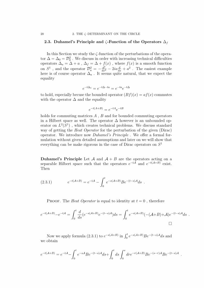
holds for commuting matrices A , B and for bounded commuting operatorsin a Hilbert space as well. The operator ∆ however is an unbounded op-erator on L2(S1) , which creates technical problems. We discuss standardway of getting the Heat Operator for the perturbation of the given (Dirac)operator. We introduce now Duhamel’s Principle . We offer a formal for-mulation without given detailed assumptions and later on we will show thateverything can be make rigorous in the case of Dirac operators on S1
Duhamel’s Principle Let A and A + B are the operators acting on aseparable Hilbert space such that the operators e−tA and e−t(A+B) exist.Then
(2.3.1) e−t(A+B) = e−tA −∫ t
0
e−s(A+B)Be−(t−s)Ads .
Proof. The Heat Operator is equal to identity at t = 0 , therefore
e−t(A+B)−e−tA =
∫ t
0
d
ds(e−s(A+B)e−(t−s)A)ds =
∫ t
0
e−s(A+B)(−(A+B)+A)e−(t−s)Ads .
�
Now we apply formula (2.3.1) to e−s(A+B) in∫ t
0e−s(A+B)Be−(t−s)Ads and
we obtain
e−t(A+B) = e−tA−∫ t
0
e−sABe−(t−s)Ads+
∫ t
0
ds
∫ s
0
dre−r(A+B)Be−(s−r)ABe−(t−s)A .
2.3. DUHAMEL’S PRINCIPLE AND ζ-FUNCTION OF THE OPERATORS ∆f 21
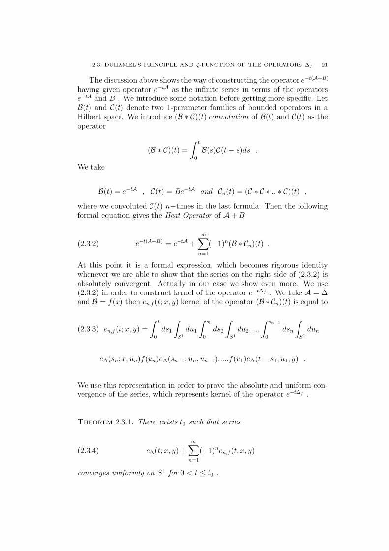
The discussion above shows the way of constructing the operator e−t(A+B)
having given operator e−tA as the infinite series in terms of the operatorse−tA and B . We introduce some notation before getting more specific. LetB(t) and C(t) denote two 1-parameter families of bounded operators in aHilbert space. We introduce (B ∗ C)(t) convolution of B(t) and C(t) as theoperator
(B ∗ C)(t) =
∫ t
0
B(s)C(t− s)ds .
We take
B(t) = e−tA , C(t) = Be−tA and Cn(t) = (C ∗ C ∗ .. ∗ C)(t) ,
where we convoluted C(t) n−times in the last formula. Then the followingformal equation gives the Heat Operator of A+B
(2.3.2) e−t(A+B) = e−tA +∞∑
n=1
(−1)n(B ∗ Cn)(t) .
At this point it is a formal expression, which becomes rigorous identitywhenever we are able to show that the series on the right side of (2.3.2) isabsolutely convergent. Actually in our case we show even more. We use(2.3.2) in order to construct kernel of the operator e−t∆f . We take A = ∆and B = f(x) then en,f (t;x, y) kernel of the operator (B ∗ Cn)(t) is equal to
(2.3.3) en,f (t;x, y) =
∫ t
0
ds1
∫S1
du1
∫ s1
0
ds2
∫S1
du2.....
∫ sn−1
0
dsn
∫S1
dun
e∆(sn;x, un)f(un)e∆(sn−1;un, un−1).....f(u1)e∆(t− s1;u1, y) .
We use this representation in order to prove the absolute and uniform con-vergence of the series, which represents kernel of the operator e−t∆f .
Theorem 2.3.1. There exists t0 such that series
(2.3.4) e∆(t;x, y) +∞∑
n=1
(−1)nen,f (t;x, y)
converges uniformly on S1 for 0 < t ≤ t0 .
22 2. THE ζ–DETERMINANT ON THE CIRCLE
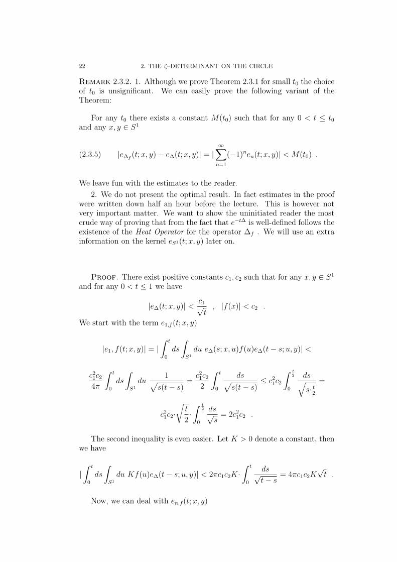
Remark 2.3.2. 1. Although we prove Theorem 2.3.1 for small t0 the choiceof t0 is unsignificant. We can easily prove the following variant of theTheorem:
For any t0 there exists a constant M(t0) such that for any 0 < t ≤ t0and any x, y ∈ S1
(2.3.5) |e∆f(t;x, y)− e∆(t;x, y)| = |
∞∑n=1
(−1)nen(t;x, y)| < M(t0) .
We leave fun with the estimates to the reader.
2. We do not present the optimal result. In fact estimates in the proofwere written down half an hour before the lecture. This is however notvery important matter. We want to show the uninitiated reader the mostcrude way of proving that from the fact that e−t∆ is well-defined follows theexistence of the Heat Operator for the operator ∆f . We will use an extrainformation on the kernel eS1(t;x, y) later on.
Proof. There exist positive constants c1, c2 such that for any x, y ∈ S1
and for any 0 < t ≤ 1 we have
|e∆(t;x, y)| < c1√t, |f(x)| < c2 .
We start with the term e1,f (t;x, y)
|e1, f(t;x, y)| = |∫ t
0
ds
∫S1
du e∆(s;x, u)f(u)e∆(t− s;u, y)| <
c21c24π
∫ t
0
ds
∫S1
du1√
s(t− s)=c21c2
2
∫ t
0
ds√s(t− s)
≤ c21c2
∫ t2
0
ds√s· t
2
=
c21c2·√t
2·∫ t
2
0
ds√s
= 2c21c2 .
The second inequality is even easier. Let K > 0 denote a constant, thenwe have
|∫ t
0
ds
∫S1
du Kf(u)e∆(t− s;u, y)| < 2πc1c2K·∫ t
0
ds√t− s
= 4πc1c2K√t .
Now, we can deal with en,f (t;x, y)
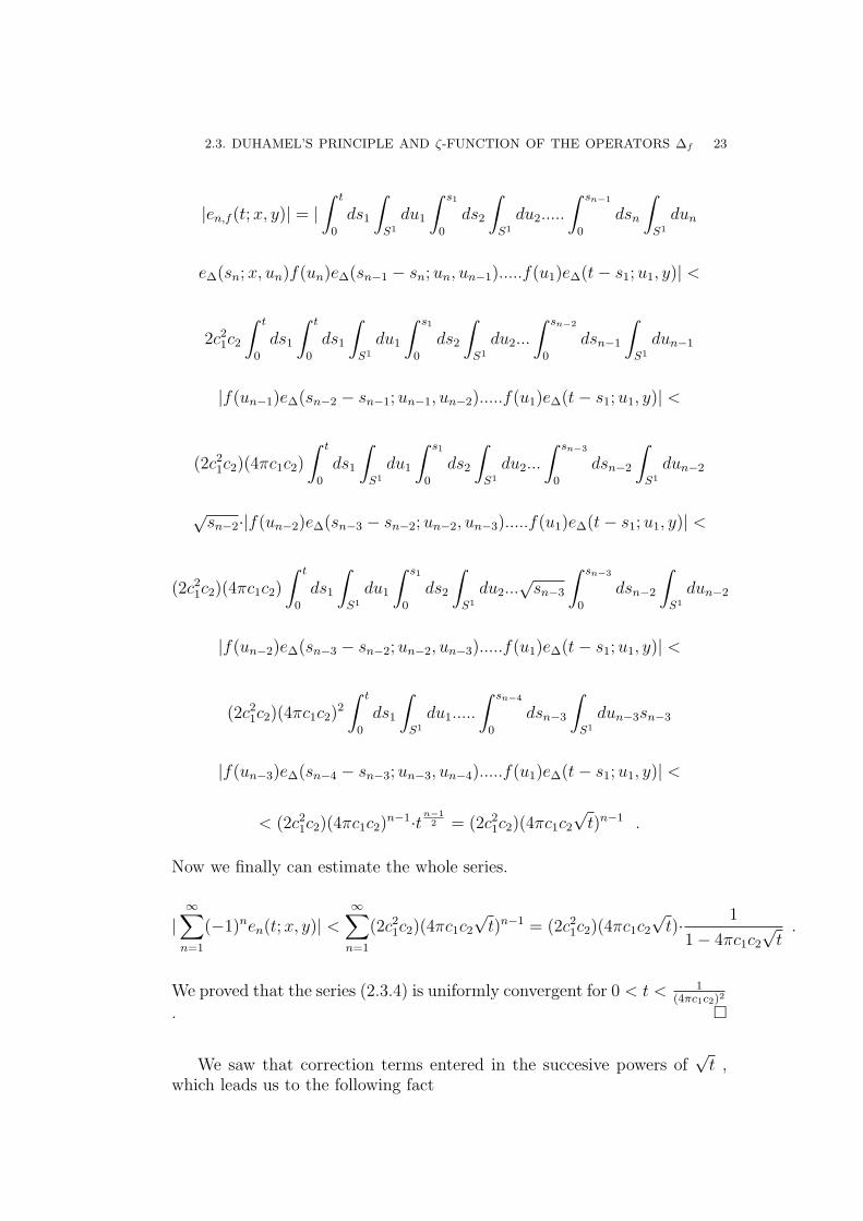
2.3. DUHAMEL’S PRINCIPLE AND ζ-FUNCTION OF THE OPERATORS ∆f 23
|en,f (t;x, y)| = |∫ t
0
ds1
∫S1
du1
∫ s1
0
ds2
∫S1
du2.....
∫ sn−1
0
dsn
∫S1
dun
e∆(sn;x, un)f(un)e∆(sn−1 − sn;un, un−1).....f(u1)e∆(t− s1;u1, y)| <
2c21c2
∫ t
0
ds1
∫ t
0
ds1
∫S1
du1
∫ s1
0
ds2
∫S1
du2...
∫ sn−2
0
dsn−1
∫S1
dun−1
|f(un−1)e∆(sn−2 − sn−1;un−1, un−2).....f(u1)e∆(t− s1;u1, y)| <
(2c21c2)(4πc1c2)
∫ t
0
ds1
∫S1
du1
∫ s1
0
ds2
∫S1
du2...
∫ sn−3
0
dsn−2
∫S1
dun−2
√sn−2·|f(un−2)e∆(sn−3 − sn−2;un−2, un−3).....f(u1)e∆(t− s1;u1, y)| <
(2c21c2)(4πc1c2)
∫ t
0
ds1
∫S1
du1
∫ s1
0
ds2
∫S1
du2...√sn−3
∫ sn−3
0
dsn−2
∫S1
dun−2
|f(un−2)e∆(sn−3 − sn−2;un−2, un−3).....f(u1)e∆(t− s1;u1, y)| <
(2c21c2)(4πc1c2)2
∫ t
0
ds1
∫S1
du1.....
∫ sn−4
0
dsn−3
∫S1
dun−3sn−3
|f(un−3)e∆(sn−4 − sn−3;un−3, un−4).....f(u1)e∆(t− s1;u1, y)| <
< (2c21c2)(4πc1c2)n−1·t
n−12 = (2c21c2)(4πc1c2
√t)n−1 .
Now we finally can estimate the whole series.
|∞∑
n=1
(−1)nen(t;x, y)| <∞∑
n=1
(2c21c2)(4πc1c2√t)n−1 = (2c21c2)(4πc1c2
√t)· 1
1− 4πc1c2√t.
We proved that the series (2.3.4) is uniformly convergent for 0 < t < 1(4πc1c2)2
. �
We saw that correction terms entered in the succesive powers of√t ,
which leads us to the following fact
24 2. THE ζ–DETERMINANT ON THE CIRCLE
Corollary 2.3.3. There exists a family {un(x)}n∈N of smooth functionson S1 such that for any natural number N we have
(2.3.6) e∆f(t;x, x)−
N∑n=0
tn−1
2 un(x) = O(tN) .
The last result is not really the best we can get. We know (see forinstance [45, ?]) that actually we have expansion in powers of t . This resultis acxtually quite difficult to establish in the case of a general Dirac operator.In the case of S1 we can use the fact that, for any 0 < t and any x, y ∈ S1
e∆(t;x, y) > 0 (see (2.2.1). We also use the fact that identity e−s∆e−(t−s)∆ =e−t∆ reads as follows on the level of the kernel of the operators
(2.3.7)
∫S1
e∆(s;x, u)e∆(t− s;u, y)du = e∆(t;x, y) .
Theorem 2.3.4. There exists a family {vn(x)}n∈N of smooth functions onS1 such that for any natural number N we have
(2.3.8) e∆f(t;x, x)−
N∑n=0
tn−12vn(x) = O(tN) .
Proof. As I promised we show that indeed correction terms enter inpowers of t . Let us explain that on the level of the first term
|∫ t
0
ds
∫S1
du e∆(s;x, u)f(u)e∆(t−s;u, y)| < c2·∫ t
0
ds
∫S1
du e∆(s;x, u)e∆(t−s;u, y) =
c2·∫ t
0
e∆(t;x, y)ds = c2t·e∆(t;x, y) .
The estimate on the n − th term of the expansion follows in the sameway. �
Corollary 2.3.5. For any f(x) smooth function on S1 we have
ζ∆f(0) = 0 .
2.4. HEAT KERNEL OF THE OPERATOR D2a 25
Proof. The result follows from the corresponding result for ∆ as wehave just proved that there exists a positive constant c such that the fol-lowing estimate holds
|e∆f(t;x, y)− e∆(t;x, y)| < c
√t ,
for any x, y ∈ S1 and any 0 < t ≤ 1 . Let Π∆fdenote orthogonal projection
onto the kernel of the operator ∆f . Then we have
ζ∆f(s) =
1
Γ(s)
∫ ∞
0
ts−1Tr(e−t∆f − Π∆f)dt+ dim ker ∆f =
1
Γ(s)
∫ 1
0
ts−1Tr(e−t∆f − Π∆f)dt+ dim ker ∆f +
1
Γ(s)·h(s) ,
where h(s) is a function holomorphic on the whole complex plane. Trace ofΠ∆f
is equal to dim ker ∆f and therefore we have
ζ∆f(s) =
1
Γ(s)
∫ 1
0
ts−1Tr e−t∆fdt+(dim ker ∆f )·(1− 1
Γ(s)
∫ 1
0
ts−1ds)+1
Γ(s)·h(s) =
1
Γ(s)
∫ 1
0
ts−1(
√π√t
+O(√t))dt+ (dim ker ∆f )·(1− s
Γ(s)) +
1
Γ(s)·h(s) =
√π
Γ(s)· 1
s− 12
+1
Γ(s)
∫ 1
0
ts−1O(√t)dt+(dim ker ∆f )·(1− s
Γ(s))+
1
Γ(s)·h(s) .
We take lims→0 and obtain 0 .�
As the exercise reader may use Duhamel’s Principle to check that
(2.3.9) e∆+a(t;x, y) = e−tae∆(t;x, y) .
2.4. Heat Kernel of the Operator D2a
In this Section we use Duhamel’s Principle to construct kernel of theoperator e−tD2
a on S1 . Our goal is to prove analogue of Theorem 2.3.4 inthis new situation. We have
D2a = −∆− 2ia
d
dx+ a2 = −∆ + 2aD0 + a2 .
We know that we do not have any problem with a2 . We simply have:
26 2. THE ζ–DETERMINANT ON THE CIRCLE
e−∆+2aD0+a2(t;x, y) = e−ta2
e−∆+2aD0(t;x, y) .
The problem here is that the perturbation is now of order 1 , hence it is nota bounded operator on L2(S1) . Stil we can study kernel of the operatore−∆+2aD0 the way we did it in a previous Section. We have to show absoluteconvergence of the series
(2.4.1) e∆(t;x, y) +∞∑
n=1
en,Da(t;x, y) ,
where
en,Da(t;x, y) =
∫ t
0
ds1
∫S1
du1
∫ s1
0
ds2
∫S1
du2.....
∫ sn−1
0
dsn
∫S1
dun
e∆(sn;x, un)2aD0e∆(sn−1;un, un−1).....2aD0e∆(t− s1;u1, y) .
Let us first figure out the straightforward estimates on en,Da(t;x, y) . Wehave
|e1,Da(t;x, y)| = 2a·|∫ t
0
ds
∫S1
e∆(s;x, u)(d
du)e∆(t− s;u, y)| ≤
2a1
4π·∫ t
0
ds√s(t− s)
∫S1
e−(x−u)2
4t · |u− y|2(t− s)
e−(u−y)2
4t ≤
2a1
4π·∫ t
0
ds√s(t− s)
∫S1
|u− y|2(t− s)
e−(u−y)2
4t <2
4π·∫ t
0
ds√s(t− s)
∫ ∞
0
z
2(t− s)e−
z2
4t =
2a1
2π
∫ t
0
ds√s(t− s
≤ 2a1
2π
2
t·∫ t
0
ds = 2a1
π.
More general we have
(2.4.2) |en,Da(t;x, y)| < 1
π(2a)n 1
12·32·...·n−1
2
(1√π
)n−1tn−1
2 ,
and as in Section 2.3 we proved the uniform and absolute convergence of theseries which formally gives kernel of the operator e−∆+2aD0 , hence we havejust constructed this kernel. Actually again we expect that terms with oddn should disappear. This follows from the general theory (see for instance[45] Chapter 1, or [?]). However in our case we can offer a simple argument
which shows that Tr e−tD2a expands in powers of t rather than
√t .
2.4. HEAT KERNEL OF THE OPERATOR D2a 27
Theorem 2.4.1. There exists a sequence of real numbers {rk}∞k=0 such thatfor any natural number N we have
(2.4.3) Tr e−tD2a −
N∑k=0
tk−12 rk = O(tN) .
Remark 2.4.2. If we work harder we would be able to prove that thereexist a sequence of smooth functions {fk(x)} such that
eD2a(t;x, x)−
N∑k=0
tk−12fk(x) = O(tN) .
This “Local Variant” of Theorem 2.4.1 for the general Dirac operator isproved in [45, ?] .
Proof. We use the fact that operators ∆ and D0 = −i ddx
commute.
Now we write a series which gives the operator e−t(∆+2aD0)
e−t(∆+2aD0) = e−t∆ + (−1)nEn(t) ,
where
En(t) = (2a)n
∫ t
0
ds1
∫ s1
0
ds2...
∫ sn−1
0
dsne−sn∆D0e
−(sn−1−sn)∆D0...D0e−(t−s1)∆ =
(2a)n(D0)ne−t∆·
∫ t
0
ds1
∫ s1
0
ds2...
∫ sn−1
0
dsn = (2a)n· tn
n!(D0)
ne−t∆ .
Now Theorem 2.4.1 follows from the fact that D0 = −i ddx
has symmetricspectrum which implies the equality
Tr D2n+10 e−tD2
= 0 ,
for any natural number n .�
Corollary 2.4.3. For any real a
(2.4.4) ζD2a(0) = 0 .
28 2. THE ζ–DETERMINANT ON THE CIRCLE
Proof. The result follows from the fact that we have just proved
Tr e−tD2a − Tr e−tD2
0 <c√t,
for 0 < t < 1 . �
2.5. η–Invariant - The Phase of the ζ–Determinant
In this Section we study the η-invariant of the operator Da . The mainresult is
Theorem 2.5.1. The function ηDa(s) is a holomorphic function of s forRe(s) > −2 .
Once again we prove this result by studying Heat Kernels. We rememberformula
ηDa(s) =1
Γ( s+12
)·∫ ∞
0
ts−12 Tr Dae
−tD2adt .
We now decompose Tr Dae−tD2
a and use the fact that Tr D0e−tD2
0 is equalto 0
Tr Dae−tD2
a = Tr Dae−tD2
a − Tr D0e−tD2
0 =
Tr(Da−D0)e−tD2
a−Tr D0(e−tD2
a−e−tD20) = a·Tr e−tD2
a−Tr D0(e−tD2
a−e−tD20) .
We know the expansion of the first summand on the right side
(2.5.1) a·Tr e−tD2a − a·
√π
t+ c1·
√t = O(t
32 ) .
Now we remember that
e−tD2a = e−ta2
e−t(∆−2aD0) = e−ta2
(e−t(∆−2aD0) − e−t∆) + e−ta2
e−t∆ ,
and we have to study now
(2.5.2)
Tr D0(e−tD2
a−e−tD20) = Tr e−ta2D0(e
−t(∆−2aD0)−e−t∆)+Tr (e−ta2−Id)D0e−t∆ .
2.5. η–INVARIANT - THE PHASE OF THE ζ–DETERMINANT 29
The second term on the right side is again equal to 0 and finally we onlyhave to show that Tr e−ta2D0(e
−t(∆−2aD0)−e−t∆) has the correct asymptotic.It was already observed in Section 2.4 that
(2.5.3) e−t(∆−2aD0) − e−t∆ =∞∑
n=1
(2at)n
n!Dn
0 e−t∆ .
hence we do have
Tr D0(e−tD2
a − e−tD20) = Tr e−ta2D0e
−t(∆−2aD0) =
Tr e−ta2∞∑
n=1
(2at)n
n!Dn+1
0 e−t∆ = Tr e−ta2∞∑
k=1
(2at)2k−1
(2k − 1)!D2k
0 e−t∆ .
Now let us use an extra symmetry we have in this formula
(2.5.4) Tr D2k0 e
−t∆ = (−1)k(d
dt)k(Tr e−tD2
) = (−1)k(d
dt)k(
√π√t
+O(e−ct )) .
We have proved following result
Proposition 2.5.2. There exist a sequence of constants {bk} such that
(2.5.5) Tr Dae−tD2
a ∼ b0√t
+ b1√t+ ... .
However we are not out of trouble if the situation in the neighborhoodof s = 0 is concerned. This is due to the fact that we have to study
lims→0
1
Γ( s+12
)
∫ ∞
0
ts−12 Tr Ddae
−tD2adt ,
and in this situation factor 1Γ(s)
is replaced by 1Γ( s+1
2)
, hence the singularity
which comes from the heat kernel is not cancelled by singularity of Γ(s) .Now, when you study more precisely formulas (2.5.1) and (7.2.3) . We cometo a conclusion that actually we have
(2.5.6) b0 = 0 ,
30 2. THE ζ–DETERMINANT ON THE CIRCLE
in (2.5.5), but as in these notes a focus is on different methods related toHeat Kernel we offer yet another argument. This type of argument is usedquite often in different contexts in Spectral Geometry. We define a function
R(a) = Ress=0ηDa(0) .
Theorem 2.5.3.
(2.5.7)dRda
= 0
We need the next Lemma in the proof of Theorem 2.5.3.
Lemma 2.5.4.
(2.5.8) ˙e−tD2a =
d
da(e−tD2
a) = −∫ t
0
e−sD2a(DaDa +DaDa)e−(t−s)D2
ads .
Remark 2.5.5. Of course (2.5.8) is the formula which holds for the smooth,1-parameter family of Dirac operators over closed manifold. In the partic-ular case of the operator Da = −i d
dx+ a on S1 , we have Da = dDa
da= 1 and
(2.5.8) becomes
˙e−tD2a = −2
∫ t
0
Dae−tD2
ads = −2tDae−tD2
a .
Proof. In the Lemma 2.5.4 we study variation of the Heat Kernel underthe smooth change of the Dirac operator
d
da{e−tD2
a} = limr→0
1
r·(e−tD2
a+r − e−tD2a) = lim
r→0
1
r·∫ t
0
d
ds(e−sD2
a+re−(t−s)D2a)ds =
limr→0
1
r·∫ t
0
e−sD2a+r(D2
a −D2a+r)e
−(t−s)D2ads =
limr→0
∫ t
0
e−sD2aD2
a −D2a+r
re−(t−s)D2
ads+limr→0
∫ t
0
1
r(e−sD2
a+r−e−sD2a)(D2
a−D2a+r)e
−(t−s)D2ads =
2.5. η–INVARIANT - THE PHASE OF THE ζ–DETERMINANT 31
−∫ t
0
e−sD2aD2
ae−(t−s)D2
ads+ 0 = −∫ t
0
e−sD2a(DaDa +DaDa)e−(t−s)D2
ads .
�
Proof. Now we are ready to prove Theorem 2.5.3.
We have
(2.5.9) R(a) = lims→0
s· 1
Γ( s+12
)
∫ ∞
0
ts−12 Tr Dae
−tD2adt .
and we study the variation of the integral on the right side of (2.5.9).
d
da{∫ ∞
0
ts−12 Tr Dae
−tD2adt} =
∫ ∞
0
ts−12 Tr Dae
−tD2adt+
∫ ∞
0
ts−12 Tr Da{ ˙e−tD2
a}dt =
∫ ∞
0
ts−12 Tr Dae
−tD2adt+
∫ ∞
0
ts−12 Tr Da
˙e−tD2adt =
∫ ∞
0
ts−12 Tr Dae
−tD2adt−2
∫ ∞
0
ts−12 Tr tDaD2
ae−tD2
a =
∫ ∞
0
ts−12 Tr Dae
−tD2adt+
2
∫ ∞
0
ts+12d
dt(Tr Dae
−tD2a)dt =
∫ ∞
0
ts−12 Tr Dae
−tD2adt+2 lim
ε→0(t
s+12 Tr Dae
−εD2a)|
1εε−
2
∫ ∞
0
d
dt(t
s+12 )Tr Dae
−tD2adt .
The limit
limε→0
(ts+12 Tr Dae
−εD2a)|
1εε
is equal to 0 for the invertible operator Da and s > 0 and we obtain a crucialformula
(2.5.10)d
da{∫ ∞
0
ts−12 Tr Dae
−tD2adt} = −s
∫ ∞
0
ts−12 Tr Dae
−tD2adt .
Once again formula simplifies in the case of Da on S1 as Da = 1 . Now wefinally have information about the variation of the residuum
dRda
=d
dalims→0
s·ηDa(s) = − lims→0
s
Γ( s+12
)
d
da{∫ ∞
0
ts−12 Tr Dae
−tD2adt} =
32 2. THE ζ–DETERMINANT ON THE CIRCLE
− 1√π
lims→0
s2
∫ ∞
0
ts−12 Tr e−tD2
adt = 0
�
Let us observe that in fact we also obtain the formula for the variationof the η-invariant i.e. the number ηDa(0) .
ηDa(0) = lims→0
−sΓ( s+1
2)
∫ ∞
0
ts−12 Tr e−tD2
adt = − 1√π· lim
s→0s·∫ 1
0
ts−12 Tr e−tD2
adt =
− 1√π· lim
s→0s·∫ 1
0
ts−12 (
√π
t+r1√t+O(t
32 ))dt = − 1√
π· lim
s→0s·∫ 1
0
ts−12
√π
tdt =
− lims→0
s·∫ 1
0
ts2−1dt = − lim
s→0s·1s
2
= −2 .
Theorem 2.5.3 implies that ηDa(s) is a holomorphic function of s in theneighborhood of s = 0 , beacause we know that
R(0) = 0 ,
and by Theorem 2.5.3 , this extends to any real number a . In fact we haveproved more, because equality (2.5.5) implies that there exists constantc > 0 such that for any 0 < t ≤ 1 we have
(2.5.11) |Tr Dae−tD2
a| < c√t ,
which gives us representation
Tr Ddae−tD2
a = b1√t+ b2t
32 +O(t
52 ) .
Now we can discussed structure of the η-function of Da
1
Γ( s+12
)
∫ ∞
0
ts−12 Tr De−tD2
adt =1
Γ( s+12
)
∫ ∞
0
ts−12 (b1
√t+ b2t
32 +O(t
52 ))dt =
1
Γ( s+12
)
∫ 1
0
ts−12 (b1
√t+ b2t
32 +O(t
52 ))dt+ h(s) =
b1Γ( s+1
2)
∫ 1
0
ts2dt+
b2Γ( s+1
2)
∫ 1
0
ts2+1 + h1(s) + h(s) ,
where h(s) is a holomorphic function on the whole complex plane and h1(s)is holomorphic for Re(s) > −6 . This shows that there exists h2(s) afunction holomorphic for Re(s) > −6 , such that
2.5. η–INVARIANT - THE PHASE OF THE ζ–DETERMINANT 33
(2.5.12) ηDa(s) =b1
Γ( s+12
)· 2
s+ 2+
b2Γ( s+1
2)· 2
s+ 4+ h2(s) .
In particular Theorem 2.5.1 is proved.
Corollary 2.5.6.
(2.5.13) ηDa(0) =1√π
∫ ∞
0
1√tT r Dae
−tD2adt .
Proof. Theorem 2.5.1 implies that we can apply second formula in(2.1.4) for any s with Re(s) > −2 . �
Corollary 2.5.7.
(2.5.14) ηDa(0) = − 2√π· lim
ε→0
√ε·Tr Dae
−εD2a ,
which in the case of operator Da on S1 gives ηDa(0) = −2 .
Proof. We differentiate equation (2.5.14)
d
daηDa(0) =
d
da(
1√π
∫ ∞
0
1√tT r Dae
−tD2adt) =
1√π
∫ ∞
0
1√tT r Dae
−tD2adt+
2√π
∫ ∞
0
√t· ddt
(Tr Dae−tD2
a)dt =1√π
∫ ∞
0
1√tT r Dae
−tD2adt+
2√π· lim
ε→0(√t·Tr Dae
−tD2a)|
1εε−
1√π
∫ ∞
0
1√tT r Dae
−tD2adt = − 2√
π· lim
ε→0
√ε·Tr Dae
−εD2a .
In the case of Da on S1 we have
− 2√π· lim
ε→0
√ε·Tr Dae
−εD2a = − 2√
π· lim
ε→0
√ε·(√π
ε+O(
√ε)) = −2 .
�
34 2. THE ζ–DETERMINANT ON THE CIRCLE
Theorem 2.5.8.
(2.5.15) ηDa(0) = 1− 2a .
Proof. We have just proved that
ηDa(0) = −2a mod Z .
More precisely ηDa(0) continous part of ηDa(0) (as function of a) is equal to−2a . Now we see that we can argue that formula
ηDa(s) =1
as+∑k 6=0
sign(k + a)|k + a|s
invites us to put lims→0 ηDa(s) = 1 + ηDa(0) = 1 − 2a . However, we canargue for some other choice as well. As we can see in the next section ourchoice of the integer comes from the determinant theory. �
It follows now from Theorem 2.5.8 and Corollary 2.4.3 that we know thephase of the ζ-determinant of the operator Da
Corollary 2.5.9. The pahse of the detζDa is eqqual to e2a−1 .
In the next Section we deal with the modulus of the ζ-determinant.
2.6. Modulus of detζDa
There are some reason beyond the scope of this notes (see for instance[94, 95], which tell us that we should pick up the operator D 1
2= −i d
dx+ 1
2
and assume that its ζ-determinant is equal to 1 and then obtain the valueof the ζ-determinant for other Da by studying variation of the determinantwith respect to a. We will show later on that we also obtain equality
detζD 12
= 1
from the argument from Elementary Number Theory. We start howeverwith study of the variation of the modulus with respect to the parametera . Now, then phase is − half of ζ ′D2
a(0) = d
dsz′D2
a(s)|s=0 . We know that
ζD2a(s) is holomorphic in the neighborhood of s = 0 and we can take the
derivative with respect to s , which gives
2.6. MODULUS OF detζDa 35
lims→0
d
ds(
1
Γ(s)
∫ ∞
0
ts−1Tr e−tD2adt) = lim
s→0(−Γ′(s)
Γ(s)2
∫ ∞
0
ts−1Tr e−tD2adt)+
lims→0
(1
Γ(s)
d
ds(
∫ ∞
0
ts−1Tr e−tD2adt)) = lim
s→0(−Γ′(s)
Γ(s)2
∫ ∞
0
ts−1Tr e−tD2adt) .
Remark 2.6.1. The fact that lims→0(1
Γ(s)dds
(∫∞
0ts−1Tr e−tD2
adt)) dissapear
is due to the absence of the singularity of the functionK(s) =∫∞
0ts−1Tr e−tD2
adtat s = 0 and it is characteristic for dimension 1 , or more general for odd di-mensional manifold M . In the even-dimensional case this part may produceadditonal contribution.
We know that Γ′(s) = − 1s2 +h(s) , where h(s) is a holomorphic function
in the neighborhood of s = 0 , hence we arrived at the equation
(2.6.1)d
ds(
1
Γ(s)
∫ ∞
0
ts−1Tr e−tD2adt)|s=0 = lim
s→0
∫ ∞
0
ts−1Tr e−tD2adt =
∫ ∞
0
1
t·Tr e−tD2
adt .
We use Lemma 2.5.4 to study the variation of the right side of (2.6.1)and obtain
(2.6.2)d
da
∫ ∞
0
1
t·Tr e−tD2
adt = −2·∫ ∞
0
Tr DaDae−tD2
adt = −2·∫ ∞
0
Tr Dae−tD2
adt = −2·ηDa(1) .
We work on the expression∫∞
0Tr Dae
−tD2adt in order to obtain the
variation. We may assume that Da is invertible, hence∫ ∞
0
Tr Dae−tD2
adt =
∫ ∞
0
Tr D−1a D2
ae−tD2
adt = −∫ ∞
0
d
dt(Tr D−1
a e−tD2a)dt =
limε→0
(Tr D−1a e−tD2
a)|1εε = − lim
ε→0Tr D−1
a e−εD2a .
We have just proved
Proposition 2.6.2.
(2.6.3)d
daζ ′D2
a(0) = 2· lim
ε→0Tr D−1
a e−εD2a .
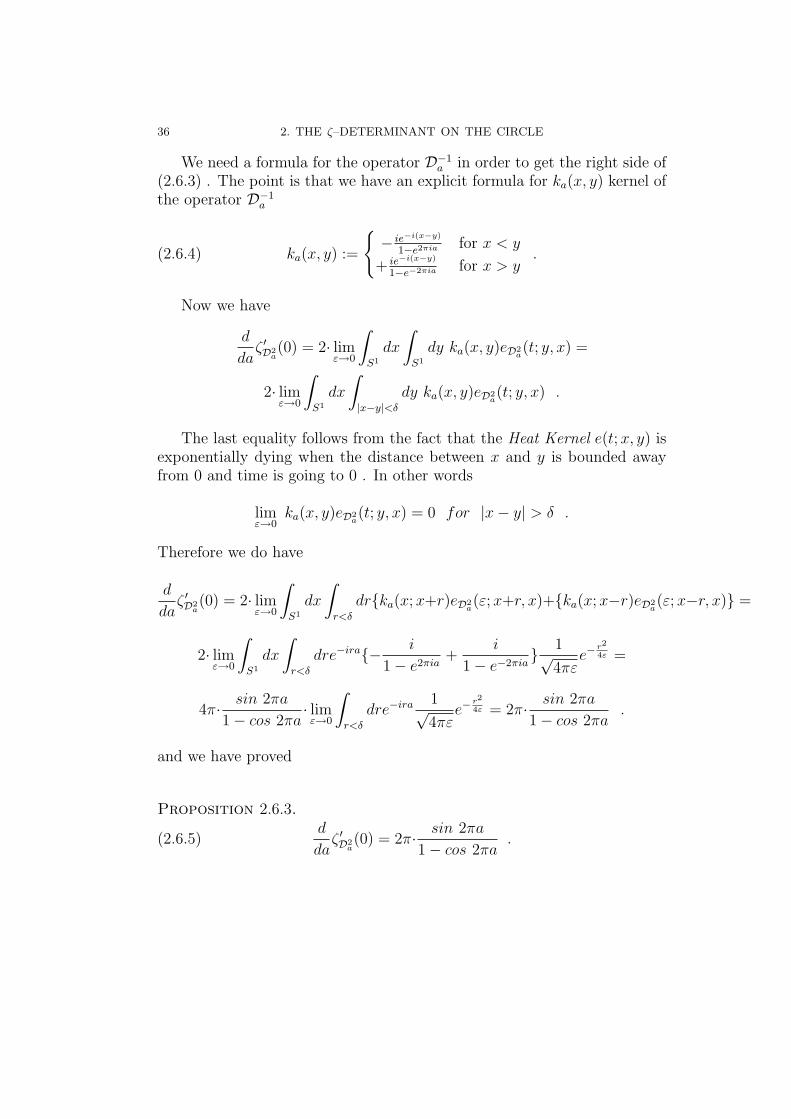
36 2. THE ζ–DETERMINANT ON THE CIRCLE
We need a formula for the operator D−1a in order to get the right side of
(2.6.3) . The point is that we have an explicit formula for ka(x, y) kernel ofthe operator D−1
a
(2.6.4) ka(x, y) :=
{− ie−i(x−y)
1−e2πia for x < y
+ ie−i(x−y)
1−e−2πia for x > y.
Now we have
d
daζ ′D2
a(0) = 2· lim
ε→0
∫S1
dx
∫S1
dy ka(x, y)eD2a(t; y, x) =
2· limε→0
∫S1
dx
∫|x−y|<δ
dy ka(x, y)eD2a(t; y, x) .
The last equality follows from the fact that the Heat Kernel e(t;x, y) isexponentially dying when the distance between x and y is bounded awayfrom 0 and time is going to 0 . In other words
limε→0
ka(x, y)eD2a(t; y, x) = 0 for |x− y| > δ .
Therefore we do have
d
daζ ′D2
a(0) = 2· lim
ε→0
∫S1
dx
∫r<δ
dr{ka(x;x+r)eD2a(ε;x+r, x)+{ka(x;x−r)eD2
a(ε;x−r, x)} =
2· limε→0
∫S1
dx
∫r<δ
dre−ira{− i
1− e2πia+
i
1− e−2πia} 1√
4πεe−
r2
4ε =
4π· sin 2πa
1− cos 2πa· lim
ε→0
∫r<δ
dre−ira 1√4πε
e−r2
4ε = 2π· sin 2πa
1− cos 2πa.
and we have proved
Proposition 2.6.3.
(2.6.5)d
daζ ′D2
a(0) = 2π· sin 2πa
1− cos 2πa.
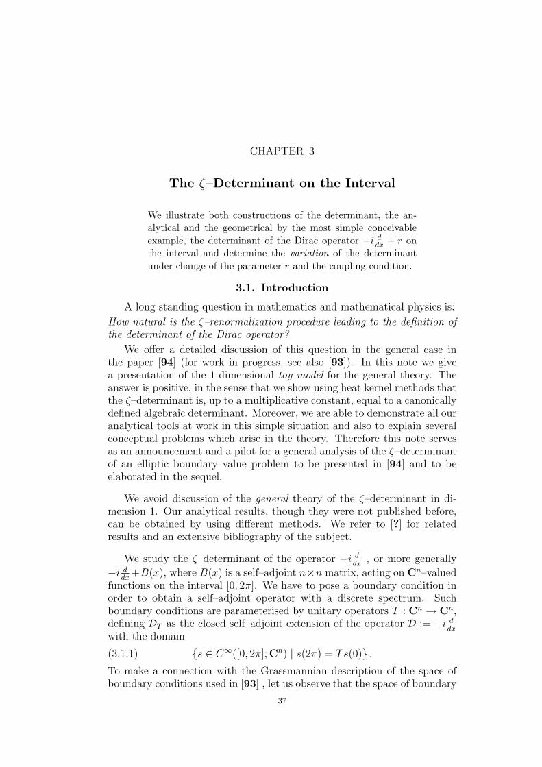
CHAPTER 3
The ζ–Determinant on the Interval
We illustrate both constructions of the determinant, the an-alytical and the geometrical by the most simple conceivableexample, the determinant of the Dirac operator −i d
dx + r onthe interval and determine the variation of the determinantunder change of the parameter r and the coupling condition.
3.1. Introduction
A long standing question in mathematics and mathematical physics is:
How natural is the ζ–renormalization procedure leading to the definition ofthe determinant of the Dirac operator?
We offer a detailed discussion of this question in the general case inthe paper [94] (for work in progress, see also [93]). In this note we givea presentation of the 1-dimensional toy model for the general theory. Theanswer is positive, in the sense that we show using heat kernel methods thatthe ζ–determinant is, up to a multiplicative constant, equal to a canonicallydefined algebraic determinant. Moreover, we are able to demonstrate all ouranalytical tools at work in this simple situation and also to explain severalconceptual problems which arise in the theory. Therefore this note servesas an announcement and a pilot for a general analysis of the ζ–determinantof an elliptic boundary value problem to be presented in [94] and to beelaborated in the sequel.
We avoid discussion of the general theory of the ζ–determinant in di-mension 1. Our analytical results, though they were not published before,can be obtained by using different methods. We refer to [?] for relatedresults and an extensive bibliography of the subject.
We study the ζ–determinant of the operator −i ddx
, or more generally
−i ddx
+B(x), where B(x) is a self–adjoint n×n matrix, acting on Cn–valuedfunctions on the interval [0, 2π]. We have to pose a boundary condition inorder to obtain a self–adjoint operator with a discrete spectrum. Suchboundary conditions are parameterised by unitary operators T : Cn → Cn,defining DT as the closed self–adjoint extension of the operator D := −i d
dxwith the domain
(3.1.1) {s ∈ C∞([0, 2π]; Cn) | s(2π) = Ts(0)} .To make a connection with the Grassmannian description of the space ofboundary conditions used in [93] , let us observe that the space of boundary
37
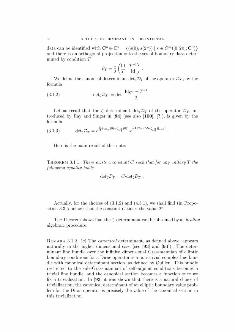
38 3. THE ζ–DETERMINANT ON THE INTERVAL
data can be identified with Cn⊕Cn = {(s(0), s(2π)) | s ∈ C∞([0, 2π]; Cn)}and there is an orthogonal projection onto the set of boundary data deter-mined by condition T
PT =1
2
(Id T−1
T Id
).
We define the canonical determinant detCDT of the operator DT , by theformula
(3.1.2) detCDT := detIdCn − T−1
2.
Let us recall that the ζ–determinant detζDT of the operator DT , in-troduced by Ray and Singer in [84] (see also [100], [?]), is given by theformula
(3.1.3) detζDT = eiπ2
(ηDT(0)−ζD2
T(0))·e−1/2· (d/ds(ζD2
T)|s=0)
.
Here is the main result of this note:
Theorem 3.1.1. There exists a constant C such that for any unitary T thefollowing equality holds
detCDT = C·detζDT .
Actually, for the choices of (3.1.2) and (4.3.1), we shall find (in Propo-sition 3.3.5 below) that the constant C takes the value 2n.
The Theorem shows that the ζ–determinant can be obtained by a “healthy”algebraic procedure.
Remark 3.1.2. (a) The canonical determinant, as defined above, appearsnaturally in the higher dimensional case (see [93] and [94]). The deter-minant line bundle over the infinite–dimensional Grassmannian of ellipticboundary conditions for a Dirac operator is a non-trivial complex line bun-dle with canonical determinant section, as defined by Quillen. This bundlerestricted to the sub–Grassmannian of self–adjoint conditions becomes atrivial line bundle, and the canonical section becomes a function once wefix a trivialization. In [93] it was shown that there is a natural choice oftrivialization; the canonical determinant of an elliptic boundary value prob-lem for the Dirac operator is precisely the value of the canonical section inthis trivialization.
3.1. INTRODUCTION 39
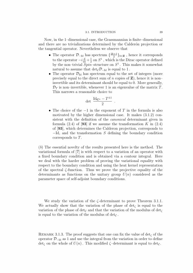
Now, in the 1–dimensional case, the Grassmannian is finite–dimensionaland there are no trivializations determined by the Calderon projection orthe tangential operator. Nevertheless we observe that
• The operator D−Id has spectrum {2k+12}k∈Z , hence it corresponds
to the operator −i ddx
+ 12
on S1 , which is the Dirac operator definedby the non–trivial Spin–structure on S1 . This makes it somewhatnatural to assume that detCD−Id is equal to 1 .• The operator DId has spectrum equal to the set of integers (more
precisely equal to the direct sum of n copies of Z), hence it is non–invertible and its determinant should be equal to 0. More generally,DT is non–invertible, whenever 1 is an eigenvalue of the matrix T .This narrows a reasonable choice to
detIdCn − T±1
2.
• The choice of the −1 in the exponent of T in the formula is alsomotivated by the higher dimensional case. It makes (3.1.2) con-sistent with the definition of the canonical determinant given informula (2.4) of [93] if we assume the transformation K in (2.4)of [93], which determines the Calderon projection, corresponds to−Id, and the transformation S defining the boundary conditioncorresponds to T .
(b) The essential novelty of the results presented here is the method. Thevariational formula of [?] is with respect to a variation of an operator witha fixed boundary condition and is obtained via a contour integral. Herewe deal with the harder problem of proving the variational equality withrespect to the boundary condition and using the heat kernel representationof the spectral ζ-function. Thus we prove the projective equality of thedeterminants as functions on the unitary group U(n) considered as theparameter space of self-adjoint boundary conditions.
We study the variation of the ζ-determinant to prove Theorem 3.1.1.We actually show that the variation of the phase of detζ is equal to thevariation of the phase of detC and that the variation of the modulus of detζ
is equal to the variation of the modulus of detC .
Remark 3.1.3. The proof suggests that one can fix the value of detζ of theoperator D−Id as 1 and use the integral from the variation in order to definedetζ on the whole of U(n) . This modified ζ–determinant is equal to detC.
40 3. THE ζ–DETERMINANT ON THE INTERVAL
In Section 1 we present formulas for the variation of detC. In Section 2we discuss the variation of detζ and, in order to determine the constant C,compute detζ(D−Id).
3.2. The Variation of the Canonical Determinant
In this Section we discuss the variation of detCDT at a fixed boundarycondition T . We replace T by Tr := eirαT , where α = α∗ is a self–adjointn× n matrix and compute
d/dr{detCDTr}|r=0 .
The result is stated in the following Proposition.
Proposition 3.2.1. Let RT (α) denote d/dr{ln detCDTr}|r=0 , then thephase of the variation d/dr{detCDTr}|r=0 is given by the formula
(3.2.1) Im RT (α) = −tr α
2and the modulus is equal to
(3.2.2) Re RT (α) = − i2· tr α(Id + T )(Id− T )−1 .
Proof. We use the formula
(3.2.3)d
dr{ln det Sr} = Tr (
d
dr{Sr}S−1
r ) ,
which in the case Sr := Id−T−1r
2gives
RT (α) = d/dr{ln detCDTr}|r=0 = −i· tr α(Id− T )−1 .
It follows that the phase of the variation of the determinant is equal to
Im RT (α) =1
2i· tr {−iα(Id− T )−1 − (−iα(Id− T )−1)∗}
= −1
2· tr {α(Id− T )−1 + (Id− T−1)−1α}
= −1
2· tr {α(Id− T )−1 − α(Id− T )−1T} = −tr α
2.
We compute the modulus of RT (α) in the same way
Re RT (α) =1
2· tr {−iα(Id− T )−1 + (−iα(Id− T )−1)∗}
= − i2· tr {α(Id− T )−1 − α(Id− T−1)−1} = − i
2· tr α(Id− T )−1(Id + T ) .
�
3.3. THE VARIATION OF THE ζ–DETERMINANT 41
3.3. The Variation of the ζ–Determinant
Now we study the variation of the ζ–determinant under the change ofthe boundary condition described at the beginning of Section 1. We use aunitary twist in order to keep the boundary condition fixed and vary theoperator inside the interval away from the boundary. This method wasused for the first time in this context in [40] and since then has been crucialin obtaining several interesting results in spectral geometry (see [62], [93],[?]). We introduce a smooth cut–off function f : [0, 2π] → [0, 1] equal to 1for 0 ≤ x ≤ π/2 and equal to 0 for 3π/2 ≤ x ≤ 2π and define a unitarytransformation of the (trivial) bundle S1 ×Cn as follows
(3.3.1) Ur(x) := T−1eirf(x)αT .
The operator DTr is unitarily equivalent to the operator
Dr := (Ur(−id
dx)U−1
r )T ,
hence we can compute the variation of the ζ–determinant of DTr by com-puting the variation of the family of operators
Dr = −i ddx− rf ′(x)T−1αT ,
with fixed domain {s | s(2π) = Ts(0)} . Equivalently, we can study theoperator
−i ddx− rf ′(x)T−1αT : C∞(S1;VT )→ C∞(S1;VT ),
where VT denotes the complex bundle over S1 defined by T . Now, we can(as in [93]) directly compute the value of the invariants of the operator Dr
which contribute to the phase. Alternatively, we can use the result fromthe case of closed manifolds, see [45]. In any case we have the followingwell–known result.
Lemma 3.3.1. For any T ∈ U(n) and for any self–adjoint n × n matrix αthe following equalities hold
(3.3.2) ζD2T(0) = 0 and
d
dr{ηDr(0)}|r=0 = −tr α
π.
Corollary 3.3.2. The variation of the phase of detζ is equal to the vari-ation of the phase of detC .
42 3. THE ζ–DETERMINANT ON THE INTERVAL
We need to do more extensive work in order to compute the variationof the modulus of detζ . We have to study the variation of ζ ′D2
T(0) , which is
given by the regularized integral∫ ∞
0
1
t·Tr e−tD2
T dt = lims→0{∫ ∞
0
ts−1·Tr e−tD2T dt−
ζD2T(0)
s} .
Actually, ζD2T(0) vanishes by Lemma 4.3.2 and the integral on the left side
of the identity is well–defined. Now we differentiate with respect to theparameter and obtain
d
dr{ζ ′D2
r(0)}|r=0 =
∫ ∞
0
1
t·Tr(−2tD0D0e
−tD20)dt
= −2
∫ ∞
0
Tr D0D−10 D2
0e−tD2
0dt
= 2
∫ ∞
0
Tr D0D−10
d
dt(e−tD2
0)dt
= 2· limε→0
(Tr D0D−10 e−tD2
0)|t=1/εt=ε = −2· lim
ε→0Tr D0D−1
0 e−εD20 .
This gives us the following formula for the variation of the modulus
(3.3.3)d
dr{−1
2ζ ′D2
r(0)}|r=0 = lim
ε→0Tr D0D−1
0 e−εD20 .
We only need an explicit formula for the kernel of the operator D−10 =
D−1T , to evaluate this formula.
Lemma 3.3.3. Let kT (x, y) denote the kernel of the operator D−1T . Then
kT (x, y) =
{−i(Id− T )−1 for x < y
i(Id− T−1)−1 for x > y .
Now we can evaluate the variation of the modulus of detζ . We have:
d
dr{−1
2ζ ′D2
r(0)}|r=0 = lim
ε→0Tr D0D−1
0 e−εD20
= − limε→0
∫ 2π
0
dx tr(f ′(x)T−1αT
∫ 2π
0
kT (x, y)E(ε; y, x)dy),
where E(ε; y, x) denotes the kernel of the operator e−εD20 . It is immediate
from the properties of the heat kernel that
(3.3.4) limε→0
∫ 2π
0
dx tr(f ′(x)T−1αT
∫{y;|x−y|>σ}
kT (x, y)E(ε; y, x)dy)
= 0
3.3. THE VARIATION OF THE ζ–DETERMINANT 43
for any σ > 0 . Moreover, f ′(x) is equal to 0 for x outside of the interval[π/2, 3π/2] , hence we use Duhamel’s Principle and replace the original heatkernel by the heat kernel of the operator −d2/dx2 on the real line. We have
d
dr{−1
2ζ ′D2
r(0)}|r=0
= − limε→0
∫ 2π
0
dx tr(f ′(x)T−1αT
∫{y;|x−y|<σ}
kT (x, y)E(ε; y, x)dy)
= − limε→0
∫ 2π
0
dx tr(f ′(x)T−1αT{−i(Id− T )−1
∫ σ
0
1√4πε
e−r2/4εdr
+ i(Id− T−1)−1
∫ σ
0
1√4πε
e−r2/4εdr})
= − i√π·∫ 2π
0
tr(f ′(x)T−1αT{(Id− T−1)−1 − (Id− T )−1}
)dx
· limε→0
∫ σ
0
e−r2/4ε dr
2√ε
=i√π·√π
2· tr(T−1αT{(Id− T−1)−1 − (Id− T )−1}
)= − i
2· tr T−1αT (Id− T )−1(Id + T ) .
This ends the proof of Theorem 0.1.
A particular corollary of our computations, which may be of independentinterest, (at least in dimensions higher than 1) is that the only critical pointof the modulus of the determinant is the ‘normalizing’ and ‘diagonalizing’boundary condition given in dimension 1 by T = −Id:
Corollary 3.3.4. The variation of the modulus of the determinants detζ
and detC at T = −Id is equal to 0.
We determine the proportionality constant between detζ and detC by cal-culating the precise value of detζ(DT ) at T = −Id. Recall that by definitiondetC(D−Id) = 1 .
Proposition 3.3.5. For the operator D = −i ddx
acting on Cn–valued func-tions on the interval [0, 2π] we have
detζ(D−Id) = 2n .
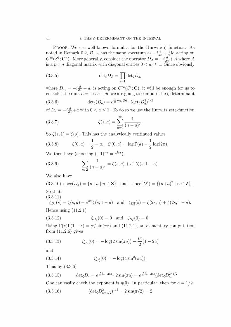
44 3. THE ζ–DETERMINANT ON THE INTERVAL
Proof. We use well-known formulas for the Hurwitz ζ function. Asnoted in Remark 0.2, D−Id has the same spectrum as −i d
dx+ 1
2Id acting on
C∞(S1; Cn). More generally, consider the operator DA = −i ddx
+A where Ais a n×n diagonal matrix with diagonal entries 0 < ai ≤ 1. Since obviously
(3.3.5) detζDA =n∏
i=1
detζDai
where Dai= −i d
dx+ ai is acting on C∞(S1; C), it will be enough for us to
consider the rank n = 1 case. So we are going to compute the ζ determinant
(3.3.6) detζ(Da) = eiπ2
ηDa (0) · (detζD2a)1/2
of Da = −i ddx
+a with 0 < a ≤ 1. To do so we use the Hurwitz zeta-function
(3.3.7) ζ(s, a) =∞∑
n=0
1
(n+ a)s.
So ζ(s, 1) = ζ(s). This has the analytically continued values
(3.3.8) ζ(0, a) =1
2− a, ζ ′(0, a) = log Γ(a)− 1
2log(2π).
We then have (choosing (−1)−s = eiπs):
(3.3.9)∑n∈Z
1
(n+ a)s= ζ(s, a) + eiπsζ(s, 1− a).
We also have
(3.3.10) spec(Da) = {n+a | n ∈ Z} and spec(D2a) = {(n+a)2 | n ∈ Z}.
So that:(3.3.11)ζDa(s) = ζ(s, a) + eiπsζ(s, 1− a) and ζD2
a(s) = ζ(2s, a) + ζ(2s, 1− a).
Hence using (11.2.1)
(3.3.12) ζDa(0) = 0 and ζD2a(0) = 0.
Using Γ(z)Γ(1 − z) = π/ sin(πz) and (11.2.1), an elementary computationfrom (11.2.6) gives
(3.3.13) ζ ′Da(0) = − log(2 sin(πa))− iπ
2(1− 2a)
and
(3.3.14) ζ ′D2a(0) = − log(4 sin2(πa)).
Thus by (3.3.6)
(3.3.15) detζDa = eiπ2
(1−2a) · 2 sin(πa) = eiπ2
(1−2a)(detζD2a)1/2 .
One can easily check the exponent is η(0). In particular, then for a = 1/2
(3.3.16) (detζD2a=1/2)
1/2 = 2 sin(π/2) = 2
3.4. THE OPERATOR −i ddx
+ B(x) - STILL ERRONNEOUS 45
and from (10.2.10) we arrive at 2n for the modulus of the zeta determinantat T = −Id. �
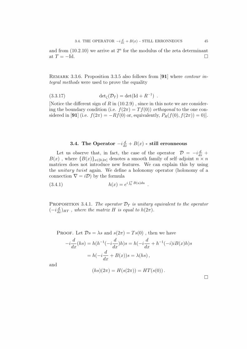
Remark 3.3.6. Proposition 3.3.5 also follows from [91] where contour in-tegral methods were used to prove the equality
(3.3.17) detζ(DT ) = det(Id +R−1) .
[Notice the different sign of R in (10.2.9) , since in this note we are consider-ing the boundary condition (i.e. f(2π) = Tf(0)) orthogonal to the one con-sidered in [91] (i.e. f(2π) = −Rf(0) or, equivalently, PR(f(0), f(2π)) = 0)].
3.4. The Operator −i ddx
+B(x) - still erronneous
Let us observe that, in fact, the case of the operator D = −i ddx
+B(x) , where {B(x)}x∈[0,2π] denotes a smooth family of self–adjoint n × nmatrices does not introduce new features. We can explain this by usingthe unitary twist again. We define a holonomy operator (holonomy of aconnection ∇ = iD) by the formula
(3.4.1) h(x) = ei∫ x0 B(u)du .
Proposition 3.4.1. The operator DT is unitary equivalent to the operator(−i d
dx)HT , where the matrix H is equal to h(2π).
Proof. Let Ds = λs and s(2π) = Ts(0) , then we have
−i ddx
(hs) = h(h−1(−i ddx
)h)s = h(−i ddx
+ h−1(−i)iB(x)h)s
= h(−i ddx
+B(x))s = λ(hs) ,
and(hs)(2π) = H(s(2π)) = HT (s(0)) .
�

CHAPTER 4
EBVP and Grassmannians
4.1. Dirac Operators - Clifford, Compatible Conn., ProductStructure, Index on Closed Mf., Green’s Formula, Calderon
Projector
. . .We now give a more detailed presentation of the situation discussed in
this paper. Let D : C∞(M ;S) → C∞(M ;S) denote a compatible Diracoperator acting on the space of sections of a bundle of Clifford modules Sover compact manifold M with boundary Y . It is not actually necessary toassume that D is a Compatible Dirac Operator. Further technical commentsare made in the final Section of the paper.
In the present paper we always assume that M is an odd-dimensionalmanifold; the even-dimensional case will be discussed separately. And wediscuss only the Product Case. Namely we assume that the Riemannianmetric on M and the Hermitian structure on S are products in a certaincollar neighborhood of the boundary. Let us fix a parameterization N =[0, 1]× Y of the collar. Then in N the operator D has the form
(4.1.1) D = G(∂u +B) ,
where G : S|Y → S|Y is a unitary bundle isomorphism (Clifford multi-plication by the unit normal vector) and B : C∞(Y ;S|Y ) → C∞(Y ;S|Y )is the corresponding Dirac operator on Y , which is an elliptic self-adjointoperator of first order. Furthermore, G and B do not depend on the normalcoordinate u and they satisfy the identities
(4.1.2) G2 = −Id and GB = −BG .
Since Y has dimension 2m the bundle S|Y decomposes into its positive andnegative chirality components S|Y = S+
⊕S− and we have a corresponding
splitting of the operator B into B± : C∞(Y ;S±) → C∞(Y ;S∓) , where(B+)∗ = B− . Equation (7.1.2) can be rewritten in the form(
i 00 −i
)(∂u +
(0 B−
B+ 0
)).
47
48 4. EBVP AND GRASSMANNIANS
4.2. Global Elliptic Boundary Conditions and Grassmannian(s)
In order to obtain an unbounded Fredholm operator with good elliptic reg-ularity properties we have to impose a boundary condition on the opera-tor D . Let Π≥ denote the spectral projection of B onto the subspace ofL2(Y ;S|Y ) spanned by the eigenvectors corresponding to the nonnegativeeigenvalues of B. It is well known that Π≥ is an elliptic boundary condi-tion for the operator D (see [5], [27]). The meaning of the ellipticity is asfollows. We introduce the unbounded operator DΠ≥ equal to the operatorD with domain
dom DΠ≥ = {s ∈ H1(M ;S) ; Π≥(s|Y ) = 0} ,where H1 denotes the first Sobolev space. Then the operator
DΠ≥ = D : dom(DΠ≥)→ L2(M ;S)
is a Fredholm operator with kernel and cokernel consisting only of smoothsections.
The orthogonal projection Π≥ is a pseudodifferential operator of order0 (see [27]). In fact we can take any pseudodifferential operator R of order0 with principal symbol equal to the principal symbol of Π≥ and obtain anoperator DR which satisfies the aforementioned properties.
In order to explain this phenomenon, we give a short exposition of thenecessary facts from the theory of elliptic boundary problems. In contrastto the case of an elliptic operator on a closed manifold, the operator D hasan infinite-dimensional space of solutions. More precisely, the space
{s ∈ C∞(M : S) ; Ds = 0 in M \ Y }
is infinite-dimensional. We introduce Calderon projection, which is theprojection onto H(D) the Cauchy Data space of the operator D
H(D) = {f ∈ C∞(Y ;S|Y ) ; ∃s∈C∞(M ;S) D(s) = 0 in M \ Y and s|Y = f} .
The projection P (D) is a pseudodifferential operator with principal symbolequal to the symbol of Π≥ . It is also an orthogonal projection in thecase of a Dirac operator on an odd-dimensional manifold (see [27]). Theoperator D has the Unique Continuation Property, and hence we have aone to one correspondence between solutions of the operator D and thetraces of the solutions on the boundary Y . This explains roughly, why onlythe projection PR onto the kernel of the boundary conditions R matters.If the difference PR − P (D) is an operator of order −1 , then it followsthat we must choose the domain of the operator DR in such a way thatwe throw away almost all solutions of the operator D on M \ Y , with thepossible exception of a finite dimensional subspace. The above conditionon PR allows us also to construct a parametrix for the operator DR, hence
4.2. GLOBAL ELLIPTIC BOUNDARY CONDITIONS AND GRASSMANNIAN(S) 49
we obtain regularity of the solutions of the operator DR . We refer to themonograph [27] for more details.
We can therefore restrict ourselves to the study of the GrassmannianGr(D) of all pseudodifferential projections which differ from Π≥ by an op-erator of order −1. The space Gr(D) has infinitely many connected compo-nents and two boundary conditions P1 and P2 belong to the same connectedcomponent if and only if
index DP1 = index DP2 .
We are interested, however, in self-adjoint realizations of the operatorD. The involution G : S|Y → S|Y equips L2(Y ;S|Y ) with a symplecticstructure, and Green’s formula (see [27])
(4.2.1) (Ds1, s2)− (s1,Ds2) = −∫
Y
< G(s1|Y ); s2|Y > dy
shows that the boundary condition R provides a self-adjoint realization DR
of the operatorD if and only if ker R is a Lagrangian subspace of L2(Y ;S|Y )(see [26], [27], [40]). We may therefore restrict our attention to those el-ements of Gr(D) which are Lagrangian subspaces of L2(Y ;S|Y ). Moreprecisely, we introduce Gr∗(D), the Grassmannian of orthogonal, pseudo-differential projections P such that P − Π≥ is an operator of order -1 and
(4.2.2) −GPG = Id− P .
The space Gr∗(D) is contained in the connected component of Gr(D) pa-rameterizing projections P with index DP = 0 .
For analytical reasons associated with the existence of the ζ-determinant,in this paper we discuss only the Smooth, Self-adjoint Grassmannian, adense subset of the space Gr∗(D), defined by
(4.2.3) Gr∗∞(D) = {P ∈ Gr∗(D) ; P − Π≥ has a smooth kernel} .
The spectral projection Π≥ is an element of Gr∗∞(D) if and only if ker B ={0} . However, it is well-known that P (D) the (orthogonal) Calderon pro-jection is an element of Gr∗(D) (see for instance [26]), and it was provedby the first author that P (D) − Π≥ is a smoothing operator (see [91],Proposition 2.2.), and hence that P (D) is an element of Gr∗∞(D). Thefinite-dimensional perturbations of Π≥ discussed below (see also [40], [62]and [112]) provide further examples of boundary conditions from Gr∗∞(D) .The latter were introduced by Jeff Cheeger, who called them Ideal BoundaryConditions (see [34], [35]).
50 4. EBVP AND GRASSMANNIANS
For any P ∈ Gr∗(D) the operator DP has a discrete spectrum nicelydistributed along the real line (see [26], [40]). It was shown by the secondauthor that for any P ∈ Gr∗∞(D), ηDP
(s) and ζD2P
(s) are well-defined func-
tions, holomorphic for Re(s) large and with meromorphic extensions to thewhole complex plane with only simple poles. In particular both functionsare holomorphic in a neighborhood of s = 0 . Therefore detζDP defined byformula (??) is a well-defined, smooth function on Gr∗∞(D) (see [113]).
. . .
4.3. Boundary Problems defined by Gr∗∞(D): Inverse Operatorand Poisson Maps
For any P ∈ Gr(D) the operator DP is a Fredholm operator, hence it hasclosed range. As a consequence we can define an inverse to the inducedoperator domDP/ker DP → L2(M ;S)/coker DP . If we assume that Pis an element of Gr∗(D) , the operator DP is self-adjoint and ker DP =coker DP . It follows that if we assume ker DP = {0}, then there exists aninverse D−1
P to the operator DP .
In this section we give an explicit formula for the operator D−1P . This
formula plays a key role in the proof of the main result of the paper. Theoperator D−1
P is a sum of two operators. The first is the interior inverse ofD−1 . The second is a correction term which lives on the boundary.
We start with the ”interior” part of the inverse. Let M = M− ∪Y Mdenote the closed double of the manifold M (M− is a copy of M withreversed orientation). The bundle of Clifford modules S extends to a bundleS of Clifford modules over M and the operator D determines a compatibleDirac operator D over M (equal to D on M and −D on M−). We referto [109], [39] for the details of these constructions and applications to theanalytic realization of K − homology. The operator D : C∞(M ; S) →C∞(M ; S) is an invertible self-adjoint operator, hence its inverse D−1 is awell-defined elliptic operator of order −1 over the manifold M . We alsohave natural extension and restriction maps acting on sections of S and S.The extension (by zero) operator e+ : L2(M ;S) → L2(M ; S) is given bythe formula:
(4.3.1) e+(s) :=
{s on M \M−
0 on M−.
The restriction operator r+ : Hs(M ; S)→ Hs(M ;S) , where Hs denotes the
s − th Sobolev space, is given by f → f = f |M . To simplify the notationin the following we always write
4.3. INVERSE OPERATOR AND POISSON MAPS 51
(4.3.2) D−1 = r+D−1e+ .
The operator D−1 is the interior part of the inverse. It is used in severalcrucial constructions in the theory of boundary problems. It maps L2(M :S) into H1(M ;S), however the range is not necessarily inside the domain ofDP . For this reason we have to introduce an additional term to obtain anoperator with the correct range. To do this, we need to study the situationin a neighborhood of the boundary Y . The restriction of smooth sectionstom the boundary extends to a continuous map:
γ0 : Hs(M ;S)→ Hs− 12 (Y ;S|Y ) ,
which is well-defined for s > 1/2 (see [27]). The corresponding adjointoperator γ∗0 (in the distributional sense) provides us with a well-definedmap
γ∗0 : Hs(Y ;S|Y )→ Hs− 12 (M ;S) ,
for s < −1/2 . Now for any real s the mapping
K = r+D−1γ∗0Γ : C∞(Y ;S|Y )→ C∞(M ;S)
extends to a continuous map K : Hs−1/2(Y ;S|Y ) → Hs(M ;S), with rangeequal to the space
ker(D, s) = {f ∈ Hs(M ;S) : Df = 0 in M \ Y } .
In fact, the map
(4.3.3)K : H(D, s) = Ran{P (D) : Hs−1/2(Y ;S|Y )→ Hs−1/2(Y ;S|Y )} → ker(D, s)
is an isomorphism (see [27]). We have the following equality:
(4.3.4) D−1D = Id−Kγ0 ,
which holds on the space of smooth sections (see [27] Lemma 12.7).
The operator K is called the Poisson operator of D. It defines theCalderon projection:
(4.3.5) P (D) = γ0K
(see [27] Theorem 12.4).
52 4. EBVP AND GRASSMANNIANS
Remark 4.3.1. Formula (4.3.5) gives, a priori, only a projector, not anorthogonal projection, onto H(D) . In the situation discussed in this paper,however, the resulting projector is orthogonal. We refer to [27] for thedetails of the construction, which is originally due to Calderon and Seeley.
To construct the correction term to the parametrix we require that theoperator S(P ) be invertible, but this requirement is equivalent to DP beinginvertibility:
Lemma 4.3.2. The operator DP is an invertible operator if and only if theoperator S(P ) = PP (D) : H(D)→ Ran P is invertible.
Proof. GrassmannianGr∗∞(D) is a subspace of the ”big” GrassmannianGr(D) (see [110], [26], [40] Appendix B). The space Gr(D) has countablymany connected components distinguished by the index of the operatorS(P ), i.e. P1 and P2 belong to the same connected component of Gr(D) ifand only if index S(P1) = index S(P2). The space Gr∗∞(D) is contained inthe index zero component of Gr(D) . Now we have
ker S(P ) = {f : P (D)f = f and P (f) = 0}and
coker S(P ) = {g : Pg = g and P (D)g = 0}
If P is an element of Gr∗(D) , then index S(P ) = index DP = 0 . Wesee that the operator S(P ) is invertible if and only if it has trivial kernel.Similarly a self-adjoint Fredholm operator DP is invertible only if it hastrivial kernel. On the other hand, the operator K defines an isomorphism
K : ker S(P )→ ker DP .
This ends the proof of Lemma. �
Remark 4.3.3. Note that the lemma proves a somewhat stronger state-ment: via the Poisson operator K, constructing solutions for the operatorS(P ) is equivalent to constructing solutions to the elliptic boundary valueproblem DP (and the same for the adjoints). In particular this implies thatthe index of the two operators coincide. This is the underlying reason why
4.3. INVERSE OPERATOR AND POISSON MAPS 53
it is easier to compute determinants on manifolds with boundary than onclosed manifolds.
From now on we assume that DP is invertible. The operator S(P )−1
is not a pseudodifferential operator, as it acts from Ran P into H(D) .However, we can show that it is a restriction of an elliptic pseudodifferentialoperator of order 0. More precisely, the operator PP (D) + (Id − P )(Id −P )(D) is an elliptic pseudodifferential operator, which can be written as
S(P )⊕ (Id− P )(Id− P (D)) : H(D)⊕H(D)⊥ → W ⊕W⊥ ,
where W = Ran P . It can be seen that:
ker S(P ) = coker (Id− P )(Id− P (D))
and
coker S(P ) = ker (Id− P )(Id− P (D)) .
Therefore if we assume that ker S(P ) = {0}, then the operator PP (D) +(Id − P )(Id − P )(D)) is invertible. Its inverse is an elliptic operator (seefor instance [27]) and it follows that
(4.3.6) S(P )−1 = P (D) [PP (D) + (Id− P )(Id− P (D))]−1 P .
We can now present the formula for the inverse of the operator DP .
Theorem 4.3.4. Assume that the operator DP : dom DP → L2(M ;S) isinvertible, then its inverse is given by the formula:
(4.3.7) D−1P = D−1 −KS(P )−1Pγ0D−1 .
Proof. The equality (4.3.3) shows that DK is equal to 0 in M \Y , andhence that DD−1
P is equal to Id on L2(M ;S). Now let f ∈ L2(M ;S), then:
Pγ0(D−1P f) = P (γ0(D−1f)− Pγ0KS(P )−1Pγ0D−1(f) =
P (γ0(D−1f)−PP (D)S(P )−1Pγ0D−1(f) = P (γ0(D−1f)−P (γ0(D−1f) = 0 ,
54 4. EBVP AND GRASSMANNIANS
and hence D−1P f ∈ dom(DP ). We have shown that DPD−1
P : L2(M ;S) →L2(M ;S) is equal to IdL2 and that D−1
P : L2(M ;S)→ dom DP , hence theoperator D−1
P is indeed a right inverse of DP , and obviously it is also a leftinverse. �
Corollary 4.3.5. Let P1, P2 ∈ Gr∗∞(D) such that the operators DP1 andDP2 are invertible. Then the difference D−1
P1− D−1
P2is an operator with
smooth kernel.
Proof. It follows from Theorem 4.3.4 that
(4.3.8) D−1P1−D−1
P2= K(S(P2)
−1P2 − S(P1)−1P1)γ0D−1 .
Now the fact that P1−P2 is an operator with a smooth kernel and equation(4.3.6) implies that the operator S(P2)
−1P2−S(P1)−1P1 also has a smooth
kernel. �
For the rest of this Section we take a closer look at the operator D−1P DP ,
as it allows us to introduce another important operator K(P ) -the Poissonoperator of the operator DP . From formula (4.3.4) we have that
D−1P DP = Id−Kγ0 −KS(P )−1Pγ0(Id−Kγ0) =
Id−Kγ0 +KS(P )−1PP (D)γ0 −KS(P )−1Pγ0 = Id−KS(P )−1Pγ0 .
Hence if f ∈ dom DP , then Pγ0(f) = 0 and
D−1P DPf = (Id−KS(P )−1Pγ0)f = f .
We define the Poisson operator of DP by
(4.3.9) K(P ) = KS(P )−1P ,
which appeared in the second term of the operator D−1P DP and vanishes on
dom DP .
Let g denote an element in the range of the projection P . More precisely,assume that g ∈ Hs(Y ;S|Y ) and Pg = g . Then K(P )g is an element ofker(D, s + 1/2) and hence γ0K(P )g is an element of the space H(D, s), in
4.3. INVERSE OPERATOR AND POISSON MAPS 55
general not equal to g . However, the part of γ0K(P )g along P is in factequal to the original element g :
Pγ0K(P )g = Pγ0KS(P )−1Pg = PP (D)S(P )−1Pg = Pg .
In Section 4 we also need the following result.
Proposition 4.3.6. Let P1, P2 ∈ Gr∗∞(D) such that the operators DP1 andDP2 are invertible. Let f1, f2 ∈ Ran P2 and assume that
P1γ0K(P2)f1 = P1γ0K(P2)f2 .
Then, f1 = f2 and K(P2)f1 = K(P2)f2 .
Proof. We have
P1γ0(K(P2)fi) = S(P1)S(P2)−1fi ,
hence the first equality follows from the invertibility of the operators S(P1)and S(P2). The second is a consequence of the Unique Continuation Prop-erty for Dirac operators. We have
γ0(K(P2)f1 = P (D)S(P2)−1f1 = S(P1)
−1(S(P1)S(P2)−1f1) =
S(P1)−1(S(P1)S(P2)
−1f2) = γ0(K(P2)f2
and hence two solutions of D with the same Cauchy data, hence they areequal. �
Remark 4.3.7. (1) Let us observe that the construction of the inverse pre-sented in this Section gives, in fact, a parametrix for any elliptic boundaryproblem for the Dirac operator. First of all if P is an element of Gr(D)we still can use formula (4.3.7) in order to construct the aforementionedparametrix. The operator S(P )−1 has to be replaced by the operator R(P ), which is of the form
P (D)RP : Ran P → H(D) ,
where R denotes any parametrix of the operator PP (D) + (Id − P )(Id −P (D)) . The formula
56 4. EBVP AND GRASSMANNIANS
CP = D−1 −KR(P )Pγ0D1
now gives the operator, such that DPCP −Id and CPDP −Id have smoothkernels.
(2) More generally, this formula gives a parametrix for any ellipticboundary problem DT as defined in [27] (where the authors were followingSeeley’s exposition [97]). The reason is that NT , the kernel of the boundarycondition T , and H(D) form a Fredholm pair of subspaces of L2(Y ;S|Y ),which allows a parametrix R to be constructed. This fact was well-knownto Booss and Wojciechowski and is implicit in their work [?] and [25] (seealso Proposition 1.4. in [22]. Last but not least, we are not really restrictedin this construction of the parametrix only to Dirac operators. This con-struction holds for any first order elliptic differential operator on a compactmanifold with boundary. The details will be presented elsewhere.
CHAPTER 5
Determinant Line Bundles and the CanonicalDeterminant
5.1. Determinant Bundle
Associated to the family of elliptic boundary value problems {DP : P ∈Gr∞(D)} one has a determinant line bundle DET (D) over Gr∞(D), asexplained in Section 1, which is non-trivial over Gr∞(D). Further for eachchoice of basepoint P0 ∈ Gr∞(D) one has a smooth family of Fredholmoperators
{SP0(P ) := PP0 : Ran P0 → Ran P P ∈ Gr∞(D)}
with associated (Segal) determinant line bundle DETP0 equipped with itscanonical determinant section P → det SP0(P ) ∈ DetP0(P ), whereDetP0(P )is the determinant line of the Fredholm operator SP0(P ). Moreover, forP0, P1 ∈ Gr∞(D) there is a canonical line bundle isomorphism
(5.1.1) DETP0 = DetP0(P1)⊗DETP1 ,
defined where the operators are invertible by
(5.1.2) det [SP1(P )SP0(P1)] = det SP0(P1)⊗ det SP1(P ) .
The first factor on the right-side of (11.1.1) refers to the trivial bundlewith fibre DetP0(P1). The determinant line bundle of the family of ellipticboundary value problems is classified in this sense by
(5.1.3) DET (D) = DETP (D) ,
where P (D) is the Calderon projection, preserving the canonical determi-nant sections
(5.1.4) det DP ←→ det S(P ) ,
where we have written S(P ) for SP (D)(P ). We may therefore rewrite (11.1.1)fibrewise as
57
58 5. DETERMINANT LINE BUNDLES AND THE CANONICAL DETERMINANT
(5.1.5) DET DP = DET DP0 ⊗DetP0(P ) .
We refer to [91] for all these facts.Let σ(DP0) denote the image of the canonical element det SP0(P1) ⊗
det DP0 ∈ DET DP0 ⊗DetP0(P ) under the isomorphism (11.1.5). Relativeto the choice of the basepoint P0, we therefore have two canonical elementsin DET DP , namely det DP and σ(DP0). Thus over the open subset wherethe operators are invertible, according to our earlier discussion we obtaina regularized determinant of DP by taking the quotient of these elements.The point however is to make a canonical choice of the basepoint P0.
In the following, to make the presentation smoother we assume thatker B = {0} . This is in fact not a serious restriction and we can easilyrelax this condition. The point is that now the operators
B± : F± = C∞(Y ;S±)→ F∓ = C∞(Y ;S∓)
are invertible. (We use also F± to denote the space of L2 sections of thebundle of spinors of ”positive′ (resp. ”negative”) chirality.)
Coming back to the canonical choice of the basepoint, in our situationwe are interested just in the real submanifold Gr∗∞(D) of self-adjoint bound-ary conditions and the ‘correct’ choice is indicated by the fact any ellipticboundary condition P ∈ Gr∗∞(D) is described precisely by the property thatits range is the graph of an elliptic unitary isomorphism T : F+ → F−
such that T − (B+B−)−1/2B+ has a smooth kernel.There is a further subtlety that the corresponding orthogonal projection
P+ onto F+ is not actually an element of the Grassmannian. But from(11.1.2) the isomorphism (11.1.5) is well-defined if we include the correc-tion factor τ = det(S(P (D))/det[SP (D)(P
+)SP+(P (D))], which introducesa factor of 1/2 in the final formula (see (5.2.6)). The canonical determinantis then defined to be the quotient taken in DET DP
(5.1.6) detCDP =det DP
σ(DP+).
Roughly speaking this is the quotient det DP/det D+P , the precise definition
takes account of the fact that the domains of the operators DP and D+P
are different and hence that their canonical determinant elements live indifferent complex lines. In Section 1 we carry out a precise computationand we see that detCDP is actually the Fredholm determinant of an operatorliving on the boundary Y constructed from projections P and P (D) .Themain result of the paper is the following Theorem:
5.2. CANONICAL DETERMINANT ON THE GRASSMANNIAN Gr∗∞(D) 59
Theorem 5.1.1. The following equality holds over Gr∗∞(D)
(5.1.7) detζDP = detζDP (D)·detCDP .
Remark 5.1.2. (1) Theorem 11.1.1 shows that, at least on Gr∗∞(D) , theζ-determinant is an object which is a natural extension of the well-definedalgebraic concept of the determinant.
(2) Our results show that the ζ-determinant of the boundary problemDP is actually equal to the Fredholm determinant of the operator S(P )living on the boundary. This extends the corresponding result for the index, which is well-known (see Theorem 20.8 [27]).
(3) With Theorem 11.1.1 at our disposal we can now try a new approachto the pasting formula for the ζ-determinant with respect to a partitioningof a closed manifold. The pasting formula for detC was introduced in [91]. Itis hoped that a new insight into the pasting mechanism of the ζ-determinantwill be obtained by combining results of [91] and formula (11.1.7).
. . .
5.2. Canonical Determinant on the Grassmannian Gr∗∞(D)
In this Section we give a brief review of the construction of the de-terminant line bundle and give an explicit construction of the canonicaldeterminant.
The determinant line bundle over the space of Fredholm operators wasfirst introduced in a seminal paper of Quillen [83]. An equivalent construc-tion which is better suited to our purposes here was subsequently givenby Segal (see [98]), and so we follow his approach. Let Fred(H) denotethe space of Fredholm operators on a separable Hilbert space H. We workfirst in the connected component Fred0(H) of this space parameterizingoperators of index zero. For A ∈ Fred0(H) define
FredA = {S ∈ Fred(H) ; S − A is trace− class} .
Fix a trace-class operator A such that S = A+A is an invertible operator.Then the determinant line of the operator A is defined as
(5.2.1) Det A = FredA ×C/∼= ,
60 5. DETERMINANT LINE BUNDLES AND THE CANONICAL DETERMINANT
where the equivalence relation is defined as follows
(R, z) = (S(S−1R), z) ' (S, z·detFr(S−1R)) .
The Fredholm determinant of the operator S−1R is well-defined, as it is ofthe form IdH plus a trace class operator. Denoting the equivalence class ofa pair (R, z) by [R, z], complex multiplication is defined on Det A by
(5.2.2) λ·[R, z] = [R, λz].
The canonical determinant element is defined by
(5.2.3) det A := [A, 1]
and is non-zero if and only if A is invertible.
The complex lines fit together over Fred0(H) to define a complex linebundle L, the determinant line bundle. To see this, observe first that overthe open set UA in Fred0(H) defined by
UA = {F ∈ Fred0(H) ; F +A is invertible} ,
the assignment F → det F defines a trivializing (non-vanishing) sectionof L|UA . The transition map between the canonical determinant elementsover UA ∩ UB is the smooth (holomorphic) function
gAB(F ) = detFr((F +A)(F + B)−1) .
This defines L globally as a complex line bundle over Fred0(H), endowedwith the canonical section A → det A . If ind A = d we define Det A tobe the determinant line of A ⊕ 0 as an operator H −→ H ⊕ Cd if d > 0, or H ⊕ C−d −→ H if d < 0 and the construction extends in the obviousway to the other components of Fred(H). Note that the canonical sectionis zero outside of Fred0(H).
We use this construction in order to define the determinant line bun-dle over Gr∞(D). For each projection P ∈ Gr∞(D) we have the (Segal)determinant line Det(P (D), P ) of the operator PP (D) : H(D) → Ran Pand the determinant line Det DP of the boundary value problem DP :dom (DP ) −→ L2(M ;S). These lines fit together in the manner explainedabove to define determinant line bundles DETP (D) and DET D, respec-tively, over the Grassmannian (some care has to be taken as the operatoracts between two different Hilbert spaces, but with the obvious notationalmodifications we once again obtain well-defined determinant line bundles).The canonical isomorphism (11.1.3) identifies the two line bundles and pre-serves the determinant elements (equation (11.1.4)). The bundle DETP (D)
5.2. CANONICAL DETERMINANT ON THE GRASSMANNIAN Gr∗∞(D) 61
is a non-trivial line bundle over Gr∞(D), but when restricted to the Grass-mannian Gr∗∞(D) it is canonically trivial.
We use the specific trivialization introduced in [91]. Recall that wework here with orthogonal projections onto the Lagrangian subspaces ofL2(Y ;S|Y ) , which are a compact perturbation of the Cauchy data spaceH(D). We have assumed that ker B = {0}, and hence Π>(B) is an ele-ment of Gr∗∞(D). The range of Π>(B) is actually the graph of the unitaryoperator V> : F+ → F− given by the formula:
V> = (B+B−)−1/2B+ .
This identification extends to the whole Grassmannian Gr∗∞(D): elementsare in 1 − to − 1 correspondence with unitary maps V : F+ → F−, suchthat the difference V − V> is an operator with a smooth kernel. The corre-sponding orthogonal projection P is given by the formula
P =1
2
(IdF+ V −1
V IdF−
).
By choosing a basepoint, the correspondence defined above allows us toestablish an isomorphism between Gr∗∞(D) and the group U∞(F−) of uni-taries acting on F− = L2(Y ;S−) which differ from IdS− by an operatorwith a smooth kernel. It is convenient for us to work with the Calderonprojection as basepoint, hence let K : C∞(Y ;S+)→ C∞(Y ;S−) denote theunitary such that H(D) is equal to the graph(K). Now for any projectionP ∈ Gr∗∞(D) there exists T = T (P ) : F+ → F− such that P = graph(T ),and so we have a natural isomorphism Gr∗∞(D) ∼= U∞(F−) defined by themap P → TK−1 . This is expressed in terms of the homogeneous structureof the Grassmannian by
(5.2.4) P =
(IdF+ 0
0 TK−1
)P (D)
(IdF+ 0
0 KT−1
).
Now we can define a non-vanishing section l of the determinant line bundleDETP (D) over Gr∗∞(D). The value of l at the projection P is the class inDetP (D)(P ) of the couple
(U(P ) =
(IdF+ 0
0 TK−1
); 1) ,
where the operator U(P ) acts from H(D) to Ran(P ). That is, l(P ) =det U(P ). The fact that l(P ) is an element of DetP (D)(P ) ∼= Det DP
follows from the following elementary result.
62 5. DETERMINANT LINE BUNDLES AND THE CANONICAL DETERMINANT
Lemma 5.2.1. The difference between U(P ) and the operator S(P ) = PP (D) :H(D) → RanP is an operator with a smooth kernel, hence det U(P ) =[U(P ), 1] is an element of Det P .
Proof. The operator U(P ) acts from graph(K) = H(D) to graph(T ) =Ran(P ) and acts by(
xKx
)→(IdF+ 0
0 TK−1
)(xKx
)=
(xTx
).
The operator PP (D) is given by the following formula
PP (D) =1
4
(IdF+ + T−1K T−1 +K−1
T +K IdF− + TK−1
),
leading to the following expression for the operator S(P ) = PP (D) :H(D)→ Ran(P )
(5.2.5)
S(P )
(xKx
)=
(IdF++T−1K
2x
IdF−+TK−1
2Kx
)=
(IdF++T−1K
20
0IdF−+TK−1
2
)(xKx
).
Because T−1K (resp. TK−1) differs from IdF+ (resp. IdF+) by a smoothingoperator, it is now obvious that the difference U(P )− S(P ) is an operatorwith a smooth kernel. �
The discussion above allows us to now define the Canonical Determinantover Gr∗∞(D). Let A : H(D) → Ran P denote an invertible Fredholmoperator such that A− S(P ) is an operator of trace class. We have:
det A := [(A, 1)]
= [(U(P )(U(P )−1A), 1)]
= [(U(P ); detFr(U(P )−1A)]
= detFr(U(P )−1A)[(U(P ); 1]
:= detFr(U(P )−1A)·det U(P ) .
where we use equations (5.2.2) and (5.2.2). The above identity means wecan define the determinant of the operator A as the ratio in Det A of thenon-vanishing canonical elements det A and det U(P ), or equivalently asthe Fredholm determinant of the operator U(P )−1A . This leads to thefollowing definition of the Canonical Determinant of the operator DP .
5.2. CANONICAL DETERMINANT ON THE GRASSMANNIAN Gr∗∞(D) 63
Definition 5.2.2. We define the Canonical determinant of the ellipticboundary value problem DP by:
(5.2.6) detCDP := detCS(P ) := detFr (U(P )−1S(P )) ,
where S(P ) := S(P, P (D)).
The essential point is that the determinants of the Fredholm operators DP
and S(P ) regarded as elements of the complex lines Det DP and DetP (D)(P )are canonically identified by the isomorphism (11.1.3). It is straightforwardto check that the Fredholm determinant on the right-side of (5.2.6) is pre-cisely the quotient (11.1.6). In fact, from the proof of Lemma 5.2.1 we seethat the determinant on the right side of the equality (5.2.6) is the Fredholmdeterminant of the operator(
IdF++T−1K
20
0IdF−+TK−1
2
)
acting on the graph of the operator K . Hence we obtain:
Lemma 5.2.3.
(5.2.7) detCDP = detFr
(Id+KT−1
2
),
where the Fredholm determinant on the right-side is taken on F−.
We may therefore reformulate Theorem 11.1.1 as:
Theorem 5.2.4. The following equality holds over Gr∗∞(D)
(5.2.8) detζDP = detζDP (D)·detFrId+KT−1
2,
Equivalently, (since detCDP (D) = 1)
(5.2.9)detζDP
detζDP (D)
=detCDP
detCDP (D)
.
64 5. DETERMINANT LINE BUNDLES AND THE CANONICAL DETERMINANT
Remark 5.2.5. In Section 4 we also use the determinants of operators ofthe form
S(P1)S(P2)−1 : Ran P2 → Ran P1 ,
under the assumption that the operator S(P2) is invertible. It followsfrom the discussion presented above that for any Fredholm operator A :Ran P2 → Ran P1 , such that the difference between the operator A andthe operator P1P2 : Ran P2 → Ran P1 is of trace class we can define thedeterminant of A using the formula
(5.2.10) det A = detFr
(IdF+ 0
0 T2T−11
)A ,
where Ran Pi is equal to graph Ti .
5.3. Canonical Determinant and Metric
. . .
Part 2
Spectral Invariants - The HeatKernel Approach

CHAPTER 6
The Heat Kernel on Gr∞
1
In this chapter we first summarize the basic properties of op-erators with heat kernels, recall the definition of Γ–regularizedspectral functions and invariants, and derive variation formu-las for them. Then we explain Duhamel’s principle and discussvarious simple, but characteristic examples for its application.Also by Duhamel’s principle we establish the ζ–function , theη–function , and the ζ–determinant first for ideal boundaryconditions and subsequently on the smooth self–adjoint Grass-mannian Gr∗∞ (and on Ugraph).
6.1. Introduction
The spectral invariants discussed in this book are constructed from thekernels of the heat operators determined by a Dirac operator D. In thischapter we discuss the construction of the kernels of the operators e−tD 2
P andDe−tD 2
P where DP is a L2–realization of D subject to a boundary conditionP .
Our approach in this book is based on Duhamel’s principle in the spiritof the classical paper of McKean and Singer [67]. The heat kernel is ei-ther constructed from the heat kernel of one or several slightly modified,related operators or it is patched together from heat kernels coming froma decomposition of the manifold into parts. For manifolds with boundaryand with product metric close to the boundary it suffices to glue two heatkernels together, one coming from the interior of the manifold (or from theclosed double) and one coming from a half infinite cylinder over the bound-ary with suitable boundary conditions imposed. The difficulty we face hereis due to the fact that the heat kernels are not local objects and we havethe error term. The good news is that the differences between the preciseand the glued (approximate) heat kernels can be estimated in a sufficientlynice and operational way. The aforementioned estimates allows us to provethe existence of the spectral invariants, we use in the construction of theζ-determinant. Those invariants can be also constructed in a different waysusing parametrix of D. Both methods are essentially equivalent. However,we prefer Duhamel’s principle because it leads us ‘naturally’ to estimates ofthe differences between true and approximate kernels; to estimates about
1Date: November 15, 2001. File name: BOOKHEAT.TEX, uses BOOKC.STY andBOOKREFE.TEX.
67
68 6. THE HEAT KERNEL ON Gr∞ (November 15, 2001)
the true kernels; to formulas and proofs for additivity theorems for spectralinvariants over partitioned manifolds; and to variational formulas.
6.2. Duhamel’s Principle and Heat Kernel Estimates
Let D : C∞(M ;S) → C∞(M ;S) denote a compatible Dirac operatoracting on sections of a bundle of Clifford modules S/ over a compact ma-nifold M (possibly with boundary Y ). Let D0 denote the operator Dd inthe boundaryless case and DP the operator where P is an ideal boundarycondition in the case of a nontrivial boundary Y .
Whenever we can split a manifold into parts we can approximate theheat kernel by the heat kernel of the parts. This follows from Duhamel’sprinciple. More precisely we have
Theorem 6.2.1 (Duhamel’s Formula). Let M be a compact manifold withor without boundary and D : dom(D) → L2(M ; S/) be a L2–extension of anelliptic differential operator with heat kernel e(t;x, x′). Let {U1, U2} be acovering of M by two open submanifolds. For j = 1, 2 we assume that Uj isisometric to an open submanifold of a (not necessarily compact) manifoldMj and that there is given on Mj a L2–extension Dj : dom(Dj)→ L2(Mj; S/j)
of a differential operator with heat kernel ej(t;x, x′) such that Dj and D
coincide over Uj.2 Then there exist positive real constants c1, c2 such that
for any 0 < t < 1
(6.2.1)∣∣∣e(t;x, x′)− ej(t;x, x
′)∣∣∣ < c1e
− c2t for x, x′ ∈ Uj ,
and, more generally,
(6.2.2)∣∣∣e(t;x, x′)−Q(t;x, x′)
∣∣∣ < c1e− c2
t for arbitrary x, x′ ∈M ,
where Q(t;x, x′) is an integral kernel over M obtained by suitably gluing theheat kernels e1 and e2.
Proof. First we define on C∞(M ; S/) for any parameter t > 0 an oper-ator Q(t) with a smooth kernel, given by
Q(t;x, x′) :=2∑
j=1
ψj(x) ej(t;x, x′)ϕj(x
′) ,
where {ϕ1, ϕ2} is a smooth partition of unity on M suitable for the covering{U1, U2} and ψ1, ψ2 are non–negative smooth functions such that
ψj ≡ 1 on {x ∈M | d(x, suppϕj) < δ}and ψj ≡ 0 on {x ∈M | d(x, suppϕj) ≥ 2δ}
2The equality Dj |Uj= D|Uj
is to be understood with regard to the domains.

6.2. DUHAMEL’S PRINCIPLE AND HEAT KERNEL ESTIMATES 69
for a suitable δ > 0. We notice
(6.2.3) dist(suppψ′j, suppϕj) = dist(suppψ′′j , suppϕj) ≥ δ .
Then, for x′ ∈ Uj with ϕj(x′) = 1, we have by definition:
(6.2.4) Q(t;x, x′) =
{ej(t;x, x
′) if d(x, suppϕj) < δ, and
0 if d(x, suppϕj) ≥ 2δ.
For fixed t > 0, we determine the difference between the precise heatkernel e(t;x, x′) and the approximate one Q(t;x, x′). By Duhamel’s Formula(Proposition 6.3.1), we have
e(t;x, x′)−Q(t;x, x′) = −∫ t
0
ds
∫M
dz e(s;x, z)C(t− s; z, x′)
with
C(t− s; z, x′) =
(D2
0 (z) +d
d(t− s)
)Q(t− s; z, x′)
=
(D2
0 (z) −d
ds
)Q(t− s; z, x′)
=2∑
j=1
{ψ′′j (z) ej(t− s; z, x′)ϕj(x
′) + 2ψ′j(z)d
dz(ej(t− s; z, x′))ϕj(x
′)
+ ψj(z)
(D2
0 (z) −d
ds
)ej(t− s; z, x′)︸ ︷︷ ︸
=0
ϕj(x′)}.
As stated in (8.2.5), the supports of ϕj and ψ′j (and, equally, ψ′′j ) aredisjoint and separated from each other by a distance ≥ δ. Then, in finecorrespondence to (6.3.10), the error term C(t − s; z, x′) vanishes both ford(z, x′) < δ and, as well, for sufficiently large geodesic distance, say ifx′ ∈M \ suppϕ2 and z ∈M \ suppϕ1. Moreover, since we have t ≥ s ≥ 0,we obtain
(t− s)−m/2e−c′ d2(z,x′)(t−s) ≤ ct−m/2e−c′ d2(z,x′)
t ≤ ce−c′ d2(z,x′)2t .
Thus we can estimate the first sum
|ψ′′j (z) ej(t− s; z, x′)ϕj(x′)| ≤ c1e
−c′δ2/2t = c1e− c2
t .
Similarly we estimate the second sum. We have
2|ψ′j(z)d
dzej(t− s; z, x′)ϕj(x
′)| ≤ ct−m/2
te−
c′t ≤ c1e
− c2t .
Renaming the constants, we have obtained the crucial estimate
|C(t, x, x′)| < c1e− c2
t for d(x, x′) > δ.
We recall from Lemma 6.2.2 the other crucial estimate
|e(t, x, x′)| < c1e− c2
t .
70 6. THE HEAT KERNEL ON Gr∞ (November 15, 2001)
This gives∣∣e(t;x, x′)−Q(t;x, x′)∣∣ ≤ ∫ t
0
ds
∫M
dz |e(s;x, z)C(t− s; z, x′)|
≤∫ t
0
ds
∫M
dz c1e− c2
t c1e− c2
t = vol(M)c21
∫ t
0
e−c2t
s(t−s) ds
s(t−s)=(t−s)s= 2vol(M)c21
∫ t2
0
e−c2t
s(t−s) ds
t−s≤t/2
≤ 2vol(M)c21
∫ t2
0
e−c2 ts t/2 ds
= 2vol(M)c21
∫ t2
0
e−2c2s ds ≤ 2vol(M)c21e
− 4c2t
∫ t2
0
ds
= vol(M)c21te− 4c2
t < c3e− c4
t .
�
We make a review of the estimates for the kernel e0(t;x, y) of the oper-
ator e0(t) = e−tD02
and E0(t;x, y) the kernel of the operator De−tD02
. Firstof all, there exists positive constants c1 and c2 such that for any 0 < t < 8we have(6.2.5)
‖e0(t;x, y)‖ < c1t−m/2e−c2d2(x,y)/tand‖ E0(t;x, y)‖ < c1t
−(m+1)/2e−c2d2(x,y)/t
The estimate for the heat kernels of the operator DP was proved in[BBKW93] (see [BBKW93], Theorem 22.14) using the variant of the Duha-mel’s principle stated above. In the following we also need estimates, whichimplies vanishing of the heat kernels as time goes to ∞ .
Lemma 6.2.2. There exist positive constants c1 and c2 such that for allx, y ∈M and any t > 0
|E0(t;x, x′)| ≤ c1t
− 1+m2 · e−
t4λ20 · e−c2
d2(x,x′)t ≤ c1t
− 1+m2 · e−c2
d2(x,x′)t ,
where d(x, x′) denotes the geodesic distance. This results holds also for thee0(t, x, y) in the case of the invertible operator D0 (otherwise limit of theoperator e0(t) as t→∞ is equal to the projection onto kernel of D0)
|e0(t;x, x′)| ≤ c1t
−m2 · e−
t4λ20 · e−c2
d2(x,x′)t ≤ c1t
−m2 · e−c2
d2(x,x′)t
Proof. Let {fk;λk}k∈Z denote a discrete spectral resolution of D0 (seealso Remark ??c). We have
|E0(t;x, x′)| ≤
∑k:λk=0
|λk|e−tλ2k · |fk(x)| · |fk(x′)|.
6.3. DUHAMEL’S PRINCIPLE 71
According to the Sobolev Lemma (see for instance [45], Lemma 1.1.4), theimbedding Hm(M ; S/) ↪→ C0(M ; S/) is continuous. Thus we get a uniformpointwise estimate for the eigensections:
(6.2.6) ‖fk(x)‖ ≤ b · (1 + λ2mk ) ,
where the constant b > 0 does not depend on k. Clearly(1 + λ2m
k
m!
)2
≤ e2λ2k .
It follows
|E0(t;x, x′)| ≤ b2
∑k
|λk|e−tλ2k · (1 + λ2m
k )2 ≤ b2(m!)2∑
k
|λk|e−(t−2)λ2k
≤ b1e−(t−4)λ2
0 ·∑
k
e−λ2k ≤ b2e
−(t/2)λ20
for t ≥ 8. Let us observe that there exist positive constants b3, b4, b5 suchthat
tm/2 · e−(t/4)·λ20 ≤ b3 for any 0 < t < +∞,
b4 ≤ e−c2d2(x,x′)
t ≤ b5 for t ≥ 6,
which proves for t ≥ 8 the assertion for the kernel E0 of e−tD20 . In the same
way we prove the assertion for the kernel ε0 . �
6.3. Duhamel’s Principle
In the functional analytical setting, Duhamel’s Principle can be con-sidered as expressing the difference between a given heat kernel and anyarbitrary symmetric integral kernel in the following simple form.
Proposition 6.3.1 (Duhamel’s Formula). Let M be a Riemannian mani-fold with or without boundary and S/ a Hermitian vector bundle over M . LetD0 : domD0 → L2(M ; S/) be an operator with heat kernel(s). Let Q(t;x, x′)be a smooth symmetric kernel for a smooth family of operators of trace classQ(t) such that Q(t; ·, x′) ∈ domD0 for all t > 0 and limt→0Q(t) = Id. Thenwe have for all t > 0, x, x′ ∈M
(6.3.1) e0(t;x, x′) = Q(t;x, x′)
−∫ t
0
ds
∫M
dz e0(s;x, z)
(D2
0(z) +d
d(t− s)
)Q(t− s; z, x′)
= Q(t;x, x′)− (e0 ∗C1)(t;x, x′)
and
(6.3.2) e0(t;x, x′) = Q(t;x, x′) +
∞∑k=1
(−1)k(Q ∗ Ck)(t;x, x′).
72 6. THE HEAT KERNEL ON Gr∞ (November 15, 2001)
Here
(α ∗ β)(t;x, x′) :=
∫ t
0
ds
∫M
dz α(s;x, z)β(t− s; z, x′)
denotes the convolution; and
C1(t) := (D20 +
d
dt)Q(t) with C1(t;x, x
′) := (D20 (x) +
d
dt)Q(t;x, x′)
denotes the error term with the recursive formula
Ck(t) := (C1 ∗ Ck−1)(t) for k > 1.
Note . In (6.3.2), the infinite series of kernels converges uniformly oncompact subsets of R+ ×M ×M and defines an absolute convergent seriesof operators under suitable assumptions about the kernel Q, e.g. when Qitself is a true heat kernel.
Proof. We fix t > 0 and define for s ∈ (0, t] the operator Θ(s) :=e0(s)Q(t− s). Since e0(0) = Q(0) = Id, we have
e0(t)−Q(t) = Θ(t)−Θ(0) =
∫ t
0
d
dsΘ(s)ds
=
∫ t
0
{(d
dse0(s)
)Q(t− s) + e0(s)
d
dsQ(t− s)
}ds
=
∫ t
0
e0(s)
(−D2
0 +d
ds
)Q(t− s)ds,
which proves (6.3.1). To prove (6.3.2) we substitute recursively Q(t) −(e0 ∗C)(t) for e0(t) on the right side of (6.3.1). �
Remark 6.3.2. (a) The preceding proposition remains valid when we re-
place the kernel e0 of e−tD20 by the kernel E0 of the operator D0e
−tD20 . Recall
that E0(t;x, x′) = D0 e0(t;x, x
′). Then equation (6.3.1) has to be replacedby
(6.3.3) E0(t;x, x′) = D0Q(t;x, x′)− (e0 ∗D0C1)(t;x, x
′)
and equation (6.3.2) by
(6.3.4) E0(t;x, x′) = D0Q(t;x, x′) +
∞∑k=1
(−1)k(Q ∗ Ck)(t;x, x′)
with
C1(t;x, x′) := D0C1(t;x, x′) and Ck(t) := (C1 ∗ Ck−1)(t) for k > 1.
(b) To apply Duhamel’s principle a typical situation is met when we want toestimate the difference between the heat kernels e0 and ea of two operators,
6.3. DUHAMEL’S PRINCIPLE 73
say a given D0 and an alternative Da. Clearly (Da + dds
) ea(s) = 0. Thus wecan replace (6.3.1) and (6.3.2) by
(6.3.5) e0 = ea− e0 ∗(D20 −D2
a) ea
and
(6.3.6) e0 = ea− ea ∗(D20 −D2
a) ea + ea ∗(D20 −D2
a) ea ∗(D20 −D2
a) ea− . . .+ (−1)k ea ∗(D2
0 −D2a) ea ∗ · · · ∗ (D2
0 −D2a) ea± . . .
Whenever we can split a manifold into parts we can approximate theheat kernel by the heat kernel of the parts. This follows from Duhamel’sprinciple. More precisely we have
Theorem 6.3.3 (Duhamel’s Splitting Formula). Let M be a compact ma-nifold with or without boundary and D : dom(D) → L2(M ; S/) be a L2–extension of an elliptic differential operator with heat kernel e(t;x, x′). Let{U1, U2} be a covering of M by two open submanifolds. For j = 1, 2 weassume that Uj is isometric to an open submanifold of a (not necessar-ily compact) manifold Mj and that there is given on Mj a L2–extensionDj : dom(Dj) → L2(Mj; S/j) of a differential operator with heat kernel
ej(t;x, x′) such that Dj and D coincide over Uj.
3 Then there exist posi-tive real constants c1, c2 such that for any 0 < t < 1
(6.3.7)∣∣∣e(t;x, x′)− ej(t;x, x
′)∣∣∣ < c1e
− c2t for x, x′ ∈ Uj ,
and, more generally,
(6.3.8)∣∣∣e(t;x, x′)−Q(t;x, x′)
∣∣∣ < c1e− c2
t for arbitrary x, x′ ∈M ,
where Q(t;x, x′) is an integral kernel over M obtained by suitably gluing theheat kernels e1 and e2.
Proof. First we define on C∞(M ; S/) for any parameter t > 0 an oper-ator Q(t) with a smooth kernel, given by
Q(t;x, x′) :=2∑
j=1
ψj(x) ej(t;x, x′)ϕj(x
′) ,
where {ϕ1, ϕ2} is a smooth partition of unity on M suitable for the covering{U1, U2} and ψ1, ψ2 are non–negative smooth functions such that
ψj ≡ 1 on {x ∈M | d(x, suppϕj) < δ}and ψj ≡ 0 on {x ∈M | d(x, suppϕj) ≥ 2δ}
3The equality Dj |Uj= D|Uj
is to be understood with regard to the domains.
74 6. THE HEAT KERNEL ON Gr∞ (November 15, 2001)
for a suitable δ > 0. We notice
(6.3.9) dist(suppψ′j, suppϕj) = dist(suppψ′′j , suppϕj) ≥ δ .
Then, for x′ ∈ Uj with ϕj(x′) = 1, we have by definition:
(6.3.10) Q(t;x, x′) =
{ej(t;x, x
′) if d(x, suppϕj) < δ, and
0 if d(x, suppϕj) ≥ 2δ.
For fixed t > 0, we determine the difference between the precise heatkernel e(t;x, x′) and the approximate one Q(t;x, x′). By Duhamel’s Formula(Proposition 6.3.1), we have
e(t;x, x′)−Q(t;x, x′) = −∫ t
0
ds
∫M
dz e(s;x, z)C(t− s; z, x′)
with
C(t− s; z, x′) =
(D2
0 (z) +d
d(t− s)
)Q(t− s; z, x′)
=
(D2
0 (z) −d
ds
)Q(t− s; z, x′)
=2∑
j=1
{ψ′′j (z) ej(t− s; z, x′)ϕj(x
′) + 2ψ′j(z)d
dz(ej(t− s; z, x′))ϕj(x
′)
+ ψj(z)
(D2
0 (z) −d
ds
)ej(t− s; z, x′)︸ ︷︷ ︸
=0
ϕj(x′)}.
As stated in (8.2.5), the supports of ϕj and ψ′j (and, equally, ψ′′j ) aredisjoint and separated from each other by a distance ≥ δ. Then, in finecorrespondence to (6.3.10), the error term C(t − s; z, x′) vanishes both ford(z, x′) < δ and, as well, for sufficiently large geodesic distance, say ifx′ ∈M \ suppϕ2 and z ∈M \ suppϕ1. Moreover, since we have t ≥ s ≥ 0,we obtain
(t− s)−m/2e−c′ d2(z,x′)(t−s) ≤ ct−m/2e−c′ d2(z,x′)
t ≤ ce−c′ d2(z,x′)2t .
Thus we can estimate the first sum
|ψ′′j (z) ej(t− s; z, x′)ϕj(x′)| ≤ c1e
−c′δ2/2t = c1e− c2
t .
Similarly we estimate the second sum. We have
2|ψ′j(z)d
dzej(t− s; z, x′)ϕj(x
′)| ≤ ct−m/2
te−
c′t ≤ c1e
− c2t .
Renaming the constants, we have obtained the crucial estimate
|C(t, x, x′)| < c1e− c2
t for d(x, x′) > δ.
We recall from Lemma 6.2.2 the other crucial estimate
|e(t, x, x′)| < c1e− c2
t .
6.3. DUHAMEL’S PRINCIPLE 75
This gives∣∣e(t;x, x′)−Q(t;x, x′)∣∣ ≤ ∫ t
0
ds
∫M
dz |e(s;x, z)C(t− s; z, x′)|
≤∫ t
0
ds
∫M
dz c1e− c2
t c1e− c2
t = vol(M)c21
∫ t
0
e−c2t
s(t−s) ds
s(t−s)=(t−s)s= 2vol(M)c21
∫ t2
0
e−c2t
s(t−s) ds
t−s≤t/2
≤ 2vol(M)c21
∫ t2
0
e−c2 ts t/2 ds
= 2vol(M)c21
∫ t2
0
e−2c2s ds ≤ 2vol(M)c21e
− 4c2t
∫ t2
0
ds
= vol(M)c21te− 4c2
t < c3e− c4
t .
�
Remark 6.3.4. For the calculation of the estimation of the poles and thelimiting behaviour of tr(e0(t;x, x)) and tr(E0(t;x, x)) up to an exponentiallysmall error, we shall replace M by Rm and suppose that
D0 = ∆ = − ∂2
∂x21
− · · · − ∂2
∂x2m
far out. This is permissible, because of the preceding Splitting Theorem.Then we consider a coordinate patch U of M and consider it as Rm. Wedefine the alternative operatorDa to beD0 with its coefficients frozen at x′ ∈U and denote the corresponding heat kernel by ea. We denote the differenceD2
0|U − D2a by R. Then we have one more reformulation of Duhamel’s
principle:
(6.3.11) e0(t;x, x′) = ea(t;x, x′)−
∫ t
0
ds
∫Rm
e0(s;x, z)R(z) ea(t−s; z, x′) dz
and
(6.3.12)
e0(t;x, x′) = ea(t;x, x′) +
∞∑k=1
(−1)k
∫ t
0
ds
∫Rm
dz
∫ s
0
ds1
∫Rm
dx1 . . .
. . .
∫ sk−2
0
dsk−1
∫Rm
dxk−1 ea(sk−1;x, xk−1)R(xk−1) ea(sk−2−sk−1;xk−1, xk−2)
. . .R(x1) ea(s− s1;x1, z)R(z) ea(t− s; z, x′).
Example 6.3.5. To give a simple example, we consider the Laplacian ∆0
with domain L2(Rm) and its perturbation ∆1 := ∆0 + V (x) by a potential
76 6. THE HEAT KERNEL ON Gr∞ (November 15, 2001)
V ∈ C∞0 (Rm). Then
e∆0(t;x, x′) = e0(t;x, x
′) = (4πt)−m/2 e−‖x−x′‖2
4t .
Let us assume that e−t∆1 exists. (This is not hard to prove). Then its inte-gral kernel is unique and satisfies the conditions formulated in the Proposi-tion 6.3.1. We apply equation (6.3.12) of the preceding Remark and obtainfor R = V :
e−t∆1 = e−t∆0+∞∑
k=1
(−1)k
∫ t
0
ds
∫ s
0
ds1 . . .
∫ sk−2
0
dsk−1e−sk−1∆0V e−(sk−2−sk−1)∆0 . . .
. . . V e−(s−s1)∆0V e−(t−s)∆0 .
We consider the first term
q0(t;x, x′) =
∫ t
0
e−s∆0 V e−(t−s)∆0 ds.
Setting
Vmax := supRm
|V (x)|
we obtain on the diagonal
|q0(t;x, x)| = |∫ t
0
ds
∫Rm
dz e0(s;x, z)V (z) e0(t− s; z, x)|
≤∫ t
0
ds
∫Rm
dz |e0(s;x, z)V (z) e0(t− s; z, x)|
≤ Vmax
∫ t
0
ds
∫Rm
dz (4πs)−m/2(4π(t− s))−m/2e−‖x−z‖2
4s e−‖x−z‖24(t−s)
≤ Vmax(4π)−m
∫ t
0
(s(t− s))−m/2ds
∫Rm
e−t‖x−z‖24s(t−s) dz.
Since∫Re−x2/α dx =
√πα we have∫
Rm
e−x2/α dx = (πα)m/2 .
Thus we have
|q0(t;x, x)| ≤ Vmax(4π)−mπm/2 ·∫ t
0
(s(t− s))−m/2
(4s(t− s)
t
)m/2
ds
= Vmax4−m/2π−m/2 · t−m/2
∫ t
0
ds =Vmax
(4π)m/2t
2−m2 .
The same type of computations shows that the kernel qk−1(t;x, x) of theoperator ∫ t
0
ds
∫ s
0
ds1 . . .
∫ sk−2
0
dsk−1e−sk−1∆0V . . . V e−(t−s)∆0
6.3. DUHAMEL’S PRINCIPLE 77
is bounded as follows:
|qk−1(t;x, x)| ≤(
Vmax
(4π)m/2
)k1
k!t
2k−m2 .
This proves
Lemma 6.3.6. Let ∆1 := ∆0 + V (x) be a Laplacian with potential V ∈C∞
0 (Rm). Then there exist positive real constants c1, c2 such that for allt > 0 and x ∈ Rm the kernel e1 of the heat operator e−t∆1 can be estimatedby
|e1(t;x, x)| ≤ c1(4πt)m/2
· ec2t

CHAPTER 7
The ζ–Determinant on the Smooth, Self-adjointGrassmannian
In this chapter we discuss the existence of the ζ-determinantof a Dirac operator D on a compact manifold with boundary.We show that the determinant is well defined in the case of theoperator D with a domain determined by a boundary conditionfrom the smooth, self-adjoint Grassmannian Gr∗∞(D).
7.1. Introduction
Recent studies in Quantum Field Theory and Topology have stressedthe importance of the correct definition of the renormalized determinant ofthe Dirac operator over a manifold with boundary. The renormalizationsuccessufully used in the case of a closed manifold is the ζ-renormalizationintroduced by Ray and Singer in [84] (see also [100]). The ζ-determinantof the Dirac operator D on a closed manifold is given by the formula:
(7.1.1) detζD = eiπ2
(ηD(0)−ζD2 (0))·e−1/2·(d/ds(ζD2 (s))|s=0) ,
where ζD2(s) and ηD(s) are functions constructed from the eigenvalues ofthe operator D .
Now let us assume that D : C∞(M ;S) → C∞(M ;S) is a compatibleDirac operator acting on sections of a bundle of Clifford modules S over acompact Riemannian manifold M with boundary Y . We concentrate onthe case of an odd-dimensional manifold M , and from now on we assumethat n = dim M = 2m+ 1 .
Let us point out, however, that our results are true for Dirac operatorson an even-dimensional manifold as well. The necessary modifications dueto the different algebraic structure of the spinors in the odd and even casecan be found in [?], where we discuss the applications of our results in theeven-dimensional situation (see also [22] for an introductory discussion ofapplications of the ζ-determinant of elliptic boundary problems in QuantumChromodynamics).
We discuss only the Product Case. Namely we assume that the Rie-mannian metric on M and the Hermitian structure on S are products in acertain collar neighborhood of the boundary. Let us fix N = [0, 1]× Y thecollar. Then in N the operator D has the form
(7.1.2) D = G(∂u +B)
79
80 7. THE ζ–DETERMINANT ON THE SMOOTH GRASSMANNIAN
where G : S|Y → S|Y is a unitary bundle isomorphism (Clifford multi-plication by the unit normal vector) and B : C∞(Y ;S|Y ) → C∞(Y ;S|Y )is the corresponding Dirac operator on Y , which is an elliptic self-adjointoperator of first order. Furthermore, G and B do not depend on the normalcoordinate u and they satisfy the identities
(7.1.3) G2 = −Id and GB = −BG .
Since Y has dimension 2m the bundle S|Y decomposes into its positive andnegative chirality components S|Y = S+
⊕S− and we have a corresponding
splitting of the operator B into B± : C∞(Y ;S±) → C∞(Y ;S∓) , where(B+)∗ = B− . The equation (7.1.2) can be rewritten in the following form(
i 00 −i
)(∂u +
(0 B−
B+ 0
)).
In order to obtain a nice unbounded Fredholm operator we have to imposea boundary condition on the operator D . Let Π≥ denote the spectralprojection of B onto the subspace of L2(Y ;S|Y ) spanned by the eigenvectorscorresponding to the nonnegative eigenvalues of B. It is well known thatΠ≥ is an elliptic boundary condition for the operator D (see [5], [27]).The meaning of the ellipticity is as follows. We introduce the unboundedoperator DΠ≥ equal to the operator D with domain
dom DΠ≥ = {s ∈ H1(M ;S) ; Π≥(s|Y ) = 0} ,where H1 denotes the first Sobolev space. Then the operator DΠ≥ = D :dom(DΠ≥) → L2(M ;S) is a Fredholm operator with kernel and cokernelconsisting only of smooth sections.
The orthogonal projection Π≥ is a pseudodifferential operator of order0 (see [27]) . In fact we can take any pseudodifferential operator R of order0 with principal symbol equal to the principal symbol of Π≥ and obtain anoperator DR which satisfies the aforementioned properties. Let us point out,however, that only the projection onto the kernel of the operator R is used inthe construction of the operator DR . Therefore we can restrict ourselves tothe study of the Grassmannian Gr(D) of all pseudodifferential projectionswhich differ from Π≥ by an operator of order −1 . The space Gr(D) hasinfinitely many connected components and two boundary conditions P1 andP2 belong to the same connected component if and only if
index DP1 = index DP2 .
We are interested however in self-adjoint realizations of the operator D. The involution G : S|Y → S|Y equips L2(Y ;S|Y ) with a symplecticstructure, and Green’s formula (see [27])
(7.1.4) (Ds1, s2)− (s1,Ds2) = −∫
Y
< G(s1|Y ); s2|Y > dy
7.1. INTRODUCTION 81
shows that the boundary condition R provides a self-adjoint realization DR
of the operatorD if and only if ker R is a Lagrangian subspace of L2(Y ;S|Y )(see [26], [27], [40]). It is therefore reasonable to restrict ourselves to thoseelements of Gr(D) which are Lagrangian subspaces of L2(Y ;S|Y ) . Moreprecisely we introduce Gr∗(D), the Grassmannian of orthogonal, pseudodif-ferential projections P such that P − Π≥ is an operator of order -1 and
(7.1.5) −GPG = Id− P.The space Gr∗(D) is contained in the connected component of Gr(D) pa-rameterizing projections P with index DP = 0 .
We discuss only the Smooth, Self-adjoint Grassmannian, a dense subsetof the space Gr∗(D) , defined by
(7.1.6) Gr∗∞(D) = {P ∈ Gr∗(D) ; P − Π≥ has a smooth kernel} .
Remark 7.1.1. The spectral projection Π≥ is an element of Gr∗∞(D) if andonly if ker B = {0} . However, it is well-known that P (D) the (orthogonal)Calderon projection is an element of Gr∗(D) (see for instance [26]), and ithas been recently observed by Simon Scott (see [91], Proposition 2.2.) thatP (D)−Π≥ is a smoothing operator, and hence that P (D) is an element ofGr∗∞(D) . The finite-dimensional perturbations of Π≥ discussed below (seealso [40], [62] and [112]) provide further examples of boundary conditionsfrom Gr∗∞(D) . The latter were introduced by Jeff Cheeger, who calledthem Ideal Boundary Conditions (see [34], [35]).
For any P ∈ Gr∗(D) the operator DP has a discrete spectrum nicely dis-tributed along the real line (see [26], [40]). Therefore one might expect thatdetζ(DP ) is well defined. To see that, we have to study the asymptotic ex-pansion of the heat kernels involved in the construction of the determinant,or equivalently the expansion of the operator (DP − λ)−1. The existenceof a nice asymptotic expansion of the trace of the heat kernels used in theconstructions of ηDP
(s) and ζD2P
(s) was established in a recent work of Gerd
Grubb [?] . She used the machinery developed in her earlier work and herjoint work with Bob Seeley (see [?], [?], [?]). However, at the moment,the problem of explicit computation of the coefficents in the expansion isopen. From this point of view the existence of the invariants used to definedetζ depends on the vanishing of particular coefficients in the correspondingexpansions.
We choose a different route. It follows from our earlier work on Grass-mannians (see [26], [27], and [40] Appendix B) that Gr∗∞(D) is a path
82 7. THE ζ–DETERMINANT ON THE SMOOTH GRASSMANNIAN
connected space. As a consequence we can perform a Unitary Twist and re-place the operator DP by a unitarily equivalent operator (D+R)Πσ , whereΠσ ∈ Gr∗∞(D) denotes an appropriate finite-dimensional modification ofΠ≥ defined below in Section 1. The operator DΠσ has a well-defined ζ-determinant and the correction term R lives in the collar N . The operatorR is no longer a differential operator, but for any 0 ≤ u ≤ 1 , Ru = R|{u}×Y
is a pseudodifferential operator. If we assume that P − Π≥ has a smoothkernel then the operator Ru has a smooth kernel for each 0 ≤ u ≤ 1 andthis is all that one needs in order to study the correction terms appearing inthe corresponding heat kernels. This is the reason why we restrict attentionto the space Gr∗∞(D). The arguments and the results hold also in the caseof P ∈ Gr∗(D) and P − Π≥ of trace class.
The main result of this chapter is the following Theorem.
Theorem 7.1.2. For any projection P ∈ Gr∗∞(D), ηDP(s) and ζD2
P(s) are
holomorphic functions of s in a neighborhood of s = 0.
Corollary 7.1.3. The ζ-determinant is a well-defined smooth function onGr∗∞(D).
Remark 7.1.4. (1) The result stated above implies the existence of theQuillen ζ-function metric for families of elliptic boundary value problems.This metric was studied before by Piazza [81] in the context of b-calculusdeveloped by Melrose and his collaborators.
(2) In fact, we are able to obtain complete asymptotic expansions of theheat kernels for the operator DP . The reason is that Duhamel’s Principleallows one to study the interior contribution and the boundary contributionseparately and identify the singularities caused by the boundary contribu-tion. This procedure was used before in [40] (Section 4 and Appendix A)and [60] (Section 1). As the asymptotic expansion has been already studied(see [?], [?], [?]) we leave the details to the reader and concentrate insteadon the analysis of the ζ-determinant.
(3) A more difficult problem than the existence of the asymptotic ex-pansion is to show that the invariants used in the construction of the de-terminant are well defined. For instance Grubb and Seeley showed theregularity of the η-function only for finite-dimensional perturbations of the
7.1. INTRODUCTION 83
Atiyah-Patodi-Singer boundary condition (see [?]). A similar result was alsoobtained by Dai and Freed (see [37]). The η-invariant of a more generalclass of boundary problems was also studied recently by Bruning and Lesch(see [?]). There, however, the authors had to deal with the residuum of theη-function at s = 0 , which is not present in our situation.
(4) The results of this chapter were announced in a talk K.P. Wojcie-chowski gave at the Annual Meeting of the AMS in San Francisco in January1995.
We also want to single out one particular result, which is related to thediscussion of the dependence of spectral invariants on the symbol of theoperator given in [?].
Proposition 7.1.5. The value of the ζ-function at s = 0 is constant onGr∗∞(D), i.e.
(7.1.7) ζD2P1
(0) = ζD2P2
(0) .
for any P1, P2 ∈ Gr∗∞(D) .
The results of this chapter allow us to study the ζ-determinant as afunction on Gr∗∞(D) . In particular, we are interested in the relation of theζ-determinant and the Quillen determinant defined as a canonical sectionof the determinant line bundle over the Grassmannian. It was observedby Scott [91] that when restricted to the self-adjoint Grassmannian thedeterminant line bundle over Gr(D) becomes trivial. Moreover, it has anatural trivialization over Gr∗∞(D) . The Quillen determinant expressed inthis trivialization becomes a function. We refer to the determinant obtainedin this way as the canonical determinant and we denote it by detCDP (see[91] for details). In recent work of the author and Simon Scott the relationbetween detζDP and detCDP is studied. In fact, it has been shown that,up to a natural multiplicative constant, the two determinants are equal.Proposition 7.1.5 and Proposition ?? are used in an essential way in theproof of this result. We refer the reader to [?], [23], [93], [94] for details.
In this chapter we discuss another application of Theorem 0.2, the ex-tension of the additivity formula for the η-invariant to boundary condi-tions from Gr∗∞(D). This formula has been previously known only forfinite-dimensional perturbations of the Atiyah-Patodi-Singer condition (see[112]). Let us point out that the additivity formula for the η-invariantstated in Theorem ?? and Proposition 7.1.5 implies the additivity of the
84 7. THE ζ–DETERMINANT ON THE SMOOTH GRASSMANNIAN
phase of the ζ-determinant under the pasting of two manifolds with thesame boundary. This extends the result of Dai and Freed (see [37]).
In the following two sections we study the η-function of DP . We obtainthe following result as a conclusion of our computations.
Theorem 7.1.6. For any P ∈ Gr∗∞(D) the function ηDP(s) is a holomorphic
function of s in the half-plane Re(s) > −1 .
Section 4 contains a discussion of ζD2P
(s) and d/ds(ζD2P
(s))|s=0.
In Section 5 we present proofs of two technical results used in Section 3and Section 4.
7.2. Boundary Contribution to the η-Function. I. Unitary Twistand Duhamel’s Principle
Let us assume for a moment that the manifold M does not have aboundary. The Dirac operator D is then a self-adjoint elliptic operator witha discrete spectrum {λk}k∈Z . We define the η-function of D as follows:
(7.2.1) ηD(s) =∑λk 6=0
sign(λk)|λk|−s .
The function ηD(s) is a holomorphic function of s for Re(s) > dim(M)and it has a meromorphic extension to C with isolated simple poles on thereal axis. The point s = 0 is not a pole and ηD = ηD(0) the η-invariantof the operator D is an important invariant, which has found numerousapplications in geometry, topology and physics. In the case of a compatibleDirac operator D the η-function is actually a holomorphic function of s forRe(s) > −2 . This was shown by Bismut and Freed [17] , who used theheat kernel representation of the η-function
(7.2.2) ηD(s) =1
Γ( s+12
)
∫ ∞
0
ts−12 ·Tr De−tD2
dt ,
which in particular allows us to express the η-invariant as
(7.2.3) ηD(0) =1√π
∫ ∞
0
1√t·Tr De−tD2
dt .
It follows from (7.2.2) that the estimate
|Tr De−tD2| < c√t
7.2. UNITARY TWIST AND DUHAMEL’S PRINCIPLE 85
implies the regularity of the η-function. In fact, Bismut and Freed proveda sharper result: Let E(t;x, y) denote the kernel of the operator De−tD2
,then there exists a positive constant c such that for any x ∈M and for any0 < t < 1
(7.2.4) |tr E(t;x, x)| < c√t .
We argue along the same lines and prove the following Proposition,which implies Theorem 7.1.6.
Proposition 7.2.1. For any P ∈ Gr∗∞(D) there exists a positive constantc > 0 such that for any 0 < t < 1 the following estimate holds
(7.2.5) |Tr DP e−tD2
P | < c .
The proof of Proposition 7.2.1 occupies Section 2 and Section 3 of thechapter. Proposition 7.2.1 is a statement on the small time asymptotics,which by Duhamel’s Principle allows us to replace the kernel of the operatorby a suitable parametrix built from the heat kernel of the operator on M ,the closed double of the manifold M , and the heat kernel of the operatorG(∂u +B) subject to the boundary condition P on a cylinder [0,∞)× Y .
However, we need to start with a concrete representation of the heatkernel on the cylinder. Such a representation is well-known for the originalAtiyah-Patodi-Singer condition Π≥ (see [5], or [27] Section 22). In generalthe projection Π≥ is not an element of the Grassmannian Gr∗∞(D) . Nev-ertheless, one can find easily a finite-dimensional modification of Π≥ whichbelongs to this Grassmannian and then use the explicit formulas for theheat kernel on the cylinder.
We obtain our modification of the Atiyah-Patodi-Singer condition in thefollowing way. The involution G (see (7.1.3)) restricted to ker(B) definesa symplectic structure on this subspace of L2(Y ;S|Y ) and the CobordismTheorem for Dirac Operators (see for instance [27], Corollary 21.16) implies
dim ker(B+) = dim ker(B−) .
The last equality shows the existence of Lagrangian subspaces of ker(B).We choose such a subspace W and let σ : L2(Y ;S|Y )→ L2(Y ;S|Y ) denotethe orthogonal projection of L2(Y ;S|Y ) onto W . Let Π> denote the orthog-onal projection of L2(Y ;S|Y ) onto the subspace spanned by eigenvectors ofB corresponding to the positive eigenvalues. Then
86 7. THE ζ–DETERMINANT ON THE SMOOTH GRASSMANNIAN
(7.2.6) Πσ = Π> + σ ∈ Gr∗∞(D)
gives an element of Gr∗∞(D), which is a finite-dimensional perturbation ofthe Atiyah-Patodi-Singer condition. The operator Dσ = DΠσ is a self-adjoint operator and the properties of its η-function were studied in [40](see Section 4 and Appendix A). It follows that ηDσ(s) is a holomorphicfunction for Re(s) > −2. To make a connection with the operator DP weneed the following result, which is an easy consequence of the topologicalstructure of the Grassmannians studied in [26], [27], [40] (Appendix B).
Lemma 7.2.2. For any P ∈ Gr∗∞(D) there exists a smooth path {gu}0≤u≤1
of unitary operators on L2(Y ;S|Y ) which satisfies
Ggu = guG and gu − Id has a smooth kernel ,
such that g1 = Id and the path {Pu = guΠσg−1u } ⊂ Gr∗∞(D) connects P0 = P
with P1 = Πσ .
We can always assume that the path {gu} is constant on subintervals[0, 1/4] and [3/4, 1] . We introduce U a unitary operator on L2(M ;S) usingthe formula
(7.2.7) U :=
{Id on M \Ngu on N
.
The following Lemma introduces the Unitary Twist, which allows usto replace the operator DP by a modified operator D + R subject to theboundary condition Πσ . This makes possible an explicit construction ofthe heat kernels on a cylinder.
Lemma 7.2.3. The operators DP and DU,σ = (U−1DU)Πσ are unitarilyequivalent operators.
Proof. Let {fk;µk}k∈Z denote a spectral resolution of the operatorDP . This means that for each k we have
Dfk = µkfk and P (fk|Y ) = 0 .
This implies
7.2. UNITARY TWIST AND DUHAMEL’S PRINCIPLE 87
U−1DU(U−1fk) = µk(U−1fk) and Πσ((U−1fk)|Y ) = g−10 P (fk|Y ) = 0 ,
hence {U−1fk;µk} is a spectral resolution of (U−1DU)Πσ .�
In the collar N , we have formulas
U−1DU = D +GU−1∂U
∂u+GU−1[B,U ] ,
and
U−1D2U = D2 − 2U−1∂U
∂u∂u − U−1∂
2U
∂u2+ U−1[B2, U ] ,
which restricted to the collar [0, 1/4]× Y give
(7.2.8) U−1DU = D +GU−1[B,U ] and U−1D2U = D2 + U−1[B2, U ] .
It follows from Lemma 7.2.3 that we can study the operator DU,σ instead ofthe operator DP . We use the representation (7.2.8) in the construction of
the parametrix of the kernel of the operator DU,σe−tD2
U,σ . This parametrix is
built from the heat kernel on the double manifold M and the heat kernel onthe cylinder. The bundle S and the operator D extend to the correspondingobjects S and D on M (see [40]; see [27] for a detailed discussion of theglueing constructions). There is also the obvious double U of the unitarytransformation U . We introduce the operator
U−1DU : C∞(M ; S)→ C∞(M ; S) ,
which is unitarily equivalent to D . Therefore the estimate (7.2.4) holds forthe kernel EU(t;x, y) of the operator
U−1DUe−t(U−1DU)2 = U−1De−tD2
U .
It follows from Duhamel’s Principle that on M \ N up to exponen-
tially small error (in t), the kernel of U−1De−tD2U is equal to the kernel of
DU,σe−tD2
U,σ for 0 < t < 1 (see [40], [60]; see [27] for a detailed discussionof the variant of Duhamel’s Principle we need in this chapter). More pre-cisely, we have the following Lemma, which takes care of the situation inthe interior of M
Lemma 7.2.4. Let EU,σ(t;x, y) denote the kernel of the operator
DU,σe−tD2
U,σ ,
then there exist positive constants c1, c2 such that for any x ∈ M1/8 = M \[0, 1/8]× Y and any 0 < t < 1 the following estimate holds
88 7. THE ζ–DETERMINANT ON THE SMOOTH GRASSMANNIAN
(7.2.9) ‖EU,σ(t;x, x)− EU(t;x, x)‖ ≤ c1e− c2
t .
Hence the estimate (7.2.4) holds for the kernel of the operator DU,σe−tD2
U,σ
in M1/8 .
Now, we study the heat kernel in the collar neighborhood of Y . Onceagain we apply Duhamel’s Principle to replace the kernel EU,σ(t;x, y) of the
operator DU,σe−tD2
U,σ by the corresponding kernel on [0,+∞)×Y . It follows
from equation (7.2.8) that up to an exponentially small error we can usethe kernel of the operator
(7.2.10) (G(∂u +B) +K1)e−t(−∂2
u+B2+K2)σ ,
where
K1 = GU−1[B,U ] and K2 = U−1[B2, U ] .
Let us observe that K1 anticommutes and K2 commutes with the involutionG. The symbol exp(−t(−∂2
u +B2 +K2)σ) in (7.2.10) denotes the followingoperator. We consider the operator G(∂u + B)Πσ on the infinite cylinder[0,+∞)×Y and its square, which we denote by (−∂2
u +B2)σ . The operator(−∂2
u+B2)σ is an unbounded self-adjoint operator in L2([0,+∞)×Y ;S) andthe kernel of the operator exp(−t(−∂2
u +B2)σ) is given by explicit formulas(see [5], [27]). We add the bounded operator K2 and obtain the operator(−∂2
u + B2 + K2)σ . It follows from standard theory (see for instance [86])that the semigroup exp(−t(−∂2
u +B2 +K2)σ) is well defined. We study the
trace of the kernel of (G(∂u +B) +K1)e−t(−∂2
u+B2+K2)σ in the next Section.
7.3. Boundary Contribution to the η-Function. II. Heat Kernelon the Cylinder
In this Section we continue the proof of the Proposition 7.2.1. We haveto show that the boundary contribution to Tr DP e
−tD2P is bounded for t
sufficiently small. Let e(t) denote the operator exp(−t(−∂2u + B2 + K2)σ)
and e1(t) denote the operator exp(−t(−∂2u +B2)σ) . We have the formula
(7.3.1) e(t) = e1(t) +∞∑
n=1
{e1 ∗ K2e1 ∗ K2e1 ∗ ... ∗ K2e1}(t) ,
where the term K2e1 appears n-times in the curly bracket under the sum-mation sign and ∗ denotes convolution (see for instance [27]; Section 22C).
7.3. HEAT KERNEL ON THE CYLINDER 89
It follows from the explicit formulas giving the kernel of the operator e1(t)(see (7.3.5) and Appendix formula (7.5.1)) that∫
Y
tr G(∂u +B)e1(t; (u, y), (v, z))|y=zu=vdy = 0 , y, z ∈ Y .
We want to show that there exists a positive constant C such that for any0 ≤ u ≤ 1/8
(7.3.2) |∫
Y
tr (G(∂u +B) +K1)e(t; (u, y), (v, z))|y=zu=vdy| < C , y, z ∈ Y .
It follows from Formula (7.3.1) that we have to study the trace
∫Y
tr (G(∂u +B) +K1)
{e1 +∞∑
n=1
{e1 ∗ K2e1 ∗ K2e1 ∗ ... ∗ K2e1}}(t; (u, y), (v, z))|y=zu=vdy .
The involution G commutes with the operators e1 and K2 and anticommuteswith B and K1 , which gives us∫
Y
tr GB{e1(t)+∞∑
n=1
{e1 ∗ K2e1 ∗ K2e1 ∗ ... ∗ K2e1}}(t; (u, y), (v, z))|y=zu=vdy = 0 ,
and∫Y
tr K1{e1(t)+∞∑
n=1
{e1 ∗ K2e1 ∗ K2e1 ∗ ... ∗ K2e1}}(t; (u, y), (v, z))|y=zu=vdy = 0 .
Therefore we have the equality
(7.3.3)
∫Y
tr G(∂u +B) +K1)e(t; (u, y), (v, z))|y=zu=vdy =
∫Y
tr G∂u{e1(t)+∞∑
n=1
{e1 ∗ K2e1 ∗ K2e1 ∗ ... ∗ K2e1}}(t; (u, y), (v, z))|y=zu=vdy =
90 7. THE ζ–DETERMINANT ON THE SMOOTH GRASSMANNIAN
∫Y
tr G∂u{∞∑
n=1
{e1 ∗ K2e1 ∗ K2e1 ∗ ... ∗ K2e1}}(t; (u, y), (v, z))|y=zu=vdy .
The last equality in (7.3.3) follows from the fact that∫Y
tr G(∂ue1)(t; (u, y), (v, z))|y=zu=vdy = 0
(see formula (7.5.1)). We have to study the right side of (7.3.3). The crucialpoint here is to estimate the first term∫
Y
tr G(∂ue1) ∗ K2e1(t; (u, y), (v, z))|y=zu=vdy .
We estimate the trace in the Y − direction of the operator
G(∂ue1) ∗ K2e1(t) =
∫ t
0
G(∂ue1(s))K2e1(t− s)ds .
Our result essentially follows from the fact that E1(t − s; (u, y), (v, z)),the kernel of the operator e1(t− s), and F(s; (u, y), (v, z)), the kernel of theoperator ∂ue1(s), have nice ”diagonal” representations on the cylinder. Wecan choose a spectral resolution {ϕn;µn}n∈Z\{0} of the tangential operatorB, such that ϕn corresponds to a positive eigenvalue or is an element ofRan σ and Gϕn = ϕ−n . This means that one has
(7.3.4) Bϕn = µnϕn and Πσϕn = 0
for µn ≥ 0 , and
B(Gϕn) = −µn(Gϕn) and Πσ(Gϕn) = Gϕn .
Now we can represent our kernels in the following way.
(7.3.5) E1(t; (u, y), (v, z)) =∑
n∈Z\{0}
gn(t;u, v)ϕn(y)⊗ϕ∗n(z) ,
and
F(t; (u, y), (v, z)) =∑
n∈Z\{0}
hn(t;u, v)ϕn(y)⊗ϕ∗n(z) ,
where gn(t;u, v) and hn(t;u, v) are given by explicit formulas (see (7.5.1)).We have
TrY G(∂ue1(s))K2e1(t− s)|u=u0=∑
n∈Z\{0}
(G(∂ue1(s))K2e1(t− s)(ϕn);ϕn)|u=u0,
7.3. HEAT KERNEL ON THE CYLINDER 91
and
(∂ue1(s))K2e1(t− s)(ϕn)(y)|u=u0=∑
m∈Z\{0}
∫ ∞
0
dv·gm(s;u0, v)hn(t− s; v, u0)(ϕm;K2ϕn)ϕm(y) .
This gives us the following expressions
(7.3.6) TrY G(∂ue1(s))K2e1(t− s)|u=u0=∑
m∈Z\{0}
∫ ∞
0
h−n(s;u0, v)gn(t− s; v, u0)dv·(ϕn;K2ϕn) ,
and
TrY e1(s)K2e1(t− s)|u=u0=∑
m∈Z\{0}
∫ ∞
0
gn(s;u0, v)gn(t− s; v, u0)dv·(ϕn;K2ϕn) .
The existence of the η-invariant for the operatorDP is now a consequenceof the first part of the following Theorem. The second part of the Theorem isused below in Section 3, where we deal with the ζ-function and its derivative.
Theorem 7.3.1. There exists a positive constant c > 0 such that for anyn 6= 0 and for any 0 < t < 1 we have the following estimates
(7.3.7) |∫ ∞
0
h−n(s;u0, v)gn(t− s; v, u0)dv| <c√
s(t− s),
and
(7.3.8) |∫ ∞
0
gn(s;u0, v)gn(t− s; v, u0)dv| <c√t.
The proof of the Theorem 7.3.1 is completely elementary and consists oflong and tedious computations. We present the proof in the closing sectionof this chapter. Theorem 7.3.1 has the following immediate Corollary.
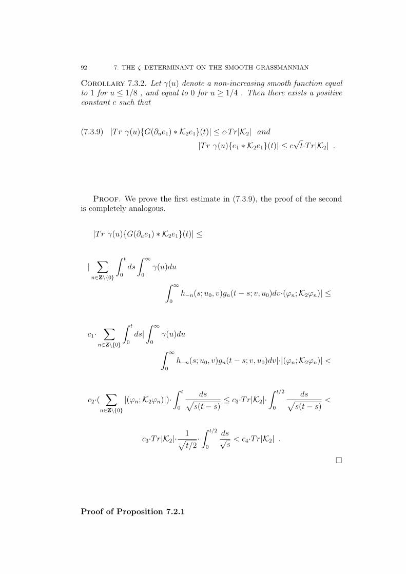
92 7. THE ζ–DETERMINANT ON THE SMOOTH GRASSMANNIAN
Corollary 7.3.2. Let γ(u) denote a non-increasing smooth function equalto 1 for u ≤ 1/8 , and equal to 0 for u ≥ 1/4 . Then there exists a positiveconstant c such that
(7.3.9) |Tr γ(u){G(∂ue1) ∗ K2e1}(t)| ≤ c·Tr|K2| and
|Tr γ(u){e1 ∗ K2e1}(t)| ≤ c√t·Tr|K2| .
Proof. We prove the first estimate in (7.3.9), the proof of the secondis completely analogous.
|Tr γ(u){G(∂ue1) ∗ K2e1}(t)| ≤
|∑
n∈Z\{0}
∫ t
0
ds
∫ ∞
0
γ(u)du
∫ ∞
0
h−n(s;u0, v)gn(t− s; v, u0)dv·(ϕn;K2ϕn)| ≤
c1·∑
n∈Z\{0}
∫ t
0
ds|∫ ∞
0
γ(u)du
∫ ∞
0
h−n(s;u0, v)gn(t− s; v, u0)dv|·|(ϕn;K2ϕn)| <
c2·(∑
n∈Z\{0}
|(ϕn;K2ϕn)|)·∫ t
0
ds√s(t− s)
≤ c3·Tr|K2|·∫ t/2
0
ds√s(t− s)
<
c3·Tr|K2|·1√t/2·∫ t/2
0
ds√s< c4·Tr|K2| .
�
Proof of Proposition 7.2.1
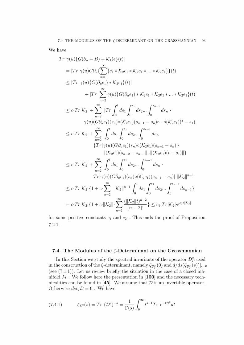
7.4. THE MODULUS OF THE ζ-DETERMINANT ON THE GRASSMANNIAN 93
We have
|Tr γ(u){G(∂u +B) +K1)e}(t)|
= |Tr γ(u)G∂u{∞∑
n=1
{e1 ∗ K2e1 ∗ K2e1 ∗ ... ∗ K2e1}}(t)
≤ |Tr γ(u){G(∂ue1) ∗ K2e1}(t)|
+ |Tr∞∑
n=2
γ(u){G(∂ue1) ∗ K2e1 ∗ K2e1 ∗ ... ∗ K2e1}(t)|
≤ c·Tr|K2|+∞∑
n=2
|Tr∫ t
0
ds1
∫ s1
0
ds2...
∫ sn−1
0
dsn ·
γ(u)(G∂ue1)(sn)◦(K2e1)(sn−1 − sn)◦...◦(K2e1)(t− s1)|
≤ c·Tr|K2|+∞∑
n=2
∫ t
0
ds1
∫ s1
0
ds2..
∫ sn−1
0
dsn
{Tr|γ(u)(G∂ue1)(sn)◦(K2e1)(sn−1 − sn)|·‖(K2e1)(sn−2 − sn−1‖..‖(K2e1)(t− s1)‖}
≤ c·Tr|K2|+∞∑
n=2
∫ t
0
ds1
∫ s1
0
ds2...
∫ sn−1
0
dsn ·
Tr|γ(u)(G∂ue1)(sn)◦(K2e1)(sn−1 − sn)|·‖K2‖n−1
≤ c·Tr|K2|{1 + c·∞∑
n=2
‖K2‖n−1
∫ t
0
ds1
∫ s1
0
ds2...
∫ sn−2
0
dsn−1}
= c·Tr|K2|{1 + c·‖K2‖·∞∑
n=2
(‖K2‖t)n−2
(n− 2)!} ≤ c1·Tr|K2|·ec2t‖K2‖
for some positive constants c1 and c2 . This ends the proof of Proposition
7.2.1.
7.4. The Modulus of the ζ-Determinant on the Grassmannian
In this Section we study the spectral invariants of the operator D2P used
in the construction of the ζ-determinant, namely ζD2P
(0) and d/ds(ζD2P
(s))|s=0
(see (7.1.1)). Let us review briefly the situation in the case of a closed ma-nifold M . We follow here the presentation in [100] and the necessary tech-nicalities can be found in [45]. We assume that D is an invertible operator.Otherwise detζD = 0 . We have
(7.4.1) ζD2(s) = Tr (D2)−s =1
Γ(s)
∫ ∞
0
ts−1Tr e−tD2
dt
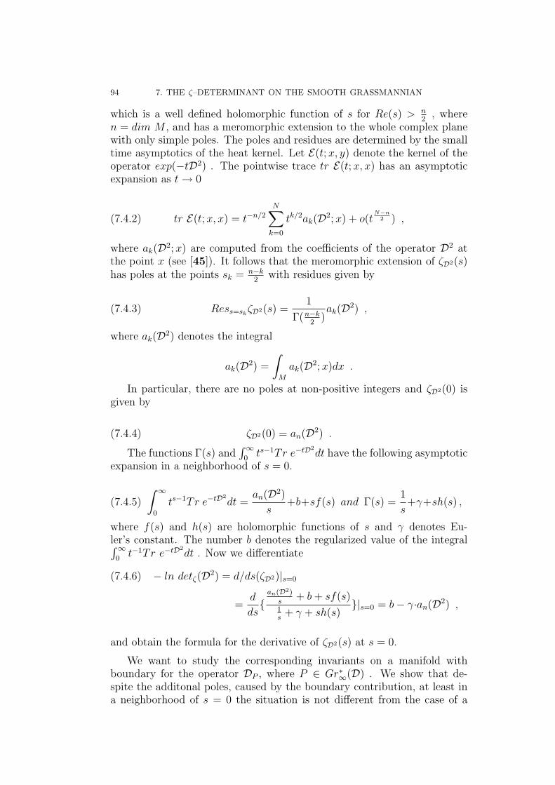
94 7. THE ζ–DETERMINANT ON THE SMOOTH GRASSMANNIAN
which is a well defined holomorphic function of s for Re(s) > n2
, wheren = dim M , and has a meromorphic extension to the whole complex planewith only simple poles. The poles and residues are determined by the smalltime asymptotics of the heat kernel. Let E(t;x, y) denote the kernel of theoperator exp(−tD2) . The pointwise trace tr E(t;x, x) has an asymptoticexpansion as t→ 0
(7.4.2) tr E(t;x, x) = t−n/2
N∑k=0
tk/2ak(D2;x) + o(tN−n
2 ) ,
where ak(D2;x) are computed from the coefficients of the operator D2 atthe point x (see [45]). It follows that the meromorphic extension of ζD2(s)has poles at the points sk = n−k
2with residues given by
(7.4.3) Ress=skζD2(s) =
1
Γ(n−k2
)ak(D2) ,
where ak(D2) denotes the integral
ak(D2) =
∫M
ak(D2;x)dx .
In particular, there are no poles at non-positive integers and ζD2(0) isgiven by
(7.4.4) ζD2(0) = an(D2) .
The functions Γ(s) and∫∞
0ts−1Tr e−tD2
dt have the following asymptoticexpansion in a neighborhood of s = 0.
(7.4.5)
∫ ∞
0
ts−1Tr e−tD2
dt =an(D2)
s+b+sf(s) and Γ(s) =
1
s+γ+sh(s) ,
where f(s) and h(s) are holomorphic functions of s and γ denotes Eu-ler’s constant. The number b denotes the regularized value of the integral∫∞
0t−1Tr e−tD2
dt . Now we differentiate
(7.4.6) − ln detζ(D2) = d/ds(ζD2)|s=0
=d
ds{
an(D2)s
+ b+ sf(s)1s
+ γ + sh(s)}|s=0 = b− γ·an(D2) ,
and obtain the formula for the derivative of ζD2(s) at s = 0.
We want to study the corresponding invariants on a manifold withboundary for the operator DP , where P ∈ Gr∗∞(D) . We show that de-spite the additonal poles, caused by the boundary contribution, at least ina neighborhood of s = 0 the situation is not different from the case of a
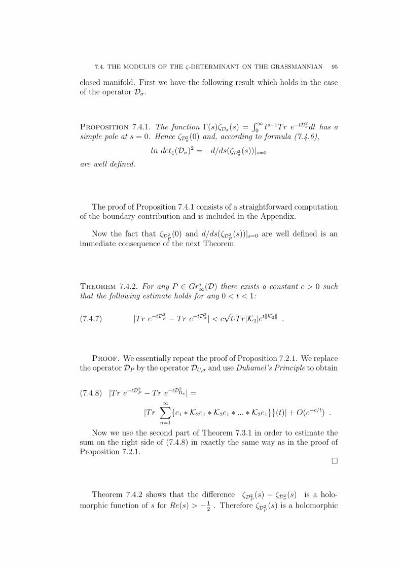
7.4. THE MODULUS OF THE ζ-DETERMINANT ON THE GRASSMANNIAN 95
closed manifold. First we have the following result which holds in the caseof the operator Dσ.
Proposition 7.4.1. The function Γ(s)ζDσ(s) =∫∞
0ts−1Tr e−tD2
σdt has asimple pole at s = 0. Hence ζD2
σ(0) and, according to formula (7.4.6),
ln detζ(Dσ)2 = −d/ds(ζD2σ(s))|s=0
are well defined.
The proof of Proposition 7.4.1 consists of a straightforward computationof the boundary contribution and is included in the Appendix.
Now the fact that ζD2P
(0) and d/ds(ζD2P
(s))|s=0 are well defined is animmediate consequence of the next Theorem.
Theorem 7.4.2. For any P ∈ Gr∗∞(D) there exists a constant c > 0 suchthat the following estimate holds for any 0 < t < 1:
(7.4.7) |Tr e−tD2P − Tr e−tD2
σ | < c√t·Tr|K2|et‖K2‖ .
Proof. We essentially repeat the proof of Proposition 7.2.1. We replacethe operator DP by the operator DU,σ and use Duhamel’s Principle to obtain
(7.4.8) |Tr e−tD2P − Tr e−tD2
Πs | =
|Tr∞∑
n=1
{e1 ∗ K2e1 ∗ K2e1 ∗ ... ∗ K2e1}}(t)|+O(e−c/t) .
Now we use the second part of Theorem 7.3.1 in order to estimate thesum on the right side of (7.4.8) in exactly the same way as in the proof ofProposition 7.2.1.
�
Theorem 7.4.2 shows that the difference ζD2P
(s) − ζD2σ(s) is a holo-
morphic function of s for Re(s) > −12
. Therefore ζD2P
(s) is a holomorphic
96 7. THE ζ–DETERMINANT ON THE SMOOTH GRASSMANNIAN
function of s in a neighborhood of s = 0 . The proof of Theorem 7.1.2 isnow complete.
Proof of Proposition 7.1.5
The Proposition is an easy Corollary of Theorem 7.4.2. It follows from(7.4.1) and (7.4.5) that we have the equality
ζD2P
(0)− ζD2σ(0) = lim
s→0
1
Γ(s)
∫ ∞
0
ts−1Tr(e−tD2P − e−tD2
σ)dt =
lims→0
s
∫ 1
0
ts−1Tr(e−tD2P − e−tD2
σ)dt .
Now we apply Theorem 7.4.2 and obtain
|ζD2P
(0)− ζD2σ(0)| < lim
s→0s
∫ 1
0
ts−1|Tr e−tD2P − Tr e−tD2
σ |dt
< c·lims→0
s
∫ 1
0
ts−1/2dt = 0 .
This ends the Proof of Proposition 7.1.5.
7.5. Proof of Theorem 7.3.1 and Proposition 7.4.1
We start with a discussion of Theorem 7.3.1. Recall the formulas for thefunctions gn(t;u, v) (see for instance [27], (22.33) and (22.35))
(7.5.1) gn(t;u, v) =e−µ2
nt
2√πt·{e−
(u−v)2
4t − e−(u+v)2
4t } for n > 0 ,
and
gn(t;u, v) =e−(−µn)2t
2√πt·{e−
(u−v)2
4t + e−(u+v)2
4t }+
(−µn)e−(−µn)(u+v)·erfc(u+ v
2√t− (−µn)
√t) for n < 0 ,
where
erfc(x) =2√π
∫ ∞
x
e−r2
dr <2√πe−x2
.
We begin with the estimate of the integral∫∞
0gn(s;u0, v)gn(t−s; v, u0)dv
. The most singular term is
7.5. PROOF OF THEOREM AND PROPOSITION 97
∫ ∞
0
e−µ2ns
2√πs·e−
(u0−v)2
4s · e−µ2
n(t−s)
2√π(t− s)
·e−(u0+v)2
4(t−s) dv =
1
4π
e−µ2nt√
s(t− s)
∫ ∞
0
e−t(u0−v)2
4s(t−s) dv <
1
4π
e−µ2nt√
s(t− s)2
√s(t− st
∫ +∞
−∞e−r2
dr =1
2√πte−µ2
nt <1
2√πt
.
We also have the inequality
e−(u+v)2
4t ≤ e−(u−v)2
4t ,
which holds for u, v ≥ 0 and implies the estimate
∫ ∞
0
e−µ2ns
2√πs·e−
(u0∓v)2
4s · e−µ2
n(t−s)
2√π(t− s)
·e−(u0±v)2
4(t−s) dv ≤ 1
2√πt
.
This gives ∫ ∞
0
gn(s;u0, v)gn(t− s; v, u0)dv <1
2√πt
,
for positive n . If n < 0 we also have to discuss the terms of the form
∫ ∞
0
e−µ2ns
2√πs·e−
(u0−v)2
4s ·µneµn(u0+v)·erfc( u0 + v
2√t− s
+ µn
√t− s)dv .
We have
∫ ∞
0
e−µ2ns
2√πs·e−
(u0−v)2
4s ·µneµn(u+v)·erfc( u+ v
2√t− s
+ µn
√t− s) <
µne−µ2
nt
π√s
∫ ∞
0
e−t(u0−v)2
4s(t−s) dv <µne
−µ2nt
√π
√t− st
< ce−µ2nt .
Finally, we have to estimate the term in which the erfc function appearstwice.
98 7. THE ζ–DETERMINANT ON THE SMOOTH GRASSMANNIAN
∫ ∞
0
µneµn(u0+v)erfc(
u0 + v
2√s
+ µn
√s) ·
µneµn(u0+v)erfc(
u0 + v
2√t− s
+ µn
√t− s)dv
<4
π
∫ ∞
0
µ2ne
2µn(u0+v)e−(
u0+v
2√
s+µn
√s)2·e−(
u0+v
2√
t−s+µn
√t−s)2
dv
=4
πµ2
ne−µ2
nt
∫ ∞
0
e−t(u0+v)2
4s(t−s) dv =4
πµ2
ne−µ2
nt2
√s(t− s)
t
∫ +∞
−∞e−r2
dr
≤ 8√πµ2
ne−µ2
nt2√t√π < c
√te−µ2
nt .
The computations given above finish the proof of (7.3.8). We work thesame way in order to obtain the estimate (7.3.7). The only difference is theappearence of hn(t;u0, v) = ∂gn
∂u(t;u0, v) . The first term we have to consider
has the form∫ ∞
0
e−µ2ns
2√πs
|u0 − v|2s
e−(u0−v)2
4s · e−µ2
n(t−s)
2√π(t− s)
e−(u0−v)2
4(t−s) dv <
1
4π
e−µ2nt
2√s(t− s)
∫ ∞
0
|u0 − v|2s
e−(u0−v)2
4s dv =
1
4π
e−µ2nt√
s(t− s){∫ u0
0
u0 − v2s
e−(u0−v)2
4s dv +
∫ ∞
u0
v − u0
2se−
(u0−v)2
4s dv} =
1
4π
e−µ2nt√
s(t− s){∫ u0
0
d(e−(u0−v)2
4s )−∫ ∞
u0
d(e−t(u0−v)2
4s } < e−µ2nt
2π· 1√
s(t− s).
We work on the other terms which appear in∫∞
0h−n(s;u0, v)gn(t−s; v, u0)dv
in the same way. The details are left to the reader.
Now, we show that the function Γ(s)ζDσ(s) has a simple pole at s = 0 .We follow the method applied in Section 4 of [40] to study the η-invariantof Dσ . Let us point out that the situation is simpler in the case of theη-invariant due to the absence of the boundary contribution. Nevertheless,the result corresponding to Lemma 4.2 of [40] holds also in the presentcase. Namely modulo a function holomorphic on the whole complex plane,Γ(s)ζDσ(s) splits into an interior contribution and a cylinder contribution.This again follows from Duhamel’s Principle. First of all,∫ ∞
1
ts−1Tr e−tDσdt
is a holomorphic function on the whole complex plane. For 0 < t < 1,we replace exp(−tD2
σ) by the operator exp(−tD2) inside of M and by the
7.5. PROOF OF THEOREM AND PROPOSITION 99
operator exp(−t(−∂2u + B2)σ) on N . The interior contribution produces
simple poles at the points sk = k−n2
with residues given by the formula∫M
ak(D2;x)dx ,
where D denotes the double of the Dirac operator D on M , the closed doubleof M (see formulas (7.4.2) and (7.4.3)). In particular the contribution tothe residuum at s = 0 is equal to∫
M
an(D2;x)dx = 0 .
This is due to the point-wise vanishing of an(D2;x) , which follows fromthe fact that n = dim M is odd (see for instance [45]). The cylindercontribution has the form
∫ ∞
0
ts−1Tr γ(u)e−t(−∂2u+B2)Πσdt
=∑
n∈Z\{0}
∫ ∞
0
ts−1dt
∫ ∞
0
γ(u)gn(t;u, u)du ,
where γ(u) denotes the cut-off function. The integral∫ ∞
0
ts−1dt
∫ ∞
0
γ(u)gn(t;u, u)du
consists of two terms. The first term produces the contribution∫ ∞
0
ts−1dt{∑
n∈Z\{0}
∫ ∞
0
γ(u)e−µ2
nt
2√πt·(1− sign(n)e−
u2
t )du} .
This is convergent for Re(s) > n/2 and in fact it is equal to
∫ ∞
0
ts−1dt{∑
n∈Z\{0}
∫ ∞
0
γ(u)e−µ2
nt
2√πt·(1− sign(n)e−
u2
t )du} =
∫∞0γ(u)du
2√π·∫ ∞
0
ts−3/2Tr e−tB2
dt .
It follows now from (7.4.2) and (7.4.3) that the expression on the right sidehas a meromorphic extension to the whole complex plane with simple poles.Moreover, it is regular at s = 0 . The reason is that the residuum at s = 0is given by the formula ∫∞
0γ(u)du
2√π
adim(Y )+1(B2) ,
100 7. THE ζ–DETERMINANT ON THE SMOOTH GRASSMANNIAN
and adim(Y )+1(B2) is equal to 0 due to the fact that dim(Y ) + 1 is an odd
number (see for instance [45]). We are left with∫ ∞
0
ts−1dt
∫ ∞
0
γ(u){∑n>0
µne2uµnerfc(
u√t
+ µn
√t)}du .
We only have to show that this term produces at most a simple pole ats = 0 . We can neglect the presence of the cut-off function γ(u) and thenwe obtain for large Re(s)∫ ∞
0
ts−1dt
∫ ∞
0
{∑n>0
µne2uµnerfc(
u√t
+ µn
√t)}du =
1
2
∫ ∞
0
ts−1dt
∫ ∞
0
{∑n>0
d
du(e2uµn)erfc(
u√t
+ µn
√t)}du =
1
2
∫ ∞
0
ts−1dt{∑n>0
{e2uµnerfc(u√t
+ µn
√t)}|∞0 −∫ ∞
0
e2uµn(d
du{erfc( u√
t+ µn
√t)})du} =
1
2
∫ ∞
0
ts−1{∑n>0
e−µ2nt 2√
π(
∫ ∞
0
e−u2/t du√t)−
∑n>0
erfc(µn
√t)}dt =
1
2
∫ ∞
0
ts−1Tr e−tB2
dt− 1
2
∫ ∞
0
ts−1{∑n>0
erfc(µn
√t)}dt .
The first sum on the right side is equal to 12Γ(s)ζB2(s), hence it produces
the correct asymptotic expansion with a simple pole at s = 0 . We needthe next identity in order to deal with the second sum .∫ ∞
0
ts−1erfc(µn
√t)dt =
1
s
∫ ∞
0
d
dt(ts)erfc(µn
√t)dt =
{1
stserfc(µn
√t)}|∞0 −
1
s
∫ ∞
0
tse−µ2nt µn
2√tdt =
− 1
2sµn
∫ ∞
0
ts−1/2e−µ2ntdt = −Γ(s+ 1/2)
2s(µ2
n)−s .
Therefore we obtain
− 1
2
∫ ∞
0
ts−1{∑n>0
erfc(µn
√t)}dt
=Γ(s+ 1/2)
4s
1
2ζB2(s) =
Γ(s+ 1/2)
8sζB2(s) ,
and the expression on the right side has a meromorphic extension to thewhole complex plane, with a simple pole at s = 0 with residuum
7.5. PROOF OF THEOREM AND PROPOSITION 101
Ress=0Γ(s+ 1/2)
8sζB2(s) =
√π
8adim(Y )(B
2) .
We have shown that the cylinder contribution to the trace integral∫∞0ts−1Tr e−tD2
Πσdt has a meromorphic extension to the whole complexplane with an isolated simple pole at s = 0 , which ends the proof of Propo-sition 7.4.1.

Part 3
Pasting of η–Invariants

CHAPTER 8
The Adiabatic Duhamel Principle
1
Let D = D1 ∪ D2 be a compatible Dirac operator on a closedmanifold M which is partitioned M = M1 ∪Y M2 into twocompact manifolds with common boundary Y . Consider itscylindrical prolongation DR = DR
1 ∪ DR2 on the stretched ma-
nifold
MR = M1 ∪ ([−R,R]× Y ) ∪M2 = MR1 ∪MR
2 .
Imposing the Atiyah–Patodi–Singer boundary condition Π> onthe right part M2, we prove a different version of the DuhamelPrinciple and derive an adiabatic formula for the η–invariant
limR→∞
{ηDR
2,Π>(0)−
∫MR
2
ηDR(0;x) dx
}= 0.
Since neither the η–invariant nor the η–density depend, mod-ulo Z, on the length R, we obtain the splitting formula
ηD(0) = ηD1,Π<(0) + ηD2,Π>
(0).
8.1. Introduction
In this and the following chapter, the third part of our book, we derivepasting formulas for the η–invariant . Below, in the fourth part, we thenderive pasting formulas for the determinant line bundle, the ζ–determinant, and for the curvature of the ζ–determinant : how do these invariants splitwhen the manifold is split? One reason for this question is, of course, thatwe wish to understand the invariants of a complicated manifold in terms ofmore simple building blocks.
Various pasting formulas for topological invariants are well–established.The master formula is the Novikov additivity for the signatures of parti-tioned 4k–dimensional manifolds. It can be generalized to additivity theo-rems for the index and to Bojarski type formulas. That are formulas whichgive the index on the closed partitioned manifold in terms of the Cauchydata spaces along the separating hypersurface in even dimension and, cor-respondingly, the spectral flow of a continuous family of Dirac operators interms of the Maslov index of the Cauchy data spaces in odd dimension.
1Date: November 15, 2001. File name: BOOK7C.TEX, uses BOOKC.STY andBOOKREFE.TEX.
105
106 8. THE ADIABATIC DUHAMEL PRINCIPLE (November 15, 2001)
From a topological viewpoint these splitting formulas are not very sur-prising although the precise determination of the correction terms can de-mand considerable effort. The Novikov additivity, for instance, where allcorrection terms are cancelled, is an easy consequence of Poincare dualityand the Mayer–Vietoris sequence of singular homology.
However, analytical explanations for the various additivity formulas forthe index can also be obtained. They help to understand the nature ofthe correction terms. Here the master problem is the Riemann–Hilbertproblem of complex analysis, expressing the index of a coupling problemalong a curve solely by the coupling data.
Unfortunately, we need a little more topology, differential geometry,functional analysis, and elliptic partial differential equation analysis whenwe base our pasting laws on the decomposition of a given closed manifoldinto two manifolds with boundary (that is the analytical approach) insteadof basing the calculations on triangulations of the manifold (as it is the sin-gular homology’s approach). The benefit of the analytical approach is thatwe can describe and follow the cutting and pasting process explicitly on thelevel of the operators and their eigenvalues and not only on the level of thehomology groups and their invariants.
By now, it seems that splitting formulas for the index are rather wellunderstood. The reason is that the index is given by a local formula andthe splitting is rather obvious as soon as the process of cutting and pastingof operators is understood. To understand the underlying idea it sufficesto read the concluding Chapter 26 of our monograph [27]. One majortopic of that book has been the cutting and pasting of Dirac operatorsover partitioned manifolds and the various corresponding index additivitytheorems.
For a different approach we refer to the work by N. Teleman (see, inparticular, [103], [104]) and others on a true discretisation of the Diracoperator over a triangulated manifold. These authors carry out the analysisin intimate analogy to the topology. The discrete methods have been provedsuccessful in some instances (see e.g. Muller [72] and Luck [63]), but adiscrete description of spectral and other global elliptic boundary conditionsand the corresponding calculation of topological and spectral invariants ismissing (1997).
Splitting formulas for spectral quantities like the η–invariant and thedeterminant which are not topological invariants are a veritable challenge.Surprisingly, here the process of understanding was running in reverse order.First the analysis was understood, i.e. the additivity of the η–invariant, laterthe underlying procedure of algebraic topology, i.e. the pasting formula forthe canonical determinant. All that will be explained in the following.
In this chapter we shall use the following notations and make the fol-lowing assumptions.
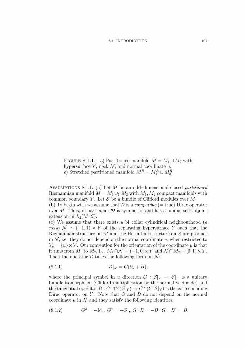
8.1. INTRODUCTION 107
Figure 8.1.1. a) Partitioned manifold M = M1 ∪M2 withhypersurface Y , neck N , and normal coordinate u.b) Stretched partitioned manifold MR = MR
1 ∪MR2
Assumptions 8.1.1. (a) Let M be an odd–dimensional closed partitionedRiemannian manifold M = M1∪Y M2 with M1,M2 compact manifolds withcommon boundary Y . Let S be a bundle of Clifford modules over M .(b) To begin with we assume that D is a compatible (= true) Dirac operatorover M . Thus, in particular, D is symmetric and has a unique self–adjointextension in L2(M ;S).(c) We assume that there exists a bi–collar cylindrical neighbourhood (aneck) N ' (−1, 1) × Y of the separating hypersurface Y such that theRiemannian structure on M and the Hermitian structure on S are productinN , i.e. they do not depend on the normal coordinate u, when restricted toYu = {u}×Y . Our convention for the orientation of the coordinate u is thatit runs from M1 to M2, i.e. M1∩N = (−1, 0]×Y and N ∩M2 = [0, 1)×Y .Then the operator D takes the following form on N :
(8.1.1) D|N = G(∂u +B),
where the principal symbol in u–direction G : S|Y → S|Y is a unitarybundle isomorphism (Clifford multiplication by the normal vector du) andthe tangential operator B : C∞(Y ;S|Y )→ C∞(Y ;S|Y ) is the correspondingDirac operator on Y . Note that G and B do not depend on the normalcoordinate u in N and they satisfy the following identities
(8.1.2) G2 = −Id , G∗ = −G , G ·B = −B ·G , B∗ = B.
108 8. THE ADIABATIC DUHAMEL PRINCIPLE (November 15, 2001)
Hence, G is a skew–adjoint involution and S, the bundle of spinors, decom-poses in N into ±i–eigenspaces of G, S|N = S+⊕S−. It follows that (8.1.1)leads to the following representation of the operator D in N
(8.1.3) D|N =
(i 00 −i
)·(∂u +
(0 B− = B∗
+
B+ 0
)),
where B+ : C∞(Y ;S+)→ C∞(Y ;S−) maps the spinors of positive chiralityinto the spinors of negative chirality.(d) To begin with we consider only the case of kerB = {0}. That impliesthat B is an invertible operator. More precisely, there exists a pseudo–differential elliptic operator L of order −1 such that BL = IdS = LB (see,for instance, [27], Proposition 9.5).(e) For real R > 0 we study the closed stretched manifold MR which weobtain from M by inserting a cylinder of length 2R, i.e. replacing the collarN by the cylinder (−2R− 1,+1)× Y
MR = M1 ∪ ([−2R, 0]× Y ) ∪M2 .
We extend the bundle S to the stretched manifold MR in a natural way. Theextended bundle will be also denoted by S. The Riemannian structure onM and the Hermitian structure on S are product in N , hence we can extendthem to smooth metrics on MR in a natural way and, at the end, we canextend the operator D to an operator DR on MR by using formula (8.1.1).Then MR splits into two manifolds with boundary: MR = MR
1 ∪MR2 with
MR1 = M1∪
((−2R,R]×Y
), MR
2 =([−R, 0)×Y
)∪M2, and ∂M1 = ∂MR
2 =
{−R} × Y . Consequently, the operator DR splits into DR = DR1 ∪ DR
2 . Weshall impose spectral boundary conditions to obtain self–adjoint operatorsD1,Π< , DR
1,Π<, D2,Π> , and DR
2,Π>in the corresponding L2 spaces on the parts
(see (8.1.4)).(f) We also introduce the complete, non–compact Riemannian manifold withcylindrical end
M∞2 :=
((−∞, 0]× Y
)∪M2
by gluing the half–cylinder (−∞, 0] × Y to the boundary Y of M2.Clearly, the Dirac operator D extends also to C∞(M∞
2 ,S).
To fix our notation we recall from part II of this book. Let Π> (re-spectively Π<) denote the spectral projection of B onto the subspace ofL2(Y ;S|Y ) spanned by the eigensections corresponding to the positive (re-spectively negative) eigenvalues. Then Π> is a self–adjoint elliptic bound-ary condition for the operator D2 = D|M2 (see [27], Proposition 20.3). Thismeans that the operator D2,Π> defined by
(8.1.4)
{D2,Π> = D|M2
dom(D2,Π>) = {s ∈ H1(M2;S|M2) | Π>(s|Y ) = 0}
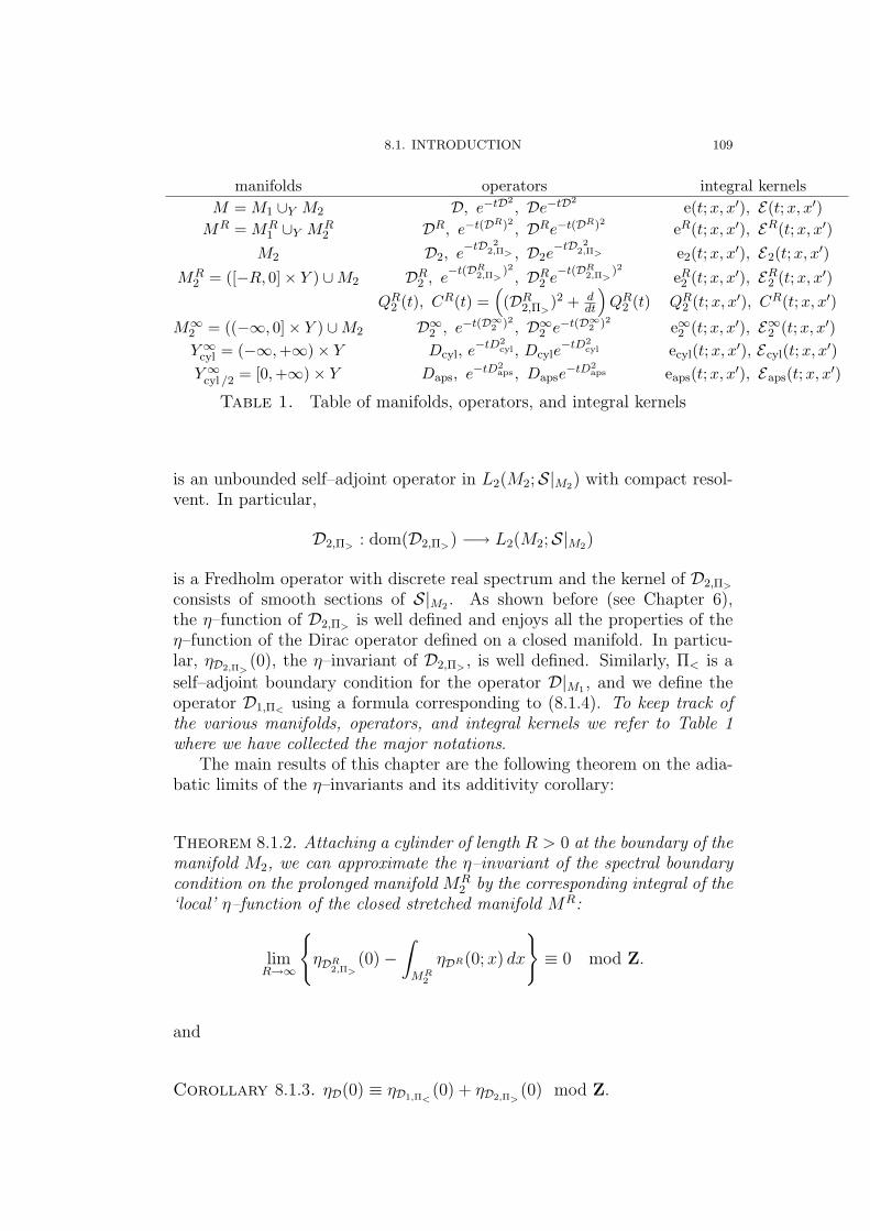
8.1. INTRODUCTION 109
manifolds operators integral kernelsM = M1 ∪Y M2 D, e−tD2
, De−tD2e(t;x, x′), E(t;x, x′)
MR = MR1 ∪Y MR
2 DR, e−t(DR)2 , DRe−t(DR)2 eR(t;x, x′), ER(t;x, x′)M2 D2, e
−tD 22,Π> , D2e
−tD 22,Π> e2(t;x, x′), E2(t;x, x′)
MR2 = ([−R, 0]× Y ) ∪M2 DR
2 , e−t(DR
2,Π>)2
, DR2 e
−t(DR2,Π>
)2 eR2 (t;x, x′), ER
2 (t;x, x′)QR
2 (t), CR(t) =((DR
2,Π>)2 + d
dt
)QR
2 (t) QR2 (t;x, x′), CR(t;x, x′)
M∞2 = ((−∞, 0]× Y ) ∪M2 D∞2 , e−t(D∞2 )2 , D∞2 e−t(D∞2 )2 e∞2 (t;x, x′), E∞2 (t;x, x′)Y ∞
cyl = (−∞,+∞)× Y Dcyl, e−tD2cyl , Dcyle
−tD2cyl ecyl(t;x, x′), Ecyl(t;x, x′)
Y ∞cyl /2 = [0,+∞)× Y Daps, e−tD2
aps , Dapse−tD2
aps eaps(t;x, x′), Eaps(t;x, x′)
Table 1. Table of manifolds, operators, and integral kernels
is an unbounded self–adjoint operator in L2(M2;S|M2) with compact resol-vent. In particular,
D2,Π> : dom(D2,Π>) −→ L2(M2;S|M2)
is a Fredholm operator with discrete real spectrum and the kernel of D2,Π>
consists of smooth sections of S|M2 . As shown before (see Chapter 6),the η–function of D2,Π> is well defined and enjoys all the properties of theη–function of the Dirac operator defined on a closed manifold. In particu-lar, ηD2,Π>
(0), the η–invariant of D2,Π> , is well defined. Similarly, Π< is a
self–adjoint boundary condition for the operator D|M1 , and we define theoperator D1,Π< using a formula corresponding to (8.1.4). To keep track ofthe various manifolds, operators, and integral kernels we refer to Table 1where we have collected the major notations.
The main results of this chapter are the following theorem on the adia-batic limits of the η–invariants and its additivity corollary:
Theorem 8.1.2. Attaching a cylinder of length R > 0 at the boundary of themanifold M2, we can approximate the η–invariant of the spectral boundarycondition on the prolonged manifold MR
2 by the corresponding integral of the‘local’ η–function of the closed stretched manifold MR:
limR→∞
{ηDR
2,Π>(0)−
∫MR
2
ηDR(0; x) dx
}≡ 0 mod Z.
and
Corollary 8.1.3. ηD(0) ≡ ηD1,Π<(0) + ηD2,Π>
(0) mod Z.
110 8. THE ADIABATIC DUHAMEL PRINCIPLE (November 15, 2001)
Remark 8.1.4. With hindsight, it is not surprising that modulo the inte-gers the preceding additivity formula for the η–invariant on a partitionedmanifold is precise. An intuitive argument runs along the following lines:‘almost’ all eigensections and eigenvalues of the operator D on the closedpartitioned manifold M = M1 ∪ M2 can be traced back either to eigen-sections ψ1,k and eigenvalues µ1,k of the spectral boundary problem D1,Π<
on the part M1 or to eigensections ψ2,` and eigenvalues µ2,` of the spectralboundary problem D2,Π> on the part M2. Unfortunately, we have no explicitmethod for doing an exact correspondence. But we have an approximatemethod: due to the product form of the Dirac operator in a neighbourhoodof the separating hypersurface, eigensections on one part M1 or M2 of themanifold M can be extended to smooth sections on the whole of M . Not astrue eigensections of D, but with a relative error which is rapidly decreasingwith R → ∞ when we attach cylinders of length R to the part manifoldsor, equivalently, insert a cylinder of length 2R in M . So much about thegreat majority of eigensections and eigenvalues.
There is also a residual set {µ0,j} of eigenvalues of D which can neitherbe traced back to eigenvalues of D1,Π< nor of D2,Π> . These eigenvaluescan, however, be traced back to the kernel of the Dirac operators D∞1 andD∞2 on the part manifolds with cylindrical ends M∞
1 and M∞2 . Because of
Fredholm properties the residual set is finite and, hence (by Appendix 2)can be discarded for calculating the η–invariant .
Therefore no R, no prolongation of the bicollar neighbourhood N entersthe formula. Nevertheless, our arguments rely on an adiabatic argument tostrain the spectrum of D into its three parts
(8.1.5) specD ∼ {µ0,j} ∪ {µ1,k} ∪ {µ2,`}.
For the most part of this chapter, however, we shall not make all argumentsexplicit on the level of the single eigenvalue. It suffices to keep to the levelof the η–invariant . Roughly speaking, the reason is the following. Con-trary to the index, the η–invariant can not be described by a local formula.Nevertheless, it can be described by an integral over the manifold. Theintegrand, however, is not defined in local terms solely. In particular, whenwriting the η–function in integral form and decomposing the η–integral
ηD(s) =
∫M
ηD(s;x, x) dx =
∫M1
ηD(s;x1, x1) dx1 +
∫M2
ηD(s;x2, x2) dx2
there is no geometrical interpretation of the integrals on the right over thetwo parts of the manifold. This is very unfortunate. But for sufficiently largeR, the integrals become intelligible and can be read as the η–invariants ofDR
1,Π<and DR
2,Π>. That is the meaning of the adiabatic limit.
8.2. HEAT KERNELS ON THE MANIFOLD MR2 111
8.2. Heat Kernels on the Manifold MR2
Let ER2 (t) denote the integral kernel of the operator DR
2 e−t(DR
2,Π>)2 defined
on the manifold MR2 = ([−R, 0] × Y ) ∪M2. According to Theorem ?? the
η–invariant of the self–adjoint operator DR2,Π>
is well defined and we have
ηDR2,Π>
(0) =1√π
∫ ∞
0
dt√t
∫MR
2
tr ER2 (t;x, x) dx
=1√π
∫ √R
0
dt√t
∫MR
2
tr ER2 (t;x, x) dx(8.2.1)
+1√π
∫ ∞
√R
dt√t
∫MR
2
tr ER2 (t;x, x) dx.(8.2.2)
We first deal with the integral of (8.2.1) and show that it splits into aninterior contribution and a cylinder contribution as R → ∞. Then we willshow that the integral of (8.2.2) disappears as R→∞.
The most simple construction of a parametrix for ER2 (t), i.e. of an ap-
proximate heat kernel is the one which we introduced in Theorem ?? (Du-hamel’s Splitting Formula of Chapter 6 and which we applied later to es-tablish the η–invariant : we glue the kernel E of the operator De−tD2
, givenon the whole, closed manifold M and the kernel E∞aps of the L2–extension
of the operator G(∂u + B)e−t(G(∂u+B))2 , given on the half–infinite cylinder[−R,∞)× Y and subject to the Atiyah–Patodi–Singer boundary conditionat the end u = −R. In that construction the gluing happens on the neckN = [0, 1)× Y with suitable cut–off functions (see Figure 8.2.1a).
Locally, the heat kernel is always of the form (4πt)−m/2ec1te−|x−x′|2/4t (seeChapter 5.??). By Duhamel’s Principle we get after gluing a similar global
result for the kernel eR2 (t;x, x′) of the operator e−t(DR
2,Π>)2 and, putting a
factor t−1/2 in front, for the kernel of the combined operator De−t(DR2,Π>
)2
(see, e.g. Gilkey [45], Lemma 1.9.1). That proves two crucial estimates:
Lemma 8.2.1. There exist positive reals c1, c2, and c3 which do not dependon R such that for all x, x′ ∈MR
2 and any t > 0 and R > 0
|eR2 (t;x, x′)| ≤ c1 · t−
m2 · ec2t · e−c3
d2(x,x′)t ,(8.2.3)
|ER2 (t;x, x′)| ≤ c1t
− 1+m2 · ec2t · e−c3
d2(x,x′)t .(8.2.4)
Here d(x, x′) denotes the geodesic distance.
Note . Notice that exactly the same type of estimate is also valid for thekernel ER(t;x, x′) on the stretched closed manifold MR and for the kernelE∞aps(t;x, x
′) on the infinite cylinder. For details see also [27], Theorem
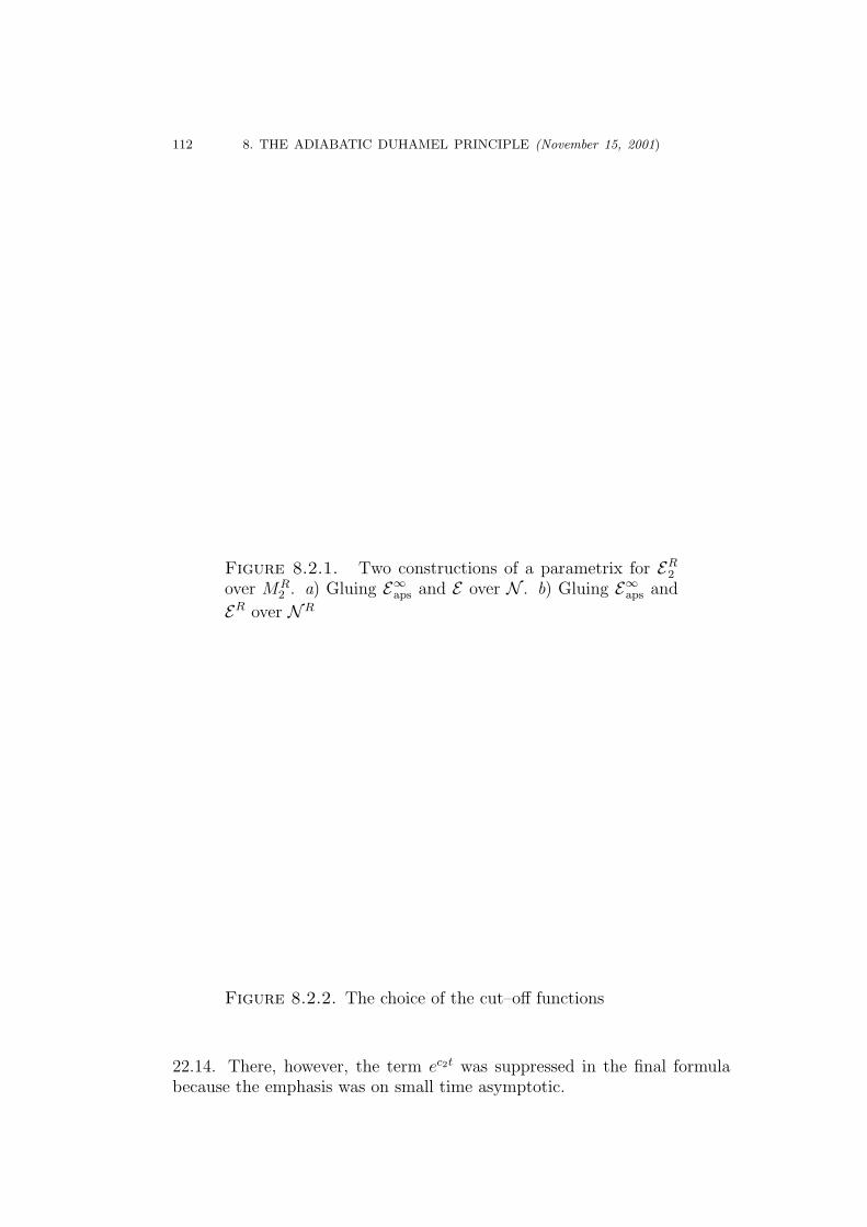
112 8. THE ADIABATIC DUHAMEL PRINCIPLE (November 15, 2001)
Figure 8.2.1. Two constructions of a parametrix for ER2
over MR2 . a) Gluing E∞aps and E over N . b) Gluing E∞aps and
ER over NR
Figure 8.2.2. The choice of the cut–off functions
22.14. There, however, the term ec2t was suppressed in the final formulabecause the emphasis was on small time asymptotic.
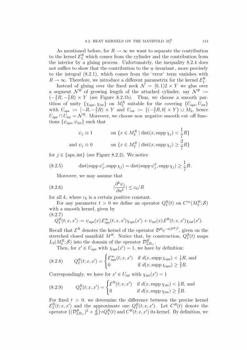
8.2. HEAT KERNELS ON THE MANIFOLD MR2 113
As mentioned before, for R →∞ we want to separate the contributionto the kernel ER
2 which comes from the cylinder and the contribution fromthe interior by a gluing process. Unfortunately, the inequality 8.2.4 doesnot suffice to show that the contribution to the η–invariant , more preciselyto the integral (8.2.1), which comes from the ‘error’ term vanishes withR→∞. Therefore, we introduce a different parametrix for the kernel ER
2 .Instead of gluing over the fixed neck N = [0, 1)2 × Y we glue over
a segment NR of growing length of the attached cylinder, say NR :=(−4
7R,−3
7R) × Y (see Figure 8.2.1b). Thus, we choose a smooth par-
tition of unity {χaps, χint} on MR2 suitable for the covering {Uaps, Uint}
with Uaps := [−R,−37R) × Y and Uint :=
((−4
7R, 0] × Y
)∪ M2, hence
Uaps ∩ Uint = NR. Moreover, we choose non–negative smooth cut–off func-tions {ψaps, ψint} such that
ψj ≡ 1 on {x ∈MR2 | dist(x, suppχj) <
1
7R}
and ψj ≡ 0 on {x ∈MR2 | dist(x, suppχj) ≥
2
7R}
for j ∈ {aps, int} (see Figure 8.2.2). We notice
(8.2.5) dist(suppψ′j, suppχj) = dist(suppψ′′j , suppχj) ≥1
7R .
Moreover, we may assume that
(8.2.6) |∂kψj
∂uk| ≤ c0/R
for all k, where c0 is a certain positive constant.For any parameter t > 0 we define an operator QR
2 (t) on C∞(MR2 ;S)
with a smooth kernel, given by(8.2.7)QR
2 (t;x, x′) := ψaps(x) E∞aps(t;x, x′)χaps(x
′) + ψint(x) ER(t;x, x′)χint(x′).
Recall that ER denotes the kernel of the operator DRe−t(DR)2 , given on thestretched closed manifold MR. Notice that, by construction, QR
2 (t) mapsL2(M
R2 ;S) into the domain of the operator DR
2,Π>.
Then, for x′ ∈ Uaps with χaps(x′) = 1, we have by definition:
(8.2.8) QR2 (t;x, x′) =
{E∞aps(t;x, x
′) if d(x, suppχaps) <17R, and
0 if d(x, suppχaps) ≥ 27R.
Correspondingly, we have for x′ ∈ Uint with χint(x′) = 1
(8.2.9) QR2 (t;x, x′) =
{ER(t;x, x′) if d(x, suppχint) <
17R, and
0 if d(x, suppχint) ≥ 27R.
For fixed t > 0, we determine the difference between the precise kernelER
2 (t;x, x′) and the approximate one QR2 (t;x, x′). Let CR(t) denote the
operator((DR
2,Π>)2 + d
dt
)◦QR
2 (t) and CR(t;x, x′) its kernel. By definition, we
114 8. THE ADIABATIC DUHAMEL PRINCIPLE (November 15, 2001)
have((DR
2,Π>)2 + d
dt
)◦ER
2 (t) = 0. Thus, CR(t) ‘measures’ the error we make
when replacing the precise kernel ER2 (t;x, x′) by the glued, approximate one.
More precisely, we have by Duhamel’s Formula (Proposition 6.3.1)
ER2 (t;x, x′)−QR
2 (t;x, x′) = −∫ t
0
ds
∫MR
2
dz ER2 (s;x, z)CR(t− s; z, x′)
with
CR(t− s; z, x′) =
((DR
2,(z))2 +
d
d(t− s)
)QR
2 (t− s; z, x′)
=
((DR
2 (z))2 − d
ds
)QR
2 (t− s; z, x′)
= ψ′′aps(z) ERaps(t− s; z, x′)χaps(x
′) + 2ψ′aps(z)∂
∂u(ER
aps(t− s; z, x′))χaps(x′)
+ ψaps(z)
(D2
(z) −d
ds
)ER
aps(t− s; z, x′)︸ ︷︷ ︸=0
χaps(x′)
+ ψ′′int(z) ER(t− s; z, x′)χint(x′) + 2ψ′int(z)
∂
∂u(ER(t− s; z, x′))χint(x
′)
+ ψint(z)
((DR
(z))2 − d
ds
)ER(t− s; z, x′)︸ ︷︷ ︸
=0
χint(x′).
Here, D(z) denotes the operator D acting on the z variable; and in the partial
derivative ∂∂u
the letter u denotes the normal coordinate of the variable z.As stated in (8.2.5), the supports of χj and ψ′j (and, equally, ψ′′j ) are
disjoint and separated from each other by a distance R/7 in the normalvariable for j ∈ {aps, int}. Then the error term CR(t − s; z, x′) vanishesboth for the distance in the normal variable d(z, x′) < R/7 and, actually,whenever z or x′ are outside the segment [−6
7R, 1
7R]× Y .
Let z and x′ be on the cylinder and |u− v| > R/7 where u and v denotetheir normal coordinates. We investigate the error term CR(t − s; z, x′)which consists of six summands. Two of them vanish as we have pointed outabove. The remaining four summands involve the kernels E∞aps(t−s; z, x′) on
the infinite cylinder [−R,∞)×Y and ER(t−s; z, x′) on the stretched closedmanifold MR. We shall use that both kernels can be estimated accordingto inequality (8.2.4).
We estimate the first summand
|ψ′′aps(z) E∞aps(t− s; z, x′)χaps(x′)| ≤ c0
Rc1(t− s)−
1+m2 ec2te−c3
d2(z,x′)t−s
≤ c′1ec′2te−c′3R2/t .
Here we have exploited that t ≥ s ≥ 0 and
(t− s)−(1+m)/2e−c2d2(z,x′)(t−s) ≤ ct−(1+m)/2e−c2
d2(z,x′)t ≤ ce−c2
d2(z,x′)2t .
8.2. HEAT KERNELS ON THE MANIFOLD MR2 115
Similarly we estimate the second summand
2|ψ′aps(z)∂
∂uE∞aps(t− s; z, x′)χaps(x
′)|
≤ c0Rc1
(t− s)− 1+m2
√t
ec2te−c3d2(z,x′)
t−s ≤ c′1ec′2te−c′3R2/t ,
where the factor 1/√t comes from the differentiation of the kernel as ex-
plained before.The third and forth summands, involving the kernel ER of the closed
stretched manifold MR, are treated in exactly the same way.Altogether we have proved
Lemma 8.2.2. The error kernel CR(t;u, v) vanishes for u /∈ [−67R,−1
7R].
Moreover, CR(t;u, v) vanishes whenever |u−v| ≤ R/7. For arbitrary x, x′ ∈MR
2 we have the estimate
|CR(t;x, x′)| ≤ c1ec2te−c3R2/t
with constants c1, c2, c3 independent of x, x′, t, R.
We consider the pointwise error
ER2 (t;x, x)−QR
2 (t;x, x) =
∫ t
0
ds
∫MR
2
dz ER2 (s;x, z)CR(t− s; z, x).
We obtain the following proposition as a consequence of the precedinglemma.
Proposition 8.2.3. For all x ∈MR2 and all t > 0 we have
tr ER2 (t;x, x)− trQR
2 (t;x, x) = tr(ER
2 (t;x, x)−QR2 (t;x, x)
).
Moreover, there exist positive constants c1, c2, c3, independent of R, suchthat the ‘error’ term satisfies the inequality
|ER2 (t;x, x)−QR
2 (t;x, x)| ≤ c1 · ec2t · e−c3(R2/t) .
116 8. THE ADIABATIC DUHAMEL PRINCIPLE (November 15, 2001)
Proof. We estimate the error term
|ER2 (t;x, x)−QR
2 (t;x, x)|
≤∫ t
0
ds
∫MR
2
dz |ER2 (s;x, z)CR(t− s; z, x)|
≤ c21ec2t ·
∫ t
0
ds
∫MR
2
dz
{s−
d+12 · e−c3
d2(x,z)s
}· e−c3
d2(x,z)t−s
≤ c21ec2t ·
∫ t
0
ds
∫suppz CR(t−s;z,x)
dz e−c4d2(x,z)
s · e−c3d2(x,z)
t−s
≤ c21ec2t ·
∫ t
0
ds
∫suppz CR(t−s;z,x)
dz e−c5t·R2
s(t−s)
≤ c21ec2t · cR ·
∫ t
0
ds e−c5t·R2
s(t−s) ≤ c21ec2t · 2cR ·
∫ t/2
0
ds e−c5t·R2
s(t/2)
= c21ec2t · 2cR ·
∫ t/2
0
ds e−2c5R2
s .
Here we have used that vol(suppz CR(t− s; z, x)) ∼ vol(Y ) ·R according to
Lemma 8.2.2.We investigate the last integral.∫ t
0
e−cs ds = −
∫ t
0
s2
c· e−
cs · (− c
s2) ds
< −∫ t
0
t2
c· e−
cs · (− c
s2) ds = −t
2
c
∫ ct
∞e−r dr =
t2
ce−
ct .
Thus we have
|ER2 (t;x, x)−QR
2 (t;x, x)| ≤ c21ec2t · 2cR · t2
c6R2e−
c6R2
t ≤ c7ec2t · e−c8(R2/t) .
�
The preceding proposition shows that, for t smaller than√R, the trace
tr ER2 (t;x, x) of the kernel of the operator DR
2 e−t(DR
2,Π>)2 approaches the trace
trQR2 (t;x, x) of the approximative kernel pointwise as R→∞. In particu-
lar, we have:
Corollary 8.2.4. The following equality holds
1√π
∫ √R
0
dt√t
∫MR
2
tr ER2 (t;x, x) dx
=1√π
∫ √R
0
dt√t
∫MR
2
trQR2 (t;x, x) dx+O(e−cR)
as R→∞.
8.2. HEAT KERNELS ON THE MANIFOLD MR2 117
Proof. We have
1√π
∫ √R
0
dt√t
∫MR
2
tr ER2 (t;x, x) dx
=1√π
∫ √R
0
dt√t
∫MR
2
trQR2 (t;x, x) dx
+1√π
∫ √R
0
dt√t
∫MR
2
tr(ER
2 (t;x, x)−QR2 (t;x, x)
)dx,
and we have to show that the second summand on the right side is O(e−cR)as R→∞. We estimate
| 1√π
∫ √R
0
dt√t
∫MR
2
tr(ER
2 (t;x, x)−QR2 (t;x, x)
)dx|
≤ 1√π
∫ √R
0
dt√t
∫MR
2
|ER2 (t;x, x)−QR
2 (t;x, x)| dx
≤ 1√π
∫ √R
0
dt√t
∫MR
2
c1 · ec2t · e−c3(R2/t) dx
≤ c1vol(MR2 )√
π
∫ √R
0
ec2t · e−c3(R2/t)
√t
dt
≤ c4R
∫ √R
0
ec2√
R · e−c5R3/2
dt ≤ c4R3/2 · e−c6R ≤ c7 · e−c8R .
�
Corollary 8.2.4 shows that the essential part of the local η–function ofthe spectral boundary condition on the half manifold with attached cylinderof length R, namely the ‘small–time’ integral from 0 to
√R can be replaced,
as R→∞, by the corresponding integral over the trace trQR2 (t;x, x) of the
approximate kernel, constructed in (8.2.7). Now we show that trQR2 (t;x, x)
can be replaced pointwise (for x ∈ MR2 ) by the trace tr ER(t;x, x) of the
kernel of the operator DRe−t(DR)2 which is defined on the stretched closedmanifold MR.
Consider the Dirac operator
G(∂u +B) : C∞([0,∞)× Y ;S) −→ C∞([0,∞)× Y ;S),
on the half–infinite cylinder with the domain
{s ∈ C∞0 ([0,∞)× Y ;S) | Π>(s|{0}×Y = 0.
It has a unique self–adjoint extension which we denote by Daps. Recall that
the integral kernel E∞aps of the operator Dapse−t(Daps)2 enters in the definition
118 8. THE ADIABATIC DUHAMEL PRINCIPLE (November 15, 2001)
of the approximative kernelQR2 as given in (8.2.7). We show that E∞aps(t;x, x)
is traceless for all x ∈ [0,∞)× Y . Then
(8.2.10) trQR2 (t;x, x) = tr ER(t;x, x) for all x ∈MR
2 ,
follows.To prove that a product TV is traceless, the following quick argument
can be applied occasionally.
Lemma 8.2.5. Let G be unitary with G2 = −Id. We consider an operatorV of trace class which is ‘even’, i.e. it commutes with G. Moreover, T isodd, i.e. it anticommutes with G. Then
Tr(TV ) = 0.
Proof. We have, by unitary equivalence,
Tr(TV ) = Tr(−G(TV )G) = Tr(−GTGV ) = Tr(G2TV ) = Tr(−TV ).
�
Lemma 8.2.6. Let χ : [0,∞) → R be a smooth function with compact
support and t > 0. Then the trace of the operator χ ·Dapse−t(Daps)2 vanishes.
In particular, ∫Y
tr E∞aps(t;u, y;u, y) dy = 0
for all u ∈ [0,∞).
Proof. Clearly, D2aps =
(G(∂u + B)
)2= −∂2
u + B2 is even, hence also
the power series e−t(Daps)2 is even. On the other side, with B also GB isodd. Thus, by Lemmma 9.2.6:
Tr(χ ·GBe−t(Daps)2
)= 0.
To show that
Tr(χ ·G∂ue
−t(Daps)2)
= 0,
we need a slightly more specific argument: Let e∞aps denote the heat kernelof the operator Daps. For u, v ∈ [0,∞) and y, z ∈ Y it has the followingform (see e.g. [27], Formulae 22.33 and 22.35):
eaps(t;u, y; v, z) =∑k∈Z
ek(t;u, v)ϕk(y)⊗ ϕ∗k(z)
for an orthonormal system {ϕk} of eigensections of B. Hence,
G∂u eaps(t;u, y; v, z) =∑k∈Z
e′k(t;u, v)Gϕk(y)⊗ ϕ∗k(z).
8.2. HEAT KERNELS ON THE MANIFOLD MR2 119
But 〈Gϕk;ϕk〉 = 0 on Y since Gϕk is orthogonal to ϕk. �
So far we found
ηDR2,Π>
(0) =1√π
∫ √R
0
dt√t
∫MR
2
tr ER(t;x, x) dx+O(e−cR)
+1√π
∫ ∞
√R
dt√t
∫MR
2
tr ER2 (t;x, x) dx
as R→∞. To prove Theorem 8.1.2, we still have to show
1√π
∫ ∞
√R
dt√t
∫MR
2
tr ER2 (t;x, x) dx = O(e−cR),(8.2.11)
1√π
∫ ∞
√R
dt√t
∫MR
2
tr ER(t;x, x) dx = O(e−cR)(8.2.12)
as R → ∞. Recall that ER2 (t;x, x′) denotes the kernel of the operator
DR2 e
−t(DR2,Π>
)2 on the compact manifold MR2 with boundary {−R}× Y , and
ER(t;x, x′) the kernel of the operator DRe−t(DR)2 on the closed stretchedmanifold MR.
In the following we show (8.2.11), i.e. that we can neglect the contri-bution to the η–invariant of DR
2,Π>which comes from the large time asymp-
totic of ER2 (t;x, x′). The key to that is that the eigenvalue of DR
2,Π>with
the smallest absolute value is uniformly bounded away from zero.
Theorem 8.2.7. Let µ0(R) denote the smallest (in absolute value) non–vanishing eigenvalue of the operator DR
2,Π>on the manifold MR
2 . Let usassume, as always in this chapter, that kerB = {0}. Then there exists apositive constant c0, which does not depend on R such that
µ0(R) > c0
for R sufficiently large.
Remark 8.2.8. The preceding result differs from the behaviour of the smalleigenvalues on the stretched, closed manifold MR. On the manifold withboundary MR
2 with the attached cylinder of length R, the eigenvalues arebounded away from 0 when R→∞ due to the spectral boundary condition.That is the statement of the preceding theorem which we are going to provein the next two sections. On MR, on the contrary, the set of eigenvaluessplits into one set of eigenvalues becoming exponentially small and anotherone of eigenvalues being uniformly bounded away from 0 as R → ∞. Thiswe are going to show further below. Clearly, the reason for the different be-haviour is that on MR
2 the eigensections must satisfy the spectral boundarycondition. Therefore they are exponentially decreasing on the cylinder. But
120 8. THE ADIABATIC DUHAMEL PRINCIPLE (November 15, 2001)
on MR we have to do with eigensections on a closed manifold which neednot decrease, but require part of the eigenvalues to decrease exponentially(for details see Theorem 8.5.1 below).
8.3. Dirac Operators on Manifolds with Cylindrical Ends
To prove Theorem 8.2.7 we first recall a few properties of the cylin-drical Dirac operator Dcyl := G(∂u + B) on the infinite cylinder Y ∞
cyl :=(−∞,+∞) × Y . A special feature of the cylindrical manifold Y ∞
cyl is thatwe may apply the theory of Sobolev spaces exactly as in the case of Rm.The point is that we can choose a covering of the open manifold Y ∞
cyl bya finite number of coordinate charts. We can also choose a finite trivial-ization of the bundle S|Y∞cyl
. Let {Uι, κι}Kι=1 be such a trivialization, where
κι : S|Uι → Vι×CN is a bundle isomorphism and Vι an open (possibly non–compact) subset of Rm. Let {fι} be a corresponding partition of unity. Weassume that for any ι the derivatives of the function fι are bounded.
Definition 8.3.1. We say that a section (or distribution) s of the bundleS over Y ∞
cyl belongs to the p-th Sobolev space Hp(Y ∞cyl ;S), p ∈ R, if and only
if fι · s belongs to the Sobolev space Hp(Rm; CN) for any ι. We define thep-th Sobolev norm
‖s‖p :=K∑
ι=1
‖(Id + ∆ι)p/2(fι · s)‖L2(Rm) ,
where ∆ι denotes the Laplacian on the trivial bundle Vι×CN ⊂ Rm×CN .
Lemma 8.3.2. (a) For the unique self–adjoint L2–extension of Dcyl (denotedby the same symbol) we have
dom(Dcyl) = H1(Y ∞cyl ;S).
(b) Let λ1 denote the smallest positive eigenvalue of the operator B on themanifold Y . Then we have
(8.3.1) 〈(Dcyl)2s; s〉 ≥ λ2
1‖s‖2
for all s ∈ dom(Dcyl), and for any µ ∈ (−λ1,+λ1) the operator
Dcyl − µ : H1(Y ∞cyl ;S) −→ L2(Y
∞cyl ;S)
is an isomorphism of Hilbert spaces.(c) Let Rcyl(µ) denote the inverse of the operator Dcyl−µ. Then the family{Rcyl(µ)}µ∈(−λ1,λ1) is a smooth family of elliptic pseudo–differential opera-tors of order −1.
8.3. DIRAC OPERATORS ON MANIFOLDS WITH CYLINDRICAL ENDS 121
Proof. (a) follows immediately from the corresponding result on themodel manifold Rm.To prove (b) we consider a spectral resolution {ϕk, λk}k∈Z\0 of L2(Y ;S)generated by the tangential operator B. Because of (8.1.2) we have λ−k =−λk. We consider a section s belonging to the dense subspace C∞
0 (Y ∞cyl ;S)
of dom(Dcyl), and expand it in terms of the preceding spectral resolution
s(u, y) =∑
k∈Z\{0}
fk(u)ϕk(y).
Since (Dcyl)2 = −∂2
u +B2, we obtain
(Dcyl)2s =
∑(λ2
kfk − f ′′k )ϕk,
hence
〈(Dcyl)2s; s〉 =
∑∫ ∞
−∞(λ2
kfk(u)− f ′′k (u))fk(u)du
≥ λ21‖s‖2 −
∑∫ ∞
−∞f ′′k (u)fk(u)du
= λ21‖s‖2 +
∑∫ ∞
−∞f ′k(u)f ′k(u)du ≥ λ2
1‖s‖2 .
It follows that (Dcyl)2 (and therefore Dcyl) has bounded inverse in L2(Y
∞cyl ;S)
and, more generally, that (Dcyl)2 − µ is invertible for µ ∈ (−λ1, λ1).
To prove (c) we apply the symbolic calculus and construct a parametrix Sfor the operator Dcyl, i.e. S is an elliptic pseudo–differential operator oforder −1 such that
SDcyl = Id + T,
where T is a smoothing operator. Thus
D−1cyl = S − TD−1
cyl .
The operator TD−1cyl is a smoothing operator, henceD−1
cyl is an elliptic pseudo–differential operator of order −1. The same argument can be applied to theresolvent Rcyl(µ) = (Dcyl − µ)−1 for arbitrary µ ∈ (−λ1, λ1). The smooth-ness of the family follows by standard calculation. �
To prove Theorem 8.2.7 we need to refine the preceding results on theinfinite cylinder Y ∞
cyl to the Dirac operator, naturally extended to the ma-
nifold M∞2 =
((−∞, 0] × Y
)∪M2 with cylindrical end. Let C∞
0 (M∞2 ,S)
denote the space of compactly supported smooth sections of S over M2.Then
(8.3.2) D∞2 |C∞0 (M∞2 ,S) : C∞
0 (M∞2 ,S)→ L2(M
∞2 ,S)
is symmetric. Moreover, we have
122 8. THE ADIABATIC DUHAMEL PRINCIPLE (November 15, 2001)
Lemma 8.3.3. Let s ∈ C∞(M∞2 ;S) be an eigensection of D∞2 . Then there
exist C, c > 0 such that, on (−∞, 0]× Y , we have |s(u, y)| ≤ Cecu.
Proof. Let {ϕk, λk}k∈Z\0 be a spectral resolution of the tangential op-erator B. Because of (8.1.2) we have λ−k = −λk and we can assume thatϕ−k = Gϕk for k ∈ N. Then
(8.3.3)
{ϕ±k =
1√2
(ϕk ±Gϕk
),±λk
}k∈N
is a spectral resolution of the composed operator GB on Y . Notice that wehave
(8.3.4) Gϕ+k = −ϕ−k and Gϕ−k = ϕ+
k .
Let s ∈ C∞(M∞2 ;S) and
(8.3.5) D∞L2ψ = µψ
with µ ∈ R. We expand s|(−∞,0]×Y in terms of the spectral resolution ofGB just constructed:
s(u, y) =∞∑
k=1
fk(u)ϕ+k (y) + gk(u)ϕ−k .
Because of (8.3.3), (8.3.4), and (8.3.5) the coefficients fk, gk must satisfythe system of ordinary differential equations(
λk ∂/∂u−∂/∂u −λk
)(fk
gk
)= µ
(fk
gk
)or, equivalently,(
f ′kg′k
)= A
(fk
gk
)with A :=
(0 −(µ+ λk)
µ− λk 0
).
Since s ∈ L2, of the eigenvalues ±√λ2
k − µ2 of A only those which are onthe positive real line enter in the construction of s by solving the preced-ing differential equation. In particular, all coefficients fk, gk must vanishidentically for λk ≤ µ. Thus
(8.3.6) s(u, y) =∑λk>µ
ak
(exp(√
λ2k − µ2 u
)ϕ+
k
− λk − µ√λ2
k − µ2exp(√
λ2k − µ2 u
)ϕ−k
),
and, in particular,
|s(u, y)| ≤ C exp(√
λ2k0− µ2
u
2
), u < 0,
for some constant C when λk0 denotes the smallest positive eigenvalue of Bsuch that λk0 > |µ|. �
8.3. DIRAC OPERATORS ON MANIFOLDS WITH CYLINDRICAL ENDS 123
In spectral theory we are looking for self–adjoint L2–extensions of asymmetric operator. We recall: on a closed manifold, the Dirac operatoris essentially self–adjoint; i.e. its minimal closed extension is self–adjoint(and therefore there do not exist other self–adjoint extensions) and it is aFredholm operator. On a compact manifold with boundary, the situation ismuch more complicated. There is a huge variety of dense domains to whichthe Dirac operator can be extended such that it becomes self–adjoint; andthere is a smaller, but still large variety where the extension of the Diracoperator becomes self–adjoint and Fredholm (see e.g. Booß-Bavnbek andFurutani [20]); a special type of self–adjoint and Fredholm domains arethe domains specified by the boundary conditions belonging to the Grass-mannian of all self–adjoint generalized Atiyah–Patodi–Singer projections.These boundary conditions are treated in this book.
Now we shall show that the situation on manifolds with (infinite) cylin-drical ends resembles the situation on closed manifolds.
We recall the following simple lemma (see also Reed and Simon [85],Theorem VIII.3, Corollary, p. 257).
Lemma 8.3.4. Let A be a densely defined symmetric operator in a separablecomplex Hilbert space H. We assume that range(A+ i) is dense in H. ThenA is essentially self–adjoint.
Proof. Since A is symmetric, the operator A + i is injective and theoperator (A + i)−1 is well defined and bounded on the dense subspacerange(A + i) of H. Then the closure Ri of (A + i)−1 has the whole spaceH as domain and Ri is bounded and injective. Now a standard argumentof functional analysis (see e.g. Pedersen [80], Proposition 5.1.7) says thatthe inverse R−1
i of a densely defined, closed, and injective operator Ri hasthe same properties. Thus our R−1
i is closed; and by construction it is theminimal closed extension of A+ i. Therefore, R−1
i − i is symmetric and theminimal closed extension of A, hence self–adjoint and equal A∗. �
We apply the lemma for H = L2(M∞2 ;S) and take for A the operator
of (8.3.2). To prove that the range (D∞2 + i)(C∞0 (M∞
2 ;S)) is dense inL2(M
∞2 ;S) we consider a section s ∈ L2(M
∞2 ;S) which is orthogonal to
(D∞2 +i)(C∞0 (M∞
2 ;S)); i.e. the distribution (D∞2 −i)s vanishes when appliedto any test function, hence
(8.3.7) (D∞2 − i)s = 0.
Since D∞2 − i is elliptic, by elliptic regularity s is smooth in all inner points,that is for our complete manifold in all points. On the cylinder (−∞, 0]×Ywe expand s in terms of the eigensections of the composed operator GB onY . It follows that s satisfies an estimate of the form
(8.3.8) |s(u, y)| ≤ Cecu, (u, y) ∈ (−∞, 0]× Y,
124 8. THE ADIABATIC DUHAMEL PRINCIPLE (November 15, 2001)
for some constants C, c > 0 (according to Lemma 8.3.3). On the manifoldMR
2 with cylindrical end of finite length R we apply Green’s formula andget
(8.3.9) 〈DR2 s
R; sR〉 − 〈sR;DR2 s
R〉 = −∫{−R}×Y
(Gs|{−R}×Y dy, s|{−R}×Y ),
where sR denotes the restriction of s to the manifold MR2 with boundary
{−R}× Y . For R→∞, the right side of (8.3.9) vanishes; and the left sidebecomes 2i‖s‖2 by (8.3.7). Hence s = 0.
Thus we have proved
Lemma 8.3.5. The operator (8.3.2) is essentially self–adjoint.
We denote the (unique) self–adjoint L2–extension by the same symbolD∞2 .
We define the Sobolev spaces on the manifold M∞2 like in Definition
8.3.1. Once again, the point is that manifolds with cylindrical ends, eventhey are not compact but only complete, are like the infinite cylinder suffi-cient simple to be covered by a finite system of local charts. Clearly
dom(D∞2 ) = H1(M∞2 ;S)
and
D∞2 : H1(M∞2 ;S)→ L2(M
∞2 ;S)
is bounded. There are, however, substantial differences between the proper-ties of the simple Dirac operator Dcyl on the infinite cylinder and the Diracoperator D∞2 on the manifold with cylindrical end. For instance, from Bthe discreteness of the spectrum and the regularity at 0 (i.e., 0 is not aneigenvalue) are passed on to Dcyl, but not to D∞2 . Yet we can prove thefollowing result:
Proposition 8.3.6. The operator
D∞2 : dom(D∞2 ) = H1(M∞2 ;S) −→ L2(M
∞2 ;S)
is a Fredholm operator and its spectrum in the interval (−λ1, λ1) consists offinitely many eigenvalues of finite multiplicity. Here λ1 denotes the smallestpositive eigenvalue of B.
Note . The first part of the proposition is false, if we drop the assump-tion of invertible tangential operator B, see Example ?? below. The secondpart of the proposition remains true also for singular B. Actually, usingmore advanced methods one can show that the essential spectrum of D∞2 isequal to (−∞,−λ1] ∪ [λ1,∞) (see for instance Muller [73], Section 4).
8.3. DIRAC OPERATORS ON MANIFOLDS WITH CYLINDRICAL ENDS 125
Before proving the proposition we shall collect various criteria for thecompactness of a bounded operator between Sobolev spaces on an openmanifold. Let X be a complete (not necessarily compact) Riemannian ma-nifold with a fixed Hermitian bundle. Recall the three cornerstones of theSobolev analysis of Dirac operators for X closed.
Rellich Lemma: The inclusion H1(X) ↪→ L2(X) is compact.Compact Resolvent: To each Dirac operatorD we have a parametrixR which is an elliptic pseudo–differential operator of order −1 withprincipal symbol equal to the inverse of the principal symbol of D.So it is a bounded operator from L2(X) to H1(X), hence compactin L2(X). In particular, for µ in the resolvent set the resolvent(D − µ)−1 is compact as operator in L2(X).
Smoothing Operator: Any integral operator over X with smoothkernel is a smoothing operator, i.e. it maps distributional sectionsof arbitrary low order into smooth sections. Moreover, it is of traceclass and thus compact.
In the general case, i.e. for not necessarily compact X, the RellichLemma remains valid for sections with compact support. A compact re-solvent is not attainable, hence the essential spectrum appears. Operatorswith smooth kernel remain smoothing operators, but in general they are nolonger of trace class nor compact. We recall:
Lemma 8.3.7. Let X be a complete (not necessarily compact) Riemannianmanifold with fixed Hermitian bundle. Let K be a compact subset of X.(a) The injection H1(X) ↪→ L2(X) defines a compact operator when werestrict it to all sections with support in K. In particular, for any cut–off function χ with support in K and any bounded operator R : L2(X) →H1(X) the operator χR is compact in L2(X).(b) Let T : L2(X)→ L2(X) be an integral operator with a kernel k(x, y) ∈L2(X
2). Then the operator T is a bounded, compact operator (in fact it isof Hilbert–Schmidt class).(c) Let T : L2(X)→ L2(X) be a bounded compact operator and H′ a closedsubspace of L2(X), e.g. H′ := L2(X
′) where X ′ is a submanifold of X ofcodimension 0. Assume that T (H′) ⊂ H′. Then T |H′ is compact as operatorfrom H′ to H′.
Proof. (a) follows immediately from the local Rellich Lemma. (b)is the famous Hilbert–Schmidt Lemma. Also (c) is well known, see e.g.Hormander [54], Proposition 19.1.13 where (c) is proved within the categoryof trace class operators. �
In general an integral operator T with smooth kernel is not compacteven if either suppx k(x, x′) or suppx′ k(x, x′) are contained in a compactsubset K ⊂ X. Consider for instance on Y ∞
cyl = (−∞,+∞)× Y an integral
126 8. THE ADIABATIC DUHAMEL PRINCIPLE (November 15, 2001)
operator T with a smooth kernel of the form
k(x, x′) = χ(x)d(x, x′),
where d(x, x′) denotes the distance and χ is a function with support in aball of radius 1 (and equal 1 in a smaller ball). Then T is not a compactoperator on L2(Y
∞cyl): choose a sequence {sn} of L2 functions of norm 1 and
with supp sn contained in a ball of radius 1 such that d(suppχ, supp sn) = n.Then for any n we have ‖Tsn‖ > Cn. Thus T is not compact, in fact noteven bounded.
For the bounded resolvent (see Lemma 8.3.2)
Rcyl : L2(Y∞cyl ;S)→ H1(Y ∞
cyl ;S)
we have, however, the following corollary to the preceding lemma. It pro-vides an example of a compact integral operator on an open manifold witha smooth kernel which is compactly supported only in one variable.
Corollary 8.3.8. Let χ and ψ be smooth cut–off functions on Y ∞cyl with
support contained in the half–cylinder (−∞, 0)×Y . Let suppχ be compact.Then the operators χRcylψ and ψRcylχ are compact in L2(Y
∞cyl ;S).
Proof. The operator χRcylψ is compact according to the precedinglemma, claim (a). Its adjoint operator is ψRcylχ, since Rcyl is self–adjoint.Thus it is also compact (even if its range is not compactly supported). �
Proof of the Proposition. Let µ ∈ (−λ1, λ1). We show that theoperator D∞2 − µ is an (unbounded) Fredholm operator in L2(M
∞2 ;S). To
do that we construct a parametrix R∞2 (µ) for D∞2 − µ. Let Rcyl(µ) denotethe inverse operator of Dcyl − µ on the infinite cylinder Y ∞
cyl introduced inLemma 8.3.2. Let R(µ) be a parametrix for the operator D − µ on theclosed partitioned manifold M . We may assume that R(µ) is an ellipticpseudo–differential operators of order −1 such that
R(µ)(D − µ
)= Id− T (µ) and
(D − µ
)R(µ) = Id− T ′(µ),
where T (µ), T ′(µ) are operators with smooth kernels, hence compact andeven of trace class because they are on a closed manifold. Moreover, wemay assume that the operator family {R(µ)} is a smooth family.
We glue the two parametrices Rcyl(µ) and R(µ) over a narrow segmentof the neck, say N 1 = (−4
7,−3
7) × Y (see Figure 8.3.1) in a similar way
as we have done before for the heat kernels. Thus, we choose a smoothpartition of unity {χcyl, χint} on M∞
2 suitable for the covering {Ucyl, Uint}with Ucyl := (−∞,−3
7)×Y and Uint := (−4
7, 0]×Y ∪M2, hence Ucyl∩Uint =
N 1. Moreover, we choose non–negative smooth cut–off functions {ψcyl, ψint}
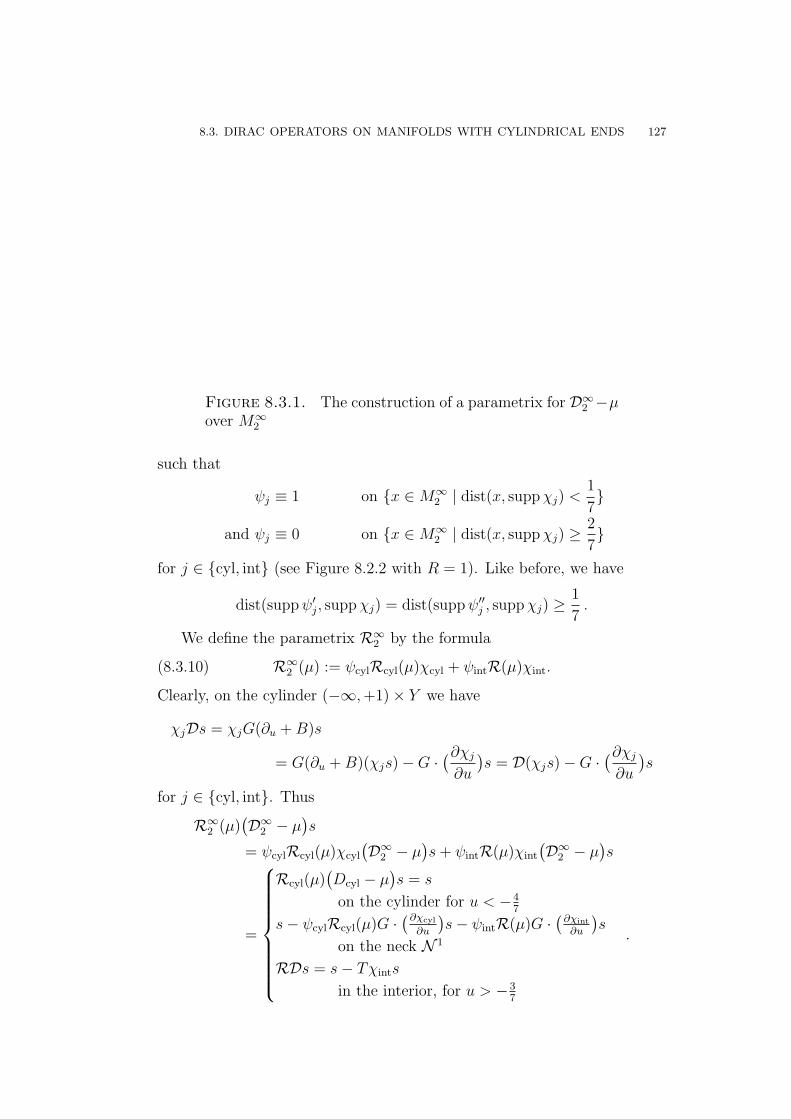
8.3. DIRAC OPERATORS ON MANIFOLDS WITH CYLINDRICAL ENDS 127
Figure 8.3.1. The construction of a parametrix for D∞2 −µover M∞
2
such that
ψj ≡ 1 on {x ∈M∞2 | dist(x, suppχj) <
1
7}
and ψj ≡ 0 on {x ∈M∞2 | dist(x, suppχj) ≥
2
7}
for j ∈ {cyl, int} (see Figure 8.2.2 with R = 1). Like before, we have
dist(suppψ′j, suppχj) = dist(suppψ′′j , suppχj) ≥1
7.
We define the parametrix R∞2 by the formula
(8.3.10) R∞2 (µ) := ψcylRcyl(µ)χcyl + ψintR(µ)χint.
Clearly, on the cylinder (−∞,+1)× Y we have
χjDs = χjG(∂u +B)s
= G(∂u +B)(χjs)−G ·(∂χj
∂u
)s = D(χjs)−G ·
(∂χj
∂u
)s
for j ∈ {cyl, int}. Thus
R∞2 (µ)(D∞2 − µ
)s
= ψcylRcyl(µ)χcyl
(D∞2 − µ
)s+ ψintR(µ)χint
(D∞2 − µ
)s
=
Rcyl(µ)(Dcyl − µ
)s = s
on the cylinder for u < −47
s− ψcylRcyl(µ)G ·(∂χcyl
∂u
)s− ψintR(µ)G ·
(∂χint
∂u
)s
on the neck N 1
RDs = s− Tχints
in the interior, for u > −37
.
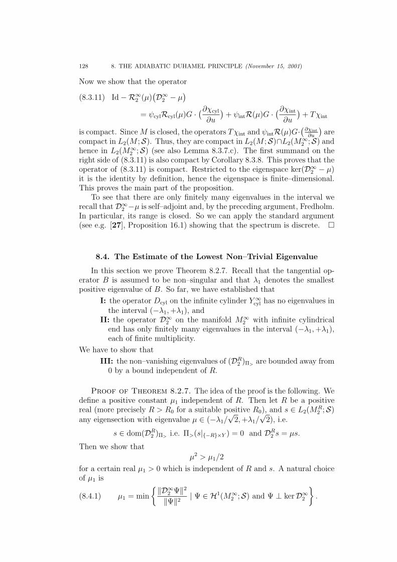
128 8. THE ADIABATIC DUHAMEL PRINCIPLE (November 15, 2001)
Now we show that the operator
(8.3.11) Id−R∞2 (µ)(D∞2 − µ
)= ψcylRcyl(µ)G ·
(∂χcyl
∂u
)+ ψintR(µ)G ·
(∂χint
∂u
)+ Tχint
is compact. Since M is closed, the operators Tχint and ψintR(µ)G·(
∂χint
∂u
)are
compact in L2(M ;S). Thus, they are compact in L2(M ;S)∩L2(M∞2 ;S) and
hence in L2(M∞2 ;S) (see also Lemma 8.3.7.c). The first summand on the
right side of (8.3.11) is also compact by Corollary 8.3.8. This proves that theoperator of (8.3.11) is compact. Restricted to the eigenspace ker(D∞2 − µ)it is the identity by definition, hence the eigenspace is finite–dimensional.This proves the main part of the proposition.
To see that there are only finitely many eigenvalues in the interval werecall that D∞2 −µ is self–adjoint and, by the preceding argument, Fredholm.In particular, its range is closed. So we can apply the standard argument(see e.g. [27], Proposition 16.1) showing that the spectrum is discrete. �
8.4. The Estimate of the Lowest Non–Trivial Eigenvalue
In this section we prove Theorem 8.2.7. Recall that the tangential op-erator B is assumed to be non–singular and that λ1 denotes the smallestpositive eigenvalue of B. So far, we have established that
I: the operator Dcyl on the infinite cylinder Y ∞cyl has no eigenvalues in
the interval (−λ1,+λ1), andII: the operator D∞2 on the manifold M∞
2 with infinite cylindricalend has only finitely many eigenvalues in the interval (−λ1,+λ1),each of finite multiplicity.
We have to show that
III: the non–vanishing eigenvalues of (DR2 )Π> are bounded away from
0 by a bound independent of R.
Proof of Theorem 8.2.7. The idea of the proof is the following. Wedefine a positive constant µ1 independent of R. Then let R be a positivereal (more precisely R > R0 for a suitable positive R0), and s ∈ L2(M
R2 ;S)
any eigensection with eigenvalue µ ∈ (−λ1/√
2,+λ1/√
2), i.e.
s ∈ dom(DR2 )Π> i.e. Π>(s|{−R}×Y ) = 0 and DR
2 s = µs.
Then we show that
µ2 > µ1/2
for a certain real µ1 > 0 which is independent of R and s. A natural choiceof µ1 is
(8.4.1) µ1 = min
{‖D∞2 Ψ‖2
‖Ψ‖2| Ψ ∈ H1(M∞
2 ;S) and Ψ ⊥ kerD∞2}.
8.4. THE ESTIMATE OF THE LOWEST NON–TRIVIAL EIGENVALUE 129
Figure 8.4.1. a) Continuous extension of a given eigensec-tion by a nullsection. b) With growing R the enlargement αand the cosine β decrease exponentially and the norm of theprojection s goes to 1
Note that by II above (Proposition 8.3.6) the nullspace kerD∞2 is of finitedimension. We shall define a certain extension s∞ ∈ H1(M∞
2 ;S) of s.Quite a comfortable reasoning would be achieved, if we could extend s
to an eigensection of D∞2 on all of M∞2 . Then it follows at once that the
discrete part of the spectrum of D∞2 is not empty, µ belongs to it,√µ1 is
the smallest eigenvalue > 0, and hence we have µ2 > µ1/2 as wanted.In general, such a convenient extension of the given eigensection s can
not be achieved. But due to the spectral boundary condition satisfied by s inthe hypersurface {−R}×Y , the eigensection s over MR
2 can be continuouslyextended by a section over (−∞,−R] × Y on which the Dirac operatorvanishes (see Figure 8.4.1a). By construction, both the enlargement α ofthe L2 norm of s by the chosen extension and the cosine β of the anglebetween s∞ and kerD∞2 can be estimated independently of the specificchoice of s and µ. It turns out that they both decrease exponentially withgrowing R (see Figure 8.4.1b).
130 8. THE ADIABATIC DUHAMEL PRINCIPLE (November 15, 2001)
Let {s1, . . . , sq} be an orthonormal basis of kerD∞2 and set
s := s∞ −q∑
j=1
〈s∞; sj〉sj .
Clearly, the section s belongs to H1(M∞2 ;S) and is orthogonal to kerD∞2 .
Hence, on one side,
(8.4.2)‖D∞2 s‖2
‖s‖2≥ µ1 .
On the other side, we have by construction
‖D∞2 s‖2 = ‖D∞2 s∞‖2 = ‖DR2 s‖2MR
2= µ2 .
Finally, we shall prove that
(8.4.3) ‖s‖ → 1 as R→∞.
Then the estimate
(8.4.4) µ2 >µ1
2
follows for sufficiently large R. Since we have assumed that µ2 <λ21
2, we
have also µ1 < λ21, hence µ1 belongs to the discrete part of the spectrum of
(D∞2 )2 and, by the Min–Max Principle (see, for instance, [87]), must be itssmallest eigenvalue > 0.
Thus, to prove the theorem we are left with the task of first constructinga suitable extension s of s and then proving (8.4.3).
We expand s|[−R,0]×Y in terms of a spectral resolution
{ϕk, λk;Gϕk,−λk}k∈N
of L2(Y ;S) generated by B:
s(u, y) =∞∑
k=1
fk(u)ϕk(y) + gk(u)Gϕk .
Since G(∂u + B)s|[−R,0]×Y = 0, the coefficients must satisfy the system ofordinary differential equations
(8.4.5)
(f ′kg′k
)= Ak
(fk
gk
)with Ak :=
(−λk µ−µ λk
).
Moreover, since Π>s|{−R}×Y = 0 we have
(8.4.6) fk(−R) = 0 for any k ≥ 1.
Thus, for each k the pair (fk, gk) is uniquely determined up to a constantak. More explicitly, since the eigenvalues of Ak are ±(λ2
k−µ2)1/2, a suitable
8.4. THE ESTIMATE OF THE LOWEST NON–TRIVIAL EIGENVALUE 131
choice of the eigenvectors of Ak gives
fk(u) = akµ√
λ2k − µ2
sinh√λ2
k − µ2(R + u) and
gk(u) = ak
(cosh
√λ2
k − µ2(R + u) +λk√λ2
k − µ2sinh(λ2
k − µ2)1/2(R + u)).
We assume ‖s‖L2 = 1. Then we have, with v := (λ2k − µ2)1/2(R + u):
1 ≥∫
[−R,0]×Y
|s(u, y)|2 dudy =∞∑
k=1
∫ 0
−R
(|fk(u)|2 + |gk|2
)du
=∞∑
k=1
|ak|21
(λ2k − µ2)1/2
∫ (λ2k−µ2)1/2R
0
( µ2
λ2k − µ2
· sinh2 v
+ cosh2 v + 2λk
(λ2k − µ2)1/2
· cosh v · sinh v +λ2
k
λ2k − µ2
· sinh2 v)dv
=∞∑
k=1
|ak|2{− λ2
k
λ2k − µ2
·R + (1/4) · µ2
(λ2k − µ)3/2
· sinh(2(λ2k − µ2)1/2R)
+ (1/4) ·(
1 +λ2
k
λ2k − µ2
)· (λ2
k − µ2)1/2 · sinh(2(λ2k − µ2)1/2R)
+λ2
k
λ2k − µ2
· cosh2((λ2k − µ2)1/2R)
}.
Since λ2k ≥ λ2
1 > 2µ2 we have 2(λ2k − µ2)1/2 >
√2λk > λk. Moreover, we
have for all k ≥ 1
− λ2k
λ2k − µ2
·R +λ2
k
λ2k − µ2
· (λ2k − µ2)1/2
4· sinh(2(λ2
k − µ2)1/2R)
> −R +(λ2
1 − µ2)1/2
4· sinh(2(λ2
1 − µ2)1/2R)
> −R +
√2
8λ1 · sinh(
√2λ1R) > 0,
if R ≥ R0 for some positive R0 which depends only on λ1 and not on µ noron s nor on k.
Thus, for any k the sum in the braces can be estimated in the followingway:{
. . .}>
λ2k
λ2k − µ2
· cosh2((λ2k − µ2)1/2R) >
1
4e2(λ
2k−µ2)1/2R >
1
4eλkR .
Hence, we have
(8.4.7)∞∑
k=1
|ak|2 · eλkR ≤ 4 .
132 8. THE ADIABATIC DUHAMEL PRINCIPLE (November 15, 2001)
Note that the preceding estimate does not depend on R (provided thatR > R0) nor on k nor on the specific choice of s, and that R0 only dependson λ1.
According to (8.4.7) the absolute value of the coefficients ak is rapidlydecreasing in such a way that, in particular, we can extend the eigensections of DR
2,Π>, given on MR
2 to a continuous section on M∞2 by the formula
s∞(x) :=
{s(x) for x ∈MR
2∑∞k=1 ake
λk(R+u)Gϕk(y) for x = (u, y) ∈ (−∞,−r]× Y .
By construction, s∞ is smooth on M∞2 \ ({−R} × Y ) and belongs to the
Sobolev space H1(M∞2 ;S). It follows from (8.4.7) that
‖s∞‖2L2= ‖s‖2L2
+∞∑
k=1
|ak|2∫ −R
−∞e2λk(R+u) du = 1 +
∞∑k=1
|ak|21
2λk
≤ 1 +1
2λ1
·∞∑
k=1
|ak|2 ≤ 1 +1
2λ1
·( ∞∑
k=1
|ak|2 · eλkR)· e−λ1R
≤ 1 +2
λ1
· e−λ1R .(8.4.8)
Next, let Ψ ∈ kerD∞2 and assume that ‖Ψ‖ = 1. By (8.3.6), the sectionΨ has on (−∞, 0]× Y the form
(8.4.9) Ψ((u, y) =∞∑
k=1
bkeλkuG(y)ϕk(y)
with ∑∫ 0
−∞|bk|2e2λku du =
∑ 1
2λk
· |bk|2 < +∞.
Set l := Ψ|MR2
. Then l satisfies the equations
DR2 l = 0 and Π>(l|{−R}×Y ) = 0.
Hence, l belongs to kerDR2,Π>
. This implies the following equality:∫MR
2
〈s∞(x); Ψ(x)〉dx =1
µ·∫
MR2
〈DR2 s
∞(x); l(x)〉dx
=1
µ·∫
MR2
〈s∞(x);DR2 l(x)〉dx− 1
µ·∫
Y
〈Gs∞(−R, y); l(−R, y)〉dx.
On the other hand,∫(−∞,−r]×Y
〈s∞(x); Ψ(x)〉dx =∑k>0
akbk2µ· e−λkR ≤ C1e−λ1R .
Therefore
(8.4.10) |〈s∞; Ψ〉| ≤ C1e−λ1R .
Hence, we have proved
8.4. THE ESTIMATE OF THE LOWEST NON–TRIVIAL EIGENVALUE 133
Lemma 8.4.1. Any eigensection s ∈ H1(MR2 ;S) of DR
2,Π>with eigenvalue
µ ∈ (−λ1/√
2, λ1/√
2) can be extended to a continuous section s∞ on M∞2
which is smooth on M∞2 \ ({−R} × Y ) and belongs to the first Sobolev space
H1(M∞2 ;S). Moreover, the enlargement of the norm of s by the extension
and the cosine of the angle between s∞ and kerD∞2 are exponentially de-creasing by formulae (8.4.8) and (8.4.10).
The final step in proving the theorem follows at once from the precedinglemma. We recall: by definition of µ1 we have ‖D∞2 s‖2/‖s‖2 ≥ µ1 and byconstruction of s we have ‖D∞2 s‖2 = µ2. Thus, we have µ2 ≥ ‖s‖2 · µ1. Toestablish the wanted bound µ2 > µ1/2, it remains to show that ‖s‖2 > 1/2for sufficiently large R.
Since s is the orthogonal projection of s∞ onto (kerD∞2 )⊥ and by theorthonormality of the basis {s1, . . . , sq} of kerD∞2 , we have
‖s‖2 = ‖s∞‖2 −q∑
j=1
|〈s∞; sj〉|2 ≤ 1 +2
λ1
e−λ1R −q∑
j=1
|〈s∞; sj〉|2 .
Thus,
|‖s‖2 − 1| ≤ 2
λ1
e−λ1R + qC1e−2λ1R ≤ C2e
−C3R ,
which proves the theorem. �
We finish this section by proving the asymptotic estimate (8.2.11). Re-
call that ER2 (t;x, x′) denotes the kernel of the operator DR
2,Π>e−t(DR
2,Π>)2
where DR2,Π>
denotes the Dirac operator over the manifold MR2 with the
spectral boundary condition at the boundary {−R} × Y . Then we have:
Lemma 8.4.2.
1√π
∫ ∞
√R
dt√t
∫MR
2
tr ER2 (t;x, x) dx = O(e−cR).
Proof. For any eigenvalue µ 6= 0 of DR2,Π>
and R > 0 sufficiently large
(R · c20 ≥ 1, where c0 denotes the lower uniform bound for µ2 of Theorem8.2.7) we have
(8.4.11) |∫ ∞
√R
1√tµe−tµ2
dt| ≤∫ ∞
√R
1√t|µ|e−tµ2
dt =
∫ ∞
|µ|R1/4
e−τ2
dτ
≤∫ ∞
|µ|R1/4
τe−τ2
dτ =
[−1
2e−τ2
]∞|µ|R1/4
1
2e−µ2
√R ,
134 8. THE ADIABATIC DUHAMEL PRINCIPLE (November 15, 2001)
which gives
|∫ ∞
√R
dt√t
∫MR
2
Tr(DR
2,Π>e−t(DR
2,Π>)2)| ≤
∫ ∞
√R
dt√t
∫MR
2
∑µ 6=0
|µ|e−tµ2
dt
≤ 1
2·∑µ 6=0
e−µ2√
R =1
2·∑µ 6=0
e−(√
R−1)µ2 · e−µ2
≤ C1 · e−√
Rµ20 Tr(e−
(DR
2,Π>
)2)≤ C2 · e−
√Rµ2
0vol(MR2 )
≤ C3 · e−√
Rµ20 ≤ C3 · e−C4
√R .
Here we have exploited that the heat kernel eR2 (t;x, x′) of the operator DR
2,Π>
can be estimated by
|eR2 (t;x, x′)| ≤ c1 · t−
m2 · ec2t · e−c3
d2(x,x′)t
according to (8.2.3). Thus,
(8.4.12) |Tr(e−
(DR
2,Π>
)2)| ≤
∫MR
2
|tr eR2 (1; x, x)| dx ≤ c1 · ec2 ·
∫MR
2
dx.
�
8.5. The Spectrum on the Closed Stretched Manifold
So far we proved the asymptotic equation
1√π
∫ √R
0
dt√t
∫MR
2
tr ER(t;x, x) dx+O(e−cR) = ηDR2,Π>
(0)
as R→∞. It follows that
limR→∞
ηR = limR→∞
(ηDR
1,Π<(0) + ηDR
2,Π>(0)),
where
ηR :=1√π
∫ √R
0
dt√t
∫MR
tr ER(t;x, x) dx.
To prove Theorem 8.1.2, we still have to show (8.2.12), i.e., that we can
extend the integration from√R to infinity:
1√π
∫ ∞
√R
dt√t
∫MR
2
tr ER(t;x, x) dx = O(e−cR) as R→∞.
Recall that ER(t;x, x′) denotes the kernel of the operator DRe−t(DR)2 on theclosed stretched manifold MR.
Formally, our task of proving the preceding estimate reminds of our pre-vious task of proving the corresponding estimate for the kernel ER
2 (t;x, x′)
of the operator DR2 e
−t(DR2,Π>
)2 (see Lemma 8.4.2). Both integrals are overthe same prolonged compact manifold MR
2 with boundary {−R} × Y . Themethods we can apply are, however, different: In the previous case, we had a
8.5. THE SPECTRUM ON THE CLOSED STRETCHED MANIFOLD 135
uniform positive bound for the absolute value of the smallest non–vanishingeigenvalue of the boundary value problem DR
2,Π>for sufficiently large R.
As mentioned above in Remark 8.2.8, such a bound does not exist forthe Dirac operator DR on the closed stretched manifold MR. Moreover, forthe spectral boundary condition we shall show
dim kerDR2,Π>
= dim kerD2,Π> and ηDR2,Π>
(0) = ηD2,Π>(0)
for any R (see Proposition 8.6.2 below). For DR, on the contrary, thedimension of the kernel can change and, thus, ηDR can admit an integerjump in value as R→∞. This is due to the presence of ‘small’ eigenvaluescreated by L2–solutions of the operators D∞1 and D∞2 on the half–manifoldswith cylindrical ends. We use a straightforward analysis of small eigenvaluesinspired by the proof of Theorem 8.2.7 to prove the following result
Theorem 8.5.1. There exists R0 > 0 and positive constants a1, a2, and a3,such that for any R > R0, the eigenvalue µ of the operator DR is eitherbounded away from 0 with a1 < |µ|, or is exponentially small |µ| < a2e
−a3R.Let WR denote the subspace of L2(M
R;S) spanned by the eigensections ofDR corresponding to the exponentially small eigenvalues. Then dimWR =q, where q = dim(kerD∞1 ) + dim(kerD∞2 ).
Recall from Proposition 8.3.6 that the operator D∞j , acting on the first
Sobolev space H1(M∞j ;S), is an (unbounded) self–adjoint Fredholm opera-
tor in L2(M∞j ;S) which has a discrete spectrum in the interval (−λ1,+λ1)
where λ1 denotes the smallest positive eigenvalue of the tangential operatorB. Thus, the space kerD∞j of L2–solutions is of finite dimension.
To prove the theorem we first investigate the small eigenvalues of theoperatorDR and the pasting of L2–solutions. Let R > 0. We re–parametrizethe normal coordinate u such that MR
1 = M1 ∪((−R, 0] × Y
)and MR
2 =([0, R) × Y
)∪M2. We introduce the subspace VR ⊂ L2(M
R;S) spannedby L2–solutions of the operators D∞j . We choose an auxiliary smooth real
function fR = fR1 ∪ fR
2 on MR. We assume that fR is equal 1 outside thecylinder [−R,R]× Y , and fR is a function of the normal variable u on thecylinder. Moreover, fR(−u) = fR(u), or, in other words, fR
1 (−u) = fR2 (u).
We assume that fR2 is an increasing function of u such that
fR2 (u) =
{0 for 0 ≤ u ≤ R
4
1 for R2≤ u ≤ R
.
136 8. THE ADIABATIC DUHAMEL PRINCIPLE (November 15, 2001)
We also assume that there exists a constant γ > 0 such that |∂pfR
2
∂up (u)| <γR−p. If sj ∈ C∞(M∞
j ;S), we define s1 ∪fR s2 by the formula
(s1 ∪fR s2
)(x) :=
{fR
1 (x)s1(x) for x ∈MR1
fR2 (x)s2(x) for x ∈MR
2
.
Clearly, we have
s1 ∪fR s2 = s1 ∪fR 0 + 0 ∪fR s2(8.5.1)
DR(s1 ∪fR s2) = (D∞1 s1) ∪fR (D∞2 s2) + s1 ∪gR s2 and(8.5.2)
‖s1 ∪fR s2‖2 = ‖s1 ∪fR 0‖2 + ‖0 ∪fR s2‖2,(8.5.3)
where gR := gR1 ∪ gR
2 with gRj (u, y) = G(y)
∂fRj
∂u(u, y) and ‖·‖ denotes the
L2–norm on the manifold MR.
Definition 8.5.2. We denote by VR the subspace of C∞(MR;S) definedby
VR := span{s1 ∪fR s2 | sj ∈ kerD∞j }.
Let {s1,1, . . . , s1,q1} be a basis of kerD∞1 and {s2,1, . . . , s2,q2} a basis ofkerD∞2 . Then the q = q1 + q2 sections {s1,ν1 ∪fR 0} ∪ {0 ∪fR s2,ν2} form abasis of VR. We want to show that VR approximates the spaceWR of eigen-sections of DR corresponding to the ‘small’ eigenvalues, for R sufficientlylarge. We begin with an elementary result:
Lemma 8.5.3. There exists R0 such that for any R > R0 and any s ∈ VR,the following estimate holds
‖DRs‖ ≤ e−λ1R‖s‖,
Proof. It suffices to prove the estimate for basis sections of VR. Thus,let s = s1 ∪fR 0 with s1 ∈ kerD∞1 . By (8.5.2) we have(8.5.4)
DRs(x) =
{0 for x ∈M1 ∪M2
G(y)∂fR
1
∂u(u, y) · s1(u, y) for x = (u, y) ∈ [−R,R]× Y .
Here fR1 is continued in a trivial way on the whole cylinder [−R,R] × Y .
Now, s1 is a L2–solution of D∞1 , hence s1(u, y) =∑
k cke−(R+u)λkϕk(y) on
this cylinder where {ϕk, λk;Gϕk,−λk}k∈N is, as above, a spectral resolution
8.5. THE SPECTRUM ON THE CLOSED STRETCHED MANIFOLD 137
of L2(Y ;S) generated by B. We estimate the norm of DRs:
‖DRs‖2 = ‖G∂fR1
∂u· s1‖2
=∑
k
∫ −R4
−R2
∫Y
(∂fR
1
∂u
)2
· |ck|2 · e−2(R+u)λk(ϕk(y);ϕk(y)) dy du
=
∫ −R4
−R2
(∂fR
1
∂u
)2
·∑
k
|ck|2 · e−2(R+u)λk · 1 · du
≤ γ2
R2·∑
k
(|ck|2 ·
∫ −R4
−R2
e−2(R+u)λk du)
=γ2
R2·∑
k
(|ck|2 ·
∫ 32Rλk
Rλk
e−v dv
2λk
)≤ γ2
R2·∑
k
|ck|2 ·e−Rλk − e− 3
2Rλk
2λk
≤ γ2
R2·∑
k
e−Rλk
2λk
|ck|2 ≤γ2
R2e−Rλ1 ·
∑k
|ck|2
2λk
.
On the other hand we have the elementary inequality
‖s‖2 = ‖s1 ∪fR 0‖2 ≥∫ −R+1
−R
∫Y
|s1(u, y)|2 dy du
=∑|ck|2 ·
1− e−2λk
2λk
≥ d ·∑ |ck|2
2λk
with 0 < d ≤ 1−e−2λ1 . Thus, we have the following estimate for any s ∈ VR
of the form s1 ∪fR 0 and for sufficiently large R
‖DRs‖2 ≤ γ2
R2de−Rλ1 · d ·
∑k
|ck|2
2λk
≤ γ2
R2de−Rλ1 · ‖s‖2 ≤ e−Rλ1 · ‖s‖2 .
For s = 0∪fRs2, we estimate the norm of DRs in the same way, taking regard
that s2 has the form s2(u, y) =∑
k dke(u+R)λkG(y)ϕk(y) on the cylinder. �
Let {ρk;ψk} denote a spectral decomposition of the space L2(MR;S)
generated by the operator DR. For a > 0, let Pa denote the orthogonalprojection onto the space Ha := span{ψk | |ρk| > a}.
Lemma 8.5.4. For sufficiently large R, the following estimate holds for anys ∈ VR
‖(
Id− Pe−
Rλ14
)‖ ≤ e−
Rλ12 · ‖s‖.
138 8. THE ADIABATIC DUHAMEL PRINCIPLE (November 15, 2001)
Proof. We represent s as the series s =∑
k akψk . We have
‖Id− Pe−
Rλ14‖ =
∑ρ 2
k >e−Rλ1/2
a2k ≤
∑ρ 2
k >e−Rλ1/2
eRλ1
2 · ρ 2k a
2k
≤∑
eRλ1
2 · ρ 2k a
2k = e
Rλ12 ‖DRs‖2
≤ eRλ1
2 e−Rλ1‖s‖2 = e−Rλ1
2 ‖s‖2 .
�
Proposition 8.5.5. The spectral projection Pe−
Rλ14
restricted to the sub-
space VR is an injection. In particular, DR has at least q eigenvalues ρ such
that |ρ| ≤ e−Rλ1
4 , where q is the sum of the dimensions of the spaces kerD∞jof L2–solutions of the operators D∞1 and D∞2 .
Proof. Let s ∈ VR, and assume that Pe−Rλ1/4(s) = 0. We have
‖s‖ = ‖(
Id− Pe−
Rλ14
)s‖ ≤ e−
Rλ12 · ‖s‖ ≤ 1
2‖s‖,
for R sufficiently large. �
The proposition shows that the operator DR has at least q exponen-tially small eigensections, which we can approximate by pasting togetherL2–solutions. Now we will show that this makes the list of eigenvaluesapproaching 0 as R→ +∞ complete.
Let ψ be an eigensection of DR corresponding to an eigenvalue µ, where|µ| < λ1. Like in the proof of Theorem 8.2.7 we expand ψ|[−R,R]×Y in termsof a spectral resolution
{ϕk, λk;Gϕk,−λk}k∈N
of L2(Y ;S) generated by B:
ψ(u, y) =∞∑
k=1
fk(u)ϕk(y) + gk(u)Gϕk ,
where the coefficients must satisfy the system of ordinary differential equa-tions of (8.4.5)(
f ′kg′k
)= Ak
(fk
gk
)with Ak :=
(−λk µ−µ λk
).
For the eigenvalues ±√λ2
k − µ2 of Ak and the eigenvectors(λk +
√λ2
k − µ2
µ
)and
(µ
λk +√λ2
k − µ2
)
8.5. THE SPECTRUM ON THE CLOSED STRETCHED MANIFOLD 139
we get a natural splitting of ψ(u, y) in the form ψ(u, y) = ψ+(u, y)+ψ−(u, y)with
ψ+(u, y) =∑
k
ake−√
λ2k−µ2u
{(λk +
√λ2
k − µ2)ϕk(y) + µG(y)ϕk(y)
}, and
ψ−(u, y) =∑
k
bke√
λ2k−µ2u
{µϕk(y) +
(λk +
√λ2
k − µ2)G(y)ϕk(y)
}.
Then we have the following estimate of the L2–norm of ψ in the y–direction on the cylinder:
Lemma 8.5.6. Assume that ‖ψ‖ = 1. There exist positive constants c1, c2such that ‖ψ|{u}×Y ‖ ≤ c1e
−c2R for −34R ≤ u ≤ 3
4R.
Proof. We have
‖ψ+|{−R+r}×Y ‖2
≤ e−2r√
λ2k−µ2 · ‖
∑k
ake−R√
λ2k−µ2
{(λk +
√λ2
k − µ2)ϕk + µGϕk
}‖2
= e−2r√
λ2k−µ2 · ‖ψ+|{−R}×Y ‖2 .
In the same way we get
‖ψ−|{R−r}×Y ‖2 ≤ e−2r√
λ2k−µ2 · ‖ψ−|{R}×Y ‖2.
Let us observe that, in fact, the used argument proves that
‖ψ+|{r}×Y ‖ ≤ e−(r−s)√
λ2k−µ2 · ‖ψ+|{s}×Y ‖, and
‖ψ−|{s}×Y ‖ ≤ e−(r−s)√
λ2k−µ2 · ‖ψ−|{r}×Y ‖,
for any −R < s < r < R. We also have another elementary inequality
‖ψ|{r}×Y ‖2 ≥ ‖ψ+|{r}×Y ‖2 − 2 · ‖ψ+|{r}×Y ‖ · ‖ψ−|{r}×Y ‖.
This helps estimate the L2–norm of ψ± in the y–direction. We have
‖ψ‖2 ≥∫ −R+1
−R
‖ψ|{u}×Y ‖2 du
≥∫ −R+1
−R
(‖ψ+|{u}×Y ‖2 − 2‖ψ+|{u}×Y ‖ ‖ψ−|{u}×Y ‖
)du
≥ ‖ψ+|{−R}×Y ‖2
− 2
∫ −R+1
−R
‖ψ+|{−R}×Y ‖ e−2R√
λ2k−µ2‖ψ−|{R}×Y ‖ du
≥ ‖ψ+|{−R}×Y ‖2 − 2e−2R√
λ2k−µ2‖ψ+|{−R}×Y ‖‖ψ−|{R}×Y ‖.
140 8. THE ADIABATIC DUHAMEL PRINCIPLE (November 15, 2001)
In the same way we have
‖ψ‖2 ≥ ‖ψ−|{R}×Y ‖2 − 2e−2R√
λ2k−µ2‖ψ+|{−R}×Y ‖ ‖ψ−|{R}×Y ‖.
We add the last two inequalities and use
2‖ψ+|{−R}×Y ‖ ‖ψ−|{R}×Y ‖ ≤ ‖ψ+|{−R}×Y ‖2 + ‖ψ−|{R}×Y ‖2
to obtain
2‖ψ‖2 ≥(
1− e−2R√
λ2k−µ2
)(‖ψ+|{−R}×Y ‖2 + ‖ψ−|{R}×Y ‖2
).
This gives us the inequality we need, namely
‖ψ±|{∓R}×Y ‖2 ≤ 4‖ψ‖2 .
Now we finish the proof of the lemma.
‖ψ|{u}×Y ‖ = ‖ψ+|{u}×Y + ψ−|{u}×Y ‖
≤ e−(u+R)√
λ2k−µ2‖ψ+|{−R}×Y ‖+ e−(R−u)
√λ2
k−µ2‖ψ−|{R}×Y ‖
≤ 2(e−(u+R)
√λ2
k−µ2+ e−(R−u)
√λ2
k−µ2)‖ψ‖ ≤ c1e
−c2R ,
for certain positive constants c1, c2 when −34R ≤ u ≤ 3
4R. �
We are ready to state the technical main result of this section.
Theorem 8.5.7. Let ψ denote an eigensection of the operator DR corre-sponding to an eigenvalue µ, where |µ| < λ1 . Assume that ψ is orthogonalto the subspace Pe−Rλ1/4VR ⊂ L2(M
R,S). Then there exists a positive con-stant c such that |λ| > c.
To prove the theorem we may assume that ‖ψ‖ = 1. We begin with anelementary consequence of Lemma 8.5.4.
Lemma 8.5.8. For any s ∈ VR we have
|〈ψ; s〉| ≤ e−Rλ1
2 ‖s‖.
Proof. We have
|〈ψ; s〉| = |〈ψ;Pe−
Rλ14
(s) + (Pe−Rλ1/4) (s)〉| = |〈ψ;(P
e−Rλ1
4
)(s)〉|
≤ ‖ψ‖ ‖(P
e−Rλ1
4
)(s)‖ ≤ e−
Rλ12 ‖s‖.
�
8.5. THE SPECTRUM ON THE CLOSED STRETCHED MANIFOLD 141
We want to compare ψ with the eigensections on the correspondingmanifolds with cylindrical ends. We use ψ to construct a suitable sectionon M∞
2 =((−∞, R]×Y
)∪M2 (Note the re–parametrization compared with
the convention chosen in the beginning of this chapter). Let h : M∞2 → R
be a smooth increasing function such that h is equal to 1 on M2 and h is afunction of the normal variable on the cylinder, equal to 0 for u ≤ 1
2R, and
equal to 1 for 34R ≤ u. We also assume, as usual, that |∂ph
∂up | ≤ γR−p for acertain constant γ > 0. We define
ψ∞2 (x) :=
{h(x)ψ(x) for x ∈MR
2
0 for x ∈ (−∞, 0]× Y .
Proposition 8.5.9. There exist positive constants c1, c2 such that
|〈ψ∞2 ; s〉| ≤ c1e−c2R ‖s‖
for any s ∈ kerD∞2 .
Proof. For a suitable cut–off function fR2 we have
|〈ψ∞2 ; s〉| = |∫
M∞2
(ψ∞2 (x); s(x)
)dx| = |
∫MR
2
(h(x)ψ(x); fR
2 (x)s(x))dx|
≤ |∫
MR2
(ψ(x); fR
2 (x)s(x))dx|+ |
∫MR
2
((1− h(x))ψ(x); fR
2 (x)s(x))dx|.
We use Lemma 8.5.8 to estimate the first summand:
|∫
MR2
(ψ(x); fR
2 (x)s(x))dx| = |
∫MR
2
(ψ(x);
(0 ∪fR s
)(x))dx|
= |〈ψ; 0 ∪fR s〉| ≤ e−Rλ1
2 ‖s‖.We use Lemma 8.5.6 to estimate the second summand:
|∫
MR2
((1− h(x))ψ(x); fR
2 (x)s(x))dx|
≤∫
MR2
|(
(1− h(x))ψ(x); fR2 (x)s(x)
)|dx
≤∫
MR2
‖(1− h(x))ψ(x)‖ ‖fR2 (x)s(x)‖dx
≤(∫
MR2
‖(1− h(x))ψ(x)‖2 dx) 1
2‖s‖
≤(∫ 3
4R
0
‖ψ|{u}×Y ‖2) 1
2‖s‖ du
≤(c21e
−2c2R 3
4R) 1
2‖s‖ ≤ c3e−c4R‖s‖.
142 8. THE ADIABATIC DUHAMEL PRINCIPLE (November 15, 2001)
�
Proof of Theorem 8.5.7. Now we estimate µ2 from below by fol-lowing the proof of Theorem 8.2.7. We choose
{sk}q2
k=1 ,
an orthonormal basis of the kernel of the operator D∞2 . Let us define
ψ := ψ∞2 −q2∑
k=1
〈ψ∞2 ; sk〉sk.
Then ψ is orthogonal to kerD∞2 and it follows from Proposition 8.5.9 that
‖ψ‖ ≥ 13‖ψ∞2 ‖ > κ > 0 for R large enough where κ is independent of R, of
the specific choice of the eigensection ψ, and of the cut–off function h. Letµ 2
1 denote the smallest non–zero eigenvalue of the operator (D∞2 )2 . Once
again, it follows from the Min–Max Principle, that 〈(D∞2 )2ψ; ψ〉 ≥ µ 2κ2 .We have
µ2 = 〈(DR)2ψ;ψ〉 =
∫MR
‖(DRψ
)(x)‖2 dx ≥
∫MR
2
‖(DRψ
)(x)‖2 dx
=
∫MR
2
‖DR(h(x)ψ(x) + (1− h(x))ψ(x)
)‖2 dx
≥∫
M∞2
‖(D∞2 ψ∞2 ) (x)‖2 dx−∫
MR2
‖DR(
(1− h)ψ)
(x)‖2 dx.
It is not difficult to estimate the first term from below. We have∫M∞
2
‖(D∞2 ψ∞2 ) (x)‖2 dx = 〈(D∞2 )2 ψ∞2 ;ψ∞2 〉 = 〈(D∞2 )2ψ; ψ〉 ≥ µ 21 κ
2 .
We estimate the second term as follows:∫MR
2
‖DR(
(1− h)ψ)
(x)‖2 dx
=
∫MR
2
‖(1− h(x))(DRψ
)(x)−G(x)
∂h
∂u(x)ψ(x)‖2 dx
≤∫
MR2
(‖µ (1− h(x))ψ(x)‖2 + 2‖µ (1− h(x))ψ(x)‖
+ ‖G(x)∂h
∂u(x)ψ(x)‖2
)dx
Now we use Lemma 8.5.6 successively to estimate each summand on theright side by c1e
−c2R . This gives us∫MR
2
‖DR(
(1− h)ψ)
(x)‖2 dx ≤ c3e−c4R ,
and finally we have µ2 ≥ µ21κ
2 − c3e−c4R ≥ µ21κ2
2, for R large enough. �
Theorem 8.5.1 is an easy consequence of Theorem 8.5.7.
8.6. THE ADDITIVITY FOR SPECTRAL BOUNDARY CONDITIONS 143
8.6. The Additivity for Spectral Boundary Conditions
We finish the proof of Theorem 8.1.2. We still have to show equation(8.2.12), i.e.
Lemma 8.6.1. We have ηR = O(e−cR) where
ηR :=1√π
∫ ∞
√R
1√t
Tr(DRe−tD2
R
)dt.
Proof. It follows from Theorem 8.5.1 that we have
• ‘exponentially small’ eigenvalues corresponding to the eigensectionsfrom the subspace WR
• and the eigenvalues µ bounded away from 0, with |µ| ≥ a1 , corre-sponding to the eigensections from the orthogonal complement ofWR .
First we show that we can neglect the contribution due to the eigenvaluesthat are bounded away from 0. We are precisely in the same situation aswith the large time asymptotic of the corresponding integral for the Atiyah–Patodi–Singer boundary problem on the half manifold with the cylinderattached. Literally, we can repeat the proof of Lemma 8.4.2 by replacingDR
2,Π>by DR and the uniform bound for the smallest positive eigenvalue of
DR2,Π>
by our present bound a1. Thus, we have
|∫ ∞
√R
1√t
Tr(DRe−tD2
R |(WR)⊥
)dt| ≤
∫ ∞
√R
1√t
{ ∑|µ|≥a1
|µ|e−tµ2}dt
≤∫ ∞
√R
1√t
{ ∑|µ|≥a1
e−(t−1)µ2}dt ≤
∫ ∞
√R
1√t
{ ∑|µ|≥a1
e−µ2}e−(t−2)a2
1 dt
≤ e2a21 Tr(e−tD2
R
)∫ ∞
√R
1√te−ta2
1 dt = e2a21 Tr(e−tD2
R
) 1
a1
∫ ∞
√R
1√te−ta2
1 a1 dt
≤ e2a21
2a1
Tr(e−tD2
R
)e−a2
1
√R .
For the last inequality see (8.4.11). A standard estimate on the heat kernel
of the operator DR gives (like in (8.4.12)) the inequality Tr(e−tD2
R
)≤ b3 ·
vol(MR) ≤ b4R, which implies that
(8.6.1) |∫ ∞
√R
1√t
Tr(DRe−tD2
R |(WR)⊥
)dt| ≤ b5e
−b6√
R .
144 8. THE ADIABATIC DUHAMEL PRINCIPLE (November 15, 2001)
That proves that the contribution from the large eigenvalues disappears asR→∞. The essential part of ηR comes from the subspace WR:
(8.6.2)1√π
∫ ∞
√R
1√t
Tr(DRe−tD2
R |WR
)dt
=∑|µ|<a1
1√π
∫ ∞
√R
1√tµe−tµ2
dt =∑|µ|<a1
sign(µ)2√π
∫ ∞
|µ|R1/4
e−v2
dv.
It follows from Theorem 8.5.1 that limR→∞|µ|R1/4 = 0. Thus, the right sideof (8.6.2) is equal to
signR(D) :=∑|µ|<a1
sign(µ)
plus the smooth error term which is rapidly decreasing as R→∞. �
Thus we have proved Theorem 8.1.2. In particular, we have proved
limR→∞
ηDR(0) ≡ limR→∞
{ηDR
1,Π<(0) + ηDR
2,Π>(0)}
mod Z.
To establish the true additivity assertion of Corollary 8.1.3, we show thatthe preceding η–invariants do not depend on R modulo integers.
Proposition 8.6.2. (W. Muller.) The η–invariant ηDR2,Π>
(0) ∈ R/Z is
independent of the cylinder length R.
Proof. Near to the boundary of MR2 we parametrize the normal co-
ordinate u ∈ [−R, 1) with the boundary at u = −R. First we show thatdim kerDR
2,Π>is independent of R. Let s ∈ kerDR
2,Π>. This is equivalent to
(8.6.3) s ∈ C∞(MR2 ;S), DR
2 s = 0, and Π>(s|{−R}×Y ) = 0.
As in equation (8.3.6) (and in equation (8.4.9) of the proof of Theorem 8.2.7)we may expand s|[−R,0]×Y in terms of the eigensections of the tangentialoperator B:
s(u, y) =∞∑
k=1
eλkuG(y)ϕk(y).
Let R′ > R. Then s can be extended in the obvious way to s ∈ kerDR′2,Π>
,
and the map s 7→ s defines an isomorphism of kerDR2,Π>
onto kerDR′2,Π>
.Next, observe that there exists a smooth family of diffeomorphism fR :
[0, 1)→ [−R, 1) which have the following cut–off properties
fR(u) =
{u for 2
3< u < 1
u+R for 0 ≤ u < 13.
Let ψR : [0, 1) × Y → [−R, 1) × Y be defined by ψR(u, y) := (fR(u), y),and extend ψR to a diffeomorphism ψR : M2 → MR
2 in the canonical
8.6. THE ADDITIVITY FOR SPECTRAL BOUNDARY CONDITIONS 145
way, i.e., ψR becomes the identity on M2 \((0, 1) × Y
). There is also
a bundle isomorphism which covers ψR. This induces an isomorphism
ψ∗R : C∞(MR2 ;S)→ C∞(M2;S). Let DR
2 := ψ∗R ◦DR2 ◦(ψ∗R)−1 . Then {DR
2 }Ris a family of Dirac operators on M2, and DR
2 = G(∂u + B) near Y . We
pick the self–adjoint L2–extension defined by dom DR2,Π>
:= ψ∗R(domDR
2,Π>
).
Hence,
ηDR2,Π>
(s) = ηDR2,Π>
(s) and ker DR2,Π>
= ψ∗R kerDR2,Π>
.
In particular, dim DR2,Π>
is constant, and we apply our variation formulaProposition ??? (identical with the formula 8.1.5 of Remark 8.1.3 - thoughestablished only for closed manifolds and families of invertible Dirac opera-tors in Chapter 8) to get
d
dR
(ηDR
2,Π>(0))
= − 2√πcm(R),
where cm(R) is determined by the asymptotic expansion ???.Now let S1
R denote the circle of radius 2R. We lift the Clifford bun-
dle from Y to the torus TR := S1R × Y . We define the action of DR :
C∞(TR,S) → C∞(TR,S) by DR = G(∂u + B). Since cm(R) is locallycomputable, it follows in the same way as above that
d
dR
(ηDR(0)
)= − 2√
πcm(R).
But a direct computation shows that the spectrum of DR is symmetric.Hence ηDR(s) = 0 and, therefore, cm(R) = 0. �
In the same way we show that ηDR is independent of R. This proves theadditivity assertion of Corollary 8.1.3. We have proved, in fact, a little bitmore:
Theorem 8.6.3. The following formula holds for R large enough
ηD(0) = ηD1,Π<(0) + ηD2,Π>
(0) + signR(D).
Theorem 8.6.3 has an immediate corollary which describes the case inwhich our additivity formula holds in R, not just in R/Z.
Corollary 8.6.4. If kerD∞1 = {0} = kerD∞2 , then
ηD(0) = ηD1,Π<(0) + ηD2,Π>
(0).

CHAPTER 9
η–Invariant and Variation of the Boundary Condition
1
In this section we study the variation of the η–invariant . Firstwe recall the variation formula for a smooth 1–parameter fam-ily of Dirac operators over a closed manifold. Then we fixone Dirac operator and study a path in the connected Grass-mannian of self–adjoint boundary conditions of generalizedAtiyah–Patodi–Singer type, starting at the Atiyah–Patodi–Singerboundary condition. We apply the variation formula for theη–invariant and determine the difference between the two η–invariants. It turns out that, modulo integers, this real numberis precisely the η–invariant of the finite cylinder subject to thegiven boundary condition on one end and the Atiyah–Patodi–Singer boundary condition on the other end. Together withthe adiabatic Duhamel’s formula of the preceding Chapter thisyields the general additivity formula
ηD = ηD1,P1 + ηD2,−G(Id−P2)G + ηNP1,P2
for the η–invariant on a closed partitioned manifold M =M1∪Y M2 with M1,M2 compact manifolds with common bound-ary Y . Generalizations for singular tangential operators andnon–compatible Dirac operators are given.
9.1. Variation of η on a Closed Manifold
In this section we study the variation of the η–invariant on a closed ma-nifold. Let {Dr}r∈[0,1] be a smooth 1–parameter family of Dirac operators.To begin with we assume that all of them are compatible. Afterwards weshow what to do for non–compatible operators.
We recall the formula for large <(s)
(9.1.1) ηD(s) =1
Γ( s+12
)
∫ ∞
0
ts−12 Tr(De−tD2
) dt.
For compatible Dirac operators we have derived (see Theorem A.0.5) theestimate
(9.1.2) |TrDe−tD2| < C√t
1Date: November 15, 2001. File name: BOOK8B.TEX, uses BOOKC.STY,BOOKAPP.TEX, and BOOKREFE.TEX.
147
148 9. VARIATION OF η
for small t > 0. Hence the η–function is a holomorphic function of s forRe s > −2, and we get
(9.1.3) ηD(0) =1√π
∫ ∞
0
1√t
Tr(De−tD2
) dt.
In the following computations we assume that the operators Dr are invert-ible. It was explained earlier that we can modify the operator Dr to aninvertible operator which modulo integers does not change the value of theη–function at s = 0. Therefore, in general, the formula of Lemma 9.1.1holds only mod Z.
Now we differentiate equation (9.1.3) with respect to the parameter r(we write shorthand D for Dr and dot for differentiation with regard to r):
ηDr(0) =1√π
∫ ∞
0
1√t
Tr(De−tD2 − 2tDD2e−tD2
) dt
=1√π
∫ ∞
0
1√t
Tr De−tD2
dt+2√π
∫ ∞
0
√td
dt
(Tr De−tD2
)dt
=1√π
∫ ∞
0
1√t
Tr De−tD2
dt+2√π
[√t Tr De−tD2
]∞0
− 2√π
∫ ∞
0
1
2√t
Tr De−tD2
dt
=2√π
limε→0
[√t Tr De−tD2
]1/ε
ε= − 2√
πlimε→0
√ε Tr De−εD2
.
Note that the vanishing of limt→∞√tTr De−tD2
follows from the assumptionof invertibility of D. This proves
Lemma 9.1.1. Let M be a closed Riemannian manifold. Set I := [0, 1] andlet {Dr}r∈I be a smooth family of invertible compatible Dirac operators onM . Then
d
drηDr(0) = − 2√
πlimε→0
√εTr Dre
−εD2r .
For not necessarily compatible Dirac operators the estimate (9.1.2) is notavailable, and thus nor is the formula (9.1.3). Therefore, to determine thevariation of η(0) we go back to η(s) for <(s) sufficiently large, differentiatewith regard to the parameter r, exploit the asymptotic expansion of thecorresponding heat kernel traces, and then study the analytic extension tothe point s = 0. For the technical details see Gilkey [45], Section 1.13.
9.1. VARIATION OF η ON A CLOSED MANIFOLD 149
That way, we get
ηDr(s) =1
Γ( s+12
)
∫ ∞
0
ts−12 Tr(De−tD2 − 2tDD2e−tD2
) dt
=1
Γ( s+12
)
∫ ∞
0
ts−12 Tr De−tD2
dt
+2
Γ( s+12
)
∫ ∞
0
ts+12d
dt
(Tr De−tD2
)dt
=1
Γ( s+12
)
∫ ∞
0
ts−12 Tr De−tD2
dt+2
Γ( s+12
)
[t
s+12 Tr De−tD2
]∞0︸ ︷︷ ︸
=0
− 2
Γ( s+12
)
∫ ∞
0
s+ 1
2t
s−12 Tr De−tD2
dt
= − s
Γ( s+12
)
∫ ∞
0
ts−12 Tr De−tD2
dt .
By splitting the integral into a meromorphic part and a part holomorphicin 0 we obtain
lims→0
ηDr(s) = lims→0− s
Γ( s+12
)
∫ 1
0
ts−12 Tr De−tD2
dt+
∫ ∞
1
ts−12 Tr De−tD2
dt︸ ︷︷ ︸bounded
= lim
s→0− s
Γ( s+12
)
∫ 1
0
ts−12 Tr De−tD2
dt.
Since the η–invariant ηDr(0) depends on r in a differentiable way, the pre-ceding limit must be finite and equal to the variation ηDr(0).
We can determine the limit in terms of the heat kernel expansion. As-sume that for any r the operator Dr −D0 is of order 0, i.e. Dr = D0 + Tr ,where Tr : S/→ S/ is a smooth family of endomorphisms of the spinor bundle.Then D = T and we have the following asymptotic expansion for smallt > 0
(9.1.4) Tr Dre−tD 2
r ∼ t−m2
∞∑ι=0
tι bι(Dr) ,
where m := dimM . We consider a single term t−m+2ι
2 bι.∫ 1
0
ts−12 · t
−m+2ι2 bι =
∫ 1
0
ts−1−m+2ι
2 bι =
[t
s+1−m+2ι2
s+1−m+2ι2
bι
]1
0
=2bι
s+ 1−m+ 2ι.
150 9. VARIATION OF η
Thus we have
lims→0
ηDr(s) = − lims→0
s
Γ( s+12
)
∞∑ι=0
2bιs+ 1−m+ 2ι
= −2bm−1
2√π
because in the limit s→ 0 the denominator 1−m+ 2ι vanishes, if and onlyif ι = m−1
2. This proves
Lemma 9.1.2. Let M be a closed Riemannian manifold of dimension m.Let {Dr}r∈I be a differentiable family of invertible Dirac operators on M .Then we have
ηDr(0) = − lims→0
s
Γ( s+12
)
∫ 1
0
ts−12 Tr De−tD2
dt
=
{−2bm−1
2(Dr)/
√π if m is odd,
0 if m is even.
Remark 9.1.3. Assume that D is of the first order. In this case the corre-sponding expansion is
(9.1.5) Tr Dre−tD 2
r ∼ t−m+1
2
∞∑ι=0
t(2ι+1)/2 c2ι+1(Dr) ,
and the result is
ηDr(0) =
{−2cm(Dr)/
√π if m is odd,
0 if m is even.
9.2. Variation of the Boundary Condition
In this section D denotes a fixed compatible Dirac operator on a smoothcompact Riemannian manifold X of odd dimension m with boundary Yand with product structure in a fixed collar neighbourhood N of Y .
Our calculation of the change of the η–invariant under a smooth varia-tion of the boundary condition will be based on the following formula whichhas been proved in chapter ??? of this book.
Lemma 9.2.1. Let {Pr}0≤r≤1 be a smooth path of projections in the smoothself–adjoint Grassmannian Gr∗∞(D). We assume that all operators Dr :=DPr are invertible. Then we have
d
dr(ηDr(0)) = − 2√
πlimε→0
√εTr Dre
−εD 2r .
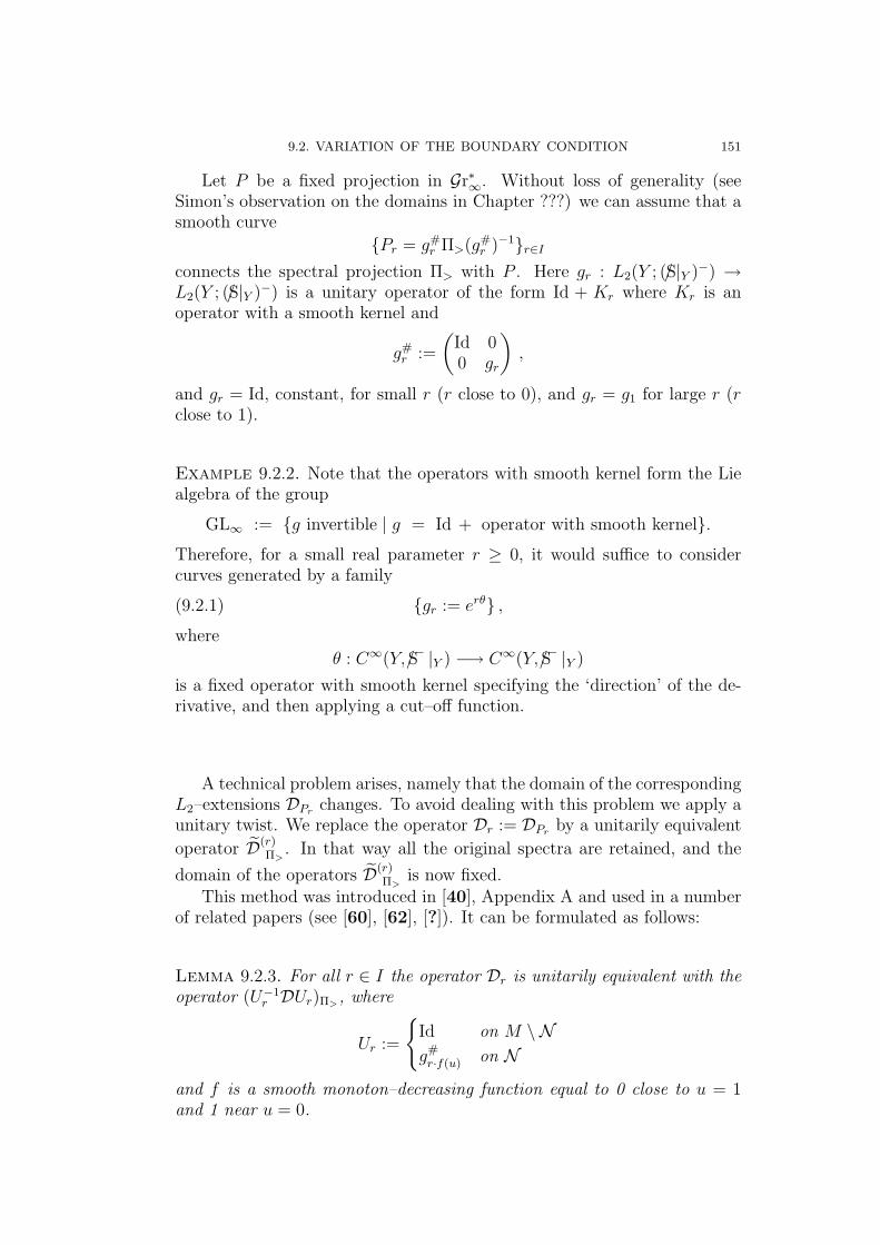
9.2. VARIATION OF THE BOUNDARY CONDITION 151
Let P be a fixed projection in Gr∗∞. Without loss of generality (seeSimon’s observation on the domains in Chapter ???) we can assume that asmooth curve
{Pr = g#r Π>(g#
r )−1}r∈I
connects the spectral projection Π> with P . Here gr : L2(Y ; (S/ |Y )−) →L2(Y ; (S/ |Y )−) is a unitary operator of the form Id + Kr where Kr is anoperator with a smooth kernel and
g#r :=
(Id 00 gr
),
and gr = Id, constant, for small r (r close to 0), and gr = g1 for large r (rclose to 1).
Example 9.2.2. Note that the operators with smooth kernel form the Liealgebra of the group
GL∞ := {g invertible | g = Id + operator with smooth kernel}.
Therefore, for a small real parameter r ≥ 0, it would suffice to considercurves generated by a family
(9.2.1) {gr := erθ} ,
where
θ : C∞(Y, S/− |Y ) −→ C∞(Y, S/− |Y )
is a fixed operator with smooth kernel specifying the ‘direction’ of the de-rivative, and then applying a cut–off function.
A technical problem arises, namely that the domain of the correspondingL2–extensions DPr changes. To avoid dealing with this problem we apply aunitary twist. We replace the operator Dr := DPr by a unitarily equivalent
operator D(r)Π>
. In that way all the original spectra are retained, and the
domain of the operators D(r)Π>
is now fixed.This method was introduced in [40], Appendix A and used in a number
of related papers (see [60], [62], [?]). It can be formulated as follows:
Lemma 9.2.3. For all r ∈ I the operator Dr is unitarily equivalent with theoperator (U−1
r DUr)Π>, where
Ur :=
{Id on M \ Ng#
r·f(u) on N
and f is a smooth monoton–decreasing function equal to 0 close to u = 1and 1 near u = 0.
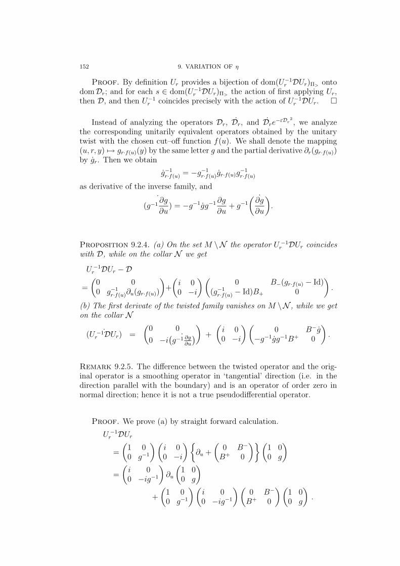
152 9. VARIATION OF η
Proof. By definition Ur provides a bijection of dom(U−1r DUr)Π> onto
domDr; and for each s ∈ dom(U−1r DUr)Π> the action of first applying Ur,
then D, and then U−1r coincides precisely with the action of U−1
r DUr. �
Instead of analyzing the operators Dr, Dr, and Dre−εD 2
r , we analyzethe corresponding unitarily equivalent operators obtained by the unitarytwist with the chosen cut–off function f(u). We shall denote the mapping(u, r, y) 7→ gr·f(u)(y) by the same letter g and the partial derivative ∂r(gr·f(u))by gr. Then we obtain
g−1r·f(u) = −g−1
r·f(u)gr·f(u)g−1r·f(u)
as derivative of the inverse family, and
˙(g−1
∂g
∂u) = −g−1gg−1 ∂g
∂u+ g−1
˙(∂g
∂u
).
Proposition 9.2.4. (a) On the set M \N the operator U −1r DUr coincides
with D, while on the collar N we get
U −1r DUr −D
=
(0 00 g−1
r·f(u)∂u(gr·f(u))
)+
(i 00 −i
)(0 B−(gr·f(u) − Id)
(g−1r·f(u) − Id)B+ 0
).
(b) The first derivate of the twisted family vanishes on M \N , while we geton the collar N
˙(U −1r DUr) =
(0 0
0 −i ˙(g−1 ∂g
∂u
)) +
(i 00 −i
)(0 B−g
−g−1gg−1B+ 0
).
Remark 9.2.5. The difference between the twisted operator and the orig-inal operator is a smoothing operator in ‘tangential’ direction (i.e. in thedirection parallel with the boundary) and is an operator of order zero innormal direction; hence it is not a true pseudodifferential operator.
Proof. We prove (a) by straight forward calculation.
U −1r DUr
=
(1 00 g−1
)(i 00 −i
){∂u +
(0 B−
B+ 0
)}(1 00 g
)=
(i 00 −ig−1
)∂u
(1 00 g
)+
(1 00 g−1
)(i 00 −ig−1
)(0 B−
B+ 0
)(1 00 g
).
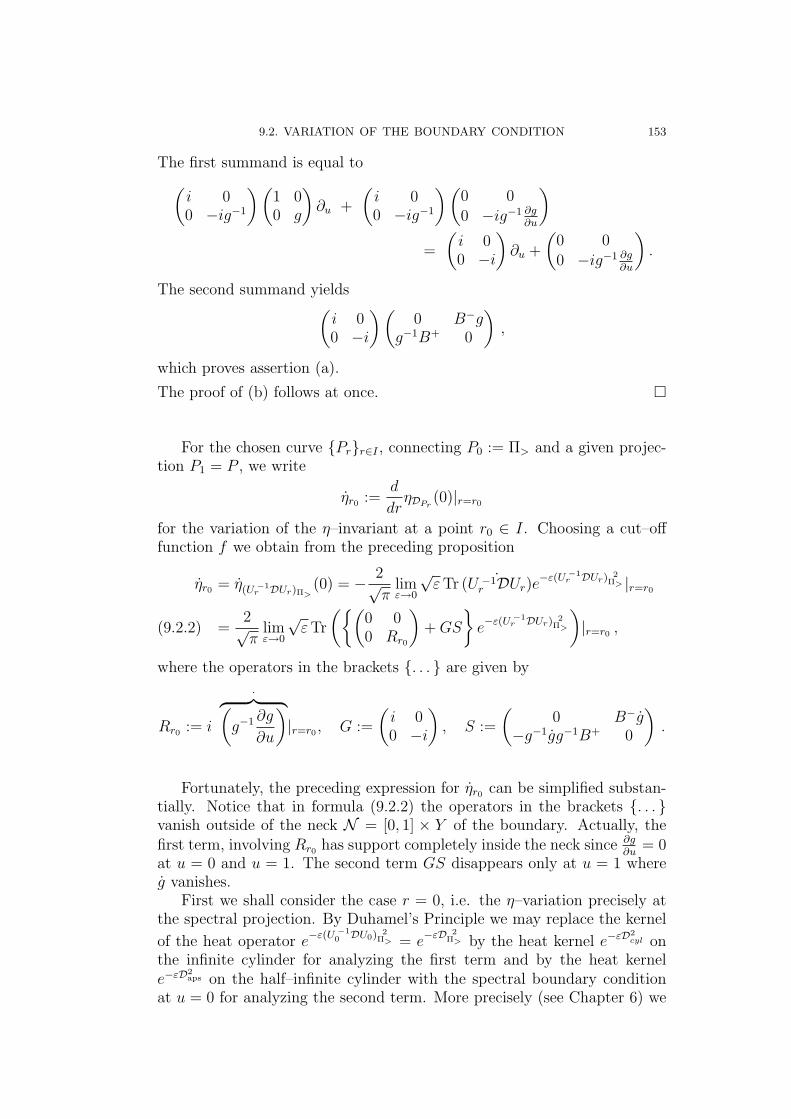
9.2. VARIATION OF THE BOUNDARY CONDITION 153
The first summand is equal to(i 00 −ig−1
)(1 00 g
)∂u +
(i 00 −ig−1
)(0 0
0 −ig−1 ∂g∂u
)=
(i 00 −i
)∂u +
(0 0
0 −ig−1 ∂g∂u
).
The second summand yields(i 00 −i
)(0 B−g
g−1B+ 0
),
which proves assertion (a).
The proof of (b) follows at once. �
For the chosen curve {Pr}r∈I , connecting P0 := Π> and a given projec-tion P1 = P , we write
ηr0 :=d
drηDPr
(0)|r=r0
for the variation of the η–invariant at a point r0 ∈ I. Choosing a cut–offfunction f we obtain from the preceding proposition
ηr0 = η(U −1r DUr)Π>
(0) = − 2√π
limε→0
√εTr ˙(U −1
r DUr)e−ε(U −1
r DUr) 2Π> |r=r0
=2√π
limε→0
√εTr
({(0 00 Rr0
)+GS
}e−ε(U −1
r DUr) 2Π>
)|r=r0 ,(9.2.2)
where the operators in the brackets {. . . } are given by
Rr0 := i
·︷ ︸︸ ︷(g−1 ∂g
∂u
)|r=r0 , G :=
(i 00 −i
), S :=
(0 B−g
−g−1gg−1B+ 0
).
Fortunately, the preceding expression for ηr0 can be simplified substan-tially. Notice that in formula (9.2.2) the operators in the brackets {. . . }vanish outside of the neck N = [0, 1] × Y of the boundary. Actually, thefirst term, involving Rr0 has support completely inside the neck since ∂g
∂u= 0
at u = 0 and u = 1. The second term GS disappears only at u = 1 whereg vanishes.
First we shall consider the case r = 0, i.e. the η–variation precisely atthe spectral projection. By Duhamel’s Principle we may replace the kernel
of the heat operator e−ε(U −10 DU0) 2
Π> = e−εD 2Π> by the heat kernel e−εD2
cyl onthe infinite cylinder for analyzing the first term and by the heat kernele−εD2
aps on the half–infinite cylinder with the spectral boundary conditionat u = 0 for analyzing the second term. More precisely (see Chapter 6) we
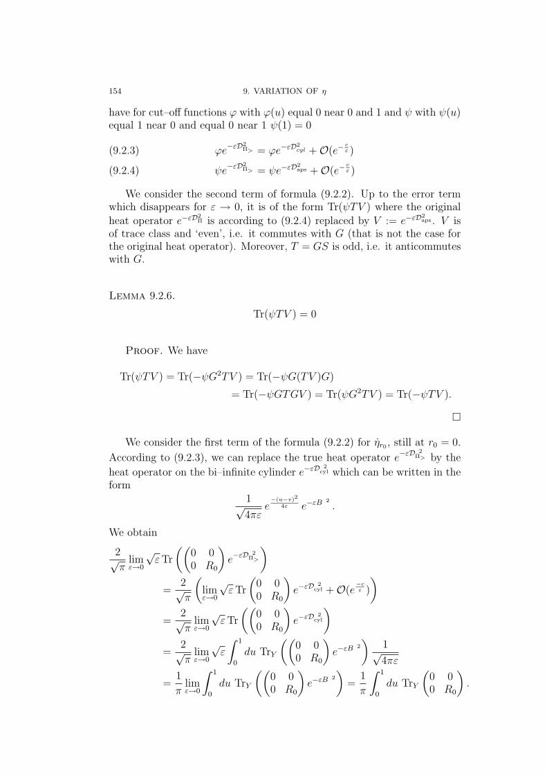
154 9. VARIATION OF η
have for cut–off functions ϕ with ϕ(u) equal 0 near 0 and 1 and ψ with ψ(u)equal 1 near 0 and equal 0 near 1 ψ(1) = 0
ϕe−εD2Π> = ϕe−εD2
cyl +O(e−cε )(9.2.3)
ψe−εD2Π> = ψe−εD2
aps +O(e−cε )(9.2.4)
We consider the second term of formula (9.2.2). Up to the error termwhich disappears for ε → 0, it is of the form Tr(ψTV ) where the original
heat operator e−εD2Π is according to (9.2.4) replaced by V := e−εD2
aps . V isof trace class and ‘even’, i.e. it commutes with G (that is not the case forthe original heat operator). Moreover, T = GS is odd, i.e. it anticommuteswith G.
Lemma 9.2.6.
Tr(ψTV ) = 0
Proof. We have
Tr(ψTV ) = Tr(−ψG2TV ) = Tr(−ψG(TV )G)
= Tr(−ψGTGV ) = Tr(ψG2TV ) = Tr(−ψTV ).
�
We consider the first term of the formula (9.2.2) for ηr0 , still at r0 = 0.
According to (9.2.3), we can replace the true heat operator e−εD 2Π> by the
heat operator on the bi–infinite cylinder e−εD 2cyl which can be written in the
form1√4πε
e−(u−v)2
4ε e−εB 2
.
We obtain
2√π
limε→0
√εTr
((0 00 R0
)e−εD 2
Π>
)=
2√π
(limε→0
√εTr
(0 00 R0
)e−εD 2
cyl +O(e−cε )
)=
2√π
limε→0
√εTr
((0 00 R0
)e−εD 2
cyl
)=
2√π
limε→0
√ε
∫ 1
0
du TrY
((0 00 R0
)e−εB 2
)1√4πε
=1
πlimε→0
∫ 1
0
du TrY
((0 00 R0
)e−εB 2
)=
1
π
∫ 1
0
du TrY
(0 00 R0
).
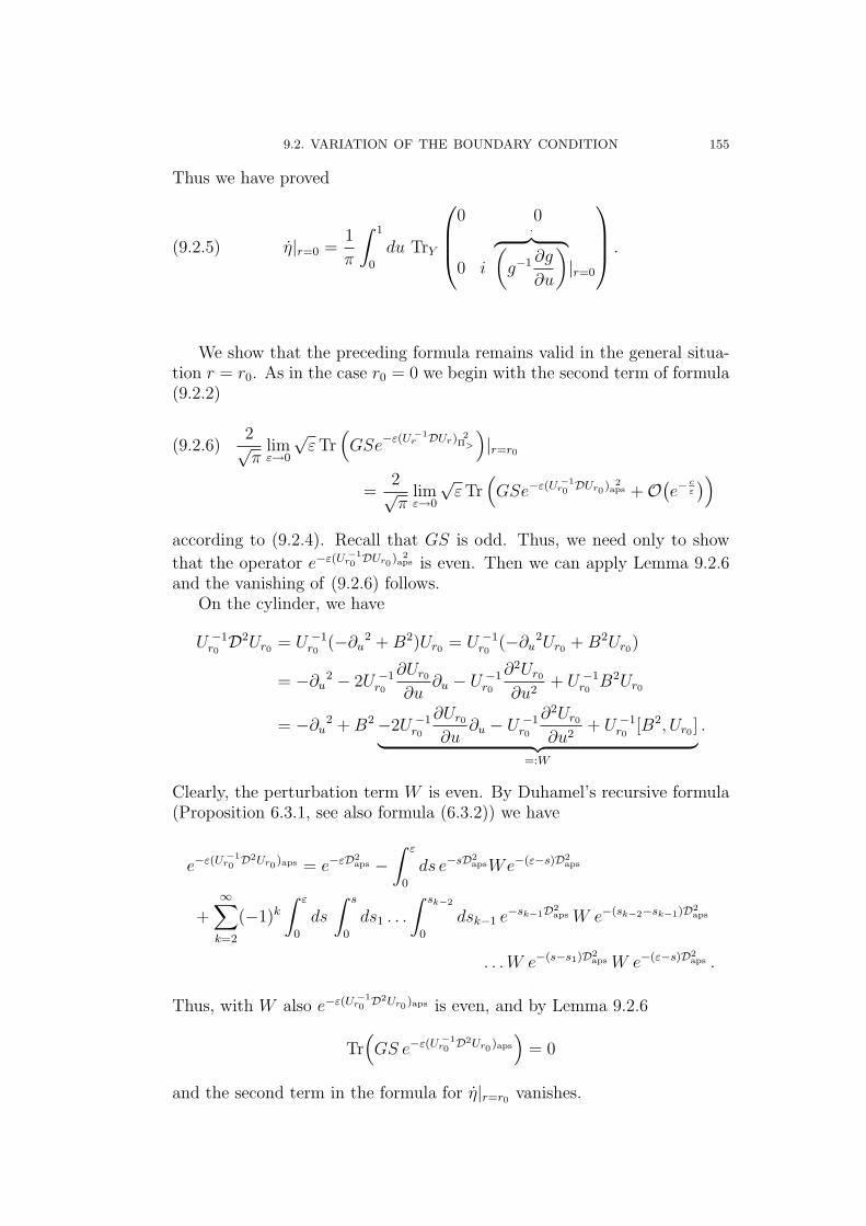
9.2. VARIATION OF THE BOUNDARY CONDITION 155
Thus we have proved
(9.2.5) η|r=0 =1
π
∫ 1
0
du TrY
0 0
0 i
·︷ ︸︸ ︷(g−1 ∂g
∂u
)|r=0
.
We show that the preceding formula remains valid in the general situa-tion r = r0. As in the case r0 = 0 we begin with the second term of formula(9.2.2)
(9.2.6)2√π
limε→0
√εTr
(GSe−ε(U −1
r DUr) 2Π>
)|r=r0
=2√π
limε→0
√εTr
(GSe−ε(U −1
r0DUr0 ) 2
aps +O(e−
cε
))according to (9.2.4). Recall that GS is odd. Thus, we need only to show
that the operator e−ε(U −1r0
DUr0 ) 2aps is even. Then we can apply Lemma 9.2.6
and the vanishing of (9.2.6) follows.On the cylinder, we have
U −1r0D2Ur0 = U −1
r0(−∂u
2 +B2)Ur0 = U −1r0
(−∂u2Ur0 +B2Ur0)
= −∂u2 − 2U −1
r0
∂Ur0
∂u∂u − U −1
r0
∂2Ur0
∂u2+ U −1
r0B2Ur0
= −∂u2 +B2−2U −1
r0
∂Ur0
∂u∂u − U −1
r0
∂2Ur0
∂u2+ U −1
r0[B2, Ur0 ]︸ ︷︷ ︸
=:W
.
Clearly, the perturbation term W is even. By Duhamel’s recursive formula(Proposition 6.3.1, see also formula (6.3.2)) we have
e−ε(U −1r0
D2Ur0 )aps = e−εD2aps −
∫ ε
0
ds e−sD2apsWe−(ε−s)D2
aps
+∞∑
k=2
(−1)k
∫ ε
0
ds
∫ s
0
ds1 . . .
∫ sk−2
0
dsk−1 e−sk−1D2
aps W e−(sk−2−sk−1)D2aps
. . .W e−(s−s1)D2aps W e−(ε−s)D2
aps .
Thus, with W also e−ε(U −1r0
D2Ur0 )aps is even, and by Lemma 9.2.6
Tr(GS e−ε(U −1
r0D2Ur0 )aps
)= 0
and the second term in the formula for η|r=r0 vanishes.
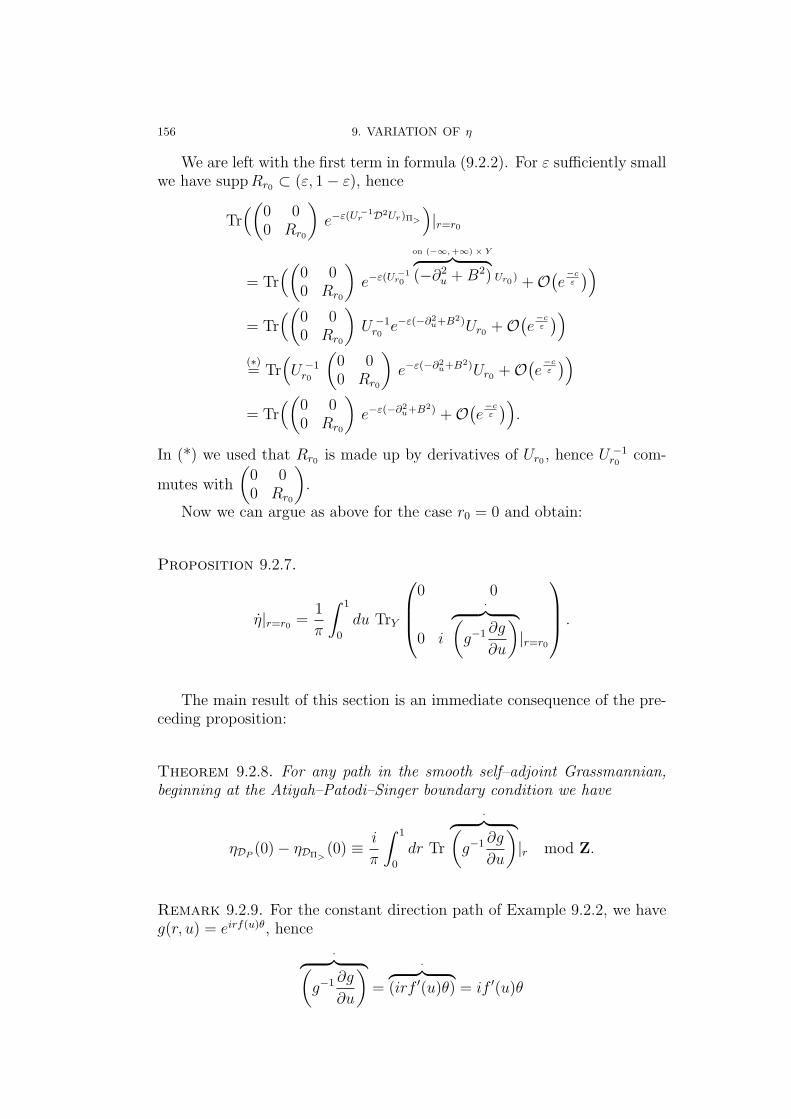
156 9. VARIATION OF η
We are left with the first term in formula (9.2.2). For ε sufficiently smallwe have suppRr0 ⊂ (ε, 1− ε), hence
Tr((
0 00 Rr0
)e−ε(U −1
r D2Ur)Π>
)|r=r0
= Tr((
0 00 Rr0
)e−ε(U −1
r0
on (−∞, +∞)× Y︷ ︸︸ ︷(−∂2
u +B2) Ur0 ) +O(e−cε
))= Tr
((0 00 Rr0
)U −1
r0e−ε(−∂2
u+B2)Ur0 +O(e−cε
))(∗)= Tr
(U −1
r0
(0 00 Rr0
)e−ε(−∂2
u+B2)Ur0 +O(e−cε
))= Tr
((0 00 Rr0
)e−ε(−∂2
u+B2) +O(e−cε
)).
In (*) we used that Rr0 is made up by derivatives of Ur0 , hence U −1r0
com-
mutes with
(0 00 Rr0
).
Now we can argue as above for the case r0 = 0 and obtain:
Proposition 9.2.7.
η|r=r0 =1
π
∫ 1
0
du TrY
0 0
0 i
·︷ ︸︸ ︷(g−1 ∂g
∂u
)|r=r0
.
The main result of this section is an immediate consequence of the pre-ceding proposition:
Theorem 9.2.8. For any path in the smooth self–adjoint Grassmannian,beginning at the Atiyah–Patodi–Singer boundary condition we have
ηDP(0)− ηDΠ>
(0) ≡ i
π
∫ 1
0
dr Tr
·︷ ︸︸ ︷(g−1 ∂g
∂u
)|r mod Z.
Remark 9.2.9. For the constant direction path of Example 9.2.2, we haveg(r, u) = eirf(u)θ, hence
·︷ ︸︸ ︷(g−1 ∂g
∂u
)=
·︷ ︸︸ ︷(irf ′(u)θ) = if ′(u)θ
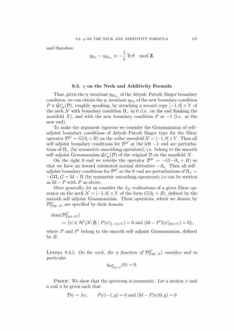
9.3. η ON THE NECK AND ADDITIVITY FORMULA 157
and therefore
ηDP− ηDΠ>
≡ − 1
πTr θ mod Z.
9.3. η on the Neck and Additivity Formula
Thus, given the η–invariant ηDΠ>of the Atiyah–Patodi–Singer boundary
condition, we can obtain the η–invariant ηDPof the new boundary condition
P ∈ Gr∗∞(D), roughly speaking, by attaching a second copy [−1, 0] × Y ofthe neck N with boundary condition Π< in 0 (i.e. on the end flanking themanifold X), and with the new boundary condition P at −1 (i.e. at thenew end).
To make the argument rigorous we consider the Grassmannian of self–adjoint boundary conditions of Atiyah–Patodi–Singer type for the Diracoperator DN = G(∂u +B) on the collar manifold N = [−1, 0]×Y . Then allself–adjoint boundary conditions for DN at the left −1–end are perturba-tions of Π> (by symmetric smoothing operators); i.e. belong to the smoothself–adjoint Grassmannian Gr∗∞(D) of the original D on the manifold X.
On the right 0–end we rewrite the operator DN = −G(−∂u + B) sothat we have an inward orientated normal derivative −∂u. Then all self–adjoint boundary conditions for DN at the 0–end are perturbations of Π< =−GΠ>G = Id− Π (by symmetric smoothing operators); i.e can be writtenas Id− P with P as above.
More generally, let us consider the L2–realizations of a given Dirac op-erator on the neck N = [−1, 0]× Y of the form G(∂u + B), defined by thesmooth self–adjoint Grassmannian. These operators, which we denote byDNP,Id−P , are specified by their domain
dom(DNP,Id−P ′)
:= {ψ ∈ H1(N ; S/) | P (ψ|{−1}×Y ) = 0 and (Id− P ′)(ψ|{0}×Y ) = 0},
where P and P ′ belong to the smooth self–adjoint Grassmannian, definedby B.
Lemma 9.3.1. On the neck, the η–function of DNP,Id−P ) vanishes and inparticular
ηDNP,Id−P(0) = 0.
Proof. We show that the spectrum is symmetric. Let a section ψ anda real λ be given such that
Dψ = λψ, Pψ(−1, y) = 0 and (Id− P )ψ(0, y) = 0
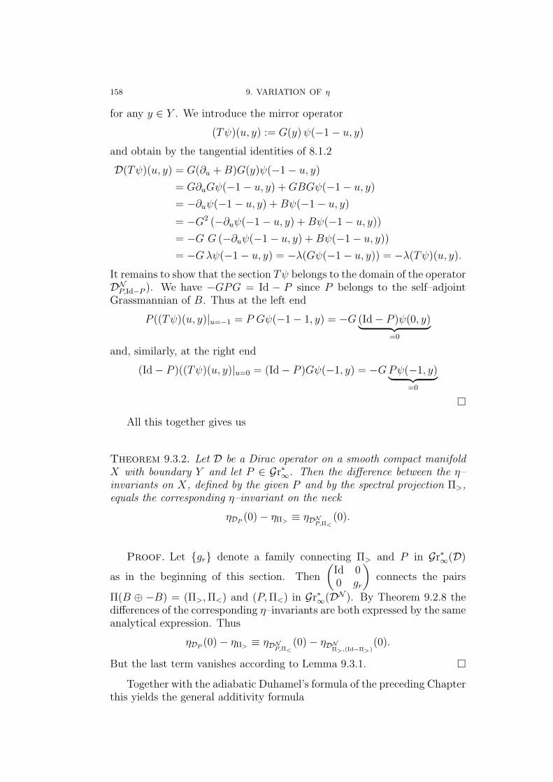
158 9. VARIATION OF η
for any y ∈ Y . We introduce the mirror operator
(Tψ)(u, y) := G(y)ψ(−1− u, y)
and obtain by the tangential identities of 8.1.2
D(Tψ)(u, y) = G(∂u +B)G(y)ψ(−1− u, y)
= G∂uGψ(−1− u, y) +GBGψ(−1− u, y)
= −∂uψ(−1− u, y) +Bψ(−1− u, y)
= −G2 (−∂uψ(−1− u, y) +Bψ(−1− u, y))
= −G G (−∂uψ(−1− u, y) +Bψ(−1− u, y))
= −Gλψ(−1− u, y) = −λ(Gψ(−1− u, y)) = −λ(Tψ)(u, y).
It remains to show that the section Tψ belongs to the domain of the operatorDNP,Id−P ). We have −GPG = Id − P since P belongs to the self–adjointGrassmannian of B. Thus at the left end
P ((Tψ)(u, y)|u=−1 = P Gψ(−1− 1, y) = −G (Id− P )ψ(0, y)︸ ︷︷ ︸=0
and, similarly, at the right end
(Id− P )((Tψ)(u, y)|u=0 = (Id− P )Gψ(−1, y) = −GPψ(−1, y)︸ ︷︷ ︸=0
�
All this together gives us
Theorem 9.3.2. Let D be a Dirac operator on a smooth compact manifoldX with boundary Y and let P ∈ Gr∗∞. Then the difference between the η–invariants on X, defined by the given P and by the spectral projection Π>,equals the corresponding η–invariant on the neck
ηDP(0)− ηΠ> ≡ ηDNP,Π<
(0).
Proof. Let {gr} denote a family connecting Π> and P in Gr∗∞(D)
as in the beginning of this section. Then
(Id 00 gr
)connects the pairs
Π(B ⊕ −B) = (Π>,Π<) and (P,Π<) in Gr∗∞(DN ). By Theorem 9.2.8 thedifferences of the corresponding η–invariants are both expressed by the sameanalytical expression. Thus
ηDP(0)− ηΠ> ≡ ηDNP,Π<
(0)− ηDNΠ>,(Id−Π>)
(0).
But the last term vanishes according to Lemma 9.3.1. �
Together with the adiabatic Duhamel’s formula of the preceding Chapterthis yields the general additivity formula
9.3. η ON THE NECK AND ADDITIVITY FORMULA 159
Corollary 9.3.3. For the η–invariant on a closed partitioned manifoldM = M1 ∪Y M2 with M1,M2 compact manifolds with common boundary Ywe have
ηD = ηD1,P1 + ηD2,−G(Id−P2)G + ηNP1,P2.

Part 4
ζ–Determinant and FredholmDeterminant

CHAPTER 10
The Variation of the Modulus
1
We derive formulas for the change of the modulus of the ζ–determinant of a fixed Dirac operator on a compact smoothmanifold with boundary under variation of the boundary con-dition.
10.1. Introduction
Before deriving our variational formulas of the modulus we shall empha-size the different levels of subtlety of the various spectral invariants involvedinto the definition of the determinant. To begin with we restrict ourselvesto the case of a closed manifold. Recall that the ζ–determinant is given bythe following formula
detD := eiπ2
(ηD(0)−ζD2 (0)) · e−12ζ′D2 (0) .
Let {Dr}r∈I be a smooth family of compatible Dirac operators parametrizedover the interval I = [0, 1]. Then, as noticed before, we have the followingformula for the variation η of the η–invariant ηDr(0)
(10.1.1) η = − 2√π
limε→0
√εTr De−εD2
.
Assuming thatD0 is invertible we find the variation of the modulus−12ζ ′D2(0)
of the determinant:
d
dr
(−1
2ζ ′D2(0)
)=
˙(−1
2
∫ ∞
0
1
te−tD2 dt
)=
∫ ∞
0
Tr DDe−tD2
dt
=
∫ ∞
0
Tr DD−1D2e−tD2
dt =
∫ ∞
0
Tr DD−1 d
dt
(e−tD2
)dt
= limε→0
(Tr DD−1e−tD2
dt)|t=
1ε
t=ε = − limε→0
Tr DD−1e−εD2
.(10.1.2)
Note . Formula (10.1.1) for the variation of the η–invariant requiresthat the family consists of compatible Dirac operators. In the general case,it can be replaced by another formula involving the heat kernel asymptoticsof the operator De−tD2
. Formula (10.1.2) for the variation of the modulusof the ζ–determinant remains valid in the general non–compatible case.
1Date: November 15, 2001. File name: BOOKMOD1.TEX, uses BOOKC.STY andBOOKREFE.TEX.
163
164 10. VARIATION OF THE MODULUS (November 15, 2001)
Notice the very different sensitivity of the various invariants for changesof the underlying data:
• Recall that the index of an elliptic operator depends solely on theprincipal symbol and can be expressed by a local formula. More-over, it is a homotopy invariant of the principal symbol.• The variation η behaves, roughly speaking, like the index because
it is local, i.e. it can be expressed by an integral, and it dependsonly on finitely many terms in the asymptotic expansion of thetotal symbol.• Also the η–invariant depends only on finitely many terms of the
asymptotic expansion of the total symbol of the operator D (or,equivalently, of the inverse D−1), but it is non–local. In particular,it is invariant under perturbation by pseudo–differential operatorsof order less than −m− 1 and other operators of trace class. Here,m denotes the dimension of the manifold.• The same is true for the variation d
dr
(−1
2ζ ′D2(0)
): it depends only
on finitely many terms of the asymptotic expansion of the totalsymbol, thus being a polynomial or, better, an algebraic functionof the total symbol.• Finally, the modulus ζ ′D2(0) of the determinant depends on all
(infinitely–many) terms of the asymptotic expansion of the symbol.As shown before, it can change by perturbation with a smoothingoperator. This is a peculiar aspect of the widely studied non–multiplicativity property of the ζ–determinant .
Assuming that the derivative D is of trace class we get
limε→0
√εTr De−εD2
= 0
and
limε→0
Tr DD−1e−εD2
= Tr DD−1(
limε→0
e−εD2)
= Tr DD−1 .
By (10.1.1) and (10.1.2) it follows
Lemma 10.1.1. Let {Dr} be a smooth family of Dirac operators on a fixedclosed manifold operating on sections in a fixed bundle S of Clifford modulesand let D|r=0 be of trace class. Then we have
η = 0 andd
drln det|D| = d
dr
(−1
2ζ ′D2(0)
)= −Tr DD−1 ,
all taken at r = 0.
The vanishing of η is not surprising since
(10.1.3) ηD(0) = ηD+T (0)
10.1. INTRODUCTION 165
for any T of trace class, as mentioned before. For the modulus of the deter-minant, however, the preceding Lemma shows how delicate the modulus ofthe determinant really is and that it changes even under perturbation by atrace class operator - contrary to the η–invariant which remains accordingto (10.1.3) unchanged under such perturbation.
Having D of trace class is, however, rather untypical. Variation of theconnection would e.g. lead to a perturbation by a bundle endomorphism.Neither a variation of the boundary condition within the Grassmannianwould lead to a D of trace class. Actually, this is a very fortunate instancebecause the more substantial perturbations we are going to consider havethe nice property that they permit the replacement of the precise inverseD−1 by any parametrix for D in the formula (10.1.2).
We proceed with our analysis on a closed manifold M for a short while.We consider a fixed Dirac operator
D : C∞(M ;S) −→ C∞(M ;S)
and a not everywhere vanishing self–adjoint endomorphism V : S → S ofthe fixed bundle S of Clifford modules. Then the family
{Dr := D + rV }, r ∈ [0, 1]
is a smooth family of self–adjoint operators of Dirac type. For r 6= 0,notice that Dr is not necessarily a true (compatible) Dirac operator becausewe admit any endomorphism V which needs not to be compatible withthe Clifford multiplication. For the ease of presentation we assume thatm := dimM is odd, hence ζD2
r(0) = 0.
First we study the variation η. Since V is not of trace class, TrV e−εD2
explodes for ε→ 0. But the factor√ε keeps the trace bounded and gives fi-
nally the result (which replaces (10.1.1) for non–compatible Dirac operators,see our Chapter on the variation of eta)
η =a2m−1√
π.
Here m := dimM and a2m−1 denotes the 2m−1 coefficient in the asymptoticexpansion of the kernel of the operator V e−tD2
.For the variation of the modulus we meet a different situation due to
the absence of the regularizing factor√ε. According to (10.1.2) we have to
determine limε→0 TrVD−1e−εD2. We shall prove the following remarkable
fact:
Proposition 10.1.2. For a family {Dr := D+rV } with self–adjoint bundleendomorphism V the variation of the modulus of the determinant
limε→0
TrVD−1e−εD2
depends only on finitely many terms of the asymptotic expansion of thesymbol of D−1.
166 10. VARIATION OF THE MODULUS (November 15, 2001)
Proof. First we express the integral kernel of the operator D−1 in localcoordinates in terms of the symbol σ(D) = d1 + d0 where d1 denotes theprincipal symbol and d0 the order–0 term. Then we have (see e.g. [45],Lemma 1.7.2.c)
σ(D−1) =∞∑
j=1
q−j
with
q−1 = d−11 and for n > 1
q−n = −q−1
∑|α|+j=n,j<n
Dαξ d0 ·Dα
xq−j/α! +∑
|α|+j=n+1,j<n
Dαξ d1 ·Dα
xq−j/α!
.
By construction, the term q−n is homogeneous of order −n in the covariantvariable ξ.
Locally, the jth term in the expansion of the kernel
K =∞∑
j=1
K−j
of the operator D−1 is completely determined by the jth term q−j in theexpansion of the symbol of D−1:
K−j(x, y) :=
∫ei〈x−y,ξ〉q−j(x, ξ) dξ .
We shall write K−j(x, x − y) instead of K−j(x, y) because the y does notappear as an isolated variable. We show that K−j(x, x−y) is a homogeneousfunction of the argument x− y of order j −m. Recall yhat m denotes thedimension of the manifold M . We have with the variable transformationξ = (ξ1, . . . ξm) 7→ η := rξ
K−j(x, r(x− y)) =
∫ei〈r(x−y),ξ〉q−j(x, ξ) dξ
= r−m
∫ei〈x−y,η〉q−j(x, r
−1η) dη
= r−mr−j(−1)
∫ei〈x−y,η〉q−j(x, η) dη
= rj−m
∫ei〈x−y,η〉q−j(x, η) dη .
In particular we have
K−j(x, x− y) = |x− y|j−mK(x,
x− y|x− y|
).
Next we consider the heat operator e−tD2. It can be expressed in the form
e−tD2
=1
2πi
∫Γ
e−tλ(D2 − λ)−1 dλ .
10.1. INTRODUCTION 167
Expanding the symbol of (D2 − λ)−1 in homogeneous rational functionsshows that the kernel of the heat operator has the following form for smallt > 0 (see e.g. [102], Proposition 13.3)
E(t;x, y) ∼∞∑
k=0
t(k−m)/2pk(x,x− y√
t)e−Qx(x−y)/4t .
Here pk(x, z) are homogeneous polynomials of order k in z and Qx denotesthe positive definite quadratic form
Qx(ξ) = Qx(ξ1, . . . , ξm) = σ2(D2)(x, ξ) =∑
aij(x)ξiξj
given by the principal symbol of the operator D2 at the point x ∈ M . Weshall write E(t;x, x− y) instead of E(t;x, y) because the y does not appearas an isolated variable. We obtain
E(t;x,x− y√
t) ∼ t−m/2
∞∑k=0
|x− y|kpk(x,x− y|x− y|
)e−Qx(x−y)/4t .
We return to our variational formula and find
limε→0
TrVD−1e−εD2
= limε→0
∫dx tr
(V (x)bigl(D−1e−εD2)
(ε;x, x))
= limε→0
∫dx
∫tr(V (x)K(x, x− y)E(ε;x, x− y)
)dy
= limε→0
∫dx trV (x) ·
{ ∑j≥1,k≥0
ε−m/2
∫|x− y|j−mK−j(x,
x− y|x− y|
)|x− y|kpk(x,x− y|x− y|
)e−Qx(x−y)/4ε dy}.
We investigate the sum in the big brackets∑j≥1,k≥0
∫dy |x− y|j+k−mK−j(x,
x− y|x− y|
)pk(x,x− y|x− y|
) ε−m/2e−Qx(x−y)/4ε .
Clearly the factor ε−m/2 will blow up for ε→ 0. Each term in the precedingsum, however, is kept bounded by the Gaussian integral type expression
(10.1.4) limε→0
∫ δ
0
e−a r2
4ε1
2√εdr = lim
ε→0lim
∫ δ/2√
ε
0
e−aζ2
dζ
= lim
∫ ∞
0
e−aζ2
dζ =1
2
√π
a.
If j + k < m, the term |x − y|j+k−m will blow up for small |x − y|.But the variation exists and is finite. So, the whole integral must vanish ifj + k < m.
For a pair (j, k) with j + k > m, the summand∫dy |x− y|j+k−mK−j(x,
x− y|x− y|
)pk(x,x− y|x− y|
) ε−m/2e−Qx(x−y)/4ε
168 10. VARIATION OF THE MODULUS (November 15, 2001)
will, actually, vanish. To prove that we choose a δ > 0 and split the integra-tion domain into |x − y| > δ which is bounded by the manifold’s diameterand |x − y| < δ. For each x, the homogeneous functions K−j(x,
x−y|x−y|) and
pk(x, x−y|x−y|) are actually functions on the unit sphere and hence baunded.
We obtain
limε→0
∣∣∣∫|x−y|>δ
dy |x− y|j+k−mK−j(x,x− y|x− y|
)pk(x,x− y|x− y|
) ε−m/2e−Qx(x−y)/4ε∣∣∣
≤ limε→0
C
∫|x−y|>δ
ε−m/2e−Qx(x−y)/4ε dy and with z =x− y√
ε
≤ limε→0
C
∫|z|> δ√
ε
e−Qx(z)/4 dz = 0.
Similarly we get
limε→0
∣∣∣∫|x−y|<δ
. . . dy∣∣∣ ≤ lim
ε→0dj+k−mC
∫|z|< δ√
ε
e−Qx(z)/4 dz
≤ limε→0
dj+k−mC
∫e−Qx(z)/4 dz = C ′dj+k−m
because of the finiteness of the Gaussian integral. But δ > 0 could be chosenarbitrary small and j + k −m > 0, so also that integral must vanish.
So, only the finitely many terms with j ≥ 1, k ≥ 0, and j + k = mcontribute to the variation
limε→0
TrVD−1e−εD2
= limε→0
∑j+k=m
∫dx trV (x)
∫K−j(x,
x− y|x− y|
)pk(x,x− y|x− y|
)ε−m/2e−Qx(x−y)/4ε dy .
�
Our proposition has two corollaries:
Corollary 10.1.3. (a) For the calculation of the variation of the modulusof the determiant we can replace D−1 by any parametrix Q for D, i.e. anoperator with D−1 −Q is a smoothing operator.(b) The computation of limε→0 TrVD−1e−εD2
localizes.
Proof. (a) is an obvious consequence of the proposition. To prove (b),we consider a smooth partition of unity {Uα, ψα} and define Dα := D|Uα
and Qα := (Dα)−1. Moreover, we set
Q :=∑
α
ϕαQαψα
10.2. VARIATION OF THE ζ-DETERMINANT ON Gr∗∞(D) 169
for suitable bumpfunctions ϕα with ϕα ≡ 1 on Uα). Then we have
Q = D−1DQ = D−1(Id +∑
α
[D, ϕα]Qαψα) ,
henceD−1 = Q−
∑α
D−1[D, ϕα]Qαψα.
The commutator [D, ϕα] has compact support in the complement of Uα,hence disjoint of the support of Qαψα. Therefore, the combined operator[D, ϕα]Qαψα is a smoothing operator, and so is the whole difference D−1 −Q. �
10.2. Variation of the ζ-Determinant on Gr∗∞(D)
In this Section we study the variation of the ζ-determinant of the operatorDP , where P ∈ Gr∗∞(D) , under a change of boundary condition. FromSection 1 we know that the Grassmannian Gr∗∞(D) can be identified withthe group U∞(F−) . If we fix a base projection, for instance P (D), thenany other projection is of the form:
P =
(IdF+ 0
0 g
)P (D)
(IdF+ 0
0 g−1
),
where g : F− → F− is a unitary operator such that g − Id has smoothkernel.
We introduce a smooth one-parameter family {gr}−ε<r<ε of operatorsfrom U∞(F−) with g0 = IdF− . Let {Pr} denote the corresponding familyof projections:
Pr =
(IdF+ 0
0 gr
)P
(IdF+ 0
0 g−1r
).
We want to compute the variation
˙ln detζDPr =d
dr{ln detζDPr}|r=0 .
For the purposes of this paper, it is enough to solve an easier problem.Let us fix two elements of the Grassmannian P1 and P2 such that DP1 andDP2 are invertible operators. The family {gr} determines two 1-parameterfamilies of projections
(10.2.1) Pi,r =
(IdF+ 0
0 gr
)Pi
(IdF+ 0
0 g−1r
)with respect to which we may study the relative variation
170 10. VARIATION OF THE MODULUS (November 15, 2001)
(10.2.2)d
dr{ln detζDP1,r − ln detζDP2,r}|r=0 .
The first obstacle here is that the domains of the unbounded operators DPi,r
are varying with the parameter r. It was explained a long time ago howto solve this problem. We apply a “Unitary Twist” (see [40], [62]). Thepoint is that we may extend the family of unitary isomorphisms {gr} on theboundary sections to a family of unitary transformations {Ur} on L2(M ;S).To do that, fix a smooth non-decreasing function κ(u) such that
κ(u) = 1 for u < 1/4 and κ(u) = 0 for u > 3/4 ,
and for each r introduce the 2-parameter family
(10.2.3) gr,u = grκ(u) for 0 ≤ u ≤ 1 .
Now we define a transformation Ur as follows:
(10.2.4) Ur :=
(IdF+ 0
0 gr,u
)on {u} × Y ⊂ N = [0, 1]× Y
Id on M \N.
We then have the following elementary result
Lemma 10.2.1. The operators DPi,rand (U−1
r DUr)Piare unitary equivalent
operators.
Clearly, the operators Ur depend upon the choice of the extension functionκ, however by Lemma 10.2.1 the ζ-determinant does not, which is all thatwe need. In the following we use the notation
(10.2.5) Dr = U−1r DUr and D0 =
d
drDr|r=0 .
Note that the variation D0 is localized in the collar neighbourhood N ofthe boundary, using the representation (7.1.2) one has
(10.2.6) D0 = GU−1r
{∂
∂uUr + [B, Ur]
}Ur,
where Ur = dUr
drU−1
r .
10.2. VARIATION OF THE ζ-DETERMINANT ON Gr∗∞(D) 171
The Canonical determinant is also independent of the choice of the family{Ur} . This follows from the fact that Pi,rP (D) and the operator PiP (Dr)are unitarily equivalent
(10.2.7)Pi,rP (D) = grPig
−1r P (D) = gr(Pig
−1r P (D)gr)g
−1r = grPiP (Dr)g
−1r .
The main result of this section is the following Theorem:
Theorem 10.2.2. The following equality holds for any pair of projectionsP1, P2 ∈ Gr∗∞(D) such that DP1 and DP2 are invertible operators and for anysmooth 1− parameter family {gr} of operators from U∞(F−) with go = Id:
(10.2.8)d
dr{ln detζDP1,r − ln detζDP2,r}|r=0 = TrD0(D−1
P1−D−1
P2) .
From equations (4.3.8) and (10.2.6) we can write as
d
dr{ln detζDP1,r − ln detζDP2,r}|r=0 =
Tr
(GU−1
r (∂
∂uUr + [B, Ur])UrK
(S(P2)
−1P2 − S(P1)−1P1
)γ0D−1
).
Notice that although the variation D0 is localized in N , the variation ofthe ζ-determinant is not, it depends on global data because of the termD−1
P1−D−1
P2. This is what makes the ζ-determinant a more difficult spectral
invariant than the η-invariant which corresponds to the phase of the deter-minant. Indeed, in the formula (10.2.8) a mathematician working in spectralgeometry will recognize only a variation of the difference of logarithms ofthe modulus of the ζ-determinant. The reason is that the variation of thephase of the determinant of DP1,r is equal to the variation of the phase ofthe determinant of DP2,r .
Theorem 10.2.3. The variation of the phase of the ζ-determinant of theoperator DPr depends only on the family of the unitaries {gr} on F− suchthat
Pr =
(IdF+ 0
0 gr
)P0
(IdF+ 0
0 g−1r
),
172 10. VARIATION OF THE MODULUS (November 15, 2001)
not on the choice of the base-point projection P0 . More specifically ζD2P
(0) isa constant function of the projection P and the variation of the η-invariantdepends only on the family {gr} .
Proof. The Theorem follows from two technical results proved in thework of the second author [113]. The phase of the determinant is equal to
exp{iπ2
(ζD2Pr
(0)− ηDPr(0))} .
It was shown in [113] (Proposition 0.5) that ζD2P
(0) is constant on Gr∗∞(D), hence the variation of the logarithm of the phase is equal to the variationof the η-invariant times −( iπ
2) . The formula for the variation of the η-
invariant was derived in the proof of Theorem 4.3. in [113]. We have
(10.2.9)d
drηDPi,r
(0)|r=0 =i
π
∫ 1
0
du Tr (d
dr(g−1
r,u
∂gr,u
∂u)|r=0) .
In particular the right side of (10.2.9) does not depend on Pi . �
Remark 10.2.4. A special case of the formula (10.2.9) was discussed in thepaper [93].
Next we study the logarithm of the modulus of the determinant
ln |detζDP | = −1
2ζ ′D2
P(0).
It is well-known (see Section 3 of [113]) that
(10.2.10) ζ ′D2P
(0) = lims→0{∫ ∞
0
ts−1Tr e−tD2P dt−
ζD2P
(0)
s} − γ·ζD2
P(0) ,
where γ denotes the Euler constant. The fact that ζD2P
(0) does not depend
on P allows us to study just the variation of the integral in formula (10.2.10)and with the help of Duhamel’s Principle we obtain
d
dr(ζ ′D2
Pi,r
(0))|r=0 =
∫ ∞
0
1
t·Tr(−2tD0DPi
e−tD2Pi )dt =
10.2. VARIATION OF THE ζ-DETERMINANT ON Gr∗∞(D) 173
−2
∫ ∞
0
Tr D0D−1PiD2
Pie−tD2
Pidt = 2
∫ ∞
0
d
dt(Tr D0D−1
Pie−tD2
Pi )dt =
2· limε→0
(Tr D0D−1Pie−tD2
Pi )|1εε = −2· lim
ε→0Tr D0D−1
Pie−εD2
Pi .
We then have the following result:
Lemma 10.2.5.
(10.2.11)d
dr(−1
2ζ ′D2
Pr(0))|r=0 = lim
ε→0Tr D0D−1
Pie−εD2
Pi .
In general the limit on the right hand of the equation (10.2.11) is justthe constant term in the asymptotic expansion of the heat kernel. However,since we discuss the difference (10.2.2), in this situation we actually obtainthe true operator trace:
d
dr{ln detζDP1,r−ln detζDP2,r}|r=0 = lim
ε→0Tr D0D−1
P1e−εD2
P1−limε→0
Tr D0D−1P2e−εD2
P2 =
limε→0
Tr D0(D−1P1−D−1
P2)e−εD2
P1 = Tr D0(D−1P1−D−1
P2) ,
where for the final step we use Corollary 7.3.2. This completes the proof ofTheorem 10.2.2.

CHAPTER 11
Projective equality of the ζ-determinant and Quillendeterminant
In this chapter we show that the ζ-regularized determinantdetζDP is equal to detCDP modulo a natural multiplicativeconstant.
11.1. Introduction
The purpose of this paper is to explain a direct and precise identitybetween the ζ-determinant of a self-adjoint elliptic boundary value problemfor the Dirac operator over an odd-dimensional manifold with boundaryand a regularization of the determinant as the Fredholm determinant of acanonically associated operator over the boundary. We consider an infinite-dimensional Grassmannian of elliptic boundary conditions commensurablewith Atiyah-Patodi-Singer condition. The latter regularization is defined,in the sense explained below, as the ratio of the determinant of the Diracoperator with given elliptic boundary condition to the determinant of theDirac operator with the basepoint chiral spinor boundary condition. It is aregularization canonically constructed from the topology of the associateddeterminant line bundle and hence called the canonical determinant. Thecanonical determinant is a robust algebraic operator-theoretic object, whilethe ζ-determinant is a highly delicate analytic object, and so it is surprisingthat they coincide. (Though, the equality of the torsions mentioned above atleast suggests that the ζ-determinant may be somehow related to Fredholmdeterminants.) Note however that the fundamental multiplicative propertyof the Fredholm determinant (??) does not hold for the ζ-determinant; if L1
and L2 denote two positive elliptic operator of positive order on a Hilbertspace H then in general
detζ L1 L2 6= detζ L1·detζ L2 .
We refer to [61] for a detailed study of the so-called Multiplicative Anom-aly. But this is not contradictory, the canonical determinant is also not mul-tiplicative, due to the process of taking ratios. To formalise the constructionof taking the ratios of determinants used to define the canonical determinantwe need the machinery of the determinant line bundle. This was introducedin a fundamental paper of Quillen [83] for a family of Cauchy-Riemann oper-ators acting on a Hermitian bundle over a Riemann surface, as the pull-back
175
176 11. ζ-DETERMINANT AND QUILLEN DETERMINANT
of the corresponding ‘universal’ determinant bundle over the space of Fred-holm operators on a separable Hilbert space. The determinant line bundleDET comes equipped with a canonical determinant section A 7→ det A,non-zero if and only if A is invertible, where detA lives in the fibre overA, isomorphic to the complex line DET A := ∧maxKer A⊗ ∧maxCoker A. Quillen showed that in this context one can use the ζ-function in orderto construct a natural metric on this bundle and that the curvature of thismetric provides a natural representative of the 1 − st Chern class. Thiswas extended by Bismut and Freed to the context of the families of Diracoperators on closed manifolds (see [17]) and the curvature identified withthe 2-form component of the local families index density. Inspired by theWitten’s work [107], they also studied the holonomy of the correspondingconnection and provided the first proof of the Witten Holonomy Theorem.This result was also proved independently by Jeff Cheeger (see [35]).
The Bismut and Freed construction showed that the ζ-regularizationprovides a natural metric on the determinant bundle, but did not provide astraightforward correspondence between the ζ-determinant and the canon-ical determinant section. The problem is this: Given a non-zero section σof DET one can assign a complex function detσ to the determinant sectionby taking the ratio of the two sections: det A = detσ(A)·σ(A); given thatA is an operator with a ζ-determinant, find σ such that detσ(A) = detζ(A).Clearly the global existence of such a section σ is equivalent to the trivialityof the determinant line bundle. The function detσ may regarded as a reg-ularized determinant defined relative to the ‘basepoint’ σ. In order to linkthis up with Fredholm determinants we use an equivalent construction ofthe determinant line bundle due to Segal. This formalises the idea of defin-ing a regularized determinant by taking the quotient of two comparableoperators.
Associated to the family of elliptic boundary value problems {DP : P ∈Gr∞(D)} one has a determinant line bundle DET (D) over Gr∞(D), asexplained in Section 1, which is non-trivial over Gr∞(D). Further for eachchoice of basepoint P0 ∈ Gr∞(D) one has a smooth family of Fredholmoperators
{SP0(P ) := PP0 : Ran P0 → Ran P P ∈ Gr∞(D)}
with associated (Segal) determinant line bundle DETP0 equipped with itscanonical determinant section P → det SP0(P ) ∈ DetP0(P ), whereDetP0(P )is the determinant line of the Fredholm operator SP0(P ). Moreover, forP0, P1 ∈ Gr∞(D) there is a canonical line bundle isomorphism
(11.1.1) DETP0 = DetP0(P1)⊗DETP1 ,
defined where the operators are invertible by
11.1. INTRODUCTION 177
(11.1.2) det [SP1(P )SP0(P1)] = det SP0(P1)⊗ det SP1(P ) .
The first factor on the right-side of (11.1.1) refers to the trivial bundlewith fibre DetP0(P1). The determinant line bundle of the family of ellipticboundary value problems is classified in this sense by
(11.1.3) DET (D) = DETP (D) ,
where P (D) is the Calderon projection, preserving the canonical determi-nant sections
(11.1.4) det DP ←→ det S(P ) ,
where we have written S(P ) for SP (D)(P ). We may therefore rewrite (11.1.1)fibrewise as
(11.1.5) DET DP = DET DP0 ⊗DetP0(P ) .
We refer to [91] for all these facts.Let σ(DP0) denote the image of the canonical element det SP0(P1) ⊗
det DP0 ∈ DET DP0 ⊗DetP0(P ) under the isomorphism (11.1.5). Relativeto the choice of the basepoint P0, we therefore have two canonical elementsin DET DP , namely det DP and σ(DP0). Thus over the open subset wherethe operators are invertible, according to our earlier discussion we obtaina regularized determinant of DP by taking the quotient of these elements.The point however is to make a canonical choice of the basepoint P0.
In the following, to make the presentation smoother we assume thatker B = {0} . This is in fact not a serious restriction and we can easilyrelax this condition. The point is that now the operators
B± : F± = C∞(Y ;S±)→ F∓ = C∞(Y ;S∓)
are invertible. (We use also F± to denote the space of L2 sections of thebundle of spinors of ”positive′ (resp. ”negative”) chirality.)
Coming back to the canonical choice of the basepoint, in our situationwe are interested just in the real submanifold Gr∗∞(D) of self-adjoint bound-ary conditions and the ‘correct’ choice is indicated by the fact any ellipticboundary condition P ∈ Gr∗∞(D) is described precisely by the property thatits range is the graph of an elliptic unitary isomorphism T : F+ → F−
such that T − (B+B−)−1/2B+ has a smooth kernel.There is a further subtlety that the corresponding orthogonal projection
P+ onto F+ is not actually an element of the Grassmannian. But from
178 11. ζ-DETERMINANT AND QUILLEN DETERMINANT
(11.1.2) the isomorphism (11.1.5) is well-defined if we include the correc-tion factor τ = det(S(P (D))/det[SP (D)(P
+)SP+(P (D))], which introducesa factor of 1/2 in the final formula (see (5.2.6)). The canonical determinantis then defined to be the quotient taken in DET DP
(11.1.6) detCDP =det DP
σ(DP+).
Roughly speaking this is the quotient det DP/det D+P , the precise definition
takes account of the fact that the domains of the operators DP and D+P
are different and hence that their canonical determinant elements live indifferent complex lines. In Section 1 we carry out a precise computationand we see that detCDP is actually the Fredholm determinant of an operatorliving on the boundary Y constructed from projections P and P (D) .Themain result of the paper is the following Theorem:
Theorem 11.1.1. The following equality holds over Gr∗∞(D)
(11.1.7) detζDP = detζDP (D)·detCDP .
Remark 11.1.2. (1) Theorem 11.1.1 shows that, at least on Gr∗∞(D) , theζ-determinant is an object which is a natural extension of the well-definedalgebraic concept of the determinant.
(2) Our results show that the ζ-determinant of the boundary problemDP is actually equal to the Fredholm determinant of the operator S(P )living on the boundary. This extends the corresponding result for the index, which is well-known (see Theorem 20.8 [27]).
(3) With Theorem 11.1.1 at our disposal we can now try a new approachto the pasting formula for the ζ-determinant with respect to a partitioningof a closed manifold. The pasting formula for detC was introduced in [91]. Itis hoped that a new insight into the pasting mechanism of the ζ-determinantwill be obtained by combining results of [91] and formula (11.1.7).
We study the variation of the determinants in order to prove Theorem11.1.1. More precisely, we fix two projections P1, P2 ∈ Gr∗∞(D) such that theoperators DPi
are invertible. Next we choose a family of unitary operatorsof the form
11.1. INTRODUCTION 179
{(IdS+ 0
0 gr
)}0≤r≤1 ,
where gr : F− → F− is a unitary operator, and such that gr − IdF− is anoperator with a smooth kernel for any r , and g0 = IdF− . We define twofamilies of boundary conditions:
Pi,r =
(IdF+ 0
0 gr
)}Pi
(IdF+ 0
0 g−1r
),
and study the relative variation:
d
dr{ln det DP1,r − ln det DP2,r}|r=0 ,
for both the Canonical determinant and the ζ-determinant. Of course weface the technical problem of dealing with a family of unbounded operatorswith varying domain. To circumvent this and make sense of the variationwith respect to the boundary condition we follow Douglas and Wojciechow-ski [40] and apply their ”Unitary Trick”. This defines an extension of ourfamily of unitary operators on the boundary sections to a family {Ur} ofunitary operators acting on L2(M ;S) (see formula (10.2.4)). The operatorDPi,r
is unitarily equivalent to the operator (Dr)Pi, where
Dr = U−1r DUr .
Both the ζ-determinant and the canonical determinant are invariant underthis unitary twist which allows us to compute that both determinants havevariation given by the expression
(11.1.8)d
dr{ln det DP1,r − ln det DP2,r}|r=0 = Tr D0(DP1 −DP2) ,
where D0 denotes the operator ddrDr|r=0. Now we use the fact that the set of
projections P ∈ Gr∗∞(D), such that the operator DP is invertible is actuallypath connected ( see [78]) and integrate the equality
d
dr{ln detζ DP1,r−ln detζ DP2,r}|r=0 =
d
dr{ln detC DP1,r−ln detC DP2,r}|r=0 ,
in order to obtain formula (11.1.7) of Theorem 11.1.1.
180 11. ζ-DETERMINANT AND QUILLEN DETERMINANT
Remark 11.1.3. The reader might think that formula (11.1.8) is incorrectas it does not contain the variation of the phase of the ζ-determinant. Thevariation of logarithm of the modulus of ζ-determinant (at DPi
) is knownto be
limε→0
Tr D0D−1Pie−εD2
Pi ,
and this leads to the right side of (11.1.8), understood as
1
2
d
dr(ln detζ D2
P1− ln detζ D2
P2) .
However, it follows from a result of the work [113], that in the situationstudied in this paper the variation of the phase of ζ-determinant dependsonly on the family of unitaries {Ur} and the operator D . Therefore thephase contributions cancel each other. For more details we refer to Section3.
In Section 1 we explain construction of the Canonical Determinant. Wefollow here the exposition of [91].
Assume that for given P ∈ Gr∗∞(D) the operator DP is invertible. InSection 2 we present our construction of an inverse D−1
P . To do that wehave to discuss certain aspects of the theory of elliptic boundary problems.We also introduce K the Poisson map of the operator D and K(P ) thePoisson map of the operator DP . The first is used in the constructionof the Calderon projection. The operator K(P ) appears in several crucialplaces in our computation of the variation of the Canonical Determinant.
In Section 3 we discuss the variation of the ζ-determinant and in Section4 we study the variation of the Canonical Determinant. It has alreadybeen mentioned that the work [113] was crucial for the study here of theζ-determinant, while in the calculation of the variation of the CanonicalDeterminant we were influenced by the work of Robin Forman [43].
With (11.1.8) at hand, Section 5 contains the final steps of the proof ofTheorem 0.1.
11.2. Variation of the Canonical Determinant
In this section we prove the corresponding result to Theorem 10.2.2 for thecanonical determinant and show that it coincides with the relative variationof the ζ-determinant (10.2.8). We begin with the following result:
11.2. VARIATION OF THE CANONICAL DETERMINANT 181
Proposition 11.2.1. The following formula holds for any P1, P2 ∈ Gr∗∞(D)such that DP1 and DP2 are invertible operators.
(11.2.1) detCDP1,r(detCDP2,r)−1 = detFr
(Id 00 T2T
−11
)Sr(P1)Sr(P2)
−1 ,
where Sr(Pi) denotes the operator PiP (Dr) : H(Dr)→ Ran Pi .
Proof. Let
UT1,T2 =
(Id 00 T2T
−11
): RanP1 → RanP2
and observe that
(11.2.2) UT1,T2UT3,T1 = UT3,T2 , U−1T1,T2
= UT2,T1
and that if A : RanP1 → RanP1 is of the form Id plus trace-class then
(11.2.3) detFr A = detFr U−1T1,T2
AUT1,T2 ,
where the determinant on the left-side is taken on RanP1 and the determi-nant on the right-side is taken on RanP2. Then since U(P ) = UK,T , we haveusing the invariance (10.2.7) of the canonical determinant under a unitarytwist and the multiplicativity (??) of the Fredholm determinant
detCDP1,r(detCDP2,r)−1 = detFr(U−1Kr,T1Sr(P1)) detFr((U
−1Kr,T2Sr(P2))
−1)
= detFr(U−1Kr,T1Sr(P1)S(P2)
−1UKr,T2)
= detFr(U−1Kr,T2
UT1,T2Sr(P1)S(P2)−1UKr,T2)
= detFr(UT1,T2Sr(P1)Sr(P2)−1),
where the last two lines use (11.2.2) and (11.2.3), respectively. �
Hence setting
Sr =
(Id 00 T2T
−11
)P1P (Dr)(P2P (Dr))
−1P2 : Ran P2 → Ran P2
we have proved
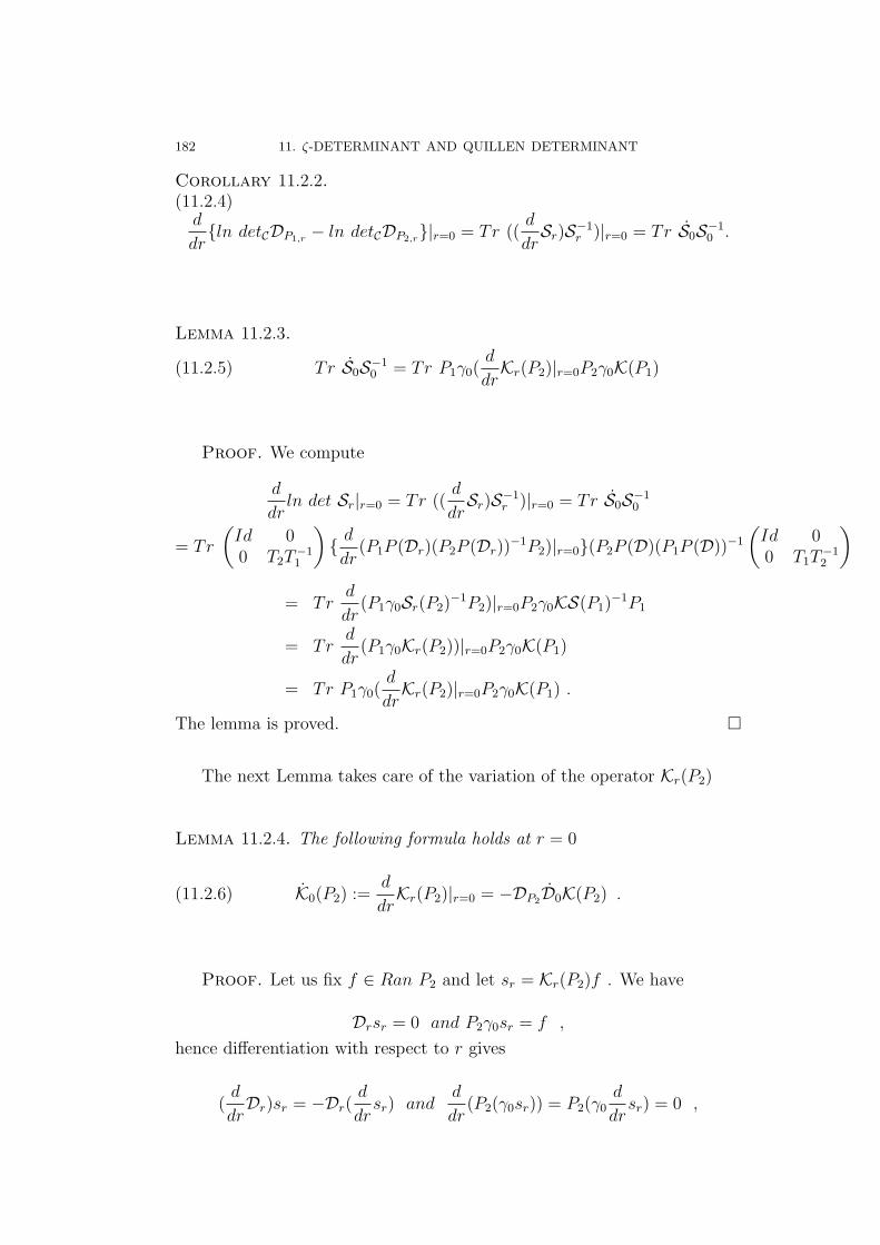
182 11. ζ-DETERMINANT AND QUILLEN DETERMINANT
Corollary 11.2.2.(11.2.4)d
dr{ln detCDP1,r − ln detCDP2,r}|r=0 = Tr ((
d
drSr)S−1
r )|r=0 = Tr S0S−10 .
Lemma 11.2.3.
(11.2.5) Tr S0S−10 = Tr P1γ0(
d
drKr(P2)|r=0P2γ0K(P1)
Proof. We compute
d
drln det Sr|r=0 = Tr ((
d
drSr)S−1
r )|r=0 = Tr S0S−10
= Tr
(Id 00 T2T
−11
){ ddr
(P1P (Dr)(P2P (Dr))−1P2)|r=0}(P2P (D)(P1P (D))−1
(Id 00 T1T
−12
)= Tr
d
dr(P1γ0Sr(P2)
−1P2)|r=0P2γ0KS(P1)−1P1
= Trd
dr(P1γ0Kr(P2))|r=0P2γ0K(P1)
= Tr P1γ0(d
drKr(P2)|r=0P2γ0K(P1) .
The lemma is proved. �
The next Lemma takes care of the variation of the operator Kr(P2)
Lemma 11.2.4. The following formula holds at r = 0
(11.2.6) K0(P2) :=d
drKr(P2)|r=0 = −DP2D0K(P2) .
Proof. Let us fix f ∈ Ran P2 and let sr = Kr(P2)f . We have
Drsr = 0 and P2γ0sr = f ,
hence differentiation with respect to r gives
(d
drDr)sr = −Dr(
d
drsr) and
d
dr(P2(γ0sr)) = P2(γ0
d
drsr) = 0 ,
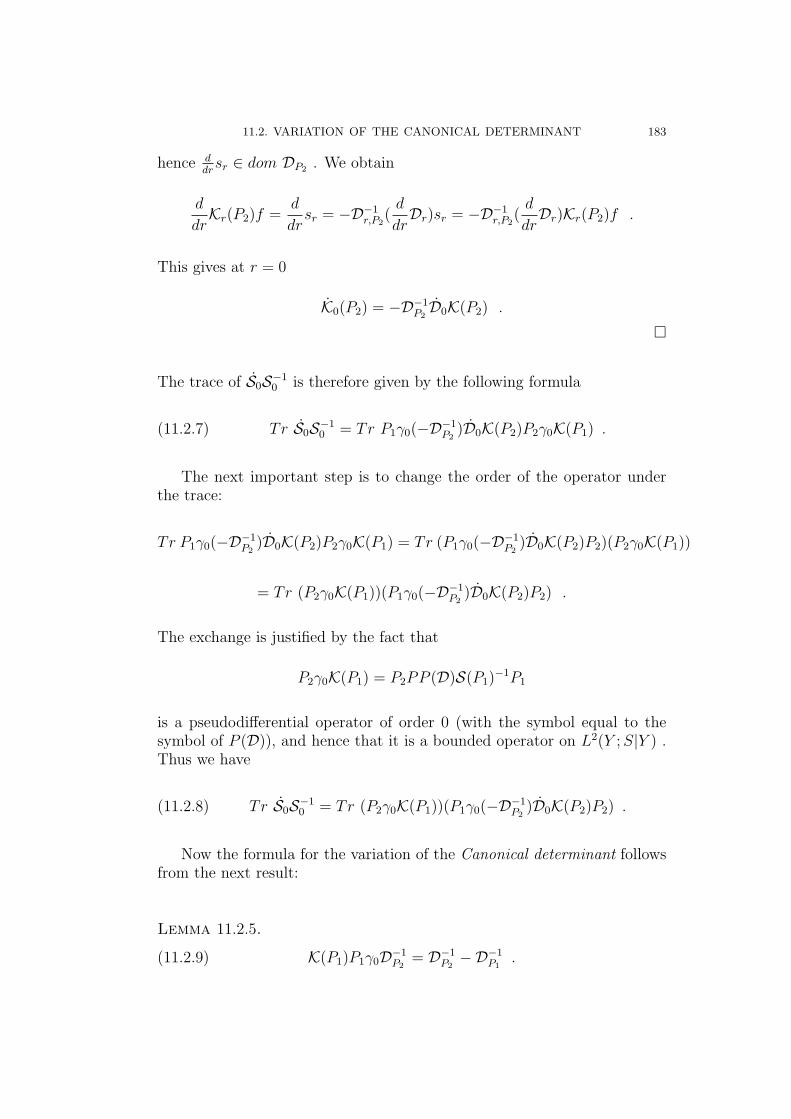
11.2. VARIATION OF THE CANONICAL DETERMINANT 183
hence ddrsr ∈ dom DP2 . We obtain
d
drKr(P2)f =
d
drsr = −D−1
r,P2(d
drDr)sr = −D−1
r,P2(d
drDr)Kr(P2)f .
This gives at r = 0
K0(P2) = −D−1P2D0K(P2) .
�
The trace of S0S−10 is therefore given by the following formula
(11.2.7) Tr S0S−10 = Tr P1γ0(−D−1
P2)D0K(P2)P2γ0K(P1) .
The next important step is to change the order of the operator underthe trace:
Tr P1γ0(−D−1P2
)D0K(P2)P2γ0K(P1) = Tr (P1γ0(−D−1P2
)D0K(P2)P2)(P2γ0K(P1))
= Tr (P2γ0K(P1))(P1γ0(−D−1P2
)D0K(P2)P2) .
The exchange is justified by the fact that
P2γ0K(P1) = P2PP (D)S(P1)−1P1
is a pseudodifferential operator of order 0 (with the symbol equal to thesymbol of P (D)), and hence that it is a bounded operator on L2(Y ;S|Y ) .Thus we have
(11.2.8) Tr S0S−10 = Tr (P2γ0K(P1))(P1γ0(−D−1
P2)D0K(P2)P2) .
Now the formula for the variation of the Canonical determinant followsfrom the next result:
Lemma 11.2.5.
(11.2.9) K(P1)P1γ0D−1P2
= D−1P2−D−1
P1.
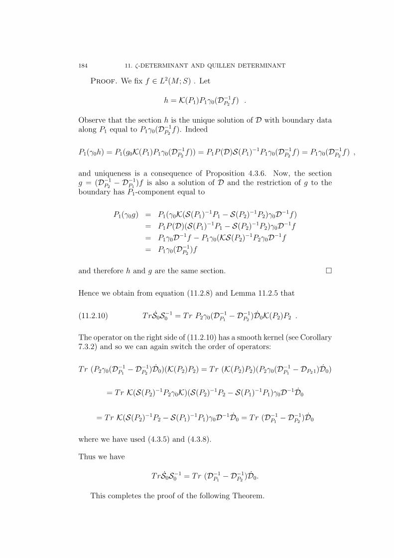
184 11. ζ-DETERMINANT AND QUILLEN DETERMINANT
Proof. We fix f ∈ L2(M ;S) . Let
h = K(P1)P1γ0(D−1P2f) .
Observe that the section h is the unique solution of D with boundary dataalong P1 equal to P1γ0(D−1
P2f). Indeed
P1(γ0h) = P1(g0K(P1)P1γ0(D−1P2f)) = P1P (D)S(P1)
−1P1γ0(D−1P2f) = P1γ0(D−1
P2f) ,
and uniqueness is a consequence of Proposition 4.3.6. Now, the sectiong = (D−1
P2− D−1
P1)f is also a solution of D and the restriction of g to the
boundary has P1-component equal to
P1(γ0g) = P1(γ0K(S(P1)−1P1 − S(P2)
−1P2)γ0D−1f)
= P1P (D)(S(P1)−1P1 − S(P2)
−1P2)γ0D−1f
= P1γ0D−1f − P1γ0(KS(P2)−1P2γ0D−1f
= P1γ0(D−1P2
)f
and therefore h and g are the same section. �
Hence we obtain from equation (11.2.8) and Lemma 11.2.5 that
(11.2.10) TrS0S−10 = Tr P2γ0(D−1
P1−D−1
P2)D0K(P2)P2 .
The operator on the right side of (11.2.10) has a smooth kernel (see Corollary7.3.2) and so we can again switch the order of operators:
Tr (P2γ0(D−1P1−D−1
P2)D0)(K(P2)P2) = Tr (K(P2)P2)(P2γ0(D−1
P1−DP21)D0)
= Tr K(S(P2)−1P2γ0K)(S(P2)
−1P2 − S(P1)−1P1)γ0D−1D0
= Tr K(S(P2)−1P2 − S(P1)
−1P1)γ0D−1D0 = Tr (D−1P1−D−1
P2)D0
where we have used (4.3.5) and (4.3.8).
Thus we have
TrS0S−10 = Tr (D−1
P1−D−1
P2)D0.
This completes the proof of the following Theorem.
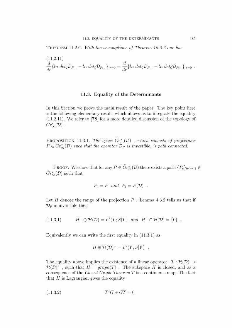
11.3. EQUALITY OF THE DETERMINANTS 185
Theorem 11.2.6. With the assumptions of Theorem 10.2.2 one has
(11.2.11)d
dr{ln detζDP1,r − ln detζDP2,r}|r=0 =
d
dr{ln detCDP1,r − ln detCDP2,r}|r=0 .
11.3. Equality of the Determinants
In this Section we prove the main result of the paper. The key point hereis the following elementary result, which allows us to integrate the equality(11.2.11). We refer to [78] for a more detailed discussion of the topology ofGr∗∞(D) .
Proposition 11.3.1. The space Gr∗∞(D) , which consists of projectionsP ∈ Gr∗∞(D) such that the operator DP is invertible, is path connected.
Proof. We show that for any P ∈ Gr∗∞(D) there exists a path {Pr}0≤r≤1 ∈Gr∗∞(D) such that
P0 = P and P1 = P (D) .
Let H denote the range of the projection P . Lemma 4.3.2 tells us that ifDP is invertible then
(11.3.1) H⊥ ⊕H(D) = L2(Y ;S|Y ) and H⊥ ∩H(D) = {0} .
Equivalently we can write the first equality in (11.3.1) as
H ⊕H(D)⊥ = L2(Y ;S|Y ) .
The equality above implies the existence of a linear operator T : H(D)→H(D)⊥ , such that H = graph(T ) . The subspace H is closed, and as aconsequence of the Closed Graph Theorem T is a continuous map. The factthat H is Lagrangian gives the equality
(11.3.2) T ∗G+GT = 0
186 11. ζ-DETERMINANT AND QUILLEN DETERMINANT
where bundle anti-involution G (see (7.1.2), (7.1.3)) determines symplecticstructure on L2(Y ;S|Y ) . If we now write the projection P with respect tothe decomposition L2(Y ;S|Y ) = H(D)⊕H(D)⊥, we obtain
(11.3.3) P =
((Id+ T ∗T )−1 (Id+ TT ∗)−1T ∗
T (Id+ T ∗T )−1 T (Id+ TT ∗)−1T ∗
).
Since P ∈ Gr∗∞(D) then P − P (D) is a smoothing operator and so theoperator T has a smooth kernel. For each value of the parameter r wedefine the operator Tr = rT and the corresponding projection
Pr =
((Id+ T ∗r Tr)
−1 (Id+ TrT∗r )−1T ∗r
Tr(Id+ T ∗r Tr)−1 Tr(Id+ TrT
∗r )−1T ∗r
).
It is obvious that
ker P (D)Pr∼= coker S(Pr) ∼= Graph(Tr) ∩H(D)⊥ = {0}.
We know that index S(Pr) is equal to 0 and hence that S(Pr) also hasa trivial kernel. The operators Tr satisfy condition (11.3.2), hence Hr =Ran Pr is a Lagrangian subspace satisfying condition (11.3.1). It followsthat the operators DPr are invertible. Moreover P0 = P (D), which ends theproof.
�
The next result is a consequence of Theorem 11.2.6 and Proposition11.3.1.
Proposition 11.3.2. Assume that we have P1, P2 ∈ Gr∗∞(D) and g ∈U∞(F−) such that all four operators DP1, DUP1U−1, DP2, DUP2U−1 are in-vertible, then
(11.3.4)detζDUP1U−1/detCDUP1U−1
detζDP1/detCDP1
=detζDUP2U−1/detCDUP2U−1
detζDP2/detCDP2
.
In particular, the ratio of the determinants does not depend on the choiceof the base projection.
Proof. From Proposition 11.3.1, given any two projections fromGr∗∞(D)such that DP1 and DP2 are invertible operators, we can find a path {Pr} inthe subspace Gr∗∞(D) which connects P1 and P2. Hence we can use Theorem11.2.6 and integrate equation (11.2.11), which gives the identity
11.3. EQUALITY OF THE DETERMINANTS 187
(11.3.5)detζDP1,1/detCDP1,1
detζDP1,0/detCDP1,0
=detζDP2,1/detCDP2,1
detζDP2,0/detCDP2,0
,
where by construction
Pi,1 = gPi,0g−1 = gPig
−1 Pi,0 = Pi .
�
We introduce an invariant A(g) using (11.3.4):
(11.3.6) A(g) =detζDUPU−1/detCDUPU−1
detζDP/detCDP
.
The next result follows from Proposition 11.3.2 and gives the first for-mula directly relating detζ to the detC.
Theorem 11.3.3. There is the following relation between detζ and detC onGr∗∞(D):
(11.3.7) detζDP = detζDP (D)·detCDP ·A(g) ,
where, as before, P =
(Id 00 g
)P (D)
(Id 00 g−1
).
Proof. The result is immediate from the identity (11.3.4) with P1 =
P (D) and P2 = P =
(Id 00 g
)P (D)
(Id 00 g−1
). �
The main result of this Section is the following Theorem.
Theorem 11.3.4. The function A(g) is the trivial character on the groupU∞(F−), i.e. for any g ∈ U∞(F−)
A(g) = 1 .
188 11. ζ-DETERMINANT AND QUILLEN DETERMINANT
Proof. Let g and h be elements of Gr∗∞(D) such that DUgP (D)U−1g
,
DUhP (D)U−1h
and DUhUgP (D)U−1g U−1
hare invertible. We have
A(hg) =detζDUhgPU−1
hg/detCDUhgPU−1
hg
detζDP/detCDP
=
detζDUhgPU−1hg/detCDUhgPU−1
hg
detζDUgPU−1g/detCDUgPU−1
g
·detζDUgPU−1
g/detCDUgPU−1
g
detζDP/detCDP
= A(h)A(g) ,
hence A(g) is a character. It is well-known that there are only two non-trivial characters on the group U∞(F−)
(11.3.8) A+(g) = detFr g and A−(g) = (detFr g)−1 .
We study the variation of detζ at the Calderon projection P (D) to showthat A(g) is actually the trivial character. Let α : F− → F− denote a self-adjoint operator with a smooth kernel. We define the 1-parameter smoothfamily of operators {gr = eirα} in U∞(F−) and the corresponding family ofoperators on M
Ur =
Id on M \N(Id 0
0 eirκ(u)α
)on N
.
with κ as in equation (10.2.3). The variation of the phase of the ζ-determinantis equal to the variation of the η-invariant times the factor −( iπ
2) . It follows
now from formula (10.2.9) that
d
drηDPi,r
(0)|r=0 =i
π
∫ 1
0
du Tr (d
dr(g−1
r,u
∂gr,u
∂u)|r=0) =
i
π
∫ 1
0
du Trd
dr(irκ′(u)α) = −Tr α
π
∫ 1
0
κ′(u)du =Tr α
π,
and so we see that variation of the ζ-determinant in this case is equal to−iTr α
2. On the other hand, the canonical determinant of DgrP (D)g−1
ris
equal to
detCDgrP (D)g−1r
= detFrId+KT−1
r
2= detFr
Id+ e−irα
2
= detFr(e−r iα
2er iα
2 + e−r iα2
2) = detFr(e
−r iα2 cos r
α
2) = e−
ir2
Tr αdetFr(cos rα
2) .
11.3. EQUALITY OF THE DETERMINANTS 189
Therefore the variation of the phase of the canonical determinant is equalto the variation of the phase of the ζ-determinant. From equation (??), thevariation of the only two non-trivial characters (11.3.8) of the group U(F−)are in our case equal to
d
dr(A±(gr))|r=0 = ±i·Tr α ,
and hence A(g) is the trivial character of the group U∞(F−). �
This completes the proof of the main Theorem.

CHAPTER 12
Pasting of Determinants
191

APPENDIX A
The Regularity of the Local η–Function at s = 0
We prove the regularity of the local η–function over a closedmanifold at s = 0, proved first by Bismut and Freed [17] us-ing non–trivial results from stochastic analysis. The details ofour proof are inspired by calculations presented in Bismut andCheeger [14], Section 3.
Theorem A.0.5. Let D : C∞(M ; S/)→ C∞(M ; S/) denote a compatible Diracoperator over a closed manifold M of odd dimension m. Let e(t;x, x′) denote
the integral kernel of the heat operator e−tD2. Then there exists a positive
constant C such that
|trDxe(t;x, x′)|x=x′| < C
√t
for all x ∈M and 0 < t < 1.
We recall the definition of the ‘local’ η–function .
Definition A.0.6. Let {fk;λk}k∈Z be a discrete spectral resolution of D.Then we define
ηD(s;x) :=∑λk 6=0
sign(λk)|λk|−s〈fk(x), fk(x)〉
=1
Γ( s+12
)
∫ ∞
0
ts−12
(∑λk 6=0
λke−tλ2
k〈fk(x), fk(x)〉
)dt
=1
Γ( s+12
)
∫ ∞
0
ts−12 trD e(t;x, x)dt.
Corollary A.0.7. Under the assumptions of the preceding theorem the‘local’ η–function ηD(s;x) is holomorphic in the halfplane <(s) ≥ −2 forany x ∈M .
Proof of the Corollary. . . .�
193
194 A. THE REGULARITY OF THE LOCAL η–FUNCTION AT s = 0
Proof of the Theorem. ****************We follow KPW, On the Bismut-Cheeger proof...
�
Bibliography
[1] Adams, D.H., and Sen, S.: 1996, Partition Function of a Quadratic Functional andSemiclassical Approximation for Witten’s 3–Manifold Invariant. Preprint, TrinityCollege, Dublin.
[2] Atiyah, M.F.: 1985, ‘Eigenvalues of the Dirac operator’; in: Hirzebruch, F. et al.(eds), Arbeitstagung Bonn 1984 , Lecture Notes in Math. 1111, Springer, Berlin, pp.251–260.
[3] —: 1988, ‘Topological quantum field theories’, Inst. Hautes Etudes Sci. Publ. Math.68, 175–186.
[4] —: 1990, The Geometry and Physics of Knots, Cambridge University Press, Cam-bridge, 1990.
[5] Atiyah, M.F., Patodi, V.K., and Singer, I.M.: 1975, ‘Spectral asymmetry and Rie-mannian geometry. I’, Math. Proc. Cambridge Phil. Soc. 77, 43–69.
[6] —, —, —: 1976, ‘Spectral asymmetry and Riemannian geometry. III’, Math. Proc.Cambridge Phil. Soc. 79, 71–99.
[7] Atiyah, M.F., and Singer, I.M.: 1969, ‘Index theory for skew–adjoint Fredholmoperators’, Inst. Hautes Etudes Sci. Publ. Math. 37, 5–26.
[8] —, —: 1984: ‘Dirac operators coupled to vector potentials’, Proc. Nat. Acad. Sci.U.S.A. 81 (1984), 2597–2600.
[9] Avramidi, I.G., and Esposito, G.: 1999, ‘Gauge theories on manifolds with bound-ary’, Comm. Math. Phys. 200, 495–543.
[10] Avron, J.E., Seiler, R., and Simon, B.: 1994, ‘The index of a pair of projections’, J.Funct. Anal. 120, 220–237.
[11] Berline, N., Getzler, E., and Vergne, M.: 1992, Heat Kernels and Dirac Operators,Springer, Berlin.
[12] Bertlmann, R.A.: 1996, Anomalies in Quantum Field Theory, Clarendon Press,Oxford.
[13] Bismut, J.–M., and Cheeger, J.: 1987, ‘Invariants eta et indice des familles pour desvarietes a bord’, C. R. Acad. Sci. Paris Ser. I Math. 305, 127–130.
[14] —, —: 1989, ‘η–invariants and their adiabatic limits’, J. Amer. Math. Soc. 2, 33–70.[15] —, —: 1990a, ‘Families index for manifolds with boundary, superconnections and
cones. I’, J. Funct. Anal. 89, 313–363.[16] —, —: 1990b, ‘Families index for manifolds with boundary, superconnections and
cones. II’, J. Funct. Anal. 90, 306–354.[17] Bismut, J.M., and Freed, D.S.: 1986, ‘The analysis of elliptic families. II. Dirac
operators, eta invariants, and the holonomy theorem’, Comm. Math. Phys. 107,103–163.
[18] Bojarski, B.: 1979, ‘The abstract linear conjugation problem and Fredholm pairs ofsubspaces’, in: In Memoriam I.N.Vekua Tbilisi Univ., Tbilisi, pp. 45–60 (Russian).
[19] Booß, B., and Bleecker, D.D.: 1985, Topology and Analysis. The Atiyah–SingerIndex Formula and Gauge–Theoretic Physics, Springer, New York.
[20] Booß–Bavnbek, B., and Furutani, K.: 1998, ‘The Maslov index: a functional ana-lytical definition and the spectral flow formula’, Tokyo J. Math. 21, 1–34.
195
196 BIBLIOGRAPHY
[21] —, —: 1999, ‘Symplectic functional analysis and spectral invariants’, in: Booss–Bavnbek, B., and Wojciechowski, K.P. (eds.), Geometric Aspects of Partial Differ-ential Equations, Proceedings Roskilde Sept. 1998, Contemporary Mathematics vol.242, Amer. Math. Society, Providence, R.I., pp. 53–83.
[22] Booß–Bavnbek, B., Morchio, G., Strocchi, F., and Wojciechowski, K.P.: 1997,‘Grassmannian and chiral anomaly’, J. Geom. Phys. 22, 219–244.
[23] Booß–Bavnbek, B., Scott, S.G., and Wojciechowski, K.P.: 1998, ‘The ζ–determinantand C–determinant on the Grassmannian in dimension one’, Lett. Math. Phys. 45,353–362.
[24] Booß–Bavnbek, B., and Wojciechowski, K.P.: 1985, ‘Desuspension of splitting ellip-tic symbols. I’, Ann. Global. Anal. Geom. 3, 349-400.
[25] —, —: 1986, ‘Desuspension of splitting elliptic symbols. II’, Ann. Global. Anal.Geom. 4, 337-383.
[26] 1989, ‘Pseudo–differential projections and the topology of certain spaces of ellipticboundary value problems’, Comm. Math. Phys. 121, 1–9.
[27] —, —: 1993, Elliptic Boundary Problems for Dirac Operators, Birkhauser, Boston.[28] Branson, T.P., and Gilkey, P.B.: 1992a, ‘Residues of the eta function for an operator
of Dirac type’, J. Funct. Anal. 108, 47–87.[29] —, —: 1992b, ‘Residues of the eta function for an operator of Dirac type with local
boundary conditions’, J. Differential Geom. Appl. 2, 249–267.[30] Bunke, U.: 1995, ‘On the gluing problem for the η–ivariant’, J. Diff. Geom. 41/2,
397–448.[31] Cappell, S.E., Lee, R., and Miller, E.Y.: 1994, ‘On the Maslov index’, Comm. Pure
Appl. Math. 47, 121–186.[32] —, —, —, ‘Selfadjoint elliptic operators and manifold decompositions Part I: Low
eigenmodes and stretching’, Comm. Pure Appl. Math. 49 (1996), 825–866. ‘PartII: Spectral flow and Maslov index’, Comm. Pure Appl. Math. 49 (1996), 869–909.‘Part III: Determinant line bundles and Lagrangian intersection’, Comm. Pure Appl.Math. 52 (1999), 543–611.
[33] Cheeger, J.:1979, ‘Analytic torsion and the heat equation’, Annals of Math. 109,259–322.
[34] —: 1983, ‘Spectral geometry of singular Riemannian spaces’, J. Diff. Geom. 18,575–657.
[35] —: 1987, ‘η-invariants, the adiabatic approximation and conical singularities’, J.Diff. Geom. 18, 175–221.
[36] Chernoff, P.R.: 1973, ‘Essential self–adjointness of powers of generators of hyperbolicequations’, J. Funct. Anal. 12, 401-414.
[37] Dai, X., and Freed, D.: 1994, ‘η-invariants and determinant lines’, J. Math. Phys.35, 5155–5195.
[38] Dai, X., and Zhang, W.: 1996, ‘Splitting of the family index’, Comm. Math. Phys.182, 303–318.
[39] Douglas, R.G., and Wojciechowski, K.P.: 1989, ‘Analytic realization of relative K-homology on manifolds with boundary and pairing with K-cohomology’, Zeitschriftfur Analysis und ihre Anwendungen 8, 485–494.
[40] Douglas, R.G., and Wojciechowski, K.P.: 1991, ‘Adiabatic limits of the η–invariants.The odd–dimensional Atiyah–Patodi–Singer problem’, Comm. Math. Phys. 142,139–168.
[41] Esposito, G.: 1998, Dirac Operators and Spectral Geometry, Cambridge LectureNotes in Physics vol 12, Cambridge University Press, Cambridge.
[42] —: 1999, ‘Non–local boundary conditions in Euclidean quantum gravity’, Class.Quantum Grav. 16, 1113–1126.
[43] Forman, R.: 1987, ‘Functional determinants and geometry’, Invent. Math.88, 447–493.
BIBLIOGRAPHY 197
[44] Getzler, E.: 1986, ‘A short proof of the local Atiyah–Singer index theorem, Topology25, 111–117.
[45] Gilkey, P.B.: 1995, Invariance Theory, the Heat Equation, and the Atiyah–SingerIndex Theory (Second Edition), CRC Press, Boca Raton, Florida.
[46] Gilkey, P.B., and Smith, L.: 1983a, ‘The eta invariant for a class of elliptic boundaryvalue problems’, Comm. Pure Appl. Math. 36, 85–131.
[47] —, —: 1983b, ‘The twisted index problem for manifolds with boundary’, J. Diff.Geom. 18, 393–444.
[48] Gromov, M., and Lawson, H.B.: 1983, ‘Positive scalar curvature and the Diracoperator’, Publ. Math. Inst. Hautes Etud. Sci. 58, 83–196.
[49] Grubb, G.: 1999, ‘Trace expansions for pseudodifferential boundary problems forDirac–type operators and more general systems’, Ark. Mat. 37, 45–86.
[50] Grubb, G., and Seeley, R.: 1995, ‘Weakly parametric pseudodifferential operatorsand Atiyah–Patodi–Singer boundary problems’, Invent. Math. 121, 481–529.
[51] —, —: 1996, ‘Zeta and eta functions for Atiyah–Patodi–Singer operators’, J. Geo-metric Analysis 6, 31–77.
[52] Hawking, S. W.: 1977, ‘Zeta function regularization of path integrals in curvedspacetime’, Comm. Math. Phys. 55, 133-148
[53] Hitchin, N.: 1974, ‘Harmonic spinors’, Adv. Math. 14, 1–55.[54] Hormander, L.: 1985, The Analysis of Linear Partial Differential Operators III,
Springer, Berlin.[55] Itzykson, C., and Zuber, J.–B.: 1980, Quantum Field Theory , McGraw–Hill, New
York.[56] Janich, K.: 1968, ‘Charakterisierung der Signatur von Mannigfaltigkeiten durch eine
Additivitatseigenschaft’, Invent. Math. 6, 35–40.[57] Karras, U. et al.: 1973, Cutting and Pasting of Manifolds, SK–Groups, Publish or
Perish Inc., Boston.[58] Klein, F.: 1927, Vorlesungen uber die Entwicklung der Mathematik im 19. Jahrhun-
dert. Teil II. Die Grundbegriffe der Invariantentheorie und ihr Eindringen in dieMathematische Physik, Springer, Berlin.
[59] Klimek, S., and Wojciechowski, K.P.: 1993, ‘η–invariants on manifolds with cylin-drical ends’, Differ. Geom. Appl. 3, 191–202.
[60] —, —: 1996, ‘Adiabatic cobordism theorems for analytic torsion and η–invariant’,J. Funct. Anal. 136, 269–293.
[61] Kontsevitch, M. and Vishik, S.: 1993, ‘Geometry of determinants of elliptic opera-tors’. In: Gindikin, S. (ed.) et al., Functional Analysis on the eve of the 21st century’.Vol. I. In honor of the eightieth birthday of I. M. Gelfand. Boston. Birkhauser, Prog.Math. 131, 173–197.
[62] Lesch, M., and Wojciechowski, K.P.: 1996, ‘On the η–invariant of generalizedAtiyah–Patodi–Singer problems’, Illinois J. Math. 40, 30–46.
[63] Luck, W.: 1993, ‘Analytic and topological torsion for manifolds with boundary andsymmetry’, J. Diff. Geom. 37, 263–322.
[64] Matthews, P. T. and Salam, A.: 1954, ‘The Green’s function of quantized field’,Nuovo Cimento Series 9 12, 563–565.
[65] —, —: 1954, ‘Propagators of quantized field’, Nuovo Cimento Series 10 2, 120–134.[66] Mazzeo, R.R., and Melrose, R.B.: 1995, ‘Analytic surgery and the eta invariant’,
GAFA – Geometric And Functional Analysis 5, 14–75.[67] McKean, H., and Singer, I.M.: 1967, ‘Curvature and the eigenvalues of the Lapla-
cian’, J. Diff. Geom. 1, 43–69.[68] Melrose, R.B., and Piazza, P.: 1997, ‘Families of Dirac operators, boundaries and
the b–calculus’, J. Diff. Geom. 46, 99–167.[69] Meyerhoff, R., and Rubermann, D.: 1990, ‘Cutting and pasting the η–invariant’, J.
Diff. Geom. 31, 101–130.
198 BIBLIOGRAPHY
[70] Mickelsson, J.: 1989, Current Algebras and Groups, Plenum Press, New York, 1989.[71] Morchio, G., and Strocchi, F.: 1990, ‘Boundary terms, long range effects, and chiral
symmetry breaking’, in: Mitter, H., and Schweifer, W. (eds.), Fields and Particles,Proceedings Schladming, Austria, 1990, Springer–Verlag, Berlin–Heidelberg–NewYork, pp. 171–214.
[72] Muller, W.:1978, ‘Analytic torsion and R-torsion of Riemannian manifolds’, Adv. inMath. 28, 233–305.
[73] —: 1994, ‘Eta invariants and manifolds with boundary’, J. Diff. Geom. 40, 311–377.[74] —: 1997, ‘On the relative determinant’, Preprint.[75] Nash, C.: 1991, Differential Topology and Quantum Field Theory , Academic Press,
London.[76] Nicolaescu, L.: 1993, ‘The Maslov index, the spectral flow, and splittings of mani-
folds’, C. R. Acad. Sci. Paris 317, Serie I, 515–519.[77] —: 1995, ‘The Maslov index, the spectral flow, and decomposition of manifolds’,
Duke Math. J. 80 (1995), 485–533.[78] —: 1997, Generalized Symplectic Geometries and the Index of Families of Elliptic
Problems, Memoirs of AMS 609, Providence.[79] Palais, R.S. (ed.): 1965, Seminar on the Atiyah–Singer Index Theorem, Ann. of
Math. Studies 57, Princeton University Press, Princeton.[80] Pedersen, G.K., 1989, Analysis Now , Springer, New York.[81] Piazza, P.: 1996, ‘Determinant bundles, manifolds with boundary and surgery’,
Comm. Math. Phys. 178, 597–626.[82] Pressley, A., and Segal, G.B.: 1986, Loop Groups, Clarendon Press – Oxford Uni-
versity Press, Oxford.[83] Quillen, D. G.: 1985, ‘Determinants of Cauchy-Riemann operators over a Riemann
surface’, Funkcionalnyi Analiz i ego Prilozhenya 19, 37–41.[84] Ray, D., and Singer, I.M.: 1971, ‘R–torsion and the Laplacian on Riemannian ma-
nifolds’, Adv. Math. 7, 145–210.[85] Reed, M., and Simon, B.: 1972, Methods of Modern Mathematical Physics. I , Aca-
demic Press, New York.[86] —, —: 1975, Methods of Modern Mathematical Physics, vol II, Academic Press,
New York.[87] —, —: 1978, Methods of Modern Mathematical Physics. IV , Academic Press, New
York.[88] Rees, H.D.: 1984, ‘The η–invariant and Wall non–additivity’, Math. Ann. 267, 449–
452.[89] Roe, J.: 1988, Elliptic Operators, Topology and Asymptotic Methods, Pitman, Lon-
don.[90] Schwarz, A.S.: 1993, Quantum Field Theory and Topology , Springer, Berlin–
Heidelberg–New York. (Russian original: Kvantovaya teoriya polya i topologiya,Nauka, Moscow 1989).
[91] Scott, S.G.: 1995, ‘Determinants of Dirac boundary value problems over odd–dimensional manifolds’, Comm. Math. Phys. 173, 43–76.
[92] Scott, S.G.: ‘Splitting the curvature of the determinant line bundle’, Proc. Am.Math. Soc., to appear.
[93] Scott, S.G., and Wojciechowski, K.P.: 1997, ‘Determinants, Grassmannians andelliptic boundary problems for the Dirac operator’,Lett. Math. Phys. 40, 135–145.
[94] —, —: 1998, ‘ζ-determinant and the Quillen determinant on the Grassmannian ofelliptic self-adjoint boundary conditions’, C. R. Acad. Sci., Serie I, 328, 139–144.
[95] —, —: 1999, ‘The ζ–determinant and Quillen determinant for a Dirac operator ona manifold with boundary’, GAFA (in print).
[96] Seeley, R. T.: 1967 ‘Complex powers of an elliptic operator’. AMS Proc. Symp. PureMath. X. AMS Providence, 288–307.
BIBLIOGRAPHY 199
[97] Seeley, R. T.: 1969, ‘Topics in pseudodifferential operators’. In: CIME Conferenceon Pseudo-Differential operators (Stresa 1968), pp. 167–305. Cremonese 1969.
[98] Segal, G.B.: ‘The definition of conformal field theory’, Oxford preprint, 1990.[99] Shubin, M.A.: 1978, Pseudodifferential Operators and Spectral Theory, Nauka,
Moscow, (Russian, English translation Springer, Berlin, 1986).[100] Singer, I.M.: 1985, ‘Families of Dirac operators with applications to physics’, As-
terisque, hors serie’, 323–340.[101] —: 1988, ‘The η–invariant and the index’, in: Yau, S.–T. (ed.), Mathematical
Aspects of String Theory , World Scientific Press, Singapore, pp. 239–258.[102] Taylor, M.E.: 1996, Partial Differential Equations II - Qualitative studies of Linear
Equations, Springer, New York.[103] Teleman, N.: 1979, ‘Global analysis on PL–manifolds’, Trans. Amer. Math. Soc.
256, 49–88.[104] —: 1984, ‘The index theorem for topological manifolds’, Acta Math. 153, 117–152.[105] Vafa, C., and Witten, E.: 1984, ‘Eigenvalue inequalities for fermions in gauge
theories’, Comm. Math. Phys. 95, 257–274.[106] Wall, C.T.C.: 1969, ‘Non-additivity of the signature’, Invent. Math. 7, 269-274.[107] Witten, E.: 1985, ‘Global gravitational anomalies’, Comm. Math. Phys. 100, 197–
229.[108] —: 1988, ‘Quantum field theory, Grassmannians, and algebraic curves’, Comm.
Math. Phys. 113, 529–600.[109] Wojciechowski, K. P.: 1985, ‘Elliptic operators and relative K − homology groups
on manifolds with boundary’, C. R. Math. Rep. Acad. Sci. Canada 7, 149–154.[110] —: 1988, ‘On the Calderon projections and spectral projections of the elliptic
operators’, J. Operator Theory 20, 107–115.[111] —: 1994, ‘The additivity of the η-invariant: The case of an invertible tangential
operator’, Houston J. Math. 20, 603–621.[112] —: 1995, ‘The additivity of the η-invariant. The case of a singular tangential
operator’, Comm. Math. Phys. 169, 315–327.[113] —: 1999, ‘The ζ-determinant and the additivity of the η-invariant on the smooth,
self-adjoint Grassmannian’, Comm. Math. Phys. 201, 423–444.[114] —: 1997, ‘ζ–determinant, spectral asymmetry and the total symbol of elliptic
operators’ (to appear).[115] —: 1999b, ‘Heat equation and spectral geometry. Introduction for beginners’, in:
Geometric Methods in Quantum Field Theory, Summer School Notes, Villa de Leyva(Colombia), in preparation.
[116] Wojciechowski, K. P., Scott, S. G., Morchio, G., and Booß–Bavnbek, B.: 1998,‘Determinants, manifolds with boundary and Dirac operators’, in: Dietrich, V. etal. (eds.), Clifford Algebras and their applications in mathematical physics’, KluwerAcademic Publishers, pp. 423–432.