the dependence of water permeability in quartz sand on gas
TRANSCRIPT
This article has been accepted for publication and undergone full peer review but has not been through the copyediting, typesetting, pagination and proofreading process which may lead to differences between this version and the Version of Record. Please cite this article as doi: 10.1002/2017JB014630
© 2018 American Geophysical Union. All rights reserved.
The dependence of water permeability in quartz sand on gas hydrate saturation in
the pore space
E. Kossel1, C. Deusner
1, N. Bigalke
1* and M. Haeckel
1
1 GEOMAR Helmholtz Centre for Ocean Research Kiel, Kiel, Germany.
Corresponding author: Elke Kossel ([email protected])
* Present affiliation: GEOTEK, Daventry, UK.
Key Points:
Flow behavior and gas hydrate saturation during CH4 hydrate formation in sand were
monitored.
Different permeability equations were tested for ability to reproduce experimental
results.
Equations of form k ~ (1-SH)n show best agreement with data.
Abstract
Transport of fluids in gas hydrate bearing sediments is largely defined by the reduction of the
permeability due to gas hydrate crystals in the pore space. Although the exact knowledge of
the permeability behavior as a function of gas hydrate saturation is of crucial importance,
state-of-the-art simulation codes for gas production scenarios use theoretically derived
permeability equations that are hardly backed by experimental data. The reason for the
insufficient validation of the model equations is the difficulty to create gas hydrate bearing
sediments that have undergone formation mechanisms equivalent to the natural process and
that have well-defined gas hydrate saturations. We formed methane hydrates in quartz sand
from a methane-saturated aqueous solution and used Magnetic Resonance Imaging to obtain
time-resolved, three-dimensional maps of the gas hydrate saturation distribution. These maps
were fed into 3-D Finite Element Method simulations of the water flow. In our simulations,
we tested the five most well-known permeability equations. All of the suitable permeability
equations include the term (1-SH)n, where SH is the gas hydrate saturation and n is a parameter
that needs to be constrained. The most basic equation describing the permeability behavior of
water flow through gas hydrate bearing sand is k = k0 (1-SH)n. In our experiments, n was
determined to be 11.4 (±0.3). Results from this study can be directly applied to bulk flow
analysis under the assumption of homogeneous gas hydrate saturation and can be further used
to derive effective permeability models for heterogeneous gas hydrate distributions at
different scales.

© 2018 American Geophysical Union. All rights reserved.
1 Introduction
Gas hydrates are crystalline compounds consisting of water molecules enclathrating
small gas molecules. Natural gas hydrates predominantly host methane in the cage structure
and, hence, methane hydrates are considered as an unconventional resource for natural gas
(e.g. [Sloan, 2003]). They are stable at high pressures and low temperatures. On earth,
stability conditions for CH4 hydrates are met in continental margin sediments overlain by at
least several hundred meters of water and below permafrost soil. The US Geological Survey
[2014] provides an updated database on worldwide observations of gas hydrate
accumulations, while numerical diagenetic models are applied to predict global distribution
maps and inventories (e.g. [Buffett and Archer, 2004; Wallmann et al., 2012, Pinero et al.,
2013]). Current estimates of the global amount of methane stored in marine gas hydrates are
roughly 1000 Gt of carbon, equivalent to today’s known conventional reserves of coal, oil,
and natural gas together. This knowledge has triggered the desire to tap this energy resource
and production field trials have been conducted below Arctic permafrost at Mallik in northern
Canada [Dallimore and Collett, 2005; Dallimore et al., 2012] and at Ignik Sikumi in Alaska
[Schoderbek et al., 2013] as well as at the continental slope of the Nankai Trough, Japan
[Cyranoski, 2013]. However, natural gas production from methane hydrate accumulations is
complicated by the fact, that the presence of gas hydrates in the sediment pore space reduces
the permeability of the reservoir. On the other hand, permeability reduction by gas hydrate
formation can be an efficient means to reduce or even prevent leakage of greenhouse gases,
such as CH4 and CO2, through sediments above sub seabed gas reservoirs like conventional
offshore gas production sites and sub-seafloor CO2 storage units. These dynamic changes of
sediment permeability are also a key factor in determining the spatial distribution of gas
hydrate accumulations as well as the temporal evolution of cold seeps by clogging up of gas
migration pathways (e.g. [Luo et al., 2016; Pinero et al., 2016]).
Despite its importance for understanding and predicting mass transport in gas hydrate
settings, it is not well understood in quantitative terms how the formation or dissociation of
gas hydrates in the pore space of marine sediment alters the permeability and consequently
the flow characteristics of the involved phases. Currently, available numerical simulators rely
on theoretical or empirical equations of permeability as a function of gas hydrate saturation
(e.g., [Moridis, 2004; Moridis and Sloan, 2007; Li et al., 2010]) that have not been validated
by data. In this study, we monitored water flow through laboratory-scale sediment samples
during CH4 hydrate formation to test and calibrate published permeability equations.
Magnetic Resonance Imaging (MRI) was employed to obtain spatially and temporally
resolved CH4 hydrate saturations during the formation process. Subsequently, the CH4
hydrate saturation maps were fed into Finite Element Method (FEM) software and different
permeability equations were used to simulate the resulting flow field.
2 Previous studies
Although the knowledge of permeabilities is of utmost importance for the prediction
of the feasibility of gas production from natural gas hydrates, few experimental data for the
validation of permeability equations exist. Laboratory experiments determining permeability
as a function of gas hydrate saturation require precise control of experimental conditions
including the formation of well-defined gas hydrate saturations inside a sediment sample. In
the following paragraphs, we summarize existing theoretically and experimentally derived
permeability models and experimental data sets.

© 2018 American Geophysical Union. All rights reserved.
2.1 Permeability equations
Several permeability equations have been proposed in the literature. Kleinberg et al.
[2003] list a number of equations that were derived from basic geometric considerations: The
pore space of the sediment is approximated either as a bundle of parallel capillaries or as a
Kozeny type grain model [Kozeny, 1927]. Flow obstruction is then calculated for wall- or
grain-coating and center- or pore-filling gas hydrates. For both, the capillary and the grain
model, the equation for water permeability k in the presence of wall-coating gas hydrates has
the form
nHSkk 10 . (1)
In this equation, k0 is the intrinsic permeability in the absence of gas hydrates, SH is the gas
hydrate saturation and n is an exponent that equals 2 for the capillary model. For the grain
model, Spangenberg [2001] derives n = 2.5 by calculating the corresponding Archie
saturation exponent. For center-filling gas hydrates in a capillary bundle, the permeability
equation is
H
HH
S
SSkk
log
121
2
2
0 (2)
whereas pore-filling gas hydrates in a Kozeny grain pack result in
20
1
1
H
n
H
S
Skk
. (3)
Using Spangenberg’s estimation for the Archie saturation exponent, the range for n can be
narrowed down to 2.4 < n < 3.
Further permeability equations, typically used in reservoir simulators, are the van
Genuchten/Parker equation ([Mualem, 1976; van Genuchten, 1980; Parker et al., 1987]), the
Civan equation [Civan, 2001] and the modified Stone equation [Stone, 1970]. Van Genuchten
developed an equation for the hydraulic conductivity of water and gas in unsaturated soils
that is based on equations of Mualem for the prediction of hydraulic conductivities from soil-
water retention curves. Parker and co-workers advanced these equations to a form that is now
routinely used for the description of two-phase flow in soils. The van Genuchten/Parker
equation for the water permeability is
2
1
0 11
nn
WrWr SSkk (4)
where SWr is related to the water saturation SW and the irreducible water saturation SirW of the
soil. In the presence of gas hydrates, Sw depends on gas hydrate saturation:
irW
irWH
irW
irWWWr
S
SS
S
SSS
1
1
1 . (5)
The parameter n in this equation corresponds to 1/n in the original equation. We introduced
this modification in order to have a decrease in permeability with increasing n, similar to the
other listed equations. The van Genuchten/Parker equation was used, for example, by the
EOSHYDR/Tough2 simulator when simulating the Mallik thermal stimulation field test

© 2018 American Geophysical Union. All rights reserved.
[Moridis et al, 2005], and it was chosen for some of the problems in the international gas
hydrate code comparison study initiated by the US Department of Energy [Wilder et al,
2008]. The Civan equation has been derived for fluid flow in a porous medium undergoing
clogging of pores by suspended solid particles or the precipitation of a solid phase. If gas
hydrate formation is considered as the mechanism inducing the clogging of pores, water
permeability is described by the following equation:
n
H
HH
S
SSkk
11
111
0
00
. (6)
Here, denotes the initial porosity of the sediment and n is a parameter that corresponds to
the parameter 2 in the original manuscript. Examples for applications of the equation are
the work of Sun and Mohanty [2006], who used the Civan equation for kinetic simulations of
methane hydrate formation and dissociation in porous media, and of Bai et al. [2008], who
employed it to simulate gas production from a hypothetical marine gas hydrate reservoir.
Stone developed an equation for the calculation of relative permeabilities for three-phase
flow in porous media, including a gas phase, a wetting liquid phase (water) and a non-wetting
liquid phase (oil). For gas hydrate settings, the oil phase is replaced by an immobile hydrate
phase, which allows the calculation of gas/water relative permeabilities (‘modified Stone
equation’). The water permeability is then given by
n
c
cHn
c
c
S
kkk
1
1
0
0
0 (7)
where c is a critical porosity. The critical porosity is the fraction of the pore space that is
occupied by a residual immobile phase. In the case of gas hydrates, c is usually related to
small amounts of free gas that are trapped in the sediment. The modified Stone equation was,
for example, used in the simulation of the Mallik pressure reduction field test [Anderson et al,
2011; Kurihara et al., 2011; Moridis et al., 2011] and the Ignik Sikumi field test [Schoderbek
et al, 2013]. The CMG STARS reservoir simulator (Computer Modelling Group Ltd,
Calgary, Canada) uses a permeability equation for multi-phase flow of the form [CMG, 2009]
2
0
00
11
11
H
n
HS
Skk
. (8)
The software manual describes this equation as a Carman/Kozeny type of equation [Carman,
1937] without giving further details on its derivation.
Besides these theoretically derived equations, also empirical equations have been
proposed. A relatively simple equation is the ‘U-Tokyo equation’ [Masuda et al., 1997],
which equals Eq. 1 and is a simplified form of the modified Stone equation by setting c = 0.
The exponent n is variable and needs to be determined for each geological or experimental
setting. Kurihara et al. [2005] derived permeability equations from a multivariate regression
of the Mallik gas hydrate depressurization production field test data. Their equations have
been fitted only for a limited range of gas hydrate saturations and diverge when SH is
approaching zero. They provide different equations for sand (2 < log(k) < 4)
© 2018 American Geophysical Union. All rights reserved.
776456.3log05075.0
1log59151.0)log(
2
3
HSk
(9)
and for clay (-1 < log(k) < 1).
454054.5log434184.0
1log553688.2)log(
2
3
HSk
.
(10)
The parameters are chosen such that k has the unit mD. Delli and Grozic [2013, 2014]
introduced a weighted sum of the pore-filling and grain-coating versions of the Kozeny grain
equation (Eqs. 1 and 3) where the weighting factors and themselves depend on gas
hydrate saturation:
nHH
H
n
HH SkS
S
SkSk
1
1
1020 .
(11)
Seol and Kneafsey [2011] used X-ray Computed Tomography (X-ray CT) data to determine
gas hydrate saturations in a sediment sample and propose a permeability equation with three
adjustable parameters l, m and n to predict water breakthrough after flooding of the gas-
saturated sample:
HSlnmkk expexp0 .
(12)
2.2 Experimental data
Only limited experimental data for permeabilities in CH4 hydrate-bearing sediments
have been published so far [Kleinberg et al., 2003; Ahn et al., 2005; Minagawa et al., 2005;
Jin et al., 2007; Sakamoto et al., 2010; Johnson et al., 2011; Kneafsey et al., 2011; Liang et
al., 2011; Seol and Kneafsey, 2011; Konno et al., 2013; Li et al., 2013; Schoderbek et al.,
2013; Li et al., 2014]. Most authors have formed gas hydrates in the laboratory by
pressurizing moist sediments with a CH4 gas atmosphere. The bulk gas hydrate saturation
was then calculated from mass balancing by assuming a homogeneous gas hydrate
distribution. The drawback of this approach is that, depending on grain size, the water
distribution in the sample may be homogeneous only for relatively small water contents. As
soon as gravitational forces exceed capillary forces, water will accumulate at the bottom of
the sediment column. Furthermore, at small water saturations, the water forms a wetting film
around the sediment grains. This leads to the preferential formation of grain-coating or pore-
throat blocking gas hydrates whereas natural gas hydrates are believed to be dominantly pore-
filling [Waite et al., 2009]. Kleinberg et al. [2003] and Johnson et al. [2011] formed gas
hydrates by bubbling methane gas through water-saturated sediments. This method is more
similar to formation processes at cold vents, but it is highly unlikely that it will result in
spatially homogeneous gas hydrate formation. Natural gas hydrates have been investigated in
the work of Li et al. [2014], who used pressure core samples from the South China Sea, and
Jin et al. [2007], who worked with pressure core samples from the Nankai Trough.
Ensuring spatially homogeneous gas hydrate saturations is crucial for the
interpretation of the experimental data if only the total amount of gas hydrate is known. If
© 2018 American Geophysical Union. All rights reserved.
spatial homogeneity cannot be guaranteed, the gas hydrate distribution has to be known.
However, only four of the above mentioned experiments applied imaging techniques to
measure spatially resolved gas hydrate saturations: Jin et al. [2007] used X-Ray CT to
characterize the pore space of the gas hydrate-free sediment, but not of the gas hydrate
bearing sediment. Schoderbek et al. [2013] performed MRI and Kneafsey et al. [2011]
employed X-Ray CT to measure averaged one-dimensional gas hydrate saturation profiles,
while Seol and Kneafsey [2011] used X-Ray CT to generate three-dimensional gas hydrate
saturation maps. In the majority of the published studies, permeability was evaluated
exclusively by measuring the pressure drop across the hydrate-bearing sample during fluid
flow. Exceptions are Konno et al. [2013] and Seol and Kneafsey [2011], who used their X-
Ray CT setup to additionally monitor and analyze the intrusion of water into a water-free
hydrate-bearing sediment sample, whereas Li et al. [2014] and Kleinberg et al. [2003] applied
an empirical equation to calculate gas hydrate saturation and permeabilities from Nuclear
Magnetic Resonance (NMR) relaxometry data. Measuring the permeability of pure water or
brine in CH4 hydrate bearing samples has a severe experimental drawback: The fluid is
undersaturated with respect to CH4. It is striving towards thermodynamic equilibrium by
dissolving gas hydrates, causing the permeability to increase during the measurement. In
addition, methane gas may have remained inside the sample despite elaborate flushing
procedures. The presence of the gas can cause additional gas hydrate formation when coming
into contact with the water phase. As a consequence, gas hydrate saturations might not be
constant during permeability measurements. Minagawa et al. [2005], Jin et al. [2007],
Sakamoto et al. [2010], Johnson et al. [2011], Kneafsey et al. [2011] Konno et al. [2013] and
Li et al. [2013] measured water permeabilities with pure water or brine, whereas Seol and
Kneafsey [2011] were seeking to prevent dissolution effects by performing their experiments
with CH4-saturated water. The experiments of Li et al. [2014] and Kleinberg et al. [2003]
were conducted without water flow. Liang et al. [2011] and Schoderbek et al. [2013] solely
measured gas phase permeabilities from single phase gas flow. In order to avoid the
aforementioned experimental difficulties and flaws, we designed an experimental set-up that
allowed us to form gas hydrates from a CH4-saturated water phase while monitoring the 3-
dimensional spatial distribution of gas hydrate saturation with MRI. Data evaluation was
achieved by a full 3-D time-dependent FEM simulation that accounted for the spatially
inhomogeneous formation of gas hydrates.
3 Experimental set-up and data evaluation
3.1 Sample preparation
Quartz sand (G20TEAS, Schlingmeier, Schwülper, Germany) with a mean grain size
of 0.29 mm, a maximum grain size of 0.7 mm, a minimum grain size of 0.063 mm and modal
grain size distribution was packed into a cylindrical sapphire tube with an inner diameter of
1.2 cm and a length of 12 cm. The sand was compacted by vibrations. A piece of a sponge
was inserted on top of the sand to confine the sediment volume and prevent the sand from
moving upstream. The tube was closed with a polyether ether ketone (PEEK) cap, and 1.6
mm (1/16 inch) diameter PEEK capillaries were connected to the caps at both ends of the
tube. To prevent sand grains from moving into the capillaries, filter elements were screwed
into in the end caps. A sketch of the setup is shown in Figure 2a). A vacuum pump was used
to saturate the sand with deionized water. Due to geometric constraints, pressure was
recorded approximately 50 cm upstream and downstream of the sample cell. Therefore, the
measured flow resistance for the gas hydrate free sample was dominated by the flow
resistance of the capillary connections. Connections were sealed with finger-tightened PEEK
© 2018 American Geophysical Union. All rights reserved.
ferrules, which had to be opened between experiments. It is not possible to tighten these
ferrules in a reproducible way. Hence, it is not possible to determine the permeability
contribution of the empty sample cell and its periphery because the retightening of the
ferrules after filling the cell with sediment changes the flow resistance. This effect can be
observed in Figure 3, where both experiments show different initial pressure differences.
Thus, the initial permeability of the sand matrix had to be measured with a separate set-up
that incorporated a larger sand volume: A cylindrical tube with a diameter of d=1.5 cm, a
cross-section of A=7.07 cm2 and a length of l =41.5 cm was filled with compacted quartz
sand. Subsequently, a vacuum pump was used to saturate the sand with deionized water at
room temperature (20 °C). Pressure was measured directly at the bottom and the top of the
sand column. Water was pumped through the column from bottom to top with a high-
performance liquid chromatography (HPLC) pump. Flow rates Q were ranging from 1 to 9.95
ml/min and the corresponding pressure differences ps across the sample length were
recorded after the pressure values had stabilized. Measurements were repeated up to 4 times
and averaged. Additionally, pressure differences pw were measured for the same set-up
without sand. Slope values ps,w/Q were determined by fitting the two datasets with a linear
function (Fig. 1). The values for Q=0 ml/min and Q=1ml/min were left out in the fit because
the HPLC pump works more reliable at higher flow resistances. Using the derived slope
values, the sample permeability was calculated from Darcy’s law
AQ
p
Q
p
lk
ws
(13)
where is the dynamic viscosity of water. Porosity was calculated from the sand volume Vs,
which was calculated from the weight of the sand sample and the density of the sand grains,
and the tube volume V=Al:
V
VV s
(14)
The porosity of the sand sample was 0.35 and the permeability was 3.4×10⁻¹¹
m2 or
34 Darcy.
3.2 Gas hydrate formation
The sapphire tube containing the sample was inserted into a PEEK cooling jacket,
mounted in upright position inside a NMR spectrometer (400 MHz Avance III, Bruker
Biospin, Rheinstetten, Germany) and connected to our high-pressure flow-through system
NESSI [Kossel et al., 2013b]. A HPLC pump (SYKAM, Fürstenfeldbruck, Germany) was
used to pressurize the sample with deionized water to 12 MPa. The sample cooling was
adjusted to maintain a sample temperature of 5 °C. In order to prevent gas hydrate formation
outside of the sand sample, the capillary connectors at the PEEK caps were heated with warm
air. The gas-saturated fluid for gas hydrate formation was prepared by filling deionized water
into a stirred pressure vessel (Parr Instrument Company, Moline, USA) and exposing it to a
12 MPa CH4 atmosphere (purity 99.995 %, AirLiquide, Kornwestheim, Germany) at room
temperature. The water/gas system was allowed to equilibrate for more than 24 hours. Then,

© 2018 American Geophysical Union. All rights reserved.
the fluid supply for the sample was switched from deionized water to CH4-saturated water.
Saturation concentrations for methane in water were calculated with dedicated routines
[Kossel et al., 2013a] programmed in the MATLAB® environment (The Mathworks, Nattick,
USA). They correspond to 0.123 mol/kg at 12 MPa, 22 °C and 0.165 mol/kg at 12 MPa, 5 °C
[Duan and Mao, 2006]. In the presence of gas hydrates, the saturation concentration
decreases to 0.077 mol/kg (12 MPa, 5 °C) [Tishchenko et al., 2005]. The fluid was pumped
through the sample from bottom to top with a constant flow rate of 0.75 ml/min. Gas hydrates
formed from the CH4-saturated water phase with no free gas being present in the sand
sample. The formation started at random times, but mostly within 48 hours after starting the
inflow of gas-saturated water. The experiment was automatically terminated when the
pressure increase due flow obstruction caused by gas hydrate formation resulted in upstream
pressures of more than 15 MPa. This termination condition corresponds to the maximum
allowed pressure for a safe operation of the sample cell. Pressure was measured upstream and
downstream of the sample cell and the difference of these experimentally derived pressures
was calculated. These data are hereafter referred to as “experimentally derived pressure
differences”.
3.3 Magnetic Resonance Imaging (MRI)
We used hydrogen MRI [Callaghan, 1993; Weishaupt, 2008] to monitor the growth
and spatial distribution of CH4 hydrate in the quartz sand sample. MRI solely detects mobile
molecules, i.e. it images the hydrogen in the liquid water phase but not the solid gas hydrate
or sediment phases. The presence of gas hydrates can only be deduced indirectly from a local
absence of the water signal. Water with dissolved CH4 gas was pumped through the sample
for 30 minutes. Then, the flow was stopped and a set of 3-D images was recorded that
covered the entire sediment sample. The length of the radio frequency (RF) resonator for
imaging was 4 cm. This is relatively small compared to the length of the sample tube (12
cm). Therefore, a stepping motor was used to reposition the sample between measurements
for a piecewise imaging of the total sand column. The images were merged to a single dataset
and served as reference image of the gas hydrate free sample. For these measurements, a
multi-slice multi-spin echo sequence (MSME) with a repetition time TR of 10 s, an echo time
TE of 3 ms and 32 collected echoes was applied. The field of view (FOV) was 1.5 × 1.3 cm2
with an in-plane spatial resolution of 0.235 × 0.235 mm2. The sample volume was covered by
26 image slices with a slice thickness of 0.5 mm. Subsequent to the data acquisition, the multi
echo signal was used to perform a correction for signal loss due to transverse relaxation.
After acquisition of the reference image, the sample was positioned in a way that the
following imaging sequences covered the volume close to the fluid inflow. In order to obtain
a reasonable time resolution, the sample was not repositioned between measurements during
this part of the experiment. A series of T2-weighted multi slice spin echo (MSSE) sequences
was started producing a full 3-D dataset of the volume of interest every 128 s. The
experiment was performed with the following parameters: TR = 4 s, TE = 2.9 ms, FOV = 3 ×
1.3 cm2, spatial resolution 0.94 × 0.4 mm
2, number of slices NS = 13, slice thickness d = 1
mm. After completion of the first two datasets, the fluid flow was resumed and the
experiment was run until finally the flow obstruction due to massive gas hydrate formation
resulted in upstream pressures above 15 MPa and the experiment was automatically
terminated. When the water flow had stopped, a second set of relaxation corrected MSME
images was created with a similar pulse sequence as for the gas hydrate free sample. Gas
hydrate saturation SH was calculated by quantifying the signal loss relative to the gas hydrate
free reference image:

© 2018 American Geophysical Union. All rights reserved.
0
0
I
IISH
(15)
Here, I0 is the signal intensity of the reference image and I is the signal intensity of the
images during CH4 hydrate formation. This equation is valid if gas hydrate formation is the
only source of signal loss. Other possible reasons for signal losses that occur in the course of
the experiment are changes in longitudinal and transverse relaxation behavior: The presence
of gas hydrates in a pore space can alter the relaxation characteristics of the pore water
molecules [Kleinberg et al., 2003]. This effect has in part been accounted for by calibrating
the non-relaxation-corrected MSSE images with gas hydrate saturations that have been
calculated from relaxation-corrected MSME images. For each CH4 hydrate saturation map,
the corresponding experimental pressure difference was defined as the mean measured
pressure difference that was derived from averaging of the pressure data over the acquisition
time of the map (128 s). In contrast to the MSME dataset, the time-resolved MSSE images
covered only the bottom part of the sample. Hence, evaluation of these data was only
possible, if gas hydrates formed primarily in this lower section of the sample. The CH4
hydrate saturation maps of the entire sample that were calculated from the MSME images
were inspected for gas hydrate formation outside the limited image volume of the MSSE
images. Experiments with substantial gas hydrate formation outside the defined volume of
interest in the MSSE images were discarded. This applied to six out of eight experiments,
leaving two datasets for further evaluation. The final gas hydrate saturations of the two
remaining experiments are shown as supplements S1 and S2. In one of the two experiments
(hereafter termed as experiment 1), the position of the FOV was changed during the
experiment. At the time of the change, the new volume of interest contained already a small
spot of CH4 hydrate and the MSSE reference image was not completely gas hydrate free. The
CH4 hydrate spot was identified in the MSME images and the MSSE images were corrected
accordingly. Experiment 2 was performed with a slightly different image resolution than
experiment 1. The geometry parameters were FOV = 3 × 1.3 cm2, in plane spatial resolution:
0.235 × 0.4 mm2, NS = 13, d = 1 mm for the MSME and FOV = 3 × 1.3 cm
2, in plane spatial
resolution: 0.47 × 0.4 mm2, NS = 13, d = 1 mm for the MSSE sequences.
3.4 Finite Elements Method simulations
FEM simulations of the flow field were performed with the software package
COMSOL® Multiphysics (COMSOL, Palo Alto, USA) in the “free and porous media flow”
mode. An 18.5 mm long section of the sample cell was chosen as model domain. The
simulated geometry covers the conical interior volume of the lower end cap and a 10 mm
long cylindrical part of the sapphire tube, which has a diameter of 12 mm and is shown in
Figure 2 b). At first, the measured gas hydrate saturation maps were implemented into the
model: The 30 mm long time-dependent experimental maps were cut to match the size of the
model domain. We specified thresholds to minimize the influence of noise at low signal
strengths or low gas hydrate concentrations. Voxels with reference signal amplitudes or
calculated gas hydrate saturations below the corresponding threshold values were defined to
be free of gas hydrates. Thresholds were chosen for each dataset individually according to the
corresponding signal to noise level of the data. Apparent decreases of gas hydrate saturation
at isolated grid points in time and space, which are associated with noise-related fluctuations
of the signal, were removed from the data. The final nine experimental gas hydrate saturation
maps of each selected experiment were included in the FEM simulations in the form of

© 2018 American Geophysical Union. All rights reserved.
interpolation functions. This selected time frame covers the period of severe pressure increase
in the experiments. The internal interpolation routine of COMSOL® Multiphysics tends to
smooth out steep gradients or, in extreme cases, even to make them vanish locally. Since
there is no other possibility to import our experimental data into the software, we pre-treated
the data before feeding them into the simulation software: The grid of the experimental
saturation matrix was extended with additional grid points at the center of all face diagonals
and space diagonals. These additional points were set to the maximum gas hydrate saturation
value of the neighboring original grid points. This procedure ensured that high concentration
values as well as high concentration gradients were maintained in the maps after the
COMSOL® Multiphysics interpolation. Figure 2 b) includes an example of the imported and
interpolated gas hydrate saturation. A standard fine tetrahedral mesh optimized for fluid
dynamics applications was generated. The mesh element size was between 0.12 and 0.64
mm, which corresponds to the spatial resolution of the experimental gas hydrate saturation
maps. Custom defined meshes with very high node densities in regions with high gas hydrate
saturations were also tested, but did not change the simulation outcome significantly.
Therefore, the presented simulations were performed on the more time efficient standard
mesh. The mesh is also visualized in Figure 2 b). Subsequently, the implemented model was
used for porous media fluid flow simulations. Gas hydrate growth was not part pf the model,
since gas hydrate saturations could be directly obtained from the experimental data.
Boundary conditions were set to constant flow (u = 0.001086 m/s, corresponding to a volume
flow of 0.75 ml/min) at the fluid inlet, constant pressure (p = 0) at the fluid outlet and to no
slip at the impermeable container walls.
Simulations were run with the following permeability equations: pore-filling Kozeny
grain equation (Eq.3), van Genuchten/Parker equation (Eq.4), Civan equation (Eq.6),
modified Stone equation (Eq.1+7) and CMG Stars equation (Eq.8). The exponent n was
varied from 5 to 13 with a step size n = 1. The modified Stone equation was run withc = 0
andc = 0.01. The van Genuchten/Parker equation was run with n ranging from 1 to 7, SirW =
0 and SirW = 0.03. The second values for c and SirW were arbitrarily chosen to test if the
model performs better with nonzero values for these parameters. For each gas hydrate
saturation map, pressure differences across the sample length xp were extracted from the
solution of the corresponding simulation run and compared to the experimentally derived
pressure differences. Only the change in pressure difference between two consecutively
measured saturation maps was evaluated. This change in time t of xp is entirely caused by
CH4 hydrate formation and is not influenced by the sample periphery. The simulated values
for t(xp) resulting from different values of the exponent n of the permeability equations
were fitted with a 7th
order polynomial. This function describes the trend of the data very well
and can be used to interpolate results in between the simulated values. The exponent n that
best describes the experimental data was identified by minimizing the difference between
experimental t(xp) values and the corresponding polynomial function.
4 Results
4.1 Experimental observations
Figure 3 shows the measured pressure difference for the two analyzed experiments.
The periodic pattern on the curves is caused by oscillations in the feedback-loop of the

© 2018 American Geophysical Union. All rights reserved.
temperature control. As mentioned in paragraph 3.1, the pressure sensors were mounted
outside of the sample. Therefore, the initial pressure difference is mainly influenced by
elements of the flow system like capillaries, connectors and filters. It differs between the
experiments since the connectors have been opened and retightened. As a consequence, the
initial pressure difference is not a measure for the initial permeability of the sample and the
initial permeability had to be determined with a separate experimental set-up.
Gas hydrate nucleation is a stochastic process that does not start immediately after
establishment of the gas hydrate stability conditions [Sloan and Koh, 2008]. The curves in
Figure 3 reflect this behavior: While the first experiment was terminated after 68 minutes, the
second experiment took 244 minutes. Both curves show the same general trend with
relatively small changes in the pressure difference during most of the experiment and a steep
increase in pressure difference within the final ten minutes before the termination condition is
reached. The cause for this behavior can be seen in Figure 4.This Figure shows a time series
of the CH4 hydrate saturation in a 1.2 cm long and 1.2 cm wide section of the sample. It
covers the final 26 min of experiment 1. The images display a 0.4 mm thick central vertical
slice close to the fluid inlet of the sample. The fluid is pumped through the sample from
bottom to top, i.e. against the gravitational force as it typically happens in natural gas hydrate
systems. In Figure 4a, two patches of gas hydrate can be seen that originate from two
different nucleation seeds. These patches then grow towards the bottom of the sample since
the dissolved CH4 is fed in at the bottom and moves upwards. In Figure 4b, the two patches
have almost grown together and in Figure 4c they have merged. Overall, the CH4 hydrate
precipitates at a relatively constant saturation of 0.4 to 0.6, and is then growing downward
towards the fluid inlet at this saturation. It seems that the growth front of the hydrate patches
strips the feed methane efficiently from the fluid and, thus, prevents a further increase in gas
hydrate saturation. A different behavior can be observed in Figure 4d : The sample region
close to the fluid inlet is heated to prevent gas hydrate formation outside of the sample
matrix. As a consequence, a small volume of the sample remains outside of the CH4 hydrate
stability field. When the downward growing CH4 hydrate front reaches this stability
boundary, it cannot grow further. Instead, the gas hydrate starts to accumulate at the
boundary. It is this accumulation in a thin section of the sample that is effectively obstructing
the upward flow and thereby triggers the strong increase in pressure difference at the end of
the experiment, while the extensive growth of CH4 hydrate at a moderate saturation barely
leads to any measurable obstruction of the flow.
The same gas hydrate formation characteristics are observed in experiment 2. Figure 5
depicts gas hydrate saturation maps of the final 30 min of this experiment. A different slice
orientation than in Figure 4 has been chosen for this representation because the saturation
inhomogeneity is more pronounced in this orientation. Hence, the image resolution is
different compared to the resolution in Figure 4. Again, the gas hydrate formation is patchy
and the saturation is in the range of 0.4 to 0.6 until the hydrate formation front reaches the gas
hydrate stability boundary and an efficient blockage occurs.
Figure 6 shows planar projections of the roughly conical surface of maximum gas
hydrate saturation at the end of both experiments. The depicted plane is normal to the flow
direction and the maps show the maximum gas hydrate saturation that can be found along the
z direction for each voxel. Obviously, the gas hydrate saturation is not homogeneous and the
water flow can divert to areas of lower gas hydrate saturation. The observed gas hydrate
distribution clearly illustrates the necessity of a full three-dimensional evaluation of the data
and that averaging over spatial dimensions would induce severe errors and incorrect
interpretation of the pressure drop data. The total gas hydrate volume in the entire sample at
© 2018 American Geophysical Union. All rights reserved.
the end of the corresponding experiment was determined from the MSME data. It was 0.64
cm3 for experiment 1 and 1.75 cm
3 for experiment 2.
4.2 Numerical data analysis
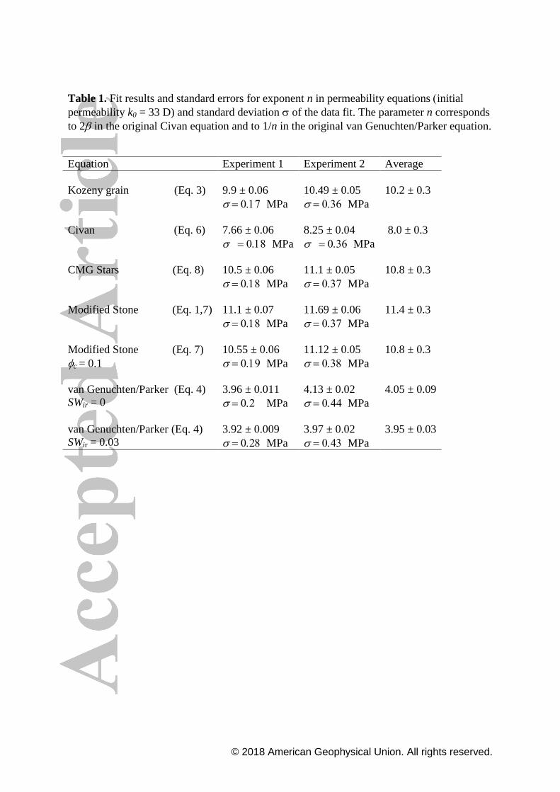
Table 1 lists the constrained values of the exponent n for the tested permeability
equations with their standard errors and the standard deviation of the corresponding fit of
the change in pressure difference. The reproducibility of the experimental procedure is
confirmed by the fact that the obtained exponents have comparable values for both
experiments. Standard deviations for the fit are almost identical for all equations, with the
exception of the van Genuchten/Parker equation. This holds true also after introducing an
irreducible water saturation SWir of 0.03. Hence, the shape of the simulated curve using the
van Genuchten/Parker equation is less suitable for describing the trend of the experimental
data, while all other equations result in similar fit qualities and are equally suitable for
describing the data.The fit for the modified Stone equation does not improve significantly
after introducing a nonzero value for the critical porosity c in order to represent a residual
gas saturation in the porous medium. We therefore hypothesize that c can be considered to
be zero for this experiment. This is a plausible assumption since the use of a vacuum pump
for the initial water saturation procedure should remove air in the sand matrix efficiently and
the subsequent pressurization to 12 MPa reduces the volume of possibly remaining gas
pockets by two orders of magnitude. With c =0, the modified Stone equation takes the form
of the U-Tokyo equation (Eq. 1). Supplements S3 and S4 include additional modeled curves
for different values of the exponent n.
The optimized curves for simulated changes in pressure difference versus
experimental data are presented in Figure 7. The error bars in the figure originate from the
fact that the experimental pressure differences had to be averaged over the duration of one
imaging run. Towards the end of the experiment, the pressure difference changed by several
MPa during the measurement time, resulting in larger error bars. The shape of the curves in
Figure 7 is similar except for the van Genuchten/Parker equation, which significantly
deviates from the trend in the data and rises too early. Figure 8 visualizes the equivalence of
the four suitable permeability equations for the constrained parameterizations (Tab. 1). The
curves differ mainly in the region of high gas hydrate saturations above SH = 0.75. At these
saturations, the permeability is extremely low (<110-16
m2) and the fluid flow in the sand
matrix is effectively blocked. Hence, the FEM simulations are not sensitive to locally
constrained further reductions in permeability. As a consequence, the permeability equations
are not well validated for very high gas hydrate saturations. The curves also show that the
reduction of the permeability is roughly exponential for the interval 0 <SH< 0.35, where it
drops by two orders of magnitude, and that the permeability decreases more strongly for
higher values of SH.
5 Sources of errors
The derived values for the exponent n are error-prone due to statistical and
experimental errors. Statistical errors are represented, for example, by the standard deviation
of the fits and the standard error of the optimized exponents, which are listed in Table 1.

© 2018 American Geophysical Union. All rights reserved.
Experimental errors and uncertainties include unaccounted-for signal losses (as discussed in
chapter 3.3) and the influence of the spatial and temporal resolution of the data acquisition.
The error arising from averaging of the pressure data over the time interval of the
imaging sequence is depicted by the error bars in Figure 7. It is caused by signal noise,
oscillations originating from the feedback loop of the sample cooling and the pressure rise
due to gas hydrate formation during the measurement time. The influence of these effects on
parameter n is in the order of 1% and can be neglected compared to other errors (see
Supplement S3 and S4).
The gas hydrate saturation in the sand sample increases during the duration of the
imaging experiment. As a consequence, the calculated gas hydrate saturations are time-
averaged values with unknown weightings. A comparison of the final MSSE image, which
was measured during gas hydrate formation, and the final MSME reference image, which
was measured after the formation had stopped shows that the uncertainty of the
experimentally derived gas hydrate saturations is in the range of a few percent of their
magnitude. This is the same range as the noise-related fluctuations within the images.
The spatial resolution of the images was chosen to be sufficiently large to average
over multiple grain diameters, but small enough to resolve variations in SH. This averaging
could mask true maximum values of SH, especially at the steep saturation gradient at the
bottom end of the gas hydrate patch. As shown in Figure 6, areas with large gas hydrate
saturations cover only part of the sample cross section. The fluid flow is diverted to regions
of lower, but much more homogeneous gas hydrate saturations and less steep saturation
gradients. The optimized permeability models indicate that the high saturation regions are
practically impermeable. In these regions, it does not matter if a coarse resolution results in
lower gas hydrate saturations as long as the derived saturation is high enough to also induce
an effective flow blockade. Because of their lower variability, the more homogeneous regions
do not require extremely high image resolutions. Therefore we do not expect to have large
errors due to resolution issues.
Relaxation of the NMR signal is enhanced in the proximity of sand grain surfaces
[Kleinberg et al., 2003]. Since the gas hydrate in a fully water-saturated porous medium is
expected to grow as pore-filling crystallites [Waite et al., 2009, Chaouachi et al., 2015],
residual water at grain surfaces might not contribute to the measured signal. This effect can
cause an overestimation of the calculated gas hydrate saturations. As a consequence, the true
values for n might be larger than the derived values.
Another source of error is the value of the initial permeability k0. It was measured
with a different setup and might deviate from the initial permeability of the actual samples.
Hence, we performed a second fit of the simulated data with k0 as an additional fitting
parameter. The results for the fitting parameters n and k0 and the standard deviation of the fits
are listed in Table 2. The measured value for k0 was 3.3×10⁻¹¹
m2. Fitted values range from
0.7×10⁻¹¹
m2 to 6.9×10
-11 m
2 except for the van Genuchten/Parker equation with SWir = 0,
which obtains a best fit for k0= 51×10-11
m2. However, the standard errors of the permeability
values are mostly larger than the values itself, indicating that the two fit parameters are not
independent from each other or that the order of magnitude for the permeability value is not
well constrained. This means, that k0 has to be provided by independent means to accurately
evaluate the data. Nevertheless, if the initial permeability is allowed to vary as a fitting
parameter, the measured value is reproduced within one order of magnitude and the results
for the exponents n only change within the range of their estimated experimental errors. This
evidence suggests that the values constrained for n are plausible and robust.
© 2018 American Geophysical Union. All rights reserved.
6 Discussion
6.1 Gas hydrate growth habits
The primary applications for permeability equations predicting the effect of gas
hydrates forming in the sediment pore space are gas production simulations of gas hydrate
reservoirs and simulations of fluid flow dynamics in gas hydrate / seep systems. Thus, it is
important that gas hydrate sediments used in laboratory studies resemble the relevant natural
properties as closely as possible. Typically, artificial CH4 hydrates are precipitated from a
limited amount of water in partially water-saturated sediments exposed to a high-pressure
methane atmosphere, because this is the most convenient method. One advantage of this
procedure is the almost immediate start of gas hydrate nucleation due to the excess supply of
gas molecules in comparison to the method of a gas-saturated solution where the stochastic
onset of gas hydrate nucleation may take several days to weeks. Another advantage of the
partial saturation method is that the final gas hydrate saturation can be controlled by varying
the amount of water in the sediment. However, X-Ray CT data published by Kneafsey et al.
[2011] and Seol and Kneafsey [2011] question the common belief that the partial water-
saturation method yields a homogeneous gas hydrate distribution in the sample. Their gas
hydrate saturation maps demonstrate distinct spatial inhomogeneities. We have evidence
from MRI data [Kossel et al., 2013b] that the degree of homogeneity depends on the initial
water distribution in the sample and on the completeness of the water consumption in the
course of gas hydrate formation. The water is evenly distributed only if the capillary forces
are larger than the gravitational force. If the influence of gravitation leads to an accumulation
of water at the bottom of the sample, gas hydrate saturation, too, will be higher at the bottom.
A fast pressurization of the sample can also lead to a redistribution of the water phase. Even
for homogeneous initial water distributions, gas hydrate formation does not occur
simultaneously across the sample. The transformation of gas and water into gas hydrates is
accelerated in some parts of the volume, probably because of local oversaturation of gas in
the liquid phase. Only for a complete conversion of water to hydrate does the gas hydrate
distribution correspond to the initial water distribution. Therefore, a spatially resolved
monitoring of the gas hydrate formation in sediment matrices and a characterization of the
final distribution is equally mandatory for both the partial water-saturation method as well as
the gas-saturated solution method. If the occurrence of inhomogeneities is confirmed, data
evaluation has to be performed for a full three-dimensional representation of the sample. This
is always recommended for gas hydrate formation from gas-saturated solution because gas
hydrate saturations will vary in space and locally also in time, as our experiments have
demonstrated. However, it needs to be stressed that this is the dominant formation
mechanism of natural marine gas hydrates, which preferentially show a pore-filling growth
habit [Waite et al., 2009]. Hence, gas hydrate formation from gas-saturated solution is better
suited to mimic natural gas hydrate properties.
Water in a partially water-saturated sediment sample is wetting the sediment grains,
i.e. forming a thin film of water around the grains as well as menisci between neighboring
grains. Consequently, gas hydrates can only form from these water films leading to a grain-
coating and pore throat-clogging growth habit, whereas gas hydrates in a fully water-
saturated sand matrix form preferentially in the pore centers [Tohidi et al., 2001; Jin et al.,
2012, Chaouachi et al., 2015]. Increasing the water saturation in a partially water-saturated
medium is believed to induce a transition from grain-coating gas hydrates to pore-filling gas
hydrates when the water film around the grains increases in thickness [Delli and Grosic,
2013]. It is plausible, that the flow obstruction resulting from both methods is different: The
pressure in our experiments raises little for low to moderate gas hydrate saturations and
© 2018 American Geophysical Union. All rights reserved.
increases strongly at large gas hydrate saturations. This behavior is typical for gas hydrates
that grow predominantly in the pore centers and fill the pore throats only at high saturations.
Grain-coating gas hydrates will clog up pore throats quickly and thus, reduce permeability
more effectively already at lower gas hydrate saturations compared to the pore-filling growth
habit. Therefore, grain-coating growth behavior at low water saturation is expected to result
in even higher values of n than those determined in our experiments.
6.2 Permeability as a function of gas hydrate saturation
Four of the five tested permeability equations show the capability to reproduce our
experimental data equally well: The pore-filling type Kozeny grain equation, the Civan
equation, the CMG Stars equation and the modified Stone equation including its simplified
version, the U-Tokyo equation. One similarity of the suitable equations is the factor (1-SH)n.
The less suitable van Genuchten/Parker equation is the only one that does not include this
specific term. This finding indicates, that (1-SH)n is the governing factor describing the
permeability behavior, and the most basic permeability equation would be k = k0(1-SH)n,
which is the modified Stone equation for a critical porosity of ϕc=0 (Eq.1). Reducing a model
equation to its mathematically least complex form is also always beneficial in numerical
simulations. Therefore, we recommend this simple equation to be used in numerical models
of single phase water flow in gas hydrate bearing sediments. In contrast to the Kozeny grain
equation, the Civan, CMG Stars and modified Stone equations have the advantage, that their
formalism also includes equations for multiphase flow gas/water permeabilities. Therefore,
these equations are preferred for simulations of complex multiphase flow problems.
However, gas permeability equations and multiphase flow equations have not been evaluated
and tested explicitly within the scope of our study. Hence, we cannot make solid statements
about the reliability of our optimized equations in the context of multiphase flow.
Our result for the exponent of the modified Stone equation with fc= 0, n=11.4, is
larger than most published values. The majority of the published results for n range from 2.5
to 10 [Minagawa et al., 2005; Liang et al., 2011; Konno et al., 2013; Delli and Grosic, 2014;
Li et al., 2014] with the values either being about 3 or about 9. An exception is the work of Li
et al. [2013] who report a value of n=38 and the results of Masuda et al. [2005], who derived
n=14. In contrast to these studies, we evaluated time dependent 3-D maps of the gas hydrate
saturation. We could identify transport pathways with lower than average gas hydrate
saturations. A smaller SH requires a larger n to yield the same permeability reduction.
Therefore, it is plausible that our larger result for n is a consequence of our more elaborate
and accurate data evaluation procedure, which is not reduced to averaged gas hydrate
saturations of the entire sample volume. The discussion of errors in section 5 concludes that
the uncertainty of our result is expected to be in the order of 10% of its value. Consequently,
our value for n remains still larger than most previous estimates even if possible errors are
considered. In gas hydrate reservoir simulations, generally relatively low exponent values of
n =2-5 have been used with the tested permeability equations so far (e.g., [Anderson et al,
2011; Kurihara et al., 2011; Moridis et al., 2011; Schoderbek et al, 2013; Mahabadi and
Jang, 2014; Reagan et al., 2015]). As a consequence, simulated gas production rates might be
overestimated or induced permeability errors have been compensated by twitching other
unknown model parameterizations during history matching of field trial production data.
Hence, using our optimized permeability equations may help improving gas production
simulations as well as understanding the effects of true spatial inhomogeneities in the gas
hydrate distribution in reservoirs or in laboratory experiments. This, of course, requires that
spatial inhomogeneities are included in the simulations and the resolution of the model grid is
sufficiently high. Since this is not always feasible, an alternative option would therefore be

© 2018 American Geophysical Union. All rights reserved.
the introduction of effective gas hydrate saturations that are based on typical gas hydrate
saturation distributions in natural sediments. The value of the effective gas hydrate saturation
would mainly be determined by low-saturation flow paths and is expected to be smaller than
the average gas hydrate saturation. This smaller value would counteract the effect of the
supposedly more accurate larger exponents in the permeability equation to some extent.
Experimental results and model parametrizations presented in this study can be used to derive
effective permeability models including the knowledge available for a particular setting and
help to evaluate uncertainties in model upscaling and reservoir prediction. Moreover, our
optimized permeability equations can also help in interpreting and predicting the patchiness
of natural gas hydrate accumulations, the formation and evolution of fluid migration
pathways, such as seismic pipes and chimneys, in the gas hydrate stability zone and of cold
seeps as their surface expressions. These studies have rarely applied any feedback of gas
hydrates directly on permeability.
7 Conclusions
We have designed an experimental set-up that allowed us to determine the water
permeability in CH4-hydrate-bearing quartz sand with known gas hydrate saturation and
distribution. To avoid the less prevalent grain-coating growth habit, gas hydrates were formed
from a methane-saturated aqueous solution. Three-dimensional time-dependent maps of gas
hydrate saturations were constructed from MRIs of the sample volume and fed into FEM
simulations for a detailed and elaborate evaluation of the occurring flow obstructions. It was
shown, that the gas hydrate formation was spatially inhomogeneous and required a full 3-D
modeling of the flow field. We compared five widely-used permeability equations for their
capability to reproduce the experimental results: the pore-filling Kozeny grain equation, the
van Genuchten/Parker equation, the Civan equation, the modified Stone equation and the
CMG Stars equation. All equations of the general form k ~ k0 (1-SH)n with n as fitting
parameter were able to reproduce the experimental data equally well. The van
Genuchten/Parker equation, which does not contain this specific term, produced an inferior
result in matching the experimental data. Our findings indicate that (1-SH)n is the governing
factor in the suitable permeability equations, and that the most basic permeability equation
for single-phase water flow through gas hydrate bearing sand is k = k0 (1-SH)n. For this
specific equation, an exponent n = 11.4 ± 0.3 was determined. Since small gas hydrate
saturations were barely present in the sample and high gas hydrate saturations resulted in an
efficient blockage of the water flow, the derived parameters are best validated for medium
gas hydrate saturations of 0.3-0.7. We derived higher equation exponents than most other
studies, which can be explained by our more detailed knowledge of the spatial and temporal
distribution of the gas hydrate saturation. We could identify pathways with smaller than
average gas hydrate saturations that dominate the transport properties. Explicitly including
those pathways into the data evaluation instead of using average gas hydrate saturations
results in the need for higher values of n in order to derive the same flow resistance.
Acknowledgements
Data will be made available in the PANGEA open access data library (details will be
added at acceptance of manuscript). This research was funded by the German Ministry of
Economy (BMWi) through the SUGAR project (grant No. 03SX320A) and by the European
Community’s 7th Framework Program (FP7/2007-2013) through the ECO2 project (grant
agreement no. 265847).

© 2018 American Geophysical Union. All rights reserved.
References
Ahn, T., J. Lee, D.-G. Huh, and J. M. Kang (2005), Experimental study on two-phase flow in
artificial hydrate-bearing sediments, Geosystem Engineering, 8(4), 101-104,
doi:10.1080/12269328.2005.10541244.
Anderson, B. J., M. Kurihara, M. D. White, G. J. Moridis, S. J. Wilson, M. Pooladi-Darvish,
M. Gaddipati, Y. Masuda, T. S. Collett, R. B. Hunter, H. Narita, K. Rose and R.
Boswell, (2011), Regional long-term production modeling from a single well test,
Mount Elbert Gas Hydrate Stratigraphic Test Well, Alaska North Slope, Mar. Pet.
Geol., 28(2), 493-501, doi:10.1016/j.marpetgeo.2010.01.015.
Bai, Y., Q. Li, X. Li, and Y. Du (2008), The simulation of nature gas production from ocean
gas hydrate reservoir by depressurization, Science in China Series E-Technological
Sciences, 51(8), 1272-1282, doi:10.1007/s11431-008-0146-1.
Buffett, B., and D. Archer (2004), Global inventory of methane clathrate: Sensitivity to
changes in the deep ocean, Earth and Planetary Science Letters, 227(3-4), 185-199,
doi:10.1016/j.epsl.2004.09.005.
Callaghan, P.T. (1993), Principles of Nuclear Magnetic Resonance Microscopy, Oxford
University Press, Oxford, doi:10.1002/mrc.1260330417
Carman, P. C. (1937), Fluid flow through granular beds, Transactions Institution of Chemical
Engineers, 15, 150-166.
Chaouachi, M., A. Falenty, K. Sell, F. Enzmann, M. Kersten, D. Haberthuer, and W. F. Kuhs
(2015), Microstructural evolution of gas hydrates in sedimentary matrices observed
with synchrotron X-ray computed tomographic microscopy, Geochemistry
Geophysics Geosystems, 16(6), 1711-1722, doi:10.1002/2015gc005811.
Civan, F. (2001), Scale effect on porosity and permeability: Kinetics, model, and correlation,
AIChE Journal, 47(2), 271-287, doi:10.1002/aic.690470206.
CMG (2009), STARS advanced process and thermal reservoir simulator (user’s guide),
Calgary, Canada.
Cyranoski, D. (2013), Japanese test coaxes fire from ice, Nature, 496(7446), 409-409.
Dallimore, S. R., and T. S. Collett (Eds.) (2005), Scientific results from the Mallik 2002 gas
hydrate production research well program, Mackenzie Delta, Northwest Territories,
Canada, Geological Survey of Canada Bulletin, Ottawa, Canada.
Dallimore, S. R., K. Yamamoto, J. F. Wright, and G. Bellefleur (Eds.) (2012), Scientific
results from the JOGMEC/NRCan/Aurora Mallik 2007-2008 gas hydrate production
research well program, Mackenzie Delta, Northwest Territories, Canada, Geological
Survey of Canada Bulletin, Ottawa, Canada.
Delli, M. L., and J. L. H. Grozic (2013), Prediction performance of permeability models in
gas-hydrate-bearing sands, Spe J., 18(2), 274-284, doi:10.2118/149508-PA.
Delli, M. L., and J. L. H. Grozic (2014), Experimental determination of permeability of
porous media in the presence of gas hydrates, J. Pet. Sci. Eng., 120, 1-9,
doi:10.1016/j.petrol.2014.05.011.
Duan, Z. H., and S. D. Mao (2006), A thermodynamic model for calculating methane
solubility, density and gas phase composition of methane-bearing aqueous fluids from
273 to 523 K and from 1 to 2000 bar, Geochimica et Cosmochimica Acta, 70(13),
3369-3386, doi:10.1016/j.gca.2006.03.018.
© 2018 American Geophysical Union. All rights reserved.
Jin, Y., J. Hayashi, J. Nagao, K. Suzuki, H. Minagawa, T. Ebinuma, and H. Narita (2007),
New method of assessing absolute permeability of natural methane hydrate sediments
by microfocus X-ray computed tomography, Jpn. J. Appl. Phys. Part 1 - Regul. Pap.
Brief Commun. Rev. Pap., 46(5A), 3159-3162, doi:10.1143/jjap.46.3159.
Jin, Y., Y. Konno, and J. Nagao (2012), Growth of methane clathrate hydrates in porous
media, Energy & Fuels, 26(4), 2242-2247, doi:10.1021/ef3001357.
Johnson, A., S. Patil, and A. Dandekar (2011), Experimental investigation of gas-water
relative permeability for gas-hydrate-bearing sediments from the Mount Elbert gas
hydrate stratigraphic test well, Alaska North Slope, Mar. Pet. Geol., 28(2), 419-426,
doi:10.1016/j.marpetgeo.2009.10.013.
Kleinberg, R. L., C. Flaum, D. D. Griffin, P. G. Brewer, G. E. Malby, E. T. Peltzer, and J. P.
Yesinowski (2003), Deep sea NMR: Methane hydrate growth habit in porous media
and its relationship to hydraulic permeability, deposit accumulation, and submarine
slope stability, J. Geophys. Res.-Solid Earth, 108(B10), 17,
doi:10.1029/2003jb002389.
Kneafsey, T. J., Y. Seol, A. Gupta, and L. Tomutsa (2011), Permeability of laboratory-
formed methane-hydrate-bearing sand: Measurements and observations using X-Ray
computed tomography, Spe J., 16(1), 78-94, doi:10.2118/139525-PA.
Konno, Y., Y. Jin, T. Uchiumi, and J. Nagao (2013), Multiple-pressure-tapped core holder
combined with X-ray computed tomography scanning for gas-water permeability
measurements of methane-hydrate-bearing sediments, Rev. Sci. Instrum., 84(6), 5,
doi:10.1063/1.4811379.
Kossel, E., N. Bigalke, E. Pinero, and M. Haeckel (2013a), The SUGAR Toolbox : A library
of numerical algorithms and data for modelling of gas hydrate systems and marine
environments, GEOMAR Report 8, GEOMAR Helmholtz-Zentrum für
Ozeanforschung Kiel, Kiel, Germany, doi:10.3289/GEOMAR_REP_NS_8_2013.
Kossel, E., C. Deusner, N. Bigalke, and M. Haeckel (2013b), Magnetic resonance imaging of
gas hydrate formation and conversion at sub-seafloor conditions, Diffusion
Fundamentals, 18(15), 1-4.
Kozeny, J. (1927), Über kapillare Leitung des Wassers im Boden, Sitzungsberichte
Akademie der Wissenschaften Wien, 136, 271-306.
Kurihara, M., H. Ouchi, T. Inoue, T. Yonezawa, Y. Masuda, S. R. Dallimore, and T. S.
Collett (2005), Analysis of the JAPEX/JNOC/GSC et al. Mallik 5L-38 gas hydrate
thermal-production test through numerical simulation, Geological Survey of Canada
Bulletin, 585, 1-20.
Kurihara, M., A. Sato, K. Funatsu, H. Ouchi, Y. Masuda, H. Narita, and T. S. Collett (2011),
Analysis of formation pressure test results in the Mount Elbert methane hydrate
reservoir through numerical simulation, Mar. Pet. Geol., 28(2), 502-516,
doi:10.1016/j.marpetgeo.2010.01.007.
Li, G., G. J. Moridis, K. N. Zhang, and X. S. Li (2010), Evaluation of gas production
potential from marine gas hydrate deposits in Shenhu Area of South China Sea,
Energy & Fuels, 24, 6018-6033, doi:10.1021/ef100930m.
Li, B., X. S. Li, G. Li, J. L. Jia, and J. C. Feng (2013), Measurements of water permeability in
unconsolidated porous media with methane hydrate formation, Energies, 6(7), 3622-
3636, doi:10.3390/en6073622.
© 2018 American Geophysical Union. All rights reserved.
Li, C. H., Q. Zhao, H. J. Xu, K. Feng, and X. W. Liu (2014), Relation between relative
permeability and hydrate saturation in Shenhu area, South China Sea, Appl. Geophys.,
11(2), 207-214, doi:10.1007/s11770-014-0432-6.
Liang, H., Y. Song, and Y. Liu (2011), The measurement of permeability of porous media
with methane hydrate, Pet. Sci. Technol., 29(1), 78-87, doi:
10.1080/10916460903096871.
Luo, M., A. W. Dale, L. Haffert, M. Haeckel, S. Koch, G. Crutchley, H. De Stigter, D. Chen,
and J. Greinert (2016), A quantitative assessment of methane cycling in Hikurangi
Margin sediments (New Zealand) using geophysical imaging and biogeochemical
modeling, Geochemistry, Geophysics, Geosystems.
Mahabadi, N., and J. Jang (2014), Relative water and gas permeability for gas production
from hydrate-bearing sediments, Geochemistry Geophysics Geosystems, 15(6), 2346-
2353, doi:10.1002/2014gc005331.
Masuda, Y., S. Naganawa, S. Ando, and K. Sato (1997), Numerical calculations of gas
hydrate production performance from reservoirs containing natural gas hydrates,
paper presented at Western Regional Meeting, Society of Petroleum Engineers, Long
Beach, California.
Masuda, Y., Y. Konno, M. Kurihara, H. Ouchi, Y. Kamat, T. Ebinuma, H. Narita (2005),
Validation study of numerical simulator predicting gas production performance from
sediments containing methane hydrates, paper presented at 5th International
Conference on Gas Hydrates (ICGH 2005), Trondheim, Norway.
Minagawa, H., R. Ohmura, Y. Kamata, T. Ebinuma, and H. Narita (2005), Water
permeability measurements of gas hydrate-bearing sediments, paper presented at the
5th International Conference on Gas Hydrates, Trondheim, Norway.
Moridis, G. J. (2004), Numerical studies of gas production from class 2 and class 3 hydrate
accumulations at the Mallik site, Mackenzie Delta, Canada, SPE Reserv. Eval. Eng.,
7(3), 175-183, doi:10.2118/88039-PA.
Moridis, G. J., T. S. Collett, S. R. Dallimore, T. Inoue, and T. Mroz (2005), Analysis and
interpretation of the thermal test of gas hydrate dissociation in the JAPEX/JNOC/GSC
et al. Mallik 5L-38 gas hydrate production research well, Geological Survey of
Canada Bulletin, 585, 1-21.
Moridis, G. J., and E. D. Sloan (2007), Gas production potential of disperse low-saturation
hydrate accumulations in oceanic sediments, Energy Conv. Manag., 48(6), 1834-
1849, doi:10.1016/j.enconman.2007.01.023.
Moridis, G. J., S. Silpngarmlert, M. T. Reagan, T. Collett, and K. Zhang (2011), Gas
production from a cold, stratigraphically-bounded gas hydrate deposit at the Mount
Elbert Gas Hydrate Stratigraphic Test Well, Alaska North Slope: Implications of
uncertainties, Mar. Pet. Geol., 28(2), 517-534, doi:10.1016/j.marpetgeo.2010.01.005.
Mualem, Y. (1976), A new model for predicting the hydraulic conductivity of unsaturated
porous media, Water Resources Research, 12(3), 513-522.
Parker, J. C., R. J. Lenhard, and T. Kuppusamy (1987), A parametric model for constitutive
properties governing multiphase flow in porous media, Water Resources Research,
23(4), 618-624, doi:10.1029/WR023i004p00618.
© 2018 American Geophysical Union. All rights reserved.
Pinero, E., M. Marquardt, C. Hensen, M. Haeckel, and K. Wallmann (2013), Estimation of
the global inventory of methane hydrates in marine sediments using transfer
functions, Biogeosciences, 10(2), 959-975, doi:10.5194/bg-10-959-2013.
Pinero, E., C. Hensen, M. Haeckel, W. Rottke, T. Fuchs, and K. Wallmann (2016), 3-D
numerical modelling of methane hydrate accumulations using PetroMod, Mar. Pet.
Geol., 71, 288-295, doi:10.1016/j.marpetgeo.2015.12.019.
Reagan, M.T., G.J. Moridis, J.N. Johnson, L. Pan, C.M. Freeman, L. Pan, K.L. Boyle, N.D.
Keen, J. Husebo (2015), Field-scale simulation of production from oceanic gas
hydrate deposits, Transport in Porous Media, 108, 151-169, doi:10.1007/s11242-014-
0330-7.
Sakamoto, Y., T. Komai, K. Myazaki, N. Tenma, T. Yamaguchi, and G. Zyvoloski (2010),
Laboratory-scale experiments of methane hydrate dissociation process in a porous
media and numerical study for the estimation of permeability in methane hydrate
reservoir, Journal of Thermodynamics, 2010, 1-13, doi:10.1155/2010/452326.
Schoderbek, D., H. Farrell, K. Hester, J. Howard, K. Raterman, S. Silpngarmlert, K. L.
Martin, B. Smith, and P. Klein (2013), ConocoPhillips gas hydrate production test
final technical report, United States Department of Energy, available online at
http://www.netl.doe.gov.
Seol, Y., and T. J. Kneafsey (2011), Methane hydrate induced permeability modification for
multiphase flow in unsaturated porous media, J. Geophys. Res.-Solid Earth, 116, 1-
15, doi:10.1029/2010jb008040.
Sloan, E. D. (2003), Fundamental principles and applications of natural gas hydrates, Nature,
426(6964), 353-359, doi:10.1038/nature02135.
Sloan, E. D., and C. A. Koh (2008), Clathrate hydrates of natural gases, 3rd ed., CRC Press,
New York.
Spangenberg, E. (2001), Modeling of the influence of gas hydrate content on the electrical
properties of porous sediments, J. Geophys. Res. Solid Earth, 106(B4), 6535-6548,
doi:10.1029/2000jb900434.
Stone, H. L. (1970), Probability model for estimating three-phase relative permeability,
Journal of Petroleum Technology, 22(2), 214-218, doi:10.2118/2116-PA.
Sun, X. F., and K. K. Mohanty (2006), Kinetic simulation of methane hydrate formation and
dissociation in porous media, Chemical Engineering Science, 61(11), 3476-3495,
doi:10.1016/j.ces.2005.12.017.
Tishchenko, P., C. Hensen, K. Wallmann, and C. S. Wong (2005), Calculation of the stability
and solubility of methane hydrate in seawater, Chemical Geology, 219(1-4), 37-52,
doi:10.1016/j.chemgeo.2005.02.008.
Tohidi, B., R. Anderson, M. B. Clennell, R. W. Burgass, and A. B. Biderkab (2001), Visual
observation of gas-hydrate formation and dissociation in synthetic porous media by
means of glass micromodels, Geology, 29(9), 867-870,
doi:10.1130/00917613(2001)029<0867:vooghf>2.0.co;2.
U.S. Geological Survey Gas Hydrates Project (2014), Database of worldwide gas hydrates,
available online at https://woodshole.er.usgs.gov/project-
pages/hydrates/database.html
© 2018 American Geophysical Union. All rights reserved.
van Genuchten, M. T. (1980), A closed-form equation for predicting the hydraulic
conductivity of unsaturated soils, Soil Science Society of America Journal, 44(5),
892-898.
Waite, W. F., J. C. Santamarina, D.D. Cortes, B. Dugan. D. N. Espinoza, J. Germaine, J.
Jang, J. W. Jung, T. J. Kneafsey, H. Shin, K. Soga, W. J. Winters (2009), Physical
properties of hydrate-bearing sediments, Reviews of Geophysics, 47,
doi:Rg400310.1029/2008rg000279.
Wallmann, K., E. Pinero, E. Burwicz, M. Haeckel, C. Hensen, A. Dale, and L. Rüpke (2012),
The global inventory of methane hydrate in marine sediments: A theoretical approach,
Energies, 5(7), 2449-2498, doi:10.3390/en5072449.
Weishaupt D., V. D. Köchli and B Marincek (2008), How does MRI work?, Springer Verlag,
Berlin, Heidelberg, doi:10.1007/978-3-540-37845-7
Wilder, J. W., G. J. Moridis, S. J. Wilson, M. Kurihara, M. D. White, Y. Masuda, B. J.
Anderson, T. S. Collett, R. B. Hunter, H. Narita, M. Pooladi-Darvish, K. Rose and R.
Boswell (2008), An international effort to compare gas hydrate reservoir simulators,
paper presented at 6th International Conference on Gas Hydrates (ICGH 2008),
Vancouver, British Columbia, Canada, July 6-10, 2008.
© 2018 American Geophysical Union. All rights reserved.
Table 1. Fit results and standard errors for exponent n in permeability equations initial
permeability k0 = 33 D) and standard deviation of the data fit. The parameter n corresponds
to 2 in the original Civan equation and to 1/n in the original van Genuchten/Parker equation.
Equation Experiment 1 Experiment 2 Average
Kozeny grain (Eq. 3) 9.9 ± 0.06 10.49 ± 0.05 10.2 ± 0.3
MPa MPa
Civan (Eq. 6) 7.66 ± 0.06 8.25 ± 0.04 8.0 ± 0.3
MPa MPa
CMG Stars (Eq. 8) 10.5 ± 0.06 11.1 ± 0.05 10.8 ± 0.3
MPa MPa
Modified Stone (Eq. 1,7) 11.1 ± 0.07 11.69 ± 0.06 11.4 ± 0.3
MPa MPa
Modified Stone (Eq. 7) 10.55 ± 0.06 11.12 ± 0.05 10.8 ± 0.3
c = 0.1
MPa MPa
van Genuchten/Parker (Eq. 4) 3.96 ± 0.011 4.13 ± 0.02 4.05 ± 0.09
SWir = 0 MPa MPa
van Genuchten/Parker (Eq. 4) 3.92 ± 0.009 3.97 ± 0.02 3.95 ± 0.03
SWir = 0.03 MPa MPa
© 2018 American Geophysical Union. All rights reserved.
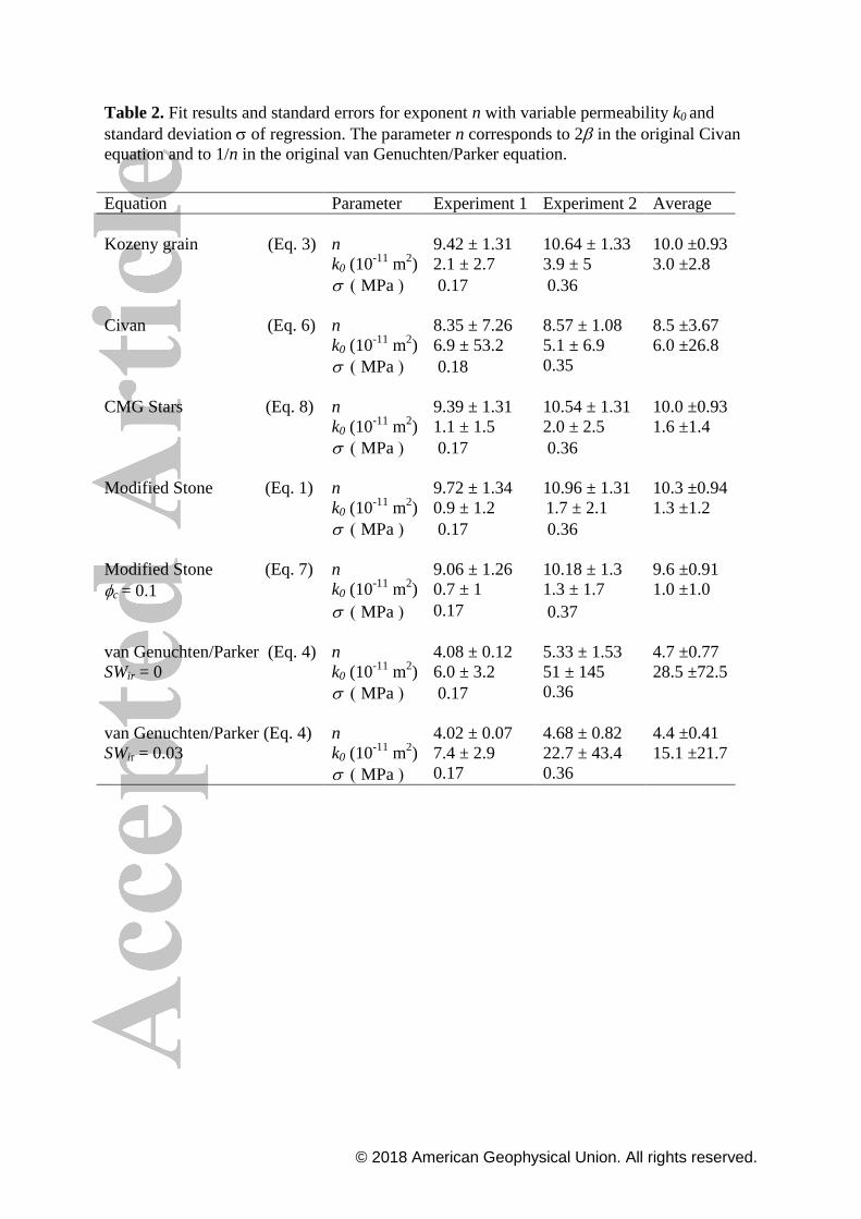
Table 2. Fit results and standard errors for exponent n with variable permeability k0 and
standard deviation of regression. The parameter n corresponds to 2 in the original Civan
equation and to 1/n in the original van Genuchten/Parker equation.
Equation Parameter Experiment 1 Experiment 2 Average
Kozeny grain (Eq. 3) n 9.42 ± 1.31 10.64 ± 1.33 10.0 ±0.93
k0 (10-11
m2) 2.1 ± 2.7 3.9 ± 5 3.0 ±2.8
MPa 0.17 0.36
Civan (Eq. 6) n 8.35 ± 7.26 8.57 ± 1.08 8.5 ±3.67
k0 (10-11
m2) 6.9 ± 53.2 5.1 ± 6.9 6.0 ±26.8
MPa 0.18 0.35
CMG Stars (Eq. 8) n 9.39 ± 1.31 10.54 ± 1.31 10.0 ±0.93
k0 (10-11
m2) 1.1 ± 1.5 2.0 ± 2.5 1.6 ±1.4
MPa 0.17 0.36
Modified Stone (Eq. 1) n 9.72 ± 1.34 10.96 ± 1.31 10.3 ±0.94
k0 (10-11
m2) 0.9 ± 1.2 1.7 ± 2.1 1.3 ±1.2
MPa 0.17 0.36
Modified Stone (Eq. 7) n 9.06 ± 1.26 10.18 ± 1.3 9.6 ±0.91
c = 0.1 k0 (10-11
m2) 0.7 ± 1 1.3 ± 1.7 1.0 ±1.0
MPa 0.17 0.37
van Genuchten/Parker (Eq. 4) n 4.08 ± 0.12 5.33 ± 1.53 4.7 ±0.77
SWir = 0 k0 (10-11
m2) 6.0 ± 3.2 51 ± 145 28.5 ±72.5
MPa 0.17 0.36
van Genuchten/Parker (Eq. 4) n 4.02 ± 0.07 4.68 ± 0.82 4.4 ±0.41
SWir = 0.03 k0 (10-11
m2) 7.4 ± 2.9 22.7 ± 43.4 15.1 ±21.7
MPa 0.17 0.36
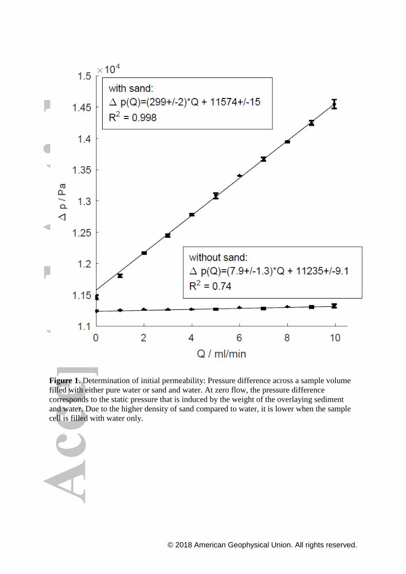
© 2018 American Geophysical Union. All rights reserved.
Figure 1. Determination of initial permeability: Pressure difference across a sample volume
filled with either pure water or sand and water. At zero flow, the pressure difference
corresponds to the static pressure that is induced by the weight of the overlaying sediment
and water. Due to the higher density of sand compared to water, it is lower when the sample
cell is filled with water only.
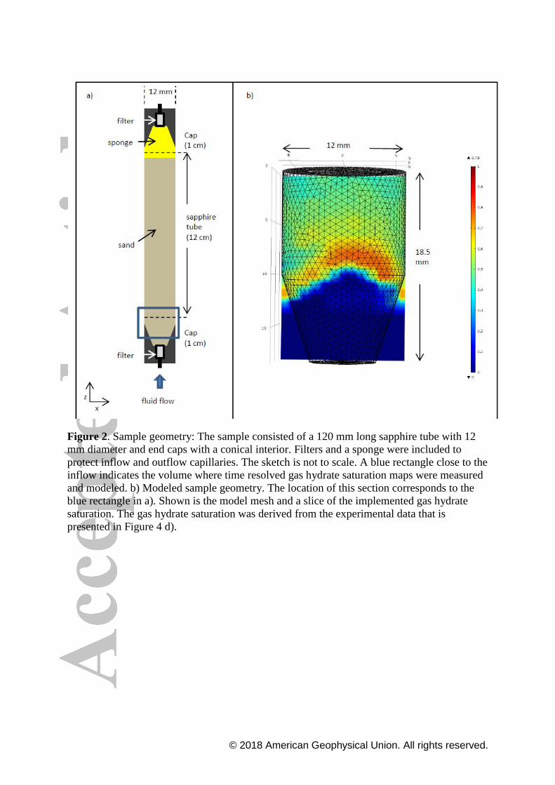
© 2018 American Geophysical Union. All rights reserved.
Figure 2. Sample geometry: The sample consisted of a 120 mm long sapphire tube with 12
mm diameter and end caps with a conical interior. Filters and a sponge were included to
protect inflow and outflow capillaries. The sketch is not to scale. A blue rectangle close to the
inflow indicates the volume where time resolved gas hydrate saturation maps were measured
and modeled. b) Modeled sample geometry. The location of this section corresponds to the
blue rectangle in a). Shown is the model mesh and a slice of the implemented gas hydrate
saturation. The gas hydrate saturation was derived from the experimental data that is
presented in Figure 4 d).

© 2018 American Geophysical Union. All rights reserved.
Figure 3. Measured pressure difference between the pressure sensors downstream and
upstream of the sample cell during gas hydrate formation in a quartz sand matrix: a)
Experiment 1, b) Experiment 2. The experiments were automatically terminated when the
upstream pressure exceeded 15 MPa.
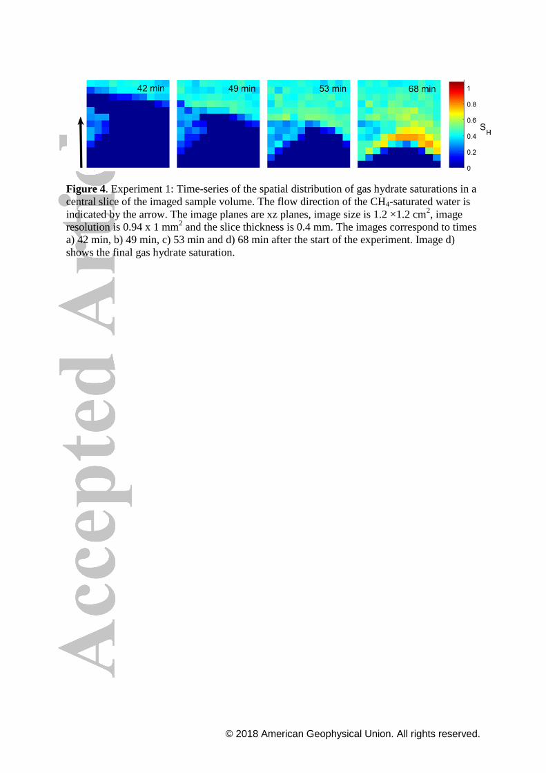
© 2018 American Geophysical Union. All rights reserved.
Figure 4. Experiment 1: Time-series of the spatial distribution of gas hydrate saturations in a
central slice of the imaged sample volume. The flow direction of the CH4-saturated water is
indicated by the arrow. The image planes are xz planes, image size is 1.2 ×1.2 cm2, image
resolution is 0.94 x 1 mm2 and the slice thickness is 0.4 mm. The images correspond to times
a) 42 min, b) 49 min, c) 53 min and d) 68 min after the start of the experiment. Image d)
shows the final gas hydrate saturation.

© 2018 American Geophysical Union. All rights reserved.
Figure 5. Experiment 2: Time-series of the spatial distribution of gas hydrate saturations in a
central slice of the imaged sample volume. The flow direction of the CH4-saturated water is
indicated by the arrow. The image planes are yz planes, image size is 1.2 ×1.2 cm2,image
resolution is 0.47 x 0.4 mm2and the slice thickness is 1 mm. The images correspond to times
a) 214 min, b) 223 min, c) 233 min and d) 244 min after the start of the experiment. Image d)
shows the final gas hydrate saturation.

© 2018 American Geophysical Union. All rights reserved.
Figure 6. Projected planes of maximum gas hydrate saturation in the xy plane perpendicular
to the flow direction at the end of a) Experiment 1 and b) Experiment 2. The image size is 1.2
×1.2 cm2 and image resolution is 0.04 x 0.1 cm
2. Experiments were aborted at the same final
upstream pressure of 15 MPa, but had different downstream pressures. Thus, the final
pressure difference was higher in Experiment 2, resulting in higher gas hydrate saturations.
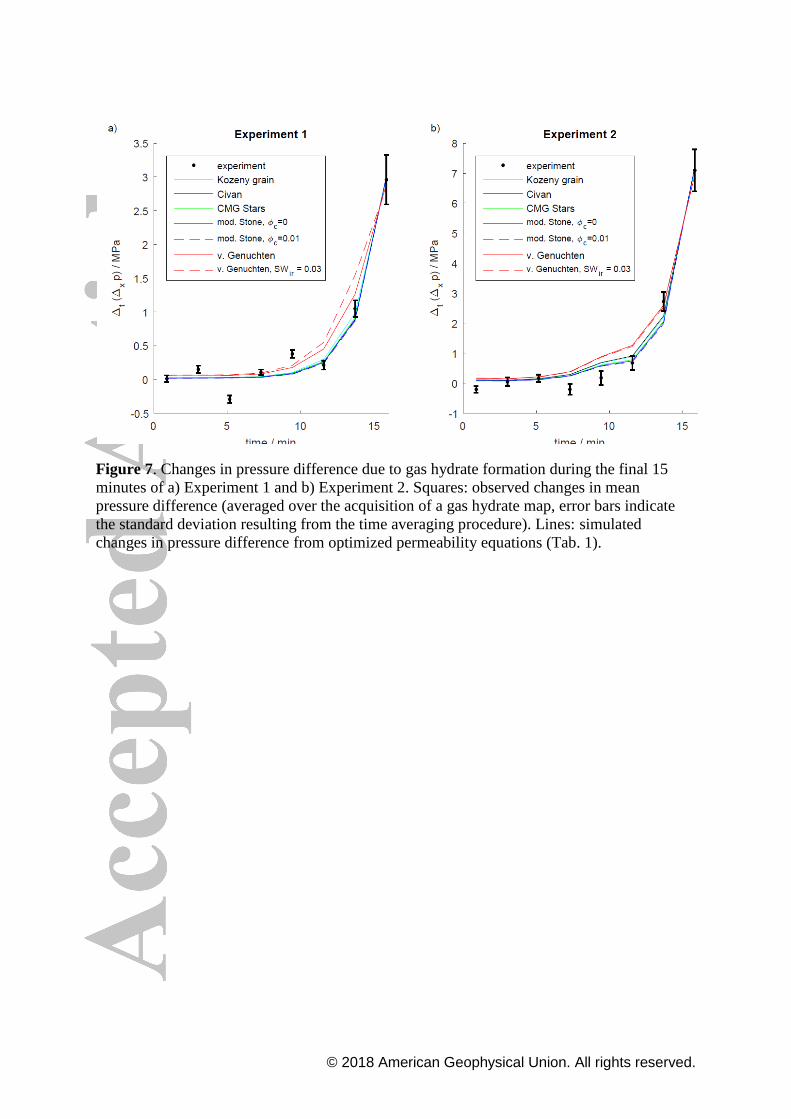
© 2018 American Geophysical Union. All rights reserved.
Figure 7. Changes in pressure difference due to gas hydrate formation during the final 15
minutes of a) Experiment 1 and b) Experiment 2. Squares: observed changes in mean
pressure difference (averaged over the acquisition of a gas hydrate map, error bars indicate
the standard deviation resulting from the time averaging procedure). Lines: simulated
changes in pressure difference from optimized permeability equations (Tab. 1).

© 2018 American Geophysical Union. All rights reserved.
Figure 8. Water permeability as a function of gas hydrate saturation. The curves for the
different permeability equations were calculated using the parameter values listed in Table 1.
The modified Stone equation is used with c=0 and the van Genuchten equation with SirW =
0.