Instructions for use

Title Depth dependence and exponential models of permeability in alluvial-fan gravel deposits

Author(s) Sakata, Yoshitaka; Ikeda, Ryuji

Citation Hydrogeology Journal, 21(4): 773-786

Issue Date 2013-06

Doc URL http://hdl.handle.net/2115/56468

Rights The final publication is available at link.springer.com

Type article (author version)

File Information Sakata (2013) Depth-dependence of permeability-1.pdf

Hokkaido University Collection of Scholarly and Academic Papers : HUSCAP

1

Depth dependence and exponential models of permeability in alluvial-fan gravel deposits Yoshitaka SAKATA1・Ryuji IKEDA2 1. First affiliation: Division of Earth and Planetary Dynamics, Graduate School of Science, Hokkaido University North-10, West-8, Kita-ku, Sapporo, Hokkaido 060-0810, Japan Second affiliation: Geotechnical Department, Division of Environmental Engineering, Docon Co., Ltd. Atsubetsu-chuo-1-5, Atsubetsu-ku, Sapporo, Hokkaido 004-8585, Japan E-mail: yoshitaka_sakata@mail.sci.hokudai.ac.jp Telephone/Fax: +81-11-706-2756 Affiliation: Division of Earth and Planetary Dynamics, Faculty of Science, Hokkaido University Address: North-10, West-8, Kita-ku, Sapporo, Hokkaido 060-0810, Japan E-mail: ikeryu@mail.sci.hokudai.ac.jp Abstract: To determine depth dependence of permeability in various geologic deposits, exponential models have often been proposed. However, spatial variability in hydraulic conductivity, K, rarely fits this trend in coarse alluvial aquifers, where complex stratigraphic sequences follow unique trends due to depositional and post-depositional processes. This paper analyzes K of alluvial-fan gravel deposits in several boreholes, and finds exponential decay in K with depth. Relatively undisturbed gravel cores obtained in the Toyohira River alluvial fan, Sapporo, Japan, are categorized by four levels of fine-sediment packing between gravel grains. Grain size is also analyzed in cores from two boreholes in the mid-fan and one in the fan-toe. Profiles of estimated conductivity, K , are constructed from profiles of core properties through a well-defined relation between slug-test results and core properties. Errors in K are eliminated by a moving-average method, and regression analysis provides the decay exponents of K with depth. Moving-average results show a similar decreasing trend in only the mid-fan above ~30-m depth, and the decay exponent is estimated as ≈0.11 m-1, which is 10- to 1000-fold that in consolidated rocks. A longitudinal cross section is also generated by using the profiles to establish hydrogeologic boundaries in the fan. Keywords: unconsolidated sediments, hydraulic properties, Japan, alluvial fan, undisturbed core Introduction

The dependence of permeability on depth in consolidated and unconsolidated sediments is mainly due to decreasing porosity because of compaction and other physical or chemical effects. Vertical permeability variations in each aquifer provide key information for quantifying groundwater flow and solute transport; one example is the typical information aids in realizing geological heterogeneity in geostatistical methods, which often require a fundamental assumption of stationarity (de Marsily 1986; Koltermann and Gorelick 1996; Wackernagel 2010). Analytical and numerical solutions indicate the importance of depth-dependent hydraulic conductivity K in groundwater systems of various scales (Saar and Manga 2004; Marion et al. 2008; Jiang et al. 2009; Cardenas and Jiang 2010; Zlotnik et al. 2011). A systematic decreasing trend in either porous media or fractured media can also be understood by using semi-empirical models based on simplifications and well-established relations among permeability, porosity, fracture aperture, and effective stress (Jiang et al. 2010).

In contrast to various theoretical studies, field studies rarely give a unique depth dependence of K at a particular site, especially in alluvial shallow aquifers, because geologic heterogeneity prevents detection of a specific trend from a large variability in K. Another reason is a lack of knowledge about the process of porosity structure development under various sedimentary environments. In addition, the numbers of measurements and samples are limited in the majority of practical cases. Vertical sequences in alluvial aquifers generally consist of various facies (e.g., Miall 1992), for which there are a variety of physical and chemical effects on the permeability variations with depth. Characterization has proved especially difficult in a complex alluvial fan system. The stratigraphic sequences exhibit unique sedimentary textures on different scales due to various proportions of fluvial flow, debris/mud flow, sheet flood, and sieve deposition (Einsele 2000). Coarsening- and fining-upward trends are also typically seen in alluvial fans as a result of interactions of progradation, retrogradation, and basin subsidence (Neton 1994). The vertical trend of grain size may positively correlate to the depth dependence of K. However, grain size distributions alone are insufficient for determining the vertical trend because K in the coarse sediment mixtures is a complex function of various geologic factors. An additional problem is uncertainty in grain size analysis when using gravel cores of smaller diameter than the maximum grain size. Groundwater flow or transport modeling in gravelly aquifers is thus often conducted under the assumption that K is approximately invariant in the vertical direction.

2

In previous studies, an area of major interest has been the depth dependence of K due to post-depositional processes. The vertical trends of K in consolidated rocks are clearer in the field because diagenetic and metamorphic processes occur at depths on only the kilometer scale. The results of those studies were commonly that K exponentially or logarithmically decreased with depth, and that decay exponents varied on the order of 1 × 10-2 to 1 × 10-4 m-1 at specific sites (Manning and Ingebritsen 1999; Saar and Manga 2004; Ingebritsen et al. 2006; Jiang et al. 2009; Wang et al. 2009; Luo et al. 2011). In contrast, the depth dependence of K in unconsolidated gravel deposits has rarely been discussed because porosity reduction by compaction is of less importance in clean coarse sediments than in fine sediments, and determined relations between porosity and K are seldom adhered to in natural coarse sediments (Morin 2006; Kresic 2007). However, K in unconsolidated gravel deposits varies greatly even under a slight change in porosity. The fractional packing model (Koltermann and Gorelick 1995; Kamann et al. 2007), which represents K in sediment mixtures as a function of the porosity and volume fraction of each component, indicates that K ranges over several orders of magnitude by these factors. Major (1997; 2000) performed triaxial compression and permeability tests on various poorly sorted debris flow sediments, and reported that the permeability of debris flow mixtures varies exponentially with porosity, and that changes in porosity of as little as a few percent could cause greater than 10-fold changes in permeability. Matsumoto and Yamaguchi (1991) found that in situ measurements of K in Holocene gravelly deposits decreased by about one order of magnitude for test fills of less than 7 m in height. They also conducted laboratory tests using undisturbed gravelly samples, and proposed that the relations between permeability and effective stress reflected the connectivity and compaction of the open pores. As another example, Chen (2011) investigated channel sediments in the Platte River, USA, and hypothesized that a decreasing trend in vertical K with depth resulted from hyporheic processes that moved fine grained sediments from shallow parts of the channel to deeper parts. All of those studies concluded that K is highly dependent on depth in unconsolidated gravel deposits. However, the trends were usually shown only graphically, and more quantitative characteristics about the trends (e.g., the decay exponents) were not typically determined.

In situ measurements of the vertical variation of K are directly obtained by various methods such as multiple pumping tests, slug tests, flow meter tests and permeameter tests. In sand and gravel, however, the sedimentary or permeability correlation length in the vertical direction is within only a few meters or even decimeters (Hess et al. 1992; Jussel et al. 1994; Rubin 2003; Falivene et al. 2007); thus, a number of measurements are required to distinguish the vertical trend of geological heterogeneity. As an alternative, indirect methods using empirical equations of grain size, porosity or other factors in samples, give K values that approximately agree with measurements taken at the same depth (e.g., Vukovic and Soro 1992; Cheong et al. 2008; Song et al. 2009; Vienken and Dietrich 2011). Discrepancies in indirect methods are considered to be caused by the simplification of equations to only a few variables (or even a single variable, for example, effective grain size diameter). A previous study by the authors (Sakata et al. 2011) suggested that when applying an indirect method for unconsolidated gravel deposits, other variables are needed that reflect the packing in openings between the gravel grains. Consequently, an additional “matrix packing level” index was proposed using relatively undisturbed gravel cores obtained from the Toyohira River alluvial fan, Sapporo, Japan. Undisturbed sampling of gravel deposits is challenging even today. In situ freezing of samples is commonly employed, but the number of samples is restricted with this method due to its high economic cost. In contrast, several nonfreezing sampling techniques have been developed (e.g., McElwee et al. 1991). Unique to Japan, various tube samplers have been improved for high-quality sampling of gravel deposits. Tanaka et al. (1990) indicated the similarity between measured physical and mechanical properties of gravelly samples obtained by these improved tube samplers and by in situ sample freezing. A distinct difference is found in the undisturbed cores obtained by the samplers in terms of the packing of fine sediments in pore spaces between gravels. In the authors’ previous study, the packing in undisturbed cores was qualitatively categorized into four typical levels, and the length fraction of each packing level was measured. The equivalent horizontal value of K per unit depth was then formulated by using the grain size diameter and length fraction of each packing level.

The aims of the current study are to verify the vertical permeability trend in the Toyohira River alluvial fan, and to propose a field method to quantitatively estimate the trend. Firstly, an additional grain size analysis is performed on past core samples, and profiles of the grain size diameter are found for three sampling points, two in the mid-fan and one in the fan-toe. Secondly, the previously determined relation is applied to convert the core property profiles (i.e., grain size diameter and length fraction of each packing level) into those of the estimated conductivity. To eliminate errors during this process, the moving averages of log-conductivities are calculated and the decay exponent of K with depth is estimated through a linear regression analysis. A longitudinal cross section is then generated from the profiles such that the boundaries of the gravelly aquifer structure are determined. Materials and Methods Study area

The field site for this study is the Toyohira River alluvial fan, which is located at about 43° N, 141 °E in Hokkaido, the northernmost island of Japan (Fig. 1). The fan was formed by the Toyohira River, which is ~72.5 km in length with a watershed of ~900 km2. The river flows from south to north, almost through the heart of the fan, and the river bed has an average inclination of about 7/1000 in this area. The fan extends over an area of ~35 km2, and is surrounded by Tertiary volcanic mountains to the west, hilly lands covered with Pleistocene volcanic ash to the east and lowland around the confluence of the Ishikari River to the north. In geomorphologic terms, the fan is complex and consists of the western

3

Holocene “Sapporo” surface and the eastern Pleistocene “Hiragishi” surface (Daimaru 1989). The central area of Sapporo City, the capital of Hokkaido with an urban population of 1,900,000, has developed on the fan.

Various Quaternary sediments—such as gravels, sand, silts, clays and humus—hundreds of meters thick, underlay the fan (Oka 2005). The hydrogeologic structure of the fan has been documented by Hu et al. (2010) as follows. The hydrological basement strata of the fan are composed of marine sediments, corresponding to the Pleistocene Nopporo Formation. The upper formations on the basement are considered to be divided into four aquifers: Pleistocene nos. IV and III and Holocene nos. II and I. All of these aquifers, except Holocene no. I, consist mainly of sandy gravel beds with andesitic cobbles tens of meters in thickness. The Holocene no. I aquifer is distributed in only the northern part of the fan, and consists of sand, clayey beds and a peaty bed that were transported in the late Holocene. As reported by the Hokkaido Regional Development Bureau (2006), the grain size of the riverbed has a mean diameter of 50–100 mm, a maximum diameter of 100–500 mm, and a sand fraction less than 10%.

Hu et al. (2010) also estimated the total groundwater capacity in the aquifers at 300,000,000 m3. Thousands of water wells have been dug in the area, and water is pumped from the aquifers situated at various depths. The screens of these wells have been scattered throughout the aquifers, but in general have been distributed at a depth of ~30 m, indicating that high permeability is found above this depth (Yamaguchi et al. 1965). The recharge source of the groundwater is considered to be mainly the Toyohira River. In a recent synoptic survey (Sakata and Ikeda 2012a), the amount of infiltration in the fan was estimated as ≈1 m3/s along a longitudinal distance of 1.5 km (KP15.5–17.0 in Fig. 1). This infiltration corresponds to nearly 80% of the total pumping rate in Sapporo City. The losing section of the river is explained from the fact that the river stages are higher than the groundwater surface (Fig. 1).

Management of the river, especially during low discharge, has recently become problematic due to increases in water intake and the active interaction between the surface water and groundwater. In addition, contaminants in some wells such as natural arsenic and artificial volatile organic compounds have reached concentrations that are higher than stipulated levels. Various groundwater analyses have been conducted to examine the river management issues, and the results of several of these analyses have obtained fairly good agreement with at least part of the measured factors (i.e., groundwater heads, the recharge and water budget or contaminant transport). Sampled cores and slug tests

The Hokkaido Regional Development Bureau, the administrator of the Toyohira River, performed relatively undisturbed samplings at six points near the river throughout the fan, BW1–6 (Fig. 1), in 2008 by using an improved double core-tube sampler (ACE Shisui Co., Ltd., Japan). An additional core in the fan-toe, BW7, was subsequently obtained in 2010. The sampler was based on a standard double core-tube sampler, but was equipped with innovative features to avoid disturbing the gravel cores. As shown in Fig. 2, the head of the bit tube was characterized by a circular step below the ports to facilitate water discharge and avoid flush fluids flowing onto the cutting surface. Furthermore, the cutting head was constructed of a special tungsten carbide alloy, and required little drilling water to cut relatively hard gravels and cobbles. Various other features such as a core-lifter were also equipped on the sampler; however, the details of these features are omitted here due to space restrictions.

The relatively undisturbed cores consisted of coarse grain frameworks with openings between the grain components. The majority of these openings were adequately filled with a detritus of fine gravel, sand and silt. However, the openings were typically not completely packed, and the amount of finer sediments in the openings differed even though the drilling conditions (e.g., the swivel rotation and drilling fluid pressure) were kept almost constant. Therefore, the packing in the gravel cores is considered to be related to the sampling depth, and the obvious absence of fine sediment corresponds to the natural openings that form water passages. The authors’ previous study (Sakata et al. 2011) designated this packing difference as the matrix packing level, and packing was qualitatively categorized into four levels (Fig. 3): level I (full), level II (almost full), level III (loose) and level IV (very loose). For level I, the openings between the gravel grains are fully packed with a fine filling, and the appearance of the core is similar to that of a conglomerate; for level II, the majority of the openings are filled, but fine sediment is dispersedly seen to be missing on the centimeter scale; for level III, an absence of fine sediments is frequently found throughout the sample such that several openings are connected and form empty belts across the core; and for level IV, the fine fillings are almost nonexistent, and so only the gravel framework is seen. Photographs of representative example cores with each packing level were shown in the previous paper. A core section with packing level I or II was further called the “high packing part,” and that with packing level III or IV the “low packing part.” The length of each packing level was individually measured to the nearest centimeter.

Such measurements were conducted throughout each of the cores except for those consisting mainly of finer sediments. All researchers observed the cores simultaneously to obtain consistent results, because assigning the packing level, especially for levels II or III, was sometimes challenging. After taking the measurements, the values were recorded in terms of unit depth (i.e., the length fraction of each packing level), which were denoted L1–L4 (m/m). Statistics of the length fraction measurements for the low packing parts, L3 and L4, are summarized in Fig. 4. L3 is relative larger than L4 at the same depth, and occasionally is >0.1 m/m. However, the vertical trend of L3 is unclear. In contrast, L4 is usually of the order of 1 × 10-2 m/m, but sometimes exceeds 0.1 m/m near the surface. L4 has an obvious decreasing trend such that it almost vanishes below a depth of ~30 m.

A total of 32 slug tests were performed on the undisturbed samples. The tests were conducted using the Japanese

4

Geotechnical Society (JGS) method (JGS 2004), which originated from the conventional Hvorslev method (Hvorslev 1951). The (JGS) method is divided into an unsteady method and a quasi-steady method according to the permeability of the test section. If the water level variation in a borehole can be measured manually at appropriate time intervals while the water level rises toward the static water level, the value of K is calculated by the following equation (JGS 2004):

,)((log 122122

)/log)1(8 ttssDHK DHααHDe (1)

where K is the radial or horizontal hydraulic conductivity, De is the effective radius of the well casing, D is the test depth diameter, Kz is the vertical hydraulic conductivity, α =

zKK is the conductivity ratio representing the anisotropy ratio, H

is the test screen length and s1 (s2) is the drawdown at time t1 (t 2). Conversely, if the water level variation is too rapid to be measured manually due to high permeability in the test

section, a pumping test is instead conducted in the borehole, and the pumping discharge rate and drawdown from the static level in the borehole are measured under the pseudo-steady state. In this case, K is calculated as

),122log( DαHπsHQK DαH (2)

where s is the drawdown under the pseudo-steady state and Q is the pumping discharge rate (JGS 2004). In all tests, the value of H was consistent at unit depth. The water temperatures during each test were measured by transducers. The temperature was in the 5–12 °C range, and was related to the infiltration near the river. In an earlier study, Sakata and Ikeda (2012b) converted the K values calculated by Eqs. (1) or (2) into those for a constant temperature of 25 °C by using the temperature dependence of water viscosity for numerical simulation of groundwater flow and heat transport. In the authors’ previous works, α was assumed to be equal to 1 because when the ratio is expressed as a logarithm, it has less influence on the results.

An additional grain size analysis was performed on only those parts of the gravel cores that were at the depth used in the slug tests. All utilized samples also had a common unit length, which corresponded to the screen length of the slug tests. The weight of each sample was in the 8–10 kg range. Thirteen sieves with mesh openings of 0.075, 0.106, 0.250, 0.425, 0.850, 2, 4.75, 9.5, 19, 26.5, 37.5, 53 and 75 mm were used to sieve the samples according to the Japanese Industrial Standard method (JIS A 1204).The sieving results for each sample were then summarized according to their grain size distributions, where dn (mm) was defined as the grain diameter with n% cumulative weight of the sample from the distribution. Relation between slug tests and core properties

The authors’ previous studies (Sakata et al. 2011; Sakata and Ikeda 2012b) established the following relations between the 32 slug test results and core properties found at the same depth. (1) The K value of the high packing part (i.e., packing levels I and II) in the core is assumed to be that of a conventional porous medium. The fundamental formula for K in porous media is generally represented as a composite of the medium’s fluid properties, porosity function or coefficient, and grain size (e.g., Freeze and Cherry 1979; Todd and Mays 2005):

,2Cdμ

ρgK = (3)

where ρ is the density of the fluid; g is the acceleration due to gravity; μ is the kinematic coefficient of viscosity; C is a dimensionless coefficient, which is dependent on the porosity, sorting, packing and other factors; and d is the effective grain size diameter. d10 is commonly used for d (Fetter 2001); however, Shepherd (1989) suggested that the mean diameter better represents the effective grain size diameter, and the exponent ranges from 1.5 to 2 according to the sedimentary textural maturity. In the current study, the obtained grain size distributions are noted as being different from those in nature because of sampling limitations; namely, the sampler was of small diameter and the small sample volume was used for sieving. Therefore, a more general exponential equation was applied to determine K in the high packing part:

,mdCK HPHP (4)

where KHP is the hydraulic conductivity of the high packing part, constant CHP is a dimensionless proportionality coefficient and m is the exponent for effective grain size diameter d. Note that CHP corresponds to the product of the fluid properties at a constant temperature of 25 °C and the coefficient C in Eq. (3). (2) The low packing part (i.e., packing levels III and IV) in the core is considered to form preferential water passages for the movement of fluid, which are similar to fractures in consolidated rock. A rock fracture’s K value is proportional to the square of its aperture, as a parallel plate model derived from the cube law of transmissivity in a fractured material (Snow 1969; Domenico and Shwartz 1998; Singhal and Gupta 1999). A further assumption is that the water passage width in each unit of the low packing part is linearly related to the length fraction of each packing level. In addition, the proportionality coefficients are assumed to differ between packing levels III and IV. Consequently, the K value for the low packing part takes a simple form:

,2LP ii LCK (5)

where KLP is the hydraulic conductivity of the low packing part and Ci is a dimensionless proportionality coefficient, which takes a different value for packing level III (index i = 3) and level IV (index i = 4). (3) An equivalent horizontal hydraulic conductivity K per unit depth, composed of a sequence of different packing levels, is estimated as a weighted arithmetic mean, specifically, the sum of the products of each packing level’s individual K value

5

and length fraction. Accordingly, K is calculated by the following equation:

.)(　3

443

3321HP

4

3

2HP

mHP LCLCLLdCLLCLdCK m

iii (6)

The constants CHP, C3, C4 and m in Eq. (6) are simultaneously determined under the hypothesis that the estimated K values correspond to the slug test results at the same depth. The agreement between estimated and actual K values is then assessed in the previous studies by using a least squares method to minimize the root mean square error (RMSE). The RMSE value is calculated as the sum of the residuals between the common logarithms Y of K and the logarithms Y of K measured by the slug tests at the same depth:

, nnn

ReYYYKKRMSE )()loglog( 1010 (7)

where ReY is the residual log-conductivity and n is the sample number (= 32). Logarithmic transformations are used to avoid a few extremely permeable values from considerably affecting the RMSE results. A nonlinear optimization tool, the MS Excel Solver, was used to perform the optimization. Since d is not empirically known, it is determined by repeatedly optimizing using various cumulative weight diameters; d5, d10, d15, d20, d30, d40, d50, d60, d70, d80 and d90 (mm). As a result, d20 is found to produce the highest correlation, and Eq. (6) is rewritten as

.34

3321

1.920 1.870.0167/1,000)6.89( LLLLdK (8)

The analysis data and results are listed in Table 1. The dataset is composed of previous data on BW1–6 taken from Sakata et al. (2011), as well as new data on BW7. A scatter plot of estimated K versus measured K values is given in Fig. 5. The coefficient of determination (R2) between Y and Y is relatively high at 0.80. The relation between estimated K and d20 for cases of L3 and L4 is shown in Fig. 6. When L3 < 0.05 m/m and L4 is rarely observed on the centimeter scale (i.e., the gravel core in effect contains only a high packing part), K varies from 5 × 10-6 to 2 × 10-3 m/s. Here, K is governed by only the grain size, and is independent of core packing level. When L3 > 0.5 m/m or L4 > 0.1 m/m (i.e., the occasional case that occurs near the surface (Fig. 4)), K is of the order of 1 × 10-3 m/s for all grain sizes. Such a high conductivity regardless of the length scale for the low packing part indicates that preferential water passages may exist at the sampling depth. When 0.05 ≤ L3 ≤ 0.5 m/m and L4 is of the order of 1 × 10-2 m/m (i.e., the intermediate case), either the grain size or length fraction of the packing levels has a strong effect on K . The limit on the effective grain size that governs its effect on K is roughly d20 =-2(-φ) = 4 mm, where -φ denotes the base-2 logarithm of grain size (mm).

Estimating K from Eq. (8) results in it attaining a high value even if the low packing part is fairly concentrated. This hydraulic feature corresponds to that of open framework gravel (OFG), which is usually observed in outcrops or trenches, and is considered to be the most remarkable hydro-face due to its high permeability. OFG has a distribution that is only centimeters or decimeters thick, but its K value is of the order of 1 × 10-3 to 1 × 10-2 m/s, considerably greater than the value for the surrounding layers (Jussel et al. 1994; Heinz 2003; Lunt et al. 2004; Zappa et al. 2006; Ferreira et al. 2010; dell’Arciprete et al. 2012). Grain size analysis

In the author’s previous study, the grain size analysis used only those cores taken from the same depth as that used in the slug tests. In the present study, a further analysis was conducted to obtain vertical profiles of the effective grain size diameter at two sampling points in the mid-fan, BW5 and BW3, and one in the fan-toe, BW7. The reasons for choosing these wells were as follows: the gravel deposits at BW5 were the thickest among the wells; BW3 was located about 1 km downstream from BW5, and was the midpoint of the losing section of the river described above; and BW7 was located near the lower edge of the fan, where finer sediments overlaid the gravel deposits and low packing parts were less observed. The total depths at BW5, BW3, and BW7 were 100, 64, and 44 m, respectively. The depths at which sandy gravel cores were analyzed per unit depth were 1–72 and 81–92 m at BW5 (82 samples); 2–40, 41–50, and 52–63 m at BW3 (58 samples); and 6–19, 21–24, 27–38, and 43–44 m at BW7 (28 samples). Thus, 168 core samples were obtained in total. Sieving was conducted as outlined in Section Sampled cores and slug tests above. The length fractions of each packing level were found, and were unchanged from previous values. As a result, profiles of core properties, grain size diameters and length fractions of each packing level could be determined for BW5, BW3, and BW7. Moving average method

The core properties profiles were transformed into those of K by using Eq. 8, which provides a fairly good relation between estimated and measured log-conductivities. However, ReY ranged from -0.64 to 0.89 with a variance of 0.16, as shown in Table 1. These statistical values of the residuals were not necessarily ignored because the confidence interval of K was extended by 3- to 10-fold or greater when the log transformation was inverted. The residuals resulted from various factors: the sampling limitations of using small diameters and volumes, the over- or under-estimation of the packing level, the applicability of the slug test method to the test conditions, and the simplifications made to generate the relation in Eq. (8). Several fundamental hypotheses were also included in this study. The first assumption was that Y was normally distributed and K was log-normally distributed (Domenico and Shwartz 1998; ASCE 2008). The second

6

assumption was that ReY was also normally distributed with a constant variance of 2σ = 0.16, specifically, ReY was assumed to occur randomly with no spatial correlation and with a constant variance. A 95% confidence interval for Y was obtained under the above assumptions as [Y – 1.96σ , Y + 1.96σ ] (i.e., [Y – 0.78, Y + 0.78]). This confidence interval

was then translated by inverting the log transformation to obtain [ 06 .K , K.06 ], which is approximately equal to a single

order of magnitude and so K was not quantitatively valid in this case. Thus, errors were eliminated from Y by using a moving average method. The moving average of Y ( MAY ) is calculated through the following equation:

, MA

1

i10

MA

1

iMA lognn

KYY (9)

where iY is the common logarithm of estimated conductivity iK for i ranging from 1 to nMA. nMA is the total number of K values used for the moving average; in the present case, nMA corresponds to the average interval written in meter units, because iK was calculated per unit depth. The average interval must be determined carefully since the uncertainty in MAY decreases when the average interval increases under a stationary condition. Conversely, MAY is influenced by a spatial trend (which is empirically unknown), when the average interval is relative larger than the trend. Here, an average interval of nMA = 5 m was applied. MAY was thus the average of five Y values; the Y value at target depth and two values at depths above

and below the target depth. As a result, the 95% confidence interval of MAY was obtained as [ MAY – 1.96 MAnσ , MAY

+ 1.96 MAnσ ] (i.e., [ MAY – 0.35, MAY + 0.35]), and was transformed to [ .22K , K2.2 ]. This range was considered to

be sufficient for quantitative discussion of the vertical trend. Results and Discussion Profiles of core properties and hydraulic conductivity

The results for BW5, BW3, and BW7 are shown in Fig. 7. From left to right, the results for each sampling point show changes with depth of the geologic column, effective grain size diameters, length fractions of the low packing part, and log-conductivities: Y measured by slug tests, Y estimated by Eq. (8), and MAY over 5-m intervals. Gaps in the profiles indicate data rejected or not obtained at depths where cores are composed mainly of fine sediments.

The geologic columns at BW5 and BW3 do not show migration sequences of the gravel deposits, which are generally a characteristic of alluvial fans rather than meandering river sequences. A majority of the intercalating sandy layers are ≤1 m in thickness, and are rarely seen in consecutive horizontal positions among the wells. Only monotonic gravel sequences therefore show no obvious hydrogeologic boundary in the gravel aquifer (e.g., the boundary between the Holocene no. II and Pleistocene no. III aquifers). In contrast, the gravel deposits at BW7 lie below an alternation of fine sediments, which corresponds to the upper edge of the Holocene no. I aquifer. Additionally, the intercalating layers in the gravel deposits are frequently distributed with even finer sediments. In particular, volcanic ashes are typically interbedded at depths of ~19–20 and 41–43 m, corresponding to the reworked deposits of Shikotsu pumice flows (~40,000 yr before present (B.P.)) and of Toya ash falls (~110,000 yr B.P.), respectively.

d20 varies in each well, ranging widely from -1 to 4 (-φ) (i.e., ~0.5 to 16 mm). Moreover, the deviations in adjacent data in the profiles are often greater than 1 to 2 (-φ). This large fluctuation is considered to mask the spatial trend, for example, a down-fan fining trend from the mid-fan to fan-toe. Such fluctuations probably arise from sampling errors due to various sources (as already described), as well as from sedimentary heterogeneity. Here, no distinct difference is found between the grain size variations of BW5, BW3, and BW7, but a decreasing trend with depth is observed only at BW5, although this is not obvious due to the fluctuation.

The length fractions of the low packing part, L3 and L4, show a clear decreasing trend with depth at BW5 and BW3. L4, in particular, decreases rapidly with depth, and has almost vanished by a depth of ~30 m. A somewhat decreasing trend is also seen in L3 such that its values appear to be relatively random. In contrast, a specific trend is not seen for L3 or L4 at BW7. The main reason for this difference in trends is that in the mid-fan, the low packing part accumulates in the gravel deposits near the surface, whereas in the fan-toe, the late Holocene fine sediments cover the surface with a thickness of >10 m. Another reason is considered to be the development process of OFG, the hydraulic features of which are equal to those of the low packing part. Thick OFG deposits occur due to high bedforms and large amounts of aggradation (Lunt and Bridge 2007), and form in the mid-fan, but not in the fan-toe.

Y values are measured by slug tests at several points in each well. As a result, Y ranges from -2 to -6, that is, four orders of magnitude of K (m/s), by inverting the log transformation. This large range of measurements is considered as being reflective of the geological heterogeneity in the gravel deposits. However, a decreasing trend in Y is found at BW5 and BW3. Conversely, Y values in each profile fluctuate even more widely, with an amplitude of >1–2, which corresponds to one to two orders of magnitude of K . The greater fluctuation in Y is probably a result of not only the heterogeneity but also the estimation errors. Therefore, Y values are not used to determine the exhibited trend. Instead, MAY values in each profile vary more smoothly, and thus reveal the changes with depth. Decreasing trends in MAY are evident at BW5 and BW3, and are observed only above depths of ~30 m, which corresponds to the maximum depth at which L4 values are observed. Furthermore, the moving average below this depth is ≈-4, showing that an approximately stationary field may exist. In contrast, a vertical change with depth is not obvious at BW7, where trends are not observed for L3 or L4. Thus, the depth

7

dependence of K in the fan is understood from the vertical distribution of the packing levels in the undisturbed cores. Depth dependence of hydraulic conductivity

A linear regression analysis is applied between MAY and depth. Here, the depth data correspond to the midpoints of each average interval and the MAY data are taken above depths of 40 m—the maximum depth of the decreasing trend, 30 m, plus an additional 10 m. A scatter plot showing the regression results is given in Fig. 8.

The regression lines for BW3 and BW5 have approximately equal slopes and intercept values; the slopes are 0.041 and 0.052 (average: 0.047), respectively, and the intercepts are -2.5 and -2.2 (average: -2.3). In addition, R2 values of >0.7 are obtained. The depth dependence of K is often represented as an exponential function:

),exp(0 AZKK (10)

where 0K (m/s) is the K value at the ground surface, which is equal to 1 × 10-2.3 m/s for the current case; A (m-1) is a decay exponent; and Z (m) is the depth below the surface. The decay exponent is determined by dividing the average slope of 0.047 by log 10 = 2.3. Hence, A = 0.11 m-1. The exponential equation for the mid-fan is therefore

).0.11exp(10)exp( 2.30 ZAZKK (11)

The size of the decay exponent here should be noted. For example, an increase in depth of 1 m corresponds to a ~10% decrease in K. Explicitly, K at a depth of 10 or 30 m is equivalent to approximately 1/3 or 1/25 of 0K at the ground surface. The exponents in other unconsolidated gravel deposits are regrettably not obtained in this study; thus, previous values found for various consolidated rocks are used for comparison. These values differ greatly at each site, and are of the order of 1 × 10-2 to 1 × 10 -4 m-1, as described before. The exponents for consolidated rocks are therefore not smaller than 1/10 to 1/1000 of the gravel deposit value. Conversely, the regression line for BW7 has an R2 value of only 0.13. This small value implies that a vertical trend is not evident in the fan-toe (although only one profile is created). Specifically, the depth dependence of K is not common throughout the fan, but is restricted to the upper fan, where gravel deposits of the low packing part accumulate below the ground surface.

The typical characteristics in the vertical trend—the large exponent A in the mid-fan and the fan-apex, and the lack of a trend in the fan-toe—are considered as follows. One simple and most probable argument is that the depth dependence at BW5 and BW3 is a unique stratigraphic trend (i.e., coarsening-upward trend) due to progradation in the Holocene fan. Stationarity below a depth of ~30 m may indicate different (lower energy and slower) depositional environments such as braided river system. The lack of a trend at BW7 indicates that the location is adjacent to, but not in, the alluvial fan depositional system. However, the interpretation based on only stratigraphic sequences remains slightly problematic. The low packing parts in the gravel cores are rarely observed at deep depths, although the grain sizes at deep depths are often large, no smaller than those in at shallow depths. Another argument is specific post-depositional processes in shallow alluvial deposits, other than the often discussed diagenetic and metamorphic processes. In shallow burial, crushing probably has a small effect on the porosity reduction, and cementation such as groundwater calcretization is not seen in the cores. An understanding of the post-depositional processes in the shallow gravel deposits is most likely needed to obtain other information such as the stability of fine sediments in the openings between framework components. If the gravel deposits are loosely packed and the fine sediments are unstable, the open pore structures that correspond to the low packing parts in the cores are theoretically more densely filled due to the movement of the fine interstitial sediments through increased fluid pressure with buried depth. To the authors’ knowledge, the mechanism of the post-depositional transition from loose to high packing in alluvial coarse mixtures has not been examined. Although the factor in the trend, whether depositional or post-depositional processes, has not been determined, this field investigation reveals a unique vertical trend in the investigated alluvial fan, and the depth dependence is well-formulated as the exponential model used for the analysis and numerical modeling of groundwater systems.

Aquifer structure

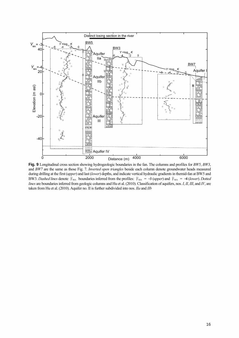
A longitudinal cross section is generated by using the geologic columns and MAY profiles, as shown in Fig. 9. This cross section extends from the fan-apex 2-km upstream of BW5 to the fan-toe at BW7. The two dotted lines are the boundaries determined from only the stratigraphic information. The lower dotted line is related to the boundary between the Pleistocene nos. III and IV aquifers, which is distributed throughout the cross section at an elevation of around -50 meters above sea level (m asl) according to Hu et al. (2010). The upper dotted line represents the boundary between the Holocene nos. I and II aquifers, which is determined to be ~10 m asl at BW7. These dotted lines are relatively distinguishable because of the sudden stratigraphic change between the gravel fan deposits and the fine fluvial deposits. However, other boundaries of the gravel deposits such as between the Holocene no. II and Pleistocene no. III aquifers are hard to specify among the monotonic stratigraphic columns.

Two MAY boundaries are also traceable among the profiles: a lower broken line with MAY = -4 and an upper broken line with MAY = -3. The lower boundary is below a depth of ~30 m from the ground surface, and is at the same elevation as the hydrogeologic boundary between the Holocene no. II and Pleistocene no. III aquifers (Hu et al. 2010). This correspondence indicates that the Pleistocene no. III aquifer has only weak K depth dependence, and the permeability in the aquifer is assumed to be stationary at around the expectation of K = 10-4 m/s. In contrast, the upper boundary of MAY divides the Holocene no. II aquifer into two further aquifers: nos. IIa (upper) and IIb (lower). The Holocene no. IIa aquifer is

8

~10 m thick near the surface, and MAY > -3 here (i.e., K = 1 × 10-3 m/s). Such high values of K are similar to those found in previous pumping test results: pumping tests were conducted in shallow wells near BW5 and BW3, and obtained an average hydraulic conductivity of K ≈ 2 × 10-3 m/s (Hokkaido Regional Development Bureau 2008). The Holocene no. IIa aquifer is directly connected to the river bed, and the surface water is actively infiltrated through the aquifer due to its high permeability and vertical hydraulic gradients. Thus, the Holocene no. IIa aquifer along the river is of importance as an infiltrative aquifer. However, if the aquifer is at a distance of several hundred meters from the river, it is almost unsaturated since the groundwater surface slopes downward.

In the Holocene no. IIb aquifer, the permeability takes a wide ranges of values, from K = 1 × 10-5 to 1 × 10-2 m/s. This range is affected by the sedimentary texture at each depth. Conversely, the average permeability decreases with depth according to the exponential equation (Eq. (11)). As a result, the groundwater flows horizontally and vertically through the water passages, which are formed and affected by the geological heterogeneity and depth-dependent effects. Three-dimensional groundwater flows also influence solute transport. For example, the temperature profiles at BW5 and BW3 suggest the existence of large envelopes and a deepening of the isothermal layer. Typical temperature distributions are explained by the presence of strong heterogeneity, as well the depth dependence of the permeability, through a simulation that couples groundwater flow and heat transport (Sakata and Ikeda 2012b). Conclusions

The depth dependence of the hydraulic conductivity K in the Toyohira River alluvial fan was determined, and the trend was represented by an empirical exponential equation. The proposed method consisted of the following steps. (1) Relatively undisturbed and sequential gravel cores were sampled by using improved tube samplers. (2) The packing in gravel cores was categorized qualitatively into four levels, and then the length fraction of each packing level was measured per unit depth. After these measurements, the effective grain size (in the current case this was d20) was obtained by sieving. (3) The relation between the slug tests and core properties was established through optimization. (4) Core properties profiles were transformed into those of the estimated hydraulic conductivity K by using the established relation. (5) A moving average method was applied to eliminate errors. In the present case, an average interval of 5 m was used. (6) A linear regression analysis revealed the depth dependence of K in the mid-fan, and the decay exponent was estimated.

The depth dependence of K was shown at the sampling points BW5 and BW3, and the decreasing trend had a decay exponent of A = 0.11 m-1, which is 10- to 1000-fold that for consolidated rock in the literature. Conversely, at BW7 in the fan-toe, a vertical trend was not observed. A longitudinal cross section was further generated by using the moving average profiles. Moving average boundaries of MAY = -4 and MAY = -3 classified the gravel aquifer without migration succession. As a result, the hydrogeologic structures were understood as a high infiltrative aquifer (Holocene no. IIa), a depth-dependent and heterogeneous aquifer (Holocene no. IIb) and a stationary permeable aquifer (Pleistocene no. III).

Several problems remained unsolved in this study. The relation between the slug tests and core properties has not been sufficiently verified either theoretically or experimentally. Moreover, the obtained relation was applied only in the fan, and individual relations must be established at each site. The sampling error of the sampler has not been assessed experimentally (e.g., by comparison with bulk sampling). The scale at which permeability was observed in this study (i.e., unit depth) is not necessarily appropriate at other sites, and the employed scale must be discussed in terms of each hydrogeologic unit (Anderson 1989). Furthermore, the proposed method provided only vertical information at the sampling points. Thus, for three-dimensional groundwater modeling, horizontal information must be acquired by other methods such as outcrop analyses, geophysics surveys, geophysical logs, and deterministic depositional models. In spite of these issues, the proposed field method is expected to be useful for gaining greater quantitative insight into the depth dependence of the permeability in unconsolidated gravel deposits. Acknowledgments

The authors acknowledge the Hokkaido Regional Development Bureau, the administrator of the Toyohira River, for providing core samples, slug test data and technical reports. Special thanks are given to Prof. Satoshi Okamura of the Hokkaido University of Education and Dr. Tsumoru Sagayama of the Geological Survey of Hokkaido, who performed volcanic ash analysis and diatom analysis on the BW7 core, respectively. Helpful comments about the geology in the fan from Mr. Daisuke Nagaoka of Raax Co., Ltd. and Dr. Kenji Kizaki were also received with gratitude. Comments from the reviewer John Ong, the Associate Editor Bayani M Cardenas, and the Editor Maria-Theresia Schafmeister have helped us make substantial improvements in the manuscript.

9

References Anderson MP (1989) Hydrogeologic facies models to delineate large-scale spatial trends in glacial and glaciofluvial sediments. GSA Bull 101:501–511. doi:10.1130/0016-7606 ASCE (American Society of Civil Engineers) (2008) Standard guideline for fitting saturated hydraulic conductivity using probability density functions (ASCE EWRI 50–08), ASCE, Reston, VA Cardenas MB, Jiang XW (2010) Groundwater flow, transport, and residence times through topography-driven basins with exponentially decreasing permeability and porosity. Water Resour Res 46, W11538. doi :10.1029/2010WR009370 Chen X (2011) Depth-dependent hydraulic conductivity distribution patterns of a streambed. Hydrol Proc 25:278–287. doi:10.1002/hyp.7844 Cheong JY, Hamm SY, Kim HS, Ko EJ, Yang K, Lee JH (2008) Estimating hydraulic conductivity using grain-size analyses, aquifer tests, and numerical modeling in a riverside alluvial system in South Korea. Hydrogeol J 16:1129–1143. doi:10.1007/s10040-008-0303-4 Daimaru H (1989) Holocene evolution of the Toyohira River alluvial fan and distal floodplain, Hokkaido, Japan. Geophys Rev Japan 62A–8:589–603 dell’Arciprete D, Bersezio R, Felletti F, Giudici M, Comunian A, Renard P (2012) Comparison of three geostatistical methods for hydrofacies simulation: a test on alluvial sediments. Hydrogeol J 20:299–311. doi:10.1007/s10040-011-0808-0 de Marsily G (1986) Quantitative hydrogeology. Academic press, London Domenico PA, Shwartz FW (1998) Physical and chemical hydrogeology, 2nd edn. Wiley, New York Einsele G (2000) Sedimentary Basins, 2nd edn. Springer, Heidelberg Falivene O, Cabrera L, SáezLarge A (2007) Large to intermediate-scale aquifer heterogeneity in fine-grain dominated alluvial fans (Cenozoic as Pontes Basin, northwestern Spain): insight based on three-dimensional geostatistical reconstruction. Hydrogeol J 15:861–876. doi 10.1007/s10040-007-0187-8 Ferreira JT, Ritzi Jr. RW, Dominic DF, (2010) Measuring the permeability of open-framework gravel. Ground Water 48:593–597. doi: 10.1111/j.1745-6584.2010.00675.x Fetter CW (2001) Applied hydrogeology, 4th edn. Prentice-Hall, Upper Saddle River Freeze RA, Cherry JA (1979) Groundwater. Prentice-Hall, Englewood Cliffs, NJ Heinz J, Kleineidam S, Teutsch G, Aigner T (2003) Heterogeneity patterns of Quaternary glaciofluvial gravel bodies (SW-Germany): application to hydrogeology. Sediment Geol 158:1–23 Hess KM, Wolf SH, Celia MA (1992) Large-scale natural gradient tracer test in sand and gravel, Cape Cod, Massachusetts: 3. Hydraulic conductivity variability and calculated macrodispersivities. Water Resour Res 28:2011–2027. doi:10.1029/92WR00668 Hokkaido Regional Development Bureau (2006) Toyohiragawa hoka kasyou zairyou chousa gyoumu houkokusyo [Investigation report on riverbed material in the Toyohira River]. Hokkaido Regional Development Bureau, Sapporo, Japan Hokkaido Regional Development Bureau (2008) Toyohiragawa sougou mizu kanri kentou gyoumu houkokusyo [Investigation report on comprehensive water management of the Toyohira River]. Hokkaido Regional Development Bureau, Sapporo, Japan Hu SG, Miyajima S, Nagaoka D, Koizumi K, Mukai K (2010) Study on the relation between groundwater and surface water in Toyohira-gawa alluvial fan, Hokkaido, Japan. In: Taniguchi M, Holman IP (eds.) Groundwater response to changing climate. CRC Press, London. doi: 10.1201/b10530-13 Hvorslev MJ (1951) Time lag and soil permeability in ground water observations. USACE: WES, Bull. 36:1–50 Ingebritsen SE, Sanford WE, Neuzil CE (2006) Groundwater in geologic processes, 2nd edn. Cambridge university press, Cambridge JGS (Japan Geotechnical Society) (2004) Method for determination of hydraulic properties of aquifer in single borehole. In: Japanese standards for geotechnical and geoenvironmental investigation methods, JGS, Tokyo Jiang XW, Wan L, Wang XS, Ge S, Liu J (2009) Effect of exponential decay in hydraulic conductivity with depth on regional groundwater flow. Geophys Res Lett 36, L24402. doi: 10.1029/2009GL041251 Jiang XW, Wang XS, Wan L (2010) Semi-empirical equations for the systematic decrease in permeability with depth in porous and fractured media. Hydrogeol J 18:839–850. doi: 10.1007/s10040-010-0575-3 Jussel P, Stauffer F, Dracos T (1994) Transport modeling in heterogeneous aquifers: 1. statistical description and numerical generation of gravel deposits. Water Resour Res 30:1803–1817 Kamann PJ, Ritzi RW, Dominic DF, Conrad CM. (2007) Porosity and permeability in sediment mixtures. Ground Water 45: 429–438. doi: 10.1111/j.1745-6584.2007.00313.x Koltermann CE, Gorelick SM (1995) Fractional packing model for hydraulic conductivity derived sediment mixtures. Water Resour Res 31:3283–3297 Koltermann CE, Gorelick SM (1996) Heterogeneity in sedimentary deposits: a review of structure-Imitating, process-imitating, and descriptive approaches. Water Resour Res 32:2617–2658. doi: 10.1029/96WR00025 Kresic N (2007) Hydrogeology and groundwater modeling, 2nd edn. CRC Press, Boca Raton, FL Lu C, Chen X, Chen C, Ou G, Shu L (2012) Horizontal hydraulic conductivity of shallow stream bed sediments and comparison with the grain-size analysis results. Hydrol Proc 26:454–466. doi: 10.1002/hyp.8143 Lunt IA, Bridge JS (2007) Formation and preservation of open-framework gravel strata in unidirectional flows. Sedimentol

10

54:71–87. doi: 10.1111/j.1365-3091.2006.00829.x Lunt IA, Bridge JS, Tye RA (2004) A quantitative, three-dimensional depositional model of gravelly braided rivers. Sedimentol 41:377–414. doi: 10.1111/j.1365-3091.2004.00627.x Luo W, Grudzinski B, Pederson D (2011) Estimating hydraulic conductivity for the Martian subsurface based on drainage patterns—a case study in the Mare Tyrrhenum Quadrangle. Geomorphol 125:414–420. doi:10.1016/j.geomorph.2010.10.018 Major JJ (1997) Depositional processes in large-scale debris-flow experiments. J Geol, 105:345–366. doi:10.1086/515930 Major JJ (2000) Gravity-driven consolidation of granular slurries: implications for debris-flow deposition and deposit characteristics. J Sediment Res 70:64–83. doi: 10.1306/2DC408FF-0E47-11D7-8643000102C1865D Manning CE, Ingebritsen SE (1999) Permeability of the continental crust: implications of geothermal data and metamorphic systems. Rev Geophys 37:127–150. doi:10.1029/1998RG900002 Marion A, Packman AI, Zaramella M, Bottacin-Busolin A (2008) Hyporheic flows in stratified beds. Water Resour Res 44, W09433. doi: 10.1029/2007WR006079 Matsumoto N, Yamaguchi Y (1991) Interaction between stress and permeability in sand and gravel deposit. J Geotech Eng 430:59–67 McElwee CD, Butler Jr. JJ, Healey JM (1991) A New sampling system for obtaining relatively undisturbed samples of unconsolidated coarse sand and gravel. Ground Water Monit Remediat 11: 182–191, doi: 10.1111/j.1745-6592.1991.tb00390.x Miall AD (1992) Alluvial deposits. In: Walker RG, James NP (eds.) Facies models response to sea level change. Geological Association of Canada, Toronto Morin RH (2006) Negative correlation between porosity and hydraulic conductivity in sand-and-gravel aquifers at Cape Cod, Massachusetts, USA. J Hydrol 316:43–52. doi:10.1016/j.jhydrol.2005.04.013 Oka T (2005) Analyzing the subsurface geologic structure of the central part of Sapporo City and its northwest suburb by drilling data of fluid resources, with notes on geological explanation for six profiles of seimic prospecting performed by the municipal authorities of Sapporo City and so on. Rep Geol Surv Hokkaido 76:1–54 Neton MJ, Dorsch J, Olson CD, Young SC (1994) Architecture and directional scales of heterogeneity in alluvial-fan aquifers. J Sediment Res 64B:245–257. Rubin Y (2003) Applied stochastic hydrogeology. Oxford university press, New York Saar MO, Manga M (2004) Depth dependence of permeability in the Oregon Cascades inferred from hydrogeologic, thermal, seismic, and magmatic modeling constraints. J Geophys Res 109(B04204). doi:10.1029/2003JB002855 Sakata Y, Ikeda R (2012a) Quantification of longitudinal river discharge and leakage in an alluvial Fan by synoptic survey using handheld ADV. J Japan Soc Hydrol Water Res 25:89–102 Sakata Y, Ikeda R (2012b) Effectiveness of a high resolution model on groundwater simulation in an alluvial fan. Geophys Bull Hokkaido University 75:73–89 Sakata Y, Ito K, Isozaki S, Ikeda R (2011) A distribution model of permeability derived from undisturbed gravelly samples in alluvial fan. Japanese Geotech J 6:109–119 Shepherd RG (1989) Correlations of permeability and grain size. Ground Water 27:633–638. doi: 10.1111/j.1745-6584.1989.tb00476.x Singhal BBS, Gupta RP (1999) Applied hydrogeology of fractured rocks. Kluwer Academic Publishers, Dordrecht Snow DT (1969) Anisotropic permeability of fractured media. Water Resour Res 5:1273–1289. doi:10.1029/WR005i006p01273 Song J, Chen X, Cheng C, Wang D, Lackey S, Xu Z (2009) Feasibility of grain-size analysis methods for determination of vertical hydraulic conductivity of streambeds. J Hydrol 375:428–437. doi:10.1016/j.jhydrol.2009.06.043 Tanaka Y, Kudo K, Yosida Y, Nisi K, Aida M, Suzuki H (1990) On the applicability of various sampling methods to the gravelly ground. Cent Res Inst Electr Power Industry, Abiko Res Lab Rep No U90046 Todd DK, Mays LW (2005) Groundwater Hydrology, 3rd edn. Wiley, New York Vienken T, Dietrich P (2011) Field evaluation of methods for determining hydraulic conductivity from grain size data. J Hydrol 400:58–71. doi:10.1016/j.jhydrol.2011.01.022 Vukovic M, Soro A (1992) Determination of hydraulic conductivity of porous media from grain-size composition. Water Resources Publications, Littleton Wackernagel H (2010) Multivariate geostatistics: an introduction with applications, 3rd edn. Springer, Berlin Wang XS, Jiang XW, Wan L, Song G, Xia Q (2009) Evaluation of depth-dependent porosity and bulk modulus of a shear using permeability–depth trends. Int J Rock Mech Min Sci 46:1175–1181. doi:10.1016/j.ijrmms.2009.02.002 Yamaguchi H, Osanai H, Sato O, Futamase K, Obara T, Hayakawa F, Yokoyama E (1965). Explanatory text of hydrogeological maps of Hokkaido no. 8, Sapporo, special part “the grounds and groundwater of Sapporo environments.” Geological survey of Hokkaido, Sapporo, Japan Zappa G, Bersezio R, Felletti F, Giudici M (2006) Modeling heterogeneity of gravel-sand, braided stream, alluvial aquifers at the facies scale. J Hydrol 325:134-153. doi:10.1016/j.jhydrol.2005.10.016 Zlotnik VA, Cardenas MB, Toundykov D (2011) Effects of multiscale anisotropy on basin and hyporheic groundwater Flow. Ground Water 49:576–583. doi: 10.1111/j.1745-6584.2010.00775.x

11

Fig. 1 Location maps and geologic features of the study area: the Toyohira River alluvial fan. Solid circles represent undisturbed sampling points, BW1–7; dashed lines denote groundwater-level contours with elevation values (in meters above sea level) measured in June 2010; and KP values denote the distance (in km) along the river channel upward from the confluence of the Ishikari River

Fig. 2 Schematic of improved double core-tube sampler used in this study (ACE Shisui, Co., Ltd., Japan)

12

Fig. 3 Classification of gravel core according to matrix packing level. Packing levels I and II at unit depth are grouped as the high packing part; packing levels III and IV are grouped as the low packing part

Fig. 4 Box and whisker plots showing the vertical statistics of length fractions of low packing parts a. L3 and b. L4. Summaries are given at 10-m intervals of depth Z. Solid squares above each box denote measurements at BW1-7, the left- and right-hand side bars of the boxes respectively denote the 25th and 75th percentiles, the bars within the boxes denote the medians, the bars at the left and right ends of the whiskers respectively denote the minimum and maximum values and open squares in the boxes denote the averages. Some of the median bars are not visible because their values are equal to zero

13

Table 1 Analysis data and results for optimal determination of a relationship between slug tests and gravel cores, in the Toyohira-gawa alluvial fan.

a Effective grain-size diameter by sieving (mm) b Length fraction of each packing level (m/m) c Common logarithm of K (m/s) measured by slug test results (modified to a constant temperature

of 25 °C) d Common logarithm of K (m/s) estimated by Eq. (8) e Residual log-conductivity between Y and Y

Properties of gravel cores Log-conductivity Sample number

Point ID

Sampling and test depth (m) d20

a L1+L2 b L3

b L4 b Y c Y d ReY e

1 BW1 9 - 10 0.85 0.91 0.00 0.09 -2.62 -2.86 0.24

2 BW2 5 - 6 12 0.29 0.53 0.18 -2.05 -1.86 -0.19

3 8 - 9 1.6 0.80 0.18 0.02 -3.16 -3.86 0.70

4 BW3 3 - 4 0.83 0.50 0.40 0.10 -2.55 -2.53 -0.02

5 9 - 10 3.7 0.43 0.42 0.15 -2.76 -2.12 -0.64

6 19 - 20 2.4 1.00 0.00 0.00 -4.09 -4.12 0.03

7 29 - 30 8.6 0.66 0.25 0.09 -2.50 -2.66 0.16

8 31 - 32 0.70 0.91 0.09 0.00 -5.15 -4.73 -0.42

9 39 - 40 4.2 0.81 0.19 0.00 -3.58 -3.54 -0.04

10 49 - 50 1.0 1.00 0.00 0.00 -5.35 -4.86 -0.49

11 59 - 60 3.0 1.00 0.00 0.00 -4.14 -3.94 -0.20

12 BW4 5 - 6 1.0 0.82 0.09 0.09 -3.22 -2.86 -0.36

13 8 - 9 0.63 0.60 0.40 0.00 -3.51 -2.97 -0.54

14 BW5 3 - 4 2.2 0.71 0.29 0.00 -3.00 -3.35 0.35

15 9 - 10 2.0 1.00 0.00 0.00 -4.80 -4.29 -0.51

16 19 - 20 3.3 0.85 0.15 0.00 -3.65 -3.77 0.12

17 29 - 30 1.5 0.93 0.00 0.07 -3.67 -3.18 -0.49

18 39 - 40 0.71 1.00 0.00 0.00 -4.64 -5.15 0.51

19 59 - 60 2.1 1.00 0.00 0.00 -4.48 -4.24 -0.24

20 69 - 70 0.86 0.90 0.10 0.00 -5.03 -4.58 -0.45

21 89 - 90 1.43 0.92 0.08 0.00 -4.66 -4.47 -0.19

22 BW6 6 - 7 2.1 1.00 0.00 0.00 -4.56 -4.26 -0.30

23 9 - 10 5.2 0.93 0.04 0.03 -3.03 -3.46 0.43

24 18 - 19 4.4 0.84 0.11 0.05 -3.63 -3.35 -0.28

25 BW7 10 - 11 2.8 1.00 0.00 0.00 -3.79 -4.01 0.22

26 14 - 15 1.3 1.00 0.00 0.00 -3.76 -4.65 0.89

27 18 - 19 1.0 0.77 0.13 0.10 -2.28 -2.72 0.44

28 23 - 24 0.81 0.94 0.00 0.06 -2.99 -3.38 0.39

29 29 - 30 0.55 0.96 0.00 0.04 -3.55 -3.91 0.36

30 33 - 34 2.2 0.88 0.03 0.09 -2.82 -2.85 0.03

31 37 - 38 1.1 0.82 0.18 0.00 -3.43 -3.96 0.53

32 43 - 44 1.1 1.00 0.00 0.00 -4.85 -4.81 -0.04

Mean 0.00 Variance 0.16

14

Fig. 5 Comparison in double logarithmic scale between hydraulic conductivities measured by slug test, K (m/s), and estimated by Eq. (8) ( K (m/s)). Here, R2 = 0.80

Fig. 6 Curves relating K calculated by Eq. (8) and effective grainsize diameter –φ d20 = log2 d20 (mm) for several length fractions of low packing part L3 or L4 (m/m)

15

Fig. 7 Core property and hydraulic conductivity results at a. BW5, b. BW3 and c. BW7. Each set of results contains, from left to right: the geologic column; effective grain-size diameters, –φ = log2 d20 (mm); length fractions of low packing part, L3 (gray bars) and L4 (dark gray bars) (m/m); and common logarithms of the hydraulic conductivity (m/s). In the log-conductivity profiles, solid squares denote Y values measured by slug tests, open squares denote Y values estimated by Eq. (8) and solid lines denote moving average MAY values over 5-m intervals. All data are obtained at unit depth. Gaps represent depths at which data were rejected or not obtained

Fig. 8 Scatter plot of MAY values at BW5, BW3, and BW7 with associated regression lines. Solid squares denote MAY values at BW5, open circles denote values at BW3, and solid triangles denote values at BW7. Averages are plotted at mid-depths of 5-m intervals. A regression analysis between MAY and depth is conducted in each well using data above a depth of 40 m

16

Fig. 9 Longitudinal cross section showing hydrogeologic boundaries in the fan. The columns and profiles for BW5, BW3, and BW7 are the same as those Fig. 7. Inverted open triangles beside each column denote groundwater heads measured during drilling at the first (upper) and last (lower) depths, and indicate vertical hydraulic gradients in themid-fan at BW5 and BW3. Dashed lines denote MAY boundaries inferred from the profiles: MAY = －3 (upper) and MAY = －4 (lower). Dotted lines are boundaries inferred from geologic columns and Hu et al. (2010). Classification of aquifers, nos. I, II, III, and IV, are taken from Hu et al. (2010). Aquifer no. II is further subdivided into nos. IIa and IIb