The Dark Side of Analyst Coverage: The Case of Innovation

Jie (Jack) He Terry College of Business

University of Georgia jiehe@uga.edu (706) 542-9076

Xuan Tian Kelley School of Business

Indiana University tianx@indiana.edu

(812) 855-3420

This version: June, 2012

* We are grateful for helpful comments from Utpal Bhattacharya, Matthew Billett, Daniel Bradley, Alex Edmans, Stuart Gillan, Harrison Hong, David Hsu, Paul Irvine, Sreenivas Kamma, Robert Kieschnick, Josh Lerner, Jim Linck, Harold Mulherin, Jeff Netter, Bradley Paye, Tao Shu, Scott Smart, Krishnamurthy Subramanian, Scott Yonker, and Xiaoyun Yu, conference participants at the 2012 Kauffman-RCFP Entrepreneurial Finance and Innovation conference, and seminar participants at Indiana University and the University of Georgia. We thank Zhong Zhang for his competent research assistance. We remain responsible for any remaining errors or omissions.

The Dark Side of Analyst Coverage: The Case of Innovation

Abstract

We examine the effect of analyst coverage on firm innovation. Our baseline results show that firms covered by a larger number of analysts generate fewer patents and patents with lower impact. The evidence is consistent with the hypothesis that analysts exert too much pressure on managers to meet short-term goals, impeding firms’ investment in long-term innovative projects. To establish causality, we use a difference-in-differences approach that relies on the variation generated by multiple exogenous shocks to analyst coverage, as well as an instrumental variable approach. Our identification strategies suggest a causal effect of analyst coverage on firm innovation and the effect is stronger when firms are covered by fewer analysts. Further, we show that the negative effect of analyst coverage on firm innovation is much more pronounced when the firm is about to just miss its earnings target, but is mitigated when managers are protected by various “pressure shields” such as larger equity holdings by institutional investors who actively gather information about firm fundamentals and a higher level of managerial entrenchment. Finally, we discuss two possible mechanisms through which analysts impede innovation: the severe consequences of missing earning targets and the difficulty of implementing accrual-based earnings management. Our paper offers novel evidence on a previously under-explored adverse consequence of analyst coverage — its hindrance to firm innovation.

Key words: analyst coverage, innovation, patents, citations, managerial myopia JEL number: G24, O31, G34

1

1. INTRODUCTION

How does stock market oversight affect firm innovation? Specifically, do financial

analysts, an active market player and gatekeeper, encourage or impede firm innovation?

Although there has been a growing literature linking various market and firm characteristics to

innovation, little is known about the effects of financial analysts. Understanding the role of

financial analysts in motivating firm innovation is an important research question, because

innovation is one of the most crucial drivers of economic growth (Solow, 1957) and analyst

behavior in the U.S. is heavily regulated and can be altered by securities laws and regulations.1

The objective of this paper is to provide the first empirical study that examines how financial

analysts affect firm innovation, using a rich set of identification strategies.

Innovation is vital for the long-run competitive advantage of firms. However, motivating

innovation remains a challenge for most firms. Unlike routine tasks, such as mass production and

marketing, innovation involves a long process that is full of uncertainty and with a high

probability of failure (Holmstrom, 1989). Firms investing more heavily in innovative projects

might be forced to make only partial disclosure and subject to a larger degree of information

asymmetry (Bhattacharya and Ritter, 1983), are more likely to be undervalued by equity holders,

and have a greater exposure to hostile takeovers (Stein, 1988). To protect firms against such

expropriation, managers tend to invest less in innovation (in many cases sub-optimally) and put

more effort in routine tasks that offer quicker and more certain returns, leading up to a typical

managerial myopia problem. A potential solution to the distortion of investments in innovation

due to information asymmetry is financial analysts. Financial analysts collect information from

various sources, evaluate the current performance of firms that they follow, make forecasts about

their future prospects, and make buy/hold/sell recommendations to current and potential

investors. Existing literature suggests that analysts help to reduce information asymmetry along a

variety of dimensions (see a detailed discussion of this literature in Section 2). If analysts

accurately convey the information of a firm’s innovative activities to other financial market

participants (especially its investors) and help them understand the real value of these long-term

investments, then the management of the firm would not refrain from engaging in value-

enhancing innovation activities. Therefore, our first hypothesis, the “information hypothesis”,

1 Recent regulatory changes include the 2000 Regulation Fair Disclosure (Reg FD), the 2002 National Association of Securities Dealers (NASD) Rule 2711, and the 2003 Global Research Analyst Settlement, among others.

2

argues that financial analysts, by reducing information asymmetry of innovative firms, mitigate

managerial myopia and encourage firm innovation.2

An alternative hypothesis makes an opposite empirical prediction. Financial analysts are

often accused of creating excessive pressure on managers and exacerbating managerial myopia.

Manso (2011) theoretically shows that tolerance for failure is necessary for effectively

motivating and nurturing innovation.3 However, the least thing financial analysts can offer to

innovative firms is to tolerate short-term failures, as their job is to forecast near-term earnings

and make corresponding stock recommendations. Whenever they expect the firms to experience

a drop in near-term earnings, they would revise their forecasts downward and make unfavorable

recommendations, leading to negative market reactions and potential disciplinary actions against

the managers (see, e.g., Brennan, Jegadeesh, and Swaminathan, 1993; Hong, Lim, and Stein,

2000). More importantly, just as Jensen and Fuller (2002) argued, firm managers all too often

conform to excessively aggressive analysts’ earnings forecasts and accept external expectations

as targets to achieve. In a survey of 401 U.S. Chief Financial Officers (CFOs), Graham, Harvey,

and Rajgopal (2005) show that the majority of CFOs in the survey declared that they are willing

to sacrifice long-term firm value to meet the desired short-term earnings targets due to their own

wealth, career, and external reputation concerns.4 Innovation ranks high on the list that managers

consider sacrificing due to its nature of being a type of high-risk, long-term, and unpredictable

investment that may not generate immediate financial returns. Taken together, the alternative

hypothesis we propose, the “pressure hypothesis”, argues that financial analysts, by imposing

short-term pressures on managers, exacerbate managerial myopia and impede firm innovation.

We test the above two competing hypotheses by examining whether financial analysts

mitigate or exacerbate managerial myopia. As pointed out by Stein (2003), “Managerial myopia

is difficult to test because it results in underinvestment in activities that are difficult to observe.”

2 Note that moral hazard models such as Grossman and Hart (1988) and Harris and Raviv (1988) may generate the same prediction as the information hypothesis. These models suggest that managers who are not properly monitored will shirk or tend to invest sub-optimally in routine tasks with quicker and more certain returns to enjoy private benefits. If managers derive private benefits from shirking on long-term innovation projects (as suggested by the above theories) and financial analysts serve as an external governance mechanism (Yu, 2008), the above moral hazard argument also implies that financial analysts encourage corporate innovation. 3 Recent empirical research providing supporting evidence for the implications of the failure tolerance theory includes Ederer and Manso (2011), who conduct a controlled laboratory experiment, and Azoulay, Graff Zivin, and Manso (2011), who exploit key differences among funding streams within the academic life science. 4 The adverse consequences for managers to miss the consensus earnings forecasts include significant declines in the firms’ stock prices (Bartov, Givoly, and Hayn, 2002), reduced CEO bonuses (Matsunaga and Park, 2001), and an increased probability of management turnover (Mergenthaler, Rajgopal, and Strinivasan, 2011).

3

We make use of an observable investment output (i.e., the number of patents granted to a firm

and the number of future citations received by each patent) to assess the success of long-term

investment and investment in intangible assets that have traditionally been difficult to observe.

One key advantage of using patenting rather than R&D expenditures to capture

innovation activities is that patenting is an innovation output variable, which encompasses the

successful usage of all (both observable and unobservable) innovation inputs. In contrast, R&D

expenditures only capture one particular observable input of innovation and fail to account for

many other (equally or even more important) observable or unobservable inputs such as the

allocation of talent, effort, and attention to innovative projects and internal incentive schemes

(especially non-monetary ones such as public acknowledgements).5 In addition, information on

R&D expenditures reported in the Compustat database is quite unreliable.6 Our strategy of using

patenting to capture firms’ innovativeness significantly reduces the measurement error concern

and has now become standard in the innovation literature (e.g., Aghion et al., 2005; Chemmanur

et al., 2011; Nanda and Rhodes-Kropf, 2011a).

Our baseline tests show a negative relation between analyst coverage (measured by the

number of analysts following the firm) and innovation output. An increase in analyst coverage

from the 25th to the 75th percentile of its distribution is associated with a 10.2% decrease in the

number of patents generated in the next year and a 22.8% decrease in the number of future

citations received by the patent generated in the next year. The results are robust to alternative

measures of analyst coverage and innovation output as well as alternative empirical and

econometric specifications.

While the baseline results are consistent with the pressure hypothesis, an important

concern is that analyst coverage is likely to be endogenous. Unobservable firm heterogeneity

correlated with both analyst coverage and innovation could bias the results towards our baseline

findings (i.e., the omitted variables concern), and firms with low innovation potential may attract

5 Recent innovation literature also makes a similar argument, pointing out that R&D represents only one particular observable quantitative input (see, e.g., Aghion, Van Reenen, and Zingales, 2012) and is sensitive to accounting norms such as whether it should be capitalized or expensed (see, e.g., Acharya and Subramanian, 2009). 6 More than 50% of firms do not report R&D expenditures in their financial statements in the Compustat database. However, the fact that a firm does not report its R&D expenditures does not necessarily mean that the firm is not engaging in innovation activities. It may do so out of strategic concerns. Replacing missing values of R&D expenditures with zeros, a common practice in the existing literature, introduces additional noise that may bias the estimated effect of analyst coverage on innovation measured by R&D expenditures.

4

more analyst coverage (i.e., the reverse causality concern). To establish causality, we use two

different identification strategies and perform a rich set of identification tests.

Our first identification strategy is to rely on two plausible quasi-natural experiments,

brokerage closures (Kelly and Ljungqvist, 2011, 2012) and brokerage mergers (Hong and

Kacperczyk, 2010), that directly affect firms’ analyst coverage but are exogenous to their

innovation productivity. Using a difference-in-differences (DiD) approach, we show that an

exogenous decrease in analyst coverage results in a smaller decrease in the level of innovation

output for the treatment group (i.e., firms that lose one analyst due to brokerage closures and

mergers) compared to that for the control group (i.e., similar firms whose analyst coverage do

not change) in subsequent years. Further, the negative effect of analyst coverage on innovation is

stronger for firms covered by fewer analysts. A key advantage of this identification strategy is

that there are multiple shocks in this setting that affect different firms at exogenously different

times, which avoids a common identification difficulty faced by studies with a single shock,

namely, the existence of potential omitted variables coinciding with the shock that directly affect

firm innovation.

Our second identification strategy is to construct an instrumental variable, expected

coverage, first introduced in Yu (2008), and to use the two-stage least-squares (2SLS) analysis.

The 2SLS results confirm the negative effect of analyst coverage on innovation and, more

importantly, reveal the direction of potential bias if endogeneity in analyst coverage is not

appropriately controlled for. Overall, our identification tests suggest that analysts have a negative

causal effect on firm innovation.

We explore our baseline results further by examining how analysts affect firm innovation

differently in the cross section. We first use the cross-sectional variation in the degree to which a

firm is about to miss its earnings target. If managers indeed conform to the short-term pressure

imposed by analysts, their incentives to reduce investments in innovative projects should be

stronger when they are expected to just miss the earnings target. Consistent with this conjecture,

we find that the negative effect of analyst coverage on firm innovation is much more pronounced

when the firm is about to just miss its earnings target. Next, we explore the cross-sectional

variation in some “pressure shields” that insulate managers, to some extent, from the short-term

pressure imposed by financial analysts. Since analysts do not make direct decisions on

managerial turnover or compensation, the magnitude of their pressure on firm management

5

crucially depends on the bargaining power of managers against shareholders and the latter’s

emphasis on firms’ short-term performance. If analysts indeed exert pressure on managers, then

we expect the negative effect of analyst coverage on firm innovation to be less pronounced when

managers have greater bargaining power over shareholders or when shareholders care less about

firms’ short-term performance, i.e., when the managers are “insulated” from the pressure to meet

short-term goals. The two “pressure shields” we examine are equity holdings by dedicated

institutional investors who actively gather information about firm fundamentals and managerial

entrenchment. We show that the negative effect of financial analysts on innovation is mitigated

when a larger share of equity is held by dedicated institutional investors and when managers are

more entrenched.7

Finally, we discuss two possible mechanisms through which analysts impede innovation.

The first mechanism is the severe consequences of missing earnings targets when the firm is

followed by a large number of analysts. We show that the cumulative abnormal returns (CARs)

upon a negative earnings surprise (i.e., missing analysts’ consensus forecast targets) are larger in

magnitude (i.e., more negative) when the firm is covered by more analysts. The second

mechanism is the increased difficulty of implementing accrual-based earnings management for

firms with a high level of analyst coverage.

Overall, our evidence is consistent with the pressure hypothesis that analysts exert

pressure on managers to meet near-term earnings targets. In response to the pressure imposed by

analysts, managers boost current earnings by sacrificing long-term innovative projects that are

highly risky and slow in generating revenues.

The rest of the paper is organized as follows. Section 2 discusses the related literature.

Section 3 discusses sample selection and reports summary statistics. Section 4 presents the

baseline results and robustness checks. Section 5 addresses identification issues. Section 6

reports cross-sectional analysis. Section 7 discusses possible mechanisms. Section 8 concludes.

2. RELATION TO THE EXISTING LITERATURE

Our paper contributes to three strands of literature. First, our paper is related to the

emerging literature on finance and firm innovation. Holmstrom (1989) theoretically shows that

7 In unreported analysis, we also consider two more “pressure shields” related to firms’ recent performance. Specifically, we find that the negative effect of analyst coverage on firm innovation is mitigated when firms’ recent stock market performance (e.g., average stock returns) and operating performance (e.g., return on assets) are better.

6

innovation activities may mix poorly with routine activities in an organization. Manso (2011)

suggests that managerial contracts that tolerate failure in the short run and reward for success in

the long run are best suited for motivating innovation. The model in Ferreira, Manso, and Silva

(2012) argues that it is optimal for firms to be private (literally having no analyst coverage) when

they want to innovate. Empirical evidence shows that various economic environment and firm

characteristics affect managerial incentives of investing in innovation. Specifically, a larger

institutional ownership (Aghion, Van Reenen, and Zingales, 2012), corporate venture capitalists

(Chemmanur et al., 2011), debtor-friendly bankruptcy laws (Acharya and Subramanian, 2009),

and lower stock liquidity (Fang, Tian, and Tice, 2011) help mitigate managerial myopia and

motivate managers to focus more on long-term innovation activities. Other studies have

examined the effect of product market competition, market conditions, leveraged buyouts,

investors’ failure tolerance, and corporate governance on firm innovation (e.g., Meulbroek et al.,

1990; Aghion et al., 2005; Nanda and Rhodes-Kropf, 2011a, 2011b; Lerner, Sorensen, and

Stromberg, 2011; Tian and Wang, 2011). However, existing studies have largely ignored the

roles played by financial analysts in motivating innovation. Our paper contributes to this line of

research by filling in this gap.

Our paper also builds on the empirical literature studying managerial myopia. This

literature has shown evidence consistent with managerial myopia in publicly traded firms.8 For

example, Asker, Farre-Mensa, and Ljungqvist (2011) find that listed firms exhibit myopia as,

compared to unlisted firms, they invest less and their investment levels are less sensitive to

changes in investment opportunities. Our paper complements their findings by providing a

possible reason, namely, the pressure imposed by financial analysts, for why listed firms are

more myopic than unlisted firms. Bushee (1998) shows that managers are more likely to cut

R&D expenses in response to an earnings decline when a very large proportion of institutional

ownership comes from short-term investors. Our paper instead focuses on the effect of financial

analysts on managerial myopia. We also use innovation output (patenting) rather than input

(R&D expenses) to capture firm managerial myopia.

Finally, our paper adds to the large literature debating on the real effects of financial

analysts. On the positive side, existing literature generally finds that financial analysts help

8 Stein (1989) theoretically shows that managerial myopia is present even in a rational capital market, and the degree of myopic behavior will be influenced by capital market incentives that determine the extent to which managers care about short-term prices relative to long-term values.

7

reduce information asymmetry, have superior predictive abilities, and serve as external monitors

to firm managers (e.g., Brennan and Subrahmanyam, 1995; Hong, Lim, and Stein, 2000; Das,

Guo, and Zhang, 2006; Yu, 2008; Ellul and Panayides, 2009), and therefore affect firms’

investment and financing decisions, stock prices, stock liquidity, and valuation (e.g., Bradley,

Jordan, and Ritter, 2003; Irvine, 2003; Chang, Dasgupta, and Hilary, 2006; Derrien and Kecskes,

2011; Kelly and Ljungqvist, 2011). On the negative side, Graham, Harvey, and Rajgopal (2005),

in a survey study, find that analysts put too much pressure on managers and induce myopic

behavior. There is a strategy literature that has provided some empirical support to the above

finding by using anecdotal evidence and small-sample analysis on a few industries. For example,

Benner (2010) shows that analysts tend to ignore firms’ strategies of incorporating new

technologies and pressure firms to make the “wrong” investments. Benner and Ranganathan

(2012) find that negative analyst recommendations are associated with reductions in firm capital

expenditure and R&D during times of technological change. However, it is hard to draw causal

inferences from the above two papers as they fail to address the identification issue. Moreover,

their sample sizes are small (fewer than 200 firms) and are limited in only a few industries. By

using a comprehensive large sample of U.S. public firms and a rich set of identification

strategies, our paper contributes to the above debate by examining the causal effect of analysts

on firm innovation — a special, long-term investment in intangible assets, and offers novel

evidence on a previously under-explored adverse effect of analysts.

Our paper is closely related to Barth, Kasznik, and McNichols (2001) who make an

important attempt to link analyst coverage to firm intangible assets. They show that analyst

coverage is positively associated with firm R&D expenditures. Our paper has two crucial

advantages over theirs. First, using both a difference-in-differences approach that relies on

multiple exogenous shocks to analyst coverage and an instrumental variable approach, our

identification strategies allow us to evaluate the causal effect of analyst coverage on firm

innovation (as opposed to a partial correlation documented by their study). Second, instead of

analyzing R&D expenditures, we focus on patenting activity. As we discussed in details before

(and in recent innovation literature), R&D data has various limitations to be used as a direct

measure of firms’ innovative activities. It only represents one particular observable quantitative

input (Aghion, Van Reenen, and Zingales, 2012), is sensitive to accounting norms such as

whether it should be capitalized or expensed (Acharya and Subramanian, 2009), and fails to fully

8

capture the quality of innovation. In contrast, patenting activity directly measures innovation

output and captures how effectively a firm has utilized all of its innovation input (both

observable and unobservable).

3. SAMPLE SELECTION AND SUMMARY STATISTICS 3.1 Sample Selection

The sample examined in this paper includes U.S. listed firms during the period of 1993-

2005. We collect firm-year patent and citation information from the latest version of the National

Bureau of Economic Research (NBER) Patent Citation database. Analyst coverage data are

obtained from the Institutional Brokers Estimate Systems (I/B/E/S) database. To calculate the

control variables, we collect financial statement items from Compustat, institutional holdings

data from Thomson's CDA/Spectrum database (form 13F), institutional investor classification

data from Brian Bushee’s website (http://acct3.wharton.upenn.edu/faculty/bushee), intraday

trades and quotes for constructing stock liquidity measures from the Trade and Quotes (TAQ)

database, stock price information from CRSP, and dual-class share structure as well as CEO

duality status from the RiskMetrics database. Finally, we obtain brokerage house merger

information from the Security Data Company (SDC) Mergers and Acquisitions database. The

sample selection procedure ends up with 33,521 firm-year observations.

3.2 Variable Measurement 3.2.1 Measuring Innovation

We extract innovation output data and construct our main innovation variables from the

latest version of the NBER Patent Citation database (see Hall, Jaffe, and Trajtenberg (2001) for

more details). This database contains updated patent and citation information from 1976 to 2006.

It provides annual information on patent assignee names, the number of patents, the number of

citations received by each patent, a patent’s application year as well as its grant year, etc. As the

patents appear in the database only after they are granted and it takes time for patents to receive

citations, following the existing innovation literature, we correct for the truncation problems in

the NBER Patent Citation database (see Appendix A for details).

It is worth noting that the patent database is unlikely to be affected by survivorship bias.

As long as a patent application is eventually granted, it is attributed to the applying firm at the

time of application even if the firm later gets acquired or goes bankrupt. Moreover, since patent

citations are attributed to a patent rather than the applying firm, the patent granted to a firm that

9

later gets acquired or goes bankrupt can still keep receiving citations long after the firm

disappears.

To gauge a firm’s innovation productivity, we construct two measures. The first measure

is a firm’s total number of patent applications filed in a given year that are eventually granted.

The reason for using a patent’s application year rather than its grant year is that previous studies

(such as Griliches, Pakes, and Hall, 1988) have shown that the former is superior in capturing the

actual time of innovation. However, despite its straightforward intuition and easy

implementation, the above measure is unable to distinguish groundbreaking innovations from

incremental technological discoveries. Hence, to assess a patent’s impact more precisely, we

construct the second measure of firm innovation productivity by counting the total number of

citations each patent receives in subsequent years. Given a firm’s size and its innovation inputs,

the number of patents captures its overall innovation productivity and the number of citations per

patent capture the significance and quality of its innovation output. To reflect the long-term

nature of innovation activities (especially its outcomes), in our empirical tests, we relate firm

characteristics in the current year to the above two measures of innovation productivity one, two,

three, and five years ahead.

We merge the NBER patent data with the analyst coverage sample. Following the

innovation literature, we set the patent and citation counts to zero for firms without available

patent or citation information from the NBER patent database. The distribution of patent grants

in our final sample is right skewed, with its median at zero. Due to the right skewness of patent

counts and citations per patent, we winsorize these variables at the 1st and 99th percentiles and

then use the natural logarithm of patent counts (LnPatent) and the natural logarithm of the

number of citations per patent (LnCitePat) as the main innovation measures in our analysis. To

avoid losing firm-year observations with zero patents or citations per patent, we add one to the

actual values when calculating the natural logarithm.

3.2.2 Measuring Analyst Coverage and Control Variables

We obtain analyst information from the I/B/E/S database. For each fiscal year of a firm,

we take the average of the 12 monthly numbers of earnings forecasts given by the summary file

and treat that as a raw measure of analyst coverage (Coverage). This measure relies on the fact

that most analysts following a firm issue at least one earnings forecast for that firm during the

year before its fiscal year ending date and that a majority of them issue at most one earnings

10

forecast in each month.9 We then take natural logarithm of (one plus) this raw measure and

construct our main measure of analyst coverage (LnCoverage).

Following the innovation literature, we control for a vector of firm and industry

characteristics that may affect a firm’s future innovation productivity. We compute all variables

for firm i over its fiscal year t. In the baseline regressions, our control variables include firm size

(the natural logarithm of book value assets), investments in intangible assets (R&D expenditures

over total assets), profitability (ROA), asset tangibility (net PPE scaled by total assets), leverage,

capital expenditure, growth opportunities (Tobin’s Q), financial constraints (the Kaplan and

Zingales (1997) five-variable KZ index), industry concentration (Herfindahl index based on

sales), institutional ownership, stock liquidity (the natural logarithm of relative effective

spreads), and firm age. To mitigate non-linear effects of product market competition on

innovation outputs (Aghion et al., 2005), we also include the squared Herfindahl index in our

baseline regressions. We provide detailed variable definitions in Appendix B.

3.3 Summary Statistics

To minimize the effect of outliers, we winsorize all variables at the 1st and 99th

percentiles. Table 1 provides summary statistics of the variables used in this study. On average, a

firm in our sample has 5.9 granted patents per year and each patent receives 4.7 citations, and is

followed by 6.8 analysts. Regarding other variables, an average firm has book value assets of

$3.47 billion, R&D-to-assets ratio of 5%, ROA of 9.2%, PPE-to-assets ratio of 28.7%, leverage

of 21.5%, capital expenditure ratio of 6.3%, Tobin’s Q of 2.1, and is 16.8 years old since its IPO

date.

4. EMPIRICAL RESULTS

4.1 Baseline Results To assess how analyst coverage affects innovation, we estimate the following model:

titititintinti YearFirmZLnCoverageLnCitePatLnPatent ,,,,, )( (1)

where i indexes firm, t indexes time, and n equals one, two, three, or five. The dependent

variables capture firm innovation outcomes: the natural logarithm of one plus the number of

9 However, to control for the possibility that a given analyst may give multiple forecasts within one month, we also calculate the total number of different analysts giving earnings forecasts for this firm during the 12-month period before its fiscal year ending date by using the historical detail file of I/B/E/S and find that the two measures of analyst coverage are highly correlated (with a Pearson correlation coefficient of 0.96). Thus, all our results remain unchanged if we use this alternative definition of analyst coverage.

11

patents filed (and eventually granted) (LnPatent) and the natural logarithm of one plus the

number of citations per patent (LnCitePat). Since the innovation process generally takes longer

than one year, we examine the effect of a firm’s analyst coverage on its patenting in subsequent

years. The analyst coverage measure, LnCoverage, is measured for firm i over its fiscal year t. Z

is a vector of firm and industry characteristics that may affect a firm’s innovation productivity as

we discussed in Section 3.2.2. Firm and Year capture firm fixed effects and fiscal year fixed

effects, respectively. We cluster standard errors at the firm level.

We include firm fixed effects in the baseline regressions because, as in most empirical

studies involving an endogeneity concern, it is possible that unobservable variables omitted from

our empirical model (equation (1)) affect both analyst coverage and firm innovation, rendering

our findings spurious. For example, high quality managers may tend to manage companies

attracting more analyst coverage, while high quality managers may also actively engage in long-

term innovative projects that result in higher innovation output. In this case, management talent

is unobservable and correlated with both analyst coverage and innovation, which could bias our

coefficient estimates of the analyst coverage measure upward. To address this issue, we include

firm fixed effects that alleviate the endogeneity concern if the omitted firm characteristics that

are correlated with both analyst coverage and innovation are time-invariant.

Table 2 Panel A reports the OLS regression results from estimating equation (1) with

LnPatent as the dependent variable. In column (1), we examine the effect of the number of

analysts following a firm on its number of patents filed in one year. The coefficient estimate of

LnCoverage is negative and significant at the 5% level, suggesting that a higher level of

coverage is associated with a lower level of innovation output in the following year. To be more

concrete about its economic significance, increasing analyst coverage from the 25th percentile (2)

to the 75th percentile (9.25) of its distribution is associated with a 10.2% (= -0.028 * (9.25-2)/2)

decrease in the number of patents filed in the following year.

In columns (2), (3), and (4), we replace the dependent variable with the natural logarithm

of the number of patents filed in two, three, and five years, respectively. The coefficient

estimates of LnCoverage continue to be negative and significant at the 1% level. Interestingly,

the magnitudes of the coefficient estimates of LnCoverage increase monotonically, suggesting

that managers are more willing to cut down longer-term innovation projects (such as those that

may generate output in five years) when analyst pressure increase. Based on the coefficient

12

estimates reported in column (4), for example, increasing analyst coverage from the 25th

percentile to the 75th percentile of its distribution is associated with a 22.8% decrease in the

number of patents generated in five years.

We control for a comprehensive set of industry and firm characteristics that may affect

future innovation output shown by existing literature. Firms that are larger, more profitable,

older, and those with more tangible assets and lower leverage are more innovative. A larger

R&D spending is associated with more innovation output.10 Further, institutional ownership is

positively related to innovation, which is consistent with the findings in Aghion, Van Reenen,

and Zingales (2012). Finally, higher stock illiquidity is associated with more corporate

innovation, consistent with the findings reported in Fang, Tian, and Tice (2011).

Table 2 Panel B reports the regression results from estimating equation (1) with the

dependent variable replaced with LnCitePat. The coefficient estimates of LnCoverage are

negative and significant at the 1% level in all four columns, suggesting that firms with more

analyst coverage generate patents with lower impact. For example, column (1) suggests that

increasing analyst coverage from the 25th percentile to the 75th percentile of its distribution is

associated with a 22.8% decrease in the citations per patent for patents generated in the following

year. Once again, more profitable firms, older firms, and firms with larger innovation input and

lower stock liquidity are more likely to generate higher impact patents.

Overall, our baseline results suggest that analyst coverage is negatively related to a firm’s

innovation output, consistent with the pressure hypothesis.

4.2 Robustness

We conduct a rich set of robustness tests for our baseline results. First, we use alternative

proxies for analyst coverage. Due to the concern that analyst coverage is associated with many

factors that could also affect firms’ innovation productivity, we construct the “residual coverage”

measure to remove the compounded effects of these factors. Following Yu (2008), we first

estimate the following model:

10 Since we control for R&D expenditures in our baseline regression, we have actually identified the effects of analyst coverage on innovation mainly through its impact on “R&D effectiveness” (i.e., the efficiency of R&D expenditures in generating innovation outputs). If, however, we do not include R&D expenditures in our baseline regression, the coefficient estimate of LnCoverage will then capture both the R&D effectiveness effect and any additional effect of financial analysts on firms’ investments in R&D. In an un-tabulated analysis, we re-estimate equation (1) without including R&D expenditures on the right hand side and get both quantitatively and qualitatively similar results. For example, the coefficient estimate of LnCoverage is -0.026 (p-value = 0.08) in model (1) of Table 2 Panel A and is -0.061 (p-value < 0.01) in model (1) of Table 2 Panel B.

13

titi

tititititi

YeartyCFVolatili

nancingExternalFiGrowthPastPerfLnAssetsLnCoverage

,5

,4,3,2,1,

(2)

where i indexes firm, t indexes time, firm size is measured by the natural logarithm of total

assets, past performance is measured by the lagged ROA, growth is measured by the growth rate

of total assets, external financing activities is measured by the net cash proceeds from equity and

debt financing scaled by total assets, and cash flow volatility is measured by the standard

deviation of cash flows of a firm in the entire sample period, scaled by lagged assets. We then

take the residual from the above regression and label it ResCoverage, and use it as an alternative

analyst coverage measure in the robustness tests. Standard errors are adjusted by bootstrapping.

In an un-tabulated analysis, we find that the coefficient estimates of ResCoverage are negative

and significant at the 1% level in all columns, consistent with our baseline findings. For example,

the coefficient estimate of ResCoverage is -0.054 (p-value < 0.01) in model (1) of Table 2 Panel

A and is -0.093 (p-value < 0.01) in model (1) of Table 2 Panel B.

Next, in an un-tabulated analysis, we construct the second alternative proxy for analyst

coverage, CoverageDummy, that equals one if a firm is covered in the year and zero if no

analysts follow the firm in that year. The estimated effect of analyst coverage on firm innovation

remains robust. For example, the coefficient estimate of CoverageDummy is -0.026 (p-value =

0.032) in model (1) of Table 2 Panel A (when LnCoverage is replaced by CoverageDummy),

which suggests that firms covered by analysts on average generate 2.6% fewer patents in the

following year compared to firms without analyst coverage.

Second, we check whether our results are robust to alternative proxies for innovation

output. In the baseline regression, we capture innovation impact by the number of citations

received by each patent. As a robustness check (not tabulated), we exclude self-citations and use

the number of non-self citations received by each patent (LnNSCitePat) to measure patent

impact. We find similar results. For example, the coefficient estimate of LnCoverage is -0.034

(p-value = 0.017) in model (1) of Table 2 Panel B (when LnCitePat is replaced by

LnNSCitePat).11

Third, to address the concern that our results may be driven by the large number of firm-

year observations with zero patents and citations per patent, we focus on a subsample of four-

digit SIC code industries in which firms generate at least one patent during our sample period. 11 While R&D is an indirect and noisy proxy for innovation as we discussed in details before, we check the robustness of our results with R&D expenditures as the dependent variable. We find qualitatively similar results.

14

We continue to observe negative and statistically significant coefficient estimates of the analyst

coverage measure. For example, in this un-tabulated analysis, the coefficient estimate of

LnCoverage is -0.027 (p-value = 0.08) in model (1) of Table 2 Panel A when we focus on this

subsample of firms, and is -0.062 (p-value < 0.01) in model (1) of Table 2 Panel B.

Fourth, besides the pooled OLS specification, we use alternative econometric models to

check the robustness of our baseline results. Since our dependent variables, patents and citations,

are right skewed (e.g., only about 28% of our firm-year observations have a non-zero number of

patents), we first adopt the quantile regression model at the 90th percentile.12 We find that the

baseline results continue to hold. For example, the coefficient estimate of LnCoverage is -0.015

(p-value = 0.08) in model (1) of Table 2 Panel A, and is -0.020 (p-value = 0.08) in model (1) of

Table 2 Panel B. We obtain similar findings if we run the quantile regressions at the 85th or the

95th percentile. Next, given the non-negative nature of patent and citation data, we use the

censored quantile regression (CQR) model, which places no requirement on the distribution of

the errors and produces consistent estimates in the presence of heteroskedastic errors for

censored innovation variables. The results are robust: the coefficient estimate of LnCoverage is -

0.015 (p-value = 0.03) in model (1) of Table 2 Panel A, and is -0.02 (p-value = 0.03) in model

(1) of Table 2 Panel B. We also find qualitatively similar results if the Tobit model is used.

Fifth, we examine if the effect of analyst coverage on innovation is monotonic. Is more

analyst coverage always associated with lower innovation productivity? In an un-tabulated

analysis, we include both LnCoverage and its squared term. We find that the impact of

LnCoverage on patent counts is still negative and significant (coefficient = -0.059 and p-value =

0.03 in model (1) of Table 2 Panel A), but the coefficient estimate of the squared term

(LnCoverage* LnCoverage) is not significant. We also create a High Coverage dummy variable

that equals one if the average number of analysts following a firm is above the sample median

and zero otherwise, and interact this High Coverage dummy with LnCoverage. We then estimate

equation (1) by adding the High Coverage dummy and the interaction term. The coefficient

estimates of the interaction term are not statistically significant. Overall, it appears that the effect

of analyst coverage on innovation is monotonic. While we do not find a non-linear relation

between the number of analysts and innovation, we will revisit this issue later in our DiD

12 Since the quantile regression model is non-linear and does not converge if firm fixed effects are included, we de-mean all variables at the firm level to absorb any time-invariant firm characteristics before running the quantile regressions.

15

framework.

Finally, a reasonable concern is that large firms often enhance their innovation through

acquisitions (Sevilir and Tian, 2011). In the meantime, analyst coverage for such firms may also

increase after their acquisitions are completed. This is because the analysts who covered the

target firm, now as a new subsidiary of the acquirer firm, may choose to cover the acquirer firm

after the transactions (Tehranian, Zhao, and Zhu, 2010). Therefore, our baseline findings may be

affected by firms’ acquisitions. To address this concern, we construct a variable, AcqAssets,

which equals a firm’s acquisition expenditures normalized by its total assets, and include it in

equation (1). We obtain both quantitatively and qualitatively similar results. For example, the

coefficient estimate of LnCoverage is -0.041 (p-value < 0.01) in model (1) of Table 2 Panel A

and is -0.066 (p-value < 0.01) in model (1) of Table 2 Panel B.

5. IDENTIFICATION

After establishing a solid and robust negative relation between analyst coverage and firm

innovation, we next address the identification concerns. As discussed earlier, there is an

endogeneity concern that omitted variables correlated with both analyst coverage and corporate

innovation could bias the results towards our finding reported in Section 4.1. While including

firm fixed effects alleviates the concern of omitted variables that remain constant over time, it

cannot fully solve the issue if the omitted variables are time-varying. In addition, there is a

potential reverse causality concern that expected firm innovation may affect a firm’s current

analyst coverage, i.e., firms with lower innovation potential attract more analyst coverage.

In this section, we address the endogeneity concerns using two different identification

strategies. Section 5.1 discusses our first identification strategy that uses a DiD approach by

relying on two quasi-natural experiments: brokerage closures and brokerage mergers. Section 5.2

discusses the second identification strategy that uses the 2SLS approach based on a plausibly

exogenous instrumental variable, expected coverage.

5.1 Quasi-Natural Experiments

Our first identification strategy is to use two quasi-natural experiments that generate

plausibly exogenous variation in analyst coverage. The first experiment, brokerage closures, first

adopted in Kelly and Ljungqvist (2011, 2012), relies on the fact that brokerage firms often

respond to adverse changes in revenue generation from trading, market-making, and investment

16

banking by closing their research operations. In other words, brokerage closures are motivated

largely by business strategy considerations of the brokerage houses themselves rather than by the

characteristics of the firms covered by their analysts. This event provides us a nice quasi-natural

experiment on how financial analysts affect firm innovation. Similar to their role in Kelly and

Ljungqvist (2011, 2012), brokerage closures in our setting serve as a source of exogenous

variation in analyst coverage, which should affect a firm’s subsequent innovation productivity

only through its effect on the number of analysts following the firm.

The second experiment is brokerage mergers, which is first used in Hong and Kacperczyk

(2010) to identify an exogenous reason for a drop in analyst coverage. When brokerage houses

merge, they typically fire analysts because of redundancy and potentially lose additional analysts

for other reasons like merger turmoil and culture clash (Wu and Zang, 2009). Hong and

Kacperczyk (2010) argue that if a stock is covered by both brokerage houses before the merger,

they will get rid of at least one of the analysts following the stock, usually the target analyst,

which will in turn reduce the covered stock’s analyst coverage. Therefore, brokerage mergers

generate plausibly exogenous variation in analyst coverage that affects a firm’s innovation only

through its effect on the firm’s analyst coverage.

A key advantage of our identification strategy is that there are multiple shocks in this

setting that affect different firms at exogenously different times. Identification with multiple

shocks avoids a common difficulty faced by studies with a single shock, namely, the existence of

potential omitted variables coinciding with the shock that directly affect firm innovation.

To identify brokerage closures and the corresponding dates, we first find out brokers

whose last appearance in the I/B/E/S database falls between 1993 and 2005. We then search for

press releases and news articles in Factiva and manually check that the disappearance of brokers

is due to brokerage closures. We read the news articles carefully to identify the brokerage closure

event dates. If the exact date of a closure is not provided, we use the date of the first press release

that covers the news of closure as a proxy. We are thus able to identify 17 brokerage closures.

To identify brokerage mergers, we follow the procedure in Hong and Kacperczyk (2010)

and start with an initial sample of 5,292 mergers of financial institutions in the SDC Mergers and

Acquisition database. We then choose all the mergers in which both the target and the acquirer

belong to the four-digit SIC code 6211 (“Investment Commodity Firms, Dealers, and

Exchanges”). We also drop uncompleted deals, deals whose acquirers are “Investor” or “Investor

17

Group”, and deals in which the acquirers do not acquire a hundred percent of the targets (i.e.,

partial asset sales). Last, we manually match all the mergers with I/B/E/S data and identify 42

mergers with both bidder and target covered by I/B/E/S. We use the effective date of a merger

deal, provided by SDC, as the event date. Our final sample of 59 broker disappearances is similar

to those of Kelly and Ljungqvist (2012) and Hong and Kacperczyk (2010) combined.

Since our event (brokerage closure or merger) dates do not always correspond to broker

disappearance dates in I/B/E/S and given the fact that many broker closures span a long time

(usually several months), we have no way of pinning down a precise disappearance date for

many of the events in our sample. Therefore, following previous studies that face a similar

problem, we treat the six months symmetrically around our identified disappearance dates as the

“event period”. We then measure analyst coverage “one year” before (after) the broker

disappearance as the number of different analysts following a firm between 15 and 3 months

before (after) our identified event (closure or merger) dates. Hence, there is a six-month gap

between the end of year -1 and the beginning of year +1. For all other variables (such as

innovation variables and control variables), we construct a twelve-month “disappearance period”

symmetrically around our identified disappearance dates and treat that as the “event year”

because these variables are measured on an annual basis and we have to avoid overlapping them

in year -1 and year +1.

To construct a sample of treatment firms that are covered by the closed or merged

brokerage houses prior to the events and that lose analysts due to these exogenous shocks, we

adopt similar procedures to those described in Kelly and Ljungqvist (2012) and Hong and

Kacperczyk (2010). For broker closures, we first identify analysts who work for these brokers

but disappear from the I/B/E/S tape (by not issuing any earnings forecasts) during the year after

the broker closure date. Then we obtain all firms which are covered by these analysts before the

event and whose total analyst coverage goes down by exactly one. For broker mergers, we

identify firms covered by both the target and acquirer brokers before the event and for which

exactly one of their analysts disappears. This ensures that the loss of analyst coverage for these

firms is indeed due to broker mergers.

Finally, for a firm to be classified into our treatment group, we need it to have non-

missing matching variables (to be discussed below) for year -1 and non-missing innovation

variables (patents and citations) for at least two years before and after the event (year -2, -1, +1,

18

+2). The reason for choosing a five-year window (from year -2 to year +2) reflects a trade-off

between relevance and accuracy. For one thing, choosing too wide a window may incorporate

too much noise irrelevant to the events and may unnecessarily reduce the sample size and thus

the power of our test.13 For another, there is usually a gap between the change of a firm’s

innovation policy and its innovation output, especially for patent citations. Hence, unlike the case

of analyzing innovation inputs such as R&D expenditures, choosing a window that is too narrow

may limit our ability to identify any meaningful changes in innovation outputs. Given the above

considerations, we use a five-year window, though our results are qualitatively similar (but

statistically weaker) if we use a three-year or seven-year window. Our final sample comprises

773 treatment firm-years.14

We then proceed to construct a control group of firms that are matched to the treatment

group on all important observable characteristics prior to the events but that do not lose analyst

coverage due to the exogenous shocks. Our matching procedure relies on a nearest neighbor

matching of propensity scores, originally developed by Rosenbaum and Rubin (1983) and also

adopted in recent literature such as Lemmon and Roberts (2010).15 We first run a probit

regression of a dummy variable that equals one if a particular firm-year belongs to our treatment

group (and zero otherwise) on a comprehensive list of observable characteristics, including all

the independent variables in our baseline regression, as well as the three-year moving average

number of patents and citations. We control for year and Fama-French 49 industry dummies to

capture any time-invariant or industry-specific differences. Further, to ensure that the parallel

trends assumption is satisfied, we also match firms on growth measures of innovation variables

(patents and citations) and analyst coverage. Last, we put in a squared term of analyst coverage

to better match the treatment and control groups on their pre-event attention from analysts.16

13 Recall that our sample period runs from 1993 to 2005, and similar to previous studies, most of the events (broker closures and mergers) are concentrated in late 1990s. Therefore, if we impose the restriction that a firm has to have non-missing innovation variables for three or five years both before and after the event, our treatment group will be very small. 14 There are 105 treatment firms in our sample that have gone through multiple events. Similar to Hong and Kacperczyk (2010), we decide for simplicity to treat them as separate observations. However, we also do robustness checks in which we only keep the first event for any particular treatment firm and obtain qualitatively similar results. 15 See, e.g., Rosenbaum and Rubin (1983) and Lemmon and Roberts (2010), for a more detailed discussion of the matching method and cautionary notes. 16 We match firms on both the raw growth measures (the difference between the current and previous year) and the pre-event three-year moving averages of innovation output variables because many of these variables have values of zero, which makes it difficult to calculate meaningful percentage growth measures. Therefore, to satisfy the parallel trends assumption, we match firms on both the numerator and denominator of a hypothetical “percentage growth rate” for innovation outputs.

19

The probit model is first estimated on a panel of 805 treatment firm-years and 22,237

potential control firm-years. The results are presented in the first column of Panel A in Table 3,

labeled “Pre-Match.” The results suggest that the specification has substantial explanatory power

for the choice variable, as evidenced by a pseudo-R2 of 37.4% and an extremely small p-value

for a Chi-square test of the overall model fitness (well below 0.001). We then use the predicted

probabilities, or propensity scores, from this probit estimation and perform a nearest-neighbor

match with replacement. Since the number of potential control firm-years is considerably larger

than the number of treatment firm-years, we choose to find 3 controls for each treatment. This

will allow us to avoid relying on too little information or including vastly different observations.

However, our results are robust to any number of matches between 1 and 5.17

The second column of Table 3 Panel A shows the accuracy of the matching process. We

repeat the same probit regression restricted to the matched sample, and label it “Post-Match.”

None of the determinants are statistically significant. Further, if we compare the magnitudes of

the coefficient estimates across columns (1) and (2), they decline significantly from the Pre-

Match estimation to the Post-Match estimation, suggesting that our findings are not simply an

artifact of a decline in degrees of freedom due to the drop in the sample size.18 Finally, the

pesudo-R2 drops dramatically from 37.4% prior to the matching to 3.7% post the matching, and a

Chi-square test for the overall model fitness shows that we cannot reject the null hypothesis that

all of the coefficient estimates of independent variables are zero (with a p-value of 0.297).

The accuracy of the matching process is also shown in Table 3 Panel B. It shows that the

majority of differences in the estimated propensity scores between the treatment firms and their

corresponding matches from the control group are trivial. For example, for the first-best matches

(Match No. 1), the maximal difference between the matched propensity scores is 0. Even for the

worst match (Match No. 3), the maximal difference between the treatment and control firms is

only 0.02 in propensity scores, while the 95th percentile of the difference is only 0.01. In

17 Following Lemmon and Roberts (2010), we match with replacement to improve the accuracy of our match. To be conservative, we only include unique control firm-years in our DiD test as well as the post-match probit model. Note that a same control firm-year can be matched as the first best batch (with the lowest difference in propensity scores) to one treatment firm-year and as the second best batch to another, which leads to the discrepancy of the sum of all unique control firm-years over the three matching batches in Panel B of Table 3 (2,248) and the unique control firm-years used in the post-match probit regression in Panel A of the same table (1,746). Moreover, we also require that successful matches fall in the common support of estimated propensity scores, and this step screens out 32 treatment firm-years. 18 In addition, none of the year dummies and industry dummies is statistically significant in the Post-match probit regression whereas a majority of them are statistically significant in the Pre-Match regression. We do not report these findings to save space.

20

summary, the matching process has removed any meaningful observable differences from the

two groups of firms.

After obtaining a closely matched sample of control firms, we use a DiD approach to

ensure that the results are not driven by cross-sectional heterogeneity between the treatment and

control firms as well as common time trends that affect both groups of firms. As long as our

treatment and control firms are similar ex ante except for the loss of an analyst for our treatment,

our approach ensures that the changes in innovation are caused only by the exogenous changes in

analyst coverage.

The success of the DiD approach hinges on the satisfaction of the key identifying

assumption behind this strategy, the parallel trends assumption, which states that in the absence

of treatment, the observed DiD estimator is zero. To be precise, the parallel trends assumption

does not require the level of innovation variables to be identical across the treatment and control

firms over the two eras, because these distinctions are differenced out in the estimation. Instead,

this assumption requires similar trends in innovation variables during the pre-shock era for both

the treatment and control groups. Therefore, before we present the results from the DiD

estimation, we report two diagnostic tests to ensure that the parallel trends assumption is

satisfied.

The first piece of evidence in support of the satisfaction of the identifying assumption is

reported in Figure 1. Panel A shows the number of patents for the treatment and control firm

groups over a 7-year event window surrounding the exogenous shock. It shows that the number

of patents is trending closely in parallel for the two groups in the 3 years leading up to the

exogenous shock. Panel B reports the number of citations per patent for both groups of firms

surrounding the exogenous shock, and a similar result is observed for trends in the number of

citations per patent. Note that we observe a generally downward trend of firm patenting activity

over the years in these figures. This observation is mainly due to the fact that most brokerage

closures and brokerage mergers occur in 1999-2001, coinciding with the burst of the dot-com

bubble that gives rise to a large drop in investment in innovation during that time period.

The second piece of evidence indicating that the parallel trends assumption is satisfied is

presented in the “Post-Match” column of Table 3 Panel A. None of the coefficient estimates of

pre-shock innovation growth and level variables are statistically significant, suggesting that there

are no observable different trends of innovation variables between the two groups of firms before

21

the exogenous shock.

Table 3 Panel C reports the results from the DiD analysis using the matched sample. We

report summary measures beginning with the average difference between post-shock period and

the pre-shock period for the treatment and control firms. For example, column (1) shows that the

average change in the number of patents for treatment firms is -0.81. We compute this estimate

by first calculating the two-year average number of patents for the post-shock era and then

subtracting the two-year average number of patents for the pre-shock era for each firm. This

difference is then averaged over treatment firms. A similar procedure is conducted for the

matched control firms. We also report the standard error for each average in parentheses. In

columns (3) and (4), we report the DiD estimates and the corresponding t-statistics of the null

hypothesis that these estimates are zero, respectively, as well as bootstrapped standard errors for

the DiD estimates in parentheses.19

The DiD estimate for the number of patents is 2.03 and significant at the 1% level, which

arises from a statistically insignificant change in patent counts for the treatment firms but a

dramatic drop in patent counts for the control firms surrounding the shocks. In terms of

economic significance, the difference in an average percentage change of patent counts between

the treatment and control group firms is 13.1%.20 In other words, an exogenous loss of one

analyst following the firm results in a 13.1% less drop in its annual number of patents compared

to a similar firm without any decrease in analyst coverage. We observe a similar pattern for the

patent quality variable.

Next, we perform a sub-sample analysis to understand whether the negative effect of

analyst coverage on innovation depends on the existing number of analysts following the firm.

Put differently, we examine whether there is a non-linear effect of analyst coverage on

innovation. Intuitively speaking, losing one analyst (due to the exogenous shock) should matter

more for firms that are covered by few analysts before the shock than for the firms that are

covered by many analysts before the shock. To test this conjecture, we first classify the treatment

19 It is important to note that there is no need for additional control variables because the treatment and control firms are already matched on all relevant observable characteristics non-parametrically. 20 The average number of patents per year for the treatment group firms is 12.3 in the pre-shock era (two years before the event) and therefore the “average” percentage change in patent counts for these firms is 6.6% (= 0.81/12.3). Similarly, the average number of patents per year for the control group firms is 14.4 in the pre-shock era, and therefore the “average” change in patent counts is 19.7% (= 2.84/14.4) for this group of firms. Note that we do not calculate the average percentage change by first computing the percentage change of patent counts for each firm and then taking averages over them. This is because many firms have zero patents in the two years before the shock, which makes it meaningless to calculate percentage changes from the pre-shock era to the post-shock era.

22

firms into two groups: firms with zero analysts post-shock (i.e., those who completely lose

analyst coverage after the shock) and firms with non-zero analysts post-shock (i.e., those who

lose one analyst due to the shock but are still covered by some analysts after the shock). We then

compare each group of these treatment firms to their corresponding matched control firms and

report the results in Panel D.

The top panel reports the results for the subsample of firms with zero analysts post-

shock. The DiD estimates of both patent and citation variables are positive and significant,

consistent with the findings reported in Panel C. The bottom panel reports the results for the

subsample of firms with non-zero analysts post-shock. While the DiD estimate of the patent

variable is positive and significant at the 10% level, that of the citation variable is positive but

statistically insignificant. Comparing the magnitudes of the DiD estimates across these two

subsamples, we find that the one with zero analysts post-shock has much larger DiD estimators

than the one with non-zero analysts post-shock, suggesting that the negative effect of analyst

coverage on innovation is stronger for firms that are covered by fewer analysts to begin with.

Overall, the DiD analysis suggests that, despite the general downward trend of patenting

activity for firms in our sample, an exogenous decrease in analyst coverage results in a smaller

decrease in the level of innovativeness for the treatment firms compared to the control firms and

the negative effect of analyst coverage on innovation is stronger for firms currently covered by

fewer analysts, consistent with the pressure hypothesis.

5.2 Instrumental Variable Approach

Our second identification strategy is to construct an instrument for analyst coverage and

use the 2SLS approach to correct the potential bias due to endogeneity in analyst coverage. The

ideal instrument should help to capture the variation in analyst coverage that is exogenous to

firms’ innovation productivity. The instrument we use is “expected coverage”, introduced in Yu

(2008), which captures the change of brokerage house size. As argued by Yu (2008), the size of a

brokerage house, usually depending on the change of its own revenue or profit, is unlikely to be

related to the innovation productivity of certain firms that the brokerage house covers. Therefore,

the change of coverage driven by the change of brokerage house size is a plausibly exogenous

variation that helps us to identify the direction of causality.21

21 For robustness, we construct the second instrument suggested by Yu (2008), which is a firm’s inclusion in the Standard & Poor’s 500 index, and use it in the 2SLS regressions. We find our baseline results continue to hold.

23

Following Yu (2008), we use the model below to calculate expected coverage:

n

jjtiti

jtijtjtjti

eExpCoverageExpCoverag

CoveragesizeBrosizeBroeExpCoverag

1,,,

,1,,1,,, *)ker/ker(

(3)

where ExpCoveragei,t,j is the expected coverage of firm i from broker j in year t. BrokerSizej,t-1

and BrokerSizej,t are the number of analysts employed by broker j in the benchmark year t-1 and

year t, respectively. Coveragei,t-1,j is the size of the coverage for firm i from broker j in the

benchmark year t-1. ExCoveragei,t is the expected coverage of firm i from all brokers in year t.

We use year t-1, as opposed to any arbitrarily chosen year such as the middle year of the

sample period as in Yu (2008), as the benchmark year. This procedure increases the power of our

tests because we don’t have to drop observations in the benchmark year (since broker size does

not change for that year by design) while in the mean time avoiding any bias arising from

choosing a benchmark year in an ad hoc fashion. One concern of this instrument is that in reality

brokers choose which firms to stop covering and thus may introduce a potential selection

problem. However, as Yu (2008) points out, this selection issue will only affect the realized but

not the expected coverage, since the expected coverage measures the tendency to keep the

coverage before the broker actually decides which firms to keep.

Table 4 Panel A shows the first-stage regression results with LnCoverage as the

dependent variable to check the relevance of the instrument. The main variable of interest is the

instrument, ExpCoverage. All other control variables are the same as those in the baseline

regression equation (1). Year and firm fixed effects are included and standard errors are clustered

at the firm level. The coefficient estimate of ExpCoverage is positive and significant at the 1%

level, consistent with that reported in Yu (2008). Since the t-statistics of the instrument is very

large (78.4), the instrument is highly correlated with LnCoverage. Based on the rule-of-thumb

with one instrument (for one endogenous variable), we reject the null hypothesis that the

instrument is weak. Therefore, the coefficient estimates and their corresponding standard errors

reported in the second stage are likely to be unbiased and inferences based on them are

reasonably valid.

Panels B and C of Table 4 report the results from the second-stage regressions estimating

equation (1) with the main variable of interest replaced with the fitted value of LnCoverage from

the first-stage regression. We report within-firm R2 for these panels. Panel B presents the results

with LnPatent as the dependent variable. Consistent with the findings from the OLS analysis, the

24

coefficient estimates of LnCoverage are negative in all columns and significant at the 1% or 5%

levels,. Panel C reports the regression with patent quality, LnCitePat, as the dependent variable.

The coefficient estimates of LnCoverage are negative and significant at the 1% level, reinforcing

our baseline findings.

Comparing results obtained from the OLS regressions (Table 2) with those obtained from

the 2SLS regressions (Table 4), it is interesting to observe that the magnitudes of the 2SLS

coefficient estimates are almost twice as large as those of the OLS estimates (even though the

coefficient estimates from both approaches are negative and statistically significant), suggesting

that OLS regressions bias the coefficient estimates upward, due to endogeneity in analyst

coverage. This finding suggests that the omitted variables simultaneously make firms more

innovative and more intensively covered by analysts. As we discussed before, management

talent, if time varying within a firm, could be an example of an omitted variable. For instance,

high quality managers may tend to manage companies attracting more analyst coverage, while in

the meantime high quality managers may also actively engage in more long-term innovative

projects that result in higher innovation productivity. This positive correlation between analyst

coverage and firm innovation caused by the omitted variable is the main driving force that biases

the coefficient estimates of analyst coverage upward. Once we use the instrument to clean up the

correlation between analyst coverage and the residuals (the firm’s unobservable characteristics)

in equation (1), the endogeneity of analyst coverage is removed and the coefficient estimates

decrease, i.e., become more negative.22

In summary, the identification tests based on both the DiD approach and the instrumental

variable approach reported in this section suggest that our baseline results are unlikely to be

driven by endogeneity in analyst coverage. Instead, there appears to be a negative causal effect

of analyst coverage on firm innovation, consistent with the pressure hypothesis.

6. CROSS-SECTIONAL ANALYSIS

Having established a causal relation between analyst coverage and firm innovation, in

this section, we aim to further understand how analyst coverage affects firm innovation

differently in the cross section. We first explore the cross-sectional variation in the degree to

22 In an un-tabulated analysis, we re-run the 2SLS regressions in which ResCoverage is the main variable of interest and is instrumented by the constructed instrument and find consistent results. For example, the coefficient estimate of fitted ResCoverage in the second stage is -0.053 (p-value = 0.01) in model (1) of Table 4 Panel B, and is -0.113 (p-value < 0.01) in model (1) of Table 4 Panel C.

25

which a firm is about to miss its earnings target, measured by the analyst consensus earnings

forecast. If analysts indeed impose short-term pressure on managers, inducing myopic behavior,

we would expect the managers’ incentives to reduce investments in innovative projects to be

stronger when their current earnings are expected to just miss the analyst consensus forecast. Put

differently, the negative effect of analyst coverage on firm innovation should be more

pronounced when the “distance” between their expected earnings and the analyst consensus

forecast is small. Section 6.1 tests this prediction.

We then explore cross-sectional variation in various “pressure shields” that insulate

managers from short-term pressures imposed by analysts. Since analysts do not make direct

decisions on managerial turnover or compensation, the magnitude of their pressure on firm

management crucially depends on the bargaining power of managers against shareholders and

the latter’s emphasis on firms’ short-term performance. If analysts indeed exert pressure on

managers, we would expect the negative effect of analyst coverage on firm innovation to be less

pronounced when managers have greater bargaining power over shareholders or when

shareholders care less about firms’ short-term performance, i.e., when the managers are

“insulated” from pressures to meet short-term targets. Along this line of logic, in Section 6.2, we

study whether high ownership by institutional investors who actively gather information about

firm fundamentals helps reduce managers’ short-term pressure. Section 6.3 explores whether

managerial entrenchment provides a shield that “insulates” managers from the analyst short-term

pressure.

In this section, we adopt the 2SLS regression approach by using expected coverage

(ExpCoverage) as the instrument for analyst coverage (similar to Section 5.2), though we obtain

qualitatively similar results if OLS is used.23

6.1 “Distance” to Missing Earnings Targets

The pressure hypothesis suggests that analysts impose pressures on managers to meet

short-term earnings targets, impeding their incentives and abilities to invest in long-term, risky

innovative projects. If this hypothesis is true, we should observe stronger managerial incentives

to cut down investment in innovative projects when the firm’s current earnings are expected to

23 In this section, we only report results with firms’ number of patents as the dependent variable for brevity. In un-tabulated analyses, we find qualitatively similar results if the proxy for patent impact is used as the dependent variable instead.

26

just miss the short-term earnings target (see Baber, Fairfield, and Haggard (1991) and Bushee

(1998) for a similar argument). In other words, the negative effect of analyst coverage on

innovation should be more pronounced when the “distance” between a firm’s current unmanaged

earnings and its earnings target is short.

To test this conjecture, we first calculate the “distance” between a firm’s unmanaged

earnings and its analyst consensus earnings forecast.24 Specifically, we follow Bushee (1998) to

construct a firm’s unmanaged earnings as the sum of its net income per share (Compustat

#172/#54) and its R&D expenditure per share (#46/#54). We then calculate the arithmetic mean

of the 12 monthly average analyst earnings forecasts over the current fiscal year and add its R&D

expenditure per share to construct the “unmanaged” analyst consensus forecast. We subtract a

firm’s unmanaged analyst consensus forecast from its unmanaged earnings to compute its

“distance” to earnings target. We then construct the AboutToMiss variable that equals one if the

“distance” is less than zero but greater than the negative of its one-year-lagged R&D expenditure

per share, and zero otherwise. In other words, the AboutToMiss variable equals one if the firm’s

current unmanaged earnings are smaller than its earnings target (analyst consensus forecast) but

not too much smaller so that it may be able to “reverse” this “distance” by cutting investment in

innovative projects.25 We then estimate the following model:

tititi

titititinti

YearFirmZ

sAboutToMissAboutToMisLnCoverageLnCoverageLnPatent

,,

,3,,2,1, *

(4)

where i indexes firm, t indexes time, and n equals one, two, three, or five. The interaction term

between LnCoverage and AboutToMiss is the key variable of interest that captures how a firm’s

“distance” to missing earnings target alters the marginal effect of analyst coverage on innovation.

Table 5 reports the regression results estimating equation (4). We report within-firm R2

for the regressions. The coefficient estimates of LnCoverage are all negative and significant,

consistent with our earlier findings. The coefficient estimates of the interaction terms are

negative and significant at the 1% level in all columns, suggesting that firm innovation is even

more sensitive to analyst coverage when the firm is about to just miss its earnings target. For

example, based on the coefficient estimates reported in column (1), while the marginal effect of

24 Graham, Harvey, and Rajgopal (2005) show that the two most important earnings benchmarks used by CFOs are the analyst consensus earnings forecast and quarterly earnings for the same quarter last year. We find qualitatively similar results if we use last year’s earnings (since our estimation is on an annual basis) as the earnings benchmark. 25 Following Bushee (1998), we use the negative of the lagged R&D expenditure per share as the cutoff point, but our results are robust to using other (more ad hoc) cutoff points.

27

analyst coverage on firm innovation is -0.030 when a firm’s current earnings are either above or

far below its earnings target, the marginal effect becomes more than two times larger, -0.096 (= -

0.030 – 0.066), when the firm’s current earnings are about to just miss the earnings target.

6.2 Institutional Ownership

Institutional investors are sophisticated investors as well as active monitors of the firms

in which they invest. Aghion, Van Reenen, and Zingales (2012) propose a model and argue that

institutional investors can provide managers with career concerns partial insurance against risky

innovation, and therefore greater equity ownership by institutional investors spurs corporate

innovation. Based on their argument, institutional investors serve as a “pressure shield” against

the pressure imposed by analysts, and therefore the negative effect of analyst coverage on

innovation should be mitigated for firms with a large institutional ownership.

Porter (1992) argues that the effect of institutional investors on managerial myopia (i.e.,

the degree of “pressure shields” provided by institutional investors) is heterogeneous. Bushee

(1998) empirically shows that while institutional holdings as a whole reduce managerial myopia,

the presence of a large proportion of transient (short-term) institutional investors induces myopic

investment behavior. Since the effect of analyst coverage on innovation may be affected

differently by different groups of institutional investors, we disaggregate the annual institutional

holdings into the holdings owned by dedicated investors, transient investors, and quasi-indexers

following the classification method introduced by Bushee (1998, 2001).

Based on Bushee’s classifications, dedicated investors are long-term institutional holders

who concentrate in a few firms and exhibit low portfolio turnover. They actively produce

information about firm fundamentals and closely monitor the firms, and hence they have a better

understanding about the nature of firms’ businesses. Therefore, they are the type of institutional

investors who can provide managers with career concerns partial insurance against risky

innovation (i.e., “pressure shield”) in the model of Aghion, Van Reenen, and Zingales (2012). In

contrast, transient investors are short-term institutional holders who exhibit high portfolio

turnover and trade frequently to chase after current profits, and quasi-indexers are institutional

investors who follow indexing or other passive investment strategies, trade infrequently to

rebalance portfolios, and maintain a high degree of diversification. Porter (1992) argues that a

higher presence of transient investors and quasi-indexers exacerbates managerial myopia as these

investors have weak incentives to produce information about firm fundamentals or monitor

28

managers. We thus group these two types of investors together as the “non-dedicated”

institutional investors and argue that they fail to provide “pressure shields.” Instead, they may

even exert additional pressure on managers to pursue short-term objectives to keep current stock

price/earnings high (Bushee, 1998).

We merge Bushee’s institutional investor classification file with quarterly institutional

investors’ holdings of U.S. securities from Thomson’s 13F database. For each firm i over its

fiscal year t, four quarterly institutional holdings observations are then weighted equally to

compile an annual measure of the dedicated institutional investor ownership, DedOwn, and

transient and quasi-indexers ownership, TraQixOwn. We then estimate the following model:

titititititi

titititinti

YearFirmZTraQixOwnDedOwnTraQixOwn

LnCoverageDedOwnLnCoverageLnCoverageLnPatent

,,,5,4,

,3,,2,1,

*

*

(5)

where i indexes firm, t indexes time, and n equals one, two, three, or five. Compared to equation

(1), we add two interaction terms to capture how different types of institutional ownership alter

the marginal effect of analyst coverage on innovation differently. We de-mean both variables in

the interaction terms to facilitate the interpretation of β2 and β3. We also include DedOwn and

TraQixOwn, but drop InstOwn from the regressions.

Table 6 reports the regression results from equation (5). We report within-firm R2 for the

regressions. The variables of interest are the interaction terms. Two findings emerge. First, the

coefficient estimates of the first interaction term, LnCoverage*DedOwn, are all positive and

statistically significant in all columns except for column (3), suggesting that firm innovation is

less sensitive to analyst coverage when a larger share of firm equity is owned by dedicated

institutional investors. This finding is consistent with the argument of Aghion, Van Reenen, and

Zingales (2012) that institutional investors who actively monitor the firms and collect

information about firm fundamentals can serve as a “pressure shield” that mitigates the negative

effect of analyst coverage on innovation. The economic effect is significant as well. For

example, based on the coefficient estimates reported in column (2), while the marginal effect of

analyst coverage on innovation is -0.080 if a firm’s dedicated institutional ownership is at the

sample’s mean level, the marginal effect goes up to -0.048 (= -0.080 + 0.330*0.096) if the firm’s

dedicated institutional ownership is one standard deviation (0.096) above the mean value, a 40%

(= (-0.080 + 0.048) / (-0.080)) difference in the marginal effect.

Second, the coefficient estimate of LnCoverage*TraQixOwn are all negative and

29

statistically significant the 5% level in columns (2) and (4), which suggests that the negative

effect of analyst coverage on firm innovation is even more pronounced if a larger share of firm

equity is held by non-dedicated institutional investors, who do not monitor the firms but chase

after short-term profits. This finding is consistent with the argument of Bushee (1998) that

institutional investors chasing after current profits exert additional pressure on managers,

exacerbating managerial myopia. To be concrete about the economic significance, for example,

based on the coefficient estimates reported in column (2), while the marginal effect of analyst

coverage on innovation is -0.080 if a firm’s non-dedicated institutional ownership is at the

sample’s mean level, the marginal effect goes down to -0.101 (= -0.080 – 0.092*0.233) if the

firm’s non-dedicated institutional ownership is one standard deviation (0.233) above the mean

value, a 26.3% (= (-0.080 + 0.101) / (-0.080)) difference in marginal effect.

6.3 Managerial Entrenchment

In this section, we examine how the degree of managerial entrenchment alters the

marginal effect of analyst coverage on firm innovation. To capture managerial entrenchment, we

use firms’ dual-class share voting structures. Unlike the majority of firms with only one class of

equity shares, firms with dual-class structures have two classes of equity shares with different

voting rights: while one class, mostly held by outside investors, has one vote per share, the other

class, typically held by firm managers, has superior voting rights (i.e., multiple votes per share).

Therefore, managers of firms with dual-class share structures are more entrenched and subject to

less pressure imposed by analysts than firms with single-class share structures (see, e.g.,

Chemmanur and Jiao, 2012). We conjecture that the negative effect of analyst coverage on

innovation is mitigated for firms with dual-class share structures, as the superior voting rights

will entrench managers by insulating them from analyst pressures and thus affect innovation in a

positive way.

We obtain share structure information from the RiskMetrics database, and are able to

identify 430 firms that adopt the dual-class share structure and 3,222 firms with a single-class

structure. Since the RiskMetrics database covers only S&P 1500 firms, our sample size drops in

this analysis. We then construct a dummy variable, DualClass, that equals one if firm i adopts

the dual-class share structure and zero otherwise. We estimate the following model:

tit

itiititinti

Year

FirmZDualClassLnCoverageLnCoverageLnPatent

,

,,2,1, *

(6)

30

where i indexes firm, t indexes time, and n equals one, two, three, or five. Since firms’ share

structures rarely change over time and firm fixed effects are included, we omit the DualClass

variable itself in equation (6).

Table 7 reports the regression estimates for equation (6). The coefficient estimates of the

interaction term, β2, are positive in all columns and statistically significant in columns (1)

through (3), suggesting that the negative effect of analyst coverage on firm innovation is largely

mitigated if it adopts the dual-class share structure. The coefficient estimates in column (1) imply

that if a firm has a single-class share structure (i.e., DualClass equals zero), the marginal effect

of analyst coverage on innovation is -0.069; however, if the firm has a dual-class structure (i.e.,

DualClass equals one), the marginal effect of analyst coverage goes up to -0.012 (= -0.069 +

0.057), which is indistinguishable from zero.

For robustness, we examine alternative proxies for managerial entrenchment: the G-index

(Gompers, Ishii, and Metrick, 2003), the E-index (Bebchuk, Cohen, and Ferrell, 2009), and CEO

duality (i.e., the case of CEO also being the chairman of the board (COB)). We find qualitatively

similar results that the negative effect of analyst coverage on innovation is weakened for firms

with a larger G-index, a larger E-index, or the CEO being the COB as well, consistent with the

findings reported in Table 7.

In summary, in this section, we show that the negative effect of analyst coverage on

innovation is much more pronounced when the firm is about to just miss its earnings target. We

also find that a larger firm equity ownership by dedicated institutional investors and greater

managerial entrenchment serve as “pressure shields”, mitigating the negative effect of analyst

coverage on firm innovation. All of the above findings are consistent with the implications of the

pressure hypothesis.

7. POSSIBLE MECHANISMS

Our evidence so far is consistent with the pressure hypothesis that financial analysts

impede firm innovation. In this section, we discuss two possible mechanisms through which this

occurs: the severe consequences of missing earnings targets and the difficulty of implementing

accrual-based earnings management.

A large body of literature has shown that controlling for firm size and other relevant

factors, more analyst coverage is associated with a faster and more complete price adjustment to

both market-wide common information (Brennan, Jegadeesh, and Swaminathan 1993) and firm-

31

specific information (Hong, Lim, and Stein, 2000; Elgers, Lo, and Pfeiffer, 2001; Gleason and

Lee, 2003). These findings imply that if a firm is followed by a larger number of analysts, its

managers will have a stronger incentive to avoid missing earnings target because such bad news

will be more rapidly and fully incorporated into its stock price, reducing the managers’ stock-

based compensation and hurting their reputation and future career. Therefore, when a firm indeed

misses its near-term earnings targets, we expect that the firm will suffer from a severer stock

market reaction if it is followed by a larger number of analysts. In other words, the severe

consequence of missing earnings targets when followed by a large number of analysts is a

substantive threat to managers and therefore a possible mechanism through which analyst

coverage impedes firm innovation. To test this conjecture, we examine how market reactions to

negative earnings surprises (i.e., firms’ missing their earnings targets) are related to the number

of analysts following the firm.  

We first construct a sample of firms that report negative quarterly earnings surprises in

our sample period, i.e., the reported earnings fall short of the consensus forecast outstanding at

the earnings announcement. We define the consensus forecast as the median earnings per share

forecasted by analysts in the three months prior to the announcement date. We compute

cumulative abnormal returns (CARs) over a two-day [-1, 0] window around the earnings

announcement date, as well as three-day [-1, +1], four-day [-1, +2], and five-day [-2, +2] event

windows. We use the CRSP value-weighted return as the market return and estimate the market

model parameters over 200 trading days ending 50 trading days before the announcement date.

Our results are robust if CRSP equal-weighted returns are used as the benchmark return.

In an un-tabulated univariate analysis, we observe strong and significantly adverse

market reactions to negative earnings surprises (both for mean and median values of CARs),

which is consistent with the existing literature. We then further divide the sample by analyst

coverage into terciles. We find that when firms miss their forecasted earnings targets, based on

the event window [-1, 0], firms with high analyst coverage (the top tercile) have mean CARs

23.4% (median CARs 25.5%) lower than firms with low analyst coverage (the bottom tercile).

The differences in the mean and median CARs are significant at the 1% level. We observe a

similar pattern in all the other three event windows, i.e., [-1, +1], [-1, +2], and [-2, +2].

In Table 8, we report the regression results estimating the following model:

tittitititi QuarterYearFirmXLnCoverageCARs ,,,, (7)

32

where i indexes firm and t indexes time. The observational unit of analysis is firm-quarter. The

dependent variables are the CARs calculated based on the four different event windows.

LnCoverage is the natural logarithm of one plus the average number of analysts following the

firm over the three months prior to the earnings announcement date. We follow Hotchkiss and

Strickland (2003) to construct a vector of control variables, X, which includes: (1) the magnitude

of unexpected earnings (ForecastError), which is the difference between the reported quarterly

earnings and the consensus analyst forecast (the median analyst forecast over the three months

prior to the earnings announcement date), deflated by the stock price 30 days prior to the

announcement; (2) the price-earnings ratio based on the stock price 30 days prior to the

announcement (PEratio); (3) the natural logarithm of the quarterly market value of equity

(LnMV); (4) the quarterly Tobin’s Q (TobinQ); (5) the average of annual sales growth over the

prior three years (SalesGrowth); (6) the quarterly dividend yield (DivYield); (7) the average

market-adjusted stock return for the 12 months prior to the announcement (Runup); and (8) the

institutional ownership at the calendar quarter end prior to the current quarter (InstOwn). We

obtain quarterly firm accounting information from Compustat Quarterly database. Firmi, Yeart,

and Quartert capture firm, year, and quarter fixed effects, respectively. We cluster standard

errors at the firm level.

The coefficient estimates of LnCoverage are negative and significant in all four columns,

suggesting that firms followed by more analysts experience a larger (more negative) stock price

reaction when they fail to meet consensus earnings targets. Economically, based on the

coefficient estimates reported in column (1), increasing quarterly analyst coverage from the 25th

percentile (1.33) to the 75th percentile (6.33) of its distribution in this sample is associated with a

0.75% (= -0.002 * (6.33 – 1.33)/1.33) larger drop in stock price during the two-day period [-1,

0], which is economically large, given the fact that the mean (median) of CARs for the same

window in our sample is -0.50% (-0.84%).26 Overall, the evidence suggests that more analyst

coverage is related to a larger decline in stock return if a firm misses its earnings target, and such

potential severe consequences may prompt the firm manager to cut down long-term investments

in innovation to avoid missing near-term earnings targets.

26 For completeness, we also examined how the CARs upon positive earnings surprises (i.e., the firm beats the earnings target) are related to the number of analysts following the firm. We do not find analyst coverage significantly affects CARs. This finding is consistent with the implication of evidence reported in Hong, Lim, and Stein (2000) who conclude that analyst coverage makes a difference mainly for negative news but not for positive news.

33

A second possible mechanism through which analyst coverage impedes innovation is the

increased level of difficulty of implementing accrual-based earnings management techniques if

managers are followed by more analysts. Yu (2008) argues that financial analysts serve as

external monitors to managers and empirically shows that firms followed by more analysts use

discretionary accruals (as an earnings management method) less frequently. Given managers’

enhanced pressure to meet near-term earnings targets and their reduced abilities to adopt accrual-

based earnings management techniques when they are followed by more analysts, a natural

alternative way of handling the increased pressure is to manipulate earnings through real

earnings management, which involves changing the timing or structure of operation,

investments, and/or financing activities that have cash flow consequences. Previous studies, such

as Cohen, Dey, and Lys (2008), show that accrual-based earnings management and real earnings

management are substitutes. Cutting investments in innovation (e.g., cutting R&D expenditures

or other unobservable inputs) is one of the major real earnings management tools that managers

often use to raise their firms’ probability of meeting near-term earnings targets. Hence, analyst

coverage can impede firm innovation through its impact on managers’ abilities to implement

accrual-based earnings management techniques.

8. CONCLUSION

In this paper, we have examined the effect of analyst coverage on firm innovation and

tested two competing hypotheses. We find that firms covered by a larger number of analysts

generate fewer patents and patents with lower impact. To establish causality, we use a DiD

approach and an instrumental variable approach. Our identification tests suggest a causal impact

of analyst coverage on firm innovation and the effect is stronger for firms covered by fewer

analysts.

We find that the negative effect of analyst coverage on innovation is much more

pronounced when the firm is expected to just miss its earnings target, but is largely mitigated

when a larger share of firm equity is held by dedicated institutional investors and when managers

are more entrenched. Finally, we discuss two possible mechanisms through which analysts

impede innovation: the severe consequences of missing earning targets when followed by a large

number of analysts and the difficulty of implementing accrual-based earnings management.

Overall, our study offers novel evidence of a previously under-explored adverse consequence of

analyst coverage, namely, its hindrance to firm innovation.

34

REFERENCES Acharya, V. and K. Subramanian, 2009. Bankruptcy codes and innovation. Review of Financial

Studies 22, 4949-4988. Aghion, P., N. Bloom, R. Blundell, R. Griffith, and P. Howitt, 2005. Competition and

innovation: An inverted-U relationship. Quarterly Journal of Economics 120, 701-728. Aghion, P., J. Van Reenen, and L. Zingales, 2012. Innovation and institutional ownership.

American Economics Review, forthcoming. Asker, J., J. Farre-Mensa, and A. Ljungqvist, 2011. Comparing the investment behavior of public

and private firms. Unpublished working paper. Azoulay, P., J. Graff Zivin, and G. Manso, 2011. Incentives and creativity: evidence from the

academic life sciences. RAND Journal of Economics 42, 527-554. Baber, W., P. Fairfield, and J. Haggard, 1991. The effect of concern about reported income on

discretionary spending decisions: The case of research and development. The Accounting Review 66, 818-829.

Barth, M., R. Kasznik, and M. McNichols, 2001. Analyst coverage and intangible assets. Journal of Accounting Research 39, 1-34.

Bartov, E., D. Givoly, and C. Hayn, 2002. The rewards to meeting or beating earnings expectations. Journal of Accounting and Economics 37, 173-204.

Bebchuk, L., A. Cohen, and A. Ferrell, 2009. What matters in corporate governance? Review of Financial Studies 22, 783-827.

Benner, M., 2010. Securities analysts and incumbent response to radical technological change: Evidence from digital photography and internet telephony. Organization Science 21, 42-62.

Benner, M. and R. Ranganathan, 2012. Offsetting illegitimacy? How pressures from securities analysts influence incumbents in the face of new technologies. Academy of Management Journal 55, 213-233.

Bhattacharya, S. and J. Ritter, 1983. Innovation and Communication: Signalizing with Partial Disclosure. Review of Economic Studies 50, 331-346

Bradley, D., B. Jordan, and J. Ritter, 2003. The quiet period goes out with a bang, Journal of Finance 58, 1-36.

Brennan, M., N. Jegadeesh, and B. Swaminathan, 1993. Investment analysis and the adjustment of stock prices to common information. Review of Financial Studies 6, 799-824.

Brennan, M. and A. Subrahmanyam, 1995. Investment analysis and price formation in securities markets, Journal of Financial Economics 38, 361-381.

Bushee, B., 1998. The influence of institutional investors on myopic R&D investment behavior. The Accounting Review 73, 305-333.

Bushee, B., 2001. Do institutional investors prefer near-term earnings over long-run value? Contemporary Accounting Research 18, 207-246.

Cohen, D., A. Dey, and T. Lys, 2008. Real and accrual based earnings management in the pre and post Sarbanes Oxley periods. The Accounting Review 83, 757-787.

Chang, X., S. Dasgupta, and G. Hilary, 2006. Analyst coverage and financing decisions. Journal of Finance 61, 3009-3048.

Chemmanur, T. and Y. Jiao, 2012. Dual class IPOs: A Theoretical analysis, Journal of Banking and Finance 36. 305-319

35

Chemmanur, T., E. Loutskina, and X. Tian, 2011. Corporate venture capital, value creation, and innovation. Unpublished working paper.

Das, S., R. Guo, and H. Zhang, 2006. Analysts’ selective coverage and subsequent performance of newly public firms, Journal of Finance 61, 1159-1185.

Derrien, F. and A. Kecskes, 2011. The real effects of financial shocks: Evidence from exogenous changes in analyst coverage, Unpublished working paper.

Ederer, F. and G. Manso, 2011. Is pay-for-performance detrimental to innovation? Unpublished working paper.

Elgers, P., M. Lo, and R. Pfeiffer, 2001. Delayed security price adjustments to financial analysts’ forecasts of annual earnings. The Accounting Review 76, 613-632.

Ellul, A. and M. Panayides, 2009. Do financial analysts restrain insiders’ informational advantages? Unpublished working paper.

Fang, V., X. Tian, and S. Tice, 2011. Does stock liquidity enhance or impede firm innovation? Unpublished working paper.

Ferreira, D., G. Manso, and A. Silva, 2012. Incentives to innovate and the decision to go public or private. Review of Financial Studies, forthcoming.

Gleason, C. and C. Lee, 2003. Analyst forecast revisions and market price discovery. The Accounting Review 78, 193-225.

Gompers, P., J. Ishii, and A. Metrick, 2003. Corporate governance and equity prices. Quarterly Journal of Economics 118, 107-155.

Graham J., C. Harvey, and S. Rajgopal, 2005. The economic implications of corporate financial reporting. Journal of Accounting and Economics 40, 3-73.

Griliches, Z., A. Pakes, and B. Hall, 1988. The value of patents as indicators of inventive activity. Unpublished working paper.

Grossman, S. and O. Hart, 1988. One share-one vote and the market for corporate control. Journal of Financial Economics 20, 175-202.

Hall, B., A. Jaffe, and M. Trajtenberg, 2001. The NBER patent citation data file: lessons, insights and methodological tools. Unpublished working paper.

Hall, B., A. Jaffe, and M. Trajtenberg, 2005. Market value and patent citations. The RAND Journal of Economics 36, 16-38.

Harris, M. and A. Ravis, 1988. Corporate governance: Voting rights and majority rules. Journal of Financial Economics 20, 203-235.

Holmstrom, B., 1989. Agency costs and innovation. Journal of Economic Behavior and Organization 12, 305-327.

Hong, H., T. Lim, and J. Stein, 2000. Bad news travels slowly: Size, analyst coverage, and the profitability of momentum strategies. Journal of Finance 55, 265-295.

Hong, H. and M. Kacperczyk, 2010. Competition and bias. Quarterly Journal of Economics 125, 1683-1725.

Hotchkiss, E. and D. Strickland, 2003. Does shareholder composition matter? Evidence from the market reaction to corporate earnings announcements. Journal of Finance 58, 1469-1498.

Irvine, P., 2003. Incremental impact of analyst initiation of coverage, Journal of Corporate Finance 9, 431-451.

Jensen, M. and J. Fuller, 2002. Just say no to wall street, Journal of Applied Corporate Finance 14, 41-46.

36

Kaplan, S. and L. Zingales, 1997. Do investment-cash flow sensitivities provide useful measures of financing constraints? Quarterly Journal of Economics 112, 169-215.

Kelly, B. and A. Ljungqvist, 2011. The value of research. Unpublished working paper. Kelly, B. and A. Ljungqvist, 2012. Testing asymmetric-information asset pricing models. Review

of Financial Studies 25, 1366-1413. Lemmon, M. and M. Roberts, 2010. The response of corporate financing and investment to

changes in the supply of credit. Journal of Financial and Quantitative Analysis 45, 555-587. Lerner, J., M. Sorensen, and P. Stromberg, 2011. Private equity and long-run investment: The

case of innovation. Journal of Finance 66, 445-477. Manso, G., 2011. Motivating innovation. Journal of Finance 66, 1823-1860. Matsunaga, S. and C. Park, 2001. The effect of missing a quarterly earnings benchmark on the

CEO’s annual bonus. The Accounting Review 76, 313-332. Mergenthaler, R., S. Rajgopal, and S. Srinivasan, 2011. CEO and CFO career penalties to

missing quarterly analyst forecasts, Unpublished working paper. Meulbroek, L., M. Litchell, H. Mulherin, J. Netter, and A. Poulsen, 1990. Shark repellents and

managerial myopia: an empirical test, Journal of Political Economy 98, 1108-1117. Nanda, R., and M. Rhodes-Kropf, 2011a. Investment cycles and startup innovation, Unpublished

working paper. Nanda, R., and M. Rhodes-Kropf, 2011b. Financing risk and innovation, Unpublished working

paper. Porter, M., 1992. Capital disadvantage: America’s failing capital investment system. Harvard

Business Review 70, 65-82. Rosenbaum, P. and D. Rubin, 1983. The central role of the propensity score in observational

studies for causal effects, Biometrika 70, 41-55. Sevilir, M. and X. Tian, 2011. Acquiring innovation, Unpublished working paper. Solow, R., 1957. Technological change and the aggregate production function, Review of

Economics and Statistics 39, 312-320. Stein, J., 1988. Takeover threats and managerial myopia. Journal of Political Economy 96, 61-

80. Stein, J., 1989. Efficient capital markets, inefficient firms: A model of myopic corporate

behavior. Quarterly Journal of Economics 104, 655-669. Stein, J., 2003. Agency, information and corporate investment. In: Constantinides, G., Harris,

M., Stulz, R., (3d.), Handbook of the Economics of Finance. North Holland, 111-209. Tehranian, H., M. Zhao, and J. Zhu, 2010. Can analysts analyze mergers? Unpublished working

paper. Tian, X. and T. Wang, 2011. Tolerance for failure and corporate innovation. Review of Financial

Studies, forthcoming. Yu, F., 2008, Analyst coverage and earnings management. Journal of Financial Economics 88,

245-271. Wu, J. and A. Zang, 2009. What determines financial analysts’ career outcomes during mergers?

Journal of Accounting and Economics 47, 59–86.

37

Appendix A: Correcting for truncations in the NBER patent citation database

Following the existing innovation literature, we adjust the two innovation measures to address the truncation problems associated with the NBER Patent Citation database. The first truncation problem refers to a mechanical decrease in the number of patent applications that are eventually granted as one approaches the end of the sample period. This is because patent applications are included in the database only after they are granted and there is a significant lag (an average of two years) between a patent’s application year and its grant year. Following Hall, Jaffe, and Trajtenberg (2001, 2005), we correct for this truncation bias in patent counts by using the “weight factors” computed from the application-grant empirical distribution. The second type of truncation problem affects the citation counts, as a patent can keep receiving citations over a long period of time well beyond the ending year of our sample, after which we have no observations. Again, following Hall, Jaffe, and Trajtenberg (2001, 2005), we correct for this truncation bias in citation counts by estimating the shape of the citation-lag distribution. Appendix B: Definition of variables

Variable Definition

Measures of innovation LnPatentt+n Natural logarithm of one plus firm i's total number of patents filed (and

eventually granted) in year t+n, where n=1, 2, 3, 5, respectively; LnCitePatt+n Natural logarithm of one plus firm i's total number of citations received on

the firm’s patents filed (and eventually granted), scaled by the number of the patents filed (and eventually granted) in year t+n, where n=1, 2, 3, 5, respectively;

NSCitePatt Firm i's total number of non-self citations received on the firm’s patents filed (and eventually granted), scaled by the number of the patents filed (and eventually granted) in year t;

Measure of analyst coverage and other variables Coveraget The arithmetic mean of the 12 monthly numbers of earnings forecasts for

firm i extracted from the I/B/E/S summary file over fiscal year t; Assetst Book value of total assets (#6) measured at the end of fiscal year t; R&DAssetst Research and development expenditure (#46) divided by book value of total

assets (#6) measured at the end of fiscal year t, set to 0 if missing; AGEt Firm i's age, approximated by the number of years listed on Compustat; ROAt Return-on-assets ratio defined as operating income before depreciation

(#13) divided by book value of total assets (#6), measured at the end of fiscal year t;

PPEAssetst Property, Plant & Equip (net, #8) divided by book value of total assets (#6) measured at the end of fiscal year t;

Leveraget Firm i’s leverage ratio, defined as book value of debt (#9 + #34) divided by book value of total assets (#6) measured at the end of fiscal year t;

CapexAssetst Capital expenditure (#128) scaled by book value of total assets (#6) measured at the end of fiscal year t;

TobinQt Firm i's market-to-book ratio during fiscal year t, calculated as market value of equity (#199 × #25) plus book value of assets (#6) minus book value of

38

equity (#60) minus balance sheet deferred taxes (#74, set to 0 if missing),divided by book value of assets (#6);

KZindext Firm i's KZ index measured at the end of fiscal year t, calculated as -1.002 × Cash Flow ((#18+#14)/#8) plus 0.283 × Q ((#6+#199×#25-#60-#74)/#6) plus 3.139 × Leverage ((#9+#34)/(#9+#34+#216)) minus 39.368 × Dividends ((#21+#19)/#8) minus 1.315 × Cash holdings(#1/#8), where #8 is lagged;

Hindext Herfindahl index of 4-digit SIC industry j where firm i belongs, measured at the end of fiscal year t;

InstOwnt The institutional holdings (%) for firm i over fiscal year t, calculated as the arithmetic mean of the four quarterly institutional holdings reported through form 13F;

Illiquidityt Natural logarithm of relative effective spread measured over firm i's fiscal year t, where relative effective spread is defined as the absolute value of the difference between the execution price and the mid-point of the prevailing bid-ask quote divided by the mid-point of the prevailing bid-ask quote;

AcqAssetst Acquisitions expenditures (#129) scaled by book value of total assets (#6) measured at the end of fiscal year t;

ExpCoveraget The sum of expected analyst coverage from all brokers covering firm i in year t, where the expected coverage from broker j is the product of the analyst coverage from broker j for firm i in year t-1 multiplied by the ratio of broker j’s size (total number of analysts employed by the broker) in year t divided by broker j’s size in year t-1;

AboutToMisst An indicator variable that equals one if firm i’s unmanaged earnings in year t (the sum of its net income per share (#172/#54) and its R&D expenditure per share (#46/#54)) is less than its unmanaged analyst consensus forecast in year t (the sum of the arithmetic mean of the 12 monthly average analyst earnings forecasts over fiscal year t and its R&D expenditure per share), but the difference between the two is greater than the negative of its lagged R&D expenditure per share (in year t-1);

DedOwnt The institutional holdings (%) for firm i over fiscal year t held by dedicated institutional investors, per Bushee (2001) classification;

TraQixOwnt The institutional holdings (%) for firm i over fiscal year t held by transient institutional investors and quasi-indexers, per Bushee (2001) classification;

PastPerft Lagged Return-on-assets ratio in year t-1 defined above (ROAt-1); DualClasst An indicator variable that equals one if firm i has a dual class structure over

fiscal year t; ExternalFinancingt The net cash proceeds from equity (#108-#127) and debt financing

(#301+#111-#114) scaled by total assets (#6) at year t; Growtht The one-year growth rate of total assets (#6) from year t-1 to year t; CFVolatilityt The standard deviation of operating cash flows of a firm (#18+#14) in the

entire sample period, scaled by lagged assets at year t-1 (#6); CARx,y The cumulative abnormal return based on the market model for cases where

the reported quarterly earnings is lower than the consensus forecast, from xdays prior to the earnings announcement date to y days after.

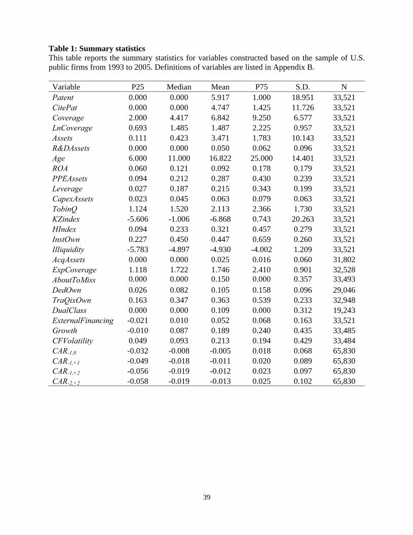
39

Table 1: Summary statistics This table reports the summary statistics for variables constructed based on the sample of U.S. public firms from 1993 to 2005. Definitions of variables are listed in Appendix B. Variable P25 Median Mean P75 S.D. N Patent 0.000 0.000 5.917 1.000 18.951 33,521 CitePat 0.000 0.000 4.747 1.425 11.726 33,521 Coverage 2.000 4.417 6.842 9.250 6.577 33,521 LnCoverage 0.693 1.485 1.487 2.225 0.957 33,521 Assets 0.111 0.423 3.471 1.783 10.143 33,521 R&DAssets 0.000 0.000 0.050 0.062 0.096 33,521 Age 6.000 11.000 16.822 25.000 14.401 33,521 ROA 0.060 0.121 0.092 0.178 0.179 33,521 PPEAssets 0.094 0.212 0.287 0.430 0.239 33,521 Leverage 0.027 0.187 0.215 0.343 0.199 33,521 CapexAssets 0.023 0.045 0.063 0.079 0.063 33,521 TobinQ 1.124 1.520 2.113 2.366 1.730 33,521 KZindex -5.606 -1.006 -6.868 0.743 20.263 33,521 HIndex 0.094 0.233 0.321 0.457 0.279 33,521 InstOwn 0.227 0.450 0.447 0.659 0.260 33,521 Illiquidity -5.783 -4.897 -4.930 -4.002 1.209 33,521 AcqAssets 0.000 0.000 0.025 0.016 0.060 31,802 ExpCoverage 1.118 1.722 1.746 2.410 0.901 32,528 AboutToMiss 0.000 0.000 0.150 0.000 0.357 33,493 DedOwn 0.026 0.082 0.105 0.158 0.096 29,046 TraQixOwn 0.163 0.347 0.363 0.539 0.233 32,948 DualClass 0.000 0.000 0.109 0.000 0.312 19,243 ExternalFinancing -0.021 0.010 0.052 0.068 0.163 33,521 Growth -0.010 0.087 0.189 0.240 0.435 33,485 CFVolatility 0.049 0.093 0.213 0.194 0.429 33,484 CAR-1,0 -0.032 -0.008 -0.005 0.018 0.068 65,830 CAR-1,+1 -0.049 -0.018 -0.011 0.020 0.089 65,830 CAR-1,+2 -0.056 -0.019 -0.012 0.023 0.097 65,830 CAR-2,+2 -0.058 -0.019 -0.013 0.025 0.102 65,830

40

Table 2: Baseline regression of innovation outcomes on analyst coverage This table reports regressions of the innovation outcome variables (number of patents and number of citations per patent) on analyst coverage and other control variables. Definitions of variables are listed in Appendix B. Each regression includes a separate intercept as well as year and firm fixed effects. Robust standard errors clustered by firm are displayed in parentheses. ***, **, and * indicate significance at the 1, 5, and 10 percent levels, respectively.

Panel A Panel B (1) (2) (3) (4) (1) (2) (3) (4) Dep. Var. LnPatentt+1 LnPatentt+2 LnPatentt+3 LnPatentt+5 LnCitePatt+1 LnCitePatt+2 LnCitePatt+3 LnCitePatt+5

LnCoverage -0.028** -0.047*** -0.051*** -0.063*** -0.063*** -0.080*** -0.081*** -0.072*** (0.014) (0.016) (0.018) (0.023) (0.018) (0.019) (0.020) (0.025) LnAssets 0.137*** 0.114*** 0.080*** 0.005 0.127*** 0.081*** 0.033 -0.051 (0.020) (0.022) (0.024) (0.030) (0.025) (0.027) (0.029) (0.035) R&DAssets 0.790*** 0.737*** 0.908*** 0.813*** 1.203*** 1.069*** 0.797*** 0.750*** (0.152) (0.167) (0.192) (0.230) (0.218) (0.222) (0.230) (0.247) LnAge 0.180*** 0.260*** 0.309*** 0.427*** 0.224*** 0.260*** 0.293*** 0.441*** (0.044) (0.050) (0.057) (0.075) (0.058) (0.062) (0.067) (0.080) ROA -0.019 0.187*** 0.362*** 0.329*** 0.211*** 0.367*** 0.306*** 0.306*** (0.058) (0.065) (0.075) (0.088) (0.079) (0.082) (0.090) (0.092) PPEAssets 0.322*** 0.427*** 0.496*** 0.238 0.350*** 0.363*** 0.360** 0.046 (0.087) (0.107) (0.125) (0.154) (0.120) (0.134) (0.143) (0.156) Leverage -0.320*** -0.345*** -0.408*** -0.266** -0.302*** -0.332*** -0.368*** -0.091 (0.064) (0.069) (0.078) (0.105) (0.073) (0.075) (0.082) (0.095) CapexAssets 0.014 0.150 0.233* 0.121 0.087 0.297* 0.355** 0.165 (0.098) (0.113) (0.129) (0.166) (0.148) (0.159) (0.161) (0.172) TobinQ 0.032*** 0.036*** 0.023*** -0.032*** 0.027*** 0.016** 0.005 -0.033*** (0.005) (0.006) (0.006) (0.008) (0.006) (0.006) (0.006) (0.008) KZindex -0.001*** -0.001* -0.001* -0.000 -0.002*** -0.001 -0.002*** -0.002** (0.000) (0.000) (0.000) (0.001) (0.001) (0.000) (0.001) (0.001) HIndex 0.206 0.274* 0.397** 0.666*** 0.372** 0.288 0.264 0.491** (0.135) (0.161) (0.183) (0.248) (0.187) (0.195) (0.201) (0.233)

41

HIndex Squared -0.178 -0.179 -0.201 -0.402* -0.225 -0.114 -0.031 -0.207 (0.121) (0.142) (0.159) (0.214) (0.166) (0.173) (0.179) (0.205) InstOwn 0.067 0.196*** 0.218*** 0.282*** 0.067 0.180** 0.211** 0.308*** (0.058) (0.066) (0.075) (0.092) (0.082) (0.086) (0.095) (0.101) Illiquidity 0.030* 0.076*** 0.098*** 0.104*** 0.059*** 0.077*** 0.069*** 0.074*** (0.016) (0.020) (0.022) (0.028) (0.020) (0.022) (0.024) (0.026) Firm fixed effects Yes Yes Yes Yes Yes Yes Yes Yes Year fixed effects Yes Yes Yes Yes Yes Yes Yes Yes Observations 33,521 30,753 25,860 18,242 33,521 30,753 25,860 18,242 R-squared 0.789 0.751 0.750 0.739 0.666 0.646 0.642 0.624

42

Table 3: DiD test based on propensity score matching: diagnostics and results This table reports diagnostics and results of the DiD tests on how exogenous shocks to analyst coverage (broker closures and mergers) affect firm innovation activities. The sample begins with all firm-years from 1993 to 2005 with non-missing matching variables and non-missing innovation outcome variables during a five-year window (from year -2 to year +2) around the (actual or matched) event year. For broker closures, the treatment firms are those covered by disappearing analysts before the event and whose total analyst coverage goes down by exactly one. For broker mergers, the treatment firms are those covered by both the target and acquirer brokers before the event and for which exactly one of their analysts disappears. The control firms are found by adopting a one-to-three nearest neighbor propensity score matching on a host of observable characteristics including all the independent variables in our baseline regression (as in Table 2), the three-year moving average of innovation variables (patents and citations), growth measures of innovation variables and analyst coverage, a squared term of analyst coverage, and year and Fama-French 49 industry dummies. Panel A presents parameter estimates from the probit model used in estimating the propensity scores for the treatment and control groups. The dependent variable is one if the firm-year belongs to the treatment group and zero otherwise. The Pre-Match column contains the parameter estimates of the probit model estimated on the entire sample, prior to matching. This model is used to generate the propensity scores for matching. The Post-Match column contains the parameter estimates of the probit model estimated on the subsample of matched treatment and unique control firm-years, after matching. Definitions of variables are listed in Appendix B. Both probit regressions in Panel A include a separate intercept as well as year and Fama-French 49 industry fixed effects. Robust standard errors clustered by firm are displayed in parentheses. Panel B reports the distribution of estimated propensity scores for the treatment firm-years, control firm-years, and the difference in estimated propensity scores. Panel C gives the full sample DiD test results. Panel D reports the sub-sample DiD test results based on post-shock number of analysts following the firm. Patent_2yr_avg is firm i’s average number of patents in the two-year window before or after the event year. CitePat_2yr_avg is firm i’s average per-patent citations in the two-year window before or after the event year. Ordinary standard errors are given in parentheses below the mean differences in innovation outcomes and bootstrapped standard errors for the two-sample t-tests with unequal variance are given below the diff-in-diff t-stats. ***, **, and * indicate significance at the 1, 5, and 10 percent levels, respectively.

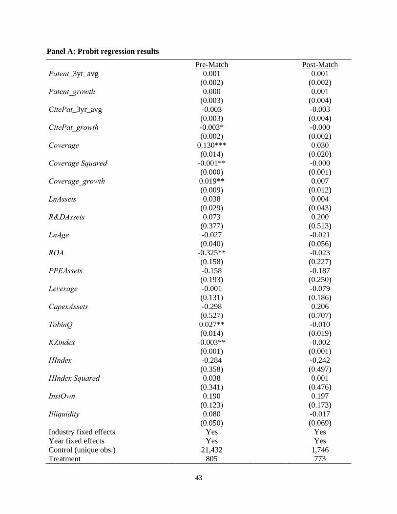
43

Panel A: Probit regression results

Pre-Match Post-MatchPatent_3yr_avg 0.001 0.001 (0.002) (0.002) Patent_growth 0.000 0.001 (0.003) (0.004) CitePat_3yr_avg -0.003 -0.003 (0.003) (0.004) CitePat_growth -0.003* -0.000 (0.002) (0.002) Coverage 0.130*** 0.030 (0.014) (0.020) Coverage Squared -0.001** -0.000 (0.000) (0.001) Coverage_growth 0.019** 0.007 (0.009) (0.012) LnAssets 0.038 0.004 (0.029) (0.043) R&DAssets 0.073 0.200 (0.377) (0.513) LnAge -0.027 -0.021 (0.040) (0.056) ROA -0.325** -0.023 (0.158) (0.227) PPEAssets -0.158 -0.187 (0.193) (0.250) Leverage -0.001 -0.079 (0.131) (0.186) CapexAssets -0.298 0.206 (0.527) (0.707) TobinQ 0.027** -0.010 (0.014) (0.019) KZindex -0.003** -0.002 (0.001) (0.001) HIndex -0.284 -0.242 (0.358) (0.497) HIndex Squared 0.038 0.001 (0.341) (0.476) InstOwn 0.190 0.197 (0.123) (0.173) Illiquidity 0.080 -0.017 (0.050) (0.069) Industry fixed effects Yes Yes Year fixed effects Yes Yes Control (unique obs.) 21,432 1,746 Treatment 805 773

44

Observations 22,237 2,519 Pseudo R-squared 0.374 0.037 Chi-square p-value <0.001 0.297 Panel B: Estimated propensity score distributions

No. of

Unique Obs. Mean SD Min P5 P50 P95 Max

Match No. 1 Difference ––– 0.00 0.00 0.00 0.00 0.00 0.00 0.00 Treatment 773 0.26 0.20 0.00 0.01 0.21 0.66 0.81 Control 757 0.26 0.20 0.00 0.01 0.22 0.64 0.81

Match No. 2 Difference ––– 0.00 0.00 0.00 0.00 0.00 0.01 0.02 Treatment 773 0.26 0.20 0.00 0.01 0.21 0.66 0.81 Control 748 0.27 0.20 0.00 0.01 0.23 0.66 0.79

Match No. 3 Difference ––– 0.00 0.00 0.00 0.00 0.00 0.01 0.02 Treatment 773 0.26 0.20 0.00 0.01 0.21 0.66 0.81 Control 743 0.27 0.20 0.00 0.01 0.23 0.67 0.78

Panel C: Full sample DiD test results (773 treatments)

Mean treatment Difference

(after - before)

Mean control Difference

(after -before)

Mean diff-in-diffs (treat - control)

Z-statistics for diff-in-diffs

Patent_2yr_avg -0.81 -2.84 2.03*** 3.89 (standard error) (1.24) (0.82) (0.52) CitePat_2yr_avg -3.27 -4.31 1.04*** 2.96 (standard error) (0.57) (0.34) (0.35)

45

Panel D: Sub-sample DiD test results Treatments with zero analysts post-shock (478 treatments) Mean treatment

Difference (after - before)

Mean control Difference

(after -before)

Mean diff-in-diffs (treat - control)

Z-statistics for diff-in-diffs

Patent_2yr_avg -1.95 -4.25 2.30*** 3.26 (standard error) (1.19) (1.03) (0.70) CitePat_2yr_avg -3.93 -5.07 1.14** 2.28 (standard error) (0.45) (0.35) (0.50)

Treatments with none-zero analysts post-shock (295 treatments) Mean treatment

Difference (after - before)

Mean control Difference

(after -before)

Mean diff-in-diffs (treat - control)

Z-statistics for diff-in-diffs

Patent_2yr_avg 1.38 -0.03 1.41* 1.85 (standard error) (2.54) (1.48) (0.76) CitePat_2yr_avg -2.17 -2.83 0.66 0.97 (standard error) (1.24) (0.68) (0.68)

46

Table 4: Two-stage least-squares regression with the instrument of expected analyst coverage This table reports the 2SLS regressions of the innovation outcome variables (number of patents and number of citations per patent) on analyst coverage, with expected analyst coverage (ExpCoverage) as the instrumental variable. Panel A reports results for the first-stage regression, which generates the fitted (instrumented) value of LnCoverage for use in second-stage regressions as reported by Panel B and C. Definitions of variables are listed in Appendix B. Each regression includes year and firm fixed effects. Robust standard errors clustered by firm are displayed in parentheses. The R-square in Panel A is a pooled one, and the reported R-squares for second-stage regressions in Panel B and C are within-firm ones. ***, **, and * indicate significance at the 1, 5, and 10 percent levels, respectively.

Panel A

First Stage Panel B

Second Stage Panel C

Second Stage (1) (2) (3) (4) (1) (2) (3) (4) Dep. Var. LnCoverage LnPatentt+1 LnPatentt+2 LnPatentt+3 LnPatentt+5 LnCitePatt+1 LnCitePatt+2 LnCitePatt+3 LnCitePatt+5 ExpCoverage 0.549*** (0.007) LnCoverage -0.040** -0.084*** -0.095*** -0.120*** -0.091*** -0.130*** -0.133*** -0.138*** (instrumented) (0.019) (0.022) (0.026) (0.034) (0.024) (0.026) (0.028) (0.037) LnAssets 0.169*** 0.145*** 0.138*** 0.114*** 0.031 0.141*** 0.111*** 0.073** -0.037 (0.008) (0.019) (0.022) (0.025) (0.032) (0.025) (0.027) (0.030) (0.035) R&DAssets 0.137** 0.843*** 0.843*** 1.153*** 1.050*** 1.323*** 1.170*** 1.087*** 0.950*** (0.068) (0.147) (0.168) (0.200) (0.241) (0.206) (0.218) (0.230) (0.251) LnAge -0.018 0.175*** 0.249*** 0.291*** 0.410*** 0.213*** 0.239*** 0.251*** 0.436*** (0.017) (0.041) (0.048) (0.055) (0.074) (0.054) (0.059) (0.066) (0.078) ROA 0.075*** -0.025 0.172** 0.425*** 0.436*** 0.240*** 0.350*** 0.373*** 0.448*** (0.028) (0.058) (0.068) (0.082) (0.098) (0.078) (0.086) (0.097) (0.098) PPEAssets 0.114*** 0.373*** 0.538*** 0.616*** 0.269* 0.390*** 0.488*** 0.479*** 0.043 (0.044) (0.084) (0.109) (0.129) (0.161) (0.115) (0.135) (0.147) (0.160) Leverage -0.154*** -0.305*** -0.330*** -0.410*** -0.354*** -0.279*** -0.315*** -0.391*** -0.157 (0.026) (0.061) (0.066) (0.075) (0.107) (0.070) (0.074) (0.082) (0.098) CapexAssets 0.231*** -0.009 0.099 0.209 0.149 0.047 0.221 0.334** 0.254 (0.058) (0.095) (0.113) (0.135) (0.178) (0.140) (0.159) (0.165) (0.179)

47

TobinQ 0.009*** 0.032*** 0.039*** 0.024*** -0.037*** 0.025*** 0.018*** 0.004 -0.038*** (0.002) (0.005) (0.006) (0.006) (0.008) (0.006) (0.006) (0.006) (0.007) KZindex -0.000 -0.001*** -0.001 -0.001 0.000 -0.002*** -0.000 -0.002*** -0.002** (0.000) (0.000) (0.000) (0.000) (0.001) (0.000) (0.000) (0.001) (0.001) HIndex 0.124** 0.201 0.290* 0.444** 0.782*** 0.372** 0.308 0.316 0.563** (0.057) (0.130) (0.161) (0.184) (0.248) (0.179) (0.192) (0.199) (0.232) HIndex Squared -0.132*** -0.175 -0.185 -0.220 -0.490** -0.218 -0.119 -0.057 -0.257 (0.051) (0.117) (0.142) (0.160) (0.214) (0.158) (0.170) (0.178) (0.203) InstOwn 0.217*** 0.062 0.219*** 0.259*** 0.367*** 0.077 0.217*** 0.288*** 0.397*** (0.026) (0.055) (0.063) (0.074) (0.091) (0.077) (0.083) (0.093) (0.100) Illiquidity -0.163*** 0.026 0.058*** 0.085*** 0.101*** 0.050** 0.052** 0.054** 0.066** (0.008) (0.016) (0.020) (0.023) (0.028) (0.020) (0.022) (0.024) (0.027) Firm fixed effects Yes Yes Yes Yes Yes Yes Yes Yes Yes Year fixed effects Yes Yes Yes Yes Yes Yes Yes Yes Yes Observations 30,421 30,421 27,069 22,367 15,172 30,421 27,069 22,367 15,172 R-squared 0.619 0.149 0.184 0.201 0.217 0.186 0.216 0.231 0.259

Table 5: Cross-sectional tests for just missing analyst consensus forecasts This table reports the second stage of the 2SLS regressions of the number of patents on instrumented analyst coverage (using ExpCoverage as the instrumental variable), AboutToMiss, and their instrumented interactions. Definitions of variables are listed in Appendix B. Each regression includes a separate intercept as well as year and firm fixed effects. Robust standard errors clustered by firm are displayed in parentheses. The reported R-squares are within-firm ones. ***, **, and * indicate significance at the 1, 5, and 10 percent levels, respectively.

(1) (2) (3) (4) Dep. Var. LnPatentt+1 LnPatentt+2 LnPatentt+3 LnPatentt+5

LnCoverage -0.030* -0.068*** -0.071*** -0.083** (instrumented) (0.018) (0.022) (0.026) (0.033) AboutToMiss * LnCoverage (instrumented)

-0.066*** -0.094*** -0.138*** -0.229*** (0.023) (0.029) (0.034) (0.044)

AboutToMiss 0.085** 0.086** 0.104** 0.194*** (0.034) (0.042) (0.047) (0.064) LnAssets 0.147*** 0.140*** 0.117*** 0.040 (0.019) (0.022) (0.025) (0.031) R&DAssets 0.831*** 0.822*** 1.117*** 1.001*** (0.147) (0.167) (0.197) (0.236) LnAge 0.172*** 0.242*** 0.276*** 0.383*** (0.041) (0.048) (0.055) (0.073) ROA -0.026 0.167** 0.412*** 0.421*** (0.057) (0.067) (0.080) (0.097) PPEAssets 0.369*** 0.535*** 0.617*** 0.283* (0.084) (0.109) (0.128) (0.159) Leverage -0.305*** -0.327*** -0.406*** -0.348*** (0.061) (0.066) (0.076) (0.106) CapexAssets -0.006 0.103 0.208 0.152 (0.095) (0.113) (0.135) (0.179) TobinQ 0.032*** 0.038*** 0.023*** -0.035*** (0.005) (0.006) (0.006) (0.008) KZindex -0.001*** -0.001 -0.001 0.000 (0.000) (0.000) (0.000) (0.001) HIndex 0.197 0.283* 0.430** 0.775*** (0.130) (0.160) (0.183) (0.245) HIndex* HIndex -0.173 -0.182 -0.211 -0.485** (0.117) (0.141) (0.159) (0.213) InstOwn 0.055 0.206*** 0.233*** 0.309*** (0.054) (0.063) (0.073) (0.089) Illiquidity 0.025 0.057*** 0.084*** 0.103*** (0.016) (0.020) (0.023) (0.028) Firm fixed effects Yes Yes Yes Yes Year fixed effects Yes Yes Yes Yes Observations 30,408 27,056 22,352 15,163 R-squared 0.150 0.185 0.205 0.225

49

Table 6: Cross-sectional tests for institutional ownership This table reports the second stage of the 2SLS regressions of the number of patents on instrumented analyst coverage (using ExpCoverage as the instrumental variable), percentage ownership by different types of institutional investors per Bushee (2001) classification (DedOwn and TraQixOwn), and their instrumented interactions. Definitions of variables are listed in Appendix B. Each regression includes a separate intercept as well as year and firm fixed effects. Robust standard errors clustered by firm are displayed in parentheses. The reported R-squares are within-firm ones. ***, **, and * indicate significance at the 1, 5, and 10 percent levels, respectively.

(1) (2) (3) (4) Dep. Var. LnPatentt+1 LnPatentt+2 LnPatentt+3 LnPatentt+5 LnCoverage -0.035* -0.080*** -0.100*** -0.135*** (instrumented) (0.019) (0.018) (0.026) (0.035) DedOwn* LnCoverage 0.332*** 0.330*** 0.018 0.231* (instrumented) (0.072) (0.073) (0.100) (0.118) TraQixOwn * LnCoverage -0.047 -0.092** -0.057 -0.213** (instrumented) (0.046) (0.038) (0.060) (0.084) DedOwn 0.032 -0.006 -0.065 -0.137 (0.076) (0.069) (0.098) (0.120) TraQixOwn 0.053 0.230*** 0.309*** 0.433*** (0.051) (0.044) (0.071) (0.086) LnAssets 0.148*** 0.141*** 0.115*** 0.035 (0.019) (0.015) (0.025) (0.032) R&DAssets 0.852*** 0.859*** 1.148*** 1.052*** (0.147) (0.126) (0.199) (0.242) LnAge 0.166*** 0.245*** 0.295*** 0.412*** (0.041) (0.027) (0.055) (0.074) ROA -0.027 0.172*** 0.417*** 0.425*** (0.057) (0.051) (0.081) (0.098) PPEAssets 0.375*** 0.525*** 0.597*** 0.229 (0.084) (0.076) (0.128) (0.160) Leverage -0.306*** -0.329*** -0.403*** -0.343*** (0.061) (0.044) (0.075) (0.107) CapexAssets -0.031 0.073 0.191 0.136 (0.095) (0.117) (0.135) (0.178) TobinQ 0.032*** 0.039*** 0.025*** -0.035*** (0.005) (0.004) (0.006) (0.008) KZindex -0.001*** -0.000 -0.001 0.000 (0.000) (0.000) (0.000) (0.001) HIndex 0.198 0.285*** 0.439** 0.786*** (0.129) (0.103) (0.183) (0.247) HIndex Squared -0.175 -0.185** -0.220 -0.503** (0.116) (0.092) (0.159) (0.213) Illiquidity 0.021 0.054*** 0.086*** 0.098*** (0.016) (0.014) (0.023) (0.028) Firm fixed effects Yes Yes Yes Yes Year fixed effects Yes Yes Yes Yes Observations 30,467 27,110 22,401 15,191 R-squared 0.151 0.186 0.202 0.219

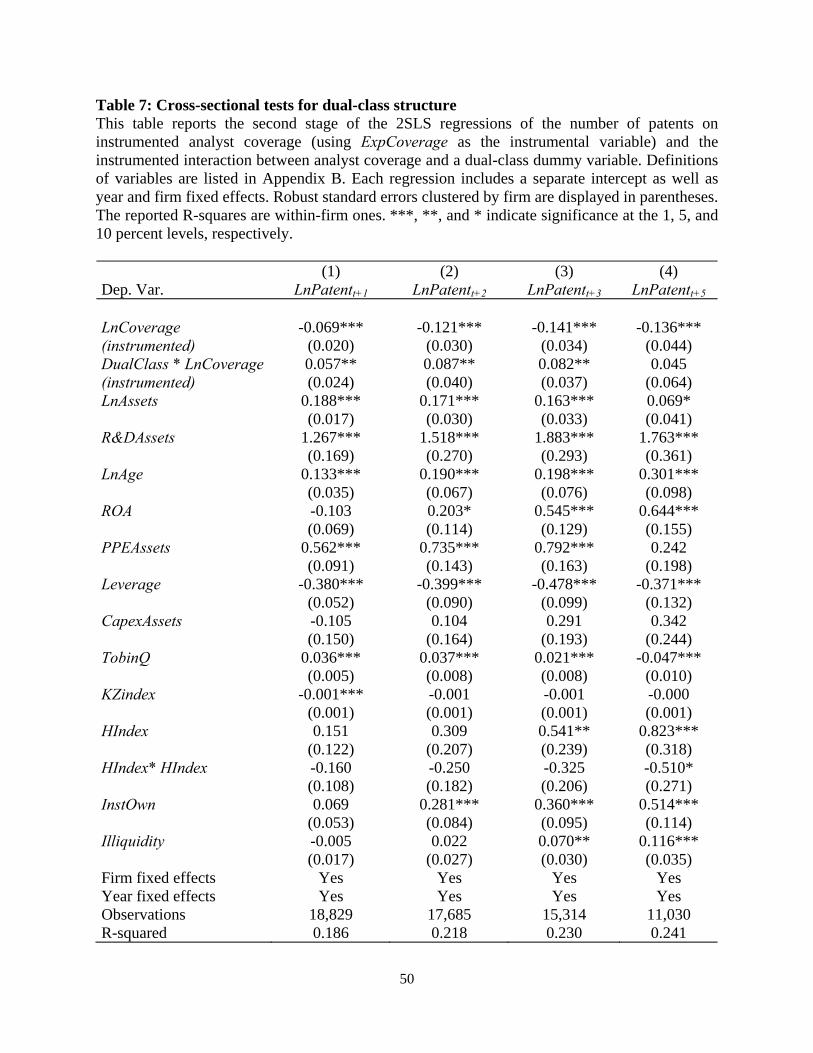
50

Table 7: Cross-sectional tests for dual-class structure This table reports the second stage of the 2SLS regressions of the number of patents on instrumented analyst coverage (using ExpCoverage as the instrumental variable) and the instrumented interaction between analyst coverage and a dual-class dummy variable. Definitions of variables are listed in Appendix B. Each regression includes a separate intercept as well as year and firm fixed effects. Robust standard errors clustered by firm are displayed in parentheses. The reported R-squares are within-firm ones. ***, **, and * indicate significance at the 1, 5, and 10 percent levels, respectively.

(1) (2) (3) (4) Dep. Var. LnPatentt+1 LnPatentt+2 LnPatentt+3 LnPatentt+5 LnCoverage -0.069*** -0.121*** -0.141*** -0.136*** (instrumented) (0.020) (0.030) (0.034) (0.044) DualClass * LnCoverage 0.057** 0.087** 0.082** 0.045 (instrumented) (0.024) (0.040) (0.037) (0.064) LnAssets 0.188*** 0.171*** 0.163*** 0.069* (0.017) (0.030) (0.033) (0.041) R&DAssets 1.267*** 1.518*** 1.883*** 1.763*** (0.169) (0.270) (0.293) (0.361) LnAge 0.133*** 0.190*** 0.198*** 0.301*** (0.035) (0.067) (0.076) (0.098) ROA -0.103 0.203* 0.545*** 0.644*** (0.069) (0.114) (0.129) (0.155) PPEAssets 0.562*** 0.735*** 0.792*** 0.242 (0.091) (0.143) (0.163) (0.198) Leverage -0.380*** -0.399*** -0.478*** -0.371*** (0.052) (0.090) (0.099) (0.132) CapexAssets -0.105 0.104 0.291 0.342 (0.150) (0.164) (0.193) (0.244) TobinQ 0.036*** 0.037*** 0.021*** -0.047*** (0.005) (0.008) (0.008) (0.010) KZindex -0.001*** -0.001 -0.001 -0.000 (0.001) (0.001) (0.001) (0.001) HIndex 0.151 0.309 0.541** 0.823*** (0.122) (0.207) (0.239) (0.318) HIndex* HIndex -0.160 -0.250 -0.325 -0.510* (0.108) (0.182) (0.206) (0.271) InstOwn 0.069 0.281*** 0.360*** 0.514*** (0.053) (0.084) (0.095) (0.114) Illiquidity -0.005 0.022 0.070** 0.116*** (0.017) (0.027) (0.030) (0.035) Firm fixed effects Yes Yes Yes Yes Year fixed effects Yes Yes Yes Yes Observations 18,829 17,685 15,314 11,030 R-squared 0.186 0.218 0.230 0.241

51

Table 8: Regressions of CARs around earnings announcements on analyst coverage This table reports regressions of the cumulative market model abnormal returns (CARs) over different windows around quarterly earnings announcement on analyst coverage when the reported earnings fall short of the consensus forecast outstanding at the earnings announcement date. LnCoverage is the natural logarithm of one plus the average number of analysts following the firm over the three months prior to the earnings announcement date. The other explanatory variables include: forecast error (ForecastError), which is the difference between the reported quarterly earnings and the consensus analyst forecast (the median analyst forecast over the three months prior to the earnings announcement date), deflated by the stock price 30 days prior to the announcement; the price-earnings ratio based on the stock price 30 days prior to the announcement (PEratio); the natural logarithm of the quarterly market value of equity (LnMV); the quarterly Tobin’s Q (TobinQ); the average of annual sales growth over the prior three years (SalesGrowth); the quarterly dividend yield (DivYield); and the average market-adjusted stock return for the 12 months prior to the announcement (Runup). Each regression includes a separate intercept as well as year, quarter, and firm fixed effects. Robust standard errors clustered by firm are displayed in parentheses. ***, **, and * indicate significance at the 1, 5, and 10 percent levels, respectively. (1) (2) (3) (4) Dep. Var. CAR-1,0 CAR-1,+1 CAR-1,+2 CAR-2,+2 LnCoverage -0.002** -0.006*** -0.004*** -0.003** (0.001) (0.001) (0.001) (0.002) ForecastError 0.109*** 0.207*** 0.235*** 0.256*** (0.013) (0.018) (0.019) (0.021) PEratio -0.000* -0.000** -0.000*** -0.000*** (0.000) (0.000) (0.000) (0.000) LnMV -0.009*** -0.013*** -0.015*** -0.017*** (0.001) (0.001) (0.001) (0.001) TobinQ -0.000 -0.000 -0.000 -0.000 (0.001) (0.001) (0.001) (0.001) SalesGrowth -0.001 0.000 0.000 0.000 (0.001) (0.001) (0.001) (0.001) DivYield 0.091 0.185 0.212 0.174 (0.147) (0.193) (0.219) (0.225) Runup -0.108*** -0.198*** -0.266*** -0.300*** (0.012) (0.017) (0.018) (0.020) InstOwn -0.009*** -0.017*** -0.016*** -0.022*** (0.003) (0.004) (0.005) (0.005) Firm fixed effects Yes Yes Yes Yes Year fixed effects Yes Yes Yes Yes Quarter fixed effects Yes Yes Yes Yes Observations 65,830 65,830 65,831 65,831 R-squared 0.176 0.196 0.197 0.198

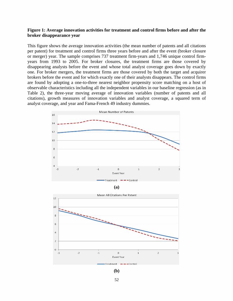
52

Figure 1: Average innovation activities for treatment and control firms before and after the broker disappearance year This figure shows the average innovation activities (the mean number of patents and all citations per patent) for treatment and control firms three years before and after the event (broker closure or merger) year. The sample comprises 737 treatment firm-years and 1,746 unique control firm-years from 1993 to 2005. For broker closures, the treatment firms are those covered by disappearing analysts before the event and whose total analyst coverage goes down by exactly one. For broker mergers, the treatment firms are those covered by both the target and acquirer brokers before the event and for which exactly one of their analysts disappears. The control firms are found by adopting a one-to-three nearest neighbor propensity score matching on a host of observable characteristics including all the independent variables in our baseline regression (as in Table 2), the three-year moving average of innovation variables (number of patents and all citations), growth measures of innovation variables and analyst coverage, a squared term of analyst coverage, and year and Fama-French 49 industry dummies.

(a)

(b)