The dark matter interpretation of the 3.5-keV line isinconsistent with blank-sky observations

Christopher Dessert,1 Nicholas L. Rodd,2,3 Benjamin R. Safdi1

1Leinweber Center for Theoretical Physics, Department of Physics,University of Michigan, Ann Arbor, MI 48109, USA

2Berkeley Center for Theoretical Physics,University of California, Berkeley, CA 94720, USA

3Theoretical Physics Group, Lawrence Berkeley National Laboratory,Berkeley, CA 94720, USA

Observations of nearby galaxies and galaxy clusters have reported an unex-

pected X-ray emission line around 3.5 kilo–electron volts (keV). Proposals to

explain this line include decaying dark matter—in particular, that the decay

of sterile neutrinos with a mass around 7 keV could match the available data.

If this interpretation is correct, the 3.5 keV line should also be emitted by dark

matter in the halo of the Milky Way. We used more than 30 megaseconds

of XMM-Newton (X-ray Multi-Mirror Mission) blank-sky observations to test

this hypothesis, finding no evidence of the 3.5-keV line emission from the Milky

Way halo. We set an upper limit on the decay rate of dark matter in this mass

range, which is inconsistent with the possibility that the 3.5-keV line originates

from dark matter decay.

A plethora of cosmological and astrophysical measurements indicate that dark matter (DM)

exists and makes up∼80% of the matter in the Universe, but its microscopic nature is unknown.

1

arX

iv:1

812.

0697

6v3

[as

tro-

ph.C

O]

1 M

ar 2

021

If DM consists of particles that can decay into ordinary matter, the decay process may produce

photons that are detectable with X-ray telescopes. Some DM models, such as sterile neutrino

DM, predict such X-ray emission lines [1]. If the sterile neutrinos exist with a mass-energy

of a few kilo–electron volts, they may explain the observed abundance of DM [2, 3, 4]. The

detection of an unidentified X-ray line (UXL) around 3.5 keV in a stacked sample of nearby

galaxy clusters [5] and an independent detection in one of those clusters and a galaxy [6] have

been interpreted as evidence for DM decay [7]. Other less-exotic explanations have also been

proposed, such as emission lines of potassium or argon, from hot gas within the clusters [8], or

charge-exchange lines from interactions of the hot intracluster plasmas and cold gas clouds [9,

10].

The 3.5-keV UXL (hereafter just UXL) has been confirmed by several groups using different

astrophysical targets and telescopes. These include observations of the Perseus cluster using the

Chandra [5] and Suzaku [11] telescopes, observations of the Galactic Center of the Milky Way

with XMM-Newton (X-ray Multi-Mirror Mission) [12], and observations of the diffuse Milky

Way halo with Chandra deep-field data [13]. Several non-detections of the UXL have also

been reported [14, 15, 16, 17, 18]. It is possible for a decaying DM model to be consistent

with both the positive detections and negative results. Fig. 1 shows the existing detections and

upper limits for the UXL, in the plane of sterile neutrino DM mass ms and sterile-active mixing

parameter sin2(2θ), which characterizes (and linearly scales with) the decay rate of the sterile

neutrino DM state [19].

We seek to constrain the DM decay rate in the mass range relevant for the UXL by using

XMM-Newton blank-sky observations (BSOs). Our analysis utilizes ∼103 BSOs, which we

define as observations away from large X-ray emitting regions, for a total of 30.6 Ms of exposure

time. We focus on the line signal predicted from DM decay within the Milky Way, which should

be present at every point in the sky. The sensitivity of this technique can be estimated in the

2

6.7 6.8 6.9 7.0 7.1 7.2 7.3 7.4ms [keV]

10−12

10−11

10−10

10−9

sin

2 (2θ)

1

2

3 4

5

6

7

8

9

10

95% limit (this work)

mean expected

1σ/2σ containment

Figure 1: Our upper limits on sterile neutrino decay. The one-sided 95% upper limit onthe sterile neutrino DM mixing parameter sin2(2θ) as a function of the DM mass ms from ouranalysis of XMM-Newton BSOs (black squares). We compare with the expected sensitivityfrom the Asimov procedure (1σ shown in green and 2σ in yellow), and previous constraints(gray lines) and parameters required for DM decay explanations of previous UXL detections(3σ in dark gray, 2σ in gray, and 1σ in light gray). We also show several existing detections(labelled 1 to 5) and constraints (6 to 10) [7].

3

limit of large counts, in other words, detected photons. Then the test statistic (TS) in favor of

detection of DM decay (related to the significance σ ∼√

TS), scales as TS ∼ S2/B, where S

is the number of signal photons from DM decay and B is the number of background photons.

The number of signal photons expected from a given location in the sky is proportional to the

product of the decay rate of DM and the integrated column density of DM along the line of

sight, which is quantified by the D factor, D =∫ds ρDM(s) where ρDM is the DM density and

s is the line-of-sight distance.

We use these scalings to estimate the expected sensitivity of a BSO analysis, given the

previous UXL observations. For example, the UXL has been detected with a 320-ks observation

of the Perseus cluster using the XMM-Newton Metal Oxide Semiconductor (MOS) camera at

roughly the 4σ level (TS ∼ 16) [5]. The background X-ray flux from Perseus is much higher

than that for the BSOs, typically by a factor of 50. Averaged over the field of view of XMM-

Newton, theD factor of the Perseus cluster isDPers ∼ 3×1028 keVcm−2, which is approximately

the same asDBSO, theD factor within the Milky Way halo for observations∼45 away from the

Galactic Center. We calculated both D factors assuming a Navarro-Frenk-White (NFW) DM

profile [20]. Although the signal power should therefore be the same between Perseus and the

BSO, we expect the same sensitivity to the UXL with a 6 ks BSO observation—assuming a DM

origin—because the BSO background is expected to be lower than that of Perseus. Our analysis

below uses ∼ 30 Ms of BSO exposure time, which implies that the UXL would be seen with a

TS ∼ 105, corresponding to a detection significance of > 100σ, if it is caused by decaying DM

with the same properties as that in the Perseus cluster.

We analyzed all publicly-available archival XMM-Newton observations that pass a set of

quality cuts. For our fiducial analysis, we first restrict to the observations used to those between

5 and 45 of the Galactic Center. Within this region there are 1492 observations, with 4303 total

exposures, for ∼86 Ms of exposure time. These observations are distributed quite uniformly

4

through our fiducial region, although there is a bias towards the Galactic plane. There are

more exposures than observations because each of the European Photon Imaging Cameras

charged coupled devices (CCDs) onboard XMM-Newton [two MOS and one positive-negative

(PN)] [21, 22] records a separate exposure, and each camera may have multiple exposures

in a single observation if the data taking was interrupted. For each observation we process

and reduce the data using the standard tools for extended emission [19]. In addition to the

photon-count data, we also extract the quiescent particle background (QPB). The QPB is an

instrumental background caused by high-energy particles interacting with the detector, rather

than true photon counts. The magnitude of the QPB contribution is estimated from parts of the

instrument that are shielded from incident X-rays; we refer to this as the QPB data.

We then perform a background-only analysis of each of the exposures to determine proper-

ties that are used for further selection. We calculate the QPB contribution and the astrophysical

flux over the energy range of 2.85 to 4.2 keV. The QPB rate is estimated from the QPB data,

whereas the astrophysical flux is measured using the likelihood analysis described below. We

rescale the astrophysical flux measured in the restricted energy range to a wider energy range of

2 to 10 keV by assuming a power-law spectrum of dN/dE ∼ E−1.5 where N is the photon flux

and E is energy. The cosmic X-ray background has a 2 to 10 keV intensity of I2−10 ≈ 2×10−11

erg cm−2 s−1 deg−2 [23, 24]. In our fiducial analysis we remove exposures with I2−10 > 10−10

erg cm−2 s−1 deg−2 to avoid including exposures with either extended emission or flux from

unresolved point sources. Approximately 58% of the exposures pass this cut, whereas ∼13%

of the exposures have I2−10 < 3× 10−11 erg cm−2 s−1 deg−2. Because the individual exposures

are in the background-dominated regime and the signal we are searching for is restricted to a

narrow energy range, even a clearly detectable DM line would have no effect on this selec-

tion criterion. We further remove exposures with anomalously high QPB rates; for our fiducial

analysis, we keep the 68% of exposures with the lowest QPB rates. We apply this criterion sep-

5

arately to the MOS and PN exposures. Lastly, we remove exposures with < 1 ks of exposure

time, because these exposures do not substantially improve our sensitivity and the associated

low photon counts reduce the reliability of the background estimates. After these cuts, we

are left with ∼30.6 Ms of exposure time distributed between 1397 exposures and 752 distinct

observations.

We analyze the ensemble of exposures for evidence of the UXL by using a joint likelihood

procedure. Individual exposures are not stacked. To evaluate the UXL hypothesis for a given

ms, we first construct profile likelihoods for the individual exposures as functions of the DM-

induced line flux F . The X-ray counts are analyzed with a Poisson likelihood, from the number

of counts in each energy channel. The associated model is a combination of the DM-induced

flux represented by an X-ray line broadened by the detector response and two independent

power laws for the background astrophysical emission and the instrumental QPB, where the

normalization and spectral indices of each power law are free parameters. This same QPB

power-law contribution is also fitted to the estimated QPB data using a Gaussian likelihood.

Both datasets are restricted to the energy range ms/2±0.25 keV, which was chosen to be wider

than the energy resolution of the detector (∼0.1 keV) but small enough that our power-law

background models are valid over the whole energy range.

The two likelihoods for the X-ray counts and the QPB estimate are then combined, providing

a likelihood that, for a given ms, is a function of five parameters: the DM-induced line flux F

and the normalization factors and spectral indices of the astrophysical and QPB power laws.

The last four of these are treated as nuisance parameters; that is, we maximize the individual

likelihoods over the valid ranges of these parameters. Each dataset was therefore reduced to

a profile likelihood as a function of F . This flux can be converted to a lifetime and, hence,

sin2(2θ) [1, 19], once the D factor for this region of the sky is known. In our fiducial analysis

we compute the D factors by assuming that the DM density profile of the Milky Way is an

6

NFW profile with a 20 kpc scale radius. We normalize the density profile, assuming a local DM

density of 0.4 GeVcm−3 [25], and take the distance between the Sun and the Galactic Center to

be 8.13 kpc [26].

Joining the resulting likelihoods associated with each exposure yields the final joint likeli-

hood that is a function of only sin2(2θ) for a given ms. This likelihood is then used to calculate

the one-sided 95% confidence limit on the mixing angle and to search for evidence for the

UXL using the discovery TS, which is defined as twice the log-likelihood difference between

the maximum likelihood and the likelihood at the null hypothesis [assuming the likelihood is

maximized at a positive value of sin2(2θ)]. For statistical consistency, we must include negative

values of sin2(2θ) in the profile likelihood, which correspond to under-fluctuations of the data.

To calibrate our expectation for the sensitivity under the null hypothesis, we construct the

68 and 95% expectations for the limit using the Asimov procedure [27]. The Asimov procedure

requires a model for the data under the null hypothesis; we compute this model by performing

the likelihood fits described above under the null hypothesis [sin2(2θ) = 0]. We use this to

set one-sided power-constrained limits [28]. The measured limit is not allowed to go below

the 68% containment region for the expected limit, so as to prevent setting tighter limits than

expected because of downward statistical fluctuations.

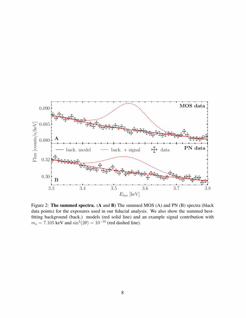
In Fig. 2, we show the summed spectra over all exposures included in the analysis for the

MOS and PN data separately. We emphasize that we do not use the summed spectra for our

fiducial data analysis; instead we use the joint likelihood procedure described above. However,

the summed spectra are shown for illustrative purposes. We also show the summed best-fitting

background models. Because our full model has independent astrophysical and QPB power-

law models for each exposure, these curves are not single power laws but sums over 2794

independent power-laws. The summed data closely match the summed background models.

Fig. 2 also shows the expected signal for ms = 7.105 keV and sin2(2θ) = 10−10, which are

7

0.080

0.085

0.090

Flu

x[c

ount

s/s/

keV

]

MOS data

A

3.3 3.4 3.5 3.6 3.7 3.8Eline [keV]

0.30

0.32

cou

nts/

s/ke

V

PN data

B

back. model back. + signal data

Figure 2: The summed spectra. (A and B) The summed MOS (A) and PN (B) spectra (blackdata points) for the exposures used in our fiducial analysis. We also show the summed best-fitting background (back.) models (red solid line) and an example signal contribution withms = 7.105 keV and sin2(2θ) = 10−10 (red dashed line).

8

values we chose to be in the middle of the parameter space for explaining the observed UXL

(Fig. 1). Fig. 2 shows that this model is inconsistent with the data.

Our fiducial one-sided power-constrained 95% upper limit is shown in Fig. 1 along with

mean, 1σ, and 2σ expectations under the null hypothesis. The upper limit is consistent with the

expectation values and strongly disfavors the decaying DM explanation of the UXL. Our results

disagree with the parameters required to explain the previous UXL observations as decaying

DM by over an order of magnitude in sin2(2θ). In Fig. 3, we show the TS for decaying DM as

a function of DM mass, with the 1 and 2σ expectations under the null hypothesis; we find no

evidence for decaying DM.

Fig. 3 shows the TS for the joint-likelihood analysis over the ensemble of exposures. How-

ever, we can also calculate a TS for decaying DM from each individual exposure. Under the

null hypothesis, Wilks’ theorem states that the distribution of TSs from the individual exposures

should asymptotically follow a χ2 distribution. In the inset of Fig. 3, we show the histogram of

the number of exposures that are found for a given TS, for our reference mass of ms = 7.105

keV. The distribution matches the expectation under the null hypothesis. We also performed a

Kolmogorov-Smirnov test comparing the observed TSs with the expected one-sided χ2 distri-

bution, and found a P value of 0.77, which indicates that the TS data is consistent with the null

hypothesis.

Although Fig. 3 shows that our results appear to be consistent with the expected statistical

variability, there remains the possibility that systematic effects such as un-modeled instrumental

lines could conspire to hide a real line. We test for such systematics in Fig. S9 by analyzing

the data from the individual cameras separately [19], in Fig. S14 by explicitly allowing for

extra possible instrumental lines in the background model [19], and in Figs. S16 and S17 by

looking at the data in sub-regions increasingly far away from the Galactic Center [19]. Ac-

counting for these possible systematics in a data-driven way may weaken our limits to as much

9

6.7 6.8 6.9 7.0 7.1 7.2 7.3 7.4

ms [keV]

0

1

2

3

4

5

TS

A

0 5 10

TS

10−1

100

101

102dN

obs/d

(TS

)

B

Figure 3: No evidence for the decaying DM interpretation of the UXL. (A) The TS for theUXL as a function of the DM mass ms from the joint likelihood analysis. The black curveshows the result from the data analysis, whereas the green and yellow shaded regions indicatethe 1σ and 2σ expectations, respectively, under the null hypothesis. (B) A histogram of theTSs from the individual exposures, with vertical error bars from Poisson counting statistics andhorizontal error bars bracketing the histogram bin ranges.

10

as sin2(2θ) < 2 × 10−11 (Fig. S17, Reg. 4), which still strongly rules out the decaying DM

interpretation of the UXL. We also analyze the summed X-ray count data shown in Fig. 2 di-

rectly [19], and found, again, that the decaying DM interpretation of the UXL was excluded

(see Fig. S18).

We have analyzed ∼30 Ms of XMM-Newton BSOs for evidence of DM decay in the energy

range of 3.35 to 3.7 keV. We found no evidence for DM decay. Our analysis rules out the de-

caying DM interpretation of the previously observed 3.5 keV UXL because our results exclude

the required decay rate by more than an order of magnitude.

References

[1] P. B. Pal, L. Wolfenstein, Phys. Rev. D 25, 766 (1982).

[2] S. Dodelson, L. M. Widrow, Phys. Rev. Lett. 72, 17 (1994).

[3] X.-D. Shi, G. M. Fuller, Phys. Rev. Lett. 82, 2832 (1999).

[4] A. Kusenko, Phys. Rev. Lett. 97, 241301 (2006).

[5] E. Bulbul, et al., Astrophys. J. 789, 13 (2014).

[6] A. Boyarsky, O. Ruchayskiy, D. Iakubovskyi, J. Franse, Phys. Rev. Lett. 113, 251301

(2014).

[7] K. N. Abazajian, Phys. Rept. 711-712, 1 (2017).

[8] T. E. Jeltema, S. Profumo, Mon. Not. Roy. Astron. Soc. 450, 2143 (2015).

[9] L. Gu, et al., Astron. Astrophys. 584, L11 (2015).

[10] C. Shah, et al., Astrophys. J. 833, 52 (2016).

11

[11] O. Urban, et al., Mon. Not. Roy. Astron. Soc. 451, 2447 (2015).

[12] A. Boyarsky, J. Franse, D. Iakubovskyi, O. Ruchayskiy, Phys. Rev. Lett. 115, 161301

(2015).

[13] N. Cappelluti, et al., Astrophys. J. 854, 179 (2018).

[14] S. Horiuchi, et al., Phys. Rev. D89, 025017 (2014).

[15] D. Malyshev, A. Neronov, D. Eckert, Phys. Rev. D90, 103506 (2014).

[16] M. E. Anderson, E. Churazov, J. N. Bregman, Mon. Not. Roy. Astron. Soc. 452, 3905

(2015).

[17] T. Tamura, R. Iizuka, Y. Maeda, K. Mitsuda, N. Y. Yamasaki, Publ. Astron. Soc. Jap. 67,

23 (2015).

[18] F. A. Aharonian, et al., Astrophys. J. 837, L15 (2017).

[19] Materials and methods are available as supplementary materials.

[20] J. F. Navarro, C. S. Frenk, S. D. M. White, Astrophys. J. 462, 563 (1996).

[21] M. J. L. Turner, et al., Astron. Astrophys. 365, L27 (2001).

[22] L. Struder, et al., Astron. Astrophys. 365, L18 (2001).

[23] D. H. Lumb, R. S. Warwick, M. Page, A. De Luca, Astron. Astrophys. 389, 93 (2002).

[24] A. Moretti, AIP Conf. Proc. 1126, 223 (2009).

[25] R. Catena, P. Ullio, J. Cosmol. Astropart. Phys. 1008, 004 (2010).

[26] R. Abuter, et al., Astron. Astrophys. 615, L15 (2018).

12

[27] G. Cowan, K. Cranmer, E. Gross, O. Vitells, Eur. Phys. J. C71, 1554 (2011).

[28] G. Cowan, K. Cranmer, E. Gross, O. Vitells, https://arxiv.org/abs/1007.1727 (2011).

[29] C. Dessert, N. L. Rodd, B. R. Safdi, nickrodd/XMM-DM: XMM-DM

https://doi.org/10.5281/zenodo.3669387 (2020).

[30] ”Users Guide to the XMM-Newton Science Analysis System”, Issue 14.0, 2018 (ESA:

XMM-Newton SOC).

[31] M. Cicoli, J. P. Conlon, M. C. D. Marsh, M. Rummel, Phys. Rev. D90, 023540 (2014).

[32] J. P. Conlon, F. V. Day, J. Cosmol. Astropart. Phys. 1411, 033 (2014).

[33] Kuntz, K. D., Snowden, S. L., Astron. Astrophys. 478, 575 (2008).

[34] W. A. Rolke, A. M. Lopez, J. Conrad, Nucl. Instrum. Meth. A551, 493 (2005).

[35] F. James, M. Roos, Comput. Phys. Commun. 10, 343 (1975).

[36] A. Burkert, IAU Symp. 171, 175 (1996).

[37] P. Salucci, A. Burkert, Astrophys. J. 537, L9 (2000).

[38] J. F. Navarro, C. S. Frenk, S. D. M. White, Astrophys. J. 490, 493 (1997).

[39] P. F. Hopkins, et al., Mon. Not. Roy. Astron. Soc. 480, 800 (2018).

[40] F. Nesti, P. Salucci, J. Cosmol. Astropart. Phys. 1307, 016 (2013).

[41] L. Struder, et al., Nuclear Instruments and Methods in Physics Research A 512, 386

(2003).

[42] O. Ruchayskiy, et al., Mon. Not. Roy. Astron. Soc. 460, 1390 (2016).

13

[43] A. Boyarsky, D. Iakubovskyi, O. Ruchayskiy, D. Savchenko,

https://arxiv.org/abs/1812.10488 (2018).

Acknowledgments

We thank S. Mishra-Sharma for collaboration in the early stages of this work, K. Abazajian,

J. Beacom, A. Boyarsky, E. Bulbul, D. Finkbeiner, J. Kopp, K. Perez, S. Profumo, J. Thaler,

and C. Weniger for useful discussions and comments on the draft. We further thank K. Abaza-

jian for preliminary discussions of this topic, and the members of the XMM-Newton Helpdesk

for assistance with the data reduction process. We downloaded the observations used in this

work from the XMM archive. We provide a full list of exposures used in our fiducial analysis,

data-reduction software, our analysis code, and the numerical data plotted in the figures at [29].

CD and BRS were supported by the Department of Energy Early Career Grant DE-SC0019225.

NLR is supported by the Miller Institute for Basic Research in Science at the University of Cal-

ifornia, Berkeley. Computational resources and services were provided by Advanced Research

Computing at the University of Michigan, Ann Arbor.

14

Supplementary Materials forThe dark matter interpretation of the 3.5-keV line is

inconsistent with blank-sky observationsChristopher Dessert, Nicholas L. Rodd, Benjamin R. Safdi

1 Materials and Methods

1.1 Data Reduction

The data products were downloaded from the XMM-Newton Science Archive and processed into

the X-ray spectra and QPB flux estimates used in the main text. This process is applied to each

exposure individually. We have applied our data reduction pipeline to all 6,350 observations

within 90 of the Galactic Center, collected by XMM-Newton up to 2018 September 5 (the

instrument collected a total of 12,044 observations in that time). The data reduction process uses

the XMM-Newton Extended Source Analysis Software (ESAS) package for modeling extended

objects and the diffuse X-ray backgrounds. The ESAS package is part of the XMM-Newton

Science Analysis System (SAS) [30]; we used version 17.0.

After selecting an observation, we obtain summary information for this dataset and its as-

sociated exposures. The Calibration Index File (CIF) is generated using the task cifbuild,

which locates the Current Calibration File (CCF). The CCF provides information about the state

of the detector at observation time; for example, it supplies the location of bad pixels on the de-

tector. Next, the task odfingest is used to generate the Observation Data Files (ODF), which

contains uncalibrated summary files in addition to general information on the observation in-

cluding data quality records. The relevant science exposures for each observation ID to use for

data reduction are determined from the Pipeline Processing Subsystem summary file. Only PN

exposures in submodes Full Frame and Extended Full Frame were chosen to ensure

an accurate estimate of the instrumental Quiescent Particle Background (QPB).

1

From this information, a set of filtered events is then created for both MOS and PN cameras

for each available science exposure. The PN pipeline is as follows. The task epchain is first

used to generate an event list. The list of out-of-time events, which are events recorded while

the CCD is being read out, is generated with epchain withoutoftime=true. After

obtaining the list of events, the task pn-filter is called to record only those events that

occurred during a good time interval (GTI). This task calls the SAS routine espfilt to filter

the light-curves for periods of soft proton (SP) contamination. An observation affected by SP

will typically have a count rate histogram with a peak at the unaffected rate, and a long tail due

to the contamination. espfilt establishes thresholds at ±1.5σ of the count rate distribution,

and then creates a GTI file containing the time intervals where the data is contained within

those limits. The MOS pipeline is analogous to that for PN, requiring the tasks emchain and

mos-filter.

Now that the data has been cleaned, we identify regions of the dataset we wish to mask.

The routine cheese is applied to search for any point sources in the field of view for the

energy range 3 − 4 keV. The resulting mask is then used to exclude these sources from further

analysis. Applying this mask also removes the necessity of a pile-up correction, as for extended

source analyses this is only a concern near point sources. In addition, MOS CCDs flagged as

anomalous are disregarded. For example, a suspected micrometeorite impact caused the loss of

MOS1 CCD6 on 2005 March 12, and a similar event caused the loss of MOS1 CCD3 on 2012

December 11. These CCDs are excluded from analysis for observations made after these dates.

With the cleaned data masked, the final step is the production of the spectra and QPB data.

For the PN and MOS cameras this is achieved with the tasks pn-spectra and mos-spectra

respectively. These tasks use the filtered event files to create the photon-count data, the QPB

data, the Ancillary Response File (ARF), and the source count weighted Redistribution Matrix

File (RMF), for the masked region but otherwise the full field of view (FOV). The ARF and

2

RMF account for the detector response, and will be described in more detail in the following

subsection.

1.2 Data Analysis

For a given exposure, we model the observed number of X-rays as originating from a combi-

nation of instrumental effects and conventional astrophysical sources, which we consider back-

grounds, and a putative DM decay line as our signal hypothesis. The DM in the Milky Way

is sufficiently non-relativistic (v ∼ 10−3 in natural units where v is velocity of the DM) that

we treat the decay signal as a zero-width line at an energy ms/2. The line-width generated

by the finite velocity dispersion of DM within the Milky Way is small compared to the energy

resolution of the detector. The flux of this line in counts cm−2s−1sr−1keV−1, averaged over the

full region of interest (ROI) for this observation, is given by

dΦ

dE=dΦpp

dE×D , (S1)

where the particle physics and D-factor contributions are given by

dΦpp

dE=

Γ

4πms

δ(E −ms/2) , D =

∫ds ρDM(s,Ω) . (S2)

Above, Γ = τ−1 is the DM decay rate (the inverse of the DM lifetime τ ), s is an integration

variable along the line-of-sight, and ρDM is the Milky Way DM distribution, which will be

discussed further below. For our searches for DM decay in the ambient MW, we may computeD

using any angular position within the ROI, and use this as an estimate for the average D factor.

This is because variations in the line-of-sight integral through the Milky Way halo are negligible

(at most∼2% for the regions we consider) over the small XMM-Newton field-of-view. However,

if the DM density varies over the scale of the ROI, as is the case when considering extragalactic

sources such as galaxy clusters, then theD-factor needs to be averaged over the ROI, accounting

3

for the vignetting of the instrument. Note the D-factor here is the Decay analogue of the J-

factor, which is used for DM annihilation. For the specific case of sterile-neutrino DM, the

decay rate can be related to the mixing angle between active and sterile neutrinos, θ, as [1]

Γ = 1.361× 10−29 s−1(

sin2 2θ

10−7

)( ms

1 keV

)5. (S3)

This expression is valid for a Majorana neutrino, for a Dirac neutrino it is a factor of 2 smaller.

For each observation, we only included the contribution from the MW halo DM column

density. Each region will also include a large column density from extragalactic DM. We can

neglect the extragalactic contribution because an extragalactic line emitted over cosmological

distances will be smeared out by redshifting, and the resulting smooth emission will be more

than an order of magnitude smaller than the line from the MW halo.

We have concentrated on sterile neutrino DM, but our results apply to any model of decaying

DM which produces an X-ray line. Alternate models for the 3.5 keV UXL have been proposed,

however, that involve the decay of DM into an ultralight axion-like particle, which converts to

photons within the galactic and/or cluster magnetic fields [31]. Our results do not directly apply

to these models because the spatial morphology of the signal is a convolution of the DM density

distribution and the magnetic field distribution. Estimating the size of the effect [32] indicates

that our results also constrain this DM.

By restricting our attention to relatively blank regions of the sky and a narrow energy range,

we reduce the number of backgrounds that need to be considered. As discussed in the main

text, we model the contributions to the X-ray counts using a power-law instrumental QPB rate

and a power-law astrophysical spectrum, which may also describe the soft proton background

if present [33]. In principle, the soft proton background an unfolded power-law that has not

been passed through the instrument response, however we find that including such an additional

model has minimal impact on our results. Physical astrophysical emission may be present

4

within the ROIs from the cosmic X-ray background, extended emission regions, or unresolved

populations of Galactic sources. We model the QPB spectrum using a power-law in counts,

while the astrophysical emission is modeled by a power-law in flux. A flux power-law is,

in principle, not directly equivalent to a counts power-law because of the energy-dependent

detector response. However, over the narrow energy ranges we consider the distinction is small.

Still, for consistency we model the spectra in these different ways.

Given the signal and astrophysical background models, we calculate the predicted num-

ber of model counts in each of the camera channels. Let us define S(E, θephys) in units of

counts cm−2s−1sr−1keV−1, as the signal and astrophysical background spectrum, as a func-

tion of energy E. Within this expression, the index e is used to enumerate the different ex-

posures. The parameters θephys denote the astrophysical background parameters and the signal

parameters for the given exposure e. The signal parameters can be separated out by writing

θephys = ms, Γ, θeB, where θeB are the background astrophysical power-law parameters. The

QPB is not included here but will be incorporated separately, as described below. By using Γ

we keep our discussion appropriate for a general decaying DM scenario, but the analysis can

immediately be specialized to the sterile neutrino scenario using equation (S3). For the decay-

ing DM hypothesis the DM parameters do not vary throughout the Milky Way or over time,

and thus must be identical across exposures, so they do not carry an index e. The background

parameters do vary between exposures and thus must be treated independently. Explicitly, the

expected flux can be written as follows:

S(E, θephys) =ΓD

4πms

δ(E −ms/2) + Aeastro

(E

1 keV

)neastro

. (S4)

To compare this predicted spectrum to the observed number of X-rays in counts, we use

forward modeling to incorporate the instrument response. The predicted number of counts in a

5

given energy bin indexed by i is given by

µei,phys(θephys) = te∆Ωe

∫dE ′RMFei (E

′) ARFe(E ′)S(E ′, θephys) , (S5)

where te is the observation time for the given exposure in s, ∆Ωe is the angular area of the

ROI, the ARF provides the effective area of the detector as a function of energy in cm2, and the

dimensionless RMF accounts for the energy resolution and detector gain effects. All of these

detector quantities vary between exposures and so carry an explicit e index. We now add to

equation (S5) the contribution from the QPB rate as a power law in reconstructed (rather than

true) energy

µei,QPB(θeQPB) = AeQPB × EneQPB

i , (S6)

where θeQPB = AeQPB, neQPB are the model parameters defining the power-law. The separate

treatment for the QPB arises as its flux is not folded with the detector response.

For the given exposure we now have the total predicted model counts µei in each energy bin

as a function of the model parameters θe = θephys, θeQPB:

µei (θe) = µei,phys(θ

ephys) + µei,QPB(θeQPB) . (S7)

The data collected in this exposure can be identically binned, such that we can represent the

X-ray dataset for each exposure by a set of integers deX-ray = kei , where explicitly kei is the

number of X-rays in energy bin i for this exposure. With the data and model in identical forms,

we can now compare the two by constructing a joint likelihood over all energy bins as follows

LeX-ray(deX-ray|θe) =∏i

µei (θe)k

ei e−µ

ei (θ

e)

kei !. (S8)

The above likelihood accounts for the X-ray data collected during a given exposure, but

there is additional information collected by the cameras that we incorporate into our model.

This arises in the form of an estimate for the QPB background during the given exposure, as

6

determined from pixels on the CCD that were shielded and therefore unexposed to direct X-

rays. The ESAS tools provide this information as the mean and standard deviation on the (non-

integer) QPB counts in each energy bin, which we denote by λei,QPB and σei,QPB respectively.

We then construct a Gaussian likelihood for the QPB dataset deQPB = λei,QPB, σei,QPB as

LeQPB(deQPB|θeQPB) =∏i

1

σei,QPB

√2π

exp

[−(µei,QPB(θeQPB)− λei,QPB)2

2(σei,QPB)2

]. (S9)

To account for both the X-ray and QPB data simultaneously, we form the joint likelihood as

Le(de|ms,Γ, θeB) = LeX-ray(deX-ray|θephys)× LeQPB(deQPB|θeQPB) , (S10)

where de = deX-ray, deQPB and where θeB denotes the four model parameters that describe the

background astrophysical power-law and the power-law QPB model.

In a similar manner we can construct likelihoods for each exposure, recalling that the signal

parameters will not vary between them. We therefore remove these background parameters at

the level of individual exposures, using the standard frequentist technique of profiling. At fixed

ms we construct the profile likelihood as a function of Γ [34]. The profile likelihood is given by

Le(de|ms,Γ) = Le(de|ms,Γ, θeB) , (S11)

with θeB denoting the value of each of the background parameters that maximizes the likelihood

for the specific values of ms and Γ under consideration. This technique does not involve fixing

the background to its value under the null hypothesis or the signal hypothesis. Instead, we

determine a new value for θeB for each value of Γ considered, at fixed ms using minuit [35].

We construct a profile likelihood for each exposure, leaving a likelihood depending only on

the DM parameters. The information from each of these exposures can then be combined into

the joint likelihood, which depends on the entire dataset d = de:

L(d|ms,Γ) =∏e

Le(de|ms,Γ) . (S12)

7

We reiterate that the signal parameters do not vary between exposures.

Using the likelihood in equation (S12) we perform hypothesis testing between a signal

model containing a DM decay line at fixed ms and the null hypothesis without the DM line.

Following frequentist standards, we will quantify the significance of any excess using a test

statistic (TS) for discovery

TS(ms) =

2[lnL(d|ms, Γ)− lnL(d|ms,Γ = 0)

]Γ ≥ 0 ,

0 Γ < 0 .(S13)

Here Γ is the value of Γ that maximizes the likelihood at fixedms, and asymptotically TS(ms) =

σ2, where σ is the significance of the excess. We may also construct a test statistic appropri-

ate for establishing one-sided limits on Γ for a fixed ms. Note that Γ is physically constrained

(Γ ≥ 0), though for consistency we must consider negative values of Γ as well, so we define [27]

q(ms,Γ) =

2[lnL(d|ms, Γ)− lnL(d|ms,Γ)

]Γ ≤ Γ ,

0 Γ > Γ .(S14)

This statistic then allows us to determine the one-sided 95% limit on the decay rate Γ95% by

solving q(ms,Γ95%) = 2.71. We also power-constrain the limits, to avoid setting stronger limits

than expected due to statistical fluctuations [28], as discussed in the main text. To obtain the

expected value for q(ms,Γ), we apply the Asimov procedure [27] to the null hypothesis. The

interpretation of the square root of the discovery TS as being the significance of the line and the

precise TS threshold used to calculate the one-sided 95% limit rely on the TS in equation (S13)

following a one-sided χ2 distribution under the null hypothesis. This is justified by the fact that

our photon statistics are sufficient to invoke Wilks’ theorem.

2 Supplementary Text

In this section, we provide extended results for the fiducial analysis presented in the main text

and test variations to the procedure. This section is organized as follows. First, we subject our

8

fiducial analysis to a key statistical test by injecting a synthetic signal into the data. Then, we

present results from individual exposures and determine which observations contribute most to

our limits. In the following section, we consider how our limits depend on assumptions for the

DM profile of the Milky Way. In the final sub-section we explore how our sensitivity varies for

different selection criteria on the exposures.

2.1 Synthetic Signal

The limit on decaying DM, shown in Fig. 1, is tighter than in previous studies. We therefore

subject our analysis to test that it is statistically meaningful. For example, it is possible that

systematic effects cause the limit to appear stronger than it should be and that a real signal, if

present, would be excluded by our analysis. To test this possibility, we add a synthetic signal to

the real data and verify that our limit does not exclude the signal that we inject.

We perform this analysis for our fiducial selection criterion described in the main text. The

results of the test, for three different assumed DM masses, are shown in Fig. S1. That figure

shows the value of the mixing angle for the synthetic signal injected into the data, θinj, and

the mixing angle recovered by our analysis, θrec. The 95% one-sided limits are computed as

the injected signal strength is varied. The limits never fall below the true value of the injected

signal for any of the mass points shown. The mean, 1 and 2σ expectations for the 95% one-

sided limit under the signal hypothesis were computed from the Asimov procedure [27]. Our

limits are consistent with the real data being a realization of the null hypothesis and the only

signal contribution comes from that which we inject.

There is no inconsistency in that the lower 2σ band for the 95% one-sided limit falls below

the injected value. This is expected because the one-sided 95% limit and the 2σ bands for the

95% limit have different statistical interpretations, because the 2σ band is a 2-sided interval

while the one-sided 95% limit is a statement about a one-sided interval. Figure S1 also shows

9

10−12 10−11 10−10

sin2(2θinj)

10−12

10−11

10−10

sin

2 (2θ r

ec)

mχ = 6.8 keV

(A)

10−12 10−11 10−10

sin2(2θinj)

10−12

10−11

10−10

sin

2 (2θ r

ec)

mχ = 7.0 keV

(B)

10−12 10−11 10−10

sin2(2θinj)

10−12

10−11

10−10

sin

2 (2θ r

ec)

mχ = 7.3 keV

(C)

Figure S1: Results of the synthetic signal test. We inject an artificial DM signal to the data,with mixing angle sin2(2θinj) as indicated on the x-axes, and recover values sin2(2θrec), shownon the y-axes. In (A), we show the results for 6.8 keV; (B), for 7.0 keV; (C), for 7.3 keV. Thered curves show the power-constrained 95% one-sided upper limits that we find on the analysisof the hybrid datasets, consisting of the real data plus the synthetic signal. The bands show themean (black), 1σ (green) and 2σ (yellow) expectations for the 95% one-sided upper limit. Theinjected signal strength is never excluded, as indicated by the red line never dropping below thedashed black diagonal line.

10

that the lower 2σ bands flatten at low injected mixing angles. This is because we are showing

power-constrained limits [28], and those values reach the constraints.

We also test the effect of assuming the wrong DM density profile. We consider how our lim-

its change for different assumed DM profiles below. Here, we address the question of whether

the evidence for a real DM-induced line may be obscured if an incorrect DM profile is used in

the profile likelihood analysis. We follow the same procedure described above to construct a

hybrid dataset consisting of the real data and a synthetic signal at ms = 7.0 keV. That synthetic

signal is constructed assuming our canonical NFW DM profile. We then analyze the synthetic

data assuming the DM profile follows the alternative Burkert DM profile [36, 37]. That profile

is an extreme departure from the NFW DM profile, in that it has a roughly 9 kpc core. The

difference between the spatial morphologies of the NFW profile and the Burkert profile encap-

sulate the largest mismatch between the DM profiles we test in this work and the real profile of

the Milky Way.

In Fig. S2 we show the resulting TS in favor of DM as a function of the synthetic injected

mixing angle, for an analysis that assumes the NFW DM profile and one that assumes the

Burkert DM profile, with the NFW DM profile injected. The two TS curves are extremely

similar, so we conclude that a real signal is not going undetected because we do not have the

correct DM density profile. In both cases the D-factor does not change appreciably between

different exposures in our region of interest. In both cases the TS at sin2(2θinj) ≈ 10−10 is

∼103, meaning that at this signal strength a DM-induced line would have been detected at

approximately 30σ.

If the DM profile used in the analysis is not correct then the limit will be systematically

biased. However, Fig. S2 shows the true limit, constructed with the correct DM profile, may be

obtained by rescaling the limit obtained with an incorrect DM profile by the appropriate ratio of

mean D-factors, where the means are constructed from the ensemble of exposures used in the

11

joint-likelihood analysis.

As an additional cross-check, below we compute the limit on the DM-induced line in re-

gions consisting of narrow annuli centered around the Galactic Center. For all the DM profiles

considered, these annuli are small enough that the DM density does not change appreciably

between exposures in these subregions.

2.2 Individual Exposures

Our fiducial result relied on the construction of the joint likelihood over 1,397 independent

exposures. We now consider the sensitivity of the most constraining individual exposures, and

their individual properties. We begin by describing how the individual exposures in our fiducial

analysis are distributed.

2.2.1 Spatial Distribution of exposures

Fig. S3 shows the spatial distribution of the exposures included in the fiducial analysis about

the Galactic Center. In cases where there are multiple exposures at the same location, we have

only shown the highest exposure case. This can be compared with Fig. S4, which shows the TS

at three different mass points for the exposures illustrated in Fig. S3. The high-TS exposures do

not correlate with distance from the Galactic Center and appear randomly distributed about the

region.

12

10−12 10−11

sin2(2θinj)

100

101

102

103

TS

NFW Profile

Burkert Profile

Figure S2: The effects of a different DM profile. As in Fig. S1, we add a fake DM signalto the real data, with mixing angle sin2(2θinj) as indicated on the x-axis. Here we have fixedms = 7.0 keV. We show the TS assuming the NFW DM profile (red), which was used in theproduction of the synthetic signal, and the Burkert profile (black dashed) with a 9 kpc core. TheTS is almost insensitive to the DM profile assumed.

−40−2002040

` [degrees]

−40

−20

0

20

40

b[d

egre

es]

0.0

0.5

1.0

1.5

2.0

2.5lo

g 10(

exp

osu

re/k

s)

Figure S3: A map of the exposure times. Exposure times for the exposures included in thefiducial analysis on a map of galactic coordinates, where l is longitude and b is latitude. In caseswhere multiple exposures occur at the same position, we only show the longest exposure time.

13

2.2.2 Goodness of fit for individual exposures

We quantify the goodness of fit for an individual exposure through the δχ2 per degree of free-

dom. In calculating δχ2 we only include the X-ray count data, and we also take the degrees of

freedom to be the number of data points minus two to account for the two degrees of freedom

in the astrophysical power-law. We assume that the QPB model parameters are already fixed by

the QPB data, for the purpose of counting model parameters. There are typically ∼100 energy

bins in the 0.5 keV energy window around the putative line energy considered in the analysis.

The exact number of energy bins varies slightly as a function of the line energy. We present

results for ms = 7.1 keV, though the results at other masses are similar. In this case, there are

100 energy bins included in the MOS analyses and 97 in the PN analyses. Thus, we take 98

(95) degrees of freedom for the MOS (PN) exposures.

In Fig. S5 we show the distribution of δχ2 per degree of freedom (DOF) over all of the

MOS and PN exposures in the fiducial analysis. The vertical error bars show the 1σ Poisson

counting uncertainties. The data histograms are consistent with expectations under the null

hypothesis. Under the null hypothesis these distributions should follow the χ2 distribution with

the appropriate number of degrees of freedom.

2.2.3 Top 10 Exposures

We show the limits obtained from the top 10 exposures individually in Fig. S6. These exposures

are listed in Table S1, ranked in order of the strongest predicted limit under the null hypothesis,

from the Asimov analysis at ms = 7.0 keV. None of the top 10 exposures were proposed to

search for extended emission. These ten observations were all looking at specific astrophysical

sources, which we mask in our analysis.

Fig. S6A shows the one-sided 95% power-constrained limits obtained from these exposures.

Many of these top 10 exposures are themselves strong enough to independently disfavor the de-

14

−40−2002040` [degrees]

−40

−20

0

20

40

b[d

egre

es]

mχ = 6.88 keV

A

−40−2002040` [degrees]

−40

−20

0

20

40

b[d

egre

es]

B

mχ = 7.11 keV

−40−2002040` [degrees]

−40

−20

0

20

40

b[d

egre

es]

mχ = 7.23 keV

C

012345678

TS

Figure S4: Maps of the maximum TSs. The maximum TSs for the individual exposuresillustrated in Fig. S3 at three different mass points 6.88 keV (A), 7.11 keV (B), and 7.28 keV(C). The high-TS exposures appear randomly distributed about the region.

15

Table S1: The 10 most constraining XMM-Newton exposures in the fiducial analysis. Theexposures are ranked by their predicted limits under the null hypothesis at ms = 7.0 keVfrom the Asimov analysis. The “Identifier” column denotes the specific exposure within anobservation. LMXRB stands for “low-mass X-ray binary.”

ObservationID

Camera IdentifierExposure

[ks]l [deg] b [deg] Target Type

0653550301 PN S003 63.2 5.1 -6.2 Quiescent Novae

0203750101 PN S003 33.7 -2.8 -4.9LMXRB Black

Hole

0152750101 PN S001 30.1 1.6 7.1 Dark Cloud

0203750101 MOS2 S002 43.4 -2.8 -4.9LMXRB Black

Hole

0781760101 PN S003 46.0 -2.7 -6.1 LMXRB Burster

0761090301 PN S003 95.2 -8.7 17.0 B2III Star

0206610101 PN S003 35.4 -2.9 7.0 Dark Cloud

0412601501 MOS2 S002 90.2 -1.4 -17.2 Neutron Star

0727760301 MOS2 S003 67.9 -1.4 -17.2 Neutron Star

0761090301 MOS2 S002 107.4 -8.7 17.0 B2III Star

16

caying DM interpretation of the UXL. None of these exposures show evidence for an UXL.

This is illustrated in Fig. S6B, which shows the TSs as a function of mass for the top 10 expo-

sures. There is only one exposure whose TS exceeds the 2σ expectation. This, however, is not

surprising, considering that there are 10 independent exposures and each exposure has roughly

three independent mass points across the mass range considered.

2.2.4 Profile Likelihood for the Top Exposure

We describe in detail our most constraining exposure, observation ID 0653550301 in Table S1.

Our goal is to illustrate the profile likelihood procedure at the level of the individual exposures.

The X-ray count and QPB data for this exposure are shown Fig. S7A. The data are shown

over a 0.5 keV energy range centered around the example line energy of 3.55 keV. The figure

also shows the best-fitting QPB and astrophysical models under the assumption of no signal.

The models match the data within the statistical noise, which can be quantified by calculat-

ing the χ2 per degree of freedom: χ2/DOF ≈ 1.016. We then construct the profile likeli-

hood for the putative line signal at 3.55 keV. In constructing the profile likelihood we re-fit

for the best-fitting nuisance parameters for each value of the line signal strength, as is man-

dated by the profile likelihood procedure. The resulting profile likelihood is shown in Fig. S7B.

We show the profile likelihood as twice the difference in log likelihood with the convention

2∆ lnL = 2[lnL(sin2(2θ)) − lnL(sin2(2θ))], where θ is the value of θ that maximizes the

likelihood. Note that the best-fitting mixing angle is slightly negative in this case. To convert

from counts to flux to sin2(2θ) within this exposure and for ms = 3.55 keV, we use the fol-

lowing properties. First, the average D-factor within this region for the fiducial NFW profile is

9.15× 1028 keV/cm2. Second, the channel bin widths are 0.015 keV wide because this is a PN

exposure. And third, a spectral value of 1 count/cm2/s/sr/keV at 3.55 keV produces, on average,

∼22 counts, distributed across a ∼0.2 keV-wide window in channels about 3.55 keV, due to the

17

0.6 0.8 1.0 1.2 1.4δχ2/DOF

0

20

40

60

80

100

Nob

s

MOS

(A)

0.6 0.8 1.0 1.2 1.4δχ2/DOF

0

10

20

30

40

50

60

Nob

s

PN

(B)

Figure S5: The distribution of δχ2/DOF for the MOS (A) and PN (B) exposures consideredin our fiducial analysis for ms = 7.1 keV. The number of degrees of freedom is 98 (95) forthe MOS (PN) exposures. Under the null hypothesis, these distributions should follow theappropriate χ2-distributions, which are shown in dashed red. The vertical error bars on theblack data points are the 1σ Poisson counting uncertainties, while the horizontal error barsshow the bin ranges. The observed data are consistent with the null hypothesis model.

6.7 6.8 6.9 7.0 7.1 7.2 7.3 7.4ms [keV]

10−12

10−11

10−10

10−9

sin

2 (2θ)

1

2

3 4

5

6

7

8

9

10

(A)

6.7 6.8 6.9 7.0 7.1 7.2 7.3 7.4

mχ [keV]

0

1

2

3

4

5

6

TS

(B)

Figure S6: Limits from individual exposures. (A) The one-sided power-constrained 95%limits (red) from the 10 most constraining exposures, which are listed in Table S1. The shadedregions and pre-existing constraints are as labeled in Fig. 1. (B) The maximum TSs (red) forthe 10 exposures. The distribution of TSs observed is consistent with the null hypothesis. Thegreen and yellow regions indicate 1σ and 2σ detections, respectively.

18

energy resolution of the camera.

We compare the 2 − 10 keV intensity and the QPB rate for this exposure to sets of cuts on

our fiducial analysis. Under the null hypothesis, we infer F2−10 ≈ 3.47×10−11 erg/cm2/s/deg2

and a QPB rate that is in the lower 57% percentile, with a rate of ∼0.127 QPB counts/s.

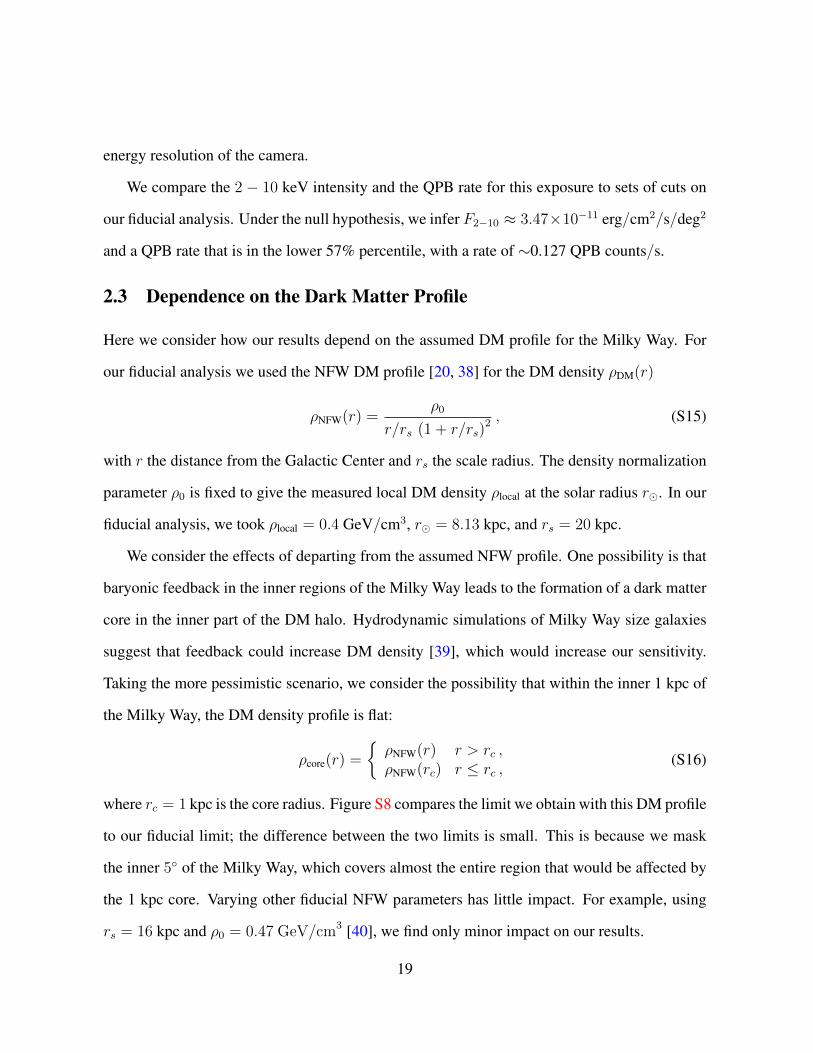
2.3 Dependence on the Dark Matter Profile

Here we consider how our results depend on the assumed DM profile for the Milky Way. For

our fiducial analysis we used the NFW DM profile [20, 38] for the DM density ρDM(r)

ρNFW(r) =ρ0

r/rs (1 + r/rs)2 , (S15)

with r the distance from the Galactic Center and rs the scale radius. The density normalization

parameter ρ0 is fixed to give the measured local DM density ρlocal at the solar radius r. In our

fiducial analysis, we took ρlocal = 0.4 GeV/cm3, r = 8.13 kpc, and rs = 20 kpc.

We consider the effects of departing from the assumed NFW profile. One possibility is that

baryonic feedback in the inner regions of the Milky Way leads to the formation of a dark matter

core in the inner part of the DM halo. Hydrodynamic simulations of Milky Way size galaxies

suggest that feedback could increase DM density [39], which would increase our sensitivity.

Taking the more pessimistic scenario, we consider the possibility that within the inner 1 kpc of

the Milky Way, the DM density profile is flat:

ρcore(r) =

ρNFW(r) r > rc ,ρNFW(rc) r ≤ rc ,

(S16)

where rc = 1 kpc is the core radius. Figure S8 compares the limit we obtain with this DM profile

to our fiducial limit; the difference between the two limits is small. This is because we mask

the inner 5 of the Milky Way, which covers almost the entire region that would be affected by

the 1 kpc core. Varying other fiducial NFW parameters has little impact. For example, using

rs = 16 kpc and ρ0 = 0.47 GeV/cm3 [40], we find only minor impact on our results.

19

3.3 3.4 3.5 3.6 3.7 3.8

E [keV]

0

25

50

75

100

125

150

175

200

cou

nts

QPB model

astro model

astro+QPB model

X-ray counts

QPB counts

(A)

−1.0 −0.5 0.0 0.5 1.0

sin2(2θ)× 1010

0

2

4

6

8

10

12

2∆lnL

(B)

Figure S7: Results for our most constraining exposure. (A) An example spectrum obtainedfrom the PN camera of observation ID 0653550301, our most constraining exposure, as listed inTable S1. In addition to the data (black circles) we show the best-fitting QPB and astrophysicalmodels (red line and dashed black line respectively), under the assumption of no UXL. Theenergy range shown corresponds to that in our fiducial analysis, and the individual energy binsare 0.015 keV wide. (B) The profile likelihood for the strength of the 3.55 keV signal for thedataset shown on the left, in terms of the mixing angle.

6.7 6.8 6.9 7.0 7.1 7.2 7.3 7.4ms [keV]

10−12

10−11

10−10

10−9

sin

2 (2θ)

1

2

3 4

5

6

7

8

9

10

NFW profile

NFW w/ 1 kpc core

Burkert profile

Nesti+Salucci

Figure S8: Limits with different DM density profiles. The parameter space from Fig. 2,compared to our limits for different assumptions about the DM density profile. In additon tothe fiducial NFW profile (solid red), we consider the NFW profile with a 1 kpc core (dot-shortdashed red), an NFW with rs = 16 kpc and ρ0 = 0.47 GeV/cm3 [40] (dot-long dashed red),and the Burkert profile with a 9 kpc core (dashed red). See text for details.

20

We also consider the Burkert DM profile [36, 37]:

ρBurk(r) =ρ0

(1 + r/rc)(1 + (r/rc)2), (S17)

where rc is the core radius and again ρ0 is fixed by matching ρlocal. To be conservative, we take

the core radius to be rc = 9 kpc [40], which effectively corresponds to coring the DM density

profile within the solar radius. While there is no evidence that this density profile describes our

own Milky Way, we consider it the largest plausible deviation from the NFW profile. The limit

is also shown in Fig. S8. Even with such an extreme DM profile we still find that the best-fitting

parameters for DM to explain the UXL remain inconsistent with our results. Changing between

the NFW and Burkert profiles has a small effect on the limit, as within our fiducial region the

difference between the D-factors computed between the two profiles is relatively small.

2.4 MOS and PN Independent Analyses

We analyze the data from the MOS and PN cameras separately to test for systematic issues in

the cameras. Because these are different detectors, we also expect their instrumental systematic

uncertainties (such as effective area uncertainties and possible instrumental lines) to also be

largely independent. In Fig. S9 we show the limits and TS distributions from independent

analyses of the MOS and PN datasets, as compared to the joint (fiducial) analysis. Neither

dataset shows evidence for DM decay, and both constrain the decaying DM interpretation of the

UXL. A low-significance feature (TS ∼1) is seen in both datasets at ms ∼ 6.8 keV. While this

feature could be a statistical fluctuation, it is also possible that it is due to a common systematic,

such as a feature in the background emission, that affects both analyses. Nevertheless, this

feature is not distinguishable from statistical fluctuations.

21

2.5 Variations to Selection Criteria

We tested how our limits change when we vary the selection criteria for the exposures used to

produce the joint likelihood. We summarize the various combinations of the criterion that we

consider in Table S2. The region of interest extends from rmin to rmax from the Galactic Center,

with the Galactic plane masked at |b|min. We include all exposures with 2-10 keV intensity

less than Imax2−10. Similarly, we include exposures with QPB rates in the lower Fmax

QPB percentile,

separately determined for MOS and PN exposures. For two of the analyses, we mask either the

northern or southern hemispheres as well.

In Fig. S10 we show the limits obtained with the criteria given in Table S2. Our main

conclusion – that the decaying DM interpretation of the UXL is inconsistent with our results –

is insensitive to these variations in the selection criterion.

2.6 Energy binning

In our fiducial analysis we used the default energy binning recommended by the XMM-Newton

analysis software. The PN forward modeling matrix uses 15 eV input energy bins, for physical

flux, in our energy range of interest and outputs predicted detector counts in 5 eV output energy

channels. The MOS forward modeling matrix maps 5 eV input energy bins to 5 eV output

energy channels. Because the output energy channel widths are much smaller than the detector

energy resolution, our results should not depend on the energy binning. We test this by down-

binning the detector responses to lower energy resolutions.

As a demonstration, we focus on the individual PN observation with observation ID 0653550301

used in Fig. S7. In our fiducial analysis there are 97 output energy channels across the 0.5 keV

energy window of the analysis. However, the energy resolution of the PN camera, which is

captured by the forward modeling procedure that we use, is around 0.1 keV. Thus we expect

that down-binning the forward modeling matrix to∼5 energy channels, each of 0.1 keV, should

22

6.7 6.8 6.9 7.0 7.1 7.2 7.3 7.4ms [keV]

10−12

10−11

10−10

10−9

sin

2 (2θ)

1

2

3 4

5

6

7

8

9

10

fiducial

MOS

PN

(A)

6.7 6.8 6.9 7.0 7.1 7.2 7.3 7.4ms [keV]

0

1

2

3

4

5

TS

fiducial

MOS

PN

(B)

Figure S9: Exploring the results from individual cameras. Variations to the limit (A) and TS(B) arising from performing independent analyses on the MOS (solid black) and PN (dashedblack) datasets, to test for possible systematic effects present in one camera but not in the other.These can be compared to the fiducial results (red). We find that both limits are independentlyinconsistent with the decaying DM interpretation of the UXL.

6.7 6.8 6.9 7.0 7.1 7.2 7.3 7.4ms [keV]

10−12

10−11

10−10

10−9

sin

2 (2θ)

1

2

3 4

5

6

7

8

9

10

low QPB

high QPB

t > 10 ks

fiducial

F low2−10

F high2−10

(A)

6.7 6.8 6.9 7.0 7.1 7.2 7.3 7.4ms [keV]

10−12

10−11

10−10

10−9

sin

2 (2θ)

1

2

3 4

5

6

7

8

9

10

north

south

|b| ≥ 1.5

fiducial

|r| ≥ 10

|r| ≤ 60

(B)

Figure S10: Variations to the limits arising from different selection criteria that determinewhich exposures are included in the joint likelihood. In (A) we vary the cuts on the exposureswhile in (B) we vary the regions considered. The various criteria are summarized in Table S2.In all cases the decaying DM origin of the UXL is inconsistent with the resulting limits.

23

Table S2: The different selection criteria that we test in Fig. S10. These are variations to thecuts we have chosen in our fiducial analysis.

rmin

[deg]rmax

[deg]|b|min

[deg]

Imax2−10

[erg/cm2/s/deg2]Fmax

QPB[%]

Exposure[Ms]

other

fiducial 5 45 0 10−10 68 30.6 -

r ≥ 10 10 45 0 10−10 68 27.9 -

r ≤ 60 5 60 0 10−10 68 56.9 -

b ≥ 1.5 5 45 1.5 10−10 68 24.8 -

north 5 45 0 10−10 68 12.5 mask b < 0

south 5 45 0 10−10 68 18.1 mask b > 0

F low2−10 5 45 0 5× 10−11 68 18.8 -

F high2−10 5 45 0 5× 10−10 68 35.7 -

low QPB 5 45 0 10−10 16 6.3 -

high QPB 5 45 0 10−10 95 45.6 -

t > 10 ks 5 45 0 10−10 68 28.2require

te > 10 ks

24

have little effect on the resulting profile likelihood for the putative UXL. This is demonstrated

in Fig. S11, which shows the X-ray and QPB data down-binned to 5∼0.1 keV energy channels,

with the best-fitting astrophysical power-law and QPB power-law models from the joint likeli-

hood fit using the down-binned data. The profile likelihood for the UXL at 3.55 keV is shown

compared to the fiducial profile likelihood. The differences between the two profile likelihoods

are small, with the fiducial profile likelihood being slightly more sensitive. This is because the

0.1 keV energy bins are at the limit of the detector energy resolution.

Down-binning further leads to a large decrease in sensitivity, since the UXL then becomes

degenerate with the other (nuisance) model parameters. As an extreme example, we show the

single-bin profile likelihood in Fig. S11B, where we have adopted a single output energy bin

with a width of 0.15 keV centered around 3.55 keV. Because we are using a single energy bin,

the UXL model parameter is completely degenerate with the model parameters describing the

QPB and X-ray power-laws. As such, it would not be possible to find evidence for a UXL with

this analysis, but the limit obtained is maximally conservative. The limit is sin2(2θ) . 2.8 ×

10−10 at 95% confidence, so any larger value of sin2(2θ) would overproduce the entire observed

X-ray data in this energy bin, without any modeling. The profile likelihoods in Fig. S11 show

that the fiducial and 5-bin likelihoods are symmetric and quadratic about their minimum, the 1-

bin profile likelihood is zero at low sin2(2θ) and then rises steeply at high sin2(2θ). Any model

flux from the UXL that is below the observed X-ray counts can be compensated by the nuisance

models (astrophysical and QPB models), which implies that all such models will fit the data

equally well. As sin2(2θ) becomes arbitrarily negative the other models are allowed to become

arbitrarily large to compensate. However, as sin2(2θ) increases and the UXL model flux begins

to surpass the observed data counts, the flux from the nuisance parameters is driven to zero (the

nuisance astrophysical and QPB models are restricted to positive flux). Comparing the 1-bin

profile likelihood to the fiducial profile likelihood, we see that modeling the astrophysical and

25

3.3 3.4 3.5 3.6 3.7 3.8

E [keV]

0.0

0.1

0.2

0.3

0.4

0.5

cou

nts

/s

/ke

V

astro + QPB model

astro model

QPB model

X-ray counts

QPB counts

(A)

−1 0 1 2 3sin2(2θ) ×10−10

0

2

4

6

8

10

12

2∆lo

gL

fiducial

5 bins

1 bin

(B)

Figure S11: The effects of down-binning the data. As in Fig. S7, except here we have down-binned the output energy channels of the PN detector forward modeling matrix. (A) we down-bin to to 0.1 keV output energy channels across the 0.5 keV energy window and show the fittedmodel. In red we show the QPB counts as data points and the model as a solid line, respectively.The X-ray data we show as black data points, and we show the model for the astronomicalcounts in dotted black. The sum of the two models, which is fitted to the X-ray counts, is shownin solid black. (B) we compare the profile likelihood for a UXL at 3.55 keV obtained from thisanalysis (solid black line), compared to the fiducial profile likelihood in Fig. S7 (red). The twoprofile likelihoods are very similar, as expected given that the PN energy resolution is∼0.1 keV.We also show the result of using a single 0.15 keV wide output energy bin (dotted black line)centered at 3.55 keV.

26

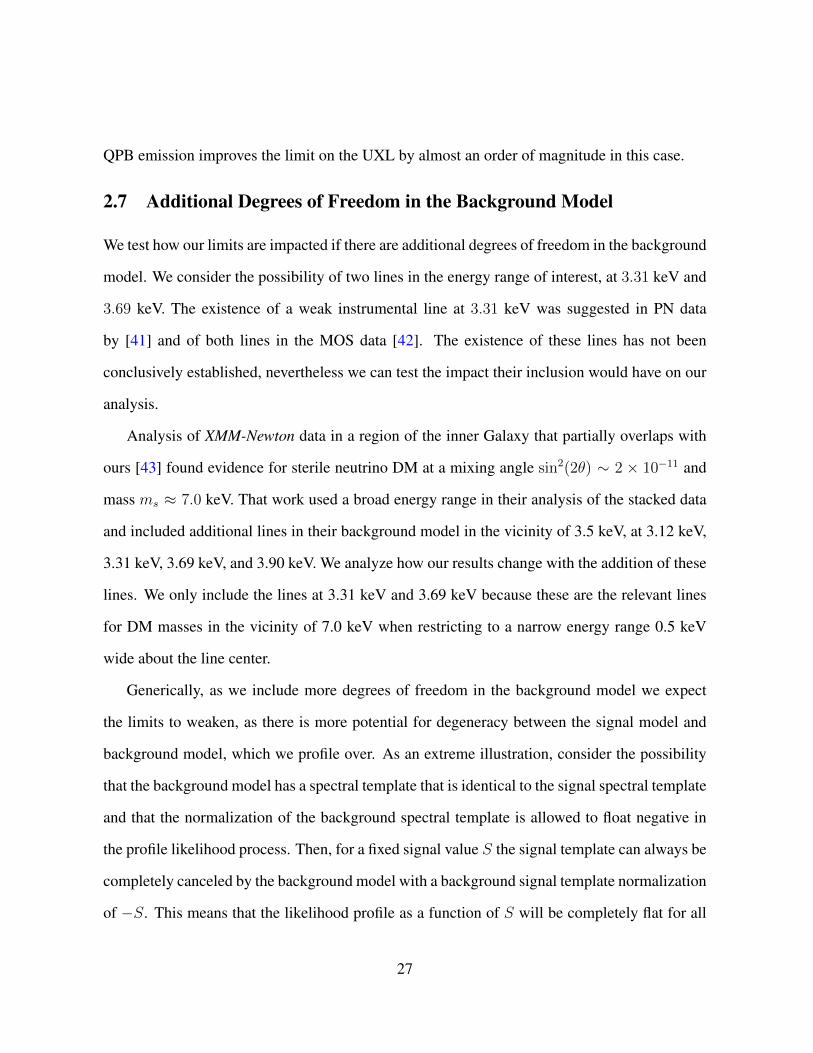
QPB emission improves the limit on the UXL by almost an order of magnitude in this case.

2.7 Additional Degrees of Freedom in the Background Model

We test how our limits are impacted if there are additional degrees of freedom in the background

model. We consider the possibility of two lines in the energy range of interest, at 3.31 keV and

3.69 keV. The existence of a weak instrumental line at 3.31 keV was suggested in PN data

by [41] and of both lines in the MOS data [42]. The existence of these lines has not been

conclusively established, nevertheless we can test the impact their inclusion would have on our

analysis.

Analysis of XMM-Newton data in a region of the inner Galaxy that partially overlaps with

ours [43] found evidence for sterile neutrino DM at a mixing angle sin2(2θ) ∼ 2 × 10−11 and

mass ms ≈ 7.0 keV. That work used a broad energy range in their analysis of the stacked data

and included additional lines in their background model in the vicinity of 3.5 keV, at 3.12 keV,

3.31 keV, 3.69 keV, and 3.90 keV. We analyze how our results change with the addition of these

lines. We only include the lines at 3.31 keV and 3.69 keV because these are the relevant lines

for DM masses in the vicinity of 7.0 keV when restricting to a narrow energy range 0.5 keV

wide about the line center.

Generically, as we include more degrees of freedom in the background model we expect

the limits to weaken, as there is more potential for degeneracy between the signal model and

background model, which we profile over. As an extreme illustration, consider the possibility

that the background model has a spectral template that is identical to the signal spectral template

and that the normalization of the background spectral template is allowed to float negative in

the profile likelihood process. Then, for a fixed signal value S the signal template can always be

completely canceled by the background model with a background signal template normalization

of −S. This means that the likelihood profile as a function of S will be completely flat for all

27

S. We can never find evidence for DM with this background model, but we will also set limits

that are arbitrarily weak, meaning that we will not rule out a real signal if one were present. The

background model we use with the addition of the two extra lines, whose normalizations are

allowed to go negative, does not have a complete degeneracy with the signal model, but there is

a partial degeneracy which leads to weaker limits as compared to the power-law model we use

in our fiducial analysis.

We illustrate the difference between the two background models with a simple example. We

generate Monte Carlo data using the best-fitting background model shown in Fig. S7 for the PN

camera of observation ID 0653550301, our most constraining exposure, as given in Table S1.

The Monte Carlo is generated under the null hypothesis, so there is no signal in the data. We

then analyze the simulated data for a signal at ms = 7.1 keV with our fiducial background

model and with the background model that has two extra lines at 3.31 keV and 3.69 keV. The

profile likelihoods for these different analyses are shown in Fig. S12A. The profile likelihood

with extra lines is broader than the fiducial profile likelihood. As a result, the limit obtained

with the background model containing extra lines is weaker by approximately a factor of two in

this case.

The degeneracy between the signal and background model in the profile likelihood is il-

lustrated in Fig. S13, where we show the best-fitting models for fixed signal fluxes with both

the fiducial background model and the background model including the extra lines. In the

presence of a signal, the analysis including the extra lines still recovers the injected signal

strength, but the significance of the detection is reduced because the background model is semi-

degenerate with the signal. Fig. S12B shows the profile likelihoods for analyses of the same

simulated datasets used in the example but now with the addition of a synthetic signal with

sin2(2θ) = 1.8 × 10−10. Both the fiducial analysis and the analysis including the extra lines

find the injected signal strength within 68% confidence, but the significance of the detection

28

−2 −1 0 1 2sin2(2θ) ×10−10

0

2

4

6

8

10

12

2δlo

gL

fiducial

extra lines

(A)

−1 0 1 2 3 4 5sin2(2θ) ×10−10

0

2

4

6

8

10

12

2δlo

gL

fiducial

extra lines

(B)

Figure S12: The effects of adding extra lines on the profile likelihood. (A) The profilelikelihood for a Monte Carlo-generated dataset with no DM decay signal. The solid black lineindicates the results using our fiducial analysis, while the dotted red line indicates the resultswhen including the lines at 3.31 keV and 3.69 keV. The analysis with extra lines sets weakerlimits on the sterile-active mixing angle, due to the partial degeneracy between the backgroundand signal models. (B) The profile likelihood for a Monte Carlo-generated dataset with aninjected signal of sin2(2θ) = 1.8× 10−10, indicated by the vertical dotted black line. Again, theanalysis with the extra lines sets weaker limits.

29

3.3 3.4 3.5 3.6 3.7 3.8E [keV]

75

100

125

150

cou

nts

sin2(2θ) = 1.8× 10−10

extra lines

fiducial

(A)

3.3 3.4 3.5 3.6 3.7 3.8E [keV]

75

100

125

150

cou

nts

sin2(2θ) = 3.6× 10−10

(B)

3.3 3.4 3.5 3.6 3.7 3.8E [keV]

75

100

125

150

cou

nts

sin2(2θ) = 5.4× 10−10

(C)

Figure S13: The effects of adding extra lines on the fitted model. The best-fitting modelsassuming a DM mass of 7.1 keV for fixed signal strengths (A, sin2(2θ) = 1.8 × 10−10; B,sin2(2θ) = 3.6 × 10−10; C, sin2(2θ) = 5.4 × 10−10) for the fiducial background model (redline) and the background model with extra lines (black line). The data shown (black points) isthe Monte Carlo data analyzed in the left side of Fig. S12.

30

is reduced for the analysis with extra lines, as may be seen from the likelihood profile being

broader in this case.

We perform this analysis across our ensemble of exposures and present the limits in Fig. S14A.

We show the limits for the MOS datasets, the PN datasets, and the combination of both datasets

(joint). We show the MOS and PN limits separately to account for the possibility that the extra

lines affect one detector but not the other. As expected, the limits are weaker when including

the extra lines in the background model. However, the limits (from both MOS and PN datasets

independently) remain inconsistent with the DM interpretation of the UXL and the best-fitting

parameters from the blank-sky analysis in [43]. In the vicinity of 7.0 keV we find no evidence

for DM, as in shown in Fig. S14B. For this analysis we restrict the exposure times of the individ-

ual exposures to be greater than 10 ks to ensure the model fitting of the individual exposures is

well converged. This reduces the total exposure time to∼27.2 Ms, which does not substantially

affect the projected sensitivity.

We investigate whether the model fitting favors the background model with the two extra

lines over the fiducial model. Adding two extra degrees of freedom to the background model

should lead to an improved fit to the data. If the data is well described by the fiducial background

model then we might expect that using the model with extra lines, which has two extra degrees

of freedom, would cause a decrease in the χ2 for the best-fitting background model that follows

a χ2-distribution with two degrees of freedom. This is what we observe, as is shown in Fig. S15

for the particular case of mχ = 7.1 keV. We show the average χ2 difference, over all of the

exposures included in the analysis, between the fiducial background model and the model with

two extra lines, for the MOS and PN datasets independently and combined. The distributions

follow the appropriate χ2-distributions with two degrees of freedom.

31

6.8 6.9 7.0 7.1 7.2 7.3ms [keV]

10−12

10−11

10−10

10−9

sin

2 (2θ)

1

2

3 4

5

6

7

8

9

10

fiducial limit

extra lines (joint)

extra lines (MOS)

extra lines (PN)

(A)

6.8 6.9 7.0 7.1 7.2 7.3

ms [keV]

0

1

2

3

4

5

TS

fiducial

extra lines (joint)

extra lines (MOS)

extra lines (PN)

(B)

Figure S14: The effects of adding extra lines on the limits and TS. (A) The one-sided power-constrained 95% limits on sin2(2θ) as a function of the DM mass ms with the analysis withextra lines, compared to the fiducial limit and the parameter space from Fig. 2. We show theextra-line limits for the MOS and PN datasets independently and combined. The fiducial limitis stronger than the limit when including the extra lines. Nevertheless, the latter limit remainsinconsistent with the detections shown in Fig. 2, and the best-fitting parameters in [43] (redpoint). Our conclusions are not dependent on our choice of background model. (B) The teststatistic (TS) in favor of a decaying DM interpretation of the UXL as a function of the DM massms with the analysis with extra lines (black), compared to the fiducial TS (red). The green andyellow regions indicate 1σ and 2σ detections, respectively. No evidence for decaying DM ineither analysis is found.

32

2.8 Analysis of Disjoint Regions

We performed our analysis separately in multiple disjoint regions. We determine the TS in fa-

vor of DM within each region, and investigate whether it is consistent with the null hypothesis.

Fig. 3B shows the distribution of TSs for the individual exposures combined into the joint like-

lihood used in our fiducial analysis. However, in the presence of a small signal of strength near

our limiting value, this distribution may resemble the null hypothesis χ2 distribution, because

the effect on each individual exposure is small. Here we extend this check, by determining the

TS distribution in different regions.

Our fiducial analysis includes exposures within 5 and 45 of the Galactic Center. We now

consider dividing the region between 5 and ∼90 into four approximately equal exposure re-

gions, with the first region being our fiducial region, the second region extending from 45 to

62.2, the third region from 62.2 to 74.0, and the fourth from 74.0 to 83.4. All of these

regions have approximately 30.6 Ms of exposure, by construction. These regions would also be

approximately equal area, though in practice we see that the area of the concentric circular re-

gions decreases with distance from the Galactic Center. This is due to our flux cut on individual

exposures, which is less frequently satisfied for observations closer to the Galactic Center. We

compute the TS for analyses in each of these regions for three different mass points: ms = 6.9,

7.1, and 7.3 keV. We use the three independent mass points to improve the statistics when con-

structing the TS distribution. We then combine the TSs from the different mass points; the

resulting distribution of TSs is shown in Fig. S16. The distribution TSs follows the one-sided

χ2 distribution, as expected under the null hypothesis, though the number of independent anal-

yses Nanal is limited. This disfavors the presence of large systematic uncertainties, indicating

that our uncertainty is is dominated by statistical variations. The bin with TS = 0 is not shown

in Fig. S16; instead, we state it here. We expect that half of our 12 analyses should produce

TS = 0 and find 7+3.8−2.6, consistent with the predicted number of 6.

33

In Fig. S16B, we show how, atms = 7.1 keV, our best-fitting mixing angle sin2(2θ) changes

between the analyses in the four independent regions. We show the expectations under the null

hypothesis; for statistical consistency, we must include the possibility of negative sin2(2θ). If

our background model systematically under predicts the counts at energies ∼ms/2, but also a

real signal is present, the evidence for that real signal could be obscured. However, in that case

regions further from the Galactic Center would have a smaller signal contribution, so we would

expect the best-fit mixing angle to become more and more negative. This is not what we see

(there is a slight trend in the other direction). This indicates that our analysis is statistically

limited and that there is not a systematic effect at ms/2 obscuring the presence of a signal.

By choosing regions with similar exposure times as our fiducial analysis, the number of

regions considered above Nanal is limited. We can seek to find an intermediary regime between

this result and Fig. 3B by decreasing the size of our concentric regions. This, however, comes at

the cost of reduced sensitivity, because each individual analysis does not have as much exposure.

In the extreme limit of individual exposures, the limits obtained are shown in Fig. S6. As an

illustration, we consider taking 45 approximately equal-exposure regions, with the first region

extending from 5 to 10, the second from 10 to 15.4, and the last from 88.6 to 88.9. All

of the sub-regions have approximately 3 Ms of exposure. The distribution of TSs at ms = 6.9

keV, 7.1 keV, and 7.3 keV over these analyses is shown in the right panel of Fig. S17B. The TS

distribution is consistent with the expectation under the null hypothesis. This again indicates

that the dominant source of uncertainty is statistical and not systematic. The limits obtained

from the inner four rings are shown in Fig. S17A. While these limits are slightly weaker than in

our fiducial analysis, they are each inconsistent with the decaying DM interpretation of the 3.5

keV line.

34

2.9 Analysis of Stacked Data

Our fiducial data analysis is based on the joint likelihood that combines the profile likelihoods

from the disjoint analyses of the individual exposures. An alternative analysis, as described in

the main text, is to instead stack the data from the individual exposures and then analyze the

stacked data. The limits obtained from this procedure are consistent with those obtained from

our fiducial data analysis and, in particular, are in tension with the DM interpretation of the

UXL. In this section we provide additional details behind this analysis.

The stacked MOS and PN datasets are shown in Fig. 2 (see also Figs. S18A and B) from

3.3 keV to 3.8 keV. These datasets are constructed by summing the individual spectra. We then

fit models to these stacked spectra that consist of a null hypothesis component to describe the

smooth background emission and a signal component to model the contribution from a putative

UXL at e.g. 3.55 keV. We independently fit models to the MOS and PN data, since these

instruments have different instrument responses, in order to construct profile likelihoods for the

UXL flux as determined by the two cameras. We then join these two profile likelihoods together

in order to obtain our final constraint on the 3.55 keV UXL. Note that since all of the energy

bins shown in Fig. 2, for both the MOS and PN data, have over 103 counts, we use a Gaussian

likelihood instead of a Poisson likelihood.

The red curves in Fig. 2 are the best sums of the best-fit null hypothesis models from the

analyses of the individual exposures. While each of the curves that goes into the sum is modeled

as a combination of two power-law components, the combined spectrum does not need to follow

a simple power-law. However, as shown below, we find that a quadratic background model

with three model parameters is able to describe the data at the level of statistical noise. In

particular, we take the background model for the stacked data analysis to be dN/dE(E, θnuis) =

A + B (E/1 keV) + C (E/1 keV)2, where dN/dE are the fluxes appearing in Fig. 2 in units

of counts s−1keV−1, and where θnuis = A,B,C are the nuisance parameters. The signal

35

component is as shown in Fig. 2 and is obtained by forward modeling the 3.55 keV UXL

through the detector responses from each individual exposure and then summing the resulting

spectra. As seen in Fig. 2, the effect of the UXL is to produce a spectral feature with a width

∼200 eV, though that feature is narrower for the MOS data than for the PN data.

Fitting the quadratic background plus signal model to the PN (MOS) data produces a fit

with a χ2/DOF, for 50 − 4 DOF, of 1.14 (0.81). The expected 68% containment interval for

the χ2/DOF with 46 DOF under the null hypothesis is ∼[0.79, 1.21]; this interval contains the

values measured for both the PN and MOS data. We then compute the profile likelihood for

the signal-model flux parameter sin2(2θ) by profiling over the background nuisance parameters.

The profile likelihood is shown in Fig. S18C. We show the profile likelihoods for the PN and

MOS data analyzed separately and also for the combination. The 95% upper limit is found by

taking the upper value for sin2(2θ) under the condition 2∆ logL ≈ 2.71; this leads to the upper

limit sin2(2θ) < 5 × 10−12, which strongly constrains the DM interpretation of the 3.5 keV

UXL.

36

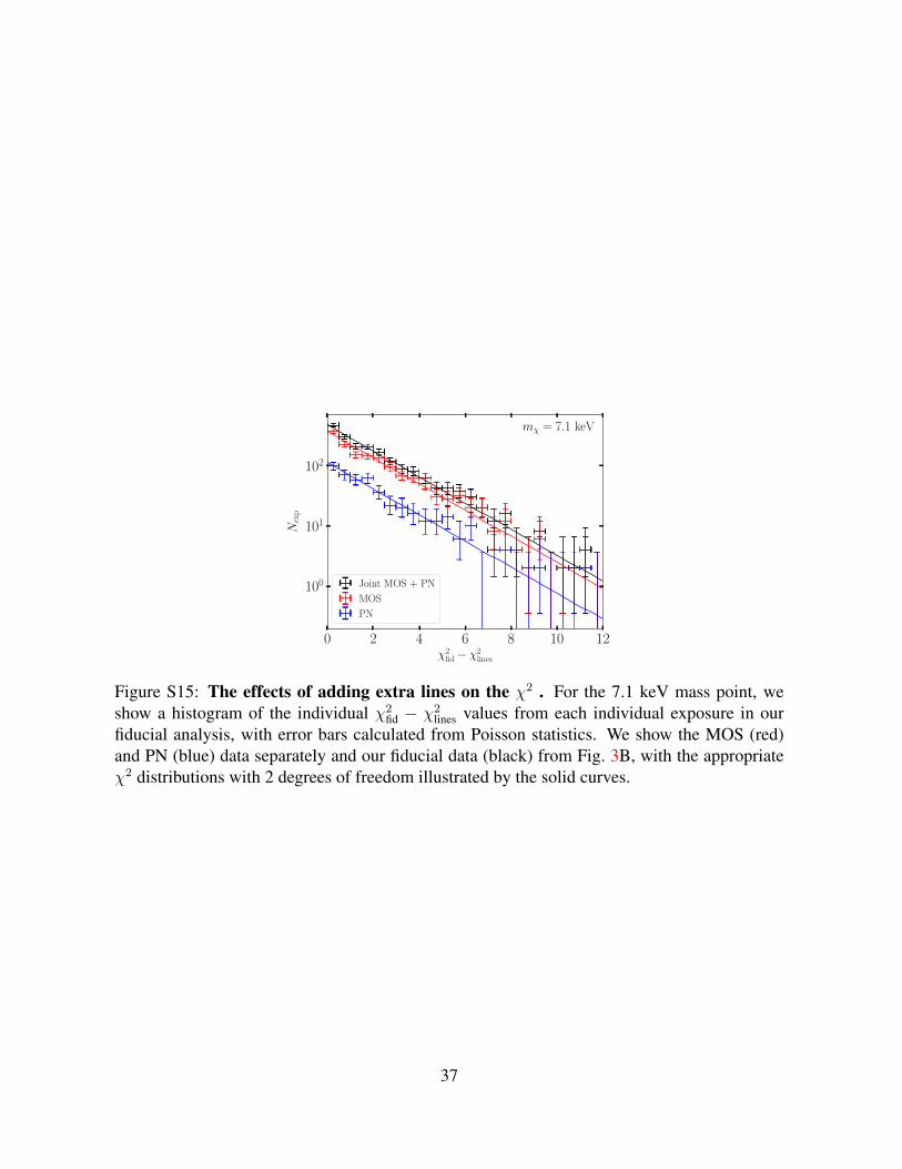
0 2 4 6 8 10 12χ2

fid − χ2lines

100

101

102

Nex

p

mχ = 7.1 keV

Joint MOS + PN

MOS

PN

Figure S15: The effects of adding extra lines on the χ2 . For the 7.1 keV mass point, weshow a histogram of the individual χ2

fid − χ2lines values from each individual exposure in our

fiducial analysis, with error bars calculated from Poisson statistics. We show the MOS (red)and PN (blue) data separately and our fiducial data (black) from Fig. 3B, with the appropriateχ2 distributions with 2 degrees of freedom illustrated by the solid curves.

37

0 2 4 6TS

10−1

100

101

dN

anal/d

(TS

)

(A)

0 20 40 60 80rmin [deg]

−10

−5

0

5

10

sin

2 (2θ)×

1012

best fit

1σ/2σ containment

(B)

Figure S16: Dividing the analysis into 4 concentric regions around the Galactic Center.(A) Distribution of TS values obtained from four independent regions, with three mass pointsconsidered for each, are shown in black, with error bars from Poisson statistics. The differentregions are our fiducial region used in the main text, as well as observations with 45 < r <62.2, 62.2 < r < 74.0, and 74.0 < r < 83.4, where r is the angle from the GalacticCenter. These regions have approximately 30.6 Ms of exposure each, with our fiducial set offlux and QPB cuts. We also show in red the expectation from statistical fluctuations of the nullhypothesis, as determined by the χ2 distribution. Note the bin with TS = 0 is excluded from thefigure, but the values are stated in the text. (B) The best fitting values (black circles) of sin2(2θ)for each of our four regions, identified by their minimum angle from the Galactic Center, forms = 7.1 keV. The green and yellow regions indicate 1σ and 2σ containment for these values,respectively.

38

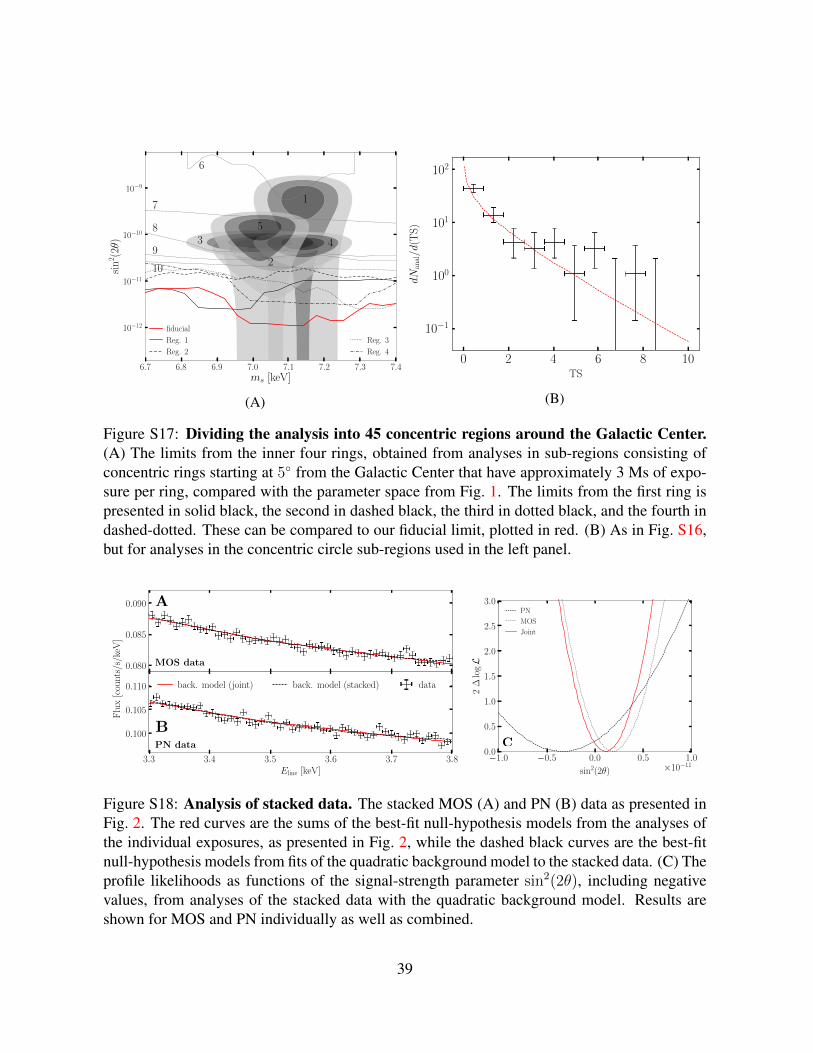
6.7 6.8 6.9 7.0 7.1 7.2 7.3 7.4ms [keV]

10−12

10−11

10−10

10−9

sin

2 (2θ)

1

2

3 4

5

6

7

8

9

10

Reg. 3

Reg. 4

fiducial

Reg. 1

Reg. 2

(A)

0 2 4 6 8 10TS

10−1

100

101

102

dN

anal/d

(TS

)

(B)

Figure S17: Dividing the analysis into 45 concentric regions around the Galactic Center.(A) The limits from the inner four rings, obtained from analyses in sub-regions consisting ofconcentric rings starting at 5 from the Galactic Center that have approximately 3 Ms of expo-sure per ring, compared with the parameter space from Fig. 1. The limits from the first ring ispresented in solid black, the second in dashed black, the third in dotted black, and the fourth indashed-dotted. These can be compared to our fiducial limit, plotted in red. (B) As in Fig. S16,but for analyses in the concentric circle sub-regions used in the left panel.

0.080

0.085

0.090

Flu

x[c

ount

s/s/

keV

]

MOS data

3.3 3.4 3.5 3.6 3.7 3.8Eline [keV]

0.100

0.105

0.110

count

s/s/

keV

PN data

back. model (joint) back. model (stacked) data

A<latexit sha1_base64="A4SUZflqmyigAm3/uoNMENOCPkY=">AAAB8XicbVDLSgMxFL1TX7W+qi7dhBbBVZnxgS4rblxWsA9sS8mkmTY0kxmSO0IZ+hduXCji1r9x59+YaWeh1QOBwzn3knOPH0th0HW/nMLK6tr6RnGztLW9s7tX3j9omSjRjDdZJCPd8anhUijeRIGSd2LNaehL3vYnN5nffuTaiEjd4zTm/ZCOlAgEo2ilh15IcewH6fVsUK66NXcO8pd4OalCjsag/NkbRiwJuUImqTFdz42xn1KNgkk+K/USw2PKJnTEu5YqGnLTT+eJZ+TYKkMSRNo+hWSu/txIaWjMNPTtZJbQLHuZ+J/XTTC46qdCxQlyxRYfBYkkGJHsfDIUmjOUU0so08JmJWxMNWVoSyrZErzlk/+S1mnNO6td3J1X65W8jiIcQQVOwINLqMMtNKAJDBQ8wQu8OsZ5dt6c98Vowcl3DuEXnI9vokqQzA==</latexit>

B<latexit sha1_base64="UVCrK1d1G8rT1OH2knfr04bNaRU=">AAAB8XicbVDLSgMxFL1TX7W+qi7dhBbBVZnxgS6LblxWsA9sS8mkmTY0kxmSO0IZ+hduXCji1r9x59+YaWeh1QOBwzn3knOPH0th0HW/nMLK6tr6RnGztLW9s7tX3j9omSjRjDdZJCPd8anhUijeRIGSd2LNaehL3vYnN5nffuTaiEjd4zTm/ZCOlAgEo2ilh15IcewH6fVsUK66NXcO8pd4OalCjsag/NkbRiwJuUImqTFdz42xn1KNgkk+K/USw2PKJnTEu5YqGnLTT+eJZ+TYKkMSRNo+hWSu/txIaWjMNPTtZJbQLHuZ+J/XTTC46qdCxQlyxRYfBYkkGJHsfDIUmjOUU0so08JmJWxMNWVoSyrZErzlk/+S1mnNO6td3J1X65W8jiIcQQVOwINLqMMtNKAJDBQ8wQu8OsZ5dt6c98Vowcl3DuEXnI9vo8+QzQ==</latexit>

1.0 0.5 0.0 0.5 1.0

sin2(2) 1011

0.0

0.5

1.0

1.5

2.0

2.5

3.0

2

logL

PN

MOS

Joint

C<latexit sha1_base64="orAJ4evLKSkAv2DIgCMM2oIBWNo=">AAAB8XicbVDLSgMxFL1TX7W+qi7dBIvgqsz4QJfFblxWsA9sS8mkd9rQTGZIMkIZ+hduXCji1r9x59+YaWeh1QOBwzn3knOPHwuujet+OYWV1bX1jeJmaWt7Z3evvH/Q0lGiGDZZJCLV8alGwSU2DTcCO7FCGvoC2/6knvntR1SaR/LeTGPsh3QkecAZNVZ66IXUjP0grc8G5Ypbdecgf4mXkwrkaAzKn71hxJIQpWGCat313Nj0U6oMZwJnpV6iMaZsQkfYtVTSEHU/nSeekROrDEkQKfukIXP150ZKQ62noW8ns4R62cvE/7xuYoLrfsplnBiUbPFRkAhiIpKdT4ZcITNiagllitushI2poszYkkq2BG/55L+kdVb1zquXdxeV2k1eRxGO4BhOwYMrqMEtNKAJDCQ8wQu8Otp5dt6c98Vowcl3DuEXnI9vrvSQ7g==</latexit>

Figure S18: Analysis of stacked data. The stacked MOS (A) and PN (B) data as presented inFig. 2. The red curves are the sums of the best-fit null-hypothesis models from the analyses ofthe individual exposures, as presented in Fig. 2, while the dashed black curves are the best-fitnull-hypothesis models from fits of the quadratic background model to the stacked data. (C) Theprofile likelihoods as functions of the signal-strength parameter sin2(2θ), including negativevalues, from analyses of the stacked data with the quadratic background model. Results areshown for MOS and PN individually as well as combined.

39