The Cost-Effectiveness of Midwifery Staffing and Skill Mix on Maternity Outcomes

A Report for The National Institute for Health and Care Excellence

Professor Graham Cookson, Professor Simon Jones, Mr Jeremy van Vlymen & Dr Ioannis Laliotis

University of Surrey

Final Report: December 2014

ii

iii

University of Surrey

One of the UK’s leading professional, scientific and technological universities in the UK, the

University of Surrey ranked 39th in the prestigious Top 100 List of the world’s most international

universities, part of the Times Higher Education (THE) World University rankings for 2013-

14. Actively involved in successive research collaborations with industrial and research partners

across Europe since the Fourth Framework Programme, the University of Surrey received funding for

160 projects in the Seventh Framework Programme, including 26 Marie Curie fellowships.

Department of Health Care Management & Policy

The Department of Health Care Management and Policy (DHCMP) at the University of Surrey has

been involved in quality improvement interventions over the last 15 years, primarily for long term

conditions in the UK and internationally. Our interests are how to measure quality and health

outcomes from routine data, quality improvement and technology trials, and integrating the use of

the computer into the clinical consultation.

Despite being a small group, we have over 150 full length peer review scientific research

publications; in addition to over 100 other peer review journal articles, letters or editorials and in

excess of this number of conference abstracts. We have direct links with an excellent group of

international collaborators; and links through the primary care informatics working groups of IMIA

and EFMI (the International and European informatics organisations).

The Economics group in DHCMP has 10 members and is led by Professor Graham Cookson. The

principal focus of the group is on the determinants of health care provider’s productivity, the

efficiency and effectiveness trade-off in health care, and the role of the health care workforce in this

relationship.

iv

Acknowledgements

In November 2013, National Institute for Health and Care Excellence (NICE) was asked by the

Department of Health (DH) and NHS England to develop new guideline outputs which focus on safe

staffing. In June 2014, NICE commissioned Professor Graham Cookson and his team at the University

of Surrey to produce an economic evaluation of the effects of midwifery staffing and skill mix on

outcomes of care in maternity settings. This report is the result of that work. GC took overall

responsibility for the project, produced the report and conducted the economic evaluation. JvV

performed the statistical analysis with assistance from SJ and IL performed the econometric analysis,

both contributed to writing the report. SJ was responsible for internal quality assurance. Rachel

Byford and David Burleigh were responsible for data management and production, and for

information governance. The authors would like to thank: the team at NICE but in particular Jasdeep

Hayre and Lorraine Taylor; Dr Chris Bojke (University of York); Professor John Appleby (The King’s

Fund) and the members of the NICE Safe Staffing Advisory Committee for helpful comments and

insights into the production of this report.

Any errors or omissions remain our own.

Disclaimer and Declaration of Interests

Professor Cookson was a co-investigator of an NIHR funded study1 of staffing and outcomes in

maternity services, and was a co-author of the final project report (Sandall et al., 2014) which is

referred to in this report as well as in both the Bazian (2014) and Hayre (2014) evidence reviews

used by the SSAC. Additionally, he was also one of Vania Gerova’s Ph.D. supervisors whose research

has been reviewed in Bazian (2014). GC performed the economic evaluation for the acute nursing

NICE Safe Staffing Guideline. He currently receives funding from The Leverhulme Trust2 which is

partially supporting research on the healthcare workforce including maternity services. IL also works

on this project. JvV and SJ have nothing to declare.

1 NIHR study HS&DR - 10/1011/94: The efficient use of the maternity workforce and the implications for safety

& quality in maternity care: An economic perspective, March 2012-October 2014. Further details are available from: http://www.nets.nihr.ac.uk/projects/hsdr/10101194. The final report can be accessed at: http://www.journalslibrary.nihr.ac.uk/hsdr/volume-2/issue-38#hometab4 2 Further details can be found at http://www.deliveringbetter.com

v

Table of Contents

1 Executive Summary .................................................................................................. 10

2 Introduction ............................................................................................................. 11

2.1 The Role of Economic Evaluation in the NICE process ..................................................... 11

2.2 Safe Staffing.................................................................................................................. 13

2.3 Purpose of this report ................................................................................................... 15

2.4 Structure of this report .................................................................................................. 15

3 Methods ................................................................................................................... 16

3.1 Economic Model Scope ................................................................................................. 16

3.2 CEA Methodology ......................................................................................................... 17

3.1 Costs............................................................................................................................. 18

3.2 Evidence of cost-effectiveness of interventions .............................................................. 19

3.3 Effectiveness of Staffing on Outcomes ........................................................................... 21

3.3.1 Data and Variables ........................................................................................................... 22

3.3.2 Statistical Methodology.................................................................................................... 31

3.3.3 Econometric Methodology ............................................................................................... 33

4 Results ..................................................................................................................... 37

4.1 Statistical Analysis ........................................................................................................ 37

4.1.1 Descriptive Analysis .......................................................................................................... 37

4.1.2 Statistical (Regression) Results ......................................................................................... 52

4.2 Econometric Analysis .................................................................................................... 60

4.3 Cost-Effectiveness Analysis ............................................................................................ 65

4.3.1 Economic Model Parameters ........................................................................................... 65

4.3.2 Cost-Effectiveness ............................................................................................................ 69

4.3.3 Sensitivity Analysis ........................................................................................................... 69

5 Discussion ................................................................................................................ 72

5.1 Statistical Analysis Limitations ....................................................................................... 72

5.2 Cost-Effectiveness Analysis limitations .......................................................................... 74

5.3 Recommendations for Future Research ......................................................................... 74

5.4 Evidence Summary ........................................................................................................ 75

6 References ............................................................................................................... 78

vi

7 Appendix A: Full Statistical Results ........................................................................... 80

vii

List of Figures

Figure 1: Incremental Cost-Effectiveness Ratio .................................................................................... 12

Figure 2: FTE Registered Midwives per 100 Maternities 2003-2013 .................................................... 47

Figure 3: FTE Doctors per 100 maternities 2003-2013 ......................................................................... 47

Figure 4: FTE Support Workers per 100 maternities 2003-2013 .......................................................... 48

Figure 5: Total Staff per 100 Maternities 2003-2013 ........................................................................... 48

Figure 6: Doctors to Midwives Ratio 2003-2013 .................................................................................. 49

Figure 7: Support Workers to Midwives Ratio 2003-2013 ................................................................... 49

Figure 8: Managers to All Staff Ratio 2003-2013 .................................................................................. 50

Figure 9: Hospital Load Ratio Variation 2013 ....................................................................................... 52

viii

List of Tables

Table 1 Economic Model Parameters and Sources............................................................................... 18

Table 2: NHS Employment Costs – Source: PSSRU 2013. ..................................................................... 18

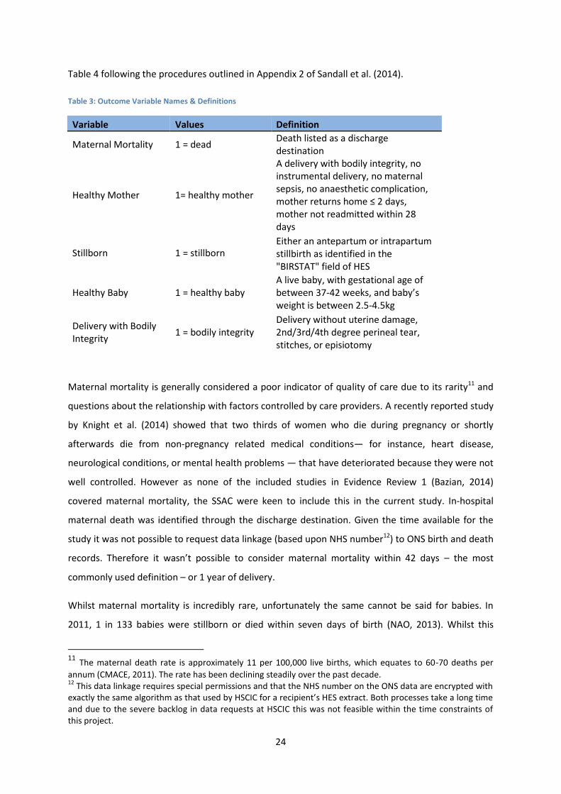
Table 3: Outcome Variable Names & Definitions ................................................................................. 24

Table 4: Explanatory Variables Labels & Definitions ............................................................................ 30

Table 5: Descriptive Statistics of Outcomes .......................................................................................... 37

Table 6: Descriptive Statistics – Hospital Episode Statistics Data ......................................................... 40

Table 7: Staffing Data Descriptive Statistics – FTE per 100 deliveries .................................................. 46

Table 8: Simplified Statistical Findings .................................................................................................. 56

Table 9: Baseline parameter results for a generalized linear production function (Ordinary Least

Squares estimates). The total number of deliveries is used as the output measure ................... 61

Table 10 Estimates of marginal productivities and Hicks elasticities of complementarity .................. 63

Table 11: Baseline parameter results for a generalized linear production function (Fixed Effects

estimates). The total number of deliveries is used as the output measure ................................. 64

Table 12: Estimates of marginal productivities and Hicks elasticities of complementarity ................. 65

Table 13: Sensitivity Modelling Parameters ......................................................................................... 68

Table 14: ICER for Maternal Outcomes................................................................................................. 68

Table 15: Sensitivity Analysis Results .................................................................................................... 71

Table 16: Healthy Mother Full Regression Results ............................................................................... 80

Table 17: Maternal Mortality Full Results ............................................................................................. 83

Table 18: Bodily Integrity Full Regression Results ................................................................................ 86

Table 19: Stillborn Full Regression Results ........................................................................................... 89

Table 20: Full Results Healthy Baby Regression .................................................................................... 92

Table 21: Healthy Baby Full Regression Results .................................................................................... 94

ix

10

1 Executive Summary

In November 2013, National Institute for Health and Care Excellence (NICE) was asked by the

Department of Health (DH) and NHS England to develop new guideline outputs which focus on safe

staffing. In July 2014, NICE commissioned this report which aims to estimate the cost-effectiveness

of altering midwifery staffing and skill mix on outcomes of care in hospital maternity wards.

Following a systematic Evidence Review (Bazian, 2014), the Safe Staffing Advisory Committee (SSAC)

set the scope of this report to consider five outcomes: maternal and infant mortality, healthy

mother and baby and bodily integrity.

There is limited evidence on the association between midwifery staffing levels, skill mix and clinical

outcomes in the UK, and the two studies that provide any economic insights are severely limited.

The evidence suggests that increased midwife staffing may be associated with an increased

likelihood of delivery with bodily integrity (no uterine damage, 2nd/3rd/4th degree tear, stitches,

episiotomy, or Caesarean-section), reduced maternal readmissions within 28 days, and reduced

decision-to-delivery times for emergency Caesarean-sections. A number of issues were identified

with the extant literature including potential endogeneity. As a result, new statistical analysis was

commissioned to produce effectiveness measures for the economic evaluation. This research

analysed delivery records from Hospital Episode Statistics from 2003-2013 linked to staffing data

from the Workforce Census.

At present, this is the largest and most robust study of maternal outcomes using administrative data.

The study found that midwifery staffing levels (FTE midwife per 100 deliveries) was positively and

statistically significantly associated with healthy mother and delivery with bodily integrity rates,

although the relationships were weak. Most of the variation in outcomes occurred at the individual,

patient level rather than at trust level, with clinical risk having the largest effect.

The trust-level intervention considered was an increase in 1 FTE midwife per 100 deliveries. The

effectiveness of the intervention was taken from the new statistical analysis. It was not possible to

combine the benefits of the intervention into a common metric (e.g. QALYs) therefore it is

impossible to ascertain the overall cost-effectiveness of changing midwife staffing or skill mix.

Instead a Cost-Effectiveness Analysis was performed and Incremental Cost Effectiveness Ratios

(ICERs) were computed separately for each maternity service outcome which was shown to have an

association with staffing during the statistical analysis.

The reported ICERs were £85,560 per additional “healthy mother” and £193,426 per mother with

“bodily integrity”. No other outcomes were found to be associated with midwifery staffing levels.

11

However, despite the findings being based upon the best available evidence, caution should be

exercised when using these results as there is great uncertainty as to the benefits of staffing

interventions due to potential endogeneity and as a result of aggregate staffing measures. Further

research and primary data collection may be required to resolve these issues.

2 Introduction

2.1 The Role of Economic Evaluation in the NICE process

The NHS has limited resources and almost endless uses of those resources. Therefore, when a new

intervention or technology is adopted some amount of the existing health care provision will be

displaced. This is what economists refer to as the ‘opportunity cost’ of an intervention. To maximise

society’s health gain from the NHS’s limited budget, and to make decisions on whether to adopt new

interventions in a coherent and transparent manner an economic evaluation is performed.

NICE plays a central role in the process by advising the NHS on the (clinical) effectiveness and cost-

effectiveness of health care interventions and technologies. An intervention is cost-effective if it

generates more health gain than it displaces as a result of the additional costs imposed on the

system. Sometimes a new intervention dominates the existing best practice by being both cheaper

and more effective, in which case the outcome is clear. More often the proposed intervention is

more expensive and may be more effective.

An economic analysis is usually required because the costs and/or benefits of a new intervention are

uncertain. There are numerous reasons for this uncertainty. For example, there may be several

small-scale studies reporting conflicting levels of effectiveness of a new treatment, or the context or

population of these studies may not be wholly representative of the NHS patient population.

Alternatively, widespread adoption of a new intervention may alter the market and therefore the

price of the intervention. Frequently, the costs of an intervention are borne today but the benefits

occur over several years into the future. All of these situations require careful modelling to enable a

fair comparison of alternative outcomes. Inevitably, the economist must make assumptions about

the most plausible values of the costs and benefits of an intervention based upon the best available

evidence.

To illustrate the impact of these assumptions on the results of the economic analysis a sensitivity

analysis is performed. This technique varies the main assumptions used to produce the base case to

include plausible but extreme values of these assumptions. If varying these assumptions has little

12

effect on the result of the economic analysis then we can be confident that the findings are robust

and representative of the truth. If the results of the economic analysis vary considerably during the

sensitivity analysis then additional research or evidence may be required to establish the truth, and

less weight should be given to the economic evaluation in any decision making process.

NICE prefers that cost-effectiveness is reported as a cost per quality-adjusted life year (QALY)

because this enables comparisons across different disease areas, populations or even between

service level and disease-specific treatments to be made on a common metric. Additionally, it has

the benefit of combining the multiple benefits of an intervention into a single outcome measure.

QALYs are measured by estimating the health utility or value of being in different health states

(where 1 is equivalent to a notional health state of perfect health and 0 is being dead) and are

combined with the length of time spent in each of these health states as a result of the intervention.

When it is not possible to measure QALYs, it is appropriate to report the benefits of the intervention

in terms of some disease or topic specific outcome. For example, in terms of increasing ward level

staffing the outcome may be the number of falls prevented.

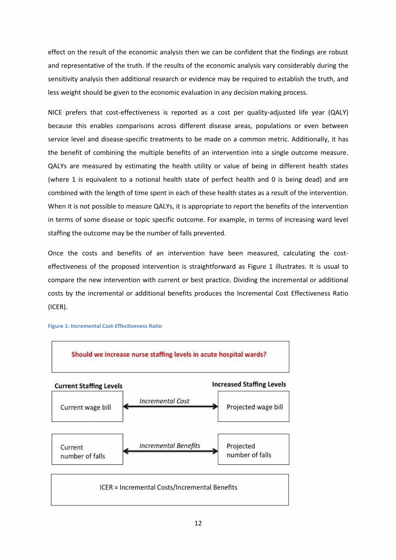
Once the costs and benefits of an intervention have been measured, calculating the cost-

effectiveness of the proposed intervention is straightforward as Figure 1 illustrates. It is usual to

compare the new intervention with current or best practice. Dividing the incremental or additional

costs by the incremental or additional benefits produces the Incremental Cost Effectiveness Ratio

(ICER).

Figure 1: Incremental Cost-Effectiveness Ratio

13

As a concrete example, consider a hypothetical situation where the increase in staffing intervention

was to add one additional nurse per ward at a cost of £31,8673 per annum and in one year the only

effect was to reduce the number of falls by 4. The ICER in this example would be £7,967 per averted

fall.

If the new intervention is less effective and more costly than existing practice it is not cost-effective,

and if it is more effective and cheaper than existing practice it is cost-effective. In these

circumstances the outcome is straightforward. Usually however, the new intervention is either less

effective but significantly cheaper, or more effective but also more expensive. In these

circumstances the ICER is compared to the value of the interventions or treatments which are

displaced if the new intervention is adopted: the opportunity cost. This is usually thought to be in

the region of £20,000-£30,000 per QALY. There is little guidance available when the ICER is

expressed in the original units of effects (e.g. falls prevented) and careful consideration needs to be

given as to the value-for-money represented by the intervention in these situations.

2.2 Safe Staffing

Ensuring that staffing levels are sufficient to maximise patient safety and quality of care, whilst

optimising the allocation of financial resources, is an important challenge for the NHS. The National

Institute for Health and Care Excellence (NICE) has been asked by the Department of Health and NHS

England to develop an evidence-based guideline on safe and cost-effective midwifery staffing levels

in NHS trusts.

A systematic literature review concluded that the amount of evidence on the relationship between

midwifery staffing and outcomes is limited (Bazian, 2014). Their review included 8 studies with most

of them using cross-sectional designs, which severely limited their ability to detect potential

causality. However, all of the included studies were carried out in the UK and are therefore expected

to be applicable to the UK.

Overall few significant associations between midwife staffing levels and outcomes were identified.

The evidence suggests that increased midwife staffing may be associated with an increased

3 This figure calculated by adding the mean annual basic salary (excluding overtime) of an Agenda for Change

Band 5 nurse of £25,744 to the mean on-costs of employing the nurse of £6,123 taken from the Personal Social Services Research Unit costings for July 2013-June 2013. It excludes overheads, capital costs, overtime, London weightings or training and qualification costs.

14

likelihood of delivery with bodily integrity4, reduced maternal readmissions within 28 days, and

reduced decision-to-delivery times for emergency Caesarean-sections. However, it may not be

associated with overall Caesarean-section rates, composite ‘healthy mother5’ or ‘health baby6’

outcomes, rates of ‘normal’ or ‘straightforward’ births, or stillbirth or neonatal mortality.

Interpretation is also complicated by the use of differing, but overlapping, outcomes in different

studies. For example, although delivery with bodily integrity was increased in one study, another

study suggested a possible reduction in straightforward birth with increasing levels of midwife

staffing, and straightforward birth includes some of the same outcomes (no intrapartum Caesarean-

section or 3rd/4th degree perineal trauma, as well as no birth without forceps or ventouse or blood

transfusion).

Only one study formally assessed the interaction between modifying factors (maternal clinical risk

and parity) and midwife staffing levels, therefore limited conclusions can be drawn about their

effects. No studies were identified which assessed the links between midwife staffing and on

maternal mortality or never events (such as maternal death due to post-partum haemorrhage after

elective caesarean section, wrongly prepared high-risk injectable medication, intravenous

administration of epidural medication, or retained foreign objects post-procedure) or serious

fetal/neonatal events such as Erb’s palsy secondary to shoulder dystocia, meconium aspiration

syndrome, hypoxic ischaemic encephalopathy (HIE). The SSAC requested that maternal mortality be

added to the analysis as none of the included studies in Evidence Review 1 included this outcome

(Bazian, 2014).

Limited evidence was identified on potential modifiers of the effect of midwife staffing levels on

outcomes, therefore limited conclusions can be drawn about their effects. Only one study (Sandall et

al. 2014) formally assessed potential interactions between modifying factors and midwife staffing

levels. Its findings suggested that, maternal clinical risk and parity both appear to be modifiers, and

to themselves have a large impact on outcomes. This is a serious weakness of the other evidence

because it is probable that clinical risk is associated with staffing decisions. Excluding a measure of

clinical risk from models may invalidate the findings due to omitted variable bias, which leads to an

overestimation of the effect of staffing levels on outcomes.

4 A delivery with bodily integrity is defined as one without uterine damage, 2nd/3rd/4th degree tear, stitches,

episiotomy, or Caesarean-section. 5 A ‘healthy mother’ is defined as a mother who has a delivery with bodily integrity, no instrumental delivery,

no maternal sepsis, no anaesthetic complication, mother returns home ≤ 2 days, mother not readmitted within 28 days 6 A ‘healthy baby’ is defined as a live baby, with gestational age of between 37-42 weeks, and baby’s weight is

between 2.5-4.5kg

15

2.3 Purpose of this report

This report aims to assess the cost-effectiveness of altering midwifery staffing levels and skill mix in

the English NHS. It accompanies the Evidence Review produced by the Bazian (2014) and Hayre

(2014).

2.4 Structure of this report

The next section details the methodologies and data used for both the economic evaluation and the

statistical analysis. Whilst the economic evaluation is the main aim of this report, it was necessary to

perform a detailed statistical analysis to determine the effectiveness of staffing on outcomes in

maternity services. Section 4 presents the findings and discusses the sensitivity analyses performed.

Finally Section 5 discusses the findings alongside the existing evidence base and presents a summary

of the limitations of the study. The reference list is found in Section 6 and the appendices contain

additional modelling results.

16

3 Methods

3.1 Economic Model Scope

Following the systematic Evidence Review (Bazian, 2014) performed by Bazian Limited, the Safe

Staffing Advisory Committee restricted the scope of the economic analysis to five main outcomes

thought to be sensitive to midwifery staffing but for which the evidence base was currently

inconclusive. These outcomes were: maternal mortality, maternal health, stillbirth, baby health and

bodily integrity7.

The formal scope of the economic evaluation was agreed as:

Population: Women who deliver in a obstetric or maternity unit based in an NHS trust

Interventions: Increasing midwifery staffing levels by 1 FTE per 100 deliveries

Comparators: “Current” practice – where “current” is defined by the available datasets

Outcomes: To be performed only where the statistical analysis indicates there is an

association between staffing levels and the outcomes:

Incremental cost per additional healthy mother

Incremental cost per additional maternal death avoided

Incremental cost per additional stillbirth avoided

Incremental cost per additional healthy baby

Incremental cost per additional mother delivered with bodily integrity

Perspective: National Health Service and Personal Social Services

Evaluation method: Cost-Effectiveness Analysis (CEA)

Time: One year. No discounting is required.

Valuing Benefits: A utility measure (e.g. QALY) is neither available nor appropriate in this

setting.

Evidence Synthesis: The results from the Evidence Review by Bazian (2014) will inform the

statistical and economic modelling.

7 Full definitions and details of how these variables are operationalized are provided in Section 3.4 which

details the methodology and data used in the statistical analysis.

17

3.2 CEA Methodology

The Cost-Effectiveness Analysis (CEA) will estimate the Incremental Cost-Effectiveness Ratio for

increasing midwifery staffing by 1 FTE per 100 deliveries maternal mortality, maternal health,

stillbirth, baby health and bodily integrity. The 5 outcomes will be considered separately due to a

lack of common metric (e.g. QALYs or money). The analysis will be performed at trust level. Whilst a

longitudinal/panel dataset will be used for the statistical analysis, the base case values will be taken

from the latest available year as they will be most representative.

Table 1 lists the parameters used in the CEA and, taking falls as an example, the CEA uses them in

the following steps:

Incremental Cost Effectiveness Ratio: Incremental cost/incremental benefit

Incremental benefit: effectiveness of intervention x exposure

Effectiveness: change in the rate at which the outcome occurs

Exposure: number of deliveries per trust per year

As the intervention is an increase in midwifery numbers, it will only be necessary to calculate the

incremental cost and not the baseline cost as the remainder of the cost is still incurred after the

intervention. For example, if we consider increasing registered midwifery staffing by 1 FTE per 100

deliveries from 3.34, then the incremental cost is the wage of 46 FTE midwives8 for the average trust

from 143 because both the current practice and intervention will incur the cost of the other 143 FTE

midwives.

The following assumptions are also made:

That the data used in the statistical analysis is representative of English NHS trusts i.e. that

there is no selection bias

That there has been accurate recording of the outcomes

That any unobserved patient, ward or trust level characteristics do not confound the results

That the relationships are constant

The importance of these assumptions for the validity of the findings and the likelihood that they

hold are discussed in Section 5. The impact of these assumptions on the CEA cannot be modelled

through sensitivity analysis. The computer code used to generate the statistical results and the CEA

8 Based on the average trust employing 143 midwives and having 4620 deliveries per annum.

18

calculations have been checked by the authors, plus another colleague from the Department of

Health Care Management & Policy. Finally, a sensitivity analysis is performed in Section 4 to

determine the sensitivity of the findings and conclusions to the values chosen for the parameters in

Table 1.

Parameter Definition Source and value

Exposure Number of deliveries (thousands) HES (2014). Hospital Episode Statistics

Effectiveness Change in rate of outcome Odds ratio from results Section 4.1.3.

Midwives FTE registered midwives per 100

deliveries

HSCIC (2014). Workforce Census

Cost The cost per FTE Midwife Public and Social Services Research Unit (2013).

Section 3.3

Table 1 Economic Model Parameters and Sources

Table 2: NHS Employment Costs – Source: PSSRU 2013.

Grade AfC

Band Salary On-Costs Total Cost

Total Cost x 0.96

Total Cost x 1.19

Qualified Midwife (Average)

6 £31,752 £7,888 £39,640 £38,054 £47,171

Qualified Midwife (Top of band)

6 £34,530 £8,674 £43,204 £41,476 £51,413

Newly Qualified Midwife (Average)

5 £25,744 £6,188 £31,932 £30,654 £37,999

Newly Qualified Midwife (Bottom of Band)

5 £21,478 £4,980 £26,458 £25,400 £31,485

3.1 Costs

From an NHS perspective, only direct costs are considered. As this is a midwife staffing intervention

this is understood to be the wage plus the on-costs (employer’s national insurance and pension

19

contributions). Overtime, training costs, and capital costs are excluded. Costs are taken from

PSSRU’s Unit Cost of Health and Social Care 2013 report (Curtis, 2013) and are national averages in

UK pounds for the period July 2012 to June 2013. The employment costs which are reported in Table

2 can be weighted for London trust by multiplying by a factor of 1.19 or reduced for trusts outside

London by multiplying by a factor of 0.96. A newly qualified midwife is placed on a band 5 salary

raising to band 6 after 12 months or at most after 24 months. As a result, the average band 6 salary

is taken as the base case cost in the economic evaluation. The highest and lowest plausible cost are

taken as the upper and lower bounds for the sensitivity analysis. These are the bottom of band 5

discounted for being outside London, and the top of band 6 weighted by the inner London cost.

These three salary values are highlighted in red in Table 2.

3.2 Evidence of cost-effectiveness of interventions

There are no existing economic evaluations of interventions to alter midwifery staffing levels and/or

skill mix that provide suitable estimates of the cost-effectiveness of the interventions (Hayre, 2014).

Evidence Review 3 (Hayre, 2014) found two “partially applicable” studies (Allen and Thornton, 2013;

Sandall et al., 2014) that provided minimal economic evidence. The studies were reviewed in detail

by Hayre (2014) and the findings of the economic evidence review are therefore only summarised

below.

The applicability criteria rate the applicability of the studies to the NICE reference case (in this study

health outcomes in NHS settings). This partially applicable rating means that the studies fail to meet

one or more of the applicability criteria, and this would change the conclusions about cost

effectiveness. Neither included study performed an incremental cost-effectiveness analysis or

considered the relationship between staffing costs and outcomes. In addition the limitations criteria

measures the methodological quality of the study. A rating of “potentially serious limitations”

indicates that the study fails to meet one or more quality criteria, and this could change the

conclusions about cost effectiveness. “Very serious limitations” would indicate that the study fails to

meet one or more quality criteria, and this is highly likely to change the conclusions about cost

effectiveness. Such studies should usually be excluded from further consideration.

One partially applicable study (Allen and Thornton, 2013) with very serious limitations suggested a

25% reduction in midwifery overload (the number of women exceed the scheduled workload) could

be achieved with a 4% increase in budget. A 15% reduction in midwifery overload could be achieved

by reducing staffing on Saturday night and all of Sunday and reapplied at peak weekday times with

20

no increase in costs. The study did not describe the simulation model in detail, the cost perspective,

resource estimates, unit cost estimates and sources were not stated. The study also used evidence

for one ward in England and may not be generalisable to other wards. The analysis was not a fully

incremental analysis and no sensitivity analysis was undertaken to investigate uncertainty. Given the

very serious limitations the study should be excluded from further consideration.

The other partially applicable study with potentially serious limitations (Sandall et al, 2014) showed

higher midwife staffing levels were associated with higher costs of each delivery. Adding an

additional midwife would increase the number of deliveries possible in a trust by approximately 18

deliveries per year. The study also showed that midwives are substitutes (can replace one another)

with support workers but complements (should be used in conjunction) with doctors and

consultants in terms of the total number of deliveries handled by a trust. Only 1– 2% of the total

variation in the outcome indicators was attributable to differences between trusts whereas 98– 99%

of the variation was attributable to differences between mothers within trusts, mostly due to clinical

risk, parity and age. The linear effects of the staffing variables were not statistically significant for

eight indicators. Increased investment in staff did not necessarily have an effect on the outcome and

experience measures chosen, although there was a higher rate of intact perineum and also of

delivery with bodily integrity in trusts with greater levels of midwifery staffing. The odds of having a

delivery with bodily integrity increase by 10 percent per additional midwife per 100 maternities9.

Adding an additional midwife per 100 maternities is equivalent to adding an additional 46 midwives

to the FTE headcount for the average trust10, representing a 33% increase in the midwifery

workforce.

However, the study was considered to have potentially serious limitations because it was unclear if

all relevant long terms costs and consequences were considered (i.e. long term implications of

mother and baby safety concerns). The analysis was not a fully incremental analysis. The time spent

between roles in obstetric versus gynaecology could not be separated, and there was no

consideration of bank and agency staff. Multicollinearity (a strong correlation between explanatory

variables used in the model) between many variables was identified. Endogeneity (the error term

and the explanatory variables are correlated) was also a potential concern. The combination of both

multicollinearity and endogeneity could result in potentially biased results, or incorrectly accepting

or rejecting a null hypothesis.

9 The odds ratio was 1.10 so the odds can be calculated as (1.1-1)*100=10% 10 The mean FTE midwives per 100 maternities was 3.08 in Sandal et al. (2014) and the average number of

deliveries was 4,620. See Table 16 on page 32 of the report. This implies an increase of 46.2 FTE midwives moving from 142.3 to 188.5 FTE on average.

21

Given the limited relevance of the existing literature, alongside the poor quality of the results, it will

be necessary to generate effectiveness measures before the cost-effectiveness can proceed. The

next section details the data sets and methods used to determine the effects of altering staffing

levels and skill mix on outcomes of care in maternity settings.

3.3 Effectiveness of Staffing on Outcomes

Following Evidence Review 1 (Bazian, 2014), the SSAC felt that the extant evidence was not robust

enough to inform the guideline development. Certainly, the existing evidence finds only weak or

inconsistent evidence of the positive effect of staffing on outcomes, even in highly powered studies.

A major limitation of most studies, as discussed in Section 2.2, is the omission of clinical risk

measures that may bias the findings. The best available study (Sandall et al., 2014) identified in

Evidence Review 1 (Bazian, 2014) which does control for clinical risk, reported a single year,

observational study and may suffer from further sources of endogeneity.

Crudely, statistical models attempt to measure the effects of some variables of interest on an

outcome of interest. For example, the effect of staffing levels on intrapartum maternal health. A

number of conditions must hold for the results of such statistical modelling to be valid for decision-

making purposes. Both Evidence Review 1 (Bazian, 2014) and the economists on the SSAC have

raised concerns that the extant evidence may suffer from endogeneity.

Endogeneity is a technical term that refers to the situation where there is a correlation or

relationship between the explanatory variables in a statistical model and the error term. The error

term captures the variation in the outcome that isn’t explained by the explanatory variables.

Whenever this error is correlated with the explanatory variables the problem of endogeneity arises

and the estimated relationships between these explanatory variables and the outcome are biased or

untrustworthy. The estimated effects may be over or under estimates of the true relationship and

this makes decision-making difficult, if not impossible. These are several potential causes of

endogeneity, the most common of which are omitted variables and simultaneity.

Endogeneity is most commonly caused by omitted variables. There are may be a relationship

between clinical risk and staffing levels; a trust may employ more staff than another trust if a greater

proportion of their patients are “higher risk”. At the same time we think that both staffing levels and

high risk independently effect clinical outcomes. Excluding one of these variables from our model

will therefore cause endogeneity because we have omitted a variable. We rarely have all of the

potential explanatory variables in a model because either (i) we don’t know what all of them are, or

22

(ii) we haven’t observed them. However, omitted variable bias only occurs when the excluded

explanatory variables are related to the included explanatory variables. Using longitudinal data

where trusts are repeatedly observed over time removes some omitted variable bias, to the extent

to which these omitted variables are time invariant. For example, if management quality is

potentially correlated with both staffing levels and patient outcomes it could induce endogeneity.

However this could be removed if management quality is constant for each trust over time.

Alternatively endogeneity may be caused by simultaneity. This is where the outcome and one (or

more) of the explanatory variables a jointly determined. For example, whilst staffing may determine

how many deliveries a maternity service can handle, the number (or expected number) of deliveries

may determine the amount of staff a provider employs. This indicates that it may be difficult to

determine which way the causal relationship flows. This is less of a problem in the estimation of

outcomes but more in the estimation of the effects of staffing levels on output (i.e. the number of

deliveries). This could be addressed through econometric techniques such as generalized method of

moments where historical values of output (deliveries) are included as an explanatory variable.

Sandall et al. (2014) suggests that increased midwife staffing may be associated with an increased

likelihood of delivery with bodily integrity (no uterine damage, 2nd/3rd/4th degree perineal tear,

stitches, episiotomy, or Caesarean section), but not with a healthy mother or healthy baby. It

doesn’t explicitly consider maternal mortality. To perform an economic evaluation evidence is

needed of the effectiveness of altering staffing or skill mix on these outcomes, but this is evidently

missing. NICE therefore commissioned further research into the association between outcomes and

staffing. Specifically this work focused on the five outcomes that the SSAC would most benefit their

deliberations: maternal and infant mortality, healthy mother and baby and bodily integrity. Whilst

the results of the statistical modelling – presented in Section 4.1 – may aid the SSAC in their

decision-making they were primarily intended to support the economic evaluation. This subsection

details the data and methods used in this new analysis. At present, we believe that this is the largest

and most robust observational study of maternity staffing levels, skill mix and outcomes. Yet as with

all research, there remain some limitations with this analysis which are discussed in Section 5.1.

3.3.1 Data and Variables

Hospital Episode Statistics (HES) is a pseudo-anonymous patient level administrative database

containing details of all admissions, outpatient appointments and Accident & Emergency

attendances at all NHS trusts in England, including acute hospitals, primary care trusts and mental

health trusts. Each HES record contains details of a single consultant episode: a period of patient

23

care overseen by a consultant or other suitably qualified healthcare professional (e.g. a midwife). It

is more common to work with spells or admissions, which is a continuous period of time spent as a

patient within a trust. This may include more than one episode.

This study worked with delivery spells as the basic unit of observation, although exploiting the

anonymous but unique patient identifiers in the HES records relevant information from previous

delivery and non-delivery spells can be appended or derived. For example, parity - the number of

live births (over 24 weeks) that a woman has had. This allowed for a more complete picture of a

woman’s obstetric history to be compiled. Primary care trusts, mental health trusts and private

providers were excluded from the dataset.

Attached to a mother’s delivery episode is 1-9 baby records for up to 9 babies called the maternity

tail. Each baby has its own HES birth record, but this is not linked to the mother’s delivery record.

Delivery (mother) and birth (baby) records were extracted from the Hospital Episode Statistics

database for the period 2003-2013 by The Health and Social Care Information Centre along with

non-delivery episodes for these mothers. These were stored in a SQL database on a secure, private

network. Full details of data storage, data management and information governance procedures are

available upon request. The University of Surrey is compliant with the research and Information

Governance frameworks for health and social care in the United Kingdom and is compliant with the

University’s best practice standards. It adheres to all of the conditions imposed by NHS HSCIC under

the HES and ESR data sharing agreements. Information Governance in the Department of Health

Care Management & Policy is managed by Dr Tom Chan.

The statistical analysis included NHS hospital deliveries resulting in a registerable birth between

2003 and 2013. A registrable birth occurs when a baby is born alive, or stillborn, after 24 completed

weeks. Duplicate delivery and birth records were removed from the dataset. Episodes were

converted to spells. The data were cleaned and the variables extracted or derived as defined in Table

3 and

24

Table 4 following the procedures outlined in Appendix 2 of Sandall et al. (2014).

Table 3: Outcome Variable Names & Definitions

Variable Values Definition

Maternal Mortality 1 = dead Death listed as a discharge destination

Healthy Mother 1= healthy mother

A delivery with bodily integrity, no instrumental delivery, no maternal sepsis, no anaesthetic complication, mother returns home ≤ 2 days, mother not readmitted within 28 days

Stillborn 1 = stillborn Either an antepartum or intrapartum stillbirth as identified in the "BIRSTAT" field of HES

Healthy Baby 1 = healthy baby A live baby, with gestational age of between 37-42 weeks, and baby’s weight is between 2.5-4.5kg

Delivery with Bodily Integrity

1 = bodily integrity Delivery without uterine damage, 2nd/3rd/4th degree perineal tear, stitches, or episiotomy

Maternal mortality is generally considered a poor indicator of quality of care due to its rarity11 and

questions about the relationship with factors controlled by care providers. A recently reported study

by Knight et al. (2014) showed that two thirds of women who die during pregnancy or shortly

afterwards die from non-pregnancy related medical conditions— for instance, heart disease,

neurological conditions, or mental health problems — that have deteriorated because they were not

well controlled. However as none of the included studies in Evidence Review 1 (Bazian, 2014)

covered maternal mortality, the SSAC were keen to include this in the current study. In-hospital

maternal death was identified through the discharge destination. Given the time available for the

study it was not possible to request data linkage (based upon NHS number12) to ONS birth and death

records. Therefore it wasn’t possible to consider maternal mortality within 42 days – the most

commonly used definition – or 1 year of delivery.

Whilst maternal mortality is incredibly rare, unfortunately the same cannot be said for babies. In

2011, 1 in 133 babies were stillborn or died within seven days of birth (NAO, 2013). Whilst this

11 The maternal death rate is approximately 11 per 100,000 live births, which equates to 60-70 deaths per

annum (CMACE, 2011). The rate has been declining steadily over the past decade. 12

This data linkage requires special permissions and that the NHS number on the ONS data are encrypted with exactly the same algorithm as that used by HSCIC for a recipient’s HES extract. Both processes take a long time and due to the severe backlog in data requests at HSCIC this was not feasible within the time constraints of this project.

25

mortality rate has been historically declining, there is significant variation both across UK countries

and across individual trusts within countries. Stillbirth, either antepartum or intrapartum, is

therefore an important outcome indicator. It is derived from the birth status field for each baby in

the maternity tail.

The SSAC were also interested in a range of other outcomes that were developed in Sandall et al.

(2014), and which are replicated here. Whilst mother and baby mortality are important indicators

they affect a small fraction of the patient population. Whether or not the mother and/or baby are

healthy following the birth are more widely applicable measures of quality of care. The definitions of

“healthy” are those adopted in Sandall et al. (2014). A healthy baby is a live, full term (37-42 week)

baby weighing more 2.5-4.5 kg. Gestational age and weight are expected to be correlated and

themselves important predictors of a live birth. If all three conditions are met then a baby is defined

as “healthy.” Unfortunately the baby weight and gestational age fields are the most poorly coded in

the maternity episodes.

A healthy mother experiences a normal birth with bodily integrity (defined below), without

instrumental delivery, maternal sepsis or anesthetic complications, and returns home within 2 days

of delivery not to be readmitted within 28 days. The final outcome variable selected by the SSAC was

delivery with bodily integrity This term means that, following birth, the woman has not sustained

any of the following: an abdominal wound (caesarean), an episiotomy (incision at the vaginal

opening to facilitate birth), or a second-, third- or fourth-degree perineal tear13. She has therefore

not required any stitches.

Although the principal aim of the statistical analysis is to determine the effect of staffing on

maternal outcomes, a number of patient level explanatory variables were also extracted or derived

from the HES records. These were considered to partially explain the variation in the outcomes

between mothers. As the composition of mothers (case-mix) varies from trust to trust, it is

important to include these variables to prevent confounding variations in the service user

population with variations in the service itself. For example, if clinical risk is an important predictor

of outcomes – with higher risk mother’s having worse outcomes for themselves and their babies –

13 A first-degree tear is skin only, often does not require suturing and heals spontaneously; a second-degree

tear involves injury to the perineum involving perineal muscles but not involving the anal sphincter; a third-

degree tear involves partial or complete disruption of the anal sphincter muscles which may involve both the

external and internal anal sphincter muscles; and a fourth-degree tear is where the anal sphincter muscles and

anal mucosa have been disrupted.

26

variation in clinical risk profiles from trust to trust would appear to show trusts with a greater

proportion of higher risk woman to have worst outcomes if this variable is excluded from the

analysis. This is a problem of confounding. Further as explained in Section 3.3, as these patient level

variables may be correlated with the trust level staffing variables omitting them from the analysis

could induce bias in the form of endogeneity.

27

Table 4 lists the included patient level variables. This included maternal age, parity, clinical risk at the

end of pregnancy as measured by the NICE guideline for intrapartum care (NICE, 2007), ethnicity,

area socioeconomic deprivation as measured by the Index of Multiple Deprivation (IMD) (DCLG,

2011), geographical location (urban/rural) and region. As in other studies, important explanatory

variables such as smoking status, drug/alcohol use and maternal obesity are not available. However

as they are likely to be correlated with a number of the co-morbidities and conditions included in the

clinical risk variable, and because they are unlikely to be correlated with staffing levels their

omission is unlikely to bias the results.

This study adopted the innovative method developed in Sandal et al. (2014) to exploit the rich

clinical history available in HES records to identify women with “higher risk” pregnancies because of

pre-existing medical conditions, a complicated previous obstetric history or conditions that develop

during pregnancy. These women and their babies may have different outcomes from women

regarded as at “lower risk”. They used the NICE (2007) intrapartum care guideline and matched the

conditions listed in the guideline to relevant four-alphanumeric digit ICD-10 codes. For certain

conditions, other types of codes were matched, such as OPCS-4 or HES Data Dictionary data items,

for example to identify breech presentation or multiple pregnancy. See pages 23-24 of Sandal et al.

(2014) for further details.

The HES data were extracted to a secure, private R Studio server for statistical analysis where they

were matched to the trust level dataset. The trust level dataset was assembled from three distinct

sources. The HSCIC provided staffing data for English trusts under a Data Sharing Agreement. The

staffing data were Full Time Equivalent (FTE) members by occupational group (e.g. registered

midwife). Data provided for 2004 to 2013 are taken from the Non-Medical Workforce Census as at

30 September in each specified year. NHS Hospital and Community Health Service (HCHS) medical

staff in Obstetrics and Gynaecology by organisation and grade are taken from the Medical

Workforce Census as at 30 September in each specified year. In addition, a dummy (binary) variable

for whether the hospital was a University Teaching Hospital was generated from data provided by

Association of University Hospital Trusts (2014). Lastly, the number of maternities was included as a

proxy for organisation size using data provided by the Office for National Statistics (ONS).

These are the same variables as used in Sandall et al. (2014) with the exception of service

configuration. Sandall et al. (2014) included a categorical variable that captured the service

configuration (e.g. Midwifery Led Unit) that was provided by BirthChoiceUK. However Sandall et al.

(2014) only required data for 2010 whilst this study required data for the decade 2003-2013. In the

time that was available, BirthChoiceUK did not have the resources available to provide this

28

information. However, this variable was not found to be statistically significantly related to

outcomes in Sandal et al. (2014), and to the extent to which configuration is largely expected to be

time invariant the longitudinal nature of this dataset should remove any potential confounding

problems. Similarly, any other trust level variables that are fixed over time will be controlled for

through the longitudinal nature of the data.

As discussed in Section 3.3, the staffing variable is a proxy variable and may not adequately reflect

the staffing levels on a delivery suite at the time of delivery. For example, the staffing numbers are a

census figure at 30 September and mask any variation in staffing over a year. Further the numbers

do not indicate how staff are split between obstetrics and gynaecology, or between the various

wards or units within the maternity service (e.g. antepartum or antenatal care). Finally, it is

impossible to determine how mother to staff ratios vary over time in response to changes in

demand, staff absence or rotas. If these aspects do not vary across providers then the model

remains valid in terms of the strength of the relationship, but the scale of the effect will be wrong.

What was evident from Sandall et al. (2014) was that there was little variation in the ratio of staff to

maternities, and weak or non-existent relationships between staffing levels and outcomes. The lack

of variation in staffing within trusts may be one explanation for these findings. Therefore a new

variable – Hospital Load Ratio14 – was added as a patient level fixed effect, which is derived from HES

and the staffing data. Delivery dates were used to estimate the number of mothers who gave birth

on the same day at the same provider: Hospital Load. This is a crude measure of service demand

because it ignores the length of delivery and other patients who may be admitted to the maternity

service but who did not deliver on that day. However the variable does create significant variation in

service demand, as the brief description in Section 4.1.1 illustrate.

This Hospital Load was then divided by the total FTE maternity staff a trust employed that year to

give a crude estimate of deliveries per staff that varies by day: Hospital Load Ratio. Obviously all staff

are not working at the same time, or even all work on the delivery ward. But if it can be assumed

that the rota/shift pattern and split between wards follows the same pattern the relationship should

hold. In summary, the variation in service demand has been used to generate greater variation in the

staffing variable.

Whilst the quality of HES data has been steadily improving since its introduction a number of key

fields are still miscoded or incomplete. For example, gestational age is frequently miscoded because

a number of trusts enter the age in days rather than weeks required in HES. This results in a 14 Thanks to Dr Chris Bojke at Centre for Health Economics, University of York for suggesting this potential

solution.

29

truncation of, for example, a 40-week term pregnancy to a 28-week pre-term pregnancy because

the trust entered 280 days (40 x 7) in the patient’s gestational age field. These trusts were identified

during the data cleaning stage and the gestational age set to “UNKNOWN.” A similar practice was

applied to the other fields.

An exclusion criterion was therefore applied to the final dataset based upon the quality of clinical

coding. Trusts were excluded for a particular outcome in a particular year if their coding

completeness was less than 80 per cent for that outcome in that year. This approach maximised the

available data for each analysis whilst ensuring generally high quality coding. Other studies have

demonstrated that high quality coding trusts are representative of all trusts, and that the results of

statistical analyses are not sensitive to the exclusion of low quality coding trusts (Murray et al., 2012;

Knight et al., 2013).

30

Table 4: Explanatory Variables Labels & Definitions

Variable Categories/definition

Mother’s characteristics

Mother’s age (years) ≤ 19, 20–24, 25–29, 30–34, 35–39, 40–44, ≥ 45

Mother’s paritya 0, 1, 2, 3, 4 or more

Clinical riskb Lower, higher (includes individual assessment)

Ethnicitya Not given/not known/not stated

English/Welsh/Scottish/Northern Irish/British (white)

Irish (white)

Gypsy or Irish traveller

Any other white background

White and black Caribbean (mixed)

White and black African (mixed)

White and Asian (mixed)

Any other mixed/multiple ethnic background

Indian (Asian or Asian British)

Pakistani (Asian or Asian British)

Bangladeshi (Asian or Asian British)

Chinese

Any other Asian background

African (black or black British)

Caribbean (black or black British)

Any other black/African/Caribbean backgroun

Arab

Any other ethnic group, please describe

Postcode-linked data

IMDa Quintiles 1 = most deprived to 5 = least deprived

Rural/urban classificationa No information/other postcode

Urban ≥ 10,000 – sparse

Urban ≥ 10,000 – less sparse

Town and fringe – sparse

Town and fringe – less sparse

Village – sparse

Village – less sparse

Hamlet and isolated dwelling – sparse

Hamlet and isolated dwelling – less sparse

Strategic Health Authoritya North East

North West

Yorkshire and Humber

East Midlands

West Midlands

East of England

London

South East Coast

South Central

South West

31

Trust-level data

Trust sizec ONS maternities (in thousands)

Doctorsd FTE doctors per 100 maternities

Midwivese FTE midwives per 100 maternities

Support Workerse FTE support workers per 100 maternities

Consultantsd FTE consultants per 100 maternities

Data Sources:

a Source: Hospital Episode Statistics with categories defined in Data Dictionary (NHS HSCIC, 2010) b Derived from NICE Clinical Guideline 55 for intrapartum care (NICE, 2007) following the methods outlined in Sandall et al. (2014) using Hospital Episode Statistics

c Source: ONS Birth Records

d Source: Health and Social Care Information Centre (2003-2013) Medical Workforce Census

e Source: Health and Social Care Information Centre (2003-2013) Non-Medical Workforce Census

3.3.2 Statistical Methodology

A generalised linear mixed model is applied to each of the five outcome variables in turn using R15.

Generalized linear models are appropriate when the response function is non-linear such as the case

of binary (0,1) outcomes such as these. In this case logistic regression is used. A mixed model is used

to capture the multilevel or hierarchical nature of the data (patients are nested within trusts). All

sorts of data are naturally multilevel, hierarchical or nested. Students nested within classes within

schools, and patients nested within wards within hospitals are two examples. Using techniques that

are specifically designed for data generated under such hierarchical structures provides many

statistical and practical advantages, including:

Correct inferences: As the observations are not independent the standard errors from a traditional

will be underestimated leading to an overstatement of statistical significance. This could be

corrected for using other methods such as clustered standard errors.

Substantive interest in trust level effects: Multilevel modeling allows researchers to study the

residual variation in the outcomes after controlling for patient level factors. It allows us to determine

what proportion of the variation in outcomes is determined by patient level factors and which by

trust level factors.

15 The R code used to generate the models is available upon request. The glmer function in the lme4 package

was used.

32

Estimating trust effects simultaneously with the trust of group-level predictors: The effect of

staffing, which is a trust level rather than patient level variable, is of substantive interest in the

analysis. In a fixed effects model, the effects of group-level predictors are confounded with the

effects of the group dummies, i.e. it is not possible to separate out effects due to observed and

unobserved group characteristics. In a multilevel (random effects) model, the effects of both types of

variable can be estimated.

Inference to a population of trusts: In a multilevel model the groups (trusts in this case) in the

sample are treated as a random sample from a population of groups/trusts. Using a fixed effects

model, inferences cannot be made beyond the groups in the sample. This is particularly relevant in

this study where not all trusts are included for all outcomes.

Arguably an ordered multinomial logistic regression could be used instead of the logistic regression

adopted here. For example, instead of running two separate models for (i) maternal mortality (0 =

alive, 1 = dead), and (ii) healthy mother (0 = unhealthy, 1 = healthy) we could adopt an ordered

logistic model with outcomes (1 = dead, 2 = alive but unhealthy, and 3 = alive and healthy). However

these can be considered equivalent (Allison, 1984: 46-47) whilst running the simpler logistic model

over an ordered logistic model is computational simpler and therefore faster. This is an important

consideration with multilevel models applied to large datasets such as this sample because the

statistical models can take a long time to run and often experience problems converging at all.

Each of the five outcomes were considered in turn with the set of explanatory variables listed in

33

Table 4 entered as fixed effects. Patients were nested within years within trusts and these were

estimated as random effects. Odds ratios are estimated from the regression results. The standard

errors are extracted from the diagonal of the variance-covariance matrix but as these are

approximations they are unreliable for performing statistical inference (i.e. for generating p-values

for producing confidence intervals). Instead, Likelihood Ratio (hypothesis) tests of the groups of

parameters are performed and the statistical significance of these are reported16.

To facilitate this, the explanatory variables were added in blocks starting with mother-level clinical

variables (age, parity and risk), then socio-demographics (ethnicity, deprivation and urban/rural),

trust-level variables (trust size and SHA) and finally staffing variables (both the hospital load variable

and the staffing levels). The intercept, through a random effect, was the only parameter allowed to

vary between trusts, to ensure that clustering of mothers and babies within trusts was properly

accounted for in the estimation of the parameter estimate standard errors (SEs). All other variables

were entered as fixed effects i.e. the relationship between the variable of interest (e.g. deprivation)

was the same for all mothers regardless of which trust she gave birth in.

Commonly used measures of model fit (e.g. R-squared) are largely meaningless with non-linear

models such as logistic regressions. A more appropriate measure is the discrimination properties of

the model – how often the model correctly predicts the outcome under study. In essence it

compares the predicted values with the actual observations. The area under the ROC curve (AUC)

statistic indicates how well a model fits the data. An AUC of 0.5 is no better than tossing a coin

(which would be correct 50% of the time) whereas an AUC of 1 implies perfect prediction.

3.3.3 Econometric Methodology

Skill mix is an important topic, specifically the questions of the extent to which staff groups and

professions are substitutes (can replace each other) or complements (should be used together).

Understanding the relationships between staff groups is important for optimising the healthcare

workforce to maximise the amount of work that can be done. Changes in healthcare staffing in

recent years has implicitly assumed that staff groups are substitutes, at least for certain tasks. For

instance, the greater use of healthcare assistants. Production economics can be used to test

whether this assumption is correct and could provide important insights into the optimal skill mix for

maternity services. This analysis is focused on the amount of output (the total number of deliveries)

rather than on the outcomes of this work.

16 Specifically, the difference in the Log-Likelihood of the two models (one with and one without the

parameter(s) of interes) are distributed as a Chi-Squared variable for hypothesis testing.

34

In economics, a production function describes the mechanism for converting a vector of inputs (e.g.

midwives) into output (deliveries). After selecting the appropriate functional form, econometric

estimation of the function’s parameters allows the output elasticities to be calculated and returns to

scale to be found. The output elasticity measures how responsive output is (the number of

deliveries) to a change in the amount of input (e.g. staff). Due to the absence of data on input prices

at the maternity services level of analysis, we adopted a production (i.e. quantity) function

approach. Many healthcare studies using production functions (as opposed to cost functions) have

adopted Reinhardt’s (1972) specification of the production function, which was the first to include

multiple labour inputs (registered nurses, technicians, administrative staff and doctors). However,

this function assumes all inputs to be substitutes (solely due to the absence of cross-products) and

discounts the possibility that different staff groups could be complements. The advance in

production function analysis of the 1970s gave rise to two flexible econometric specifications which

allows researchers to relax this overly strict assumption. Berndt and Christensen (1973) introduced

the transcendental-logarithmic (translog) production function and Diewart (1971) introduced the

generalized linear production function (also known as the Allen, McFadden and Samuelson

production function).

Using either of these functions would have allowed us to estimate the relationship between the

labour inputs because the regression coefficient on the cross-products (interaction effects) can be

simply used to calculate the Hicks (1970) elasticity of complementarity (see Sato and Koizumi (1973)

or Syrquin and Hollender (1982), for an explanation). However, an advantage of the Diewart (1971)

specification is that it allows zero quantities for some inputs which may be a more realistic

assumption when labour inputs are disaggregated as they are in our study. This modelling enabled

us to examine the output contribution of the different staff inputs (output elasticities) and their

influence upon the productivity of other staff inputs (i.e. whether they are complements or

substitutes). With these results available, we were able to investigate the input substitution

possibilities available to hospitals under different scenarios.

Following Diewart (1971) we adopted a generalized linear production function defined as:

𝑌 = 𝐹(𝑋) = 𝐹(𝑋1, . . . , 𝑋𝐾) = ∑ ∑ 𝛼𝑖𝑗 √𝑋𝑖

𝐾

𝑗=1

𝐾

𝑖=1

√𝑋𝑗

where in our study K= 4, X = {consultants, doctors, midwives and support staff} and Y = Q,

corresponding to the number of deliveries. To examine the q-complementarity (and therefore to

35

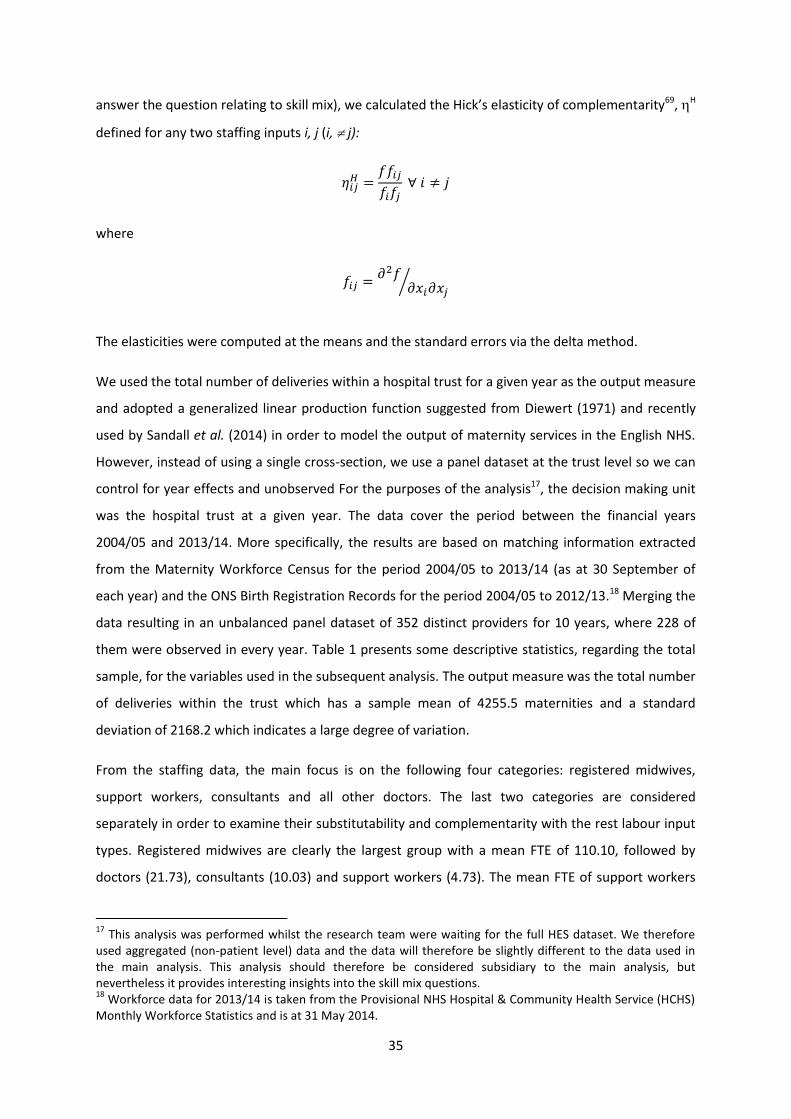
answer the question relating to skill mix), we calculated the Hick’s elasticity of complementarity69, H

defined for any two staffing inputs i, j (i, j):

𝜂𝑖𝑗𝐻 =

𝑓𝑓𝑖𝑗

𝑓𝑖𝑓𝑗 ∀ 𝑖 ≠ 𝑗

where

𝑓𝑖𝑗 =𝜕2𝑓

𝜕𝑥𝑖𝜕𝑥𝑗⁄

The elasticities were computed at the means and the standard errors via the delta method.

We used the total number of deliveries within a hospital trust for a given year as the output measure

and adopted a generalized linear production function suggested from Diewert (1971) and recently

used by Sandall et al. (2014) in order to model the output of maternity services in the English NHS.

However, instead of using a single cross-section, we use a panel dataset at the trust level so we can

control for year effects and unobserved For the purposes of the analysis17, the decision making unit

was the hospital trust at a given year. The data cover the period between the financial years

2004/05 and 2013/14. More specifically, the results are based on matching information extracted

from the Maternity Workforce Census for the period 2004/05 to 2013/14 (as at 30 September of

each year) and the ONS Birth Registration Records for the period 2004/05 to 2012/13.18 Merging the

data resulting in an unbalanced panel dataset of 352 distinct providers for 10 years, where 228 of

them were observed in every year. Table 1 presents some descriptive statistics, regarding the total

sample, for the variables used in the subsequent analysis. The output measure was the total number

of deliveries within the trust which has a sample mean of 4255.5 maternities and a standard

deviation of 2168.2 which indicates a large degree of variation.

From the staffing data, the main focus is on the following four categories: registered midwives,

support workers, consultants and all other doctors. The last two categories are considered

separately in order to examine their substitutability and complementarity with the rest labour input

types. Registered midwives are clearly the largest group with a mean FTE of 110.10, followed by

doctors (21.73), consultants (10.03) and support workers (4.73). The mean FTE of support workers

17

This analysis was performed whilst the research team were waiting for the full HES dataset. We therefore used aggregated (non-patient level) data and the data will therefore be slightly different to the data used in the main analysis. This analysis should therefore be considered subsidiary to the main analysis, but nevertheless it provides interesting insights into the skill mix questions. 18

Workforce data for 2013/14 is taken from the Provisional NHS Hospital & Community Health Service (HCHS) Monthly Workforce Statistics and is at 31 May 2014.

36

may seem small, however, a simple descriptive analysis indicates that their use has been following a

steadily upward trend during the period under investigation, from a mean FTE of 2.99 in 2004/05 to

a mean FTE of 7.31 in 2013/14. The evolution in the use of doctors and consultants has been rather

stable throughout the total period while the mean FTE of registered midwives has been increased

from 97.37 in 2004/05 to 132.05 in 2013/14. The data are therefore comparable to that used in the

main statistical analysis.

37

4 Results

4.1 Statistical Analysis

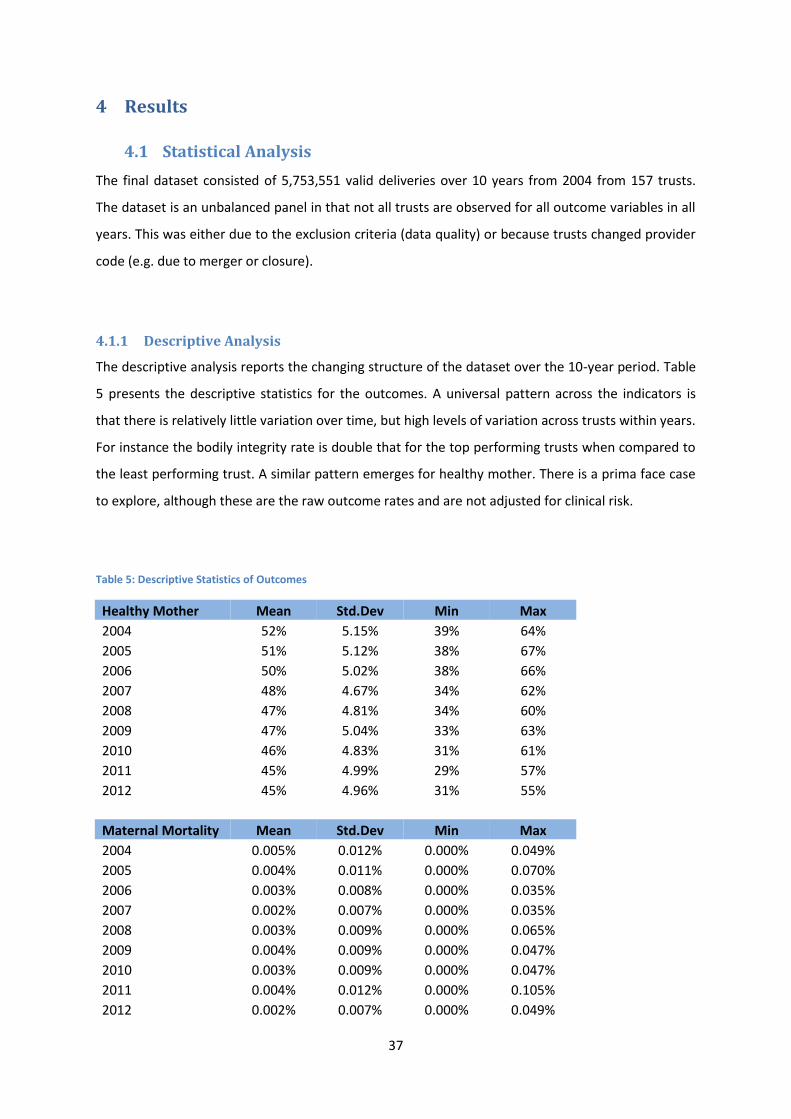
The final dataset consisted of 5,753,551 valid deliveries over 10 years from 2004 from 157 trusts.

The dataset is an unbalanced panel in that not all trusts are observed for all outcome variables in all

years. This was either due to the exclusion criteria (data quality) or because trusts changed provider

code (e.g. due to merger or closure).

4.1.1 Descriptive Analysis

The descriptive analysis reports the changing structure of the dataset over the 10-year period. Table

5 presents the descriptive statistics for the outcomes. A universal pattern across the indicators is

that there is relatively little variation over time, but high levels of variation across trusts within years.

For instance the bodily integrity rate is double that for the top performing trusts when compared to

the least performing trust. A similar pattern emerges for healthy mother. There is a prima face case

to explore, although these are the raw outcome rates and are not adjusted for clinical risk.

Table 5: Descriptive Statistics of Outcomes

Healthy Mother Mean Std.Dev Min Max

2004 52% 5.15% 39% 64%

2005 51% 5.12% 38% 67%

2006 50% 5.02% 38% 66%

2007 48% 4.67% 34% 62%

2008 47% 4.81% 34% 60%

2009 47% 5.04% 33% 63%

2010 46% 4.83% 31% 61%

2011 45% 4.99% 29% 57%

2012 45% 4.96% 31% 55%

Maternal Mortality Mean Std.Dev Min Max

2004 0.005% 0.012% 0.000% 0.049%

2005 0.004% 0.011% 0.000% 0.070%

2006 0.003% 0.008% 0.000% 0.035%

2007 0.002% 0.007% 0.000% 0.035%

2008 0.003% 0.009% 0.000% 0.065%

2009 0.004% 0.009% 0.000% 0.047%

2010 0.003% 0.009% 0.000% 0.047%

2011 0.004% 0.012% 0.000% 0.105%

2012 0.002% 0.007% 0.000% 0.049%

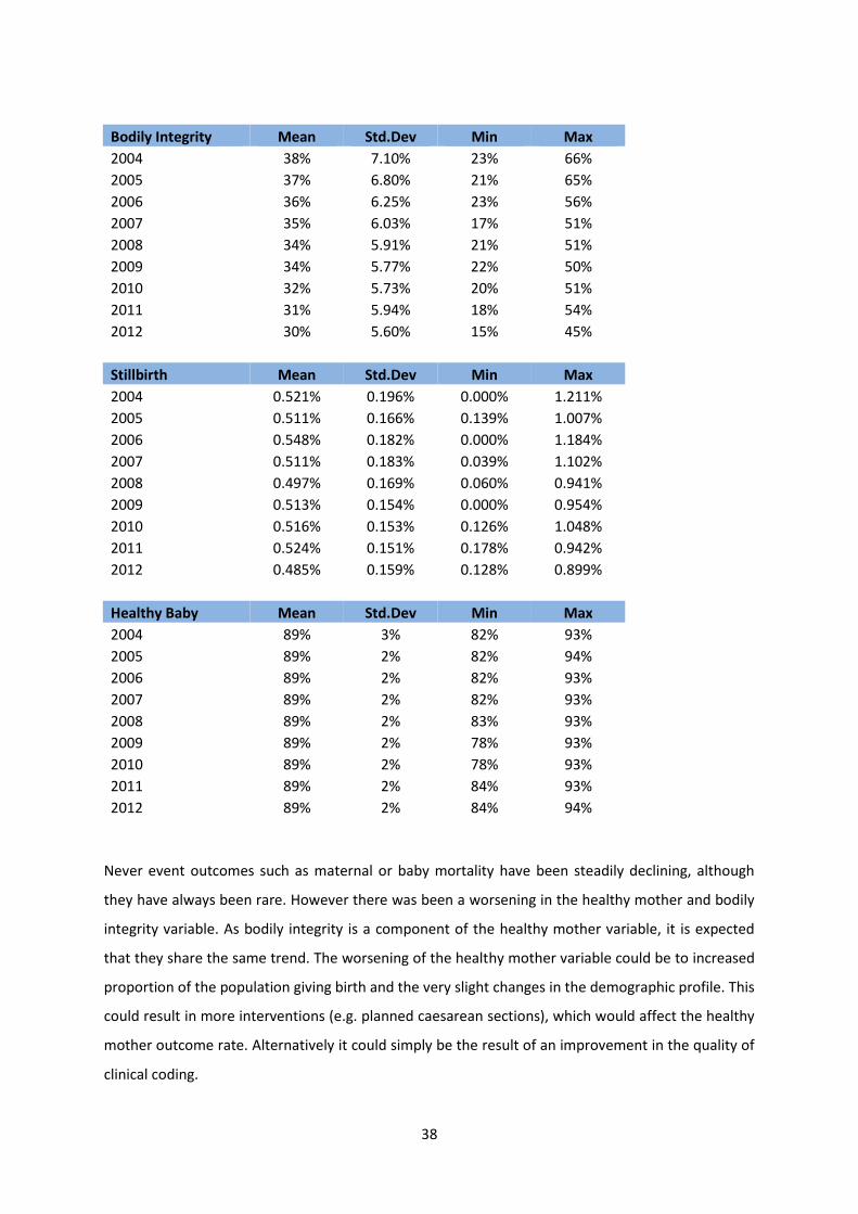
38

Bodily Integrity Mean Std.Dev Min Max

2004 38% 7.10% 23% 66%

2005 37% 6.80% 21% 65%

2006 36% 6.25% 23% 56%

2007 35% 6.03% 17% 51%

2008 34% 5.91% 21% 51%

2009 34% 5.77% 22% 50%

2010 32% 5.73% 20% 51%

2011 31% 5.94% 18% 54%

2012 30% 5.60% 15% 45%

Stillbirth Mean Std.Dev Min Max

2004 0.521% 0.196% 0.000% 1.211%

2005 0.511% 0.166% 0.139% 1.007%

2006 0.548% 0.182% 0.000% 1.184%

2007 0.511% 0.183% 0.039% 1.102%

2008 0.497% 0.169% 0.060% 0.941%

2009 0.513% 0.154% 0.000% 0.954%

2010 0.516% 0.153% 0.126% 1.048%

2011 0.524% 0.151% 0.178% 0.942%

2012 0.485% 0.159% 0.128% 0.899%

Healthy Baby Mean Std.Dev Min Max

2004 89% 3% 82% 93%

2005 89% 2% 82% 94%

2006 89% 2% 82% 93%

2007 89% 2% 82% 93%

2008 89% 2% 83% 93%

2009 89% 2% 78% 93%

2010 89% 2% 78% 93%

2011 89% 2% 84% 93%

2012 89% 2% 84% 94%

Never event outcomes such as maternal or baby mortality have been steadily declining, although

they have always been rare. However there was been a worsening in the healthy mother and bodily

integrity variable. As bodily integrity is a component of the healthy mother variable, it is expected

that they share the same trend. The worsening of the healthy mother variable could be to increased

proportion of the population giving birth and the very slight changes in the demographic profile. This

could result in more interventions (e.g. planned caesarean sections), which would affect the healthy

mother outcome rate. Alternatively it could simply be the result of an improvement in the quality of

clinical coding.

39

As the statistics in Table 6 illustrate, there is remarkably little variation in the profile of woman giving

birth over the past decade with respect to all of the variables except clinical risk which has increased

from 41% in 2004 to 53% in 2013. This could, in part, be explained by an improvement in the level of

clinical coding of particular conditions or procedures that would render a woman at “higher risk” of

a difficult delivery. Further, the age profile has altered very slightly with both a greater proportion of

younger and older woman giving birth. Whilst the statistical models will include fixed time effects to

test whether there is a time trend in the data (equivalent to estimating a different intercept or

baseline for each year), it is unlikely to provide much explanatory power. The SHA of each trusts

remains constant over the period and therefore only one observation is presented. However, the

substantial variation in outcomes across trends may be the result of variations in the case-mix or by

variations in hospital level factors such as staffing. The multilevel modelling introduced in Section

3.3.2 will allow for this to be tested and for the effect of both individual (patient level) and group

(trust level) predictors to determine the outcomes.

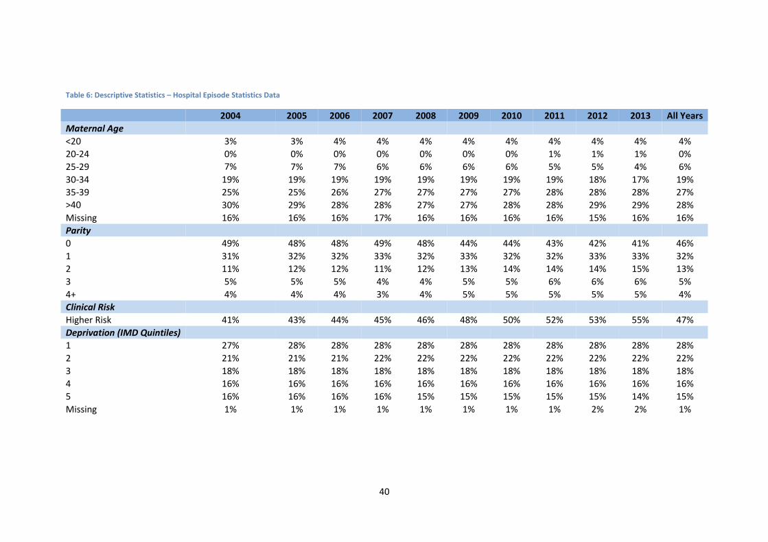
40

Table 6: Descriptive Statistics – Hospital Episode Statistics Data

2004 2005 2006 2007 2008 2009 2010 2011 2012 2013 All Years

Maternal Age

<20 3% 3% 4% 4% 4% 4% 4% 4% 4% 4% 4%

20-24 0% 0% 0% 0% 0% 0% 0% 1% 1% 1% 0%

25-29 7% 7% 7% 6% 6% 6% 6% 5% 5% 4% 6%

30-34 19% 19% 19% 19% 19% 19% 19% 19% 18% 17% 19%

35-39 25% 25% 26% 27% 27% 27% 27% 28% 28% 28% 27%

>40 30% 29% 28% 28% 27% 27% 28% 28% 29% 29% 28%

Missing 16% 16% 16% 17% 16% 16% 16% 16% 15% 16% 16%

Parity

0 49% 48% 48% 49% 48% 44% 44% 43% 42% 41% 46%

1 31% 32% 32% 33% 32% 33% 32% 32% 33% 33% 32%

2 11% 12% 12% 11% 12% 13% 14% 14% 14% 15% 13%

3 5% 5% 5% 4% 4% 5% 5% 6% 6% 6% 5%

4+ 4% 4% 4% 3% 4% 5% 5% 5% 5% 5% 4%

Clinical Risk

Higher Risk 41% 43% 44% 45% 46% 48% 50% 52% 53% 55% 47%

Deprivation (IMD Quintiles)

1 27% 28% 28% 28% 28% 28% 28% 28% 28% 28% 28%

2 21% 21% 21% 22% 22% 22% 22% 22% 22% 22% 22%

3 18% 18% 18% 18% 18% 18% 18% 18% 18% 18% 18%

4 16% 16% 16% 16% 16% 16% 16% 16% 16% 16% 16%

5 16% 16% 16% 16% 15% 15% 15% 15% 15% 14% 15%

Missing 1% 1% 1% 1% 1% 1% 1% 1% 2% 2% 1%

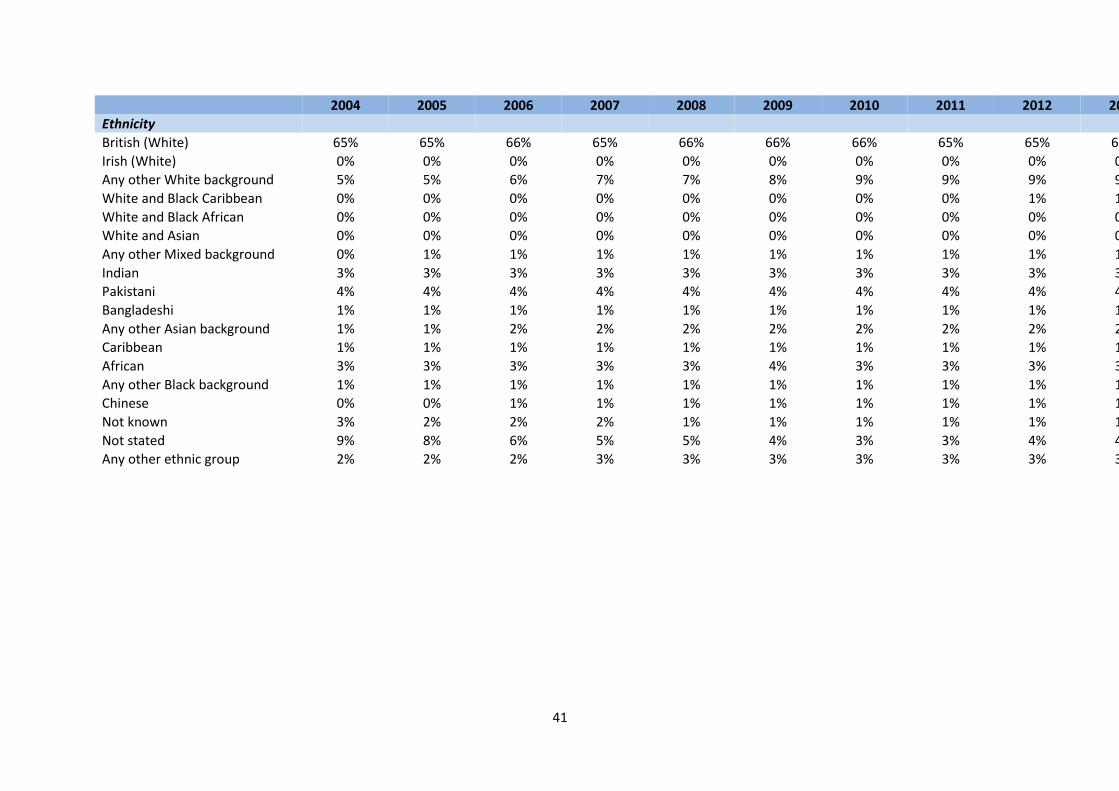
41

2004 2005 2006 2007 2008 2009 2010 2011 2012 2013 All Years

Ethnicity

British (White) 65% 65% 66% 65% 66% 66% 66% 65% 65% 64% 65%

Irish (White) 0% 0% 0% 0% 0% 0% 0% 0% 0% 0% 0%

Any other White background 5% 5% 6% 7% 7% 8% 9% 9% 9% 9% 7%

White and Black Caribbean 0% 0% 0% 0% 0% 0% 0% 0% 1% 1% 0%

White and Black African 0% 0% 0% 0% 0% 0% 0% 0% 0% 0% 0%

White and Asian 0% 0% 0% 0% 0% 0% 0% 0% 0% 0% 0%

Any other Mixed background 0% 1% 1% 1% 1% 1% 1% 1% 1% 1% 1%

Indian 3% 3% 3% 3% 3% 3% 3% 3% 3% 3% 3%

Pakistani 4% 4% 4% 4% 4% 4% 4% 4% 4% 4% 4%

Bangladeshi 1% 1% 1% 1% 1% 1% 1% 1% 1% 1% 1%

Any other Asian background 1% 1% 2% 2% 2% 2% 2% 2% 2% 2% 2%

Caribbean 1% 1% 1% 1% 1% 1% 1% 1% 1% 1% 1%

African 3% 3% 3% 3% 3% 4% 3% 3% 3% 3% 3%

Any other Black background 1% 1% 1% 1% 1% 1% 1% 1% 1% 1% 1%

Chinese 0% 0% 1% 1% 1% 1% 1% 1% 1% 1% 1%

Not known 3% 2% 2% 2% 1% 1% 1% 1% 1% 1% 1%

Not stated 9% 8% 6% 5% 5% 4% 3% 3% 4% 4% 5%

Any other ethnic group 2% 2% 2% 3% 3% 3% 3% 3% 3% 3% 3%

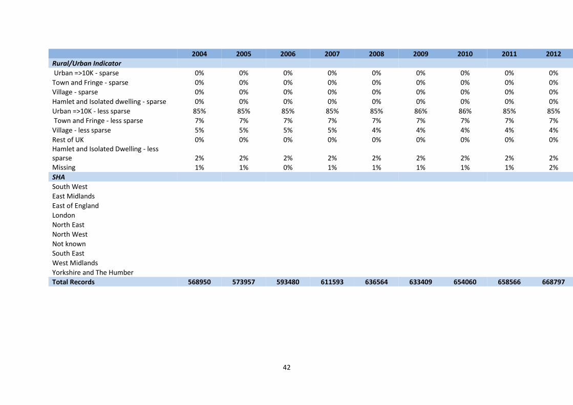
42

2004 2005 2006 2007 2008 2009 2010 2011 2012 2013 All Years

Rural/Urban Indicator

Urban =>10K - sparse 0% 0% 0% 0% 0% 0% 0% 0% 0% 0% 0%

Town and Fringe - sparse 0% 0% 0% 0% 0% 0% 0% 0% 0% 0% 0%

Village - sparse 0% 0% 0% 0% 0% 0% 0% 0% 0% 0% 0%

Hamlet and Isolated dwelling - sparse 0% 0% 0% 0% 0% 0% 0% 0% 0% 0% 0%

Urban =>10K - less sparse 85% 85% 85% 85% 85% 86% 86% 85% 85% 84% 85%

Town and Fringe - less sparse 7% 7% 7% 7% 7% 7% 7% 7% 7% 7% 7%

Village - less sparse 5% 5% 5% 5% 4% 4% 4% 4% 4% 4% 5%

Rest of UK 0% 0% 0% 0% 0% 0% 0% 0% 0% 0% 0% Hamlet and Isolated Dwelling - less sparse 2% 2% 2% 2% 2% 2% 2% 2% 2% 2% 2% Missing 1% 1% 0% 1% 1% 1% 1% 1% 2% 2% 1%

SHA

South West

10%

East Midlands

6%

East of England

11%

London

19%

North East

5%

North West

14%

Not known

0%

South East

15%

West Midlands

10%

Yorkshire and The Humber

9%

Total Records 568950 573957 593480 611593 636564 633409 654060 658566 668797 154180 5753556

43

4.1.1.1 Staffing Trends

Table 7 presents some descriptive statistics on the staffing data. Again, there is relatively little

variation in the average number of staff per 100 deliveries for each of the staffing groups over the

decade, but greater variation within a year across trusts. The minimum and maximum values, whilst

plausible, are very far apart and the standard deviation is relatively high. For example in 2013 the

range of registered midwives per 100 deliveries is 1.55-16.71. This points to a fair degree of trust

level variation in the staff to patient ratio. Recall, however, that this represents the total number of

these staff (e.g. registered midwives) in the whole trust and there may be variation across trusts in

how these staff are deployed across different maternity services, wards or between obstetrics and

gynaecology. It also doesn’t capture differences in service configuration e.g. obstetric-led versus

midwife-led units. This is one of the major limitations of these aggregate data.

Comparing the data in Table 6 with those reported in Sandall et al. (2014) they are broadly similar

despite the dataset being slightly different. Similarly to the HES patient level data described in the

previous section, there is a strong correlation between these figures and those reported in Sandall et

al. (2014). For instance, the 2010 FTE midwives per 100 deliveries is 3.10 in this study and 3.08 in

Sandall et al. (2014).

A descriptive analysis of trends in staffing levels and skill mix variables over the decade to 2013

provides some interesting insights for the following variables:

1. FTE doctors per 100 maternities

2. FTE midwives per 100 maternities

3. FTE support workers per 100 maternities

4. FTE all staff per 100 maternities

5. FTE managers per 100 maternities

6. Doctors to midwives ratio

7. Support workers to midwives ratio

8. Managers to total staff ratio

To understand the variation between regions, the trust level data were collapsed by year and Strategic Health Authority (SHA), and each index is plotted separately for each one of the ten SHAs as well as for the country as a whole. The yellow curve superimposed on each plot is a 3

rd degree polynomial which smooths out the general trend. Unlike the

data reported in Table 7, the following figures describe the full sample of staffing data including trusts which were excluded from the statistical analysis (either as a result of poor quality coding or due to a lack of matching) and primary care trusts. Primary trusts provide a great deal of community based midwifery care (e.g. antenatal care and home deliveries), which will distort the representation somewhat. Figure 2: FTE Registered Midwives per 100 Maternities 2003-2013

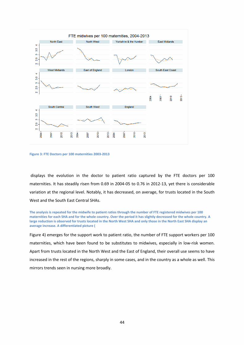
44

Figure 3: FTE Doctors per 100 maternities 2003-2013

displays the evolution in the doctor to patient ratio captured by the FTE doctors per 100

maternities. It has steadily risen from 0.69 in 2004-05 to 0.76 in 2012-13, yet there is considerable

variation at the regional level. Notably, it has decreased, on average, for trusts located in the South

West and the South East Central SHAs.

The analysis is repeated for the midwife to patient ratios through the number of FTE registered midwives per 100 maternities for each SHA and for the whole country. Over the period it has slightly decreased for the whole country. A large reduction is observed for trusts located in the North West SHA and only those in the North East SHA display an average increase. A differentiated picture (

Figure 4) emerges for the support work to patient ratio, the number of FTE support workers per 100

maternities, which have been found to be substitutes to midwives, especially in low-risk women.

Apart from trusts located in the North West and the East of England, their overall use seems to have

increased in the rest of the regions, sharply in some cases, and in the country as a whole as well. This

mirrors trends seen in nursing more broadly.

45

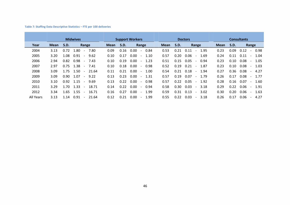
46

Table 7: Staffing Data Descriptive Statistics – FTE per 100 deliveries

Midwives Support Workers Doctors Consultants

Year Mean S.D. Range Mean S.D. Range Mean S.D. Range Mean S.D. Range

2004 3.13 0.72 1.80 - 7.80

0.09 0.16 0.00 - 0.84

0.53 0.21 0.11 - 1.95

0.23 0.09 0.12 - 0.98

2005 3.20 1.08 0.91 - 9.62

0.10 0.17 0.00 - 1.10

0.57 0.20 0.06 - 1.69

0.24 0.11 0.11 - 1.04

2006 2.94 0.82 0.98 - 7.43

0.10 0.19 0.00 - 1.23

0.51 0.15 0.05 - 0.94

0.23 0.10 0.08 - 1.05

2007 2.97 0.75 1.38 - 7.41

0.10 0.18 0.00 - 0.98

0.52 0.19 0.21 - 1.87

0.23 0.10 0.08 - 1.03

2008 3.09 1.75 1.50 - 21.64

0.11 0.21 0.00 - 1.00

0.54 0.21 0.18 - 1.94

0.27 0.36 0.08 - 4.27

2009 3.09 0.90 1.07 - 9.22

0.13 0.23 0.00 - 1.31

0.57 0.19 0.07 - 1.79

0.26 0.17 0.08 - 1.77

2010 3.10 0.92 1.15 - 9.69

0.13 0.22 0.00 - 0.98

0.57 0.22 0.05 - 1.92

0.28 0.16 0.07 - 1.60

2011 3.29 1.70 1.33 - 18.71

0.14 0.22 0.00 - 0.94

0.58 0.30 0.03 - 3.18

0.29 0.22 0.06 - 1.91

2012 3.34 1.65 1.55 - 16.71

0.16 0.27 0.00 - 1.99

0.59 0.31 0.13 - 3.02

0.30 0.20 0.06 - 1.63

All Years 3.13 1.14 0.91 - 21.64

0.12 0.21 0.00 - 1.99

0.55 0.22 0.03 - 3.18

0.26 0.17 0.06 - 4.27

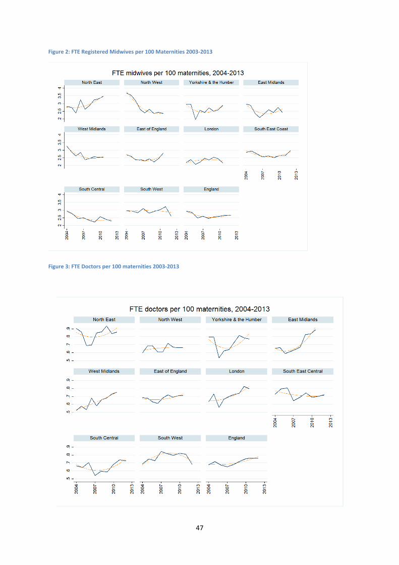
47

Figure 2: FTE Registered Midwives per 100 Maternities 2003-2013

Figure 3: FTE Doctors per 100 maternities 2003-2013

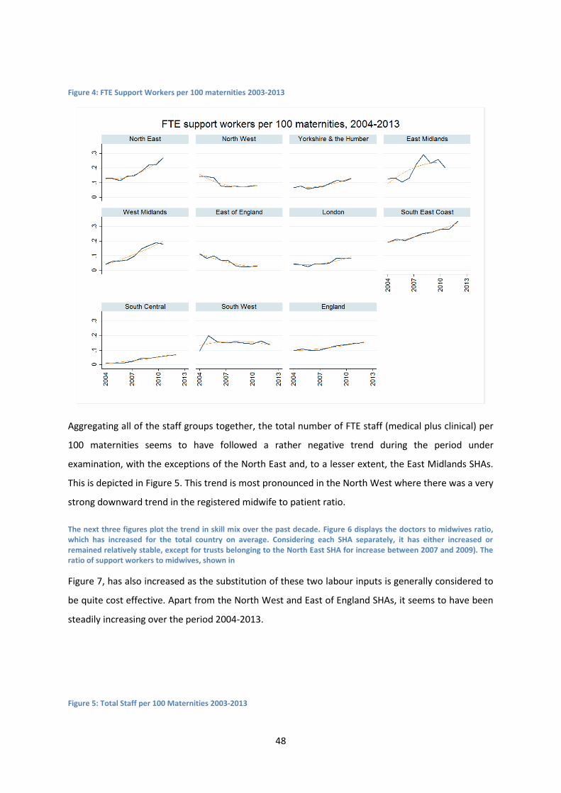
48

Figure 4: FTE Support Workers per 100 maternities 2003-2013

Aggregating all of the staff groups together, the total number of FTE staff (medical plus clinical) per

100 maternities seems to have followed a rather negative trend during the period under

examination, with the exceptions of the North East and, to a lesser extent, the East Midlands SHAs.

This is depicted in Figure 5. This trend is most pronounced in the North West where there was a very

strong downward trend in the registered midwife to patient ratio.

The next three figures plot the trend in skill mix over the past decade. Figure 6 displays the doctors to midwives ratio, which has increased for the total country on average. Considering each SHA separately, it has either increased or remained relatively stable, except for trusts belonging to the North East SHA for increase between 2007 and 2009). The ratio of support workers to midwives, shown in

Figure 7, has also increased as the substitution of these two labour inputs is generally considered to

be quite cost effective. Apart from the North West and East of England SHAs, it seems to have been

steadily increasing over the period 2004-2013.

Figure 5: Total Staff per 100 Maternities 2003-2013

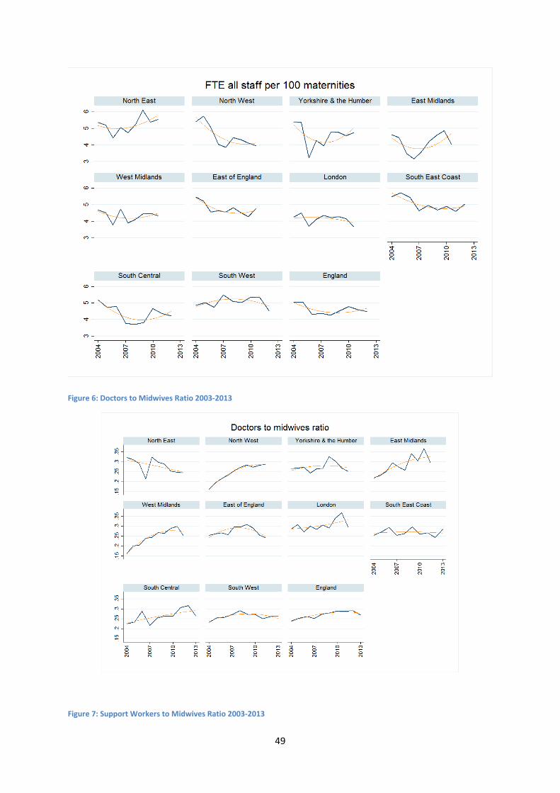
49

Figure 6: Doctors to Midwives Ratio 2003-2013

Figure 7: Support Workers to Midwives Ratio 2003-2013

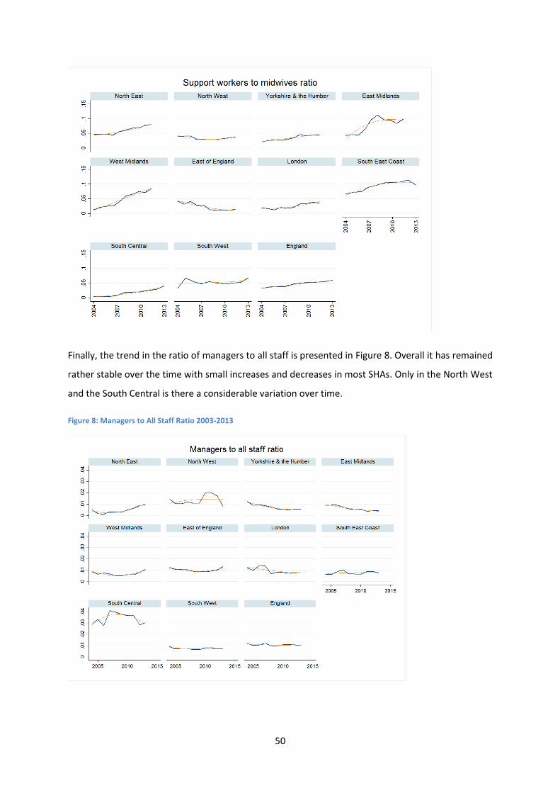
50

Finally, the trend in the ratio of managers to all staff is presented in Figure 8. Overall it has remained

rather stable over the time with small increases and decreases in most SHAs. Only in the North West

and the South Central is there a considerable variation over time.

Figure 8: Managers to All Staff Ratio 2003-2013

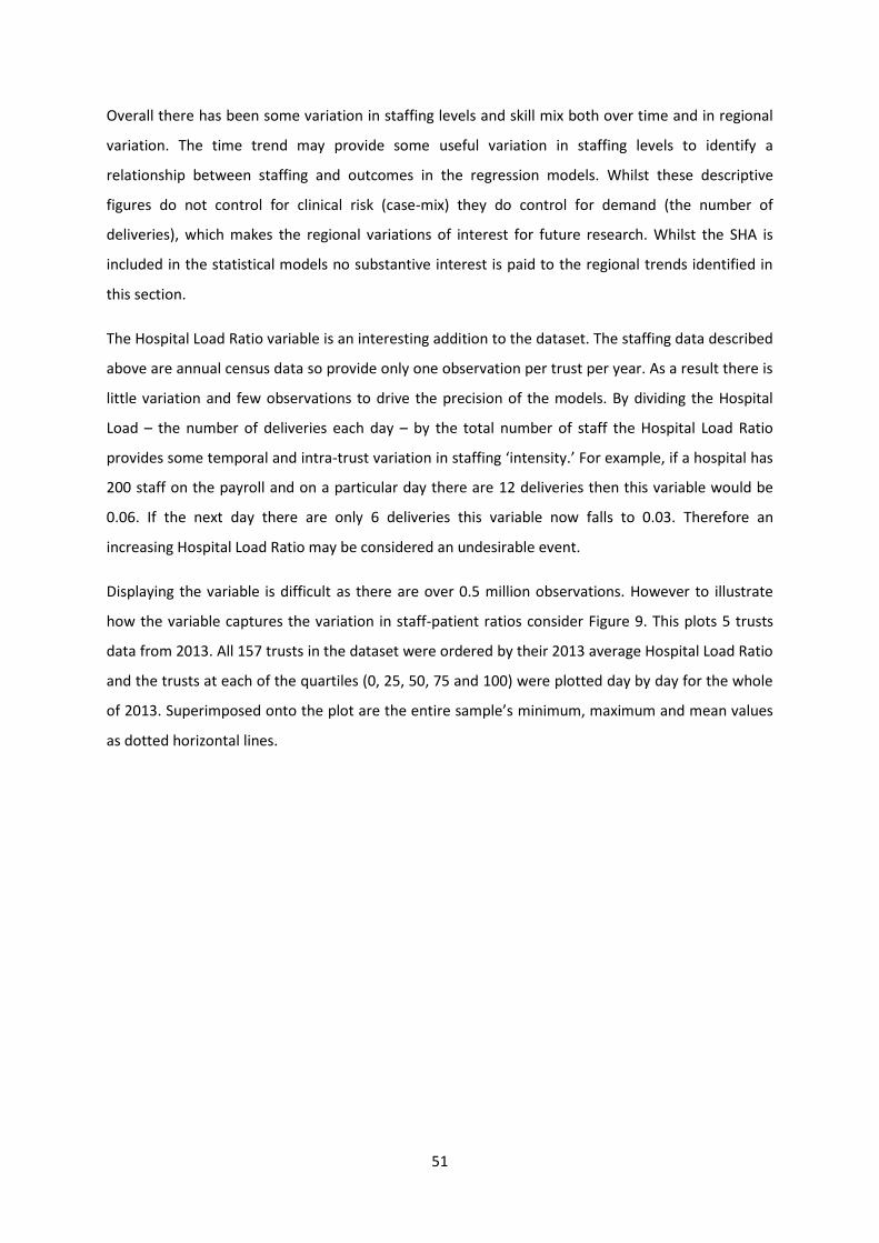
51

Overall there has been some variation in staffing levels and skill mix both over time and in regional

variation. The time trend may provide some useful variation in staffing levels to identify a

relationship between staffing and outcomes in the regression models. Whilst these descriptive

figures do not control for clinical risk (case-mix) they do control for demand (the number of

deliveries), which makes the regional variations of interest for future research. Whilst the SHA is

included in the statistical models no substantive interest is paid to the regional trends identified in

this section.

The Hospital Load Ratio variable is an interesting addition to the dataset. The staffing data described

above are annual census data so provide only one observation per trust per year. As a result there is

little variation and few observations to drive the precision of the models. By dividing the Hospital

Load – the number of deliveries each day – by the total number of staff the Hospital Load Ratio

provides some temporal and intra-trust variation in staffing ‘intensity.’ For example, if a hospital has

200 staff on the payroll and on a particular day there are 12 deliveries then this variable would be

0.06. If the next day there are only 6 deliveries this variable now falls to 0.03. Therefore an

increasing Hospital Load Ratio may be considered an undesirable event.

Displaying the variable is difficult as there are over 0.5 million observations. However to illustrate

how the variable captures the variation in staff-patient ratios consider Figure 9. This plots 5 trusts

data from 2013. All 157 trusts in the dataset were ordered by their 2013 average Hospital Load Ratio

and the trusts at each of the quartiles (0, 25, 50, 75 and 100) were plotted day by day for the whole

of 2013. Superimposed onto the plot are the entire sample’s minimum, maximum and mean values

as dotted horizontal lines.

52

Figure 9: Hospital Load Ratio Variation 2013

4.1.2 Statistical (Regression) Results

Multilevel models were fitted to the data as described in Section 3.3.2 in detail. Whilst the models

took a relatively long time to be estimated due to their complexity and the choice of an optimization

algorithm that favoured precision over speed, the fitted models had good convergence properties.

The following tables present a simplified set of results for the statistical analysis, presenting the

findings of relevance for the economic evaluation. Full results are reserved to the appendix for

interested readers.

Logistic regression models to outcomes using the logit function, that is the log of the odds of the

outcome. It is more common to exponeniate the regression (beta) coefficients to produce odds

ratios. For categorical variables such as clinical risk, the interpretation is easy. The odds ratio is the

difference in the odds of the outcomes between the categories of the variable. For instance, if the

odds ratio for higher risk for maternal mortality was 2 then mothers in the higher risk category are

twice as likely to die than those in the lower risk category. Odds ratios (OR) also provide a way of

categorising the strength of association between multiple explanatory variables: strong (OR > 3),

moderate (OR = 1.6-3.0), or weak (OR=1.1-1.5). Attention is therefore focused on the odds ratio.

The statistical significance of the variables can be determined in two ways. Firstly, asterisks indicate

whether the estimated p-value of each coefficient is less than 10 per cent (*), 5 per cent (**) or 1

53

per cent (***). The standard errors, t-statistics and actual p-values are reported in full in the

appendix. Caution should be used when relying solely on the p-values as the standard errors are

unreliable as discussed in the methods section. Secondly, the results of the Likelihood Ratio tests are

reported as Chi-Squared tests at the foot of each regression model. This tests the statistical

significance of the improvement in the model fit of adding groups of coefficients to the model.

Very few of the explanatory variables were statistically significant in the maternal mortality model,

although the AUC was quite high (0.76) indicating that the model was able to discriminate cases.

Clinical risk has the largest effect, with mothers in the higher risk category 4.25 times more likely to

die than those in the lower risk category. It should be stressed that this is from a very low

unconditional probability of death of 0.002% on average. Maternal age was also an important

predictor of maternal death, with mothers aged 25-35 approximately half as likely to die than those

aged over 40. For women under 25 they were less than a third as likely to die than those aged over

40. Some of the ethnicity categories were statistically significant predictors with large odds ratios.

However as they are marginally statistically significant despite their large regression coefficients and

given the approximate nature of the standard errors in the model, too much confidence should not

be placed in this finding unless strongly supported by theory.

The healthy mother and bodily integrity outcomes have very similar regression results. This is not

surprising as bodily integrity is a component indicator of healthy mother. There is a clear time

dimension to the results, with each year being strongly significantly related to the outcome. When

compared to 2004 (the base year) each year since has a lower rate of healthy mothers and bodily

integrity. This was also clear in the descriptive statistics in Section 4.1.1. For instance, a mother

giving birth in 2012 is more than 30% less likely to be “healthy” or have “bodily integrity” than those

giving birth in 2004.

Patient level factors are clearly very important, with age, ethnicity and parity being associated with

both outcomes and deprivation also being associated with bodily integrity. In both cases, the largest

odds ratio is for the clinical risk variable. A mother classed as “higher risk” is half as likely to deliver

with bodily integrity than a mother classed as “lower risk”.

In terms of the trust level variables, larger trusts have lower healthy mother rates but this effect is

weak. The association between support worker staffing levels and both outcomes is marginal both in

terms of effect size and statistical significance. There is a stronger relationship between medical staff

(both junior doctors and consultants) and both outcomes. This is to be expected but the relationship

could be reverse causal. Trusts that perform more planned caesareans for example will require more

consultants, ceteris paribus, but will by definition have lower healthy mother and bodily integrity

54

rates due to the procedure. Midwifery levels are positively associated with healthy mother and

bodily integrity rates but these relationships are weak (OR: 1.019 and 1.01). The statistical

significance of the findings likely comes from the very large dataset and the associated improvement

in precision.

All of these findings are congruent with those of the extant literature, especially with Sandall et al.

(2014); the difference in the statistical significance of the staffing variables being explained by the

larger sample. The most interesting and novel finding is with respect to the Hospital Load Ratio. This

variable was included to proxy the effect of shift-by-shift variation in staff to patient ratios. As no

staffing data are available at this level or frequency, the variation in “demand” was exploited under

the assumption of constant staffing levels to create variation in the staff to patient ratios. Whilst

interpretation of the variable is impossible, days in which there are higher patient loads have much

worse outcomes. The odds ratio is strong and statistically significant for healthy mother.

This may be the subtle but important difference between staffing levels and skill mix which may be a

fruitful avenue for future research. For instance, a low ratio of staff to patients on a shift-by-shift

basis, caused either by staff shortage or excess patients, may result in poorer outcomes for mothers.

This may lead to complications such as, inter alia, maternal sepsis or other problems that result in

longer lengths of stay or readmission. However, skill mix which wasn’t captured in this pseudo shift

level variable may be the critical factor in outcomes relating to interventionist procedures such as

caesarean sections or episiotomy. At present this must be left as a hypothesis for further research

but it is a possible explanation for the finding.

Confusingly there is an inverse relationship with both bodily integrity (a subset of healthy mother)

and healthy baby outcomes. However, the statistical significance is marginal and these findings may

be the result of underestimated standard errors as discussed in the methodology section. The odds

ratios are also relatively weak (healthy baby = 1.32; bodily integrity = 1.16). Yet at present the

findings cannot be discounted. For these two outcomes therefore a worsening Hospital Load Ratio

would improve outcomes.

Neither baby outcomes were significantly associated with midwifery staffing levels. However higher

levels of support workers (ceteris paribus) was associated with lower healthy baby rates whilst

higher consultant and doctor staffing levels were associated with higher healthy baby rates. As per

the maternal outcomes, there was a clear association between maternal age, clinical risk, ethnicity

and parity and both baby outcomes. Yet again, clinical risk had the largest odds ratios, with a mother

classified as higher risk being 32 times more likely to have a stillborn baby than lower risk mothers.

Unlike the other regression models, area deprivation and the geographic variables (SHA and

55

rural/urban classification) were statistically significant predictors of the baby outcomes. Compared

to the South West for example, each other SHA was 30-50% more likely to have a healthy baby.

In all cases the AUC statistics indicate that the models had good discriminatory properties and

correctly identify outcomes most of the time. With the exception of the healthy mother indicator

(AUC = 0.67), the AUC were high (>0.7) and for healthy baby it was very high (AUC = 0.81). In every

model the variation in the outcome attributed to the trust is less than 2% with 98-99% of the

variance in the outcomes due to mothers’ characteristics. Therefore as staffing is determine at the

trust level it is unlikely to have a large effect on the outcomes.

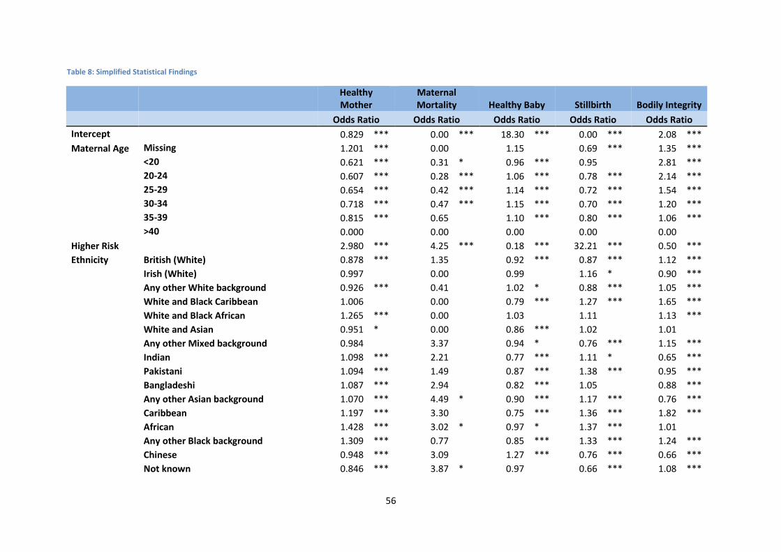
56

Table 8: Simplified Statistical Findings

Healthy Mother

Maternal Mortality Healthy Baby Stillbirth Bodily Integrity

Odds Ratio Odds Ratio Odds Ratio Odds Ratio Odds Ratio

Intercept

0.829 *** 0.00 *** 18.30 *** 0.00 *** 2.08 ***

Maternal Age Missing 1.201 *** 0.00

1.15

0.69 *** 1.35 ***

<20 0.621 *** 0.31 * 0.96 *** 0.95

2.81 ***

20-24 0.607 *** 0.28 *** 1.06 *** 0.78 *** 2.14 ***

25-29 0.654 *** 0.42 *** 1.14 *** 0.72 *** 1.54 ***

30-34 0.718 *** 0.47 *** 1.15 *** 0.70 *** 1.20 ***

35-39 0.815 *** 0.65

1.10 *** 0.80 *** 1.06 ***

>40 0.000

0.00

0.00

0.00

0.00 Higher Risk

2.980 *** 4.25 *** 0.18 *** 32.21 *** 0.50 ***

Ethnicity British (White) 0.878 *** 1.35

0.92 *** 0.87 *** 1.12 ***

Irish (White) 0.997

0.00

0.99

1.16 * 0.90 ***

Any other White background 0.926 *** 0.41

1.02 * 0.88 *** 1.05 ***

White and Black Caribbean 1.006

0.00

0.79 *** 1.27 *** 1.65 ***

White and Black African 1.265 *** 0.00

1.03

1.11

1.13 ***

White and Asian 0.951 * 0.00

0.86 *** 1.02

1.01

Any other Mixed background 0.984

3.37

0.94 * 0.76 *** 1.15 ***

Indian 1.098 *** 2.21

0.77 *** 1.11 * 0.65 ***

Pakistani 1.094 *** 1.49

0.87 *** 1.38 *** 0.95 ***

Bangladeshi 1.087 *** 2.94

0.82 *** 1.05

0.88 ***

Any other Asian background 1.070 *** 4.49 * 0.90 *** 1.17 *** 0.76 ***

Caribbean 1.197 *** 3.30

0.75 *** 1.36 *** 1.82 ***

African 1.428 *** 3.02 * 0.97 * 1.37 *** 1.01

Any other Black background 1.309 *** 0.77

0.85 *** 1.33 *** 1.24 ***

Chinese 0.948 *** 3.09

1.27 *** 0.76 *** 0.66 ***

Not known 0.846 *** 3.87 * 0.97

0.66 *** 1.08 ***

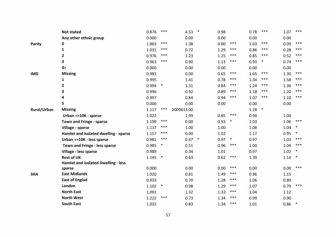
57

Not stated 0.876 *** 4.53 * 0.98

0.78 *** 1.07 ***

Any other ethnic group 0.000

0.00

0.00

0.00

0.00

Parity 0 1.863 *** 1.38

0.80 *** 1.63 *** 0.09 ***

1 1.031 *** 0.72

1.29 *** 0.86 *** 0.28 ***

2 0.976 *** 1.23

1.25 *** 0.85 *** 0.52 ***

3 0.963 *** 0.90

1.13 *** 0.93 * 0.74 ***

4> 0.000

0.00

0.00

0.00

0.00 IMD Missing 0.983

0.00

0.65 *** 1.65 *** 1.30 ***

1 0.995

1.41

0.78 *** 1.34 *** 1.58 ***

2 0.994 * 1.31

0.84 *** 1.24 *** 1.36 ***

3 0.996

0.92

0.89 *** 1.18 *** 1.20 ***

4 0.997

0.84

0.94 *** 1.07 *** 1.10 ***

5 0.000

0.00

0.00

0.00

0.00 Rural/Urban Missing 1.117 *** 2009613.00

1.28 *

Urban =>10K - sparse 1.022

1.99

0.85 *** 0.94

1.04

Town and Fringe - sparse 1.199 *** 0.00

0.93 * 1.03

1.06 ***

Village - sparse 1.117 *** 1.00

1.00

1.08

1.04 *

Hamlet and Isolated dwelling - sparse 1.157 *** 0.00

1.02

1.17

0.95 *

Urban =>10K - less sparse 0.981 *** 0.47 * 0.97 * 0.97

1.03 ***

Town and Fringe - less sparse 0.985 * 0.51

0.96 *** 1.00

1.04 ***

Village - less sparse 0.989

0.34

1.01

0.97

1.02 *

Rest of UK 1.145 * 0.63

0.62 *** 1.39

1.14 *

Hamlet and Isolated Dwelling - less sparse 0.000

0.00

0.00 *** 0.00

0.00 ***

SHA East Midlands 1.020

0.81

1.49 *** 0.96

1.15

East of Englad 0.933

0.70

1.28 *** 1.06

0.89

London 1.102 * 0.98

1.29 *** 1.07

0.79 ***

North East 1.091

1.32

1.33 *** 1.04

1.12

North West 1.222 *** 0.73

1.34 *** 0.99

0.90

South East 1.032

0.83

1.34 *** 1.01

0.86 *

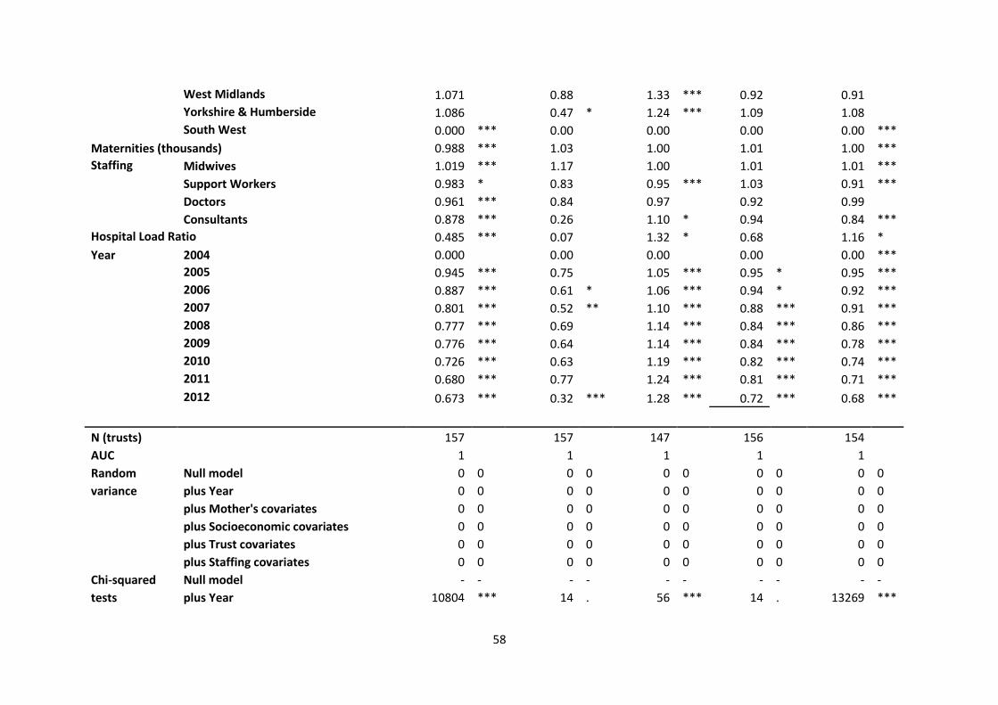
58

West Midlands 1.071

0.88

1.33 *** 0.92

0.91

Yorkshire & Humberside 1.086

0.47 * 1.24 *** 1.09

1.08

South West 0.000 *** 0.00

0.00

0.00

0.00 ***

Maternities (thousands) 0.988 *** 1.03

1.00

1.01

1.00 ***

Staffing Midwives 1.019 *** 1.17

1.00

1.01

1.01 ***

Support Workers 0.983 * 0.83

0.95 *** 1.03

0.91 ***

Doctors 0.961 *** 0.84

0.97

0.92

0.99

Consultants 0.878 *** 0.26

1.10 * 0.94

0.84 ***

Hospital Load Ratio 0.485 *** 0.07

1.32 * 0.68

1.16 *

Year 2004 0.000

0.00

0.00

0.00

0.00 ***

2005 0.945 *** 0.75

1.05 *** 0.95 * 0.95 ***

2006 0.887 *** 0.61 * 1.06 *** 0.94 * 0.92 ***

2007 0.801 *** 0.52 ** 1.10 *** 0.88 *** 0.91 ***

2008 0.777 *** 0.69

1.14 *** 0.84 *** 0.86 ***

2009 0.776 *** 0.64

1.14 *** 0.84 *** 0.78 ***

2010 0.726 *** 0.63

1.19 *** 0.82 *** 0.74 ***

2011 0.680 *** 0.77

1.24 *** 0.81 *** 0.71 ***

2012 0.673 *** 0.32 *** 1.28 *** 0.72 *** 0.68 ***

N (trusts)

157

157

147

156

154 AUC

1

1

1

1

1

Random Null model 0 0 0 0 0 0 0 0 0 0

variance plus Year 0 0 0 0 0 0 0 0 0 0

plus Mother's covariates 0 0 0 0 0 0 0 0 0 0

plus Socioeconomic covariates 0 0 0 0 0 0 0 0 0 0

plus Trust covariates 0 0 0 0 0 0 0 0 0 0

plus Staffing covariates 0 0 0 0 0 0 0 0 0 0

Chi-squared Null model - - - - - - - - - -

tests plus Year 10804 *** 14 . 56 *** 14 . 13269 ***

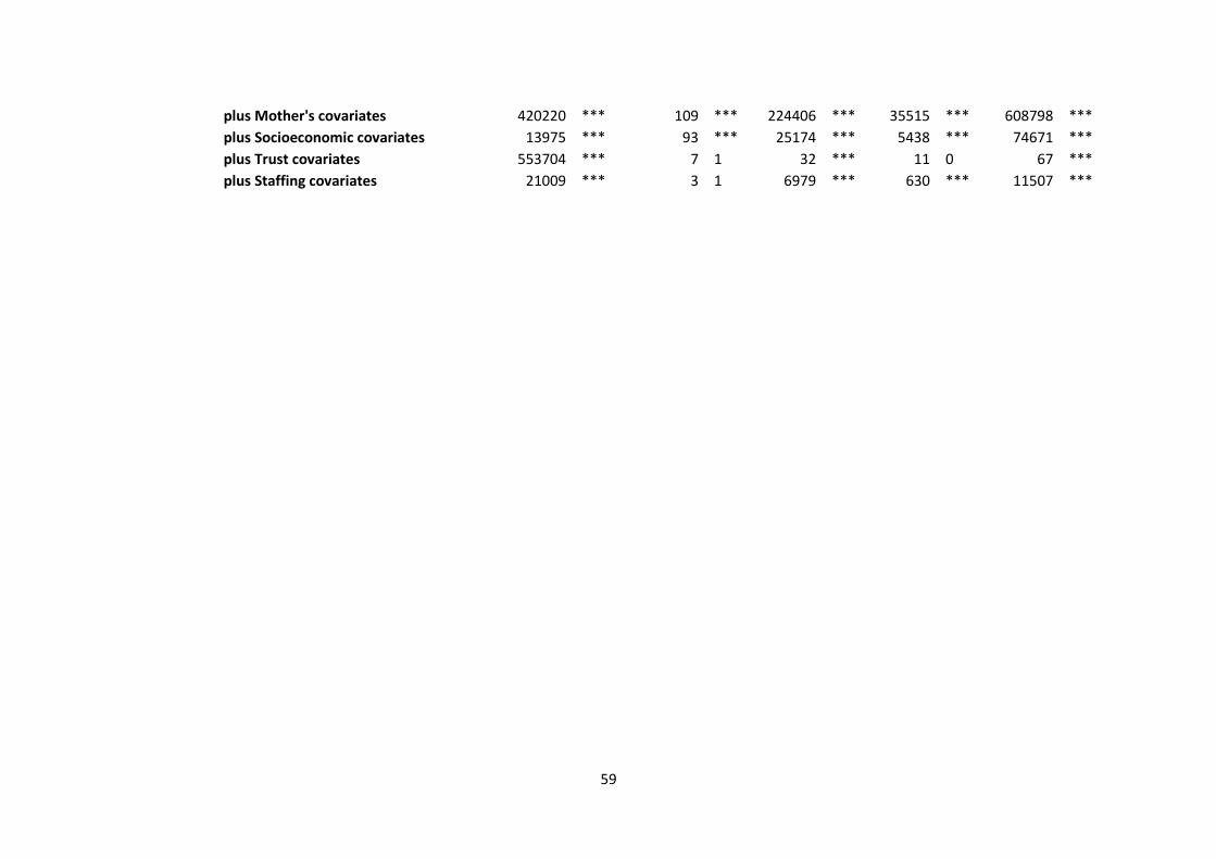
59

plus Mother's covariates 420220 *** 109 *** 224406 *** 35515 *** 608798 ***

plus Socioeconomic covariates 13975 *** 93 *** 25174 *** 5438 *** 74671 ***

plus Trust covariates 553704 *** 7 1 32 *** 11 0 67 ***

plus Staffing covariates 21009 *** 3 1 6979 *** 630 *** 11507 ***

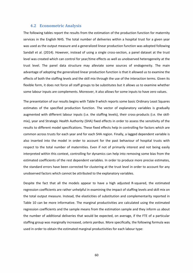
60

4.2 Econometric Analysis

The following tables report the results from the estimation of the production function for maternity

services in the English NHS. The total number of deliveries within a hospital trust for a given year

was used as the output measure and a generalized linear production function was adopted following

Sandall et al. (2014). However, instead of using a single cross-section, a panel dataset at the trust

level was created which can control for year/time effects as well as unobserved heterogeneity at the

trust level. The panel data structure may alleviate some sources of endogeneity. The main

advantage of adopting the generalized linear production function is that it allowed us to examine the

effects of both the staffing levels and the skill mix through the use of the interaction terms. Given its

flexible form, it does not force all staff groups to be substitutes but it allows us to examine whether

some labour inputs are complements. Moreover, it also allows for some inputs to have zero values.

The presentation of our results begins with Table 9 which reports some basic Ordinary Least Squares

estimates of the specified production function. The vector of explanatory variables is gradually

augmented with different labour inputs (i.e. the staffing levels), their cross-products (i.e. the skill-

mix), year and Strategic Health Authority (SHA) fixed effects in order to assess the sensitivity of the

results to different model specifications. These fixed effects help in controlling for factors which are

common across trusts for each year and for each SHA region. Finally, a lagged dependent variable is

also inserted into the model in order to account for the past behaviour of hospital trusts with

respect to the total number of maternities. Even if not of primarily interest and not being easily

interpreted within this context, controlling for dynamics can help into removing some bias from the

estimated coefficients of the rest dependent variables. In order to produce more precise estimates,

the standard errors have been corrected for clustering at the trust level in order to account for any

unobserved factors which cannot be attributed to the explanatory variables.

Despite the fact that all the models appear to have a high adjusted R-squared, the estimated

regression coefficients are rather unhelpful in examining the impact of staffing levels and skill mix on

the total output measure. Instead, the elasticities of substitution and complementarity reported in

Table 10 can be more informative. The marginal productivities are calculated using the estimated

regression coefficients and the sample means from the estimation sample and they inform us about

the number of additional deliveries that would be expected, on average, if the FTE of a particular

staffing group was marginally increased, ceteris paribus. More specifically, the following formula was

used in order to obtain the estimated marginal productivities for each labour type:

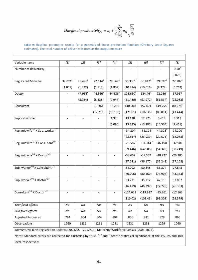
61

𝑀𝑎𝑟𝑔𝑖𝑛𝑎𝑙 𝑝𝑟𝑜𝑑𝑢𝑐𝑡𝑖𝑣𝑖𝑡𝑦𝑖 = 𝑎𝑖 +1

2∑ 𝑎𝑖𝑗

𝐾

𝑗=2

√𝑋𝑗

𝑋𝑖

Table 9: Baseline parameter results for a generalized linear production function (Ordinary Least Squares estimates). The total number of deliveries is used as the output measure

Variable name [1] [2] [3] [4] [5] [6] [7] [8]

Number of deliveriest-1 - - - - - - - .550a

(.073)

Registered Midwife 32.024a

(1.059)

23.490a

(1.432)

22.614a

(1.817)

22.562a

(1.809)

36.336a

(10.884)

36.842a

(10.616)

39.592a

(8.378)

22.707a

(6.762)

Doctor - 47.933a

(8.034)

44.326a

(8.138)

44.636a

(7.947)

128.650b

(51.480)

124.46b

(51.972)

92.266c

(51.534)

37.917

(25.083)

Consultant - - 19.364

(17.715)

18.266

(18.168)

140.200

(121.01)

152.671

(107.35)

149.755c

(83.011)

80.578c

(43.444)

Support worker - - - 1.976

(5.090)

13.128

(13.225)

12.775

(13.283)

5.618

(14.564)

3.313

(7.451)

Reg. midwife1/2

X Sup. worker1/2

- - - - -34.804

(23.637)

-34.194

(23.939)

-44.325b

(22.573)

-24.200b

(12.068)

Reg. midwife1/2

X Consultant1/2

- - - - -25.587

(69.446)

-31.314

(64.985)

-46.190

(54.328)

-37.901

(30.249)

Reg. midwife1/2

X Doctor1/2

- - - - -38.607

(37.081)

-37.507

(36.177)

-28.227

(31.241)

-20.305

(17.168)

Sup. worker1/2

X Consultant1/2

- - - - 54.702

(80.206)

50.345

(80.160)

86.374

(73.906)

27.848

(43.353)

Sup. worker1/2

X Doctor1/2

- - - - 33.271

(46.479)

35.712

(46.397)

47.116

(27.229)

37.857

(26.383)

Consultant1/2

X Doctor1/2

- - - - -124.621

(110.02)

-119.937

(109.43)

-95.861

(93.309)

-17.163

(59.379)

Year fixed effects No No No No No Yes Yes Yes

SHA fixed effects No No No No No No Yes Yes

Adjusted R-squared .784 .804 .804 .804 .806 .811 .828 .865

Observations 1260 1231 1231 1231 1231 1231 1229 1060

Source: ONS Birth registration Records (2004/05 – 2012/13); Maternity Workforce Census (2004-2014).

Notes: Standard errors are corrected for clustering by trust. a,

b and

c denote statistical significance at the 1%, 5% and 10%

level, respectively.

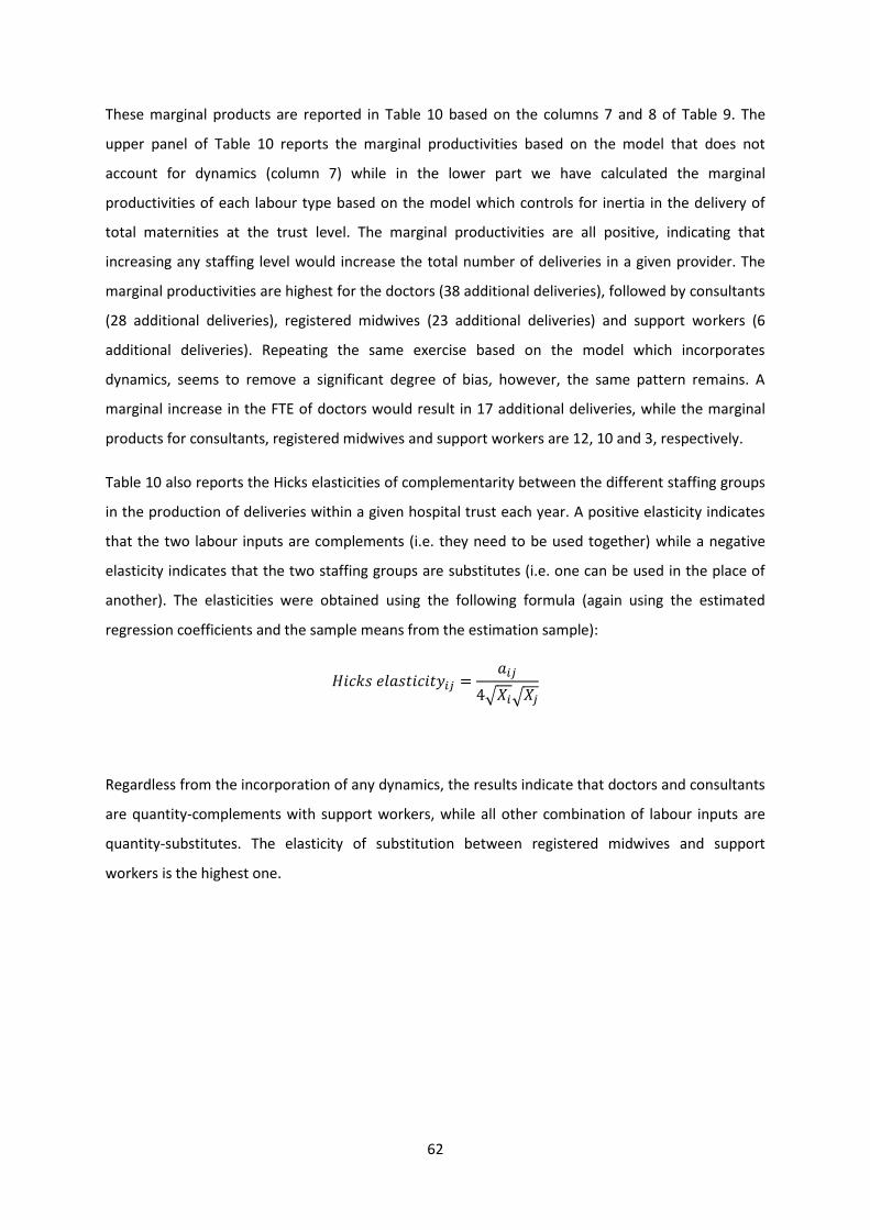
62

These marginal products are reported in Table 10 based on the columns 7 and 8 of Table 9. The

upper panel of Table 10 reports the marginal productivities based on the model that does not

account for dynamics (column 7) while in the lower part we have calculated the marginal

productivities of each labour type based on the model which controls for inertia in the delivery of

total maternities at the trust level. The marginal productivities are all positive, indicating that

increasing any staffing level would increase the total number of deliveries in a given provider. The

marginal productivities are highest for the doctors (38 additional deliveries), followed by consultants

(28 additional deliveries), registered midwives (23 additional deliveries) and support workers (6

additional deliveries). Repeating the same exercise based on the model which incorporates

dynamics, seems to remove a significant degree of bias, however, the same pattern remains. A

marginal increase in the FTE of doctors would result in 17 additional deliveries, while the marginal

products for consultants, registered midwives and support workers are 12, 10 and 3, respectively.

Table 10 also reports the Hicks elasticities of complementarity between the different staffing groups

in the production of deliveries within a given hospital trust each year. A positive elasticity indicates

that the two labour inputs are complements (i.e. they need to be used together) while a negative

elasticity indicates that the two staffing groups are substitutes (i.e. one can be used in the place of

another). The elasticities were obtained using the following formula (again using the estimated

regression coefficients and the sample means from the estimation sample):

𝐻𝑖𝑐𝑘𝑠 𝑒𝑙𝑎𝑠𝑡𝑖𝑐𝑖𝑡𝑦𝑖𝑗 =𝑎𝑖𝑗

4√𝑋𝑖√𝑋𝑗

Regardless from the incorporation of any dynamics, the results indicate that doctors and consultants

are quantity-complements with support workers, while all other combination of labour inputs are

quantity-substitutes. The elasticity of substitution between registered midwives and support

workers is the highest one.

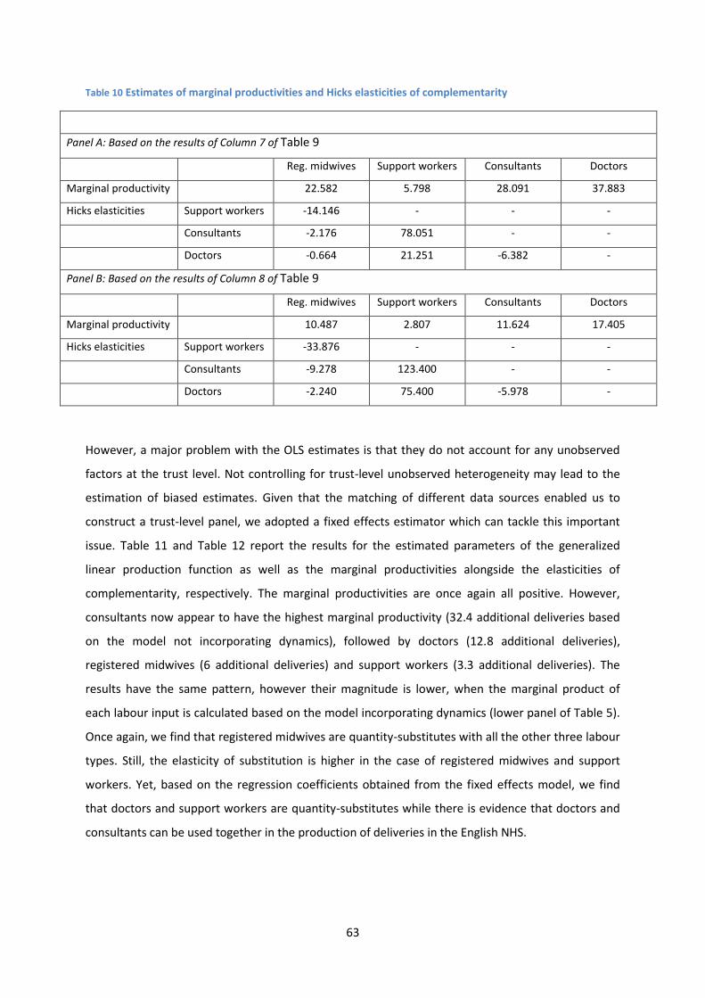
63

Table 10 Estimates of marginal productivities and Hicks elasticities of complementarity

Panel A: Based on the results of Column 7 of Table 9

Reg. midwives Support workers Consultants Doctors

Marginal productivity 22.582 5.798 28.091 37.883

Hicks elasticities Support workers -14.146 - - -

Consultants -2.176 78.051 - -

Doctors -0.664 21.251 -6.382 -

Panel B: Based on the results of Column 8 of Table 9

Reg. midwives Support workers Consultants Doctors

Marginal productivity 10.487 2.807 11.624 17.405

Hicks elasticities Support workers -33.876 - - -

Consultants -9.278 123.400 - -

Doctors -2.240 75.400 -5.978 -

However, a major problem with the OLS estimates is that they do not account for any unobserved

factors at the trust level. Not controlling for trust-level unobserved heterogeneity may lead to the

estimation of biased estimates. Given that the matching of different data sources enabled us to

construct a trust-level panel, we adopted a fixed effects estimator which can tackle this important

issue. Table 11 and Table 12 report the results for the estimated parameters of the generalized

linear production function as well as the marginal productivities alongside the elasticities of

complementarity, respectively. The marginal productivities are once again all positive. However,

consultants now appear to have the highest marginal productivity (32.4 additional deliveries based

on the model not incorporating dynamics), followed by doctors (12.8 additional deliveries),

registered midwives (6 additional deliveries) and support workers (3.3 additional deliveries). The

results have the same pattern, however their magnitude is lower, when the marginal product of

each labour input is calculated based on the model incorporating dynamics (lower panel of Table 5).

Once again, we find that registered midwives are quantity-substitutes with all the other three labour

types. Still, the elasticity of substitution is higher in the case of registered midwives and support

workers. Yet, based on the regression coefficients obtained from the fixed effects model, we find

that doctors and support workers are quantity-substitutes while there is evidence that doctors and

consultants can be used together in the production of deliveries in the English NHS.

64

Table 11: Baseline parameter results for a generalized linear production function (Fixed Effects estimates). The total number of deliveries is used as the output measure

Variable name [1] [2] [3] [4] [5] [6] [7] [8]

Number of deliveriest-1 - - - - - - - .0229

(.063)

Registered Midwife 10.117a

(2.512)

8.735a

(2.510)

6.771b

(2.826)

6.662b

(2.879)

25.016a

(14.206)

25.520c

(14.437)

25.506c

(14.445)

23.077a

(15.574)

Doctor - 22.835a

(5.346)

19.007a

(5.197)

18.701a

(5.168)

54.364a

(20.641)

39.322c

(20.615)

39.459c

(20.705)

35.211c

(23.821)

Consultant - - 43.959b

(18.298)

42.805b

(18.250)

40.875

(118.93)

4.675

(134.62)

4.479

(134.69)

-10.111

(155.80)

Support worker - - - 3.912

(5.001)

3.501

(10.199)

0.437

(10.078)

0.433

(10.077)

-2.719

(13.448)

Reg. midwife1/2

X Sup. worker1/2

- - - - -19.056

(16.215)

-15.641

(15.357)

-15.658

(15.360)

-14.404

(18.784)

Reg. midwife1/2

X Consultant1/2

- - - - -43.532

(70.633)

-49.509

(76.272)

-49.342

(76.357)

-41.206

(87.516)

Reg. midwife1/2

X Doctor1/2

- - - - -51.528b

(26.043)

-51.507c

(29.374)

-51.776c

(29.378)

-51.756

(32.867)

Sup. worker1/2

X Consultant1/2

- - - - 86.123

(55.858)

82.984

(54.855)

83.054

(54.872)

63.461

(63.938)

Sup. worker1/2

X Doctor1/2

- - - - -11.760

(24.149)

-15.980

(24.213)

-15.982

(24.210)

-2.200

(29.068)

Consultant1/2

X Doctor1/2

- - - - 82.253

(90.206)

114.739

(91.720)

114.543

(91.802)

115.263

(101.92)

Year fixed effects No No No No No Yes Yes Yes

SHA fixed effects No No No No No No Yes Yes

Adjusted R-squared .060 .083 .093 .093 .100 .154 .153 .091

Observations 1260 1231 1231 1231 1231 1231 1229 1061

Source: ONS Birth registration Records (2004/05 – 2012/13); Maternity Workforce Census (2004-2014).

Notes: Standard errors are corrected for clustering by trust. a,

b and

c denote statistical significance at the 1%, 5% and 10%

level, respectively.

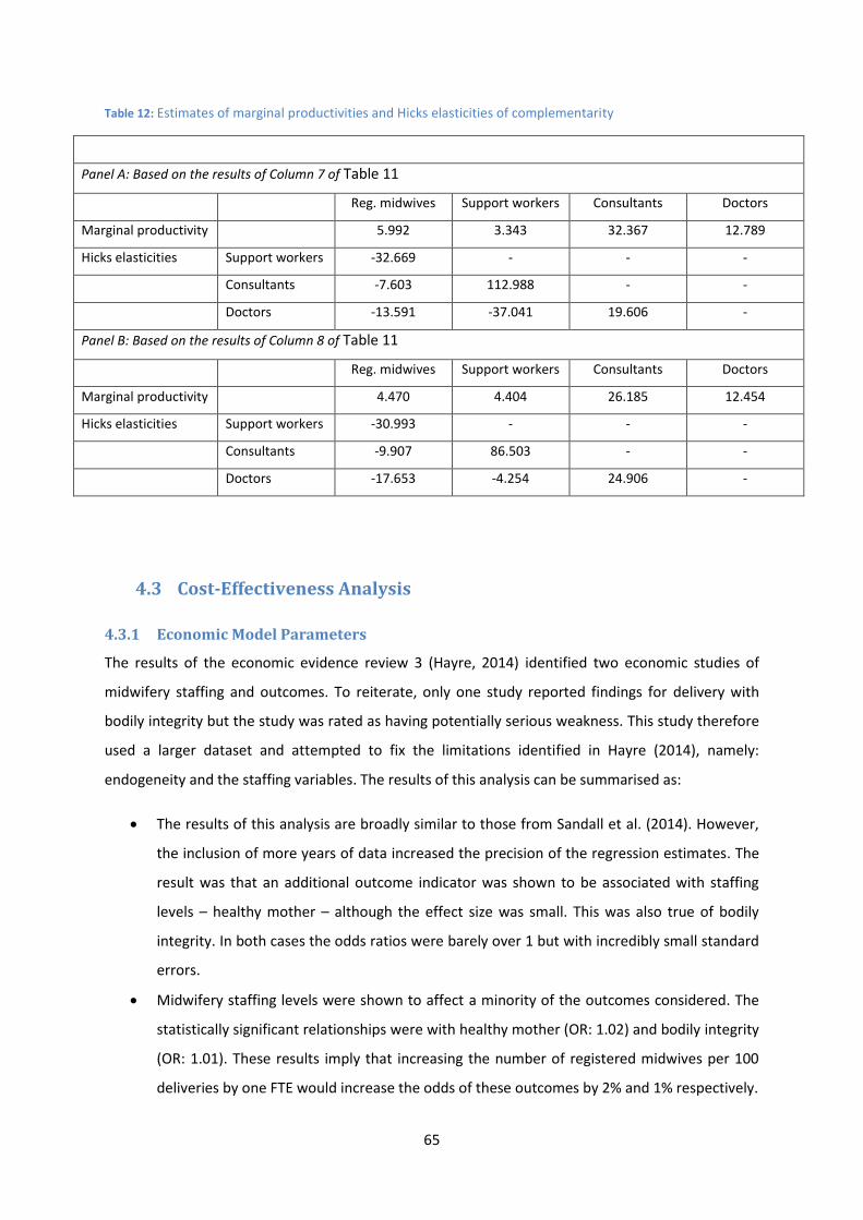
65

Table 12: Estimates of marginal productivities and Hicks elasticities of complementarity

Panel A: Based on the results of Column 7 of Table 11

Reg. midwives Support workers Consultants Doctors

Marginal productivity 5.992 3.343 32.367 12.789

Hicks elasticities Support workers -32.669 - - -

Consultants -7.603 112.988 - -

Doctors -13.591 -37.041 19.606 -

Panel B: Based on the results of Column 8 of Table 11

Reg. midwives Support workers Consultants Doctors

Marginal productivity 4.470 4.404 26.185 12.454

Hicks elasticities Support workers -30.993 - - -

Consultants -9.907 86.503 - -

Doctors -17.653 -4.254 24.906 -

4.3 Cost-Effectiveness Analysis

4.3.1 Economic Model Parameters

The results of the economic evidence review 3 (Hayre, 2014) identified two economic studies of

midwifery staffing and outcomes. To reiterate, only one study reported findings for delivery with

bodily integrity but the study was rated as having potentially serious weakness. This study therefore

used a larger dataset and attempted to fix the limitations identified in Hayre (2014), namely:

endogeneity and the staffing variables. The results of this analysis can be summarised as:

The results of this analysis are broadly similar to those from Sandall et al. (2014). However,

the inclusion of more years of data increased the precision of the regression estimates. The

result was that an additional outcome indicator was shown to be associated with staffing

levels – healthy mother – although the effect size was small. This was also true of bodily

integrity. In both cases the odds ratios were barely over 1 but with incredibly small standard

errors.

Midwifery staffing levels were shown to affect a minority of the outcomes considered. The

statistically significant relationships were with healthy mother (OR: 1.02) and bodily integrity

(OR: 1.01). These results imply that increasing the number of registered midwives per 100

deliveries by one FTE would increase the odds of these outcomes by 2% and 1% respectively.

66

There was no statistically significant relationship between any of the staffing groups and

maternal mortality, stillborn of healthy baby so these outcomes were not considered

further.

Besides reducing the uncertainty of the parameter estimates, the use of longitudinal data in

this study has also allowed for the control of time invariant unobserved heterogeneity which

may have confounded earlier studies. This combined with the inclusion of a patient level risk

measure should reduce the risk of omitted variable bias but it is impossible to guarantee

this. Attempts to econometrically solve the problem were unsuccessful.

The addition of the Hospital Load Variable provided inconsistent results. Worsening staff to

patient ratios had a strong and statistically significant effect on the healthy mother outcome,

but had positive but weak and marginally significant effects on both the healthy baby and

bodily integrity. There is no practical interpretation of the odds ratio. These contradictory

findings are confusing but indicate that further work around improving the measurement of

the staffing variables may be fruitful.

Table 13 presents the parameter values that will be used as the base case for the analysis alongside

the upper and lower values to be used in the sensitivity analysis, which are derived from the

descriptive and inferential statistical analysis reported in Section 4. The lower and upper values are

based upon a plausible range of values.

For staff costs, the lower value is set to the bottom of the relevant Agenda for Change band (e.g.

Band 5) discounted by the out of London factor of 0.96, and for the upper value the top of the

relevant Agenda for Change band (e.g. band 6) is used, multiplied by the London weighting factor

used by PSSRU of 1.19. In both cases the employer’s on-costs (14% pension contributions and 13.8%

national insurance contributions above £146 per week) are included to make this comparable to the

national mean wages reported by PSSRU (Curtis, 2013). This provides an average cost of £39,640 for

per additional midwife, with a range of £25,400 to £51,413. The base case level of staffing was set at

the average number of midwives per 100 deliveries in 2013, which was 3.34. The minimum staffing

ratio that year was 1.55 and the maximum 16.71. These values are highly unlikely but provide a good

test of the sensitivity of the model to the underlying assumptions.

The number of expected cases of, for example, healthy mother in the average trust is determined by

their rate and the number of deliveries. The base case number of deliveries (4,620) is set at the

sample mean for the most recent year of data (2013), and the upper (10,680) and lower values

(1,210) are set at the maximum and minimum values. Similarly, the current (before intervention)

rate of occurrence is set at the 2013 sample average for the base case and the minimum and

67

maximum values for the lower and upper values of the sensitivity analysis. For example for bodily

integrity that would be an average trust rate of 30% in 2013 with a range of 15% to 45%.

Due to the nature of the odds ratio that is calculated from a logistic regression, the most natural

intervention to consider is increasing the staffing variable by one unit at a time. That corresponds to

1 FTE midwife per 100 deliveries, and for the average trust that is equivalent to increasing the

midwifery workforce by 46 FTE or roughly 33%: a substantial intervention. Against this a lower

bound of 0.5 units and an upper bound of 2 were chosen for comparison.

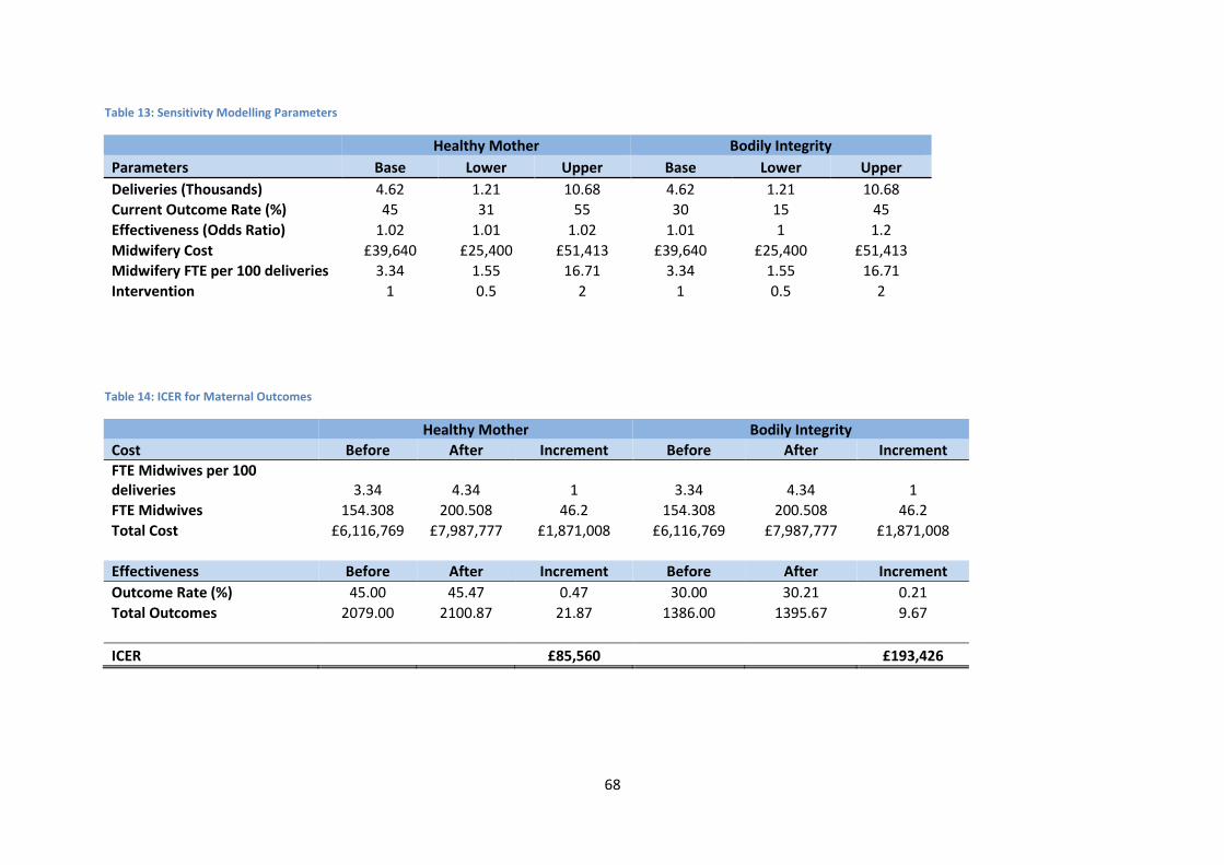
68

Table 13: Sensitivity Modelling Parameters

Healthy Mother Bodily Integrity

Parameters Base Lower Upper Base Lower Upper

Deliveries (Thousands) 4.62 1.21 10.68 4.62 1.21 10.68

Current Outcome Rate (%) 45 31 55 30 15 45

Effectiveness (Odds Ratio) 1.02 1.01 1.02 1.01 1 1.2

Midwifery Cost £39,640 £25,400 £51,413 £39,640 £25,400 £51,413

Midwifery FTE per 100 deliveries 3.34 1.55 16.71 3.34 1.55 16.71

Intervention 1 0.5 2 1 0.5 2

Table 14: ICER for Maternal Outcomes

Healthy Mother Bodily Integrity

Cost Before After Increment Before After Increment

FTE Midwives per 100 deliveries 3.34 4.34 1 3.34 4.34 1

FTE Midwives 154.308 200.508 46.2 154.308 200.508 46.2

Total Cost £6,116,769 £7,987,777 £1,871,008 £6,116,769 £7,987,777 £1,871,008

Effectiveness Before After Increment Before After Increment

Outcome Rate (%) 45.00 45.47 0.47 30.00 30.21 0.21

Total Outcomes 2079.00 2100.87 21.87 1386.00 1395.67 9.67

ICER £85,560 £193,426

69

4.3.2 Cost-Effectiveness

The incremental cost of increasing the number of midwives by 1 FTE per 100 deliveries is the same

irrespective of the outcome under consideration. The incremental cost is £1.8 million for the

average trust as Table 14 illustrates. This represents an approximate expansion of the midwifery

workforce of a third, whilst the statistical analysis predicted an improvement in the outcomes of 1-

2% in the odds.

The Incremental Cost Effectiveness Ratios (ICERs) are therefore £85,560 per healthy mother and

£193,426 per mother with bodily integrity. This is in comparison to current practice i.e. the current

level of staffing and skill mix. ICERs were not calculated for the remaining outcomes as there is no

evidence that they are effective at present.

As we cannot express this ICER in a universal ‘currency’ such as QALYs, it is difficult to establish

whether this represents value for money: whether it generates more health benefit than another

intervention it may displace. However, taking a broad threshold of cost-effectiveness of £20-30,000

per QALY then a ‘healthy mother’ would need to generate 2.9-4.3 QALYs to be in the borderline

region and over 4.3 to be cost-effective. Similarly, each mother with bodily integrity would need to

generate QALYs equivalent to 6.4-9.7.

However this underestimates the cost-effectiveness in a number of ways. First, it hasn't been

possible to net off the NHS savings from the intervention e.g. reduced overnight stays associated

with a healthy mother. Second, one intervention (increasing the number of midwives by 1 FTE per

100 deliveries) generates both positive outcomes and they need to be combined some how to give a

fairer representation of the true cost-effectiveness. In the absence of a common metric this is not

possible.

4.3.3 Sensitivity Analysis

A one-way sensitivity analysis was performed whereby each of the parameters in Table 13 were

varied from the base case to their upper and lower values. The sensitivity analysis demonstrates to

what extent the results of the CEA are influenced by the assumptions that have been made, and

allow the uncertainty in the parameter values to be illustrated. Table 15 presents the results of the

sensitivity analysis for the ICER for all outcomes.

As there is an assumption that the effect of increasing staffing levels on the outcome is constant

across all levels of the staffing variable then altering the assumptions around the size of the

70

intervention, the current level of staffing or the number of deliveries per trust does not alter the

ICERs. The assumptions that alter the ICER are the cost of staffing (cost), the effect of staffing on the

outcomes in question (effectiveness) and the current level of the outcome (baseline).

If the assumption is that all midwives regardless of grade ‘produce’ the same effect on the

outcomes, ceteris paribus, then it is fairly obvious that employing lower grade and therefore

cheaper staff as part of the intervention will be more cost-effective. This report has not considered

the impact on the supply of midwives of an introduction of the proposed intervention across all

providers simultaneously. There are unanswered questions surrounding the availability of additional

midwives (especially at the lower grades) and the effect on market conditions of an increase in

demand for midwives.

It is clear that the effectiveness is the most important assumption with respect to the cost-

effectiveness of the intervention. For example, as the odds ratio on bodily integrity is weak (1.01)

this assumption is both fragile and important. A small change in this assumption can have dramatic

effects on the ICER as Table 15 clearly illustrates.

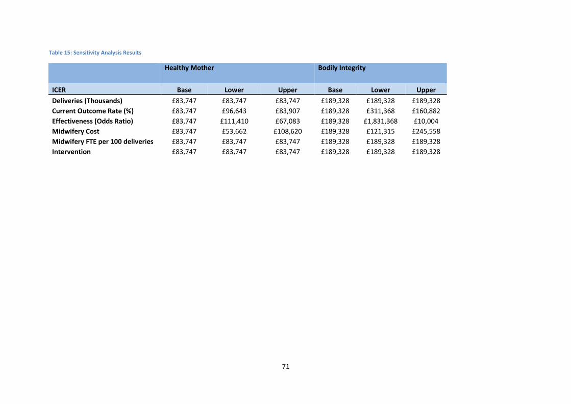
71

Table 15: Sensitivity Analysis Results

Healthy Mother Bodily Integrity

ICER Base Lower Upper Base Lower Upper

Deliveries (Thousands) £83,747 £83,747 £83,747 £189,328 £189,328 £189,328

Current Outcome Rate (%) £83,747 £96,643 £83,907 £189,328 £311,368 £160,882

Effectiveness (Odds Ratio) £83,747 £111,410 £67,083 £189,328 £1,831,368 £10,004

Midwifery Cost £83,747 £53,662 £108,620 £189,328 £121,315 £245,558

Midwifery FTE per 100 deliveries £83,747 £83,747 £83,747 £189,328 £189,328 £189,328

Intervention £83,747 £83,747 £83,747 £189,328 £189,328 £189,328

72

5 Discussion

Generally, staffing levels (per 100 deliveries) were not related to the outcomes under consideration.

The exception was midwifery staffing levels (per 100 deliveries), which were associated with the

healthy mother (OR: 1.02) and bodily integrity (OR: 1.01) outcomes. However, these relationships

were weak; the odds ratios imply that increasing the number of registered midwives per 100

deliveries by one FTE would increase the odds of these outcomes by 2% and 1% respectively.

Based upon these measures of effectiveness Incremental Cost Effectiveness Ratios were estimated:

£85,560 per healthy mother and £193,426 per mother with bodily integrity. This is in comparison to

current practice i.e. the current level of staffing and skill mix. ICERs were not calculated for the

remaining outcomes as there was no evidence that they were effective at present.

The econometric modelling attempted to model the effect of skill mix on hospital production. It did

not consider the outcomes. The results were very similar with or without the inclusion of dynamic

effects which indicates that endogeneity is not biasing the results. The econometric results indicate

that doctors and consultants are quantity-complements with support workers, while all other

combination of labour inputs are quantity-substitutes.

The data and results are consistent with the extant literature. For instance comparing the descriptive

statistics produced from the HES data in Table 6 with those reported in Sandall et al. (2014), they are

broadly similar despite the current analysis expanding the dataset from one to ten years. Similarly to

the HES patient level data, there is a strong correlation between the trust level data (e.g. staffing)

and those reported in Sandall et al. (2014). For instance, the 2010 FTE midwives per 100 deliveries is

3.10 in this study and 3.08 in Sandall et al. (2014).

5.1 Statistical Analysis Limitations

The outcome analyses presented here have the limitation present in all observational studies in that

they do not test causal associations. We are therefore unable to conclude that alteration of staffing

skill mix or any of the other predictor variables will have a beneficial (or detrimental) impact on

patient outcomes. A cluster-randomised controlled trial may be required to identify causal

associations and the impact of staffing changes. Finally, there may be an endogeneity problem in

that trusts with better patient outcomes may also have higher levels of staffing or richer skill mixes

for another reason (e.g. high quality management) which is excluded from the models. Some of the

potential causes of omitted variable bias have been removed through the use of longitudinal data, to

the extent to which these factors are fixed over time. Early attempts have been made to tackle the

73

potential endogeneity problem through econometric means but further research with more time

could make more headway. This was only possible with the econometric models which tackled the

issue of skill mix and staffing levels on the number of deliveries. It was not possible to make similar

progress with the statistical modelling of the outcomes.

Secondary data analysis is always dependent upon the quality of the data. A full census of women’ s

deliveries from HES (2003-2013) was used so there was no bias caused by non-response. Instead,

biases could be caused by missing data, poorly coded data or omitted variables from the clinical risk

model. Extensive data cleaning was conducted to remove duplicate records and records which did

not relate to a delivery episode. Trusts were excluded where fewer than 80% of women could be

coded for a particular indicator, which limited the dataset for some potential indicators.

A problem when using routinely collected data is that analysis is limited to variables that are

(reliably) collected. For example, body mass index and smoking or drug use were excluded from the

models because of data quality issues, although they are known to be important risk factors. Only a

limited set of trust-level variables were used. Organisational variables (e.g. organisational climate),

service configuration (e.g. Obstetric led unit) and models of care that could be important predictors

were not available. The models may also have omitted other variables, either known or unknown,

that are predictive of outcome.

Staffing data were available only at trust level so we could not explore the effects of staffing at the

unit level. The data for trusts that have multiple units could not be disaggregated. Aggregated trust-

level data makes the assumption that unit-level effects within a trust are similar, which may not be

true. The staffing data are taken from a census undertaken every September. This single-point

estimate will hide any fluctuations that may occur over time. We analysed data that were

aggregated over a period of a year. These data will therefore miss those occasions when the service

is placed under stress, or reaching a critical point, because of excess deliveries, low staffing levels or

other factors. Further it was not possible to divide the staffing numbers between obstetric and

gynaecology services.

An attempt was made to create variation in staffing levels by creating a new Hospital Load Ratio

variable. This divided the approximate number of deliveries each day by the total staffing numbers

to create variation in staffing driven by changes in service demand. As not all staff will be working on

any particular day on the delivery ward this is a particularly crude proxy. Despite this, the variable

provided some important insights being a statistically significant predictor of the outcomes. This is

significant improvement over existing studies. However, interpreting the coefficient on this variable

for practical purposes is impossible. Instead it underlines the importance of collecting better ward

74

level staffing data on a daily or shift basis, as well as being able to link these back to patient’s and

therefore their outcomes.

Finally, whilst the significantly larger dataset used here made previously insignificant relationships

statistically significant, the effect sizes were marginal. A large change (circa a third of the workforce)

would be required to generate a very small change in the outcome (typically 10-20 cases per

annum).

5.2 Cost-Effectiveness Analysis limitations

The economic evaluation was stymied by the lack of clear evidence on the effectiveness of the

intervention i.e. on the relationship between staffing levels, skill mix and outcomes in maternity

services. The limitations described in the previous section indicate that the current statistical

analysis is imperfect. However, it is a significant improvement over the existing evidence base and

short of an experiment (natural, quasi, or real) it is difficult to imagine how better evidence could be

assembled. As a result, a cost-effectiveness analysis could only be performed for healthy mother and

bodily integrity.

No universal outcome measure (e.g. QALY) was available to aggregate all of the possible benefits of

altering staffing levels. When calculating the cost-effectiveness of the interventions other potential

effects have been omitted. Thus, while it is uncertain, the estimate of the cost-effectiveness could

be an underestimate of the true benefit of increasing nurse staffing or skill mix changes.

As a result of poor staffing variables that do not adequately measure the true patient-staff ratio and

its variation over time and provider, the resulting statistical findings were marginal. This study found

more of the outcomes to be statistically significantly related to staffing but this was driven by the

size of the dataset which improves the precision of the estimates. However, the effect sizes like in

previous studies are practically very small. The findings of this study are therefore congruent with

the extant evidence.

5.3 Recommendations for Future Research

There are three main areas for future research. First, improving the collection of ward level staffing

data that could be linked to patients and their outcomes is important. A major weakness of this and

existing research is the aggregate nature of the staffing data. The progress made through the

inclusion of the Hospital Load Ratio demonstrates that this would be a fruitful avenue of research.

75

Second, designing the implementation of a Maternity Safe Staffing guideline or other staffing

intervention in such a way as to create a quasi or natural experiment would be invaluable. At

present there is no casual link between staffing and outcomes and the best available evidence does

not support a strong relationship between these variables. An experimental design would enable

researchers to answer the question conclusively but randomising the numerous omitted variables.

Finally, in the absence of an experimental research design more work could be done to find

econometric solutions to the endogeneity problem. Early steps were taken in this study to address

the issue but time constraints limited the progress that could be made. Future research could adopt

the approach used in this study (generalized methods of moments to exploit the time dimension in

the data) or careful consideration could be given to instruments for the staffing variables that would

remove any potential endogeneity. A good instrument would need to be strongly correlated with

the staffing variable of interest (e.g. midwife numbers) but uncorrelated with the outcome directly.

5.4 Evidence Summary

This report complements the systematic Evidence Reviews [1-3] produced by Bazian Ltd and NICE,

and aimed to produce a cost-effectiveness analysis of increasing midwife staffing levels on five

maternity outcomes: maternal and infant mortality, healthy mother and baby and bodily integrity.

The evidence contained in this report can be summarised as follows:

Due to a lack of published applicable studies, the relationship between midwifery staffing

levels and a range of outcomes were analysed using HES data from English NHS trusts 2003-

2014.

The results were largely consistent with the existing evidence, although this work corrected

a number of issues with the extant literature.

Midwifery staffing levels were shown to affect a minority of the outcomes considered. The

statistically significant relationships were with healthy mother (OR: 1.02) and bodily integrity

(OR: 1.01). These results imply that increasing the number of registered midwives per 100

deliveries by one FTE would increase the odds of these outcomes by 2% and 1% respectively.

There was no statistically significant relationship between any of the staffing groups and

maternal mortality, stillborn of healthy baby so these outcomes were not considered

further.

Based upon these measures of effectiveness Incremental Cost Effectiveness Ratios were

estimated as £85,560 per healthy mother and £193,426 per mother with bodily integrity.

76

Decision making in the absence of a universal measure, such as QALYS, is difficult but if the

outcomes were each generating 2-3 QALYs they could be considered cost-effective. This is

not currently known. Ultimately, the cost-effectiveness will depend upon the NHS’s

willingness to pay for these particular outcomes.

The econometric results indicate that doctors and consultants are quantity-complements

with support workers, while all other combination of labour inputs are quantity-substitutes.

The elasticity of substitution between registered midwives and support workers is the

highest one. All marginal productivities are positive. The econometric findings were robust

to the inclusion of dynamic effects.

Most variation in the outcomes was accounted for at the individual, patient level (within

trust level) rather than between trusts. Regression models explain the variation in the

outcome variable by the variation in the explanatory variables. As the staffing variables did

not vary within trusts they were unable to explain much of the variation in the outcomes.

The addition of the Hospital Load Variable provided inconsistent results. Worsening staff to

patient ratios had a strong and statistically significant effect on the healthy mother outcome,

but had positive but weak and marginally significant effects on both the healthy baby and

bodily integrity.

The last two points indicate that further works needs to be done on collecting unit level data

that varies over time (e.g shift by shift), especially where this can be matched to patient

demand data.

Patient level factors are clearly very important, with age, ethnicity and parity being

associated with both outcomes and deprivation also being associated with bodily integrity.

In both cases, the largest odds ratio is for the clinical risk variable. A mother classed as

“higher risk” is half as likely to deliver with bodily integrity than a mother classed as “lower

risk”.

There is a clear time dimension to the results, with each year being strongly significantly

related to the outcome. When compared to 2004 (the base year) each year since has a lower

rate of healthy mothers and bodily integrity. This was also clear in the descriptive statistics in

Section 4.1.1.

In terms of the trust level variables, larger trusts have lower healthy mother rates but this

effect is weak.

This is the largest study on this topic to date. The use of longitudinal data combined with

the inclusion of a patient level risk measure should reduce the risk of omitted variable bias

77

but it is impossible to guarantee this. Attempts to econometrically solve the problem were

largely unsuccessful.

Trusts should be encouraged to monitor both planned and actual staffing levels at ward level

and to match these to outcomes of care. The adoption of Safe Staffing tools that include the

monitoring of staffing and patient acuity data should be welcomed.

Future research should concentrate on (i) improving the collection of staffing data to allow

for within trust variation in staffing, (ii) tackling the inherent problem of endogeneity most

likely through innovative research designs, and (iii) measuring the utility of the outcomes to

enable the calculation of QALYs and the aggregation of the outcomes into a single measure.

78

6 References

Allen M, and Thornton S (2013) Providing one-to-one care in labour. Analysis of 'Birthrate Plus'

labour ward staffing in real and simulated labour ward environments BJOG: An International Journal

of Obstetrics & Gynaecology, 120 (1): 100-107

Allison, P. (1984). Event history analysis. Newbury Park, CA: Sage Publications.

Association of University Hospital Trusts (2014) List of AUKUH Members. URL:

http://www.aukuh.org.uk/index.php/members/aukuh-members

(Accessed 10 November 2014)

Bazian Ltd (2014) Evidence review 1: An evidence review on the association between midwifery

staffing at a local level and maternal and neonatal outcomes, and factors affecting these

requirements, Report for NICE Safe Staffing Advisory Committee, July 2014, Bazian Ltd, London: UK.

Berndt E, and Christensen L. (1973) The Translog Function and the Substitution of Equipment,

Structures and Labour in U.S. Manufacturing, Journal of Econometrics, 1 (1): 81–114.

CMACE (2011) Saving Mothers' Lives. Reviewing maternal deaths to make motherhood safer: 2006-

2008; Centre for Maternal and Child Enquiries (CMACE), BJOG: An International Journal of Obstetrics

& Gynaecology, 118(1): Supplement

Curtis, L. (2013) [Ed.] Unit Costs for Health and Social Care 2013, Personal Social Services Research

Unit, Canterbury: UK

DCLG (2011) The English Indices of Deprivation 2010, Neighbourhood Statistics Release . 2011. URL:

http://webarchive.nationalarchives.gov.uk/20120919132719/http://www.communities.gov.uk/docu

ments/statistics/pdf/1871208.pdf

(Accessed 10 December 2014).

Diewert WE. (1971) An Application of the Shephard Duality Theorem: A Generalized Leontif

Production Function, Journal of Political Economy, 79 (3):507.

Hayre, J (2014) Evidence review 3: Economic Evidence Review in Safe Staffing for Maternity Settings,

Report for NICE Safe Staffing Advisory Committee, August 2014, NICE, London: UK.

Hicks JR. (1970) Elasticities of Substitution Again: Substitutes and Complements, Oxford Economic

Papers, 22 (3): 289–96.

79

HSCIC (2010) Hospital Episode Statistics Data Dictionary – Inpatients, NHS Health and Social Care

Information Centre. URL: http://www.hscic.gov.uk/media/1358/HES-Hospital-Episode-Statistics-HES-

Admitted-Patient-Data-Dictionary/pdf/HES_Inpatients_DD_Sept10.pdf

(Accessed 15 December 2014)

Knight HE, Gurol-Urganci I, Mahmood TA, Templeton A, Richmond D, van der Meulen JH, et al.

(2013) Evaluating maternity care using national administrative health datasets: how are statistics

affected by the quality of data on method of delivery? BMC Health Services Research, 13: 200.

Knight M, Kenyon S, Brocklehurst P, Neilson J, Shakespeare J, Kurinczuk JJ, eds [on behalf of

MBRRACE-UK] (2014) Saving lives, improving mothers’ care—lessons learned to inform future

maternity care from the UK and Ireland Confidential Enquiries into Maternal Deaths and Morbidity

2009-12. Dec 2014. http://www.npeu.ox.ac.uk/mbrrace-uk/reports

(Accessed 14 December, 2014)

Murray J, Saxena S, Modi N, Majeed A, Aylin P, Bottle A. (2012) Quality of routine hospital birth

records and the feasibility of their use for creating birth cohorts. Journal of Public Health, 35: 298–

307.

NICE (2007) Intrapartum Care: Care of Healthy Women and Their Babies During Childbirth . NICE

Clinical Guideline 55. URL: www.nice.org.uk/guidance/cg55/resources/guidance-intrapartum-

carepdf

(Accessed 10 September 2014)

Reinhardt U. (1972) A Production Function for Physician Services, Review of Economics and Statistics,

54 (1): 55–66.

Sandall J, Murrells T, Dodwell M, Gibson R, Bewley S, Coxon K, Bick D, Cookson G, Warwick C, and

Hamilton-Fairley D. (2014) The efficient use of the maternity workforce and the implications for

safety & quality in maternity care, Health Service and Delivery Research, 2 (38): October 2014

Sato R, Koizumni T (1973) On the Elasticities of Substitution and Complementarity, Oxford Economic

Papers, 25 (1): 44–56.

Syrquin M, Hollender G. (1982) Elasticities of Substitution and Complementarity: The General Case.

Oxford Economic Papers, 34 (3): 515–9.

80

7 Appendix A: Full Statistical Results

For clarity and for ease of interpretation, only a summary of the statistical findings are presented in the main report in Section 4.1.2. This Appendix contains

all of the relevant regression output.

Table 16: Healthy Mother Full Regression Results

Std. Error

Odds Ratio

Odds Ratio

Beta t-

statistic p-

value Lower

CI Upper

CI

Intercept

-0.188 0.045 0.045 0.000 0.829 0.758 0.906

Maternal Age Missing 0.183 0.021 0.021 0.000 1.201 1.153 1.251

<20 -0.476 0.006 0.006 0.000 0.621 0.614 0.629

20-24 -0.499 0.005 0.005 0.000 0.607 0.601 0.614

25-29 -0.425 0.005 0.005 0.000 0.654 0.647 0.660

30-34 -0.331 0.005 0.005 0.000 0.718 0.711 0.726

35-39 -0.205 0.005 0.005 0.000 0.815 0.807 0.824

>40 0.000

0.000

0.000

0.000

Higher Risk

1.092 0.002 0.002 0.000 2.980 2.969 2.992

Ethnicity British (White) -0.130 0.006 0.006 0.000 0.878 0.867 0.888

Irish (White) -0.003 0.015 0.015 0.839 0.997 0.969 1.026

Any other White background -0.077 0.007 0.007 0.000 0.926 0.914 0.938

White and Black Caribbean 0.006 0.015 0.015 0.678 1.006 0.976 1.037

White and Black African 0.235 0.018 0.018 0.000 1.265 1.221 1.310

White and Asian -0.050 0.020 0.020 0.013 0.951 0.914 0.990

Any other Mixed background -0.016 0.014 0.014 0.230 0.984 0.958 1.010

Indian 0.094 0.008 0.008 0.000 1.098 1.081 1.116

Pakistani 0.090 0.008 0.008 0.000 1.094 1.078 1.110

Bangladeshi 0.084 0.010 0.010 0.000 1.087 1.066 1.109

Any other Asian background 0.067 0.009 0.009 0.000 1.070 1.051 1.088

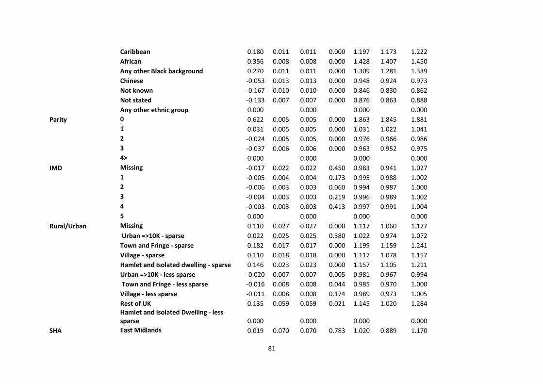
81

Caribbean 0.180 0.011 0.011 0.000 1.197 1.173 1.222

African 0.356 0.008 0.008 0.000 1.428 1.407 1.450

Any other Black background 0.270 0.011 0.011 0.000 1.309 1.281 1.339

Chinese -0.053 0.013 0.013 0.000 0.948 0.924 0.973

Not known -0.167 0.010 0.010 0.000 0.846 0.830 0.862

Not stated -0.133 0.007 0.007 0.000 0.876 0.863 0.888

Any other ethnic group 0.000

0.000

0.000

0.000

Parity 0 0.622 0.005 0.005 0.000 1.863 1.845 1.881

1 0.031 0.005 0.005 0.000 1.031 1.022 1.041

2 -0.024 0.005 0.005 0.000 0.976 0.966 0.986

3 -0.037 0.006 0.006 0.000 0.963 0.952 0.975

4> 0.000

0.000

0.000

0.000

IMD Missing -0.017 0.022 0.022 0.450 0.983 0.941 1.027

1 -0.005 0.004 0.004 0.173 0.995 0.988 1.002

2 -0.006 0.003 0.003 0.060 0.994 0.987 1.000

3 -0.004 0.003 0.003 0.219 0.996 0.989 1.002

4 -0.003 0.003 0.003 0.413 0.997 0.991 1.004

5 0.000

0.000

0.000

0.000

Rural/Urban Missing 0.110 0.027 0.027 0.000 1.117 1.060 1.177

Urban =>10K - sparse 0.022 0.025 0.025 0.380 1.022 0.974 1.072

Town and Fringe - sparse 0.182 0.017 0.017 0.000 1.199 1.159 1.241

Village - sparse 0.110 0.018 0.018 0.000 1.117 1.078 1.157

Hamlet and Isolated dwelling - sparse 0.146 0.023 0.023 0.000 1.157 1.105 1.211

Urban =>10K - less sparse -0.020 0.007 0.007 0.005 0.981 0.967 0.994

Town and Fringe - less sparse -0.016 0.008 0.008 0.044 0.985 0.970 1.000

Village - less sparse -0.011 0.008 0.008 0.174 0.989 0.973 1.005

Rest of UK 0.135 0.059 0.059 0.021 1.145 1.020 1.284

Hamlet and Isolated Dwelling - less sparse 0.000

0.000

0.000

0.000

SHA East Midlands 0.019 0.070 0.070 0.783 1.020 0.889 1.170

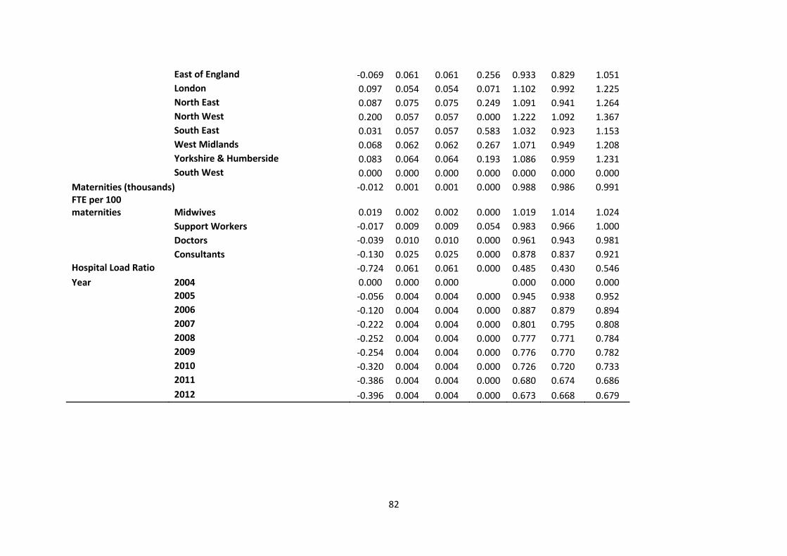
82

East of England -0.069 0.061 0.061 0.256 0.933 0.829 1.051

London 0.097 0.054 0.054 0.071 1.102 0.992 1.225

North East 0.087 0.075 0.075 0.249 1.091 0.941 1.264

North West 0.200 0.057 0.057 0.000 1.222 1.092 1.367

South East 0.031 0.057 0.057 0.583 1.032 0.923 1.153

West Midlands 0.068 0.062 0.062 0.267 1.071 0.949 1.208

Yorkshire & Humberside 0.083 0.064 0.064 0.193 1.086 0.959 1.231

South West 0.000 0.000 0.000 0.000 0.000 0.000 0.000

Maternities (thousands) -0.012 0.001 0.001 0.000 0.988 0.986 0.991 FTE per 100 maternities Midwives 0.019 0.002 0.002 0.000 1.019 1.014 1.024

Support Workers -0.017 0.009 0.009 0.054 0.983 0.966 1.000

Doctors -0.039 0.010 0.010 0.000 0.961 0.943 0.981

Consultants -0.130 0.025 0.025 0.000 0.878 0.837 0.921

Hospital Load Ratio -0.724 0.061 0.061 0.000 0.485 0.430 0.546

Year 2004 0.000 0.000 0.000

0.000 0.000 0.000

2005 -0.056 0.004 0.004 0.000 0.945 0.938 0.952

2006 -0.120 0.004 0.004 0.000 0.887 0.879 0.894

2007 -0.222 0.004 0.004 0.000 0.801 0.795 0.808

2008 -0.252 0.004 0.004 0.000 0.777 0.771 0.784

2009 -0.254 0.004 0.004 0.000 0.776 0.770 0.782

2010 -0.320 0.004 0.004 0.000 0.726 0.720 0.733

2011 -0.386 0.004 0.004 0.000 0.680 0.674 0.686

2012 -0.396 0.004 0.004 0.000 0.673 0.668 0.679

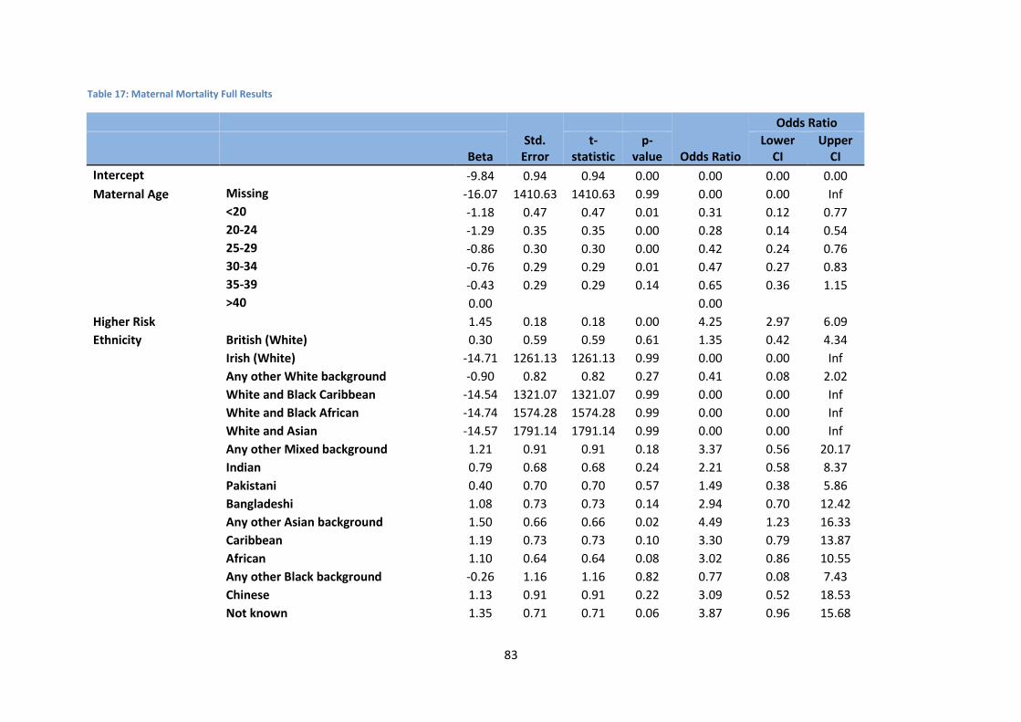
83

Table 17: Maternal Mortality Full Results

Std. Error

Odds Ratio

Odds Ratio

Beta t-

statistic p-

value Lower

CI Upper

CI

Intercept

-9.84 0.94 0.94 0.00 0.00 0.00 0.00

Maternal Age Missing -16.07 1410.63 1410.63 0.99 0.00 0.00 Inf

<20 -1.18 0.47 0.47 0.01 0.31 0.12 0.77

20-24 -1.29 0.35 0.35 0.00 0.28 0.14 0.54

25-29 -0.86 0.30 0.30 0.00 0.42 0.24 0.76

30-34 -0.76 0.29 0.29 0.01 0.47 0.27 0.83

35-39 -0.43 0.29 0.29 0.14 0.65 0.36 1.15

>40 0.00

0.00 Higher Risk

1.45 0.18 0.18 0.00 4.25 2.97 6.09

Ethnicity British (White) 0.30 0.59 0.59 0.61 1.35 0.42 4.34

Irish (White) -14.71 1261.13 1261.13 0.99 0.00 0.00 Inf

Any other White background -0.90 0.82 0.82 0.27 0.41 0.08 2.02

White and Black Caribbean -14.54 1321.07 1321.07 0.99 0.00 0.00 Inf

White and Black African -14.74 1574.28 1574.28 0.99 0.00 0.00 Inf

White and Asian -14.57 1791.14 1791.14 0.99 0.00 0.00 Inf

Any other Mixed background 1.21 0.91 0.91 0.18 3.37 0.56 20.17

Indian 0.79 0.68 0.68 0.24 2.21 0.58 8.37

Pakistani 0.40 0.70 0.70 0.57 1.49 0.38 5.86

Bangladeshi 1.08 0.73 0.73 0.14 2.94 0.70 12.42

Any other Asian background 1.50 0.66 0.66 0.02 4.49 1.23 16.33

Caribbean 1.19 0.73 0.73 0.10 3.30 0.79 13.87

African 1.10 0.64 0.64 0.08 3.02 0.86 10.55

Any other Black background -0.26 1.16 1.16 0.82 0.77 0.08 7.43

Chinese 1.13 0.91 0.91 0.22 3.09 0.52 18.53

Not known 1.35 0.71 0.71 0.06 3.87 0.96 15.68

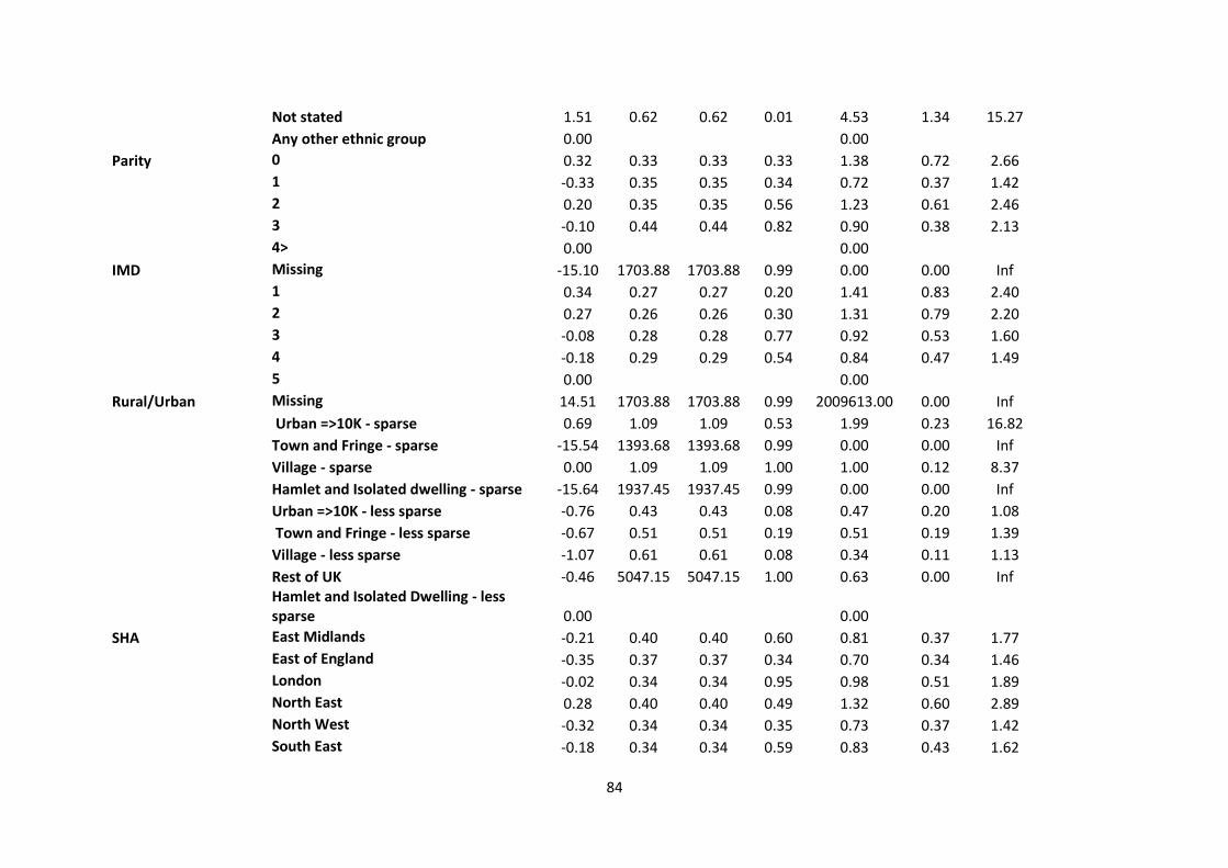
84

Not stated 1.51 0.62 0.62 0.01 4.53 1.34 15.27

Any other ethnic group 0.00

0.00

Parity 0 0.32 0.33 0.33 0.33 1.38 0.72 2.66

1 -0.33 0.35 0.35 0.34 0.72 0.37 1.42

2 0.20 0.35 0.35 0.56 1.23 0.61 2.46

3 -0.10 0.44 0.44 0.82 0.90 0.38 2.13

4> 0.00

0.00 IMD Missing -15.10 1703.88 1703.88 0.99 0.00 0.00 Inf

1 0.34 0.27 0.27 0.20 1.41 0.83 2.40

2 0.27 0.26 0.26 0.30 1.31 0.79 2.20

3 -0.08 0.28 0.28 0.77 0.92 0.53 1.60

4 -0.18 0.29 0.29 0.54 0.84 0.47 1.49

5 0.00

0.00 Rural/Urban Missing 14.51 1703.88 1703.88 0.99 2009613.00 0.00 Inf

Urban =>10K - sparse 0.69 1.09 1.09 0.53 1.99 0.23 16.82

Town and Fringe - sparse -15.54 1393.68 1393.68 0.99 0.00 0.00 Inf

Village - sparse 0.00 1.09 1.09 1.00 1.00 0.12 8.37

Hamlet and Isolated dwelling - sparse -15.64 1937.45 1937.45 0.99 0.00 0.00 Inf

Urban =>10K - less sparse -0.76 0.43 0.43 0.08 0.47 0.20 1.08

Town and Fringe - less sparse -0.67 0.51 0.51 0.19 0.51 0.19 1.39

Village - less sparse -1.07 0.61 0.61 0.08 0.34 0.11 1.13

Rest of UK -0.46 5047.15 5047.15 1.00 0.63 0.00 Inf

Hamlet and Isolated Dwelling - less sparse 0.00

0.00

SHA East Midlands -0.21 0.40 0.40 0.60 0.81 0.37 1.77

East of England -0.35 0.37 0.37 0.34 0.70 0.34 1.46

London -0.02 0.34 0.34 0.95 0.98 0.51 1.89

North East 0.28 0.40 0.40 0.49 1.32 0.60 2.89

North West -0.32 0.34 0.34 0.35 0.73 0.37 1.42

South East -0.18 0.34 0.34 0.59 0.83 0.43 1.62

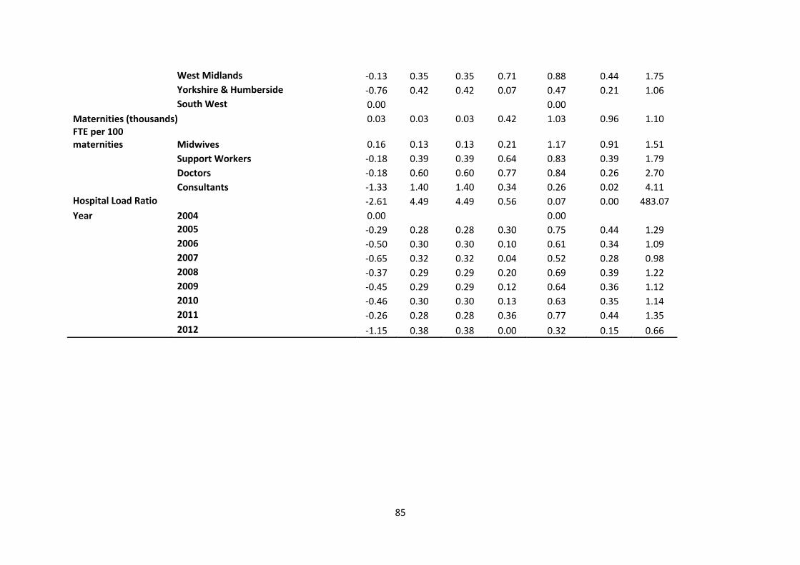
85

West Midlands -0.13 0.35 0.35 0.71 0.88 0.44 1.75

Yorkshire & Humberside -0.76 0.42 0.42 0.07 0.47 0.21 1.06

South West 0.00

0.00 Maternities (thousands) 0.03 0.03 0.03 0.42 1.03 0.96 1.10

FTE per 100 maternities Midwives 0.16 0.13 0.13 0.21 1.17 0.91 1.51

Support Workers -0.18 0.39 0.39 0.64 0.83 0.39 1.79

Doctors -0.18 0.60 0.60 0.77 0.84 0.26 2.70

Consultants -1.33 1.40 1.40 0.34 0.26 0.02 4.11

Hospital Load Ratio -2.61 4.49 4.49 0.56 0.07 0.00 483.07

Year 2004 0.00

0.00

2005 -0.29 0.28 0.28 0.30 0.75 0.44 1.29

2006 -0.50 0.30 0.30 0.10 0.61 0.34 1.09

2007 -0.65 0.32 0.32 0.04 0.52 0.28 0.98

2008 -0.37 0.29 0.29 0.20 0.69 0.39 1.22

2009 -0.45 0.29 0.29 0.12 0.64 0.36 1.12

2010 -0.46 0.30 0.30 0.13 0.63 0.35 1.14

2011 -0.26 0.28 0.28 0.36 0.77 0.44 1.35

2012 -1.15 0.38 0.38 0.00 0.32 0.15 0.66

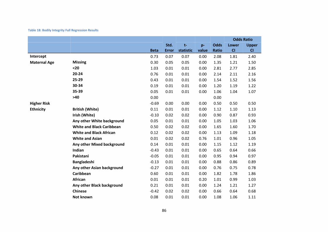
86

Table 18: Bodily Integrity Full Regression Results

Std. Error

Odds Ratio

Odds Ratio

Beta t-

statistic p-

value Lower

CI Upper

CI

Intercept

0.73 0.07 0.07 0.00 2.08 1.81 2.40

Maternal Age Missing 0.30 0.05 0.05 0.00 1.35 1.21 1.50

<20 1.03 0.01 0.01 0.00 2.81 2.77 2.85

20-24 0.76 0.01 0.01 0.00 2.14 2.11 2.16

25-29 0.43 0.01 0.01 0.00 1.54 1.52 1.56

30-34 0.19 0.01 0.01 0.00 1.20 1.19 1.22

35-39 0.05 0.01 0.01 0.00 1.06 1.04 1.07

>40 0.00

0.00 Higher Risk

-0.69 0.00 0.00 0.00 0.50 0.50 0.50

Ethnicity British (White) 0.11 0.01 0.01 0.00 1.12 1.10 1.13

Irish (White) -0.10 0.02 0.02 0.00 0.90 0.87 0.93

Any other White background 0.05 0.01 0.01 0.00 1.05 1.03 1.06

White and Black Caribbean 0.50 0.02 0.02 0.00 1.65 1.60 1.70

White and Black African 0.12 0.02 0.02 0.00 1.13 1.09 1.18

White and Asian 0.01 0.02 0.02 0.76 1.01 0.96 1.05

Any other Mixed background 0.14 0.01 0.01 0.00 1.15 1.12 1.19

Indian -0.43 0.01 0.01 0.00 0.65 0.64 0.66

Pakistani -0.05 0.01 0.01 0.00 0.95 0.94 0.97

Bangladeshi -0.13 0.01 0.01 0.00 0.88 0.86 0.89

Any other Asian background -0.27 0.01 0.01 0.00 0.76 0.75 0.78

Caribbean 0.60 0.01 0.01 0.00 1.82 1.78 1.86

African 0.01 0.01 0.01 0.20 1.01 0.99 1.03

Any other Black background 0.21 0.01 0.01 0.00 1.24 1.21 1.27

Chinese -0.42 0.02 0.02 0.00 0.66 0.64 0.68

Not known 0.08 0.01 0.01 0.00 1.08 1.06 1.11

87

Not stated 0.07 0.01 0.01 0.00 1.07 1.05 1.09

Any other ethnic group 0.00

0.00

Parity 0 -2.38 0.01 0.01 0.00 0.09 0.09 0.09

1 -1.28 0.01 0.01 0.00 0.28 0.28 0.28

2 -0.65 0.01 0.01 0.00 0.52 0.52 0.53

3 -0.29 0.01 0.01 0.00 0.74 0.74 0.75

4> 0.00

0.00 IMD Missing 0.26 0.02 0.02 0.00 1.30 1.24 1.36

1 0.46 0.00 0.00 0.00 1.58 1.56 1.59

2 0.30 0.00 0.00 0.00 1.36 1.35 1.37

3 0.19 0.00 0.00 0.00 1.20 1.19 1.21

4 0.10 0.00 0.00 0.00 1.10 1.09 1.11

5 0.00

0.00 Rural/Urban Missing

Urban =>10K - sparse 0.04 0.03 0.03 0.15 1.04 0.99 1.09

Town and Fringe - sparse 0.06 0.02 0.02 0.00 1.06 1.02 1.10

Village - sparse 0.04 0.02 0.02 0.06 1.04 1.00 1.08

Hamlet and Isolated dwelling - sparse -0.05 0.03 0.03 0.04 0.95 0.90 1.00

Urban =>10K - less sparse 0.03 0.01 0.01 0.00 1.03 1.01 1.05

Town and Fringe - less sparse 0.04 0.01 0.01 0.00 1.04 1.03 1.06

Village - less sparse 0.02 0.01 0.01 0.02 1.02 1.00 1.04

Rest of UK 0.13 0.06 0.06 0.04 1.14 1.00 1.29

Hamlet and Isolated Dwelling - less sparse 0.00

0.00

SHA East Midlands 0.14 0.11 0.11 0.20 1.15 0.93 1.42

East of England -0.12 0.09 0.09 0.20 0.89 0.74 1.07

London -0.24 0.08 0.08 0.01 0.79 0.67 0.93

North East 0.11 0.12 0.12 0.33 1.12 0.89 1.41

North West -0.10 0.09 0.09 0.26 0.90 0.76 1.08

South East -0.15 0.09 0.09 0.08 0.86 0.72 1.02

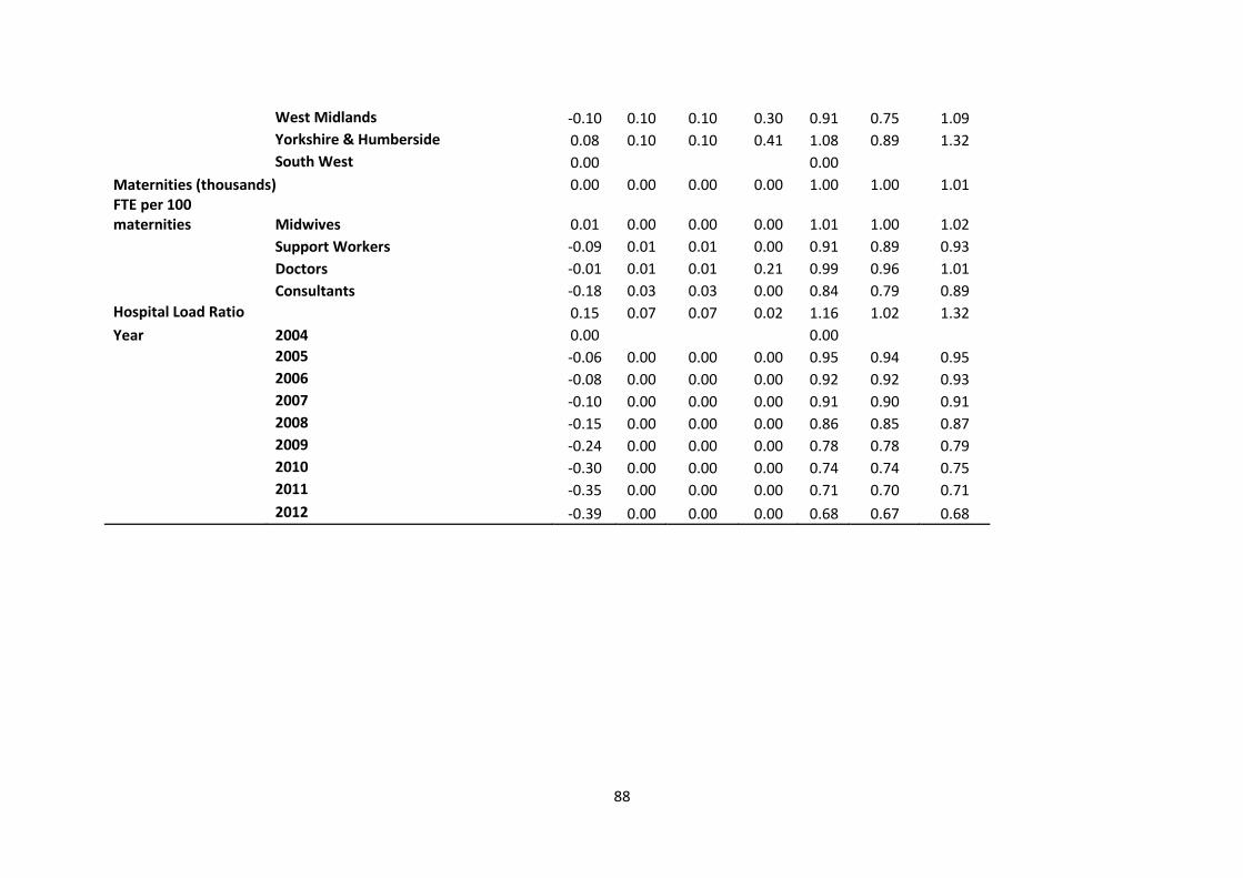
88

West Midlands -0.10 0.10 0.10 0.30 0.91 0.75 1.09

Yorkshire & Humberside 0.08 0.10 0.10 0.41 1.08 0.89 1.32

South West 0.00

0.00 Maternities (thousands) 0.00 0.00 0.00 0.00 1.00 1.00 1.01

FTE per 100 maternities Midwives 0.01 0.00 0.00 0.00 1.01 1.00 1.02

Support Workers -0.09 0.01 0.01 0.00 0.91 0.89 0.93

Doctors -0.01 0.01 0.01 0.21 0.99 0.96 1.01

Consultants -0.18 0.03 0.03 0.00 0.84 0.79 0.89

Hospital Load Ratio 0.15 0.07 0.07 0.02 1.16 1.02 1.32

Year 2004 0.00

0.00

2005 -0.06 0.00 0.00 0.00 0.95 0.94 0.95

2006 -0.08 0.00 0.00 0.00 0.92 0.92 0.93

2007 -0.10 0.00 0.00 0.00 0.91 0.90 0.91

2008 -0.15 0.00 0.00 0.00 0.86 0.85 0.87

2009 -0.24 0.00 0.00 0.00 0.78 0.78 0.79

2010 -0.30 0.00 0.00 0.00 0.74 0.74 0.75

2011 -0.35 0.00 0.00 0.00 0.71 0.70 0.71

2012 -0.39 0.00 0.00 0.00 0.68 0.67 0.68

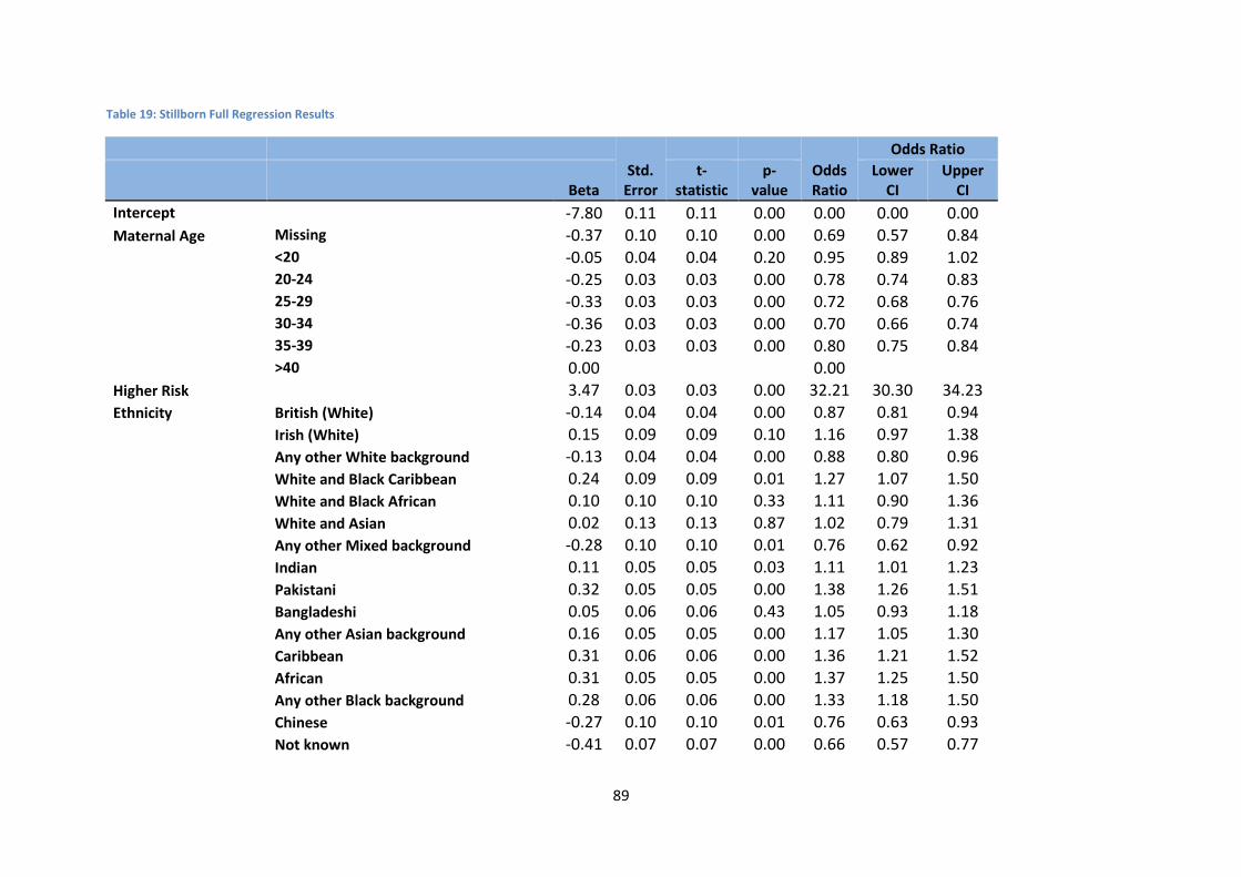
89

Table 19: Stillborn Full Regression Results

Std. Error

Odds Ratio

Odds Ratio

Beta t-

statistic p-

value Lower

CI Upper

CI

Intercept

-7.80 0.11 0.11 0.00 0.00 0.00 0.00

Maternal Age Missing -0.37 0.10 0.10 0.00 0.69 0.57 0.84

<20 -0.05 0.04 0.04 0.20 0.95 0.89 1.02

20-24 -0.25 0.03 0.03 0.00 0.78 0.74 0.83

25-29 -0.33 0.03 0.03 0.00 0.72 0.68 0.76

30-34 -0.36 0.03 0.03 0.00 0.70 0.66 0.74

35-39 -0.23 0.03 0.03 0.00 0.80 0.75 0.84

>40 0.00

0.00 Higher Risk

3.47 0.03 0.03 0.00 32.21 30.30 34.23

Ethnicity British (White) -0.14 0.04 0.04 0.00 0.87 0.81 0.94

Irish (White) 0.15 0.09 0.09 0.10 1.16 0.97 1.38

Any other White background -0.13 0.04 0.04 0.00 0.88 0.80 0.96

White and Black Caribbean 0.24 0.09 0.09 0.01 1.27 1.07 1.50

White and Black African 0.10 0.10 0.10 0.33 1.11 0.90 1.36

White and Asian 0.02 0.13 0.13 0.87 1.02 0.79 1.31

Any other Mixed background -0.28 0.10 0.10 0.01 0.76 0.62 0.92

Indian 0.11 0.05 0.05 0.03 1.11 1.01 1.23

Pakistani 0.32 0.05 0.05 0.00 1.38 1.26 1.51

Bangladeshi 0.05 0.06 0.06 0.43 1.05 0.93 1.18

Any other Asian background 0.16 0.05 0.05 0.00 1.17 1.05 1.30

Caribbean 0.31 0.06 0.06 0.00 1.36 1.21 1.52

African 0.31 0.05 0.05 0.00 1.37 1.25 1.50

Any other Black background 0.28 0.06 0.06 0.00 1.33 1.18 1.50

Chinese -0.27 0.10 0.10 0.01 0.76 0.63 0.93

Not known -0.41 0.07 0.07 0.00 0.66 0.57 0.77

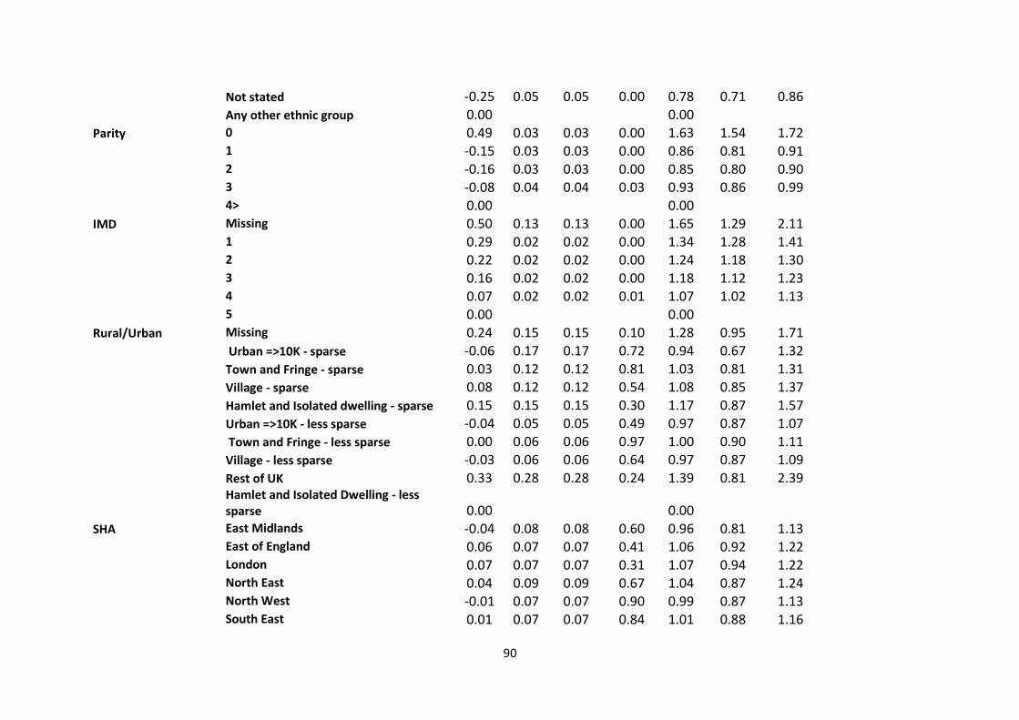
90

Not stated -0.25 0.05 0.05 0.00 0.78 0.71 0.86

Any other ethnic group 0.00

0.00

Parity 0 0.49 0.03 0.03 0.00 1.63 1.54 1.72

1 -0.15 0.03 0.03 0.00 0.86 0.81 0.91

2 -0.16 0.03 0.03 0.00 0.85 0.80 0.90

3 -0.08 0.04 0.04 0.03 0.93 0.86 0.99

4> 0.00

0.00 IMD Missing 0.50 0.13 0.13 0.00 1.65 1.29 2.11

1 0.29 0.02 0.02 0.00 1.34 1.28 1.41

2 0.22 0.02 0.02 0.00 1.24 1.18 1.30

3 0.16 0.02 0.02 0.00 1.18 1.12 1.23

4 0.07 0.02 0.02 0.01 1.07 1.02 1.13

5 0.00

0.00 Rural/Urban Missing 0.24 0.15 0.15 0.10 1.28 0.95 1.71

Urban =>10K - sparse -0.06 0.17 0.17 0.72 0.94 0.67 1.32

Town and Fringe - sparse 0.03 0.12 0.12 0.81 1.03 0.81 1.31

Village - sparse 0.08 0.12 0.12 0.54 1.08 0.85 1.37

Hamlet and Isolated dwelling - sparse 0.15 0.15 0.15 0.30 1.17 0.87 1.57

Urban =>10K - less sparse -0.04 0.05 0.05 0.49 0.97 0.87 1.07

Town and Fringe - less sparse 0.00 0.06 0.06 0.97 1.00 0.90 1.11

Village - less sparse -0.03 0.06 0.06 0.64 0.97 0.87 1.09

Rest of UK 0.33 0.28 0.28 0.24 1.39 0.81 2.39

Hamlet and Isolated Dwelling - less sparse 0.00

0.00

SHA East Midlands -0.04 0.08 0.08 0.60 0.96 0.81 1.13

East of England 0.06 0.07 0.07 0.41 1.06 0.92 1.22

London 0.07 0.07 0.07 0.31 1.07 0.94 1.22

North East 0.04 0.09 0.09 0.67 1.04 0.87 1.24

North West -0.01 0.07 0.07 0.90 0.99 0.87 1.13

South East 0.01 0.07 0.07 0.84 1.01 0.88 1.16

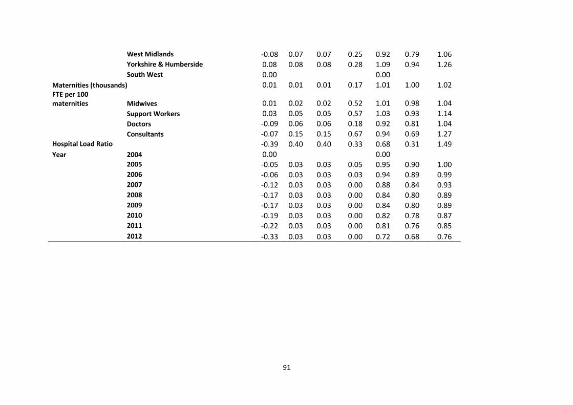
91

West Midlands -0.08 0.07 0.07 0.25 0.92 0.79 1.06

Yorkshire & Humberside 0.08 0.08 0.08 0.28 1.09 0.94 1.26

South West 0.00

0.00 Maternities (thousands) 0.01 0.01 0.01 0.17 1.01 1.00 1.02

FTE per 100 maternities Midwives 0.01 0.02 0.02 0.52 1.01 0.98 1.04

Support Workers 0.03 0.05 0.05 0.57 1.03 0.93 1.14

Doctors -0.09 0.06 0.06 0.18 0.92 0.81 1.04

Consultants -0.07 0.15 0.15 0.67 0.94 0.69 1.27

Hospital Load Ratio -0.39 0.40 0.40 0.33 0.68 0.31 1.49

Year 2004 0.00

0.00

2005 -0.05 0.03 0.03 0.05 0.95 0.90 1.00

2006 -0.06 0.03 0.03 0.03 0.94 0.89 0.99

2007 -0.12 0.03 0.03 0.00 0.88 0.84 0.93

2008 -0.17 0.03 0.03 0.00 0.84 0.80 0.89

2009 -0.17 0.03 0.03 0.00 0.84 0.80 0.89

2010 -0.19 0.03 0.03 0.00 0.82 0.78 0.87

2011 -0.22 0.03 0.03 0.00 0.81 0.76 0.85

2012 -0.33 0.03 0.03 0.00 0.72 0.68 0.76

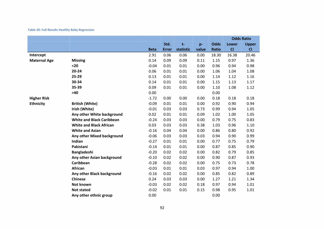
92

Table 20: Full Results Healthy Baby Regression

Std. Error

Odds Ratio

Odds Ratio

Beta t-

statistic p-

value Lower

CI Upper

CI

Intercept

2.91 0.06 0.06 0.00 18.30 16.38 20.46

Maternal Age Missing 0.14 0.09 0.09 0.11 1.15 0.97 1.36

<20 -0.04 0.01 0.01 0.00 0.96 0.94 0.98

20-24 0.06 0.01 0.01 0.00 1.06 1.04 1.08

25-29 0.13 0.01 0.01 0.00 1.14 1.12 1.16

30-34 0.14 0.01 0.01 0.00 1.15 1.13 1.17

35-39 0.09 0.01 0.01 0.00 1.10 1.08 1.12

>40 0.00

0.00

Higher Risk

-1.72 0.00 0.00 0.00 0.18 0.18 0.18

Ethnicity British (White) -0.09 0.01 0.01 0.00 0.92 0.90 0.94

Irish (White) -0.01 0.03 0.03 0.73 0.99 0.94 1.05

Any other White background 0.02 0.01 0.01 0.09 1.02 1.00 1.05

White and Black Caribbean -0.24 0.03 0.03 0.00 0.79 0.75 0.83

White and Black African 0.03 0.03 0.03 0.38 1.03 0.96 1.10

White and Asian -0.16 0.04 0.04 0.00 0.86 0.80 0.92

Any other Mixed background -0.06 0.03 0.03 0.03 0.94 0.90 0.99

Indian -0.27 0.01 0.01 0.00 0.77 0.75 0.79

Pakistani -0.14 0.01 0.01 0.00 0.87 0.85 0.90

Bangladeshi -0.20 0.02 0.02 0.00 0.82 0.79 0.85

Any other Asian background -0.10 0.02 0.02 0.00 0.90 0.87 0.93

Caribbean -0.28 0.02 0.02 0.00 0.75 0.73 0.78

African -0.03 0.01 0.01 0.03 0.97 0.94 1.00

Any other Black background -0.16 0.02 0.02 0.00 0.85 0.82 0.89

Chinese 0.24 0.03 0.03 0.00 1.27 1.21 1.34

Not known -0.03 0.02 0.02 0.18 0.97 0.94 1.01

Not stated -0.02 0.01 0.01 0.15 0.98 0.95 1.01

Any other ethnic group 0.00

0.00

93

Parity 0 -0.22 0.01 0.01 0.00 0.80 0.79 0.82

1 0.25 0.01 0.01 0.00 1.29 1.27 1.31

2 0.22 0.01 0.01 0.00 1.25 1.23 1.27

3 0.12 0.01 0.01 0.00 1.13 1.11 1.15

4> 0.00

0.00

IMD Missing -0.42 0.03 0.03 0.00 0.65 0.61 0.70

1 -0.25 0.01 0.01 0.00 0.78 0.77 0.79

2 -0.17 0.01 0.01 0.00 0.84 0.83 0.86

3 -0.11 0.01 0.01 0.00 0.89 0.88 0.90

4 -0.06 0.01 0.01 0.00 0.94 0.93 0.95

5 0.00

0.00

Rural/Urban Missing

Urban =>10K - sparse -0.16 0.05 0.05 0.00 0.85 0.78 0.93

Town and Fringe - sparse -0.07 0.03 0.03 0.02 0.93 0.87 0.99

Village - sparse 0.00 0.03 0.03 0.96 1.00 0.94 1.07

Hamlet and Isolated dwelling - sparse 0.02 0.04 0.04 0.66 1.02 0.94 1.11

Urban =>10K - less sparse -0.03 0.01 0.01 0.01 0.97 0.94 0.99

Town and Fringe - less sparse -0.04 0.01 0.01 0.01 0.96 0.93 0.99

Village - less sparse 0.01 0.02 0.02 0.41 1.01 0.98 1.04

Rest of UK -0.47 0.08 0.08 0.00 0.62 0.53 0.73

Hamlet and Isolated Dwelling - less sparse 0.00

0.00

SHA East Midlands 0.40 0.08 0.08 0.00 1.49 1.28 1.74

East of England 0.25 0.07 0.07 0.00 1.28 1.12 1.46

London 0.26 0.06 0.06 0.00 1.29 1.15 1.46

North East 0.28 0.08 0.08 0.00 1.33 1.13 1.56

North West 0.29 0.06 0.06 0.00 1.34 1.18 1.52

South East 0.29 0.06 0.06 0.00 1.34 1.18 1.52

West Midlands 0.28 0.07 0.07 0.00 1.33 1.16 1.52

Yorkshire & Humberside 0.21 0.07 0.07 0.00 1.24 1.08 1.42

South West 0.00

0.00

Maternities (thousands) 0.00 0.00 0.00 0.34 1.00 1.00 1.01

94

FTE per 100 maternities Midwives 0.00 0.00 0.00 0.92 1.00 0.99 1.01

Support Workers -0.05 0.02 0.02 0.00 0.95 0.92 0.98

Doctors -0.03 0.02 0.02 0.19 0.97 0.94 1.01

Consultants 0.09 0.05 0.05 0.07 1.10 0.99 1.21

Hospital Load Ratio 0.28 0.11 0.11 0.02 1.32 1.05 1.65

Year 2004 0.00

0.00

2005 0.05 0.01 0.01 0.00 1.05 1.04 1.07

2006 0.06 0.01 0.01 0.00 1.06 1.04 1.07

2007 0.10 0.01 0.01 0.00 1.10 1.09 1.12

2008 0.13 0.01 0.01 0.00 1.14 1.12 1.16

2009 0.13 0.01 0.01 0.00 1.14 1.13 1.16

2010 0.17 0.01 0.01 0.00 1.19 1.17 1.21

2011 0.21 0.01 0.01 0.00 1.24 1.22 1.26

2012 0.25 0.01 0.01 0.00 1.28 1.26 1.30

Table 21: Healthy Baby Full Regression Results

Std. Error

Odds Ratio

Odds Ratio

Beta t- p- Lower Upper

95

statistic value CI CI

Intercept

2.91 0.06 0.06 0.00 18.30 16.38 20.46

Maternal Age Missing 0.14 0.09 0.09 0.11 1.15 0.97 1.36

<20 -0.04 0.01 0.01 0.00 0.96 0.94 0.98

20-24 0.06 0.01 0.01 0.00 1.06 1.04 1.08

25-29 0.13 0.01 0.01 0.00 1.14 1.12 1.16

30-34 0.14 0.01 0.01 0.00 1.15 1.13 1.17

35-39 0.09 0.01 0.01 0.00 1.10 1.08 1.12

>40 0.00

0.00

Higher Risk

-1.72 0.00 0.00 0.00 0.18 0.18 0.18

Ethnicity British (White) -0.09 0.01 0.01 0.00 0.92 0.90 0.94

Irish (White) -0.01 0.03 0.03 0.73 0.99 0.94 1.05

Any other White background 0.02 0.01 0.01 0.09 1.02 1.00 1.05

White and Black Caribbean -0.24 0.03 0.03 0.00 0.79 0.75 0.83

White and Black African 0.03 0.03 0.03 0.38 1.03 0.96 1.10

White and Asian -0.16 0.04 0.04 0.00 0.86 0.80 0.92

Any other Mixed background -0.06 0.03 0.03 0.03 0.94 0.90 0.99

Indian -0.27 0.01 0.01 0.00 0.77 0.75 0.79

Pakistani -0.14 0.01 0.01 0.00 0.87 0.85 0.90

Bangladeshi -0.20 0.02 0.02 0.00 0.82 0.79 0.85

Any other Asian background -0.10 0.02 0.02 0.00 0.90 0.87 0.93

Caribbean -0.28 0.02 0.02 0.00 0.75 0.73 0.78

African -0.03 0.01 0.01 0.03 0.97 0.94 1.00

Any other Black background -0.16 0.02 0.02 0.00 0.85 0.82 0.89

Chinese 0.24 0.03 0.03 0.00 1.27 1.21 1.34

Not known -0.03 0.02 0.02 0.18 0.97 0.94 1.01

Not stated -0.02 0.01 0.01 0.15 0.98 0.95 1.01

Any other ethnic group 0.00

0.00

Parity 0 -0.22 0.01 0.01 0.00 0.80 0.79 0.82

1 0.25 0.01 0.01 0.00 1.29 1.27 1.31

2 0.22 0.01 0.01 0.00 1.25 1.23 1.27

3 0.12 0.01 0.01 0.00 1.13 1.11 1.15

96

4> 0.00

0.00

IMD Missing -0.42 0.03 0.03 0.00 0.65 0.61 0.70

1 -0.25 0.01 0.01 0.00 0.78 0.77 0.79

2 -0.17 0.01 0.01 0.00 0.84 0.83 0.86

3 -0.11 0.01 0.01 0.00 0.89 0.88 0.90

4 -0.06 0.01 0.01 0.00 0.94 0.93 0.95

5 0.00

0.00 Rural/Urban Missing

Urban =>10K - sparse -0.16 0.05 0.05 0.00 0.85 0.78 0.93

Town and Fringe - sparse -0.07 0.03 0.03 0.02 0.93 0.87 0.99

Village - sparse 0.00 0.03 0.03 0.96 1.00 0.94 1.07

Hamlet and Isolated dwelling - sparse 0.02 0.04 0.04 0.66 1.02 0.94 1.11

Urban =>10K - less sparse -0.03 0.01 0.01 0.01 0.97 0.94 0.99

Town and Fringe - less sparse -0.04 0.01 0.01 0.01 0.96 0.93 0.99

Village - less sparse 0.01 0.02 0.02 0.41 1.01 0.98 1.04

Rest of UK -0.47 0.08 0.08 0.00 0.62 0.53 0.73

Hamlet and Isolated Dwelling - less sparse 0.00

0.00

SHA East Midlands 0.40 0.08 0.08 0.00 1.49 1.28 1.74

East of England 0.25 0.07 0.07 0.00 1.28 1.12 1.46

London 0.26 0.06 0.06 0.00 1.29 1.15 1.46

North East 0.28 0.08 0.08 0.00 1.33 1.13 1.56

North West 0.29 0.06 0.06 0.00 1.34 1.18 1.52

South East 0.29 0.06 0.06 0.00 1.34 1.18 1.52

West Midlands 0.28 0.07 0.07 0.00 1.33 1.16 1.52

Yorkshire & Humberside 0.21 0.07 0.07 0.00 1.24 1.08 1.42

South West 0.00

0.00

Maternities (thousands) 0.00 0.00 0.00 0.34 1.00 1.00 1.01 FTE per 100 maternities Midwives 0.00 0.00 0.00 0.92 1.00 0.99 1.01

Support Workers -0.05 0.02 0.02 0.00 0.95 0.92 0.98

Doctors -0.03 0.02 0.02 0.19 0.97 0.94 1.01

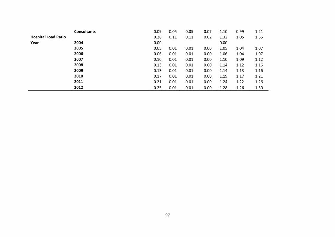
97

Consultants 0.09 0.05 0.05 0.07 1.10 0.99 1.21

Hospital Load Ratio 0.28 0.11 0.11 0.02 1.32 1.05 1.65

Year 2004 0.00

0.00

2005 0.05 0.01 0.01 0.00 1.05 1.04 1.07

2006 0.06 0.01 0.01 0.00 1.06 1.04 1.07

2007 0.10 0.01 0.01 0.00 1.10 1.09 1.12

2008 0.13 0.01 0.01 0.00 1.14 1.12 1.16

2009 0.13 0.01 0.01 0.00 1.14 1.13 1.16

2010 0.17 0.01 0.01 0.00 1.19 1.17 1.21

2011 0.21 0.01 0.01 0.00 1.24 1.22 1.26

2012 0.25 0.01 0.01 0.00 1.28 1.26 1.30