the cooke triplet and tessar lenses - welcome to … · 324 chapter b.3 the cooke triplet and...

323

Chapter B.3

The Cooke Triplet and Tessar Lenses

Following the introduction of photography in 1839, the development of cam-era lenses progressed in an evolutionary way with occasional revolutions. Almostimmediately, the singlet meniscus Landscape lens was achromatized, thus becom-ing a cemented doublet meniscus. Soon afterward, pairs of either singlet or dou-blet menisci were combined symmetrically about a stop. The most successful ofthe double-doublets was the Rapid Rectilinear lens, introduced in 1866. This useof symmetry was then further extended to pairs of menisci, with each meniscusconsisting of three, four, or even five elements cemented together. The most suc-cessful of these lenses was the Dagor, a double-triplet (six elements), introducedin 1892. The Dagor and some of its variants are still in use today.

The first revolution or major innovation occurred in 1840 by Joseph Petzvalwith his introduction of mathematically designed lenses. Petzval’s most famouslens is the Petzval Portrait lens. The Petzval lens is not symmetrical and has majoraberrations off-axis (most noticeably, field curvature). Nevertheless, in 1840 itwas an immediate success, not least because at f/3.6 it was 20 times faster (trans-mitted 20 times more light) than the f/16 Landscape lens, its only competition atthe time. Petzval type lenses were widely used until well into the twentieth cen-tury, and they are sometimes still encountered, especially in projectors.

The second revolution, which began in 1886, was the development of newtypes of optical glass, especially the high-index crowns. These glasses made pos-sible the first anastigmatic lenses; that is, lenses with astigmatism corrected on aflat field.

The third revolution was the invention by H. Dennis Taylor in 1893 of theCooke Triplet lens (Cooke was Taylor’s employer). A Cooke Triplet consists oftwo positive singlet elements and one negative singlet element, all of which canbe thin. Two sizable airspaces separate the three elements. The negative elementis located in the middle about halfway between the positive elements, thus main-taining a large amount of symmetry. By this approach, Taylor found that he couldaccomplish with only three elements what others required six, eight, or ten ele-

324 Chapter B.3 The Cooke Triplet and Tessar Lenses

ments to do when using pairs of cemented menisci. After more than a century, theCooke Triplet remains one of the most popular camera lens forms.

The design and performance of a Cooke Triplet is the main subject of thischapter. The construction of a Cooke Triplet is illustrated in Figure B.3.1.1. Alsoincluded here for comparison is a Tessar lens, which can be considered a deriva-tive and extension of the Cooke Triplet (although Paul Rudolph designed the firstTessar in 1902 as a modification of an earlier anastigmat, the Protar).

The development of camera lenses has continued unabated to this day, witha huge number of evolutionary advances and several more revolutions (most no-tably, anti-reflection coatings and computer-aided optimization). The reader isencouraged to become familiar with optical history. It is a fascinating story.1

B.3.1 Lens Specifications

The lenses in this chapter are normal or standard lenses for a 35 mm type still(not movie) camera with the object at infinity. Note that 35 mm refers to the phys-

1 Optical history is discussed in many of the references listed in the bibliography. Three particularlygood sources are: Rudolf Kingslake, A History of the Photographic Lens; Henry C. King, The Historyof the Telescope; and Joseph Ashbrook, The Astronomical Scrapbook.

Figure B.3.1.1

Section B.3.2: Degrees of Freedom 325

ical width of the film, not to the image size, which is only 24 mm wide (and36 mm long). This image size was chosen for the first Leica camera in 1924 andhas been the standard ever since. The remaining film area is occupied by two setsof sprocket holes, a vestige from its origin as a motion picture film (where the im-age is only 18 mm long).

As mentioned in the previous chapter, a normal lens gives normal-perspec-tive photographs and has a focal length roughly equal to the image format diam-eter or diagonal. At 24x36 mm, the diagonal of the 35 mm format is 43.3 mm.However, the lens on the first Leica had a focal length of 50 mm, and again thisvalue has become standard. Actually, most normal lenses for 35 mm cameras aredeliberately designed to have a focal length even a bit longer still. Thus, althoughthe nominal focal length engraved on the lens barrel is 50 mm, the true focallength is often closer to 52 mm. Thus, 52.0 mm is adopted as the focal length forthe lenses in this chapter. This focal length is longer than the format diagonal, butit is close enough.

Given this focal length and image format, the diagonal field of view (fromcorner to corner) is 45.2º, or ±22.6º. Four field positions are used during optimi-zation and evaluation: 0º, 9º, 15.8º, and 22.6º (or 0, 40%, 70%, and 100% ofhalf-field). Object 1 is in the field center, object 4 is at the distance of the formatcorner, object 3 is at the distance of one side of an equivalent square format, andobject 2 is slightly greater than halfway between objects 1 and 3. Of course, foran ordinary camera lens, the field (image surface) is flat.

For a photographic Cooke Triplet covering this angular view, it is usuallynot practical to increase speed beyond about f/3.5. Triplets with focal lengths of52 mm and speeds of f/3.5 are widely manufactured and used with success. Thus,f/3.5 is adopted here.

During optimization, no special emphasis is given to the center of the pupilto the detriment of the pupil edges. To increase performance when stopped down,the lens is optimized and used on the paraxial focal plane. At the edge of the field,a reasonable amount of mechanical vignetting is allowed. Distortion is correctedto zero at the edge of the field.

Five wavelengths are used during optimization and evaluation. Becausemost films are sensitive to wavelengths between about 0.40 μm and 0.70 μm, thefive wavelengths are: 0.45, 0.50, 0.55, 0.60, and 0.65 μm. For panchromatic filmsensitivity, these wavelengths are weighted equally. The reference wavelength forcalculating first-order properties and solves is the central wavelength, 0.55 μm.

And finally, the performance criterion for the optimized lens is diffractionMTF; that is, the form of MTF with both diffraction and aberrations included.

B.3.2 Degrees of Freedom

The Cooke Triplet is a very interesting optical configuration.2 Refer again to


Figure B.3.1.1. There are exactly eight effective independent variables or degreesof freedom available for the control of optical properties. These major variablesare six lens surface curvatures and two interelement airspaces. The six curvaturescan also be viewed as three lens powers and three lens bendings.

Recall that there are seven basic or primary aberrations (first-order longitu-dinal and lateral color, and the five monochromatic third-order Seidel aberra-tions). Thus, the Cooke Triplet has just enough effective independent variables tocorrect all first- and third-order aberrations plus focal length.

Although the airspaces in a Cooke Triplet are effective variables, the glassthicknesses are unfortunately only weak, ineffective variables that somewhat du-plicate the airspaces. The glass center thicknesses are usually arbitrarily chosenfor ease of fabrication.

The three glass choices can also be viewed as variables (or index and disper-sion variable pairs). But the range of available glasses is limited, and the require-ments of achromatization further restrict the glasses. In practice, the role of glassselection is to determine which of a multitude of possible optical solutions youget.

Stop shift is not a degree of freedom. A Cooke Triplet is nearly symmetricalabout the middle element, which makes aberration control much easier. To retainas much symmetry as possible, the stop is either at the middle element or just toone side. A slightly separated stop allows the stop to be a variable iris diaphragmfor changing the f/number. Locating the iris to the rear of the middle element,rather than to the front, is more common, although both work. In the present ex-ample, the stop is 2 mm behind the middle element.

With only eight effective variables, there are no variables available for con-trolling the higher-order monochromatic aberrations that will inevitably bepresent. Although it is possible in a Cooke Triplet to correct all seven first- andthird-order aberrations exactly to zero, in practice this is never done. Controlledamounts of third-order aberrations are always deliberately left in to balance thefifth- and higher-orders. However, there is a limit to how well this cancellationworks. Thus, Cooke Triplets are usually restricted to applications requiring onlymoderate speed and field coverage; that is, where there are only moderateamounts of fifth- and higher-order aberrations. For higher performance, a lensconfiguration with a larger number of effective degrees of freedom is needed.

2 For those interested in the more analytical aspects of designing a Cooke Triplet lens, see the excel-lent discussions in: Warren J. Smith, Modern Optical Engineering, second edition, pp. 384-390; War-ren J. Smith, Modern Lens Design, pp. 123-146; and Rudolf Kingslake, Lens Design Fundamentals,pp. 286-295. These three books are also highly recommended for their discussions of many other top-ics in optics.

Section B.3.3: Glass Selection 327

B.3.3 Glass Selection

A Cooke Triplet is an achromat. Thus, as discussed in Chapter B.1, each ofthe two positive elements must be made of a crown type glass (lower dispersionor higher Abbe number), and the negative element must be made of a flint typeglass (higher dispersion or lower Abbe number).

For practical reasons, and with no loss of performance, both positive crownelements are usually made of the same glass type, and this will be done here.

The sizes of the airspaces in a Cooke Triplet are a strong function of the dis-persion difference between the crown and flint glasses. A dispersion differencethat is too small causes the lens elements to be jammed up against each other, andthere are also large aberrations. Conversely, a dispersion difference that is toolarge causes the system to be excessively stretched out, and again there are largeaberrations. One value of dispersion difference produces airspaces of the rightsize to yield a good optical solution. Fortunately, the required dispersion differ-ence can be satisfied by the range of actual available glasses on the glass map.

The difference in nd index of refraction between the crown and flint glassesalso enters into the optical solution. To help reduce the Petzval sum to flatten thefield, the positive elements should be made of a higher-index crown glass, and thenegative element should be made of a somewhat lower-index flint glass.

To make this an exercise in determining the capability of the Cooke Tripletdesign form, all the more or less normal glass types will be allowed. This includesall the expensive high-index lanthanum glasses. Glass cost should not be a drivingissue here because the lens elements are quite small and require only smallamounts of glass. Optical and machine shop fabrication costs should be muchmore important than glass cost. However, this is not true for all types of lenses;the relative importance of glass cost gets greater as element sizes get larger. Notethat no attempt is made here to reduce secondary color, and thus the abnormal-dis-persion glasses are excluded.

Experience has shown that high-index crown glasses generally give betterimage quality. Not only is the Petzval sum reduced, but high indices yield lowersurface curvatures that in turn reduce the higher-order aberrations. Because thereare relatively few high-index crowns on the glass map, the usual procedure whenselecting glasses for a Cooke Triplet is to first select the crown glass type, and tothen select the matching flint glass type from among the many possibilities.

Refer back to the glass map in Figure A.10.2. Note that the boundary of thehighest-index crowns is a nearly straight line on the upper left side extending from(in the Schott catalog) about SK16 (nd of 1.620, Vd of 60.3) to about LaSFN31 (nd

of 1.881, Vd of 41.0). Although the top of this line extends well into the nominallyflint glasses, the glasses along the top can function as crown glasses because theyare more crowny than the very flinty dense SF glasses with which they would bepaired.


The candidate crown glasses are therefore located along the line boundingthe upper left of the populated region of the glass map. An excellent crown glassof very high index is Schott LaFN21 (nd of 1.788, Vd of 47.5). Although not themost extreme high-index crown, LaFN21 is widely used and practical. Thus,LaFN21 is adopted here.

Given the crown glass selection, the basic optical design requires a matchingflint having a certain dispersion difference and a low index. However, there is alimit to how low the flint index can be. This limit is the arc bordering the rightand bottom of the populated region of the glass map (again see Figure A.10.2).This arc is called the old glass line. Thus, it is from the glasses along the old glassline that the flint glass of a Cooke Triplet is usually selected.

For early optimizations, make a guess at the flint glass type. Fortunately,your guess does not have to be very good because it will soon be revised. Accord-ingly, Schott SF15 (nd of 1.699, Vd of 30.1), a glass on the old glass line with anindex somewhat lower than LaFN21, is provisionally adopted.

For intermediate optimizations, the same crown glass selection, LaFN21, isretained, but a more optimum flint glass match must now be made. One way tofind the best flint is to let flint glass type be a variable during optimization and letthe computer make the selection. However, because some lens design programsmay have difficulty handling variable glasses, a manual approach may be moreeffective, and also more revealing to the lens designer.

Using the manual approach, select several likely flint glass candidates fromalong the old glass line to combine with LaFN21. For each combination, optimizethe Cooke Triplet with the intermediate merit function. Flint glasses down and tothe left on the glass line will yield lenses with smaller airspaces; flints up and tothe right will yield larger airspaces. Adjust the apertures to give roughly the re-quired amount of vignetting. For each of the combinations, tabulate the value ofthe merit function and look at the layout and ray fan plot. The best glass pair willshow a practical layout and have the lowest value of the merit function.

In the present Cooke Triplet example with the two crown elements made ofSchott LaFN21 (nd of 1.788, Vd of 47.5), the matching glass for the flint elementis found to be, not SF15 (nd of 1.699, Vd of 30.1) as was first guessed, but SchottSF53 (nd of 1.728, Vd of 28.7). Both LaFN21 and SF53 are among Schott’s pre-ferred glass types.

B.3.4 Flattening the Field

When choosing glasses, it is important to consider the Petzval sum. Referagain to the discussion of Petzval sum in Chapter A.9. Recall that the Petzval sumgives the curvature of the Petzval surface, and that (when only considering astig-matism and field curvature) the Petzval surface is the best image surface whenastigmatism is zero.

Section B.3.4: Flattening the Field 329

Thus, for a lens with little astigmatism, the Petzval sum must be made smallto flatten the field. However, the sum need not be exactly zero because leaving ina small amount of Petzval curvature allows field-dependent defocus to be addedto the off-axis aberration cancelling mix. The important thing is that the Petzvalsum must be controllable during optimization.

For thin lens elements, the contribution to the Petzval sum by a given ele-ment goes directly as element power and inversely as element index of refraction.In a multi-element lens with an overall positive focal length, the elements withpositive power necessarily predominate. Thus the Petzval sum will naturally tendto be sizable and negative, thereby giving an inward curving field (image surfaceconcave to the light).

There are in general two ways to reduce the Petzval sum to flatten the field.They are: (1) glass selection and (2) axial separation of positive and negative op-tical powers. In practice, both ways are usually used together. As was mentionedin the previous section, the first way, glass selection, requires that the two positiveelements of a Cooke Triplet be made of higher-index glass to give decreased neg-ative Petzval contributions, and the negative element be made of lower-indexglass to give an increased positive contribution. The second way, separation ofpowers, requires that the positive and negative elements be separated in a mannerthat causes the power of the negative element to be increased relative to the pow-ers of the positive elements. The relatively larger negative power then gives a rel-atively larger positive Petzval contribution that reduces the Petzval sum.

To visualize how the second method works to flatten the field, examine thepath of the upper marginal ray (for the on-axis object) as it passes through the op-timized Cooke Triplet in Figure B.3.1.1. Note that the height of the ray is less onthe middle negative element than on the front positive element, and consequentlythe ray slope is negative (downward) in the intervening front airspace. If the frontairspace is made larger, and assuming the ray slope is roughly unchanged, thenthe height of the marginal ray on the middle element is reduced. But this reducedray height requires that the middle element be given greater power (stronger cur-vatures) to bend the marginal ray by the angle necessary to give the required pos-itive (upward) ray slope in the rear airspace. This use of airspaces is how therelative power of the negative element of a Cooke Triplet is increased to reducethe Petzval sum. The effect is greater as the airspaces are increased and the lensis stretched out.

Note that this reasoning applies to other lens types too. It even applies tolenses having thick meniscus elements. With a thick meniscus, there is again anaxial separation of positive and negative powers. Now, however, the separation isbetween two surfaces on the same element, rather than between two different el-ements. Instead of an airspace, it is now a glass-space. Flattening the field withthick meniscus elements is called the thick-meniscus principle.


B.3.5 Vignetting

Like the vast majority of camera lenses, this Cooke Triplet example is tohave mechanical vignetting of the off-axis pupils. Recall that mechanical vignett-ing is caused by undersized clear apertures on surfaces other than the stop surface,and these apertures selectively clip off-axis beams. Mechanical vignetting is use-ful for two reasons. First, the smaller lens elements reduce size, weight, and cost.Second and more fundamental, vignetting allows a better optical solution.

Most camera lenses of at least moderate speed and field coverage suffer fromsecondary and higher-order aberrations, both chromatic and monochromatic.Three prominent examples of secondary aberrations are secondary longitudinalcolor, secondary lateral color, and spherochromatism (chromatic variation ofspherical aberration). Higher-order aberrations include the fifth-order, sev-enth-order, etc. counterparts of the third-order Seidel monochromatic aberrations.There are also aberrations that have no third-order form and begin with fifth- orhigher-order, such as oblique spherical aberration, a fifth-order aberration. Thesesecondary and higher-order aberrations are very resistant to control during opti-mization because they are usually a function of the basic optical configuration,not its specific implementation. For example, the Dagor lens just inherently haslots of on-axis zonal spherical, the result of lots of third-order spherical imper-fectly balancing lots of fifth-order spherical. Similarly, the Double-Gauss lens haslots of off-axis oblique spherical.

For a lens with resistant on-axis aberrations, overall maximum system speedmust be restricted. However, for resistant off-axis aberrations, system speed mayneed to be reduced only off-axis. To do this, you effectively stop down the lensonly off-axis by using mechanical vignetting. In other words, to suppress resistantoff-axis aberrations, it is often more effective to use undersized apertures to sim-ply vignette away some of the worst offending rays rather than try to control themthrough optimization.

This may sound crude, but actually it is elegant when properly done. Me-chanical vignetting allows you to concentrate the system’s always limited degreesof freedom on reducing the remaining aberrations. The result is a much sharperlens with only a mild falloff in image illumination (irradiance), mostly in the cor-ners. Compare the layouts in Figures B.3.1.1 and B.3.1.2. The first lens has vi-gnetting (for simplification, the second and third fields have been omitted). Thesecond lens has no vignetting (with all four fields drawn).

Conceptually, there are two different ways to handle mechanical vignettingwhen designing a lens. Both are available in ZEMAX. For this reason, and be-cause ZEMAX happens to be the program the author uses, some of the details hereapply specifically to ZEMAX, although the concepts are generally applicable.

The first way to handle vignetting uses real or hard apertures on lens surfaces

Section B.3.5: Vignetting 331

to block and delete the vignetted portion of the off-axis rays. The second way usesvignetting factors or vignetting coefficients to reshape the off-axis beams tomatch the restricted vignetted pupil, thereby allowing all of the off-axis rays topass through the lens to the image.

Each of these two methods has its advantages and disadvantages. The use ofhard apertures is more realistic and can accommodate unusually shaped pupilsand obscurations. But the use of hard apertures requires an optimization methodthat is less efficient and takes more computer time. The use of vignetting factorsinvolves approximations to the actual situation and may introduce significant er-rors. But if vignetting factors are used (and they can be for most systems), thenthe computations are much faster, and finding the solution during optimization ismore direct.

To illustrate both ways of handling vignetting, the present chapter uses hardapertures, and the following chapter uses vignetting factors.

In the present chapter, to construct a default merit function that includes vi-gnetting, the entrance pupil is illuminated by simple grids of rays (the rectangulararray option in ZEMAX). When projected onto the stop surface, the rectangulargrids are actually square. Rays that are blocked by hard vignetting apertures aredeleted from the ray sets. The same is true for central obscurations, although none

Figure B.3.1.2


are present here. Only the rays that reach the image surface are included in theconstruction of the operands in the default merit function. This is a very generaland physically realistic approach that is applicable to any optical system.

For many lens configurations, including the Cooke Triplet, only hard aper-tures on the front and rear surfaces need be considered when adjusting vignetting.These are the two surfaces most distant from the stop, and they are ideally placedfor defining beam clipping. All other surfaces (except the stop) are made largeenough to not clip rays that can pass through the two defining surfaces.

Exceptions to this approach are lenses having surfaces located large distanc-es from the stop; that is, where system axial length on one or both sides of the stopis considerably longer than the entrance pupil diameter. Three prominent exam-ples are true telephoto lenses, retrofocus type wide-angle lenses, and zoom lenses.Here, the transverse location (footprint) of off-axis beams on surfaces far from thestop can shift by much more than the beam diameter. For gradual mechanical vi-gnetting in these lenses, the defining apertures must be closer to the stop.

When selecting vignetting apertures, try to clip similar amounts off the topand bottom of the extreme off-axis beam. This maintains as much symmetry aspossible. However, this rule is neither precise nor rigid, and it can be bent if oneside of the pupil has worse aberrations than the other side. Use layouts and ray fanplots to determine the relative top and bottom clipping. Use the geometricalthroughput option in your program to precisely calculate the fraction of unvignett-ed rays passing through the stop surface as a function of off-axis distance or fieldangle. Pay special attention to relative throughput at the edge of the field, theworst case. Of course, the defining apertures must not clip the on-axis beam; theon-axis beam must be wholly defined by the stop aperture.

For the Cooke Triplet and many other lenses, a good approach is to make thedefining front and rear apertures just a little bigger than the on-axis beam diame-ter, as illustrated by the lens in Figure B.3.1.1. With these apertures and properairspaces, mechanical vignetting begins about a third of the way out toward theedge of the field and increases smoothly with field angle.

For most camera lenses, a relative geometrical transmission by the vignettedoff-axis pupil of about 50% or slightly less at the edge of the field is scarcely no-ticeable with most films and other image detectors. In fact, this amount of vignett-ing is quite conservative; many excellent camera lenses have much more lightfalloff when used wide open. Therefore, when the Cooke Triplet is wide open atf/3.5, relative throughput of about 50% at the edge of the field is adopted here forthe allowed amount of vignetting.

Note the convention: 60% vignetting means 40% throughput. Note too thatas a lens is stopped down, the apparent mechanical vignetting decreases and im-age illumination (irradiance) becomes more uniform.

Section B.3.6: Starting Design and Early Optimizations 333

B.3.6 Starting Design and Early Optimizations

The optimization procedure outlined in Chapter A.15 has been adopted fordesigning this Cooke Triplet example.

When deriving a rough starting design, you first select the starting glasses(as described above). The next thing is to make guesses at the initial values of thesystem parameters; that is, the six curvatures, the two airspaces, and the threeglass thicknesses. To automatically reduce the three transverse aberrations (later-al color, coma, and distortion), try to make the system as symmetrical about thestop as possible. Of course, perfect symmetry is impossible because the object isat infinity and the stop is not exactly at the middle element.

Initially, make the curvatures on the outer surfaces of the two positive ele-ments equal with opposite signs. Make the curvatures on the inner surfaces of thetwo positive elements equal with opposite signs. And make the two curvatures onthe middle negative element equal with opposite signs. The easy way to create thissymmetry and maintain it during early optimizations is to use three curvaturepickup solves to make the last three surface curvatures equal to the first three sur-face curvatures in reverse order and with opposite signs.

Because the stop is located in the rear airspace, better symmetry can be ini-tially achieved by making the rear airspace (glass-to-glass) a bit larger than thefront airspace. The easy way to do this is to use a thickness pickup solve to makethe space between the stop and rear element equal to the space between the frontand middle elements.

The three elements should be thin but realistic and easy to fabricate. Makethe two positive elements thick enough to avoid tiny or negative edge thicknesses.Make the negative element thick enough to avoid a delicate center. The usual pro-cedure is to manually select the glass center thicknesses and then to freeze or fixthem; that is, they are kept constant during optimization. If a glass thickness be-comes inappropriate as the design evolves, change it by hand and reoptimize. Inaddition, remember that this lens is physically quite small. Practical edges andcenters may look deceptively thick when compared to the element diameters. Alife-size layout can be very valuable in giving the designer a more intuitive aware-ness of the true sizes involved. In fact, at some time during the design of any lens,a life-size layout should be made.

To locate the image surface at the paraxial focus of the reference wave-length, proceed as in earlier chapters. Use a marginal ray paraxial height solve onthe thickness following the last lens surface to determine the paraxial focal dis-tance (paraxial BFL). Place a dummy plane surface at this distance to representthe paraxial focal plane. The actual image surface is a plane that immediately fol-lows the paraxial focal plane. The two surfaces, at least initially, are given a zeroseparation. This general procedure is good technique and retains the option ofadding paraxial defocus to the aberration balance during optimization. However,


this option is not always used. In particular, for both examples in this chapter, theimage surface is kept at the paraxial focus; that is, no paraxial defocus is used.

Finally, because only hard apertures are to be allowed for controlling vi-gnetting in this example, it is recommended that deliberate mechanical vignettingnot be used at all in this early optimization stage of the Cooke Triplet. Vignettingcan be introduced in the intermediate optimization stage. Note that this approachworks for this f/3.5 lens, but may not work as well for a faster lens, such as the f/2Double-Gauss lens in the next chapter.

Based on the above suggestions, the layout of one possible starting lens isillustrated in Figure B.3.1.2. This lens was derived by selecting the glasses andthen tinkering with the curvatures and thicknesses until the layout looked aboutright (similar to published drawings). To simplify the guesswork, make the innersurfaces of the positive elements initially flat. Fortunately, the exact starting con-figuration is not too critical.

Note that because of the pickups, this starting lens has only four independentdegrees of freedom: the first three curvatures and the first airspace. These areenough for now, but not enough to address all the basic aberrations.

The merit function for the early optimizations contains operands to correctfocal length to 52 mm, prevent the airspaces from becoming too large or toosmall, correct paraxial longitudinal color for the two extreme wavelengths, and,using a default merit function, shrink polychromatic spots across the field. Cor-recting paraxial longitudinal color controls element powers and at this stage isvery effective in shepherding the design in the right direction. A distortion oper-and is not included, but symmetry should keep distortion in check.

The early merit function is given in Listing B.3.1.1. To use the simplest al-lowable default merit function, some fields and wavelengths are weighted zero;this deletes the corresponding operands during the default merit function con-struction. Thus, the four fields are weighted 1 0 1 1 (in order from center to edge),and the five wavelengths are weighted 1 0 1 0 1 (in order from short to long). Be-cause no beam clipping is used here to produce vignetting, a ray array based onthe Gaussian quadrature algorithm is allowed and adopted (see Chapter B.4 formore on Gaussian quadrature).

After optimizing, look at the layout. This can be very revealing about howyour glass choices affect the design. If your choice of matching flint glass givesa dispersion difference that is too large or too small, then the airspaces will be cor-respondingly too large or too small. If so, change the flint glass and reoptimize.The layout is your guide at this early optimization stage.

B.3.7 Intermediate Optimizations

You now have a good early design that is suitable for intermediate optimi-zation. There are many ways to control aberrations. These methods are functions

Section B.3.7: Intermediate Optimizations 335

of both the preferences of the designer and the features in his software. What fol-lows is an approach that the author finds to be effective for many types of opticalsystems. The details are specific to the present Cooke Triplet, but the ideas aregenerally applicable.

As described in Chapter A.15, intermediate optimization is a combinationmonochromatic-polychromatic procedure. The monochromatic aberrations for acentral wavelength and the chromatic aberrations for the extreme (or two widelyspaced) wavelengths are controlled or corrected. For the intermediate optimiza-tions of a Cooke Triplet, the pickups are removed and the six curvatures and twoairspaces are all made independent variables. The height solve is retained to keepthe image surface at the paraxial focus.

Now during the intermediate optimizations is also the time to add deliberatemechanical vignetting to the Cooke Triplet. The techniques required are dis-cussed in an earlier section.

Merit Function Listing

File : C:LENS311.ZMXTitle: COOKE TRIPLET, 52MM, F/3.5, 45.2DEG

Merit Function Value: 3.63793459E-002

Num Type Int1 Int2 Hx Hy Px Py Target Weight Value % Cont1 EFFL 3 5.20000E+001 1 5.20003E+001 0.0002 BLNK3 BLNK4 MXCA 2 7 1.00000E+001 1 1.00000E+001 0.0005 MNCA 2 7 1.00000E-001 1 1.00000E-001 0.0006 MNEA 2 7 1.00000E-001 1 1.00000E-001 0.0007 BLNK8 BLNK9 AXCL 0.00000E+000 10 -6.82493E-004 0.023

10 BLNK11 BLNK12 DMFS13 TRAR 1 0.0000 0.0000 0.4597 0.0000 0.00000E+000 0.07854 1.03524E-003 0.00014 TRAR 1 0.0000 0.0000 0.8881 0.0000 0.00000E+000 0.07854 1.28006E-002 0.06315 TRAR 3 0.0000 0.0000 0.4597 0.0000 0.00000E+000 0.07854 6.76146E-003 0.01816 TRAR 3 0.0000 0.0000 0.8881 0.0000 0.00000E+000 0.07854 3.43827E-002 0.45517 TRAR 5 0.0000 0.0000 0.4597 0.0000 0.00000E+000 0.07854 3.58840E-003 0.00518 TRAR 5 0.0000 0.0000 0.8881 0.0000 0.00000E+000 0.07854 3.32670E-002 0.42619 TRAR 1 0.0000 0.6991 0.2298 0.3981 0.00000E+000 0.02618 8.50000E-002 0.92720 TRAR 1 0.0000 0.6991 0.4440 0.7691 0.00000E+000 0.02618 2.08535E-001 5.58121 TRAR 1 0.0000 0.6991 0.4597 0.0000 0.00000E+000 0.02618 5.42000E-002 0.37722 TRAR 1 0.0000 0.6991 0.8881 0.0000 0.00000E+000 0.02618 1.05953E-001 1.44123 TRAR 1 0.0000 0.6991 0.2298 -0.3981 0.00000E+000 0.02618 2.04915E-002 0.05424 TRAR 1 0.0000 0.6991 0.4440 -0.7691 0.00000E+000 0.02618 7.26274E-002 0.67725 TRAR 3 0.0000 0.6991 0.2298 0.3981 0.00000E+000 0.02618 7.37596E-002 0.69826 TRAR 3 0.0000 0.6991 0.4440 0.7691 0.00000E+000 0.02618 2.10582E-001 5.69127 TRAR 3 0.0000 0.6991 0.4597 0.0000 0.00000E+000 0.02618 5.32878E-002 0.36428 TRAR 3 0.0000 0.6991 0.8881 0.0000 0.00000E+000 0.02618 1.18142E-001 1.79129 TRAR 3 0.0000 0.6991 0.2298 -0.3981 0.00000E+000 0.02618 2.04063E-002 0.05330 TRAR 3 0.0000 0.6991 0.4440 -0.7691 0.00000E+000 0.02618 3.12326E-002 0.12531 TRAR 5 0.0000 0.6991 0.2298 0.3981 0.00000E+000 0.02618 6.28696E-002 0.50732 TRAR 5 0.0000 0.6991 0.4440 0.7691 0.00000E+000 0.02618 2.00040E-001 5.13633 TRAR 5 0.0000 0.6991 0.4597 0.0000 0.00000E+000 0.02618 4.95950E-002 0.31634 TRAR 5 0.0000 0.6991 0.8881 0.0000 0.00000E+000 0.02618 1.15423E-001 1.71035 TRAR 5 0.0000 0.6991 0.2298 -0.3981 0.00000E+000 0.02618 2.41034E-002 0.07536 TRAR 5 0.0000 0.6991 0.4440 -0.7691 0.00000E+000 0.02618 2.43297E-002 0.07637 TRAR 1 0.0000 1.0000 0.2298 0.3981 0.00000E+000 0.02618 1.26323E-001 2.04838 TRAR 1 0.0000 1.0000 0.4440 0.7691 0.00000E+000 0.02618 3.24527E-001 13.51639 TRAR 1 0.0000 1.0000 0.4597 0.0000 0.00000E+000 0.02618 8.62986E-002 0.95640 TRAR 1 0.0000 1.0000 0.8881 0.0000 0.00000E+000 0.02618 1.68672E-001 3.65141 TRAR 1 0.0000 1.0000 0.2298 -0.3981 0.00000E+000 0.02618 6.70936E-002 0.57842 TRAR 1 0.0000 1.0000 0.4440 -0.7691 0.00000E+000 0.02618 2.56002E-001 8.41143 TRAR 3 0.0000 1.0000 0.2298 0.3981 0.00000E+000 0.02618 1.05619E-001 1.43244 TRAR 3 0.0000 1.0000 0.4440 0.7691 0.00000E+000 0.02618 3.16643E-001 12.86745 TRAR 3 0.0000 1.0000 0.4597 0.0000 0.00000E+000 0.02618 7.94419E-002 0.81046 TRAR 3 0.0000 1.0000 0.8881 0.0000 0.00000E+000 0.02618 1.69222E-001 3.67547 TRAR 3 0.0000 1.0000 0.2298 -0.3981 0.00000E+000 0.02618 3.34562E-002 0.14448 TRAR 3 0.0000 1.0000 0.4440 -0.7691 0.00000E+000 0.02618 1.90654E-001 4.66549 TRAR 5 0.0000 1.0000 0.2298 0.3981 0.00000E+000 0.02618 9.05470E-002 1.05250 TRAR 5 0.0000 1.0000 0.4440 0.7691 0.00000E+000 0.02618 3.00899E-001 11.62051 TRAR 5 0.0000 1.0000 0.4597 0.0000 0.00000E+000 0.02618 7.45595E-002 0.71352 TRAR 5 0.0000 1.0000 0.8881 0.0000 0.00000E+000 0.02618 1.63310E-001 3.42353 TRAR 5 0.0000 1.0000 0.2298 -0.3981 0.00000E+000 0.02618 2.42043E-002 0.07554 TRAR 5 0.0000 1.0000 0.4440 -0.7691 0.00000E+000 0.02618 1.71502E-001 3.775

Listing B.3.1.1


When constructing the intermediate merit function, select or define five spe-cial optimization operands such as those described in Chapter A.13 and ListingA.13.1. The first operand continues to correct focal length to 52 mm (here andsubsequently, you can alternatively use an angle solve on the rear lens surface tocontrol focal ratio). The second operand corrects longitudinal color to zero for the0.8 pupil zone. The third operand corrects lateral color to zero at the edge of thefield. The fourth operand corrects spherical aberration to zero on the paraxial fo-cal plane and for the 0.9 pupil zone. The fifth operand corrects distortion to zeroat the edge of the field. To correct these operands close to their targets, use rela-tively heavy weights or Lagrange multipliers.

Note in Listing A.13.1 that wavelengths are specified by the identifyingnumbers in the Int2 column and that the lens there uses only three wavelengths.However, the present lens uses five wavelengths. Thus, the special chromatic op-erands must now use wavelengths one and five. And the special monochromaticoperands must now use wavelength three, the reference wavelength.

The only aberrations that remain to be controlled are all off-axis monochro-matic aberrations. They are: coma, astigmatism, field curvature, and any numberof higher-order monochromatic aberrations. These aberrations plus spherical(which is also present off-axis) interact in a complicated way. To control these ab-errations during optimization, the most general and fail-safe approach is to shrinkspot sizes by appending the appropriate default merit function to the special op-erands. Because the on-axis field is being corrected separately with special oper-ands, turn off the axial field when constructing the default merit function andshrink only the off-axis spots. To do this, weight the on-axis field zero and weightthe remaining fields equally (at least for now). The four field weights become0 1 1 1. Similarly, to shrink only monochromatic spots for the reference wave-length, weight the five wavelengths 0 0 1 0 0.

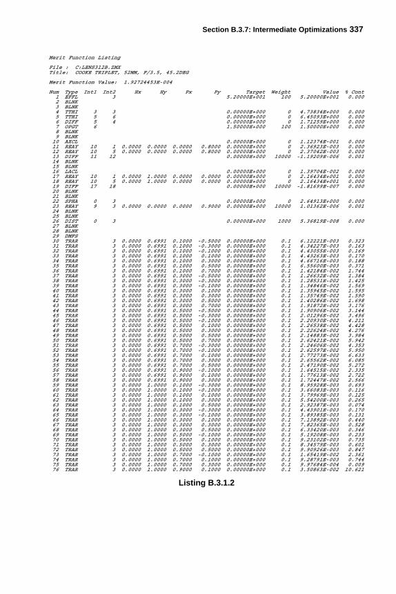
The complete intermediate merit function for the Cooke Triplet is given inListing B.3.1.2. To shorten the listing, the fields have actually been weighted0 0 1 1.

Note that there is a variation to this approach that could have been used. In-stead of controlling spherical aberration with a special operand, you can shrinkthe monochromatic on-axis spot too. To do this, omit the special spherical oper-and (to avoid controlling the same aberration twice), and construct the defaultmerit function with field weights such as 5 1 1 1. The relatively heavy weighton-axis is required because spot size there is relatively small (no off-axis aberra-tions). The heavy weight ensures that the damped least-squares routine paysenough attention.

Note that different optical design programs may handle weights differently.Therefore, it is risky to recommend specific weights for controlling the relativeemphasis of various field positions and wavelengths during optimization. This isespecially true for nonuniform weights. Thus, the weights offered here are given

Section B.3.7: Intermediate Optimizations 337


File : C:LENS312B.ZMXTitle: COOKE TRIPLET, 52MM, F/3.5, 45.2DEG


Num Type Int1 Int2 Hx Hy Px Py Target Weight Value % Cont1 EFFL 3 5.20000E+001 100 5.20000E+001 0.0002 BLNK3 BLNK4 TTHI 3 3 0.00000E+000 0 4.73834E+000 0.0005 TTHI 5 6 0.00000E+000 0 6.45093E+000 0.0006 DIFF 5 4 0.00000E+000 0 1.71259E+000 0.0007 OPGT 6 1.50000E+000 100 1.50000E+000 0.0008 BLNK9 BLNK

10 AXCL 0.00000E+000 0 1.12374E-001 0.00011 REAY 10 1 0.0000 0.0000 0.0000 0.8000 0.00000E+000 0 2.36923E-003 0.00012 REAY 10 5 0.0000 0.0000 0.0000 0.8000 0.00000E+000 0 2.37042E-003 0.00013 DIFF 11 12 0.00000E+000 10000 -1.19209E-006 0.00114 BLNK15 BLNK16 LACL 0.00000E+000 0 1.39704E-002 0.00017 REAY 10 1 0.0000 1.0000 0.0000 0.0000 0.00000E+000 0 2.16434E+001 0.00018 REAY 10 5 0.0000 1.0000 0.0000 0.0000 0.00000E+000 0 2.16434E+001 0.00019 DIFF 17 18 0.00000E+000 10000 -1.81699E-007 0.00020 BLNK21 BLNK22 SPHA 0 3 0.00000E+000 0 2.64913E+000 0.00023 REAY 9 3 0.0000 0.0000 0.0000 0.9000 0.00000E+000 10000 1.01362E-006 0.00124 BLNK25 BLNK26 DIST 0 3 0.00000E+000 1000 5.36819E-008 0.00027 BLNK28 BLNK29 DMFS30 TRAR 3 0.0000 0.6991 0.1000 -0.5000 0.00000E+000 0.1 6.12221E-003 0.32331 TRAR 3 0.0000 0.6991 0.1000 -0.3000 0.00000E+000 0.1 4.34227E-003 0.16332 TRAR 3 0.0000 0.6991 0.1000 -0.1000 0.00000E+000 0.1 4.43055E-003 0.16933 TRAR 3 0.0000 0.6991 0.1000 0.1000 0.00000E+000 0.1 4.43263E-003 0.17034 TRAR 3 0.0000 0.6991 0.1000 0.3000 0.00000E+000 0.1 4.66716E-003 0.18835 TRAR 3 0.0000 0.6991 0.1000 0.5000 0.00000E+000 0.1 6.55600E-003 0.37136 TRAR 3 0.0000 0.6991 0.1000 0.7000 0.00000E+000 0.1 1.42184E-002 1.74437 TRAR 3 0.0000 0.6991 0.3000 -0.5000 0.00000E+000 0.1 1.26632E-002 1.38438 TRAR 3 0.0000 0.6991 0.3000 -0.3000 0.00000E+000 0.1 1.28531E-002 1.42539 TRAR 3 0.0000 0.6991 0.3000 -0.1000 0.00000E+000 0.1 1.34846E-002 1.56940 TRAR 3 0.0000 0.6991 0.3000 0.1000 0.00000E+000 0.1 1.35945E-002 1.59541 TRAR 3 0.0000 0.6991 0.3000 0.3000 0.00000E+000 0.1 1.35749E-002 1.59042 TRAR 3 0.0000 0.6991 0.3000 0.5000 0.00000E+000 0.1 1.40286E-002 1.69843 TRAR 3 0.0000 0.6991 0.3000 0.7000 0.00000E+000 0.1 1.91872E-002 3.17644 TRAR 3 0.0000 0.6991 0.5000 -0.5000 0.00000E+000 0.1 1.90906E-002 3.14445 TRAR 3 0.0000 0.6991 0.5000 -0.3000 0.00000E+000 0.1 2.01296E-002 3.49646 TRAR 3 0.0000 0.6991 0.5000 -0.1000 0.00000E+000 0.1 2.20930E-002 4.21147 TRAR 3 0.0000 0.6991 0.5000 0.1000 0.00000E+000 0.1 2.26538E-002 4.42848 TRAR 3 0.0000 0.6991 0.5000 0.3000 0.00000E+000 0.1 2.22624E-002 4.27649 TRAR 3 0.0000 0.6991 0.5000 0.5000 0.00000E+000 0.1 2.14883E-002 3.98450 TRAR 3 0.0000 0.6991 0.5000 0.7000 0.00000E+000 0.1 2.62421E-002 5.94251 TRAR 3 0.0000 0.6991 0.7000 -0.3000 0.00000E+000 0.1 2.24606E-002 4.35352 TRAR 3 0.0000 0.6991 0.7000 -0.1000 0.00000E+000 0.1 2.62597E-002 5.95053 TRAR 3 0.0000 0.6991 0.7000 0.1000 0.00000E+000 0.1 2.77273E-002 6.63354 TRAR 3 0.0000 0.6991 0.7000 0.3000 0.00000E+000 0.1 2.65562E-002 6.08555 TRAR 3 0.0000 0.6991 0.7000 0.5000 0.00000E+000 0.1 2.47190E-002 5.27256 TRAR 3 0.0000 0.6991 0.9000 -0.1000 0.00000E+000 0.1 1.64515E-002 2.33557 TRAR 3 0.0000 0.6991 0.9000 0.1000 0.00000E+000 0.1 1.77613E-002 2.72258 TRAR 3 0.0000 0.6991 0.9000 0.3000 0.00000E+000 0.1 1.72447E-002 2.56659 TRAR 3 0.0000 1.0000 0.1000 -0.3000 0.00000E+000 0.1 8.95928E-003 0.69360 TRAR 3 0.0000 1.0000 0.1000 -0.1000 0.00000E+000 0.1 3.66083E-003 0.11661 TRAR 3 0.0000 1.0000 0.1000 0.1000 0.00000E+000 0.1 3.79969E-003 0.12562 TRAR 3 0.0000 1.0000 0.1000 0.3000 0.00000E+000 0.1 5.54200E-003 0.26563 TRAR 3 0.0000 1.0000 0.1000 0.5000 0.00000E+000 0.1 2.92387E-003 0.07464 TRAR 3 0.0000 1.0000 0.3000 -0.3000 0.00000E+000 0.1 4.43901E-003 0.17065 TRAR 3 0.0000 1.0000 0.3000 -0.1000 0.00000E+000 0.1 3.89385E-003 0.13166 TRAR 3 0.0000 1.0000 0.3000 0.1000 0.00000E+000 0.1 7.13892E-003 0.44067 TRAR 3 0.0000 1.0000 0.3000 0.3000 0.00000E+000 0.1 7.82365E-003 0.52868 TRAR 3 0.0000 1.0000 0.3000 0.5000 0.00000E+000 0.1 6.33420E-003 0.34669 TRAR 3 0.0000 1.0000 0.5000 -0.1000 0.00000E+000 0.1 5.19208E-003 0.23370 TRAR 3 0.0000 1.0000 0.5000 0.1000 0.00000E+000 0.1 9.23102E-003 0.73571 TRAR 3 0.0000 1.0000 0.5000 0.3000 0.00000E+000 0.1 8.34579E-003 0.60172 TRAR 3 0.0000 1.0000 0.5000 0.5000 0.00000E+000 0.1 9.90926E-003 0.84773 TRAR 3 0.0000 1.0000 0.7000 -0.1000 0.00000E+000 0.1 1.65419E-002 2.36174 TRAR 3 0.0000 1.0000 0.7000 0.1000 0.00000E+000 0.1 9.28791E-003 0.74475 TRAR 3 0.0000 1.0000 0.7000 0.3000 0.00000E+000 0.1 9.97684E-004 0.00976 TRAR 3 0.0000 1.0000 0.9000 0.1000 0.00000E+000 0.1 3.50863E-002 10.621

Listing B.3.1.2


with a caveat. The best advice to the lens designer is to experiment with weightsuntil you get results that you like.

In the design of a Cooke Triplet, you will often find two possible solutions;that is, two different local minima of the merit function. The first solution has thelarger airspace between the front and middle elements; the second solution has thelarger airspace between the middle and rear elements. As mentioned earlier, bettersymmetry about the stop is achieved if the rear airspace is the larger one. Thismore symmetrical configuration causes the off-axis beams to be more centeredabout their chief rays, which is better when stopping down the lens. To shepherdthe design in this direction, a constraint is added to the intermediate merit func-tion that keeps the rear airspace (glass-to-glass) somewhat larger than the frontairspace.

After optimizing with the airspace constraint, look at the merit function tosee if it was invoked. It may have been unused. If it was used, try removing it (per-haps by setting its weight to zero) and optimize again. The lens will then find itsown best airspaces. However, do not be surprised if the negative element ends upnearly in the middle between the two positive elements, or if you occasionallyhave to leave in the constraint.

After each optimization run, the system parameters (curvatures and airspac-es) will have changed to a greater or lesser extent, thereby also changing the sizeand shape of the vignetted off-axis pupils. To accommodate these changes, re-build the default merit function to update the set of unvignetted rays, and then re-optimize. Iterate as needed. In addition, the lens designer is also often required tomanually readjust the diameters of the hard apertures to maintain the desiredamount of vignetting. After any such change, again rebuild the default merit func-tion and reoptimize.

The last step in the intermediate optimizations is finding the best flint glasstype. To do this, repeat the intermediate optimization with several likely glasscombinations. The process is described in an earlier section. The result for thepresent Cooke Triplet is that Schott SF53 flint glass (nd of 1.728, Vd of 28.7) isthe best match for Schott LaFN21 crown glass (nd of 1.788, Vd of 47.5).

B.3.2 Final Optimizations Using Spot Size

The intermediate solution for the Cooke Triplet is actually quite close to thefinal solution. The final solution is a refinement, which is normally accomplishedin two stages. The first stage shrinks polychromatic spots on the image surface.The second stage minimizes polychromatic OPD errors in the exit pupil. The de-signer then compares the two solutions and chooses the better one for the givenapplication. If MTF is the image criterion, then the OPD solution is usually, butnot always, preferable.

There are two ways to do the final spot optimization. The first way uses a

Section B.3.2: Final Optimizations Using Spot Size 339

merit function that shrinks polychromatic spot sizes for all field positions and allwavelengths while continuing to correct distortion and focal length with specialoperands. Note that longitudinal and lateral color are not individually corrected;the polychromatic spot optimization includes the chromatic aberrations. Thus,when constructing the default merit function, weight the four fields equally; thatis, 1 1 1 1, at least initially. Also weight the five wavelengths equally; that is,1 1 1 1. As an alternative, you might do as just described plus still continue to ex-actly correct longitudinal color with a special operand to ensure a specific colorcurve.

The second way is very similar except that the on-axis aberrations (longitu-dinal color and spherical aberration) are corrected with special operands, and thedefault merit function shrinks polychromatic spots only off-axis. Again, distor-tion and focal length are specially corrected. When constructing the default meritfunction, the on-axis spot is turned off by weighting this field position zero; thatis, field weights are 0 1 1 1 (at least initially). The polychromatic wavelengthweights are again 1 1 1 1 1. In the present Cooke Triplet example, this secondmethod has been adopted for constructing the merit function.

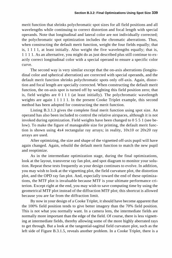
Listing B.3.1.3 gives the complete final merit function using spot size. Anoperand has also been included to control the relative airspaces, although it is notinvoked during optimization. Field weights have been changed to 0 5 5 1 (see be-low). To make the figure of manageable size for printing, the default merit func-tion is shown using 4x4 rectangular ray arrays; in reality, 10x10 or 20x20 rayarrays are used.

After optimizing, the size and shape of the vignetted off-axis pupil will haveagain changed. Again, rebuild the default merit function to match the new pupiland reoptimize.

As in the intermediate optimization stage, during the final optimizations,look at the layout, transverse ray fan plot, and spot diagram to monitor your solu-tion. Repeat these tests frequently as your design continues to evolve. In addition,you may wish to look at the vignetting plot, the field curvature plot, the distortionplot, and the OPD ray fan plot. And, especially toward the end of these optimiza-tions, the MTF plot is invaluable because MTF is your ultimate performance cri-terion. Except right at the end, you may wish to save computing time by using thegeometrical MTF plot instead of the diffraction MTF plot; this shortcut is allowedbecause you are far from the diffraction limit.

By now in your design of a Cooke Triplet, it should have become apparent thatthe 100% field position tends to give better imagery than the 70% field position.This is not what you normally want. In a camera lens, the intermediate fields arenormally more important than the edge of the field. Of course, there is less vignett-ing at intermediate fields, thereby allowing some of the more highly aberrated raysto get through. But a look at the tangential-sagittal field curvature plot, such as theleft side of Figure B.3.1.5, reveals another problem. In a Cooke Triplet, there is a





Num Type Int1 Int2 Hx Hy Px Py Target Weight Value % Cont1 EFFL 3 5.20000E+001 1000 5.20000E+001 0.0002 BLNK3 BLNK4 TTHI 3 3 0.00000E+000 0 4.32187E+000 0.0005 TTHI 5 6 0.00000E+000 0 6.85434E+000 0.0006 DIFF 5 4 0.00000E+000 0 2.53247E+000 0.0007 OPGT 6 1.50000E+000 1000 1.50000E+000 0.0008 BLNK9 BLNK

10 AXCL 0.00000E+000 0 1.11785E-001 0.00011 REAY 10 1 0.0000 0.0000 0.0000 0.8000 0.00000E+000 0 2.26244E-003 0.00012 REAY 10 5 0.0000 0.0000 0.0000 0.8000 0.00000E+000 0 2.33925E-003 0.00013 DIFF 11 12 0.00000E+000 10000 -7.68052E-005 0.95914 BLNK15 BLNK16 SPHA 0 3 0.00000E+000 0 2.69377E+000 0.00017 REAY 9 3 0.0000 0.0000 0.0000 0.9000 0.00000E+000 10000 1.10586E-004 1.98918 BLNK19 BLNK20 DIST 0 3 0.00000E+000 1000 2.01569E-006 0.00021 BLNK22 BLNK23 DMFS24 TRAR 1 0.0000 0.3982 0.2500 -0.7500 0.00000E+000 0.5 1.13189E-002 1.04225 TRAR 1 0.0000 0.3982 0.2500 -0.2500 0.00000E+000 0.5 6.13682E-003 0.30626 TRAR 1 0.0000 0.3982 0.2500 0.2500 0.00000E+000 0.5 6.79766E-003 0.37627 TRAR 1 0.0000 0.3982 0.2500 0.7500 0.00000E+000 0.5 4.29339E-003 0.15028 TRAR 1 0.0000 0.3982 0.7500 -0.2500 0.00000E+000 0.5 8.61819E-003 0.60429 TRAR 1 0.0000 0.3982 0.7500 0.2500 0.00000E+000 0.5 1.09141E-002 0.96930 TRAR 2 0.0000 0.3982 0.2500 -0.7500 0.00000E+000 0.5 4.39938E-003 0.15731 TRAR 2 0.0000 0.3982 0.2500 -0.2500 0.00000E+000 0.5 7.75161E-003 0.48932 TRAR 2 0.0000 0.3982 0.2500 0.2500 0.00000E+000 0.5 7.13903E-003 0.41433 TRAR 2 0.0000 0.3982 0.2500 0.7500 0.00000E+000 0.5 8.18535E-003 0.54534 TRAR 2 0.0000 0.3982 0.7500 -0.2500 0.00000E+000 0.5 1.46952E-002 1.75635 TRAR 2 0.0000 0.3982 0.7500 0.2500 0.00000E+000 0.5 1.75552E-002 2.50636 TRAR 3 0.0000 0.3982 0.2500 -0.7500 0.00000E+000 0.5 4.13661E-003 0.13937 TRAR 3 0.0000 0.3982 0.2500 -0.2500 0.00000E+000 0.5 6.83198E-003 0.38038 TRAR 3 0.0000 0.3982 0.2500 0.2500 0.00000E+000 0.5 5.77825E-003 0.27239 TRAR 3 0.0000 0.3982 0.2500 0.7500 0.00000E+000 0.5 7.22030E-003 0.42440 TRAR 3 0.0000 0.3982 0.7500 -0.2500 0.00000E+000 0.5 1.48809E-002 1.80141 TRAR 3 0.0000 0.3982 0.7500 0.2500 0.00000E+000 0.5 1.74078E-002 2.46442 TRAR 4 0.0000 0.3982 0.2500 -0.7500 0.00000E+000 0.5 5.52951E-003 0.24943 TRAR 4 0.0000 0.3982 0.2500 -0.2500 0.00000E+000 0.5 4.88180E-003 0.19444 TRAR 4 0.0000 0.3982 0.2500 0.2500 0.00000E+000 0.5 4.11031E-003 0.13745 TRAR 4 0.0000 0.3982 0.2500 0.7500 0.00000E+000 0.5 5.03739E-003 0.20646 TRAR 4 0.0000 0.3982 0.7500 -0.2500 0.00000E+000 0.5 1.21386E-002 1.19847 TRAR 4 0.0000 0.3982 0.7500 0.2500 0.00000E+000 0.5 1.44850E-002 1.70648 TRAR 5 0.0000 0.3982 0.2500 -0.7500 0.00000E+000 0.5 9.21534E-003 0.69149 TRAR 5 0.0000 0.3982 0.2500 -0.2500 0.00000E+000 0.5 3.01616E-003 0.07450 TRAR 5 0.0000 0.3982 0.2500 0.2500 0.00000E+000 0.5 3.22798E-003 0.08551 TRAR 5 0.0000 0.3982 0.2500 0.7500 0.00000E+000 0.5 5.54136E-003 0.25052 TRAR 5 0.0000 0.3982 0.7500 -0.2500 0.00000E+000 0.5 8.23579E-003 0.55253 TRAR 5 0.0000 0.3982 0.7500 0.2500 0.00000E+000 0.5 1.04533E-002 0.88954 TRAR 1 0.0000 0.6991 0.2500 -0.2500 0.00000E+000 0.5 1.18736E-002 1.14655 TRAR 1 0.0000 0.6991 0.2500 0.2500 0.00000E+000 0.5 1.22854E-002 1.22756 TRAR 1 0.0000 0.6991 0.2500 0.7500 0.00000E+000 0.5 1.48341E-002 1.78957 TRAR 1 0.0000 0.6991 0.7500 -0.2500 0.00000E+000 0.5 1.72910E-002 2.43158 TRAR 1 0.0000 0.6991 0.7500 0.2500 0.00000E+000 0.5 2.11634E-002 3.64259 TRAR 2 0.0000 0.6991 0.2500 -0.2500 0.00000E+000 0.5 1.34572E-002 1.47360 TRAR 2 0.0000 0.6991 0.2500 0.2500 0.00000E+000 0.5 1.23649E-002 1.24361 TRAR 2 0.0000 0.6991 0.2500 0.7500 0.00000E+000 0.5 1.53093E-002 1.90662 TRAR 2 0.0000 0.6991 0.7500 -0.2500 0.00000E+000 0.5 2.26614E-002 4.17663 TRAR 2 0.0000 0.6991 0.7500 0.2500 0.00000E+000 0.5 2.82597E-002 6.49464 TRAR 3 0.0000 0.6991 0.2500 -0.2500 0.00000E+000 0.5 1.24155E-002 1.25365 TRAR 3 0.0000 0.6991 0.2500 0.2500 0.00000E+000 0.5 1.12590E-002 1.03166 TRAR 3 0.0000 0.6991 0.2500 0.7500 0.00000E+000 0.5 1.80932E-002 2.66267 TRAR 3 0.0000 0.6991 0.7500 -0.2500 0.00000E+000 0.5 2.30272E-002 4.31268 TRAR 3 0.0000 0.6991 0.7500 0.2500 0.00000E+000 0.5 2.85360E-002 6.62269 TRAR 4 0.0000 0.6991 0.2500 -0.2500 0.00000E+000 0.5 1.05241E-002 0.90170 TRAR 4 0.0000 0.6991 0.2500 0.2500 0.00000E+000 0.5 9.94036E-003 0.80371 TRAR 4 0.0000 0.6991 0.2500 0.7500 0.00000E+000 0.5 2.20493E-002 3.95372 TRAR 4 0.0000 0.6991 0.7500 -0.2500 0.00000E+000 0.5 2.09049E-002 3.55473 TRAR 4 0.0000 0.6991 0.7500 0.2500 0.00000E+000 0.5 2.60342E-002 5.51274 TRAR 5 0.0000 0.6991 0.2500 -0.2500 0.00000E+000 0.5 8.88009E-003 0.64175 TRAR 5 0.0000 0.6991 0.2500 0.2500 0.00000E+000 0.5 8.85322E-003 0.63776 TRAR 5 0.0000 0.6991 0.2500 0.7500 0.00000E+000 0.5 2.67318E-002 5.81177 TRAR 5 0.0000 0.6991 0.7500 -0.2500 0.00000E+000 0.5 1.80876E-002 2.66078 TRAR 5 0.0000 0.6991 0.7500 0.2500 0.00000E+000 0.5 2.24098E-002 4.08479 TRAR 1 0.0000 1.0000 0.2500 -0.2500 0.00000E+000 0.1 3.54277E-002 2.04180 TRAR 1 0.0000 1.0000 0.2500 0.2500 0.00000E+000 0.1 1.64360E-002 0.43981 TRAR 1 0.0000 1.0000 0.7500 0.2500 0.00000E+000 0.1 1.29293E-002 0.27282 TRAR 2 0.0000 1.0000 0.2500 -0.2500 0.00000E+000 0.1 2.87876E-002 1.34883 TRAR 2 0.0000 1.0000 0.2500 0.2500 0.00000E+000 0.1 1.25153E-002 0.25584 TRAR 2 0.0000 1.0000 0.7500 0.2500 0.00000E+000 0.1 4.61541E-003 0.03585 TRAR 3 0.0000 1.0000 0.2500 -0.2500 0.00000E+000 0.1 2.09629E-002 0.71586 TRAR 3 0.0000 1.0000 0.2500 0.2500 0.00000E+000 0.1 9.28730E-003 0.14087 TRAR 3 0.0000 1.0000 0.7500 0.2500 0.00000E+000 0.1 4.84668E-003 0.03888 TRAR 4 0.0000 1.0000 0.2500 -0.2500 0.00000E+000 0.1 1.32269E-002 0.28589 TRAR 4 0.0000 1.0000 0.2500 0.2500 0.00000E+000 0.1 6.43729E-003 0.06790 TRAR 4 0.0000 1.0000 0.7500 0.2500 0.00000E+000 0.1 8.04721E-003 0.10591 TRAR 5 0.0000 1.0000 0.2500 -0.2500 0.00000E+000 0.1 5.90391E-003 0.05792 TRAR 5 0.0000 1.0000 0.2500 0.2500 0.00000E+000 0.1 3.94329E-003 0.02593 TRAR 5 0.0000 1.0000 0.7500 0.2500 0.00000E+000 0.1 1.22290E-002 0.243

Listing B.3.1.3


large difference between the tangential and sagittal curves at intermediate fields,but the curves cross near the field edge. Thus, at intermediate field zones you get alot of astigmatism, but astigmatism goes to zero near the field edge.

This astigmatic behavior is the result of the interaction of relatively largeamounts of third- and fifth-order astigmatism (seventh is negligible). The sum ofthe third- and fifth-orders is zero at the field angle where the curves cross. Unfor-tunately, at other field angles the sum may not be small. Third-order predominatesinside the crossing, and fifth-order predominates outside the crossing. The prob-lem is analogous to zonal spherical aberration, except that the effect is in the field,not the pupil. Significant residual field-zonal astigmatism is part of the inherentnature of a Cooke Triplet.

The use of high-index glasses generally reduces this astigmatism and ishighly recommended. The only other thing you can do is tell the computer tochange its priorities and emphasize the intermediate fields at the expense of thefield edge; that is, you increase the relative weights on the two intermediate fieldsduring optimization. This moves the field angle for zero astigmatism inward. Un-fortunately, astigmatism increases very rapidly for field angles outside the tan-gential-sagittal crossing. You must therefore be very careful to avoid overdoingthis brute force tactic. Also, the computer has other aberrations to worry about be-sides astigmatism, which is why the crossing initially fell so far out. A reasonablesolution is obtained if the default part of the merit function is rebuilt with the fieldweights changed from 0 1 1 1 to 0 5 5 1 (while continuing to separately correctthe on-axis field with special operands). The intermediate fields get better whilethe edge of the field gets worse.

This illustrates a recurrent situation in lens design. A given lens configura-tion has only a certain ability to control aberrations. If you take a previously op-timized lens and reoptimize it to make one thing better, something else must getworse. There is an adage that says that the process of reoptimizing a lens is likesqueezing on a water balloon. If you squeeze in one place, it pops out somewhereelse.

Figure B.3.1.1 shows the layout of the Cooke Triplet as optimized by cor-recting focal length, distortion, and special on-axis operands; by shrinking poly-chromatic off-axis spots; and by emphasizing the intermediate fields. Forincreased clarity, the beams for only two fields have been drawn, the on-axis fieldand the extreme off-axis field. Note the mechanical vignetting of the off-axisbeam by the front and rear outside lens surfaces. Note too that what appears to bethe off-axis chief ray does not go through the center of the stop. Actually, the rayin question is not the chief ray, but is merely the middle ray of the ray bundle. Thetrue chief ray always goes exactly through the center of the stop, by definition.

Figure B.3.1.3 is the vignetting diagram showing the fraction of unvignettedrays as a function of field angle. This plot confirms that vignetting is well-be-haved and is about 50% at the edge of the field.


Figure B.3.1.4 is the transverse ray fan plot. Note the well-behaved on-axiscurves. For the three off-axis fields, note how the slopes of the tangential and sag-ittal curves are different at the origin, indicating astigmatism. Note too the ob-lique spherical aberration in the off-axis fields. Finally, note that the chromaticaberrations are relatively small compared to the monochromatic aberrations.

On the left side of Figure B.3.1.5 is the field curvature plot. Note the cross-ing of the tangential and sagittal curves near the field edge and the large astigmat-ic difference at intermediate field angles. On the right side of Figure B.3.1.5 is thepercent distortion plot. Distortion has been corrected to zero at the field edge, butnote the higher-order distortion residuals at intermediate field angles. These re-siduals are tiny and totally negligible for most purposes.

Figure B.3.1.6 is the polychromatic spot diagram. Note the different appear-ance of the spots. The spot for the 70% field is spread horizontally by tangentialastigmatism, and the spot for the field edge is spread vertically by sagittal (radial)astigmatism. However, these images are not purely astigmatic because other ab-errations are complicating the situation.

Figure B.3.1.7 is the matrix spot diagram. Note that the spots vary stronglywith field but only moderately with wavelength.

Figure B.3.1.8 is the OPD ray fan plot. Note the scale: several waves. Clear-

Figure B.3.1.3


Figure B.3.1.4

Figure B.3.1.5


ly, this lens is aberration limited, not diffraction limited. Even on-axis, this lensdoes not satisfy the Rayleigh quarter-wave rule. But this performance level is nor-mal for this type of lens and is no cause for concern. At f/3.5 and for a wavelengthof 0.55 μm, the diameter of the Airy disk is only 4.7 μm and the diffraction MTFcutoff is 520 cycles/mm. These values are much finer than most films can resolve.In fact, very few camera lenses are diffraction limited when used wide open, andmost of these are slow, long-focus lenses.

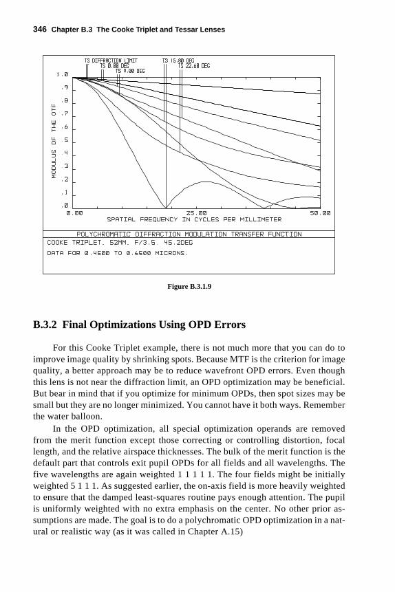
Figure B.3.1.9 is the diffraction MTF plot. Even with increased weight onthe intermediate fields during optimization, the sagittal MTF at the 70% field isvery poor. Still heavier weights are not recommended; the spot size at the edge ofthe field would explode without much benefit to the intermediate fields. Note thespurious resolution. This artifact of the periodic nature of a pure spatial frequencyis of no help for real images; modulations beyond the first zero must be ignoredwhen evaluating lens performance.

Listing B.3.1.4 is the optical prescription for the spot size optimized CookeTriplet. From this listing, you could build the lens. However, for a practical cam-era lens intended for use with films having a resolving capability in excess of50 cycles/mm, this design for the Cooke Triplet is probably unacceptable, at leastby modern standards based on MTF.

Figure B.3.1.6


Figure B.3.1.7

Figure B.3.1.8


B.3.2 Final Optimizations Using OPD Errors

For this Cooke Triplet example, there is not much more that you can do toimprove image quality by shrinking spots. Because MTF is the criterion for imagequality, a better approach may be to reduce wavefront OPD errors. Even thoughthis lens is not near the diffraction limit, an OPD optimization may be beneficial.But bear in mind that if you optimize for minimum OPDs, then spot sizes may besmall but they are no longer minimized. You cannot have it both ways. Rememberthe water balloon.

In the OPD optimization, all special optimization operands are removedfrom the merit function except those correcting or controlling distortion, focallength, and the relative airspace thicknesses. The bulk of the merit function is thedefault part that controls exit pupil OPDs for all fields and all wavelengths. Thefive wavelengths are again weighted 1 1 1 1 1. The four fields might be initiallyweighted 5 1 1 1. As suggested earlier, the on-axis field is more heavily weightedto ensure that the damped least-squares routine pays enough attention. The pupilis uniformly weighted with no extra emphasis on the center. No other prior as-sumptions are made. The goal is to do a polychromatic OPD optimization in a nat-ural or realistic way (as it was called in Chapter A.15)

Figure B.3.1.9

Section B.3.2: Final Optimizations Using OPD Errors 347

Listing B.3.2.1 is the complete final merit function for an OPD optimization.The field weights have been changed to 4 3 2 1 (see below). Again for practicalreasons, 4x4 ray arrays are shown, although 10x10 or 20x20 arrays are actuallyused when optimizing. Note that the control on the relative airspace thicknessesis not invoked.

After optimizing with OPDs, the lens elements will have shifted by someamount relative to their positions for the minimum spot size solution. Thus, afterthe first OPD optimization, the vignetting will have changed and you must rebuildthe default merit function and reoptimize. In addition, you may wish to fine tunethe vignetting curve to give a specific throughput value at the edge of the field.This is done by slightly changing the vignetting apertures, again rebuilding themerit function, and again reoptimizing.

Next, do the usual layout, transverse ray fan plot, and spot diagram as sanitychecks. Then do an OPD ray fan plot to check your OPD optimization. Finally,do the crucial MTF plot. As with a spot size optimization, an OPD optimizationwith uniform weights on the off-axis fields yields poorer performance for the in-termediate fields than for the extreme field. The (partial) remedy once again is toincrease the weights on the intermediate fields. Try different sets of weights, re-optimize for each set, and compare the MTF curves. Select the weights that givethe best overall compromise. In the present case, field weights of 4 3 2 1 are foundto work well.

Recall that in the present example, vignetting is handled during optimization

Listing B.3.1.4

System/Prescription Data


GENERAL LENS DATA:

Surfaces : 10Stop : 6System Aperture :Entrance Pupil DiameterRay aiming : OnX Pupil shift : 0Y Pupil shift : 0Z Pupil shift : 0Apodization :Uniform, factor = 0.000000Eff. Focal Len. : 52 (in air)Eff. Focal Len. : 52 (in image space)Total Track : 67.753Image Space F/# : 3.49933Para. Wrkng F/# : 3.49933Working F/# : 3.55795Obj. Space N.A. : 7.43e-010Stop Radius : 5.73158Parax. Ima. Hgt.: 21.6455Parax. Mag. : 0Entr. Pup. Dia. : 14.86Entr. Pup. Pos. : 19.9395Exit Pupil Dia. : 14.1746Exit Pupil Pos. : -49.6015Field Type : Angle in degreesMaximum Field : 22.6Primary Wave : 0.550000Lens Units : MillimetersAngular Mag. : 1.04835

Fields : 4Field Type: Angle in degrees# X-Value Y-Value Weight1 0.000000 0.000000 0.0000002 0.000000 9.000000 5.0000003 0.000000 15.800000 5.0000004 0.000000 22.600000 1.000000


by deleting the vignetted rays from a set of incident rays. This deletion has thesubtle side effect of reducing the working weights on the fields with more vignett-ing and fewer transmitted rays. Fewer rays yield fewer optimization operands.Fewer operands make less of a contribution to the damped least-squares solution.

Listing B.3.1.4 (continued)

Vignetting Factors# VDX VDY VCX VCY1 0.000000 0.000000 0.000000 0.0000002 0.000000 0.000000 0.000000 0.0000003 0.000000 0.000000 0.000000 0.0000004 0.000000 0.000000 0.000000 0.000000

Wavelengths : 5Units: Microns# Value Weight1 0.450000 1.0000002 0.500000 1.0000003 0.550000 1.0000004 0.600000 1.0000005 0.650000 1.000000

SURFACE DATA SUMMARY:

Surf Type Radius Thickness Glass Diameter ConicOBJ STANDARD Infinity Infinity 0 0

1 STANDARD Infinity 7 33.36006 02 STANDARD 21.74267 3.5 LAFN21 17 03 STANDARD 400.8834 4.321867 17 04 STANDARD -43.54159 1.5 SF53 13 05 STANDARD 20.87459 2 12 0

STO STANDARD Infinity 4.854339 11.46317 07 STANDARD 165.5048 3 LAFN21 15 08 STANDARD -30.5771 41.57679 15 09 STANDARD Infinity 0 43.61234 0

IMA STANDARD Infinity 0 43.61234 0

SURFACE DATA DETAIL:

Surface OBJ : STANDARDSurface 1 : STANDARDSurface 2 : STANDARDAperture : Circular ApertureMinimum Radius : 0Maximum Radius : 8.5Surface 3 : STANDARDSurface 4 : STANDARDSurface 5 : STANDARDSurface STO : STANDARDSurface 7 : STANDARDSurface 8 : STANDARDAperture : Circular ApertureMinimum Radius : 0Maximum Radius : 7.5Surface 9 : STANDARDSurface IMA : STANDARD

SOLVE AND VARIABLE DATA:

Curvature of 2 : VariableSemi Diam 2 : FixedCurvature of 3 : VariableThickness of 3 : VariableSemi Diam 3 : FixedCurvature of 4 : VariableSemi Diam 4 : FixedCurvature of 5 : VariableSemi Diam 5 : FixedThickness of 6 : VariableCurvature of 7 : VariableSemi Diam 7 : FixedCurvature of 8 : VariableThickness of 8 : Solve, marginal ray height = 0.00000Semi Diam 8 : Fixed

INDEX OF REFRACTION DATA:

Surf Glass 0.450000 0.500000 0.550000 0.600000 0.6500000 1.00000000 1.00000000 1.00000000 1.00000000 1.000000001 1.00000000 1.00000000 1.00000000 1.00000000 1.000000002 LAFN21 1.80620521 1.79788762 1.79184804 1.78728036 1.783707733 1.00000000 1.00000000 1.00000000 1.00000000 1.000000004 SF53 1.75665336 1.74309602 1.73366378 1.72676633 1.721527895 1.00000000 1.00000000 1.00000000 1.00000000 1.000000006 1.00000000 1.00000000 1.00000000 1.00000000 1.000000007 LAFN21 1.80620521 1.79788762 1.79184804 1.78728036 1.783707738 1.00000000 1.00000000 1.00000000 1.00000000 1.000000009 1.00000000 1.00000000 1.00000000 1.00000000 1.00000000

10 1.00000000 1.00000000 1.00000000 1.00000000 1.00000000

ELEMENT VOLUME DATA:

Units are cubic cm.Values are only accurate for plane and spherical surfaces.Element surf 2 to 3 volume : 0.610995Element surf 4 to 5 volume : 0.269441Element surf 7 to 8 volume : 0.433018





Num Type Int1 Int2 Hx Hy Px Py Target Weight Value % Cont1 EFFL 3 5.20000E+001 1e+005 5.20001E+001 0.0052 BLNK3 BLNK4 TTHI 3 3 0.00000E+000 0 4.01727E+000 0.0005 TTHI 5 6 0.00000E+000 0 7.19832E+000 0.0006 DIFF 5 4 0.00000E+000 0 3.18105E+000 0.0007 OPGT 6 1.50000E+000 1e+005 1.50000E+000 0.0008 BLNK9 BLNK

10 DIST 0 3 0.00000E+000 1e+005 7.33768E-006 0.00011 BLNK12 BLNK13 DMFS14 OPDC 1 0.0000 0.0000 0.2500 0.2500 0.00000E+000 0.8 8.28033E-003 0.00015 OPDC 1 0.0000 0.0000 0.2500 0.7500 0.00000E+000 0.8 -1.93433E-001 0.17716 OPDC 1 0.0000 0.0000 0.7500 0.2500 0.00000E+000 0.8 -1.93433E-001 0.17717 OPDC 2 0.0000 0.0000 0.2500 0.2500 0.00000E+000 0.8 8.69492E-002 0.03618 OPDC 2 0.0000 0.0000 0.2500 0.7500 0.00000E+000 0.8 4.49848E-001 0.95719 OPDC 2 0.0000 0.0000 0.7500 0.2500 0.00000E+000 0.8 4.49848E-001 0.95720 OPDC 3 0.0000 0.0000 0.2500 0.2500 0.00000E+000 0.8 3.10335E-002 0.00521 OPDC 3 0.0000 0.0000 0.2500 0.7500 0.00000E+000 0.8 3.05747E-001 0.44222 OPDC 3 0.0000 0.0000 0.7500 0.2500 0.00000E+000 0.8 3.05747E-001 0.44223 OPDC 4 0.0000 0.0000 0.2500 0.2500 0.00000E+000 0.8 -5.79185E-002 0.01624 OPDC 4 0.0000 0.0000 0.2500 0.7500 0.00000E+000 0.8 -6.32398E-002 0.01925 OPDC 4 0.0000 0.0000 0.7500 0.2500 0.00000E+000 0.8 -6.32398E-002 0.01926 OPDC 5 0.0000 0.0000 0.2500 0.2500 0.00000E+000 0.8 -1.48682E-001 0.10527 OPDC 5 0.0000 0.0000 0.2500 0.7500 0.00000E+000 0.8 -4.74652E-001 1.06628 OPDC 5 0.0000 0.0000 0.7500 0.2500 0.00000E+000 0.8 -4.74652E-001 1.06629 OPDC 1 0.0000 0.3982 0.2500 -0.7500 0.00000E+000 0.3 -1.07468E+000 2.04830 OPDC 1 0.0000 0.3982 0.2500 -0.2500 0.00000E+000 0.3 8.80501E-002 0.01431 OPDC 1 0.0000 0.3982 0.2500 0.2500 0.00000E+000 0.3 2.50417E-001 0.11132 OPDC 1 0.0000 0.3982 0.2500 0.7500 0.00000E+000 0.3 9.56563E-003 0.00033 OPDC 1 0.0000 0.3982 0.7500 -0.2500 0.00000E+000 0.3 7.60901E-001 1.02734 OPDC 1 0.0000 0.3982 0.7500 0.2500 0.00000E+000 0.3 1.18858E+000 2.50635 OPDC 2 0.0000 0.3982 0.2500 -0.7500 0.00000E+000 0.3 -1.67402E-001 0.05036 OPDC 2 0.0000 0.3982 0.2500 -0.2500 0.00000E+000 0.3 2.29260E-001 0.09337 OPDC 2 0.0000 0.3982 0.2500 0.2500 0.00000E+000 0.3 2.18183E-001 0.08438 OPDC 2 0.0000 0.3982 0.2500 0.7500 0.00000E+000 0.3 3.01055E-001 0.16139 OPDC 2 0.0000 0.3982 0.7500 -0.2500 0.00000E+000 0.3 1.39278E+000 3.44140 OPDC 2 0.0000 0.3982 0.7500 0.2500 0.00000E+000 0.3 1.60406E+000 4.56441 OPDC 3 0.0000 0.3982 0.2500 -0.7500 0.00000E+000 0.3 -2.28682E-001 0.09342 OPDC 3 0.0000 0.3982 0.2500 -0.2500 0.00000E+000 0.3 1.71230E-001 0.05243 OPDC 3 0.0000 0.3982 0.2500 0.2500 0.00000E+000 0.3 1.31326E-001 0.03144 OPDC 3 0.0000 0.3982 0.2500 0.7500 0.00000E+000 0.3 6.06463E-002 0.00745 OPDC 3 0.0000 0.3982 0.7500 -0.2500 0.00000E+000 0.3 1.18771E+000 2.50246 OPDC 3 0.0000 0.3982 0.7500 0.2500 0.00000E+000 0.3 1.33141E+000 3.14447 OPDC 4 0.0000 0.3982 0.2500 -0.7500 0.00000E+000 0.3 -5.82113E-001 0.60148 OPDC 4 0.0000 0.3982 0.2500 -0.2500 0.00000E+000 0.3 5.92456E-002 0.00649 OPDC 4 0.0000 0.3982 0.2500 0.2500 0.00000E+000 0.3 4.09036E-002 0.00350 OPDC 4 0.0000 0.3982 0.2500 0.7500 0.00000E+000 0.3 -3.06883E-001 0.16751 OPDC 4 0.0000 0.3982 0.7500 -0.2500 0.00000E+000 0.3 7.46006E-001 0.98752 OPDC 4 0.0000 0.3982 0.7500 0.2500 0.00000E+000 0.3 8.79151E-001 1.37153 OPDC 5 0.0000 0.3982 0.2500 -0.7500 0.00000E+000 0.3 -1.00425E+000 1.78954 OPDC 5 0.0000 0.3982 0.2500 -0.2500 0.00000E+000 0.3 -6.03986E-002 0.00655 OPDC 5 0.0000 0.3982 0.2500 0.2500 0.00000E+000 0.3 -4.01545E-002 0.00356 OPDC 5 0.0000 0.3982 0.2500 0.7500 0.00000E+000 0.3 -6.78202E-001 0.81657 OPDC 5 0.0000 0.3982 0.7500 -0.2500 0.00000E+000 0.3 2.62630E-001 0.12258 OPDC 5 0.0000 0.3982 0.7500 0.2500 0.00000E+000 0.3 4.08174E-001 0.29659 OPDC 1 0.0000 0.6991 0.2500 -0.2500 0.00000E+000 0.2 2.91949E-001 0.10160 OPDC 1 0.0000 0.6991 0.2500 0.2500 0.00000E+000 0.2 3.83947E-001 0.17461 OPDC 1 0.0000 0.6991 0.2500 0.7500 0.00000E+000 0.2 -1.75633E+000 3.64862 OPDC 1 0.0000 0.6991 0.7500 -0.2500 0.00000E+000 0.2 1.60934E+000 3.06363 OPDC 1 0.0000 0.6991 0.7500 0.2500 0.00000E+000 0.2 1.95819E+000 4.53464 OPDC 2 0.0000 0.6991 0.2500 -0.2500 0.00000E+000 0.2 4.02041E-001 0.19165 OPDC 2 0.0000 0.6991 0.2500 0.2500 0.00000E+000 0.2 2.71910E-001 0.08766 OPDC 2 0.0000 0.6991 0.2500 0.7500 0.00000E+000 0.2 -1.67794E+000 3.32967 OPDC 2 0.0000 0.6991 0.7500 -0.2500 0.00000E+000 0.2 2.15371E+000 5.48568 OPDC 2 0.0000 0.6991 0.7500 0.2500 0.00000E+000 0.2 2.24437E+000 5.95669 OPDC 3 0.0000 0.6991 0.2500 -0.2500 0.00000E+000 0.2 2.97159E-001 0.10470 OPDC 3 0.0000 0.6991 0.2500 0.2500 0.00000E+000 0.2 1.67794E-001 0.03371 OPDC 3 0.0000 0.6991 0.2500 0.7500 0.00000E+000 0.2 -1.89446E+000 4.24472 OPDC 3 0.0000 0.6991 0.7500 -0.2500 0.00000E+000 0.2 1.86086E+000 4.09573 OPDC 3 0.0000 0.6991 0.7500 0.2500 0.00000E+000 0.2 1.91078E+000 4.31774 OPDC 4 0.0000 0.6991 0.2500 -0.2500 0.00000E+000 0.2 1.40219E-001 0.02375 OPDC 4 0.0000 0.6991 0.2500 0.2500 0.00000E+000 0.2 8.22733E-002 0.00876 OPDC 4 0.0000 0.6991 0.2500 0.7500 0.00000E+000 0.2 -2.15451E+000 5.48977 OPDC 4 0.0000 0.6991 0.7500 -0.2500 0.00000E+000 0.2 1.34077E+000 2.12678 OPDC 4 0.0000 0.6991 0.7500 0.2500 0.00000E+000 0.2 1.42478E+000 2.40079 OPDC 5 0.0000 0.6991 0.2500 -0.2500 0.00000E+000 0.2 -1.87010E-002 0.00080 OPDC 5 0.0000 0.6991 0.2500 0.2500 0.00000E+000 0.2 1.39299E-002 0.00081 OPDC 5 0.0000 0.6991 0.2500 0.7500 0.00000E+000 0.2 -2.39172E+000 6.76482 OPDC 5 0.0000 0.6991 0.7500 -0.2500 0.00000E+000 0.2 7.89234E-001 0.73783 OPDC 5 0.0000 0.6991 0.7500 0.2500 0.00000E+000 0.2 9.32214E-001 1.02884 OPDC 1 0.0000 1.0000 0.2500 -0.2500 0.00000E+000 0.1 1.73150E+000 1.77385 OPDC 1 0.0000 1.0000 0.2500 0.2500 0.00000E+000 0.1 3.86223E-001 0.08886 OPDC 1 0.0000 1.0000 0.7500 0.2500 0.00000E+000 0.1 -2.10541E+000 2.62187 OPDC 2 0.0000 1.0000 0.2500 -0.2500 0.00000E+000 0.1 1.24723E+000 0.92088 OPDC 2 0.0000 1.0000 0.2500 0.2500 0.00000E+000 0.1 3.24755E-001 0.06289 OPDC 2 0.0000 1.0000 0.7500 0.2500 0.00000E+000 0.1 -1.31885E+000 1.02890 OPDC 3 0.0000 1.0000 0.2500 -0.2500 0.00000E+000 0.1 7.64997E-001 0.34691 OPDC 3 0.0000 1.0000 0.2500 0.2500 0.00000E+000 0.1 2.79604E-001 0.04692 OPDC 3 0.0000 1.0000 0.7500 0.2500 0.00000E+000 0.1 -1.23002E+000 0.89593 OPDC 4 0.0000 1.0000 0.2500 -0.2500 0.00000E+000 0.1 3.57826E-001 0.07694 OPDC 4 0.0000 1.0000 0.2500 0.2500 0.00000E+000 0.1 2.45048E-001 0.03695 OPDC 4 0.0000 1.0000 0.7500 0.2500 0.00000E+000 0.1 -1.36724E+000 1.10596 OPDC 5 0.0000 1.0000 0.2500 -0.2500 0.00000E+000 0.1 2.66086E-002 0.00097 OPDC 5 0.0000 1.0000 0.2500 0.2500 0.00000E+000 0.1 2.17879E-001 0.02898 OPDC 5 0.0000 1.0000 0.7500 0.2500 0.00000E+000 0.1 -1.57081E+000 1.459

Listing B.3.2.1


This complication is another reason why the lens designer may wish to experi-ment with field weights.

Figure B.3.2.1 is the layout of the final OPD optimized Cooke Triplet. Notethat the general configuration is very similar to the spot size optimized lens in Fig-ure B.3.1.1, but the front airspace is relatively smaller and the surface curves aresomewhat different.

Figure B.3.2.2 is the vignetting plot. Note that the fraction of unvignettedrays at the edge of the field is 0.47 or 47% (1.09 stops down from the field center).This throughput value is close enough to the 50% target.

However, note that the vignetting diagram in Figure B.3.2.2 does not includethe effect of cosine-fourth vignetting. Cosine-fourth vignetting darkens the edgeof the field by an additional amount beyond any mechanical vignetting. For 22.6ºoff-axis, cosine-fourth is 0.73 or 73% (0.46 stops down from the field center).This value assumes negligible pupil growth from pupil aberrations, a reasonableassumption for a Cooke Triplet. Thus, total estimated light falloff from both typesof vignetting gives relative illumination (irradiance) at the edge of the field of0.34 or 34% 1.55 stops down from the field center). Again, this amount of lightfalloff will scarcely be noticed in practice.

Figure B.3.2.3 is the transverse ray fan plot; compare it to Figure B.3.1.4.Figure B.3.2.4 gives the field curvature and percent distortion plots; comparethese with the plots in Figure B.3.1.5. Figure B.3.2.5 is the polychromatic spot di-agram; compare this with Figure B.3.1.6. Clearly, Figures B.3.2.3 and B.3.2.5show that the OPD optimized lens is worse when evaluated by transverse ray er-rors.

Figure B.3.2.6 is the OPD ray fan plot; compare it to Figure B.3.1.8. Nowthe OPD optimized lens is better. Note that there is still astigmatism, as revealedby the different curvatures at the origins of the tangential and sagittal off-axisplots. Note too that the astigmatism changes sign between the 70% field and the100% field; this agrees with the field curvature plot where the curves cross nearthe 90% field.

Figure B.3.2.7 is the diffraction MTF plot; compare this with Figure B.3.1.9.Again the OPD optimized lens is better. Furthermore, the lens as optimized withOPD now gives a level of MTF performance that is acceptable for a normal, mod-erate speed 35 mm camera lens.

Camera lenses are often used stopped down. Figure B.3.2.8 is the MTF plotfor the OPD optimized f/3.5 Cooke Triplet when stopped down to f/8. At this com-monly used opening, image quality is quite good. However, the effects of thefield-zonal astigmatism are still noticeable. Refer again to the field curvature plotin Figure B.3.2.4. At 70% field, the sagittal image surface is quite far from theactual image surface, and thus the sagittal MTF is degraded. At 100% field, pastthe tangential-sagittal curve crossing, the tangential image surface is now quitefar from the actual image surface, and thus now the tangential MTF suffers.


Figure B.3.2.1

Figure B.3.2.2


Figure B.3.2.3

Figure B.3.2.4


Figure B.3.2.5

Figure B.3.2.6


Figure B.3.2.7 Lens wide open.

Figure B.3.2.8 Lens stopped down to f/8.

Section B.3.3: The Tessar Lens 355

Finally, Listing B.3.2.2 gives the optical prescription for the OPD optimizedCooke Triplet.

B.3.3 The Tessar Lens

If you require a bit more optical performance than the Cooke Triplet can de-liver, then the four element Tessar configuration, illustrated in Figure B.3.3.1,may be the answer. Clearly, the Tessar, whose name derives from the Greek wordmeaning four, closely resembles the Cooke Triplet. The big difference is that therear singlet in the Cooke Triplet has been replaced by a cemented doublet. Theadditional element gives the lens designer one more surface curvature to vary dur-ing optimization to control aberrations. With the Tessar, there are nine effectiveindependent variables: seven curvatures and two airspaces. Once again, the glassthicknesses are only weak, ineffective variables and are fixed at practical values.Of course, glass selection is still very important.

The lens shown here is the classic Tessar with the outside element of thedoublet having positive power. There is a Tessar derivative where the positive andnegative elements of the doublet are reversed in order. There is still another de-rivative where the whole lens is reversed. The performance of all three versionsis about the same. By far, the majority of Tessars are the classic variety.

In the present Tessar example, the basic lens specifications are the same asin the Cooke Triplet example. This includes the same amount of vignetting. Theidea is to create two designs that can be directly compared. Once again, MTF isthe image quality criterion.

The Tessar is not strictly symmetrical, but nevertheless the design still con-tains much symmetry. This symmetry can help in deriving a starting configura-tion. In addition, a look at published Tessar layouts will suggest some usefulinitial constraints that can shepherd the lens in the right direction. Make the insidesurface of the front element flat. Make the two curvatures of the singlet negativeelement equal with opposite signs. Make the inside air-to-glass surface of the dou-blet flat. Make the two curvatures of the positive element of the doublet equalwith opposite signs. And make the front airspace equal to the space between thestop and the first surface of the cemented doublet. Use pickups for the coupledparameters. For glasses, make a guess based on published accounts (see below formore on glass). It is no accident that to a large extent this starting configurationlooks very much like a Cooke Triplet.

With these constraints, you optimize as you did for the Cooke Triplet. Focallength is corrected to 52 mm, paraxial longitudinal color is corrected to zero, andpolychromatic spot sizes are reduced. Ignore distortion for now. If the airspacesbecome too large or too small, change the glass for the negative singlet and reop-timize. The resulting lens configuration will be good enough for use at the startof the intermediate optimizations (with the initial constraints removed, of course).







STO STANDARD Infinity 5.198322 11.31043 07 STANDARD 142.092 3 LAFN21 15 08 STANDARD -32.48564 40.70486 15 09 STANDARD Infinity 0 43.7664 0

IMA STANDARD Infinity 0 43.7664 0


Surface OBJ : STANDARDSurface 1 : STANDARDSurface 2 : STANDARDAperture : Circular ApertureMinimum Radius : 0Maximum Radius : 8.5Surface 3 : STANDARDSurface 4 : STANDARDSurface 5 : STANDARDSurface STO : STANDARDSurface 7 : STANDARDSurface 8 : STANDARDAperture : Circular ApertureMinimum Radius : 0Maximum Radius : 7.5Surface 9 : STANDARDSurface IMA : STANDARD


Curvature of 2 : VariableSemi Diam 2 : FixedCurvature of 3 : VariableThickness of 3 : VariableSemi Diam 3 : FixedCurvature of 4 : VariableSemi Diam 4 : FixedCurvature of 5 : VariableSemi Diam 5 : FixedThickness of 6 : VariableCurvature of 7 : VariableSemi Diam 7 : FixedCurvature of 8 : VariableThickness of 8 : Solve, marginal ray height = 0.00000Semi Diam 8 : Fixed


Surf Glass 0.450000 0.500000 0.550000 0.600000 0.6500000 1.00000000 1.00000000 1.00000000 1.00000000 1.000000001 1.00000000 1.00000000 1.00000000 1.00000000 1.000000002 LAFN21 1.80620521 1.79788762 1.79184804 1.78728036 1.783707733 1.00000000 1.00000000 1.00000000 1.00000000 1.000000004 SF53 1.75665336 1.74309602 1.73366378 1.72676633 1.721527895 1.00000000 1.00000000 1.00000000 1.00000000 1.000000006 1.00000000 1.00000000 1.00000000 1.00000000 1.000000007 LAFN21 1.80620521 1.79788762 1.79184804 1.78728036 1.783707738 1.00000000 1.00000000 1.00000000 1.00000000 1.000000009 1.00000000 1.00000000 1.00000000 1.00000000 1.00000000

10 1.00000000 1.00000000 1.00000000 1.00000000 1.00000000


Units are cubic cm.Values are only accurate for plane and spherical surfaces.Element surf 2 to 3 volume : 0.596651Element surf 4 to 5 volume : 0.273760Element surf 7 to 8 volume : 0.435456



GENERAL LENS DATA:

Surfaces : 10Stop : 6System Aperture :Entrance Pupil DiameterRay aiming : OnX Pupil shift : 0Y Pupil shift : 0Z Pupil shift : 0Apodization :Uniform, factor = 0.000000Eff. Focal Len. : 52.0001 (in air)Eff. Focal Len. : 52.0001 (in image space)Total Track : 66.9205Image Space F/# : 3.49933Para. Wrkng F/# : 3.49933Working F/# : 3.56044Obj. Space N.A. : 7.43e-010Stop Radius : 5.65521Parax. Ima. Hgt.: 21.6455Parax. Mag. : 0Entr. Pup. Dia. : 14.86Entr. Pup. Pos. : 19.7086Exit Pupil Dia. : 14.0556Exit Pupil Pos. : -49.1852Field Type : Angle in degreesMaximum Field : 22.6Primary Wave : 0.550000Lens Units : MillimetersAngular Mag. : 1.05723


Listing B.3.2.2


The biggest issue throughout the design of a Tessar is glass selection. Theone thing that is clear is that for best results, the positive elements should be madeof high-index crown glass. The reasons are the same as those outlined for theCooke Triplet: crown glass for achromatization, and high index to reduce the nat-urally negative Petzval sum and to reduce higher-order aberrations. Older Tessardesigns use the barium crowns (the SK glasses in the Schott catalog). Newer Tes-sars use the even higher-index lanthanum crowns.

Thus, the problem becomes selecting the glasses for the two negative ele-ments. Most published accounts suggest that relative to the crowns, both negativeelements be flints and be selected from the glasses along the old glass line. Thenegative singlet usually has a somewhat lower index and is very flinty relative tothe crowns. The cemented negative element usually has a much lower index andis only moderately more flinty relative to the crowns.

But this approach is not universal. The famous 50 mm f/3.5 Elmar lens forthe original Leica camera is a Tessar derivative with the stop in the front airspacerather than the rear airspace. In order from front to rear, the glasses for the Elmarare: SK7, F5, BK7, and SK15.3 Relative to SK15 (nd of 1.623, Vd of 58.1), BK7(nd of 1.517, Vd of 64.2) is a crown, not a flint. In fact, it is possible to design ex-

3 Dierick Kossel, “Glass Compositions,” Leica Fotografie, English edition, Feb. 1978, pp. 20-25.

Figure B.3.3.1


cellent Tessars with equal dispersions for the two elements of the cemented dou-blet.

For the present Tessar example, the glass type adopted for both of the crownsis the same as for the crowns in the Cooke Triplet, Schott LaFN21. However,when the computer is asked to find the matching glasses for the negative ele-ments, the results are inconclusive. To understand this behavior, a manual ap-proach is used. Four separate Tessars were optimized with the glass for thecemented negative element fixed successively at LLF2, F5, SF2, and SF15. Foreach case, a matching flint for the negative singlet was found by a search alongthe old glass line and by repeatedly optimizing with the intermediate merit func-tion. The remarkable result is that all four solutions give almost identical opticalperformance. No wonder the automatic glass selection is inconclusive.

Thus, Schott F5 (nd of 1.603, Vd of 38.0) is arbitrarily adopted for the nega-tive cemented element. The reason is historical; relative to LaFN21 (nd of 1.788,Vd of 47.5), F5 has the classical position on the glass map, down and to the right.The matching flint is found to be Schott SF15 (nd of 1.699, Vd of 30.1). Thus, theglass set for the Tessar becomes: LaFN21, SF15, F5, LaFN21. These are all pre-ferred glasses.

The intermediate and final optimizations for a Tessar are very similar tothose for a Cooke Triplet. During the final optimizations, both a spot size optimi-zation and an OPD optimization are done. MTFs are plotted and the results com-pared. As with the Cooke Triplet, the OPD optimized Tessar is found to givebetter MTF performance.

Figure B.3.3.1 shows the layout of the final OPD optimized Tessar. Note thatthe inside surface of the front element and the air-to glass surface of the cementednegative element are both nearly flat. If this Tessar were to be actually fabricated,one or both of these surfaces would probably be made exactly flat and the lensreoptimized with little loss of performance. Surfaces with very long radii are hardto make and are often not worth the effort.

Figure B.3.3.2 is the vignetting plot of geometrical throughput versus fieldangle for the Tessar. Note that the fraction of unvignetted rays at the edge of thefield is 0.48 or 48% (1.06 stops down from the field center). This value is nearlyidentical to the corresponding value for the Cooke Triplet as shown on FigureB.3.2.2.

Figure B.3.3.3 shows the transverse ray fan plots for the Tessar. Comparethese to the plots in Figure B.3.2.3 for the Cooke Triplet. Clearly, the two sets ofcurves are very similar. The most noticeable difference is that the off-axis tangen-tial curves for the Tessar show somewhat smaller ray errors. Like the Triplet, theTessar suffers from off-axis oblique spherical aberration and field-zonal astigma-tism.

Figure B.3.3.4 shows the field curvature and percent distortion plots. Com-pare these to the plots in Figure B.3.2.4. On the left, note that the Tessar has no-


ticeably less field-zonal astigmatism than the Cooke Triplet. Consequently, theTessar needs less emphasis on the intermediate field positions during optimiza-tion. The field weights of 4 3 2 1 for the Triplet were changed to 5 4 3 2 for theTessar. On the right, note that like the Cooke Triplet, distortion in the Tessar hasbeen corrected to zero at the edge of the field by balancing third-order distortionwith higher-orders. Note too that at intermediate fields there is a small amount ofresidual third-order distortion of little or no practical consequence.

Figure B.3.3.5 gives the polychromatic spot diagrams. Compare these toFigure B.3.2.5. As with the ray fan plots, the spots indicate that the Tessar andTriplet have very similar geometrical performance. Qualitatively, the spot shapesare nearly the same; quantitatively, the spot sizes are somewhat less for the Tes-sar. Thus, the Tessar is definitely the better lens, although only moderately so.

Figure B.3.3.6 gives the OPD ray fan plots. Compare these to Figure B.3.2.6.Again the Tessar is somewhat better.

Figure B.3.3.7 gives the MTF curves for the Tessar wide open at f/3.5. Com-pare these with the MTF curves in Figure B.3.2.7 for the Cooke Triplet, also wideopen at f/3.5. Clearly, the Tessar has higher performance, but again the advantageis not great. However, this modest advantage may be the difference between suc-cess and failure in the marketplace. Accordingly, many lens makers have chosento expend the extra effort to add a fourth element to make a Tessar rather than aCooke Triplet.

Figure B.3.3.2


Figure B.3.3.3

Figure B.3.3.4


Figure B.3.3.5

Figure B.3.3.6


Figure B.3.3.7 Lens wide open.

Figure B.3.3.8 Lens stopped down to f/8.


Figure B.3.3.8 gives the MTF curves for the Tessar when stopped down tof/8. Compare these with the MTF curves in Figure B.3.2.8 for the Cooke Triplet,also stopped down to f/8. In addition, compare the MTF performance of both lens-es at f/8 versus f/3.5. Clearly, both the Tessar and Triplet have much better MTFperformance at f/8 than at f/3.5. But this should be no surprise to any photographerwho knows that his lens gets sharper when stopped down. When both lenses areat f/8, the Tessar is once again somewhat better than the Cooke Triplet.

Finally, Listing B.3.3 gives the optical prescription for the OPD optimizedTessar. This Tessar lens is toleranced in Chapter B.7.

The Cooke Triplet and Tessar lens configurations are two of the most popu-lar in the world. But their speeds are limited. For a 35 mm camera, many photog-raphers now insist on buying a faster standard lens. Over the years, several basicapproaches to a fast lens have been tried. But only one is widely used today. Thisconfiguration is known among lens designers as the Double-Gauss. In the nextchapter, the Double-Gauss lens will be examined, and its performance will becompared to that of the Cooke Triplet and Tessar.


File : C:LENS324B.ZMXTitle: TESSAR, 52MM, F/3.5, 45.2DEG

GENERAL LENS DATA:

Surfaces : 11Stop : 6System Aperture :Entrance Pupil DiameterRay aiming : OnX Pupil shift : 0Y Pupil shift : 0Z Pupil shift : 0Apodization :Uniform, factor = 0.000000Eff. Focal Len. : 52.001 (in air)Eff. Focal Len. : 52.001 (in image space)Total Track : 66.651Image Space F/# : 3.49939Para. Wrkng F/# : 3.49939Working F/# : 3.56248Obj. Space N.A. : 7.43e-010Stop Radius : 5.82916Parax. Ima. Hgt.: 21.6459Parax. Mag. : 0Entr. Pup. Dia. : 14.86Entr. Pup. Pos. : 16.2583Exit Pupil Dia. : 14.6565Exit Pupil Pos. : -51.2887Field Type : Angle in degreesMaximum Field : 22.6Primary Wave : 0.550000Lens Units : MillimetersAngular Mag. : 1.01389


Listing B.3.3







STO STANDARD Infinity 4.06086 11.65832 07 STANDARD -502.9552 1.5 F5 15 08 STANDARD 47.47455 3.5 LAFN21 15 09 STANDARD -28.85977 42.58433 15 0

10 STANDARD Infinity 0 43.63454 0IMA STANDARD Infinity 0 43.63454 0


Surface OBJ : STANDARDSurface 1 : STANDARDSurface 2 : STANDARDAperture : Circular ApertureMinimum Radius : 0Maximum Radius : 8.5Surface 3 : STANDARDSurface 4 : STANDARDSurface 5 : STANDARDSurface STO : STANDARDSurface 7 : STANDARDSurface 8 : STANDARDSurface 9 : STANDARDAperture : Circular ApertureMinimum Radius : 0Maximum Radius : 7.5Surface 10 : STANDARDSurface IMA : STANDARD


Curvature of 2 : VariableSemi Diam 2 : FixedCurvature of 3 : VariableThickness of 3 : VariableSemi Diam 3 : FixedCurvature of 4 : VariableSemi Diam 4 : FixedCurvature of 5 : VariableSemi Diam 5 : FixedThickness of 6 : VariableCurvature of 7 : VariableSemi Diam 7 : FixedCurvature of 8 : VariableSemi Diam 8 : FixedCurvature of 9 : VariableThickness of 9 : Solve, marginal ray height = 0.00000Semi Diam 9 : Fixed


Surf Glass 0.450000 0.500000 0.550000 0.600000 0.6500000 1.00000000 1.00000000 1.00000000 1.00000000 1.000000001 1.00000000 1.00000000 1.00000000 1.00000000 1.000000002 LAFN21 1.80620521 1.79788762 1.79184804 1.78728036 1.783707733 1.00000000 1.00000000 1.00000000 1.00000000 1.000000004 SF15 1.72487043 1.71248942 1.70386313 1.69754461 1.692737085 1.00000000 1.00000000 1.00000000 1.00000000 1.000000006 1.00000000 1.00000000 1.00000000 1.00000000 1.000000007 F5 1.62084299 1.61262327 1.60678655 1.60244994 1.599110578 LAFN21 1.80620521 1.79788762 1.79184804 1.78728036 1.783707739 1.00000000 1.00000000 1.00000000 1.00000000 1.00000000

10 1.00000000 1.00000000 1.00000000 1.00000000 1.0000000011 1.00000000 1.00000000 1.00000000 1.00000000 1.00000000


Units are cubic cm.Values are only accurate for plane and spherical surfaces.Element surf 2 to 3 volume : 0.609663Element surf 4 to 5 volume : 0.272423Element surf 7 to 8 volume : 0.322578Element surf 8 to 9 volume : 0.478834

Listing B.3.3

the cooke triplet and tessar lenses - welcome to … · 324 chapter b.3 the cooke triplet and...

Documents