the circumburst density proﬁle around grb progenitors: a

arX

iv:1

010.

4057

v2 [

astr

o-ph

.CO

] 22

Nov

201

0Astronomy & Astrophysicsmanuscript no. 15581paper c© ESO 2018November 4, 2018

The circumburst density profile around GRB progenitors:a statistical study

S.Schulze1, S. Klose2, G. Bjornsson1, P. Jakobsson1, D. A. Kann2, A. Rossi2, T. Kruhler3,4, J. Greiner3, P. Ferrero5,6

1 Centre for Astrophysics and Cosmology, Science Institute,University of Iceland, Dunhagi 5, IS–107 Reykjavık, Iceland2 Thuringer Landessternwarte Tautenburg, Sternwarte 5, D–07778 Tautenburg, Germany3 Max-Planck-Institut fur Extraterrestrische Physik, Giessenbachstraße, D–85748 Garching, Germany4 Universe Cluster, Technische Universitat Munchen, Boltzmannstraße 2, D–85748, Garching, Germany5 Instituto de Astrofısica de Canarias (IAC), E–38200 La Laguna, Tenerife, Spain6 Departamento de Astrofısica, Universidad de La Laguna (ULL), E–38205 La Laguna, Tenerife, Spain

Received August 13, 2010/ Accepted October 26, 2010

ABSTRACT

According to our present understanding, long gamma-ray bursts (GRBs) originate from the collapse of massive stars, while shortbursts are caused by to the coalescence of compact stellar objects. Because the afterglow evolution is determined by thecircumburstdensity profile,n(r), traversed by the fireball, it can be used to distinguish between a constant density medium,n(r) = const., anda free stellar wind,n(r) ∝ r−2. Our goal is to derive the most probable circumburst densityprofile for a large number ofSwift-detected bursts using well-sampled afterglow light curvesin the optical and X-ray bands. We combined all publicly available opticalandSwift/X-ray afterglow data from June 2005 to September 2009 to find the best-sampled late-time afterglow light curves. Afterapplying several selection criteria, our final sample consists of 27 bursts, including one short burst. The afterglow evolution was thenstudied within the framework of the fireball model. We find that the majority (18) of the 27 afterglow light curves are compatible witha constant density medium (ISM case). Only 6 of the 27 afterglows show evidence of a wind profile at late times. In particular, weset upper limits on the wind termination-shock radius,RT , for GRB fireballs that are propagating into an ISM profile andlower limitson RT for those that were found to propagate through a wind medium.Observational evidence for ISM profiles dominates in GRBafterglow studies, implying that most GRB progenitors might have relatively small wind termination-shock radii. A smaller group ofprogenitors, however, seems to be characterised by significantly more extended wind regions.

Key words. gamma-ray burst: general, ISM: structure, Radiation mechanisms: non-thermal

1. Introduction

Starting with the discovery of the gamma-ray burst-supernova(GRB-SN) association GRB 980425/SN 1998bw (Galama et al.1998; Iwamoto et al. 1998; Sollerman et al. 2000), there is bynow convincing evidence that the progenitors of long GRBsare massive stars exploding as type Ic SNe (for a reviewsee Woosley & Bloom 2006). Within this picture, the opti-cal light observed after a long GRB is the superposition ofthe afterglow light, a supernova component, and light fromthe underlying host galaxy (plus potential additional radiationcomponents at very early times, which we will not considerhere). Phenomenologically, this immediately unveils two ob-serving strategies to reveal a massive-star origin of a GRB:(i) via the detection of a late-time SN bump (methodi)in the optical light curve (e.g., Reichart 1999; Galama et al.2000; Dado et al. 2002; Zeh et al. 2004) and (ii) by the spec-troscopic confirmation (methodii) of associated supernovalight (the best case so far being GRB 030329: Hjorth et al.2003; Kawabata et al. 2003; Matheson et al. 2003; Stanek et al.2003). In addition to both observing strategies, there are twofurther methods by which a massive-star origin can be re-vealed. Some afterglow spectra showed blue-shifted absorptionline systems (methodiii), which can be understood as signa-tures from the expanding pre-explosion wind escaping from

Send offprint requests to: S. Schulze, [email protected]

the GRB progenitor (e.g., Mirabal et al. 2003; Schaefer et al.2003; Klose et al. 2004; Starling et al. 2005; Berger et al. 2006;Fox et al. 2008; Castro-Tirado et al. 2010). Some authors, how-ever, notice that several properties of the putative blue-shiftedabsorption line systems disagree with the expectations fromWolf-Rayet (WR) winds, e.g., line widths, ionisation levels andmetallicities (Chen et al. 2007; Prochaska et al. 2007; Fox et al.2008). Finally (methodiv), the circumburst medium determinesthe spectral and temporal evolution of the afterglow, allowing usto discern between a constant-density medium,n(r) = const.,and a wind medium,n(r) ∝ r−2 (Sari et al. 1998; Chevalier & Li1999, 2000). This method was successfully applied in, e.g.,Starling et al. (2009) and Curran et al. (2010).

Naturally, these various approaches have their observa-tional advantages and disadvantages. While method (ii) canprovide the strongest observational evidence for a massive-starorigin of the GRB under consideration, it can only be ap-plied to the nearest and hence brightest events up to a red-shift of about 0.5. Even 13 years after the first discoveryof an afterglow (Costa et al. 1997; van Paradijs et al. 1997),i.e., after more than 500 GRBs with detected (X-ray, opti-cal, radio) afterglow light1, secure evidence for a spectroscop-ically associated SN was only reported for roughly 1% of allevents (GRBs 980425: Galama et al. 1998; 030329: Hjorth et al.2003; Kawabata et al. 2003; Matheson et al. 2003; Stanek et al.

1 http://www.mpe.mpg.de/∼jcg/grbgen.html

1

http://arxiv.org/abs/1010.4057v2

Schulze et al.: The circumburst density profile around GRB progenitors: a statistical study

2003; 031203: Malesani et al. 2004; 060218: Ferrero et al.2006; Mirabal et al. 2006; Modjaz et al. 2006; Pian et al.2006; Sollerman et al. 2006; 081007: Della Valle et al. 2008;100316D: Chornock et al. 2010; Starling et al. 2010). Contraryto this approach, method (i) can basically reveal a SN compo-nent up to a redshift of about 1 (Zeh et al. 2004), assuming anon-extinguished SN 1998bw as a template (the most distant SNbump was found for GRB 000911 atz = 1.06; Masetti et al.2005). At notably higher redshifts a GRB-SN becomes too faintto be discovered even with 8m-class optical telescopes becauseof line blanketing (e.g., Filippenko 1997).

In principle, methods (iii) and (iv) do not have redshift con-straints, because both rely on the observation of the afterglowand not on the (expected) SN component. In addition, method(iv) splits into different approaches and basically works for theoptical and X-ray band in the same way. Moreover, it can evenbe applied to the most distant GRBs, which are already affectedby Lyman dropout in the optical bands. Its main disadvantageisthat it usually requires substantial observational efforts. In par-ticular, it relies on the measurement of the light-curve evolution,including the determination of the spectral energy distribution(SED).

In this paper, applying method (iv), we use late-time data ofafterglows detected bySwift to tackle the question of the pre-ferred density profiles in a statistical sense. Our goal is tocom-bine all publicly available optical data withSwift/XRT data in or-der to determine the corresponding circumburst density profile,n(r) ∝ r−k. Qualitatively, this splits into either a constant-densitymedium (hereafter referred to as the interstellar medium orISM)(k = 0) or a free wind profile (k = 2). While the complex windhistory of an evolved massive star might produce density pro-files different from the ideal case (k = 0, 2; Crowther 2007), ingeneral the data do not allow for a more accurate determinationof k, but only to distinguish between these two cases.

It should be stressed that the intention of our study is notto provide ultimate conclusions on the density profiles found forindividual bursts. Instead, it is meant as a statistical approach us-ing bursts with the best available X-ray as well as optical data.The questions we want to address are: (1) What is, in a statisti-cal sense, the preferred circumburst density profile? (2) What isthe ratio between events with ISM and with wind profiles? (3)What does this tell us about the typical radius of the wind ter-mination shock that is expected to exist in the ambient mediumsurrounding a long burst GRB progenitor?

Throughout the paper we use the conventionFν (t) ∝ t−αν−β

for the flux density, whereα is the temporal slope andβ is thespectral slope. All errors are 1σ uncertainties unless noted oth-erwise.

2. Data selection

2.1. Data gathering

The optical data were taken from a photometric database main-tained and updated by one of the co-authors (D.A.K.). Inaddition, we added data for GRB 090726 fromSimon et al.(2010), Fatkhullin et al. (2009), Haislip et al. (2009), Kelemen(2009), Landsman & Page (2009), Sakamoto et al. (2009) andVolnova et al. (2009). The properties of the optical afterglowsample, the data gathering and the deduced SEDs of theafterglows are discussed in Kann et al. (2006, 2008, 2010).Furthermore, we compared their SED results with the work ofSchady et al. (2007, 2010). The latter authors added X-ray datato model the spectral energy distributions from roughly 1 eVto

10 keV. Finally, to create a denser light-curve coverage, all non-RC band data in each light curve were shifted to theRC band. Indoing this, we used the colours of the SED, assuming no spec-tral evolution and omitting data where clear colour evolution wasevident.

The X-ray data were retrieved from theSwift data archiveand the light curves from theSwift light-curve repository (ver-sion February 2010) updated and maintained by Evans et al.(2007, 2009). Following Nousek et al. (2006), we reduced thedata with the software packageHeaSoft 6.6.12 together withthe calibration file versionv0113. Furthermore, we applied themethods detailed in Moretti et al. (2005), Romano et al. (2006),and Vaughan et al. (2006) to reduce pile-up affected data. We ex-tracted SEDs at different epochs with approximately 500 back-ground subtracted counts, to check for spectral evolution.Ifthe properties of the SED (spectral slope and absorption) didnot evolve, we extracted a new SED from the maximum pos-sible time interval. In addition, we used the Tubingen absorp-tion model by Wilms et al. (2000) and their interstellar-mediummetal abundance template. The Galactic absorption was fixedtothe weighted mean based on Kalberla et al. (2005). We includedthe Chandra light curve of GRB 051221A from Burrows et al.(2006).

2.2. Sample definition and light-curve fitting

Among all Swift GRBs observed until September 2009, we se-lected from our photometric database, which contains long andshort bursts, those 90 bursts that have an optical and an X-rayafterglow as well as a measured spectroscopic or a photomet-ric redshift. From these we selected those bursts with the best-sampled optical and X-ray afterglow light curves as follows.

First, we required information on the spectral slope of theafterglow in the X-ray band. We derived this information frompublicly available data. In the optical bands, however, multi-band data are usually not available. In these cases we used theresults from Kann et al. (2008, 2010) and Schady et al. (2007,2010), with the latter being based on optical-to-X-ray SED fits.

Second, we required that an afterglow light curve can befitted with a multiply broken power-law and is not dominatedby flares or bad data sampling. After excluding time intervalsaffected by flares, we fitted the light curves with a smoothlybroken power-law of the orderm (see Appendix A for its def-inition) with a Simplex and a Levenberg-Marquardt algorithm(Press et al. 2007). Furthermore, we transformedRc-band lightcurves to flux densities with the zero-point definition of Bessell(1979). For the X-ray regime we followed Gehrels et al. (2008);the flux density,Fν,x, in µJy at the frequencyνx is then given by

Fν,x = 4.13× 1011 (1− βx)Fx

(10 keV)1−βx − (0.3 keV)1−βxE−βx

x ,

whereβx is the spectral slope in the X-ray band,Fx is the mea-sured flux in the 0.3–10 keV range in units of erg cm−2 s−1 andthe reference energyEx is given in keV. For all bursts we chosethe logarithmic mean between 0.3 keV and 10 keV as a refer-ence, i.e.,Ex=1.73 keV (νx = 4.19× 1017 Hz). The numericalconstant converts the energy in units of keV to a frequency inunits of Hz and the flux density from erg cm−2 s−1 Hz−1 to µJy.

Third, once power-law segments had been defined in theafterglow light curves, we excluded from further studies thosebursts where the difference in the late-time decay slopes between

2 http://heasarc.gsfc.nasa.gov/docs/software/lheasoft3 heasarc.gsfc.nasa.gov/docs/heasarc/caldb/swift

2


Table 1. Summary of the considered afterglow models.

Spectral regime βx − βopt αx − αopt Fν,opt/Fν,x

Spherical expansion

νc < νopt < νx 0 0(

νopt/νx)−p/2

νopt < νc < νx 1/2 ±1/4 ν−(p−1)/2opt ν

p/2x ν

−1/2c (t)

νopt < νx < νc 0 0(

νopt/νx)−(p−1)/2

Jet with sideways expansion


νopt/νx)−p/2

νopt < νc < νx 1/2 0 ν−(p−1)/2opt ν

p/2x ν

−1/2c



Jet without sideways expansion


νopt/νx)−p/2

νopt < νc < νx 1/2 ±1/4 ν−(p−1)/2opt ν

p/2x ν

−1/2c (t)



Notes. Theoretical differences in the spectral and temporal slopes aswell as the flux-density ratio depend on the position of the coolingfrequency,νc, with respect to the optical and the X-ray band (νopt, νx,

respectively; valid for an electron index,p, of larger than 2; e.g.,Zhang & Meszaros 2004, Panaitescu 2007). Depending on thecircum-burst medium the positive (ISM) or negative (wind) solutionfor αx−αopt

applies.

the optical and the X-ray band could not be explained within theframework of the fireball model (Table 1); i.e., the difference indecay slopes,αx − αopt, was larger than 1/4 within 3σ. Becauseof this, a strict criterion for the beginning of the late-time evolu-tion of an afterglow cannot be given. Evidence for anobservedcanonical light curve does not exist in the optical (Kann et al.2008, 2010; Panaitescu & Vestrand 2010), but may exist in theX-rays (e.g., Nousek et al. 2006; Zhang et al. 2006; Evans et al.2009). Therefore, as an operational definition an afterglowis inits late-time phase when its temporal and spectral evolution canbe explained by the fireball model from a particular time afterthe corresponding GRB.

After applying these selection criteria, about half of the 90bursts had to be rejected owing to bad sampling, poor data qual-ity, flares, and other peculiarities. Another quarter had tobe re-jected because of|αx −αopt| > 1/4 within 3σ. All data were thencorrected for host extinction in the optical,Ahost

V , if needed, andfor Galactic and host absorption in the X-ray band,Nhost

H .In total, 27 afterglows passed these selection criteria. The

sample consists of 25 long and one short GRB (GRB 051221A),and one controversial event (GRB 060614) in terms of theshort/long classification scheme. Their input data are sum-marised in Table B.1 and B.2.

3. Results and discussion

3.1. The circumburst medium density profile

3.1.1. Identifying the circumburst medium

As a first step in the identification of the circumburst medium,we defined nine possible spectral and dynamical regimes (Table2). The spectral regimes separate according to the positionof thecooling frequency with respect to the observer frame, whilethe

Table 2. The closure relations combining the temporaldecay slopeα and the spectral slopeβ (adopted fromZhang & Meszaros 2004 and Panaitescu 2007; valid forp > 2).

Spectral Closure relationα (β)regime ISM Wind

Spherical expansion

νc > ν 3β/2 [S1a] (3β + 1)/2 [S1b]νc < ν (3β − 1)/2 [S2]

Jet with sideways expansion

νc > ν 2β + 1 [J1]νc < ν 2β [J2]

Jet without sideways expansion

νc > ν (6β + 3)/4 [j1a] (3β + 2)/2 [j1b]νc < ν (6β + 1)/4 [j2a] (β + 5)/4 [j2b]

Notes. Abbreviation used here for a certain model is given in brackets(adopted from Panaitescu 2007; (S, J, j)=(spherical expansion, jet withsideways expansion, jet without lateral spreading), (1, 2)=(ν < νc, ν >νc), (a, b)=(ISM, wind)). Entries extending over two columns are validfor both media.

dynamical regimes distinguish between a spherical and a jettedevolution.

To derive the most probable density profile into which a GRBjet propagates, we proceeded in the following way. The maincriterion was that the result agrees with the optical as wellaswith the X-ray data. In doing so, we first analysed the closurerelations for the nine models (Table 2) in the optical and X-raybands and selected only those relations (models) which wereful-filled within 3σ. Second, we computed the difference in the de-cay slopes,αx − αopt, and distinguished between the models ac-cording to the three possible cases−1/4, 0,+1/4 (Table 1), againwithin 3σ. Third, if possible, we took into account the differencein the spectral slope,βx −βopt, which is either 0 or 1/2 (see Table1). If this criterion could be applied, we required that it isful-filled within 3σ. In addition we required that the 1σ uncertaintyin the spectral or temporal decay slopes was less than 0.2.

The final results of the light curve fits of the 27 bursts con-sidered are presented in Fig. C.1. In addition, we plot herethe observed flux-density ratio

(

Fν,opt/Fν,x)

(t) (middle panels inFig. C.1) as a function of time. According to Table 1, the ex-pected flux-density ratio is only allowed to take a certain valuedepending on the spectral and dynamical regime. We checked ifthe observed flux-density ratio,

(

Fν,opt/Fν,x)

(t) (middle panels inFig. C.1), agreed with the model(s) that successfully passed theprevious three criteria. The allowed parameter space of theflux-density ratio of all considered models (Table 1) is shown as greybox in the middle panels in Fig. C.1. The upper and lower bound-ary always refer toνc ≤ νopt with Fν,opt/Fν,x = (νopt/νx)−p/2 andto νc ≥ νx with Fν,opt/Fν,x = (νopt/νx)−(p−1)/2. This criterion cameinto play when we were unable to distinguish whether the cool-ing frequency was redward of the optical band or blueward of theX-ray band, in other words when the flux-density ratio agreedei-ther with the lower or upper boundary in Fig. C.1.

3.1.2. Ensemble properties

Combining these different criteria, we found that for about 60%(16/27) of all studied cases the cooling break was between theoptical and the X-ray band (Table B.3), i.e., the difference in the

3


decay slope is either+1/4 or−1/4 (for a constant density pro-file and a free wind medium, respectively). In total, we couldidentify the circumburst density profile (ISM or wind) for 25ofthe 27 investigated afterglows (Table B.3). However, we identi-fied a wind medium for only six events (GRBs, 050603, 070411,080319B, 080514B, 080916C and 090323). The other 19 burstswere consistent with an ISM profile except for GRBs 051221Aand 060904B.

Our procedure to find physical descriptions of light-curvesegments, in other words identifying the spectral regime and thecircumburst medium, allowed us to find descriptions of more op-tical and X-ray afterglows than are presented in the literature(Table B.3). Our results usually agree with the literature (forreferences see Table B.3); they only differ for GRBs 070802,080721, 090323, and 090328. The contradiction in the latterthree bursts is due to the size of the optical data set. We usedthemaximum publicly available data set in contrast to Starlinget al.(2009) (GRB 080721) and Cenko et al. (2010) (GRBs 090323and 090328).

Four bursts are of particular interest in our sample: (i) GRB051221A (z = 0.546; Soderberg et al. 2006) is a short burst(Burrows et al. 2006), i.e., most likely it originated from themerger of two compact objects (Blinnikov et al. 1984; Paczy´nski1986; Goodman 1986; Eichler et al. 1989). Unfortunately, wecannot discern between a wind or an ISM profile becauseνc <νx. The cooling frequency was below the optical bands so thatneither the optical nor the X-ray data can be used to reveal thecircumburst medium except during a post-jet break phase with-out lateral spreading.

(ii) GRB 060614 (z = 0.125; Della Valle et al. 2006b)is a quite controversial event that does not easily fit intothe classical short/long classification scheme (Della Valle et al.2006a; Fynbo et al. 2006; Gal-Yam et al. 2006; Gehrels et al.2006; Mangano et al. 2007; Zhang et al. 2007; Kann et al. 2008;Zhang et al. 2009). The difference in the spectral slope,βx −

βopt = 0.00± 0.11 (Table B.3), rules out that the cooling fre-quency lies between the optical and X-ray bands. Furthermore,we did not find evidence for a wind medium. The optical andX-ray data exclude a wind medium with high confidence. Thedeviation between the observed and predicted temporal decayslope is< 1.3σ and> 3.5σ for an ISM and a wind medium,respectively. In our sample this burst belongs to a small numberof cases where the flux density ratio could be used to distinguishbetweenνc > (νopt, νx) andνc < (νopt, νx). The small observedflux density ratio agrees withνc > (νopt, νx).

(iii) GRB 060904B has a well-defined light curve (Fig. C.1,Table B.2) and SED (Table B.1) in the optical and X-ray bands,respectively. The difference in the decay slopes,αx − αopt =

0.20± 0.04 (Table B.3), favours an ISM profile with the cool-ing frequency lying between the optical and the X-ray bands.The difference in the spectral slopes, however, does not supportthis scenario,βx − βopt = 0.00± 0.16 (Table B.3). Rather, bothafterglow components seem to be in the same spectral regime.Therefore, we could not find a consistent description of the op-tical and X-ray afterglow. The main reason could be that the op-tical data are mainly based on preliminary data (see Kann et al.2010 for details on the data gathering).

(iv) GRB 080319B (z = 0.937; D’Elia et al. 2009) is the onlyburst in our sample with a photometrically detected supernovacomponent (Bloom et al. 2009; Tanvir et al. 2008). An ISM pro-file can be ruled out with very high confidence. The difference inthe spectral slopes,βx−βopt = 0.48±0.12 (Table B.3), favours thecooling break to be in between the optical and the X-ray bands.The deviation between∆αobs = αx − αopt and∆αpredicted is 1σ

for a wind medium but 9σ for an ISM profile. The closure re-lations support this finding. The deviation between the observedand predicted optical decay slope is 0.1σ for a wind medium and4.6σ for an ISM profile (see also Racusin et al. 2008).

3.1.3. The electron index

Finally, the identification of the light-curve segments allowedus to derive the electron index,p. It is shown in the top pan-els in Fig. C.1 for every burst. In agreement with other stud-ies (e.g., Panaitescu & Kumar 2001; Shen et al. 2006; Zeh et al.2006; Starling et al. 2008; Curran et al. 2009; Ghisellini etal.2009; Curran et al. 2010) we find that the distribution extendsfrom p ∼ 2 to p ∼ 3, indicating thatp is no universal value.

3.2. Constraining the wind - ISM transition zone

Once we had identified the circumburst density profiles, wecould investigate if there is observational evidence for the po-sition of the wind termination-shock radius, where the densityprofile changes from that of a free wind (k = 2) to a density pro-file with k = 0 (independent of whether it is the shocked wind orthe ISM; see Pe’er & Wijers 2006; van Marle et al. 2007). Whilethe theory of a blastwave crossing such a density discontinuityhas been worked out (Pe’er & Wijers 2006), finding the corre-sponding observational signature is difficult. Even though dataon several hundred afterglows exist, they do not provide thiskind of information in a convincing way (Starling et al. 2008;Curran et al. 2009). This leaves open the question of observa-tionally determining the wind termination-shock radius.

Here we cannot determine the radius of the wind terminationshock for any (long) GRB progenitor either. However, we cancharacterise its position in a statistical sense. The lightcurvesin Fig. C.1 showFopt/Fx as a function of time. Its first log-arithmic derivative,

(

αx − αopt

)

(t), reveals either the maximumtime up to which a wind profile is identified or it reveals theminimum time after which an ISM profile agrees with the data.The function

(

αx − αopt

)

(t) is a smooth function in time in con-trast to the fit values, because we used a smoothly broken powerlaw to describe the light-curve evolution. Table 3 summarises thetime intervals for which the asymptotic values forαx −αopt werereached, i.e.−1/4, 0, or 1/4 within 1σ.

In the observer frame, the radius of the fireball propagatinginto a free wind medium is (Chevalier & Li 2000)

R(t) = 1.1 × 1017

(

2t Eiso,52

(1+ z) A⋆

)1/2

cm, (1)

wheret is measured in units of days,Eiso is the isotropic equiv-alent energy in units of 1052 erg andA⋆ is defined viaA =Mw/4πvw = 5 × 1011 A⋆ g cm−1, with Mw being the mass-lossrate, andvw the wind velocity. The quantityA⋆ refers to a mass-loss rate ofMw = 10−5 M⊙ yr−1 and a velocity of the stellar windof vw = 108 cm s−1.

Using the aforementioned approach and fixing for simplic-ity A⋆ = 1, Table 3 summarises the deduced upper and lowerlimits on the wind termination-shock radius. The distributionextends over three orders of magnitude (from≈ 10−3 pc to 1pc). This spread is partly due to the strong correlation withEiso

(R(t) ∝ E1/2iso ) and is thus related to the spread in the energy re-

leased during the prompt emission in gamma-rays (width≈ 4.3dex). On the other hand, sinceR(t) scales withA−1/2

⋆ , A⋆ would

4


Table 3. Constraints on the termination-shock radii.

GRB tstart tend log Eiso RT

(ks) (ks)[

erg]

(pc)

Constant density medium (n(r) ∝ r0)

050801 0.31 105.70 51.51+0.34−0.12 < 0.0011+0.0005

−0.0001050820A 42.71 411.00 53.99+0.11

−0.06 < 0.18+0.02−0.01

051109A 25.87 264.60 52.87+0.08−0.89 < 0.04+0.01

−0.03060418 4.40 535.80 53.15+0.13

−0.10 < 0.027+0.004−0.003

060512 10.50 287.50 50.30+0.40−0.10 < 0.0021+0.0012

−0.0002060614 51.59 1497.00 51.40+0.05

−0.04 < 0.018± 0.001060714 78.49 286.10 52.89+0.30

−0.05 < 0.069+0.029−0.004

060908 0.92 82.14 52.82± 0.20 < 0.008± 0.002070802 10.90 88.78 51.70+0.31

−0.09 < 0.007+0.003−0.001

070810A 1.95 34.41 51.96+0.05−0.16 < 0.0041+0.0002

−0.0007080710 23.10 348.50 51.90+0.31

−0.32 < 0.02± 0.01080721 29.46 1258.00 54.09+0.03

−0.04 < 0.17± 0.01081203A 12.07 301.00 53.54+0.18

−0.15 < 0.06± 0.01090102 77.57 262.80 53.30± 0.04 < 0.13± 0.01090328 57.89 923.30 52.99± 0.01 < 0.098± 0.001090726 3.61 10.00 52.26+0.33

−0.10 < 0.007+0.003−0.001

090902B 45.64 1168.00 54.49± 0.01 < 0.383± 0.004090926A 325.80 1798.00 54.27± 0.02 < 0.76± 0.02

Free stellar wind (n(r) ∝ r−2)

050603 39.21 196.50 53.79± 0.01 > 0.305± 0.004070411 92.09 522.70 53.00+0.26

−0.10 > 0.20+0.07−0.02

080319B 52.76 555.70 54.16± 0.01 > 1.11± 0.01080514B 37.30 174.70 53.42+0.03

−0.04 > 0.22± 0.01080916C 97.49 377.70 54.49+0.08

−0.10 > 0.80+0.08−0.09

090323 73.05 1079.00 54.61± 0.01 > 1.68± 0.02

Unclear cases

050922C . . . . . . 52.98+0.08−0.05 . . .

051221A 25.92 228.80 51.41+0.02−0.33 . . .

060904B 3.58 162.80 51.71+0.13−0.21 . . .

Notes. Time intervals deduced from the lower panels in Fig. C.1 ifthe first logarithmic derivative ofFopt/Fx points to either an ISM pro-file or a free wind, i.e., once the asymptotic value+1/4 or −1/4 wasreached (within the error bars). With the exception for GRB 080514B(Rossi et al. 2009) and GRB 090726 (Butler et al. 2010), the isotropicequivalent energies,Eiso, were taken from Kann et al. (2008, 2010). Theforth column was calculated based on Eq. 1, assumingA∗ = 1, witht = tstart (Fig. C.1) for ISM profiles andt = tend (Fig. C.1) for windprofiles.

have to vary by a factor of 100 in the right way to reduce thewidth of this distribution by only a factor of 10.

Is the width of the distribution we have found for the up-per limits on the wind termination shock reasonable? Based onnumerical wind models of Wolf-Rayet stars, Fryer et al. (2006)found that forA⋆ = 1 the radius of the termination shock is ap-proximately given by

RT = (nISM/100 cm−3)−1/2 pc. (2)

ISM densities of the order of 106 cm−3 are then required to re-duceRT to 0.01 pc. These large-scale gas densities are ratherunique and only typical for dense cores of molecular clouds(with the Rho Ophiuchi Cloud as an example, e.g., Klose 1986).

Observationally, gas densities could only be derived for a fewbursts because of the lack of radio data. So far, the highest valuesare about 600 cm−3 (Frail et al. 2006; Thone et al. 2010), whilethe nominal value is about a factor of 100 smaller (Frail et al.2006). These measurements do not necessarily rule out the

10-3 10-2 10-1 100

050603050801

050820A051109A060418060512060614060714060908070411070802

070810A080319B080514B080710080721

080916C081203A090102090323090328090726

090902B090926A

0

20

40

60

80

100

Radius R(t) (pc)

Cum

ulat

ive

dist

ribut

ion

(%)

Fig. 1. Shown here are lower (to-the-right pointing triangles) andupper (to-the-left pointing triangles) limits on the position of thewind termination shock based on Eq. 1, assumingA⋆ = 1 in allcases (Table 3). Note that GRB 060614 is a much debated burst(see Sect. 3.1.1). The step curves are the cumulative distributionsto the lower limits up to which a wind profile is identified andupper limits after which a constant density medium (ISM) agreeswith the data.

model of Fryer et al. (2006). Successful radio observationsmight have picked out a certain class of GRBs. Furthermore,radio observations are very challenging at early times becausethe brightness of the afterglow is increasing in the radio bandswhile the afterglow is already decaying in the optical and X-raybands (Zhang & Meszaros 2004). Thus, it is difficult to extractinformation on the direct vicinity of the progenitor. On theotherhand, if the average particle density of the circumburst mediumis about 1–10 cm−3, then additional mechanisms are required tobring the wind termination-shock radius closer to the star (e.g.,van Marle et al. 2006).

The other possibility to reduceRT is to decreaseA⋆, sinceRT ∝ A1/2

⋆ (Chevalier et al. 2004). For example, forA⋆ = 0.01all data points in Fig. 1 would shift along theR-coordinate tohigher values by a factor of 10 (Eq. 1), whileRT would decreaseby the same factor. In this case, lower circumburst gas densitieswould be required. This touches upon the question on how smallA⋆ can be. Studies of WR stars do not favour values of less than0.01 in polar directions (Eldridge 2007, his Table 1). Moreover,observations of nearby WR stars do not show evidence for theselow values either (Nugis & Lamers 2000). However, the major-ity of nearby WR stars are surely not seen pole-on, in contrast toGRBs. Therefore, it is difficult to decide if these observationalconstraints on WR stars can be applied to GRB progenitors.

On the other hand, the six GRBs that favour a free windmedium (Table B.3) have large lower limits on the windtermination-shock radius (Table 3). This matches theoreticalmodels by van Marle et al. (2007, 2008), which allowRT to ex-tend up to several parsecs.

The separation between the lower and upper limits for windand ISM-profiles, respectively, on the wind termination-shockradius could be even larger. Refining the lower and upper limitsis difficult, however. The lower limits, which are deduced from

5


tend (Fig. C.1, Table 3), depend on the observing strategies due tothe brightness of the afterglow and the brightness of the underly-ing host galaxy in the optical bands. On the other hand, the upperlimits, which are deduced fromtstart (Fig. C.1, Table 3), can beaffected by additional radiation components at early times.

4. Summary and conclusion

After applying several selection criteria (closure relations, thedifferences in the spectral and temporal slopes, and the flux den-sity ratio, Fopt/Fx) we selected the best-sampledSwift GRBswith well-observed optical as well as X-ray afterglow data fromJune 2005 to September 2009. Altogether 27 bursts entered oursample, which was used to investigate the density profile of thecircumburst medium (constant density medium or free wind),including one short burst (GRB 051221A) and one controversialevent in terms of classification (GRB 060614), which success-fully passed our selection criteria among all bursts. The other 25events are classified as long bursts without doubt.

Combining optical with X-ray data is advantageous becauseoptical data usually allow for a more precise determinationofthe temporal decay slope of an afterglow, while X-ray data canin general be used to extract the SED. Combining both emissioncomponents substantially improves our capability to distinguishbetween an ISM and a wind medium. Thereby, we concentratedon the late-time evolution, i.e., times when the proper afterglowis not affected anymore by flares and additional radiation com-ponents (e.g., the reverse shock, central engine activity).

Our study shows that only six of the 25 long bursts (24%)investigated here (GRBs 050603, 070411, 080319B, 080514B,080916C and 090323) showed evidence for a free wind mediumat late times. In the other cases (76%), except for the short burstGRB 051221A and 060904B, the blastwaves were propagatinginto a constant density-medium. In particular, the controversialburst GRB 060614 favours an ISM profile. This is not in dis-agreement with a massive-star origin as our result for long burstsindicates.

In addition, we were able to set limits on the windtermination-shock radii of the corresponding GRB progenitors.Only 24 of 27 bursts (Table 3) had good enough data to per-form this analysis. Fixing the relative mass-loss rate toA⋆ = 1,the distribution we deduced covers three orders of magnitude.We find a tentative grouping into (long) GRB progenitors withcomparably small and comparably large termination-shock radii.Whether this points to two distinct populations of (long) GRBprogenitors or if this is a selection effect, remains an open issue.At least theoretically it is well possible that the long burst pop-ulation splits into single star progenitors and those belonging toa binary system (Georgy et al. 2009). Further observationaldataare required to reveal a potential binary nature of the long burstprogenitors.

Acknowledgments

We thank the referee for a very careful reading of themanuscript and a rapid reply. S.S. acknowledges support bya Grant of Excellence from the Icelandic Research Fund andThuringer Landessternwarte Tautenburg, Germany, where partof this study was performed. D.A.K. acknowledges supportfrom grant DFG Kl 766/16-1. A.R. acknowledges support fromthe BLANCEFLOR Boncompagni-Ludovisi, nee Bildt foun-dation. T.K. acknowledges support by the DFG cluster ofexcellence ’Origin and Structure of the Universe’. S.S. ac-knowledges Robert Chapman (U Iceland), Elisabetta Maiorano

(CNR Bologna), Andrea Mehner (U Minnesota), Kim Page(U Leicester), Eliana Palazzi (CNR Bologna) and GunnarStefansson (U Iceland) for helpful discussions. This work madeuse of data supplied by the UK Swift Science Data Centre at theUniversity of Leicester.

ReferencesBerger, E. & Becker, G. 2005, GCN Circ., 3520Berger, E., Penprase, B. E., Cenko, S. B., et al. 2006, ApJ, 642, 979Bessell, M. S. 1979, PASP, 91, 589Beuermann, K., Hessman, F. V., Reinsch, K., et al. 1999, A&A,352, L26Blinnikov, S. I., Novikov, I. D., Perevodchikova, T. V., & Polnarev, A. G. 1984,

Soviet Astronomy Letters, 10, 177Bloom, J. S., Foley, R. J., Koceveki, D., & Perley, D. 2006, GCN Circ., 5217Bloom, J. S., Perley, D. A., Li, W., et al. 2009, ApJ, 691, 723Burrows, D. N., Grupe, D., Capalbi, M., et al. 2006, ApJ, 653,468Butler, N. R., Bloom, J. S., & Poznanski, D. 2010, ApJ, 711, 495Castro-Tirado, A. J., Møller, P., Garcıa-Segura, G., et al. 2010, A&A, 517, A61Cenko, S. B., Frail, D. A., Harrison, F. A., et al. 2010, ApJ, submitted,

arXiv:1004.2900Cenko, S. B., Kasliwal, M., Harrison, F. A., et al. 2006, ApJ,652, 490Chen, H., Prochaska, J. X., Ramirez-Ruiz, E., et al. 2007, ApJ, 663, 420Chevalier, R. A. & Li, Z.-Y. 1999, ApJ, 520, L29Chevalier, R. A. & Li, Z.-Y. 2000, ApJ, 536, 195Chevalier, R. A., Li, Z.-Y., & Fransson, C. 2004, ApJ, 606, 369Chornock, R., Berger, E., Levesque, E. M., et al. 2010, ApJ, submitted,

arXiv:1004.2262Costa, E., Frontera, F., Heise, J., et al. 1997, Nature, 387,783Crowther, P. A. 2007, ARA&A, 45, 177Curran, P. A., Evans, P. A., de Pasquale, M., Page, M. J., & vander Horst, A. J.

2010, ApJ, 716, L135Curran, P. A., Starling, R. L. C., van der Horst, A. J., & Wijers, R. A. M. J. 2009,

MNRAS, 395, 580Dado, S., Dar, A., & De Rujula, A. 2002, A&A, 388, 1079de Pasquale, M., Oates, S. R., Page, M. J., et al. 2007, MNRAS,377, 1638de Ugarte Postigo, A., Jakobsson, P., Malesani, D., et al. 2009, GCN Circ., 8766D’Elia, V., Fiore, F., Perna, R., et al. 2009, ApJ, 694, 332Della Valle, M., Benetti, S., Mazzali, P., et al. 2008, Central Bureau Electronic

Telegrams, 1602Della Valle, M., Chincarini, G., Panagia, N., et al. 2006a, Nature, 444, 1050Della Valle, M., Malesani, D., Bloom, J. S., et al. 2006b, ApJ, 642, L103Eichler, D., Livio, M., Piran, T., & Schramm, D. N. 1989, Nature, 340, 126Eldridge, J. J. 2007, MNRAS, 377, L29Evans, P. A., Beardmore, A. P., Page, K. L., et al. 2009, MNRAS, 397, 1177Evans, P. A., Beardmore, A. P., Page, K. L., et al. 2007, A&A, 469, 379Fatkhullin , T., Gorosabel, J., de Ugarte Postigo, A., et al.2009, GCN Circ., 9712Ferrero, P., Kann, D. A., Zeh, A., et al. 2006, A&A, 457, 857Filippenko, A. V. 1997, ARA&A, 35, 309Fox, A. J., Ledoux, C., Vreeswijk, P. M., Smette, A., & Jaunsen, A. O. 2008,

A&A, 491, 189Frail, D. A., Cameron, P. B., Kasliwal, M., et al. 2006, ApJ, 646, L99Fryer, C. L., Rockefeller, G., & Young, P. A. 2006, ApJ, 647, 1269Fynbo, J. P. U., Jakobsson, P., Prochaska, J. X., et al. 2009,ApJS, 185, 526Fynbo, J. P. U., Watson, D., Thone, C. C., et al. 2006, Nature, 444, 1047Gal-Yam, A., Fox, D. B., Price, P. A., et al. 2006, Nature, 444, 1053Galama, T. J., Tanvir, N., Vreeswijk, P. M., et al. 2000, ApJ,536, 185Galama, T. J., Vreeswijk, P. M., van Paradijs, J., et al. 1998, Nature, 395, 670Gehrels, N., Barthelmy, S. D., Burrows, D. N., et al. 2008, ApJ, 689, 1161Gehrels, N., Norris, J. P., Barthelmy, S. D., et al. 2006, Nature, 444, 1044Gendre, B., Klotz, A., Palazzi, E., et al. 2010, MNRAS, 405, 2372Georgy, C., Meynet, G., Walder, R., Folini, D., & Maeder, A. 2009, A&A, 502,

611Ghisellini, G., Nardini, M., Ghirlanda, G., & Celotti, A. 2009, MNRAS, 393,

253Goodman, J. 1986, ApJ, 308, L47Greiner, J., Clemens, C., Kruhler, T., et al. 2009a, A&A, 498, 89Greiner, J., Kruhler, T., Fynbo, J. P. U., et al. 2009b, ApJ,693, 1610Haislip, J., Reichart, D., Cominsky, L., et al. 2009, GCN Circ., 9926Hjorth, J., Sollerman, J., Møller, P., et al. 2003, Nature, 423, 847Iwamoto, K., Mazzali, P. A., Nomoto, K., et al. 1998, Nature,395, 672Jakobsson, P., Fynbo, J. P. U., Ledoux, C., et al. 2006, A&A, 460, L13Kalberla, P. M. W., Burton, W. B., Hartmann, D., et al. 2005, A&A, 440, 775Kann, D. A., Klose, S., & Zeh, A. 2006, ApJ, 641, 993Kann, D. A., Klose, S., Zhang, B., et al. 2010, ApJ, 720, 1513Kann, D. A., Klose, S., Zhang, B., et al. 2008, ApJ, submitted, arXiv:0804.1959

6

http://arxiv.org/abs/1004.2900




Kawabata, K. S., Deng, J., Wang, L., et al. 2003, ApJ, 593, L19Kelemen, J. 2009, GCN Circ., 10028Klose, S. 1986, Ap&SS, 128, 135Klose, S., Greiner, J., Rau, A., et al. 2004, AJ, 128, 1942Kruhler, T., Greiner, J., Afonso, P., et al. 2009, A&A, 508,593Kruhler, T., Kupcu Yoldas, A., Greiner, J., et al. 2008,ApJ, 685, 376Kuin, N. P. M., Landsman, W. B., Page, M. J., et al. 2009, MNRAS, 395, L21Landsman, W. B. & Page, K. 2009, GCN Circ., 9717Liang, E., Racusin, J. L., Zhang, B., Zhang, B., & Burrows, D.N. 2008, ApJ,

675, 528Malesani, D., Tagliaferri, G., Chincarini, G., et al. 2004,ApJ, 609, L5Mangano, V., Holland, S. T., Malesani, D., et al. 2007, A&A, 470, 105Masetti, N., Palazzi, E., Pian, E., et al. 2005, A&A, 438, 841Matheson, T., Garnavich, P. M., Stanek, K. Z., et al. 2003, ApJ, 599, 394McBreen, S., Kruhler, T., Rau, A., et al. 2010, A&A, 516, 71Mirabal, N., Halpern, J. P., An, D., Thorstensen, J. R., & Terndrup, D. M. 2006,

ApJ, 643, L99Mirabal, N., Halpern, J. P., Chornock, R., et al. 2003, ApJ, 595, 935Modjaz, M., Stanek, K. Z., Garnavich, P. M., et al. 2006, ApJ,645, L21Moretti, A., Campana, S., Mineo, T., et al. 2005, in Presented at the Society of

Photo-Optical Instrumentation Engineers (SPIE) Conference, Vol. 5898, UV,X-Ray, and Gamma-Ray Space Instrumentation for Astronomy XIV. Editedby Siegmund, Oswald H. W. Proceedings of the SPIE, Volume 5898, pp. 360-368 (2005)., ed. O. H. W. Siegmund, 360

Nousek, J. A., Kouveliotou, C., Grupe, D., et al. 2006, ApJ, 642, 389Nugis, T. & Lamers, H. J. G. L. M. 2000, A&A, 360, 227Paczynski, B. 1986, ApJ, 308, L43Panaitescu, A. 2007, MNRAS, 380, 374Panaitescu, A. & Kumar, P. 2001, ApJ, 560, L49Panaitescu, A. & Vestrand, W. T. 2010, arXiv:1009.3947Pe’er, A. & Wijers, R. A. M. J. 2006, ApJ, 643, 1036Pian, E., Mazzali, P. A., Masetti, N., et al. 2006, Nature, 442, 1011Piranomonte, S., Ward, P. A., Fiore, F., et al. 2008, A&A, 492, 775Press, W. H., Teukolsky, S. A., Vetterling, & W. T., Flannery, B. P. 2007,

Numerical Recipes, 3rd edn. (Cambridge University Press)Prochaska, J. X., Chen, H., Dessauges-Zavadsky, M., & Bloom, J. S. 2007, ApJ,

666, 267Prochaska, J. X., Chen, H. W., Bloom, J. S., Falco, E., & Dupree, A. K. 2006,

GCN Circ., 5002Quimby, R., Fox, D., Hoeflich, P., Roman, B., & Wheeler, J. C. 2005, GCN Circ.,

4221Racusin, J. L., Karpov, S. V., Sokolowski, M., et al. 2008, Nature, 455, 183Rau, A., Savaglio, S., Kruhler, T., et al. 2010, ApJ, 720, 862Reichart, D. E. 1999, ApJ, 521, L111Romano, P., Campana, S., Chincarini, G., et al. 2006, A&A, 456, 917Rossi, A., de Ugarte Postigo, A., Ferrero, P., et al. 2009, A&A, 491, L29Rykoff, E. S., Mangano, V., Yost, S. A., et al. 2006, ApJ, 638, L5Sakamoto, T., Donato, D., Gehrels, N., et al. 2009, GCN Circ., 9732Sari, R., Piran, T., & Narayan, R. 1998, ApJ, 497, L17Schady, P., Mason, K. O., Page, M. J., et al. 2007, MNRAS, 377,273Schady, P., Page, M. J., Oates, S. R., et al. 2010, MNRAS, 401,2773Schaefer, B. E., Gerardy, C. L., Hoflich, P., et al. 2003, ApJ, 588, 387Shen, R., Kumar, P., & Robinson, E. L. 2006, MNRAS, 371, 1441Soderberg, A. M., Kulkarni, S. R., Price, P. A., et al. 2006, ApJ, 636, 391Sollerman, J., Jaunsen, A. O., Fynbo, J. P. U., et al. 2006, A&A, 454, 503Sollerman, J., Kozma, C., Fransson, C., et al. 2000, ApJ, 537, L127Stanek, K. Z., Matheson, T., Garnavich, P. M., et al. 2003, ApJ, 591, L17Starling, R. L. C., Rol, E., van der Horst, A. J., et al. 2009, MNRAS, 400, 90Starling, R. L. C., van der Horst, A. J., Rol, E., et al. 2008, ApJ, 672, 433Starling, R. L. C., Wiersema, K., Levan, A. J., et al. 2010, MNRAS, in press,

arXiv:1004.2919v2Starling, R. L. C., Wijers, R. A. M. J., Hughes, M. A., et al. 2005, MNRAS, 360,

305Tanvir, N. R., Rol, E., Levan, A., et al. 2008, ApJ, submitted, arXiv:0812.1217Thone, C. C., Kann, D. A., Johannesson, G., et al. 2010, A&A, in press,

arXiv:0806.1182v3Thone, C. C., Perley, D. A., Cooke, J., et al. 2007, GCN Circ., 6741Simon, V., Polasek, C., Jelınek, M., Hudec, R., & Trobl, J. Å. 2010, A&A, 510,

A49van Marle, A. J., Langer, N., Achterberg, A., & Garcıa-Segura, G. 2006, A&A,

460, 105van Marle, A. J., Langer, N., & Garcıa-Segura, G. 2007, A&A,469, 941van Marle, A. J., Langer, N., Yoon, S., & Garcıa-Segura, G. 2008, A&A, 478,

769van Paradijs, J., Groot, P. J., Galama, T. J., et al. 1997, Nature, 386, 686Vaughan, S., Goad, M. R., Beardmore, A. P., et al. 2006, ApJ, 638, 920Volnova, A., Pavlenko, E., Sklyanov, A., Antoniuk, O., & Pozanenko, A. 2009,

GCN Circ., 9741

Wilms, J., Allen, A., & McCray, R. 2000, ApJ, 542, 914Woosley, S. E. & Bloom, J. S. 2006, ARA&A, 44, 507Zeh, A., Klose, S., & Hartmann, D. H. 2004, ApJ, 609, 952Zeh, A., Klose, S., & Kann, D. A. 2006, ApJ, 637, 889Zhang, B., Fan, Y. Z., Dyks, J., et al. 2006, ApJ, 642, 354Zhang, B. & Meszaros, P. 2004, Int. J. Mod. Phys. A, 19, 2385Zhang, B., Zhang, B., Virgili, F. J., et al. 2009, ApJ, 703, 1696Zhang, B., Zhang, B.-B., Liang, E.-W., et al. 2007, ApJ, 655,L25

Appendix A: Smoothly broken power law of theorder m

The equation for a smoothly broken power-law of the orderm,Fν,m(t), was derived by recursion in the following way. Let usassume the functionFν,m(t) consists ofm power-law segmentsconnected by (m − 1) breaks. To add an additional power-lawsegmentFν,m+1(t), we first normalised the new power-law seg-ment to the previous one,Fν,m(t), at the break timetb,m:

Fν,m+1(t) = Fν,m(tb,m)

(

ttb,m

)−αm+1

. (A.1)

Hereαm+1 is the slope of segment (m + 1). Second, we followedBeuermann et al. (1999) and introduced a smoothness parameternm so that the smoothly broken power law of order the (m + 1)takes the form

Fν,m+1(t) =(

F−nmν,m (t) + F−nm

ν,m+1(t))−1/nm

. (A.2)

If the light-curve consists ofm segments, both steps (adding andsmoothing) have to be performed (m − 1)-times.

For example, let us derive the equation for a smoothly brokenpower-law (Beuermann et al. 1999). In this casem = 2, thus thefunction consists of two power-law segments connected by onebreak at the timetb,1. The initial function is a simple power lawFν,1(t) = C t−α1. First, the second power-law segment,Fν,2, hasto be connected to the first one at the timetb,1 (step A.1)

Fν,2 = Fν,1(

tb,1)

(

ttb,1

)−α2

= Ct−α1

b,1

(

ttb,1

)−α2

.

Second, the transition has to be smoothed by weighting bothfunctions at the point of intersection (step A.2)

Fν,2 =(

F−n1

ν,1 (t) + F−n1

ν,2 (t))−1/n1

=

(

C−n1tα1 n1 + C−n1tα1 n1

b,1

(

ttb,1

)α2 n1)−1/n1

= C t−α1b,1

((

ttb,1

)α1 n1

+

(

ttb,1

)α2 n1)−1/n1

.

This leads to the equation found by Beuermann et al. (1999) fora smoothly broken power-law. Repeating both steps leads to asmoothly broken power-law of the order 3 (double smoothly bro-ken power-law; Liang et al. 2008). Thus, looping (m − 1)-timesover both steps results in a smoothly broken power law of theorderm.

Appendix B: Tables

7






Table B.1. Properties of the afterglow SEDs in the optical and X-ray bands of the 27 bursts that entered our sample.

GRB z βoptDust

AhostV βx

tmid ReferencesModel (ks)

050603 2.818 . . . . . . . . . 0.96± 0.12 X: 44 z: 1; Opt: 2050801 1.560 0.69± 0.34 SMC 0.30± 0.18 0.89± 0.08 Opt: 86; X: 79 z: 3; Opt: 2050820A 2.615 0.72± 0.03 SMC 0.07± 0.01 1.09± 0.03 Opt: 86; X: 37 z: 4; Opt: 2050922C† 2.199 1.07 MW 0.17± 0.05 1.07± 0.05 Opt/X: 20 z: 6; Opt/X: 5051109A† 2.346 0.40 SMC < 0.10 0.90± 0.04 Opt/X: 5 z: 7; Opt/X: 5051221A 0.546 . . . . . . . . . 0.95± 0.11 X: 3 z: 8; Opt: 9060418 1.490 0.69± 0.11 LMC 0.20± 0.08 0.98± 0.15 Opt: 86; X: 7 z: 10; Opt: 2060512 0.443 . . . . . . . . . 1.02± 0.11 X: 23 z: 11060614 0.125 0.81± 0.08 SMC 0.05± 0.02 0.81± 0.11 Opt: 67; X: 36 z: 12; Opt: 13060714† 2.711 0.92 SMC 0.46± 0.17 0.92± 0.10 Opt/X: 5 z: 14; Opt/X: 5060904B 0.703 1.11± 0.10 SMC 0.08± 0.08 1.11± 0.12 Opt: 86; X: 2 z: 4; Opt: 2060908 1.884 0.30± 0.03 SMC 0.00 0.94± 0.08 Opt: 86; X: 2 z: 4; Opt: 2070411 2.954 . . . . . . 1.19± 0.14 X: 8 z: 4070802† 2.454 0.61 MW 1.20± 0.12 1.11± 0.05 Opt/X: 2 z: 4; Opt/X: 15070810A 2.170 . . . . . . . . . 1.14± 0.16 X: 2 z: 16080319B 0.937 0.50± 0.07 SMC 0.15 0.98± 0.10 Opt/X: 170 z: 17; Opt/X: 18080514B† 1.800 0.63± 0.02 SMC 0.00 1.13± 0.13 Opt: 43; X: 33 z/Opt/X: 19080710† 0.845 1.01 SMC 0.00± 0.00 1.01± 0.01 Opt/X: 27 z: 4; Opt/X: 20080721 2.591 . . . . . . . . . 0.99± 0.04 X: 4 z: 4080916C† 4.350 0.49 SMC 0.00 0.49± 0.34 Opt: 79; X: 67 z/Opt/X: 21081203A 2.050 . . . . . . . . . 1.06± 0.07 X: 22 z: 22090102 1.547 0.74± 0.22 SMC 0.12± 0.11 0.77± 0.04 Opt: 86; X: 8 z: 23; Opt: 2090323 3.568 0.65± 0.13 SMC 0.14± 0.04 0.95± 0.13 Opt: 97 ks, X: 92 ks z: 24; Opt: 25090328 0.735 1.17± 0.17 SMC 0.18± 0.13 1.10± 0.16 Opt: 86; X: 130 z: 25; Opt: 2090726 2.710 . . . . . . . . . 1.45± 0.15 X: 17 z: 26090902B 1.822 0.73± 0.13 SMC 0.05± 0.05 1.02± 0.11 Opt: 86; X: 98 z: 24; Opt: 2090926A† 2.106 1.04 MW < 0.10 1.04± 0.08 Opt/X: 250 z:24; Opt/X: 27

Notes. For every GRB we list the redshift,z, the properties of the optical SED (spectral slopeβopt, host extinction in theV-band rest frame,AhostV ,

and the corresponding extinction law), the spectral slope in the X-rays,βx, and the mean time after the burst,tmid, at which the SED was extracted.The events for which we used joint optical-to-X-ray SEDs aremarked with a ’†’. In these cases the difference in the spectral slope,βx − βopt waseither fixed to 1/2 or 0. Except for GRB 080514B, these estimates have only one error estimate forβopt andβx together due to the fitting proceduredescribed in the associated papers.

References. (1) Berger & Becker (2005); (2) Kann et al. (2010); (3) de Pasquale et al. (2007); (4) Fynbo et al. (2009); (5) Schady et al. (2010);(6) Piranomonte et al. (2008); (7) Quimby et al. (2005); (8) Soderberg et al. (2006); (9) Kann et al. (2008); (10) Prochaska et al. (2006); (11)Bloom et al. (2006); (12) Della Valle et al. (2006b); (13) Mangano et al. (2007); (14) Jakobsson et al. (2006); (15) Kruhler et al. (2008); (16)Thone et al. (2007); (17) D’Elia et al. (2009); (18) Racusinet al. (2008); (19) Rossi et al. (2009); (20) Kruhler et al. (2009); (21) Greiner et al.(2009a); (22) Kuin et al. (2009); (23) de Ugarte Postigo et al. (2009); (24) Cenko et al. (2010); (25) McBreen et al. (2010); (26) Fatkhullin et al.(2009); (27) Rau et al. (2010)

8


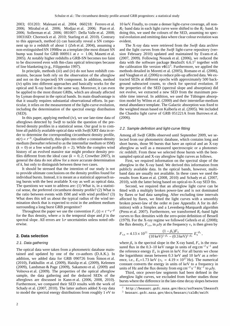
Table B.2. Light-curve parameters of the late-time optical and X-ray afterglows of the 27 bursts that entered our sample.

GRB Band Light-curve parameters Overlapping time intervaltlatestart (ks) tlate

end (ks) α1 α2 tb,jet (ks) tstart (ks) tend (ks)

O 33.33 196.67 . . . 1.97± 0.06050603 X 39.21 577.04 . . . 1.67± 0.05 < 39.2 39.2 196.7

O 0.25 106.27 1.19± 0.01 . . .050801 X 0.22 448.10 1.29± 0.08 . . .

> 106.3 0.25 106.3

O 23.89 612.10 1.04± 0.01 . . . . . .050820A X 4.64 3676.50 1.19± 0.02 1.73± 0.16 640.2± 138.7 23.9 612.1

O 4.13 606.01 1.47± 0.04 . . .050922C X 2.02 95.92 1.37± 0.03 . . .

> 95.9 4.1 95.9

O 17.52 265.20 1.03± 0.06 . . .051109A X 3.46 1240.80 1.20± 0.01 . . .

> 265.2 17.5 265.2

O 4.68 445.12 0.96± 0.03 . . . . . .051221AX 15.17 2271.92 1.03± 0.01 1.99± 0.17 318.5± 38.6

15.2 445.1

O 0.12 871.05 1.192± 0.002 . . .060418X 4.40 537.08 1.52± 0.05 . . .

> 537.1 4.4 537.1

O 7.02 715.56 0.80± 0.03 . . .060512X 0.24 288.61 1.12± 0.05 . . .

> 288.6 7.0 288.6

O 51.59 1700.19 1.05± 0.04 2.45± 0.05 113.1± 2.7060614X 41.23 1500.57 1.07± 0.11 2.31± 0.11 120.0± 12.1

51.6 1500.6

O 47.07 286.77 1.42± 0.18 . . .060714X 3.07 1029.03 1.23± 0.03 . . .

> 286.8 47.1 286.8

O 3.52 163.13 1.16± 0.02 . . .060904BX 3.58 391.01 1.36± 0.03 . . .

> 163.1 3.6 163.1

O 0.14 82.42 1.03± 0.01 . . .060908X 0.71 483.21 1.49± 0.07 . . .

> 82.4 0.71 82.4

O 92.09 523.12 1.29± 0.06 . . .070411X 0.50 664.68 1.12± 0.02 . . .

> 523.1 92.1 523.1

O 10.90 88.88 0.90± 0.16 . . .070802X 6.68 316.52 1.17± 0.09 . . .

> 88.9 10.9 88.9

O 1.95 103.36 1.30± 0.10 . . .070810AX 1.55 34.46 1.29± 0.07 . . .

> 34.5 1.9 34.5

O 0.8 1060 1.237± 0.002 . . .080319BX 42.66 2559.17 1.04± 0.05 2.68± 0.36 953± 137

42.7 1060

Notes. Columns 3 to 7 give the time interval,tlatestart, t

latestop, the pre- and post-jet break decay slopes,α1, α2, and the observed jet break time,tb,jet. The

optical and X-ray light curves were independently fitted forevery GRB (Sect. 2.2). Owing this, two break times are given for GRB 060614. Withinthe errors the break was achromatic, making it a good candidate for a jet break. For the other GRBs we state the upper or lower limits on the jetbreak time with respect to the identification of the dynamical regime shown in Table B.3. The overlapping time interval ofthe late-time opticaland X-ray afterglow is shown in the last two columns.† The optical afterglow light curve of GRB 080721 shows an additional shallow break at(129± 84) ks. The difference in the pre- and post-break decay slope is≈ 0.25 in agreement with Kann et al. (2010), which is typical for acoolingbreak. This break is not a jet break.

9


GRB BandLight-curve parameters Overlapping time interval

tstart (ks) tend (ks) α1 α2 tb,jet (ks) tstart (ks) tend (ks)

O 37.15 174.79 1.64± 0.06 . . .080514BX 37.30 217.27 1.54± 0.14 . . .

> 174.8 37.3 174.8

O 9.97 353.11 1.57± 0.02 . . .080710X 11.34 349.31 1.56± 0.09 . . .

> 349.3 11.3 349.3

O 0.17 2641.08 1.22± 0.01 1.46± 0.08080721†X 29.46 1256.83 1.50± 0.03 . . .

> 1256.8 29.5 1256.8

O 97.49 377.94 1.40± 0.10 . . .080916C X 65.03 1306.33 1.29± 0.08 . . .

> 377.9 97.5 377.9

O 6.60 301.54 . . . 1.72± 0.01 . . .081203A X 8.91 345.00 1.13± 0.01 1.93± 0.06 8.9± 0.9 8.9 301.5

O 15.76 263.68 1.50± 0.03 . . .090102 X 0.95 688.48 1.43± 0.02 . . .

> 263.6 15.8 263.7

O 96.81 1142.30 . . . 1.88± 0.01090323 X 70.47 1084.77 . . . 1.56± 0.10 < 96.8 96.8 1084.8

O 57.28 1007.14 . . . 1.78± 0.04090328 X 0.15 924.60 . . . 1.68± 0.09 < 57.3 57.3 924.6

O 1.40 10.00 0.97± 0.10 . . .090726 X 3.61 66.43 1.34± 0.04 . . .

> 10.0 3.6 10.0

O 45.64 1171.46 0.97± 0.02 . . .090902B X 45.21 1456.69 1.33± 0.03 . . .

> 1171.5 45.6 1171.5

O 254.24 2070.84 1.74± 0.02 . . .090926A X 51.49 1803.53 1.53± 0.07 . . .

> 1803.5 254.2 1803.5

Table B.2 — continued

10


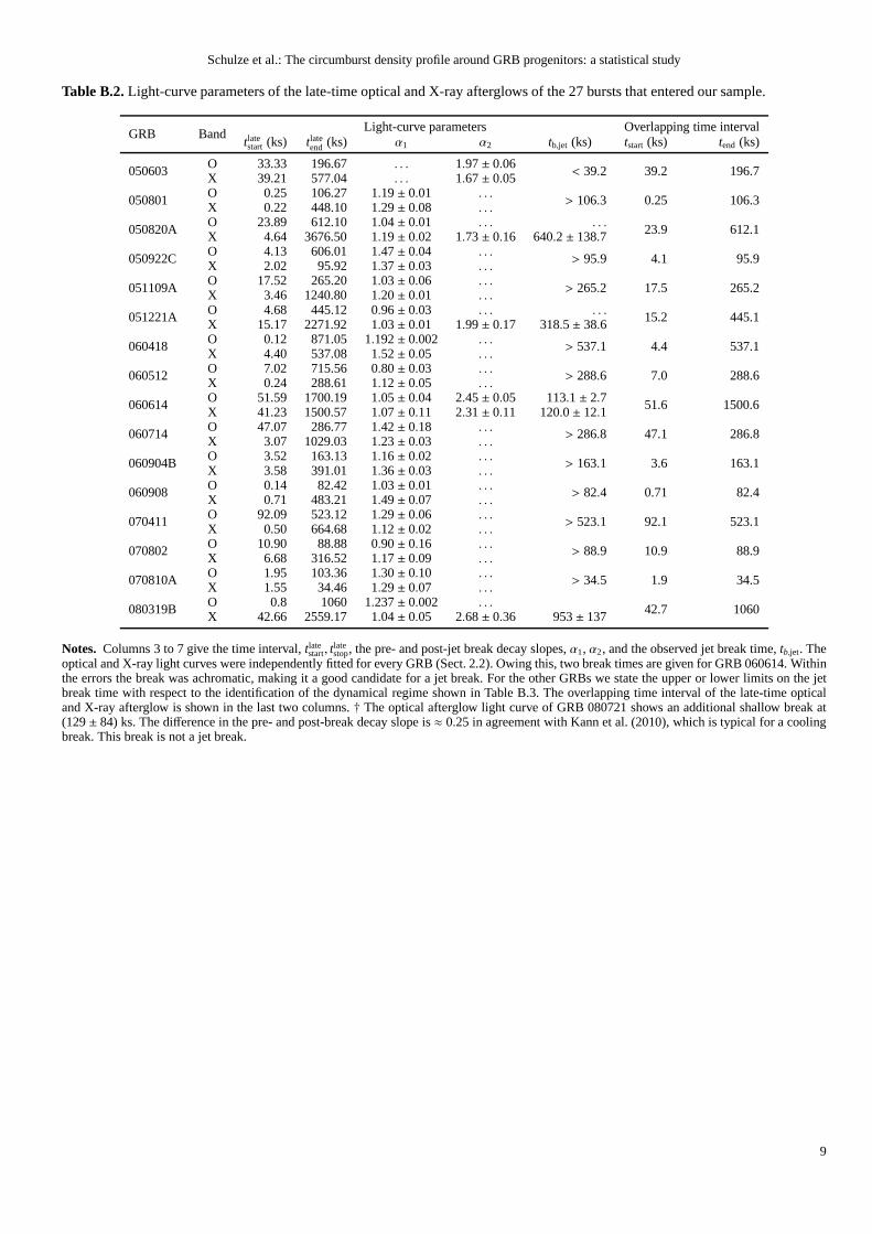
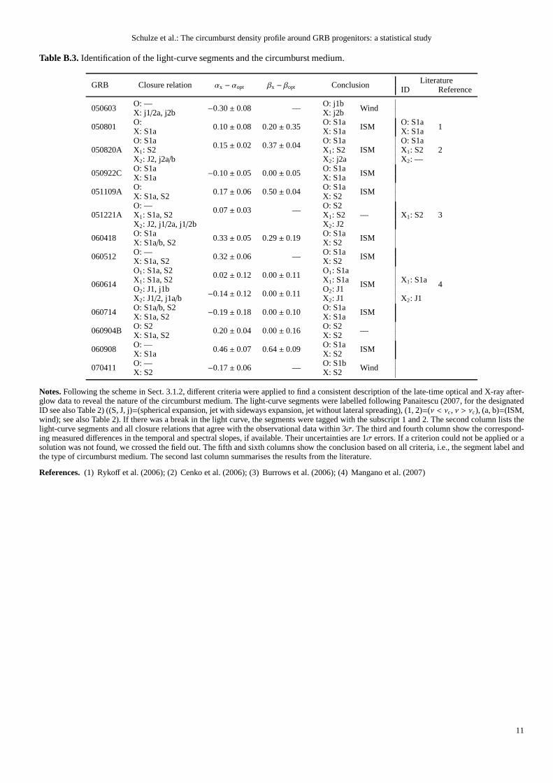
Table B.3. Identification of the light-curve segments and the circumburst medium.

GRB Closure relation αx − αopt βx − βopt Conclusion LiteratureID Reference

O: — O: j1b050603 X: j1/2a, j2b −0.30± 0.08 — X: j2b Wind

050801O: O: S1a O: S1aX: S1a 0.10± 0.08 0.20± 0.35 X: S1a ISM X: S1a 1

O: S1a O: S1a O: S1aX1: S2 0.15± 0.02 0.37± 0.04 X1: S2 X1: S2050820AX2: J2, j2a/b X2: j2a

ISMX2: —

2

050922CO: S1a O: S1aX: S1a −0.10± 0.05 0.00± 0.05 X: S1a ISM

O: O: S1a051109A

X: S1a, S20.17± 0.06 0.50± 0.04

X: S2ISM

O: — O: S2X1: S1a, S2

0.07± 0.03 —X1: S2 X1: S2051221A

X2: J2, j1/2a, j1/2b X2: J2— 3

O: S1a O: S1a060418X: S1a/b, S2

0.33± 0.05 0.29± 0.19X: S2

ISM

060512 O: — O: S1aX: S1a, S2

0.32± 0.06 —X: S2

ISM

O1: S1a, S2 O1: S1aX1: S1a, S2

0.02± 0.12 0.00± 0.11X1: S1a X1: S1a

O2: J1, j1b O2: J1060614

X2: J1/2, j1a/b−0.14± 0.12 0.00± 0.11

X2: J1

ISM

X2: J1

4

O: S1a/b, S2 O: S1a060714X: S1a, S2

−0.19± 0.18 0.00± 0.10X: S1a

ISM

O: S2 O: S2060904BX: S1a, S2

0.20± 0.04 0.00± 0.16X: S2

—

O: — O: S1a060908X: S1a

0.46± 0.07 0.64± 0.09X: S2

ISM

O: — O: S1b070411X: S2

−0.17± 0.06 —X: S2

Wind

Notes. Following the scheme in Sect. 3.1.2, different criteria were applied to find a consistent descriptionof the late-time optical and X-ray after-glow data to reveal the nature of the circumburst medium. Thelight-curve segments were labelled following Panaitescu (2007, for the designatedID see also Table 2) ((S, J, j)=(spherical expansion, jet with sideways expansion, jet without lateral spreading), (1, 2)=(ν < νc, ν > νc), (a, b)=(ISM,wind); see also Table 2). If there was a break in the light curve, the segments were tagged with the subscript 1 and 2. The second column lists thelight-curve segments and all closure relations that agree with the observational data within 3σ. The third and fourth column show the correspond-ing measured differences in the temporal and spectral slopes, if available. Their uncertainties are 1σ errors. If a criterion could not be applied or asolution was not found, we crossed the field out. The fifth and sixth columns show the conclusion based on all criteria, i.e., the segment label andthe type of circumburst medium. The second last column summarises the results from the literature.

References. (1) Rykoff et al. (2006); (2) Cenko et al. (2006); (3) Burrows et al. (2006); (4) Mangano et al. (2007)

11


GRB Closure relation αx − αopt βx − βopt ConclusionLiterature

ID Reference

O: S1a/b, S2 O: S1a O: S2070802X: S2

0.27± 0.18 0.50± 0.05X: S2

ISMX: S2

5

O: — O: S1a070810AX: S1a, S2

−0.01± 0.12 —X: S2

ISM

O: S1b O: S1b O: S1bX1:S1a, S2

−0.20± 0.05 0.48± 0.12X1: S2 X1: S2080319B

X2: X2: —Wind

X2: J26

O: S1b O: S1b O: S1b080514B X: S1a/b, S2 −0.10± 0.14 0.50± 0.13 X: S2 Wind X: S2 7

O: S1a, j2b O: S1a O: S1a080710 X: S1a, j2a/b −0.01± 0.09 0.00± 0.01 X: S1a ISM X: S1a 8

O1: — O1: S1a 1) O1: S1a; 2) O: S1aO2: — O2: S2 1) O2: S2080721X: S2 0.04± 0.09 — X: S2

ISM1) X: —; 2) X: S1a

1) 9; 2) 10

O: O: S1b O: S1a/b080916C X: −0.11± 0.13 0.00± 0.34 X: S1b Wind X: S1a/b 11

X1: S2 X1: S2O: — — O: j1a081203AX2: J2, j2a/b 0.21± 0.06 X2: j2a

ISM

O: O: S1a O: S1a090102 X: 0.07± 0.04 0.02± 0.22 X: S1a ISM X: S1a 12

O: S1b, j1a/b O: j1b 1) O: J1, j1a/b; 2) O: S1b090323 X: S1a/b, S2, j1/2a, j2b −0.32± 0.10 0.30± 0.18 X: j2b Wind 1) X: —; 2) X: S1b 1) 13; 2) 14

O: S1a/b, S2, j1a, j2a/b O: j2a O: J1090328 X: S1a/b, S2, j1a, j2a/b −0.10± 0.09 −0.07± 0.21 X: j2a ISM X: J1 13

O: — O: S1a O: S1a090726 X: S2 0.37± 0.10 — X: S2 ISM X: S2 15

O: S1a, S2 O: S1a O: S1a090902B X: S1a, S2 0.36± 0.04 0.29± 0.17 X: S2 ISM X: S2 13, 14

O: S1a/b O: S1a 1) O: S2; 2) O: S1a090926AX: S1a

−0.21± 0.07 0.00± 0.08X: S1a

ISM1) X: S2; 2) X: S1a

1) 14: 2) 16

References. (5) Kruhler et al. (2008); (6) Racusin et al. (2008); (7) Rossi et al. (2009); (8) Kruhler et al. (2009); (9) Kann et al. (2010);(10) Starling et al. (2009); (11) Greiner et al. (2009b); (12) Gendre et al. (2010); (13) McBreen et al. (2010); (14) Cenkoet al. (2010); (15)Simon et al. (2010); (16) Rau et al. (2010)

Table B.3 — continued

12


Appendix C: Figures of the light curve fits

13


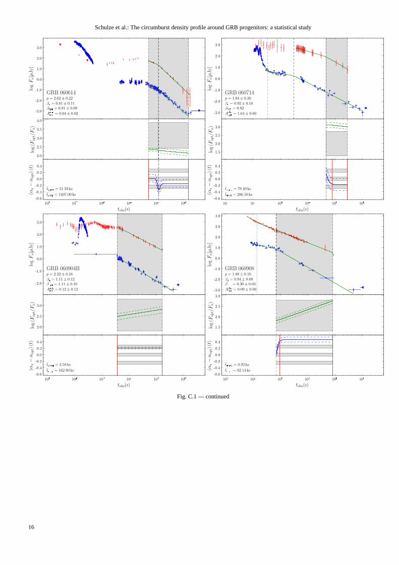
Fig. C.1. Optical and X-ray afterglow light curves of the 27 bursts that entered our sample.Upper panel: The optical data in theRcband are shown as dots and the X-ray data at 1.73 keV as bigger dots with an error bar in time. The light-curve fits are over-plotted.Upper limits are shown as downwards-pointing triangles. The grey box is the overlapping time interval of the late-time evolution.Vertical dotted and dashed lines indicate breaks in the optical and X-ray band. Information on the SEDs are shown in the bottom left(see also Table B.1). The given extinction,Ahost

opt , is the observed host-extinction in theRc band based on the deduced host extinctionin the V-band,Ahost

V . Additionally, we deduced the electron index,p, from βx. The electron index is eitherp = 2β if νc < νx orp = 2β + 1 if νc > νx (e.g., Zhang & Meszaros 2004). Its error was computed by propagating the uncertainty inβx. Middle panel:The flux density ratio between the optical and X-ray afterglow is shown as a solid line and its error as a dashed line for the sharedtime interval of the late-time evolution. The grey box represents the allowed parameter space of the flux density ratio (Table 1). Theupper boundary is the expected flux density ratio forνc ≤ νopt, while the lower one shows the expected ratio forνc ≥ νx. If thecooling break is in between the optical and the X-ray bands, the expected flux-density ratio lies be in between these boundaries.The expected flux density ratio depends on the electron index. Not all bursts could be corrected for host extinction. The error onthe electron index was neither propagated into the error of the expected nor of the observed flux-density ratio.Lower panel: Thefirst logarithmic derivative of the flux-density ratio,

(

αx − αopt

)

(t), is shown as a solid curve and its error is plotted as a dashedline. Fort/tbreak � 1, the first logarithmic derivative is identical to the difference in the decay slopes obtained from the light-curvefit (asymptotic values). Usually breaks in the light curves tend to be smooth instead of sharp. Because of this, the first logarithmicderivative deviates from the asymptotic value close to a break depending on the smoothness of the break. Two solid lines are plottedto highlight the time interval when the asymptotic decay slopes were reached within 1σ. The precise values are shown on the leftand in Table 3. Within 3σ, the asymptotic difference in the decay slopes agrees either with+1/4, 0,−1/4 depending on the spectraland dynamical regime and the circumburst density profile. Furthermore, an envelope is drawn around expected values,+1/4, 0,−1/4, with a width of 0.1 to guide the eye.

14


Fig. C.1 — continued

15



16



17



18



19



20

the circumburst density proﬁle around grb progenitors: a

Documents