The Causes and Consequences of House Price Momentum

Adam M. Guren�

Harvard University

April 17, 2014

First Version: November 10, 2013

Abstract

House price changes are positively autocorrelated over two to three years, a phenomenon

known as momentum. This paper introduces, empirically grounds, and quantitatively analyzes

an ampli�cation mechanism that can generate substantial momentum from small frictions and

demonstrates that the resulting momentum helps explain the short-run dynamics of housing

markets. The ampli�cation is due to a concave demand curve in relative price, which im-

plies that increasing the quality-adjusted list price of a house priced above the market average

rapidly reduces its probability of sale, but cutting the price of a below-average priced home

only slightly improves its chance of selling. This creates a strategic complementarity that in-

centivizes sellers to set their list price close to others�. Consequently, frictions that cause slight

insensitivities to changes in fundamentals lead to prolonged adjustments because sellers gradu-

ally adjust their price to stay near the average. I provide new micro empirical evidence for the

concavity of demand� which is often used in macro models with strategic complementarities�

by instrumenting a house�s relative list price with a proxy for the seller�s equity. I �nd signi�cant

concavity, which I embed in an equilibrium housing search model in which buyers avoid visiting

houses that appear overpriced. I demonstrate and quantitatively evaluate the model�s ability to

amplify two frictions: staggered pricing and a fraction of backwards-looking rule-of-thumb sell-

ers. Both frictions are ampli�ed substantially, and the model explains the momentum observed

empirically with a small fraction of rule-of-thumb sellers. Strong house price momentum leads

households to re-time their purchase or sale, thereby explaining several features of the dynamic

relationships between price, volume, inventory, and buyer and seller entry.

�Email: guren@fas.harvard.edu. I would like to thank John Campbell, Raj Chetty, Emmanuel Farhi, EdwardGlaeser, Nathaniel Hendren, and Lawrence Katz for their advice and guidance. Gary Chamberlain, John Friedman,James Hamilton, Max Kasy, Jonathan Parker, Alp Simsek, Andrei Shleifer, and Lawrence Summers also providedthoughtful discussions and comments. Nikhil Agarwal, Rebecca Diamond, Will Diamond, Peter Ganong, Ben Hebert,Michal Kolesar, Tim McQuade, Pascal Noel, Mikkel Plagborg-Moller, Ben Schoefer, and seminar participants atHarvard provided numerous discussions and suggestions. Andrew Cramond at DataQuick, Mike Simonsen at AltosResearch, T.J. Doyle at the National Association of Realtors, and Mark Fleming, Sam Khater, and Kathryn Dobbynat CoreLogic assisted me in understanding their data. Shelby Lin and Christopher Palmer provided assistance withthe DataQuick data.

1 Introduction

A puzzling and prominent feature of housing markets is that aggregate price changes are highly

positively autocorrelated, with a one percent annual price change correlated with a 0.30 to 0.75

percent change in the subsequent year (Case and Shiller, 1989).1 This price momentum lasts for two

to three years before prices mean revert, a time horizon far greater than most other asset markets.

Substantial momentum is surprising because predictable price changes should be arbitraged away by

investors and households that can re-time their purchase or sale and because most pricing frictions

dissipate quickly.

This paper introduces, empirically grounds, and quantitatively analyzes an ampli�cation mech-

anism that can generate substantial momentum from small frictions. The mechanism relies on a

strategic complementarity among list-price-setting sellers that makes the optimal list price for a

house depend positively on the prices set by others (Cooper and John, 1988). Strategic comple-

mentarities of this sort are frequently used in macroeconomic models (e.g., Ball and Romer, 1990;

Woodford, 2003; Angeletos and La�O, 2013) but there is limited empirical evidence of their im-

portance and strength. In analyzing momentum in the housing market, I provide micro empirical

evidence for a prevalent strategic complementarity in the macroeconomics literature and, using a

calibrated equilibrium search model, demonstrate that its ability to amplify underlying frictions is

quantitatively signi�cant.

I also show that momentum has important consequences that help explain several perplex-

ing features of the dynamics of housing markets relating to sales and inventory in addition to

price. These dynamics, which are analogous to several features of business cycles, matter for the

macroeconomy because housing markets a¤ect household balance sheets, the �nancial system, and

business cycles and are a potential channel for monetary policy. House price momentum may also

explain why recoveries from housing-triggered cycles are slow.

The propagation mechanism I introduce relies on two components: costly search and a demand

curve that is concave in relative price. Search is inherent to housing because no two houses are

alike and idiosyncratic taste can only be learned through costly inspection. Search and idiosyncratic

taste also limit arbitrage by creating endogenous transaction costs and by making the market price

for a house di¢ cult to ascertain. Concave demand in relative price implies that the probability a

house sells is more sensitive to list price for houses priced above the market average than below

the market average. While concave demand may arise in housing markets for several reasons, I

focus on the manner in which asking prices direct buyer search. The intuition is summarized by

an advice column for sellers: �Put yourself in the shoes of buyers who are scanning the real estate

ads...trying to decide which houses to visit in person. If your house is overpriced, that will be an

immediate turno¤. The buyer will probably clue in pretty quickly to the fact that other houses

look like better bargains and move on.�2 In other words, the probability that a house is visited by

1See also Cutler et al. (1991), Abraham and Hendershott (1996), Cho (1996), Malpezzi (1999), Meen (2002),Capozza et al. (2004), Head et al. (2014), and Glaeser et al. (2013).

2�Settling On The Right List Price for Your House,�Ilona Bray, http://www.nolo.com/legal-encyclopedia/listing-

1

buyers decreases rapidly as a home�s list price rises relative to the market average. This generates

a concave demand curve in relative price because at high relative prices buyers are on the margin

of looking and purchasing, while at low relative prices they are only on the margin of purchasing.

Concave demand incentivizes list-price-setting sellers� who have market power due to search

frictions� to set their list prices close to the mean. Intuitively, raising a house�s relative list price

reduces the probability of sale and pro�t dramatically, while lowering its relative price increases

the probability of sale slightly and leaves money on the table. Modest frictions that generate initial

insensitivities of prices to changes in fundamentals cause protracted price adjustments because

sellers �nd it optimal to gradually adjust their price so that they do not stray too far from the

market average.

To evaluate the concavity of the e¤ect of unilaterally changing a house�s relative quality-adjusted

price on its sales probability, I turn to micro data on listings for the San Francisco Bay, Los Angeles,

and San Diego metropolitan areas from 2008 to 2013. I address bias caused by unobserved quality

by instrumenting relative list price with the amount of aggregate price appreciation since the seller

purchased. The identi�cation strategy takes advantage of the fact that sellers with low appreciation

since purchase set higher list prices because the equity they extract from the sale of their current

home constrains their ability to make a down payment on their next home (Stein, 1995; Genesove

and Mayer, 1997). Because I compare listings within a ZIP code and quarter, this supply-side

variation identi�es the curvature of demand if unobserved quality is independent of when a seller

purchased their home. The instrumental variable estimates reveal a concave relationship that is

statistically and economically signi�cant.3 My �ndings about the concavity of demand are robust

to other sources of relative price variation that are independent of appreciation since purchase.

To assess the strength of this propagation mechanism, I embed concave demand in a Diamond-

Mortensen-Pissarides equilibrium search model. I explore the e¤ects of two separate sources of price

insensitivity. First, I consider staggered pricing whereby overlapping groups of sellers set prices

that are �xed for multiple periods (Taylor, 1980). Concave demand induces sellers to only partially

adjust their prices when they have the opportunity to do so, and repeated partial adjustment

manifests itself as additional momentum. Second, I introduce a small fraction of backward-looking

rule-of-thumb sellers as in Campbell and Mankiw (1989) and Gali and Gertler (1999). Backward-

looking expectations are frequently discussed as a potential cause of momentum (e.g., Case and

Shiller, 1987; Case et al. 2012), but some observers have voiced skepticism about widespread

non-rationality in housing markets given the �nancial importance of housing transactions for most

households. With a strategic complementarity, far fewer backward-looking sellers are needed to

explain momentum because the majority of forward-looking sellers adjust their prices gradually so

they do not deviate too much from the backward-looking sellers (Haltiwanger and Waldman, 1989;

Fehr and Tyran, 2005). This, in turn, causes the backward-looking sellers to observe more gradual

price growth and change their price by less, creating a two-way feedback that ampli�es momentum.

house-what-price-should-set-32336-2.html.3Although endogeneity is a worry, the ordinary least squares relationship is also concave. However, as one would

expect if unobservable quality is an issue, it has a smaller slope.

2

I calibrate the parameters of the model that control the shape of the demand curve to match the

micro empirical estimates and the remainder of the model to match steady state and time series

moments. The calibrated model generates substantial ampli�cation of the underlying frictions.

With staggered pricing, the model can explain a ten month price adjustment� or about one quarter

of the momentum in the data� in response to a shock to fundamentals even though all sellers have

reset their price within two months of the shock. With rule-of-thumb sellers, the model generates

three years of positively autocorrelated price changes as observed empirically if 26.5 percent of

sellers are backward-looking. By contrast, without concave demand, 78 to 93 percent of sellers

would have to be backward-looking to generate a three-year response.

The ampli�cation mechanism adapts two ideas from the macro literature on goods price sticki-

ness to frictional asset search. First, the concave demand curve is similar to �kinked�demand curves

(Stiglitz, 1979; Woglom, 1982) which, since the pioneering work of Ball and Romer (1990) has been

frequently cited as a potential source of real rigidities. In particular, a �smoothed-out kink� ex-

tension of Dixit-Stiglitz preferences proposed by Kimball (1995) is frequently used to tractably

introduce real rigidities through strategic complementarity in price setting. Second, the repeated

partial price adjustment caused by the strategic complementarity is akin to Taylor�s (1980) �con-

tract multiplier.�A lively literature has debated the importance of strategic complementarities and

kinked demand in particular for propagating goods price stickiness by analyzing calibrated models

(e.g., Chari et al., 2000), by assessing whether the rami�cations of strategic complementarities are

borne out in micro data (Klenow and Willis, 2006; Bils et al., 2012), and by examining exchange-

rate pass through for imported goods (e.g., Gopinath and Itshoki, 2010; Nakamura and Zerom,

2010). My analysis of housing markets adds to this literature by directly estimating a concave

demand curve and assessing its ability to amplify frictions in a calibrated model.

Having established a propagation mechanism for house price momentum empirically and theo-

retically, I show that momentum a¤ects the dynamics of sales volume and the inventory of houses

for sale. Forward-looking buyers and sellers re-time their purchase decisions due to expectations

of predictable future price changes. Such re-timing causes sudden swings in inventory that drive

the reversal between a hot market, with a substantial excess of buyers, and a cold market, with

a relative dearth of buyers. For instance, at a trough, marginal buyers rush to purchase before

prices rise, while marginal sellers wait to obtain a better price for their home, leading inventory

to plummet.4 To formalize this story, I build on Novy-Marx (2009) by including buyer and seller

entry decisions in the model.

Forward-looking entry responses in the calibrated model help explain three puzzling features of

housing cycles. First, seller entry remains high as volume plummets at peaks and remains low as

4Buyer and seller quotes in newspapers provide suggestive evidence of such re-timing. In 2013, when prices wererising, a buyer explained to the Wall Street Journal �if you don�t get in now, things are going to skyrocket over thenext year,�while a seller who delayed putting their house on the market told the Journal that �the extra money �that was worth [waiting] for the year.�This e¤ect is part of the folk wisdom of housing markets, yet has not appearedin the academic literature. For instance, Calculated Risk Blog describes a conversation with a real estate agent whoargues that �In a market with falling prices, sellers rush to list their homes, and inventory increases. But if sellersthink prices have bottomed, then they believe they can be patient, and inventory declines.�

3

volume picks up at troughs, which is the exact pattern created by the re-timing of entry in light

of momentum. Second, volume and inventory are more volatile than price. This is di¢ cult to

reconcile with most calibrations of housing search models in a direct analogue to Shimer�s (2005)

unemployment volatility puzzle for labor search models. With momentum, volume and inventory

are more volatile not only because price responds gradually but also because the adjustment of

inventory is accelerated by the re-timing of entry. Third, in the data, price changes are strongly

negatively correlated with inventory levels (Peach, 1983). This �housing Phillips curve�is surprising

because in most asset pricing models, price changes are correlated with changes in fundamentals

such as inventory (Caplin and Leahy, 2011). In my model, the quick response of inventory and

gradual response of price create a strong correlation between price changes and inventory levels.

The remainder of the paper proceeds as follows. Section 2 introduces facts about housing

dynamics. Section 3 analyzes micro data to assess whether housing demand curves are concave.

Section 4 presents the model. Section 5 calibrates the model to the micro estimates and assesses

the degree to which strategic complementarities amplify momentum. Section 6 discusses the con-

sequences of this momentum for housing cycles. Section 7 concludes.

2 Four Facts About Housing Dynamics

2.1 Momentum

Since the pioneering work of Case and Shiller (1989), price momentum has been considered one of

the most puzzling features of housing markets. While other �nancial markets exhibit momentum,

the housing market is unusual for the strength of the e¤ect and the horizon over which it persists.5

Fact 1: Price changes are serially correlated for 8 to 14 quarterly lags.House price momentum has consistently been found across cities and countries, time periods, and

price index measurement methodologies (Cho, 1996). Figure 1 shows three measures of momentum

for the CoreLogic national repeat-sales house price index for 1976 to 2013.6 Panel A shows that

autocorrelations are positive for 11 quarterly lags of the quarterly change in the price index adjusted

for in�ation and seasonality. Panel B shows an impulse response in log levels to an initial one

percent price shock estimated from an AR(5). In response to the shock, prices gradually rise for

two to three years before mean reverting. Finally, panel C shows a histogram of AR(1) coe¢ cients

estimated separately for 103 metropolitan area repeat-sales house price indices from CoreLogic

using a regression of the annual change in log price on a one-year lag of itself as in Case and Shiller

5Note that the �momentum� I analyze refers to autocorrelation in aggregate price time series, which is distinctfrom the short-term over-performance of stocks that recently performed best that is also called �momentum.�Time-series momentum holds for a number of other asset classes over shorter horizons. Cutler et al. (1991) look across alarge number of asset classes and �nd that for the vast majority of assets, positive autocorrelation in returns lastsfor less than a year. Moskowitz et al. (2012) �nd that time series momentum lasts for approximately 12 months for58 di¤erent equity index, currency, commodity, and bond futures. This 12 month horizon is an upper bound for thetype of momentum studied here, which includes only capital gains, because the measured returns in Moskowitz et al.include both dividends (which are known to be autocorrelated) and capital gains.

6As discussed in Appendix B, price indices that measure the median price of transacted homes display momentumover roughly two years as opposed to three years for repeat-sales indices.

4

Figure 1: Momentum in Housing Prices

Notes: Panel A and B show the autocorrelation function for quarterly real price changes and an impulse response of log real

price levels estimated from an AR(5) model, respectively. The IRF has 95% con�dence intervals shown in grey. An AR(5) was

chosen using a number of lag selection criteria, and the results are robust to altering the number of lags. Both are estimated

using the CoreLogic national repeat-sales house price index from 1976-2013 collapsed to a quarterly level, adjusted for in�ation

using the CPI, and seasonally adjusted. Panel C shows a histogram of annual AR(1) coe¢ cients of annual house price changes

as in regression (1) estimated separately on 103 CBSA division repeat-sales house price indices provided by CoreLogic. The

local HPIs are adjusted for in�ation using the CPI. The 103 CBSAs and their time coverage, which ranges from 1976-2013 to

1995-2013, are listed in Appendix A.

(1989):

�t;t�4 ln p = �0 + �1�t�4;t�8 ln p+ ". (1)

�1 is positive for all 103 cities, strongest for cities with inelastic housing supply, and the median

city has an annual AR1 coe¢ cient of 0.60. Appendix B replicates these facts for a number of

countries, price series, and measures of autocorrelation and consistently �nds two to three years of

momentum.7

The existing evidence suggests that momentum cannot be explained by serially correlated

7 In the housing market, the price level appears to be sticky but the rate of change does not appear to reactsluggishly. In particular, neither the evidence presented here nor the structural panel VAR in Head et al. (2014)shows evidence of autocorrelations of house price changes near one or delayed �hump shaped� impulse responses ofhouse price changes. This is unlike the CPI or GDP de�ator, which demonstrate considerable persistence in the rateof change (Fuhrer, 2011).

5

changes in fundamentals. Case and Shiller (1989) argue that momentum cannot be explained

by autocorrelation in interest rates, rents, or taxes. Glaeser et al. (2013) estimate a dynamic

spatial equilibrium model and �nd that �there is no reasonable parameter set� consistent with

short-run momentum. Capozza et al. (2004) �nd signi�cant momentum after accounting for six

comprehensive measures of fundamentals in a vector error correction model.

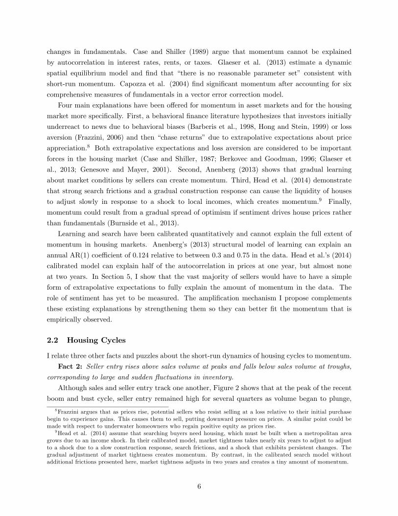
Four main explanations have been o¤ered for momentum in asset markets and for the housing

market more speci�cally. First, a behavioral �nance literature hypothesizes that investors initially

underreact to news due to behavioral biases (Barberis et al., 1998, Hong and Stein, 1999) or loss

aversion (Frazzini, 2006) and then �chase returns�due to extrapolative expectations about price

appreciation.8 Both extrapolative expectations and loss aversion are considered to be important

forces in the housing market (Case and Shiller, 1987; Berkovec and Goodman, 1996; Glaeser et

al., 2013; Genesove and Mayer, 2001). Second, Anenberg (2013) shows that gradual learning

about market conditions by sellers can create momentum. Third, Head et al. (2014) demonstrate

that strong search frictions and a gradual construction response can cause the liquidity of houses

to adjust slowly in response to a shock to local incomes, which creates momentum.9 Finally,

momentum could result from a gradual spread of optimism if sentiment drives house prices rather

than fundamentals (Burnside et al., 2013).

Learning and search have been calibrated quantitatively and cannot explain the full extent of

momentum in housing markets. Anenberg�s (2013) structural model of learning can explain an

annual AR(1) coe¢ cient of 0.124 relative to between 0.3 and 0.75 in the data. Head et al.�s (2014)

calibrated model can explain half of the autocorrelation in prices at one year, but almost none

at two years. In Section 5, I show that the vast majority of sellers would have to have a simple

form of extrapolative expectations to fully explain the amount of momentum in the data. The

role of sentiment has yet to be measured. The ampli�cation mechanism I propose complements

these existing explanations by strengthening them so they can better �t the momentum that is

empirically observed.

2.2 Housing Cycles

I relate three other facts and puzzles about the short-run dynamics of housing cycles to momentum.

Fact 2: Seller entry rises above sales volume at peaks and falls below sales volume at troughs,corresponding to large and sudden �uctuations in inventory.

Although sales and seller entry track one another, Figure 2 shows that at the peak of the recent

boom and bust cycle, seller entry remained high for several quarters as volume began to plunge,

8Frazzini argues that as prices rise, potential sellers who resist selling at a loss relative to their initial purchasebegin to experience gains. This causes them to sell, putting downward pressure on prices. A similar point could bemade with respect to underwater homeowners who regain positive equity as prices rise.

9Head et al. (2014) assume that searching buyers need housing, which must be built when a metropolitan areagrows due to an income shock. In their calibrated model, market tightness takes nearly six years to adjust to adjustto a shock due to a slow construction response, search frictions, and a shock that exhibits persistent changes. Thegradual adjustment of market tightness creates momentum. By contrast, in the calibrated search model withoutadditional frictions presented here, market tightness adjusts in two years and creates a tiny amount of momentum.

6

Figure 2: Sales, Entry and Inventory, 2003-2013

1.2

1.4

1.6

1.8

22.

2H

omes

 Lis

ted 

For S

ale 

(Mill

ions

)

800

1000

1200

1400

1600

Qua

rterly

 Sal

es o

r Ent

ry (M

illio

ns)

2003 2008 2013Year

Volume Seller EntryImputed Buyer Entry Homes Listed For Sale

Notes: Volume is raw data from the National Association of Realtors of sales of existing single-family homes at a seasonally-

adjusted annual rate. Homes listed for sale is from the Census Vacancy Survey. Seller entry is computed as Entrantst = Sellerst

- Sellerst�1 + Salest. Buyer entry is computed similarly, but since there is not a raw data series for the stock of buyers it is

imputed using a simple Cobb-Douglas matching function SalesS = �

�BS

��:8with the 0.8 elasticity from Genesove and Han

(2012). In this �gure, � = 1 so that in a steady state there is 3 months of supply. All four series are smoothed using athree-quarter moving average.

which corresponded to a sudden increase in inventory. Conversely, as volume and prices began

to rise in 2012 and 2013, seller entry remained low, coinciding with a sudden drop in inventory.

Appendix B shows that this fact is not unique to 2003 to 2013. Although there is no data on

the stock of buyers, most models imply that if seller entry lags sales, buyer entry must lead sales.

Figure 2 illustrates this by using a simple matching function parameterized based on Genesove and

Han (2012) to infer the stock of buyers from sales volume and the stock of homes for sale.

Fact 3: At an annual frequency, the volatility of sales volume is twice that of real price and thevolatility of inventory as measured by months of supply is three times that of real price.

Despite the predictability of price changes, the housing market is volatile. Table 1 shows the

standard deviation of annual log changes for four series: real disposable personal income, real house

prices, sales volume, and �for sale� inventory measured as months of supply (a common metric

in the housing market). Price is four times more volatile than income, and volume and inventory

are, in turn, more volatile than price. The volatility of inventory in particular is of note because

substantial �uctuations in inventory at peaks and troughs herald rapid changes between buyers�and

sellers�markets. Finally, price and volume are highly positively correlated and both are positively

7

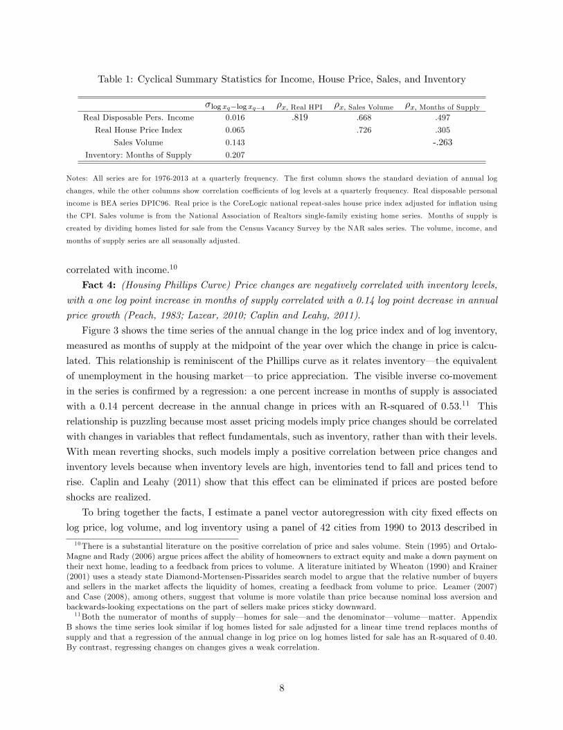
Table 1: Cyclical Summary Statistics for Income, House Price, Sales, and Inventory

�log xq�log xq�4 �x, Real HPI �x, Sales Volume �x; Months of SupplyReal Disposable Pers. Income 0.016 .819 .668 .497

Real House Price Index 0.065 .726 .305

Sales Volume 0.143 -.263Inventory: Months of Supply 0.207

Notes: All series are for 1976-2013 at a quarterly frequency. The �rst column shows the standard deviation of annual log

changes, while the other columns show correlation coe¢ cients of log levels at a quarterly frequency. Real disposable personal

income is BEA series DPIC96. Real price is the CoreLogic national repeat-sales house price index adjusted for in�ation using

the CPI. Sales volume is from the National Association of Realtors single-family existing home series. Months of supply is

created by dividing homes listed for sale from the Census Vacancy Survey by the NAR sales series. The volume, income, and

months of supply series are all seasonally adjusted.

correlated with income.10

Fact 4: (Housing Phillips Curve) Price changes are negatively correlated with inventory levels,with a one log point increase in months of supply correlated with a 0.14 log point decrease in annual

price growth (Peach, 1983; Lazear, 2010; Caplin and Leahy, 2011).

Figure 3 shows the time series of the annual change in the log price index and of log inventory,

measured as months of supply at the midpoint of the year over which the change in price is calcu-

lated. This relationship is reminiscent of the Phillips curve as it relates inventory� the equivalent

of unemployment in the housing market� to price appreciation. The visible inverse co-movement

in the series is con�rmed by a regression: a one percent increase in months of supply is associated

with a 0.14 percent decrease in the annual change in prices with an R-squared of 0.53.11 This

relationship is puzzling because most asset pricing models imply price changes should be correlated

with changes in variables that re�ect fundamentals, such as inventory, rather than with their levels.

With mean reverting shocks, such models imply a positive correlation between price changes and

inventory levels because when inventory levels are high, inventories tend to fall and prices tend to

rise. Caplin and Leahy (2011) show that this e¤ect can be eliminated if prices are posted before

shocks are realized.

To bring together the facts, I estimate a panel vector autoregression with city �xed e¤ects on

log price, log volume, and log inventory using a panel of 42 cities from 1990 to 2013 described in

10There is a substantial literature on the positive correlation of price and sales volume. Stein (1995) and Ortalo-Magne and Rady (2006) argue prices a¤ect the ability of homeowners to extract equity and make a down payment ontheir next home, leading to a feedback from prices to volume. A literature initiated by Wheaton (1990) and Krainer(2001) uses a steady state Diamond-Mortensen-Pissarides search model to argue that the relative number of buyersand sellers in the market a¤ects the liquidity of homes, creating a feedback from volume to price. Leamer (2007)and Case (2008), among others, suggest that volume is more volatile than price because nominal loss aversion andbackwards-looking expectations on the part of sellers make prices sticky downward.11Both the numerator of months of supply� homes for sale� and the denominator� volume� matter. Appendix

B shows the time series look similar if log homes listed for sale adjusted for a linear time trend replaces months ofsupply and that a regression of the annual change in log price on log homes listed for sale has an R-squared of 0.40.By contrast, regressing changes on changes gives a weak correlation.

8

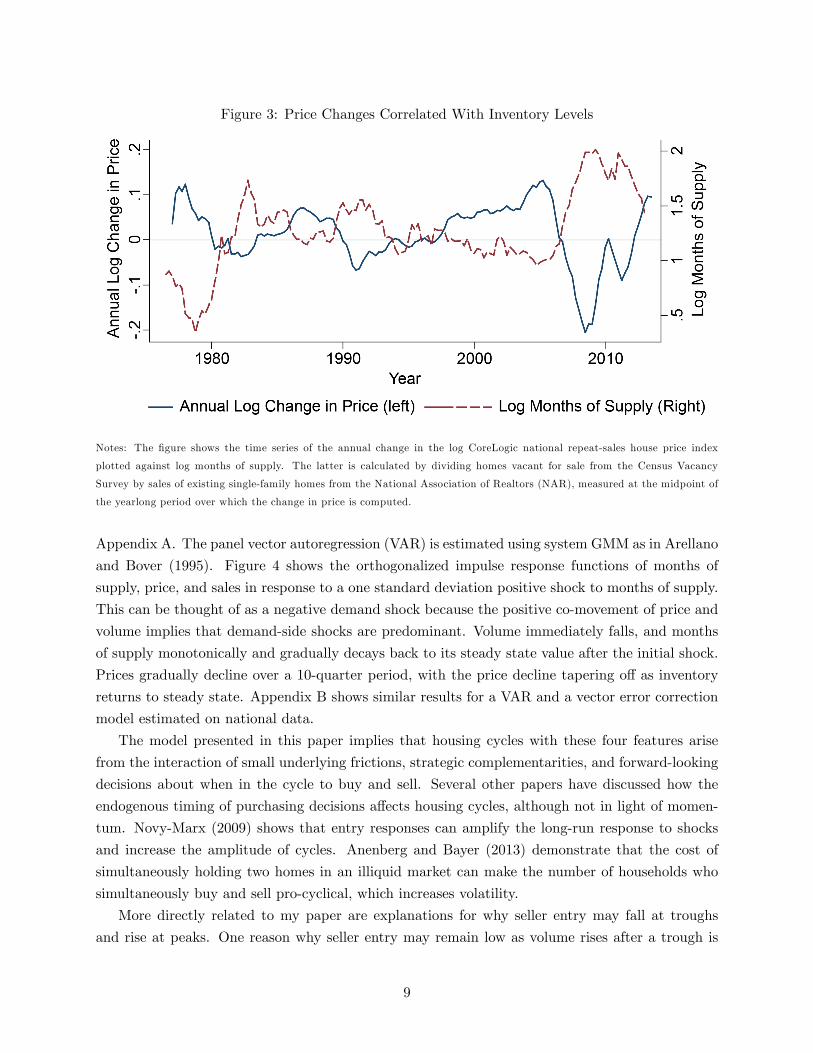
Figure 3: Price Changes Correlated With Inventory Levels

Notes: The �gure shows the time series of the annual change in the log CoreLogic national repeat-sales house price index

plotted against log months of supply. The latter is calculated by dividing homes vacant for sale from the Census Vacancy

Survey by sales of existing single-family homes from the National Association of Realtors (NAR), measured at the midpoint of

the yearlong period over which the change in price is computed.

Appendix A. The panel vector autoregression (VAR) is estimated using system GMM as in Arellano

and Bover (1995). Figure 4 shows the orthogonalized impulse response functions of months of

supply, price, and sales in response to a one standard deviation positive shock to months of supply.

This can be thought of as a negative demand shock because the positive co-movement of price and

volume implies that demand-side shocks are predominant. Volume immediately falls, and months

of supply monotonically and gradually decays back to its steady state value after the initial shock.

Prices gradually decline over a 10-quarter period, with the price decline tapering o¤ as inventory

returns to steady state. Appendix B shows similar results for a VAR and a vector error correction

model estimated on national data.

The model presented in this paper implies that housing cycles with these four features arise

from the interaction of small underlying frictions, strategic complementarities, and forward-looking

decisions about when in the cycle to buy and sell. Several other papers have discussed how the

endogenous timing of purchasing decisions a¤ects housing cycles, although not in light of momen-

tum. Novy-Marx (2009) shows that entry responses can amplify the long-run response to shocks

and increase the amplitude of cycles. Anenberg and Bayer (2013) demonstrate that the cost of

simultaneously holding two homes in an illiquid market can make the number of households who

simultaneously buy and sell pro-cyclical, which increases volatility.

More directly related to my paper are explanations for why seller entry may fall at troughs

and rise at peaks. One reason why seller entry may remain low as volume rises after a trough is

9

Figure 4: Impulse Response to Inventory Shock in Panel VAR0.

00.

10.

2Lo

g D

evia

tion 

Res

ultin

g Fr

om S

hock

0 4 8 12Quarters

Months of Supply

­0.0

5­0

.03

0.00

0 4 8 12Quarters

Price

­0.0

50.

00

0 4 8 12Quarters

Sales

Notes: The �gure shows orthogonalized impulse response functions to a months of supply shock computed from a two-lag

panel vector autoregression of log months of supply, log price, and log sales volume for a panel of 42 cities from 1990 to 2013

described in Appendix A. Price and sales are from CoreLogic, with price corresponding to the local CoreLogic house price

index adjusted for the CPI and sales corresponding to existing home sales. Months of supply at the MSA level comes from the

National Association of Realtors. All data is seasonally adjusted, and the panel VAR, which includes a �xed e¤ect for each

city as described in Appendix B, is estimated using system GMM and Helmert mean di¤erencing using a Stata package by

Inessa Love. The OIRFs are computed using a Cholesky decomposition with the variables ordered so that months of supply is

assumed not to depend contemporaneously on shocks to price or volume and price is assumed not to depend contemporaneously

on shocks to volume. The results are robust as long as months of supply is prior to volume in the Cholesky ordering. The blue

line is the OIRF, and the grey bands indicate 95 percent con�dence intervals computed using a Monte Carlo procedure that

generates 500 impulse responses from draws from the distribution of coe¢ cients implied by the estimated coe¢ cients and their

variance-covariance matrix.

nominal loss aversion (Genesove and Mayer, 2001) and lock in due to negative equity (Stein, 1995).

Head et al. (2014) present another mechanism: when local incomes rise, new entrants to an MSA

need a place to live, which drives up rents until new homes are built and causes potential sellers to

rent their homes temporarily before selling then. More broadly, Head et al. (2014) is most closely

related to this research. Their analysis of the joint responses of construction, house prices, house

sales, and population to city-level income shocks in a model with momentum is complementary to

my focus on the timing of purchase and sale decisions of existing homeowners and residents.

3 Are Housing Demand Curves Concave?

I propose an ampli�cation channel for momentum based on search and a concave demand curve in

relative price. Search is a natural assumption for housing markets, but the relevance of concave

demand requires further explanation.

A literature in macroeconomics shows how strategic complementarities among goods producers

10

can amplify small pricing frictions into substantial price sluggishness by incentivizing �rms to set

prices close to one another. Strategic complementarities operate either through a monopolistic

�rm�s marginal cost or its markup, which pushes a �rm to price close to the market average if

demand is concave in relative price. �Kinked demand� was introduced by Stiglitz (1979) and

Woglom (1982), who hypothesized that �rms that increase their price induce consumers to search

for a new �rm, but �rms that cut their price only gain a few active searchers. Ball and Romer

(1990) show that this can create real rigidities and possibly explain why prices are so sticky despite

small menu costs. This argument has been formalized in several papers, such as Benabou (1992)

and Levin and Yun (2009). Kimball (1995) generalizes Dixit-Stiglitz-style aggregator to allow for

concave demand, which is used as an important real rigidity in several popular New Keynesian

models (e.g., Smets and Wouters, 2007). Despite the frequency with which it is used, there is little

direct evidence for concave demand.12

Because momentum is similar to price stickiness in goods markets, I hypothesize that a similar

strategic complementarity may amplify house price momentum. There are several reasons why

concave demand may arise in housing markets. First, buyers may avoid visiting homes that appear

to be overpriced. Second, buyers may infer that underpriced homes are lemons. Third, a house�s

relative list price may be a signal of seller type, such as an unwillingness to negotiate (Albrecht et al.,

2013). Fourth, homes with high list prices may be less likely to sell quickly and may consequently

be more exposed to the tail risk of becoming a �stale�listing that sits on the market without selling

(Taylor, 1999). Fifth, buyers may infer that underpriced homes have a higher e¤ective price than

their list price because their price is likely to be increased in a bidding war (Han and Strange,

2012b).

Nonetheless, concrete evidence is needed for the existence of concave demand in housing markets

before it is adopted as an explanation for momentum. Consequently, this section assesses whether

demand is concave by analyzing micro data on listings matched to sales outcomes for the San

Francisco Bay, Los Angeles, and San Diego metropolitan areas from April 2008 to February 2013.13

The relevant demand curve for list-price-setting sellers is the e¤ect of unilaterally changing a

house�s relative quality-adjusted list price relative on its probability of sale. Detecting a nonlinear

e¤ect is challenging because quality is poorly measured, list prices are endogenous, and market

conditions vary. The principal econometric challenge is that quality di¤erences unobserved to the

econometrician lead to an estimated demand curve that is far more inelastic than the true demand

curve. The analysis is also complicated by the high number of foreclosures and short sales during

the period that I analyze. Short sales, which occur when a home is sold for less than the outstanding

mortgage balance, are especially worrisome because they often involve lengthy negotiations between

12Gopinath and Itshoki (2010) review both the price microdata and exchange rate pass-through literatures andargue there is a collage of evidence supporting a role for strategic complementarity in wholesale prices, but not resaleprices. The most direct evidence to date comes from Nakamura and Zerom (2010), who directly estimate the �superelasticity� (rate of change of the elasticity) of demand for co¤ee using a random coe¢ cients structural model and�nd evidence for concave demand.13These metro areas were selected because both the listings and transactions data providers are based in California,

so the matched dataset for these areas is of high quality and spans a longer time period.

11

the seller and their mortgage servicer which arti�cially decrease the probability of sale.

To surmount these challenges, I use a non-linear instrumental variable approach that traces out

the demand curve using plausibly exogenous supply-side variation in seller pricing behavior. Before

explaining the econometric strategy and presenting my main estimates, I �rst discuss the data.

3.1 Data

I combine data on listings with data on housing characteristics and transactions. The details of

data construction can be found in Appendix A. The listings data come from Altos Research, which

every Friday records a snapshot of homes listed for sale on multiple listing services (MLS) from

several publicly available web sites and records the address, MLS identi�er, and list price. The

housing characteristics and transactions data come from DataQuick, which collects and digitizes

public records from county register of deeds and assessor o¢ ces. This data provides a rich one-time

snapshot of housing characteristics from 2013 along with a detailed transaction history of each

property from 1988 to 2013 that includes transaction prices, loans, buyer and seller names and

characteristics, and seller distress. I limit my analysis to non-partial transactions of single-family

existing homes as categorized by DataQuick.

I match the listings data to a unique DataQuick property ID. To account for homes being de-

listed and re-listed, listings are counted as contiguous if the same house is re-listed within 90 days

and there is not an intervening foreclosure. If a matched home sells within 12 months of the �nal

listing date, it is counted as a sale, and otherwise it is a withdrawal. The matched data includes

83 percent of single-family transactions in the Los Angeles area and 73 percent in the San Diego

and San Francisco Bay areas. It does not account for all transactions due to three factors: a small

fraction of homes (under 10%) are not listed on the MLS, some homes that are listed in the MLS

contain typos or incomplete addresses that preclude matching to the transactions data, and Altos

Research�s coverage is incomplete in a few peripheral parts of each metropolitan area.

I limit the data to homes listed between April 2008 and February 2013.14 I drop cases in which

a home has been rebuilt or signi�cantly improved since the transaction, the transaction price is

below $10,000, or a previous sale occurred within 90 days. I exclude ZIP codes with fewer than

500 repeat sales between 1988 and 2013 because my empirical approach requires that I calculate a

local house price index. These restrictions eliminate approximately �ve percent of listings.

The �nal data set consists of 665,560 listings leading to 467,456 transactions. I focus on the

431,830 listings leading to 318,842 transactions with an observed prior transaction, and my IV

procedure is limited to a more restricted sample described below. Table 2 provides summary

statistics for several di¤erent subsamples.

14The Altos data begins in October 2007 and ends in May 2013. I allow a six month burn-in so I can properlyidentify new listings, although the results are not substantially changed by including October 2007 to March 2008listings. I drop listings that are still active on May 17, 2013, the last day for which I have data. I also drop listingsthat begin less than 90 days before the listing data ends so I can properly identify whether a home is re-listed within90 days and whether a home is sold within six months. The Altos data for San Diego is missing addresses untilAugust 2008, so listings that begin prior to that date are dropped. The match rate for the San Francisco Bay areafalls substantially beginning in June 2012, so I drop Bay area listings that begin subsequent to that point.

12

Table 2: Summary Statistics For Listings Micro Data

Sample All Prior Trans IV All Prior Trans IVAll All All Transactions Transactions Transactions

Transaction 70.20% 73.80% 66.80% 100% 100% 100%Prior Transaction 64.90% 100% 100% 68.20% 100% 100%

REO 20.50% 24.90% 0% 26.70% 31.90% 0%Short Sales 20.60% 24.20% 0% 20.20% 23.70% 0%

Positive Appreciation 43.00% 100% 42.30% 100%Since PurchaseInitial List Price $642,072 $586,010 $817,797 $581,059 $541,682 $789,897Transaction Price $534,886 $ 497,901 $731,757Weeks on Market 15.07 15.69 12.39Sold Within 13 Wks 43.30% 44.10% 46.80% 61.70% 59.70% 70.10%

Beds 3.28 3.24 3.31 3.27 3.23 3.30Baths 2.19 2.12 2.28 2.15 2.10 2.26

Square Feet 1,810.10 1,722.10 1,910.40 1,762.40 1,694.30 1,887.50N 665,560 431,830 111,293 467,456 318,842 74,299

Notes: Data covers listings between April 2008 and February 2013 in the San Francisco Bay, Los Angeles, and San Diego areas

as described in Appendix A. REOs are sales of foreclosed homes and foreclosure auctions. Short sales include cases in which

the transaction price is less than the amount outstanding on the loan and withdrawals that are subsequently foreclosed on in

the next two years. Appreciation since purchase is based on the ZIP code repeat-sales price index described in Appendix A.

3.2 Empirical Approach

3.2.1 Econometric Model

Before presenting the empirical approach, I introduce an econometric framework for how changes in

list price around a quality-adjusted average price a¤ect probability of sale. Each possible sequence

of list prices is associated with a distribution of time to sale. To simplify the analysis, the unit of

observation is a listing associated with an initial log list price, p. I work with a summary statistic

of the time to sale distribution, d, which in the main text is an indicator for whether the house

sells within 13 weeks, with a withdrawal counting as a non-sale. I vary the horizon and use time

to sale for the subset of listings that sell in robustness checks. The data consist of homes, denoted

with a subscript h, from markets de�ned by a location ` (a ZIP code in the data) and time period

t (a quarter in the data).

I am interested in the impact of quality-adjusted list price relative to the average quality-

adjusted list price in the market on probability of sale.15 The quality-adjusted average list price

~ph`t has two additive components: the average log list price in location ` at time t, represented by

15While I focus on list prices, it is important to test the robustness of the results to using transaction prices toensure that bargaining or price wars that occur after a list price is chosen do not undo any concavity in list price.Appendix C shows all results are robust to using transaction prices.

13

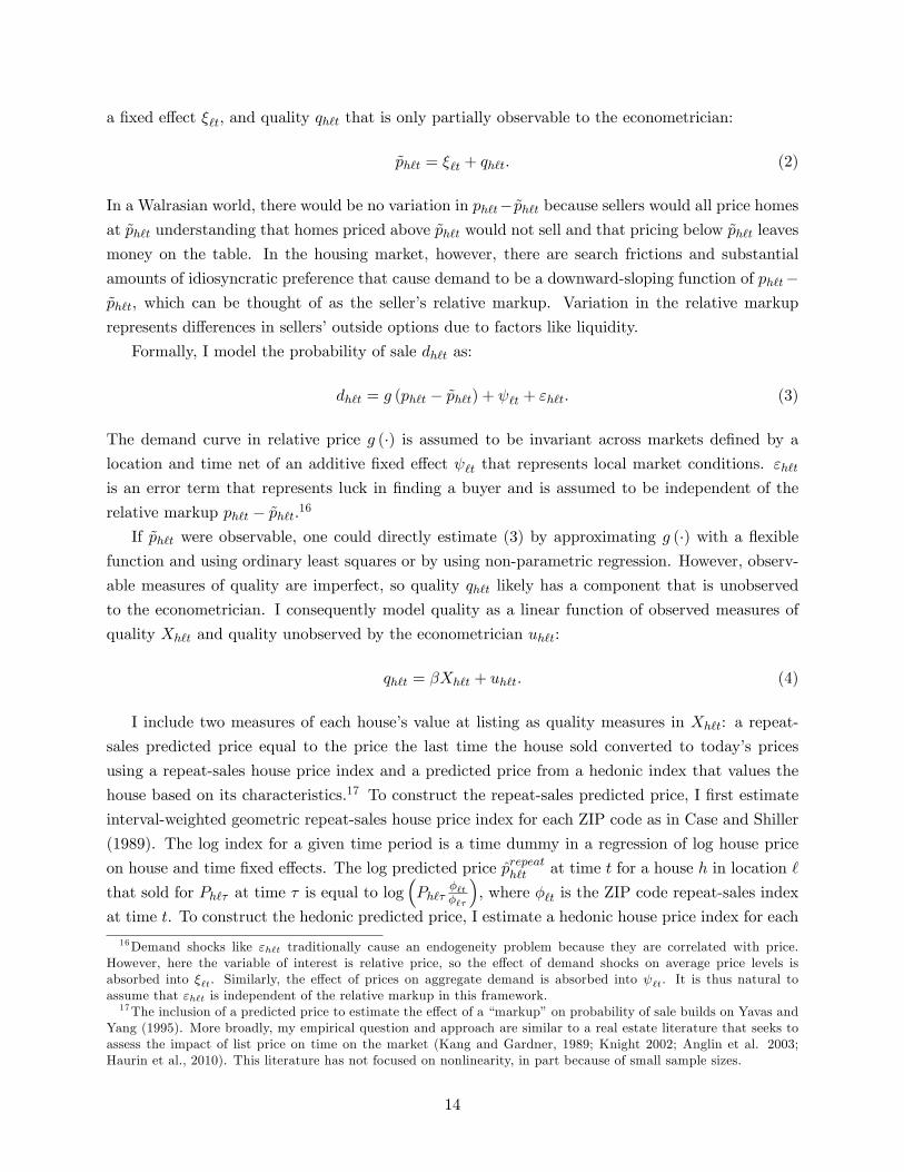
a �xed e¤ect �`t, and quality qh`t that is only partially observable to the econometrician:

~ph`t = �`t + qh`t. (2)

In a Walrasian world, there would be no variation in ph`t� ~ph`t because sellers would all price homesat ~ph`t understanding that homes priced above ~ph`t would not sell and that pricing below ~ph`t leaves

money on the table. In the housing market, however, there are search frictions and substantial

amounts of idiosyncratic preference that cause demand to be a downward-sloping function of ph`t�~ph`t, which can be thought of as the seller�s relative markup. Variation in the relative markup

represents di¤erences in sellers�outside options due to factors like liquidity.

Formally, I model the probability of sale dh`t as:

dh`t = g (ph`t � ~ph`t) + `t + "h`t. (3)

The demand curve in relative price g (�) is assumed to be invariant across markets de�ned by alocation and time net of an additive �xed e¤ect `t that represents local market conditions. "h`tis an error term that represents luck in �nding a buyer and is assumed to be independent of the

relative markup ph`t � ~ph`t.16

If ~ph`t were observable, one could directly estimate (3) by approximating g (�) with a �exiblefunction and using ordinary least squares or by using non-parametric regression. However, observ-

able measures of quality are imperfect, so quality qh`t likely has a component that is unobserved

to the econometrician. I consequently model quality as a linear function of observed measures of

quality Xh`t and quality unobserved by the econometrician uh`t:

qh`t = �Xh`t + uh`t: (4)

I include two measures of each house�s value at listing as quality measures in Xh`t: a repeat-

sales predicted price equal to the price the last time the house sold converted to today�s prices

using a repeat-sales house price index and a predicted price from a hedonic index that values the

house based on its characteristics.17 To construct the repeat-sales predicted price, I �rst estimate

interval-weighted geometric repeat-sales house price index for each ZIP code as in Case and Shiller

(1989). The log index for a given time period is a time dummy in a regression of log house price

on house and time �xed e¤ects. The log predicted price p̂repeath`t at time t for a house h in location `

that sold for Ph`� at time � is equal to log�Ph`�

�`t�`�

�, where �`t is the ZIP code repeat-sales index

at time t. To construct the hedonic predicted price, I estimate a hedonic house price index for each

16Demand shocks like "h`t traditionally cause an endogeneity problem because they are correlated with price.However, here the variable of interest is relative price, so the e¤ect of demand shocks on average price levels isabsorbed into �`t. Similarly, the e¤ect of prices on aggregate demand is absorbed into `t. It is thus natural toassume that "h`t is independent of the relative markup in this framework.17The inclusion of a predicted price to estimate the e¤ect of a �markup�on probability of sale builds on Yavas and

Yang (1995). More broadly, my empirical question and approach are similar to a real estate literature that seeks toassess the impact of list price on time on the market (Kang and Gardner, 1989; Knight 2002; Anglin et al. 2003;Haurin et al., 2010). This literature has not focused on nonlinearity, in part because of small sample sizes.

14

ZIP code using a third order polynomial in age, log square feet, bedrooms, and bathrooms for the

hedonic factor. The predicted log price p̂hedonict is the sum of a house�s hedonic value as implied

by a regression and the �xed e¤ect in the regression for a given time period. The construction of

both indices follows practices common in the literature and is detailed in Appendix A. I include

both predicted prices in Xh`t because each approach has its virtues (Meese and Wallace, 1997).18

In Appendix C, I show the results are robust to modeling quality as a more �exible function of the

predicted prices and to including other observables in Xh`t.

Combining (2) and (4), the reference price ~ph`t can be written as:

~ph`t = �`t + �Xh`t + uh`t (5)

where again �`t is a �xed e¤ect that represents the average price in location ` at time t and uh`t is

unobserved quality.

3.2.2 Instrument

To identify the demand curve g (�) in the presence of unobserved quality, I use plausibly exogenoussupply-side variation in the list price due to the liquidity needs of sellers. Sellers face a trade-o¤

between selling at a higher price and selling faster. Sellers with less liquidity and consequently a

higher marginal utility of cash on hand choose a higher list price and longer time on the market.

A proxy for liquidity that is orthogonal to unobserved quality and seller patience can is thus an

instrument for list price.

The proxy for liquidity that I use is the equity a seller extracts from their sale. Housing is a

large component of household wealth, and many sellers use the equity they extract from sale for

the down payment on their next home (Stein, 1995). This increases the marginal utility of cash

on hand for sellers who extract very little equity from their house because each additional dollar

of equity they extract can be leveraged to buy a substantially better house. The marginal utility

of cash is lower for sellers extracting substantial equity because their purchasing power is limited

more by their creditworthiness and overall budget than the cash they have on hand. Consequently,

homeowners with lower equity positions set higher list prices and sell their houses at higher prices

(Genesove and Mayer, 1997; Genesove and Mayer, 2001).

Because �nancing and re�nancing decisions make the equity of sellers endogenous, I use as

my instrument the log of appreciation in the ZIP repeat-sales house price index since purchase

zh`t = log��`t�`�

�, where � is the repeat-sales house price index, t is the period of listing, and �

is the period of previous sale.19 This would be isomorphic to equity if all homeowners took out

an identical mortgage and did not re�nance. The instrument thus compares sellers who purchase

18The hedonic approach uses a limited set of characteristics and assumes that their valuation over time is constantbecause I have only a single snapshot of characteristics, but it uses all sales. Repeat sales controls for home �xede¤ects but only uses a subset of the data and assumes that house quality is constant and that the set of housestrading at any given time is representative.19Here zh`t is a measure of liquidity, whereas when multiplied by the previous price Ph`� in Xh`t it is used to

convert the previous price to present values and constrained to have the same coe¢ cient as the previous price Ph`t.

15

identical homes with identical mortgages but who have di¤erent amounts of cash on hand to make

their next down payment because one seller�s home appreciated more in value than the other�s.

If variation in seller liquidity represented by zh`t is independent of unobserved quality and is

the only source of variation in price conditional on quality and average price, zh`t can be used as

an instrument to trace out the demand curve g (�). Because existing evidence shows that the e¤ectof equity is non-linear and strongest for sellers with low equity (Genesove and Mayer, 1997), I let

zh`t a¤ect price through a �exible function f (�). Formally, g (�) is identi�ed if:

Condition 1zh`t ?? (uh`t; "h`t)

and

ph`t = f (zh`t) + ~ph`t

= f (zh`t) + �`t + �Xh`t + uh`t. (6)

The �rst half of Condition 1 is an exclusion restriction that requires that appreciation since

purchase have no direct e¤ect on the outcome, either through fortune in �nding a buyer "h`t in

equation (3) or through unobserved quality uh`t. If this is the case, zh`t only a¤ects probability of

sale through the relative markup ph`t � ~ph`t. Because I use ZIP � quarter of listing �xed e¤ects,

the variation in zh`t comes from sellers who sell at the same time in the same market but purchased

at di¤erent points in the cycle. Condition 1 can thus be interpreted as requiring that unobserved

quality be independent of when the seller purchased.

This assumption is di¢ cult to test because I only have a few years of listings data, so �exibly

controlling for when a seller bought weakens the e¤ect of the instrument on price in equation (6)

and widens the con�dence intervals to the point that any curvature is not statistically signi�cant.

Nonetheless, I evaluate the identi�cation assumption in four ways as documented in Appendix C.

First, I vary the observable measures of quality. Second, I include including a linear time trend in

date of purchase or time since purchase. Third, I limit the sample to sellers who purchased prior to

2004 and again include a linear time trend, eliminating variation from sellers who purchased near

the peak of the bubble or during the bust. In all three cases, the results remain robust. Finally,

I show that the shape of the estimated demand curve is similar for IV and OLS, although OLS

results in a more inelastic demand curve due to the bias created by unobserved quality. While these

tests assuage some concerns, if homes with very low appreciation since purchase are of substantially

lower unobserved quality despite their higher average list price, my identi�cation strategy would

overestimate the true amount of curvature in the data.20

I focus on sellers for whom the exogenous variation is cleanest and consequently exclude three

groups. First, many individuals who have had negative appreciation since purchase are not the

20One concern is that sellers with higher appreciation since purchase improve their house in unobservable ways withtheir home equity. However, this would create a positive relationship between price and appreciation since purchasewhile I �nd a strong negative relationship.

16

claimant on the residual equity in their homes� their mortgage lender is. For these individuals,

appreciation since purchase is directly related to how far underwater they are, which in turn a¤ects

the foreclosure and short sale processes of the mortgage lender or servicer. Because I am interested

in market processes, I exclude short sales, withdrawals that are subsequently foreclosed upon,

and individuals who have had negative appreciation since purchase from the analysis. Second,

mortgage servicers and government-sponsored enterprises selling foreclosed homes have no reason

to be sensitive to the amount of appreciation since the foreclosed-upon homeowner purchased

and are dropped. Finally, investors who purchase, improve, and �ip homes typically have a low

appreciation in their ZIP code since purchase but improve the quality of the house in unobservable

ways. To minimize the e¤ect of investors, I exclude sellers who previously purchased with all cash,

a hallmark of investors.

The second part of Condition 1 requires that liquidity embodied in zh`t is the only reason for

variation in ph`t � ~ph`t. This is a strong assumption because there may be components of liquiditythat are unobserved or other reasons that homeowners list their house at a price di¤erent from

~ph`t, such as heterogeneity in discount rates. If the second part of the condition did not hold, then

the estimates would be biased because the true ph`t � ~ph`t would equal f (zh`t) + �h`t, and the

unobserved error �h`t enters g (�) nonlinearly.However, if other sources of variation in the relative markup ph`t � ~ph`t are independent of the

variation induced by the instrument, the error in ph`t � ~ph`t would not cause spurious concavity.Intuitively, noise in ph`t� ~ph`t would cause the observed probability of sale at each observed ph`t�~ph`t to be an average of the probabilities of sale at true ph`t � ~ph`ts that are on average evenly

scrambled. Consequently, although the slope may be biased, the curvature of a monotonically-

decreasing demand curve is preserved. An analytical result can be obtained if the true g (�) is acubic regression function as in Hausman et al. (1991):

Lemma 2 Consider the econometric model described by (3) and (5) and suppose that:

zh`t ?? (uh`t; "h`t) , (7)

ph`t = f (zh`t) + �h`t + ~ph`t, (8)

�h`t ?? f (zh`t), and the true regression function g (�) is a third-order polynomial. Then estimatingg (�) assuming that ph`t = f (zh`t) + ~ph`t yields the true coe¢ cients of the second- and third-order

terms in g (�).

Proof. See Appendix C.While a special case, Lemma 2 makes clear that the bias in the estimated concavity is minimal if

�h`t ?? f (zh`t). Appendix C.5 shows more generally using Monte Carlo simulation that if �h`t ??f (zh`t), the degree of concavity is if anything under-estimated.

However, spurious concavity is possible if other sources of variation in the relative markup are

correlated with the instrument. Speci�cally, Appendix C.5 presents Monte Carlo simulations that

17

show that if the instrument captures most of the variation in the relative markup ph`t� ~ph`t at lowlevels of appreciation since purchase but very little of the variation at high levels of appreciation

since purchase, spurious concavity is generated because the slope is attenuated for low relative

markups but not high relative markups. However, quantitatively an extreme amount of unobserved

variation in the relative markup ph`t � ~ph`t is necessary to spuriously generate the amount of

concavity in the data.

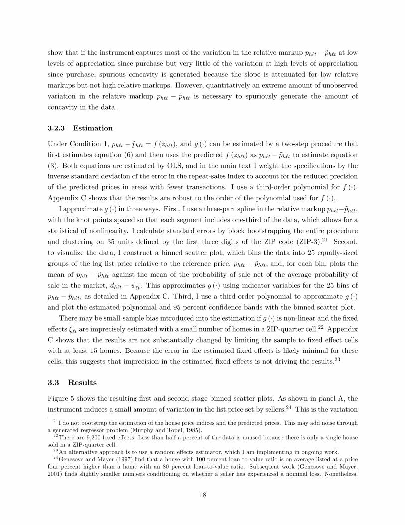
3.2.3 Estimation

Under Condition 1, ph`t � ~ph`t = f (zh`t), and g (�) can be estimated by a two-step procedure that�rst estimates equation (6) and then uses the predicted f (zh`t) as ph`t � ~ph`t to estimate equation(3). Both equations are estimated by OLS, and in the main text I weight the speci�cations by the

inverse standard deviation of the error in the repeat-sales index to account for the reduced precision

of the predicted prices in areas with fewer transactions. I use a third-order polynomial for f (�).Appendix C shows that the results are robust to the order of the polynomial used for f (�).

I approximate g (�) in three ways. First, I use a three-part spline in the relative markup ph`t�~ph`t,with the knot points spaced so that each segment includes one-third of the data, which allows for a

statistical of nonlinearity. I calculate standard errors by block bootstrapping the entire procedure

and clustering on 35 units de�ned by the �rst three digits of the ZIP code (ZIP-3).21 Second,

to visualize the data, I construct a binned scatter plot, which bins the data into 25 equally-sized

groups of the log list price relative to the reference price, ph`t � ~ph`t, and, for each bin, plots themean of ph`t � ~ph`t against the mean of the probability of sale net of the average probability of

sale in the market, dh`t � `t. This approximates g (�) using indicator variables for the 25 bins ofph`t � ~ph`t; as detailed in Appendix C. Third, I use a third-order polynomial to approximate g (�)and plot the estimated polynomial and 95 percent con�dence bands with the binned scatter plot.

There may be small-sample bias introduced into the estimation if g (�) is non-linear and the �xede¤ects �`t are imprecisely estimated with a small number of homes in a ZIP-quarter cell.

22 Appendix

C shows that the results are not substantially changed by limiting the sample to �xed e¤ect cells

with at least 15 homes. Because the error in the estimated �xed e¤ects is likely minimal for these

cells, this suggests that imprecision in the estimated �xed e¤ects is not driving the results.23

3.3 Results

Figure 5 shows the resulting �rst and second stage binned scatter plots. As shown in panel A, the

instrument induces a small amount of variation in the list price set by sellers.24 This is the variation

21 I do not bootstrap the estimation of the house price indices and the predicted prices. This may add noise througha generated regressor problem (Murphy and Topel, 1985).22There are 9,200 �xed e¤ects. Less than half a percent of the data is unused because there is only a single house

sold in a ZIP-quarter cell.23An alternative approach is to use a random e¤ects estimator, which I am implementing in ongoing work.24Genesove and Mayer (1997) �nd that a house with 100 percent loan-to-value ratio is on average listed at a price

four percent higher than a home with an 80 percent loan-to-value ratio. Subsequent work (Genesove and Mayer,2001) �nds slightly smaller numbers conditioning on whether a seller has experienced a nominal loss. Nonetheless,

18

Figure 5: Instrumental Variable Estimates of the E¤ect of List Price on Probability of Sale

Notes: Panel B shows a binned scatter plot of the probability of sale within 13 weeks net of �xed e¤ects (with the average

probability of sale within 13 weeks added in) against the estimated log relative markup p� ~p. It also shows an overlaid cubic�t of the relationship, as in equation (3). To create the �gure, a �rst stage regression of the log list price on a third-order

polynomial in the instrument, �xed e¤ects at the ZIP x �rst quarter of listing level, and repeat sales and hedonic log predicted

prices, as in (6), is estimated by OLS. The predicted value of the polynomial of the instrument is used as the relative markup.

The �gure splits the data into 25 equally-sized bins of this estimated relative markup and plots the mean of the estimated

relative markup against the mean of the probability of sale within 13 weeks net of �xed e¤ects for each bin, as detailed in

Appendix C. Before binning, the 1st and 99th percentiles of the log sale price residual and any observations fully absorbed

by �xed e¤ects are dropped. The entire procedure is weighted by the reciprocal of the standard deviation of the prediction

error in the repeat-sales house price index in the observation�s ZIP code from 1988 to 2013. The sample is limited to the

IV subsample of homes that are not sales of foreclosures or short sales, sales of homes with negative appreciation since the

seller purchased, or sales by investors who previously purchased with all cash. The grey bands indicate a pointwise 95-percent

con�dence interval for the cubic �t created by block bootstrapping the entire procedure on 35 ZIP-3 clusters. Panel A shows

the �rst stage relationship between the instrument and log initial list price in equation (6) by residualizing the instrument and

the log initial list price against the two predicted prices and �xed e¤ects, binning the data into 25 equally-sized bins of the

instrument residual, and plotting the mean of the instrument residual against the mean of the log initial list price residual for

each bin. N = 111,293 observations prior to dropping the 1st and 99th percentiles and unique zip-quarter cells.

I use to identify the shape of demand. The �rst stage is strong with a joint F statistic for the third

order polynomial of the instrument in (6) of 128. Panel B shows that a clear concave relationship

is visible in the second stage, with very inelastic demand for relatively low priced homes and elastic

demand for relatively high priced homes. This curvature is also visible in the cubic polynomial

�t.25 Table 3 shows regression results when g (�) is approximated by a three-part spline. Panel Bshows the IV results. The concavity visible in Figure 5 is apparent, with the highest tercile having

the similarity between their four percent �gure and the amount of variation induced by the instrument in my �rststage is reassuring.25Most of the curvature comes from the top quarter of the sample because the instrument has the largest e¤ect on

the small number of sellers with low appreciation since purchase and a smaller e¤ect on sellers who have experiencemoderate to high appreciation.

19

Table 3: The E¤ect of List Price on Probability of Sale: Regression Results

Panel A: Ordinary Least SquaresDependent Var: Sell Within 13 Weeks

Sample: All Listings With Prior Observation(431,830 obs, 420,820 After Dropping 1st and 99th % and Cells With One Obs)

Controls: ZIP � Quarter � Distress FE, Repeat and Hedonic Predicted PriceLowest Tercile Middle Tercile Highest Tercile High - Low

Coe¢ cient on List Price 0.161*** -0.500*** -0.483*** -0.643***Residual Spline (0.031) (0.091) (0.039) (0.056)

Bootstrapped 95% CI [-0.767,-0.555]

Panel B: Instrumental VariableDependent Var: Sell Within 13 Weeks

Sample: Listings With Prior Obs, excluding REO, Short Sales, Investors, Neg Appreciation

(111,293 obs,108,696 After Dropping 1st and 99th % and Cells With One Obs)Controls: ZIP � Quarter FE, Repeat and Hedonic Predicted PriceInstrument: Appreciation Since Purchase

Lowest Tercile Middle Tercile Highest Tercile High - LowCoe¢ cient on List Price -0.320 0.261 -2.327*** -2.007***

Residual Spline (0.334) (1.651) (0.616) (0.588)Bootstrapped 95% CI [-3.577,-1.293]

Notes: * p < 0.05, ** p<0.01, *** p<0.001. Each row shows regression coe¢ cients when g(.) in equation (3) is approximated

using a three-segment linear spline with an equal fraction of the data in each segment. This relationship represents the e¤ect of

the log relative markup on the probability of sale within 13 weeks. In the IV panel, a �rst stage regression of log list price on

a third-order polynomial in the instrument, �xed e¤ects at the ZIP x �rst quarter of listing level, and log predicted price using

both a repeat-sales and a hedonic methodology, as in (6) is estimated by OLS. The predicted value of the polynomial of the

instrument is used as the relative markup in equation (3), which is estimated by OLS. The sample is restricted to non-REOs,

non-short sales, properties with positive appreciation since purchase, and properties not previously purchased with all cash

(investors). In the OLS panel, quality is assumed to be perfectly measured by the hedonic and repeat-sales predicted prices and

have no unobserved component. OLS thus regresses log list price on �xed e¤ects and the predicted prices and uses the residual

as the estimated relative markup into equation (3), as described in Appendix C. OLS uses the full set of listings with a previous

observed transaction, so to prevent distressed sales from biasing the results, the �xed e¤ects are at the quarter of initial listing

x ZIP x distress status level. Distress status corresponds to three groups: normal sales, REOs (sales of foreclosed homes and

foreclosure auctions), and short sales (cases where the transaction price is less than the amount outstanding on the loan and

withdrawals that are subsequently foreclosed on in the next two years). Both procedures are weighted by the reciprocal of

the standard deviation of the prediction error in the repeat-sales house price index in the observation�s ZIP code from 1988 to

2013. Before creating the spline, the 99th and 1st percentiles of the relative markup are dropped, as are any observations fully

absorbed by �xed e¤ects. In addition to the regression coe¢ cients, the di¤erence between the highest and lowest tercile of the

spline is reported. Standard errors and the 95 percent con�dence interval for the di¤erence between the �rst and third terciles

are computed by block bootstrapping the entire procedure on 35 ZIP-3 clusters.

a slope that is seven times the lowest tercile. The di¤erence between the highest and lowest tercile

slopes is statistically signi�cant.

As a point of comparison, Panel A shows OLS results for the full sample of homes with a prior

20

observed transaction. The �xed e¤ects are at the ZIP � quarter � REO seller � short seller level toprevent distressed sales from biasing the results. OLS assumes away unobserved quality and should

be positively biased if ~ph`t is positively correlated with ph`t due to omitted unobserved quality. This

is the case: the estimated demand curve is more elastic for IV than OLS. In fact, the OLS bias is

strong enough that the demand curve slopes signi�cantly upward in the lowest tercile. Nonetheless,

a clear pattern of concavity is apparent in the OLS results. Appendix C shows that OLS looks

similar on the limited IV sample.

The highest tercile IV estimates imply that raising one�s price by one percent reduces the

probability of sale within 13 weeks by approximately 2.3 percentage points on a base of 46.8

percentage points, a reduction of 5 percent. This corresponds to a one percent price hike increasing

the time to sale by six to eleven days. This �gure is of comparable magnitude to Carrillo (2012),

who estimates a structural search model of the steady state of the housing market with multiple

dimensions of heterogeneity using data from Charlottesville, Virginia from 2000 to 2002. Although

we use very di¤erent empirical approaches, in a counterfactual simulation, he �nds that a one

percent list price increase increases time on the market by a week, while a �ve percent list price

increase increases time on the market by a year. Carrillo also �nds small reductions in time on the

market from underpricing, consistent with the nonlinear relationship found here.

Appendix C shows that the results are robust across geographies, time periods, and speci�ca-

tions, although in some cases restricting to a smaller sample leads to insigni�cant results. It also

shows that concavity is clearly visible in the reduced-form relationship between the instrument and

probability of sale. Finally, the Appendix shows the results are robust to other measures of quality

and to using transaction prices rather than using list prices. The instrumental variable results thus

provide evidence of demand concave in relative price for these three MSAs from 2008 to 2013.26

4 A Model of House Price Momentum

This section introduces an equilibrium search model with concave demand. The model includes two

additional ingredients new to the housing search literature. First, because concave demand only

ampli�es existing price insensitivity, I introduce variants of the model with two separate sources

of insensitivity: staggered pricing as in Taylor (1980) and a small number of backward-looking

rule-of-thumb sellers as in Haltiwanger and Waldman (1989) and Gali and Gertler (1999).

Second, I include an endogenous entry decision for buyers and sellers so that the same model

can be used to assess how the re-timing of purchases and sales in light of momentum a¤ects housing

dynamics. Entry is a form of intertemporal arbitrage that reduces the amount of momentum in the

model, and with a completely elastic entry margin momentum would be eliminated (Barsky et al.,

2007). Consequently, the model features some households who have to move immediately so that

the entry margin is important but not strong enough to eliminate momentum.

26Aside from the tail end of my sample, this period was a depressed market. The similarity between my resultsand Carrillo�s provide some reassurance that the results I �nd are not speci�c to the time period, but I cannot ruleout that the nonlinearity would look di¤erent in a booming market.

21

Table 4: Notation in the Model

Variable Description NoteMasses

Pop Total Population (Housing Stock Mass One)B Endogenous Mass of Buyers Value Fn V b

S Endogenous Mass of Sellers Value Fn V s

R Endogenous Mass of Renters Value Fn V r

H Endogenous Mass of Homeowners Value Fn V h

Flow Utilitiesb Flow Utility of Buyer (Includes search cost)s Flow Utility of Seller (includes search cost)u Flow Utility of Renter Shocked Variableh Flow Utility of Homeowner

Moving Shock Probabilities

�h Prob Homeowner Gets Shock�r Prob Renter Gets Shock

Costsc Stochastic Cost for Homeowner to Stay in Home � C (c) ; U (c; �c)k Stochastic Cost for Renter to Stay Renter (Negative) � K (k) ; U

�k; �k�

c� Threshold c Above Which Homeowners Enter Endogenousk� Threshold k Above Which Renters Enter Endogenous

Other Parameters� Discount FactorL Probability Seller Leaves Metro AreaV 0 Value Realized Upon Exiting Metro Area

The model builds on search models of the housing market, such as Wheaton (1990), Krainer

(2001), Novy-Marx (2009), Piazzesi and Schneider (2009), Caplin and Leahy (2011), Genesove and

Han (2012), Head et al. (2014), Ngai and Tenreyro (2013), Burnside et al. (2013), and Diaz and

Jerez (2013). I also incorporate ideas from models with price posting with undirected search (e.g.,

Kudoh, 2013).

I �rst introduce a framework that models a metropolitan area with a �xed population and

housing stock. I then describe the housing market component and show how sellers set list prices.

I then introduce staggered pricing and rule-of-thumb consumers. The notation used in the model

is summarized in Tables 4 and 5.

4.1 Setting

Time is discrete and all agents are risk neutral. Agents have a discount factor of � and time t is

denoted with a subscript. There is a �xed housing stock of mass one, no construction, and a �xed

22

population of size Pop.27 Each period occurs in three stages: �rst search and transactions occur,

then �ow utilities are realized, and �nally mismatch shocks occur.

There are four types of homogenous agents: a mass Bt of buyers, St of sellers, Ht of homeowners,

and Rt of renters. These agents have �ow utilities (inclusive of search costs) b, s, h, and r, and

value functions V bt , Vst , V

ht , and V

rt , respectively. Buyers and sellers are active in the housing

market, which is described in the next section. The rental market, which serves as a reservoir of

potential buyers, is unmodeled aside from the �ow utility net of rents. I assume that each agent

can own only one home, which precludes short sales and investor-owners, although I allow for the

re-timing of buyer and seller entry decisions described below.

Each period with probability �h and �r, respectively, homeowners and renters receive shocks

that cause them to separate from their current house or apartment, as in Wheaton (1990). However,

rather than automatically entering the housing market, the shocks cause homeowners and renters

to draw a one-time cost, c � C (�) for homeowners and k � K (�) (likely negative) for renters,that can be paid to stay in their current house or apartment and receive the same �ow utility as

before instead of moving. Because the seller entry elasticity appears to be constant over the cycle

as shown in Appendix E, the cost distributions are parameterized as uniform: c � U (c; �c) and

k � U�k; �k�. This setup captures that potential movers have heterogeneous reasons to buy or sell

and consequently di¤er in the ease with which they can re-time their transaction.

A renter who decides not to pay the cost k enters the market as a homogenous buyer. A

homeowner who decides not to pay the cost c learns after making their entry decision whether they

leave the MSA with probability L, in which case they become a seller and receive termination payo¤

V 0 for leaving, or whether they remain in the city with probability 1�L. If they remain in the city,they simultaneously become a buyer and a homogenous seller. These two roles are assumed to be

quasi-independent so that the value functions do not interact and no structure is put on whether

agents buy or sell �rst, as in Ngai and Tenreyro (2013) and Guren and McQuade (2013).

A homeowner who draws a cost c enters the market if:

c � V ht � V st � LV 0 � (1� L)V ht � c�t . (9)

Similarly a renter enters if

k � V rt � V bt � k�t . (10)

The cuto¤s c�t and k�t determine the marginal buyer and seller and control their �ow into the

market.28

Because the population is constant, every time a seller leaves the city they are replaced by

a new entrant. Entrants draw a cost of being a renter and decide whether to rent or buy in

27Construction is omitted for parsimony. The model best applies to areas with inelastic housing supply in whichmomentum is stronger, although it is also relevant to the short run in elastically supplied metro areas, in whichmomentum is weaker but still important. See Head et al. (2014) for a model with a construction margin.28This setup makes two implicit assumptions for tractability. First, although individuals are heterogeneous in their

motivation to move, once they enter the market they are homogenous. Second, if an individual decides not to movetoday, they do not make another decision about moving until they get another shock.

23

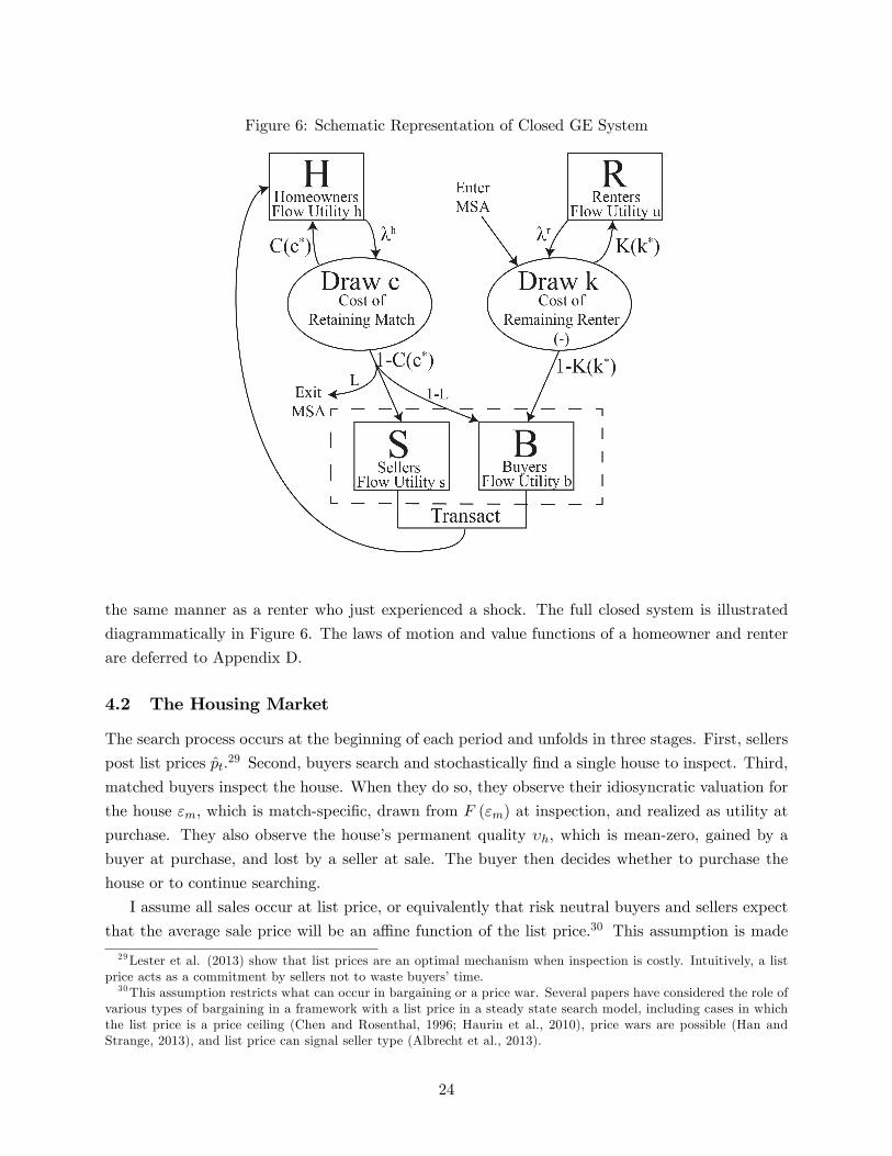
Figure 6: Schematic Representation of Closed GE System

the same manner as a renter who just experienced a shock. The full closed system is illustrated

diagrammatically in Figure 6. The laws of motion and value functions of a homeowner and renter

are deferred to Appendix D.

4.2 The Housing Market

The search process occurs at the beginning of each period and unfolds in three stages. First, sellers

post list prices p̂t.29 Second, buyers search and stochastically �nd a single house to inspect. Third,

matched buyers inspect the house. When they do so, they observe their idiosyncratic valuation for

the house "m, which is match-speci�c, drawn from F ("m) at inspection, and realized as utility at

purchase. They also observe the house�s permanent quality �h, which is mean-zero, gained by a

buyer at purchase, and lost by a seller at sale. The buyer then decides whether to purchase the

house or to continue searching.

I assume all sales occur at list price, or equivalently that risk neutral buyers and sellers expect

that the average sale price will be an a¢ ne function of the list price.30 This assumption is made

29Lester et al. (2013) show that list prices are an optimal mechanism when inspection is costly. Intuitively, a listprice acts as a commitment by sellers not to waste buyers�time.30This assumption restricts what can occur in bargaining or a price war. Several papers have considered the role of

various types of bargaining in a framework with a list price in a steady state search model, including cases in whichthe list price is a price ceiling (Chen and Rosenthal, 1996; Haurin et al., 2010), price wars are possible (Han andStrange, 2013), and list price can signal seller type (Albrecht et al., 2013).

24

Table 5: Notation in Housing Market

Variable Description NoteUtilities

"m Match-Speci�c One-Time Utility Bene�t � F (")�h Permanent House Quality Mean Zero

Stochastic Draws�h;t Noise in Observed �h, IID Common in Period t � G (�)

Parameters / Values� Market Tightness = B=S Endogenous~� E¤ective Market Tightness = B=Svisited Endogenous

q�~��

Prob. Seller Meets Buyer (Matching Function) Endogenous

� Constant in Matching Function Matching Function Elasticity Distribution of Prices Endogenous"� Threshold "m for Purchase Endogenous� Threshold for Binary Signal

Distribution Parameters� Exponential Dist Param for F (")� Logistic Variance Param for G (�)

for tractability and is not essential to the propagation mechanism. It is also less strong than it

may �rst appear: although many houses do sell above or below list price, Appendix A.3 shows that

in the merged Altos-DataQuick micro data, the modal transaction price is the list price, and the

average and median di¤erences between the list and transaction price are less than 0.01 log points

and do not vary much across years.31

Buyer search for homes is partially directed in that buyers search only for homes that do not

appear overpriced for their quality, but whether a house is overpriced for its quality is noisily

observed. This directs search away from overpriced homes but preserves much of the structure of

random search in which frictions prevent buyers from seeking out the lowest price house relative to

quality or the house with which they have the best match. Formally, after prices are posted, buyers

receive a binary signal from their real estate agent or from advertisements. The signal reveals

whether a house�s quality-adjusted price relative to the average quality-adjusted price is above a

threshold. However, quality �h (or equivalently the observation of the average price) is subject to

mean zero noise �h;t � G (�), where G (�) is assumed to be constant over time. This noise, whichrepresents how well a house is marketed in a given period, is common to all buyers but independent

and identically distributed across periods.

Buyers can inspect at most one home per period, and although they can limit their search set, it

31An important feature of the housing market is that most price changes are decreases. Consequently, the di¤erencebetween the initial list price and the sale price �uctuates substantially over the cycle as homes that do not sell cuttheir list price. I abstract from such duration dependence to maintain a tractable state space.

25

is assumed that once they do so they search randomly among homes in their search set and cannot

direct their search to a particular type of home. Buyers who only observe this signal before choosing

their search optimally limit their search to homes that the signal indicates are not overpriced.32

These are homes for which the quality-adjusted price pt � p̂t � �h satis�es,

pt � �h;t � E [pt] � �, (11)

where is the distribution of prices. Because the signal reveals nothing else about the home, buyers

cannot do better than searching randomly within homes satisfying (11). I assume that search

occurs according a constant returns to scale matching function so that the number of matches

can be written as a function of the number of buyers and visited sellers m�Bt; S

visitedt

�. Because

m is constant returns to scale, I rewrite m as a function q�~�t

�of the ratio of buyers to visited

sellers ~�t = BtSvisitedt

= BtStE[1�G(pt�E[pt]��)] . The matching function captures frictions in the search

process that prevent all reasonably-priced homes and all buyers from having an inspection each

period. For instance, buyers randomly allocating themselves across houses may miss a few houses,

or there may not be a mutually-agreeable time for a buyer to visit a house in a given period.

After inspecting a house, buyers purchase if their surplus from doing so V ht + "m � p� b� �V btis positive. This leads to a threshold rule to buy if "m > pt+ b+�V

bt+1�V ht � "�t and a probability

of purchase given inspection of 1� F ("�t ).33

Sellers have rational expectations but set their list price before �h;t is realized and without

knowing the valuation of the particular buyer who visits their house. The demand curve they

face when they set their price, d�pt;t; ~�t

�, is the ex-ante probability of sale for a house with a

list price pt given a distribution of list prices t and functional market tightness ~�t. d (pt;t; �t)

can be written as the product of the probability the house satis�es (11) and is searched, 1 �G (pt � E [pt]� �), the probability a house that is searched matches with a buyer, q

�~�t

�, and the

probability of purchase given inspection, 1� F ("�t ):

d�pt;t; ~�t

�= q

�~�t

�(1�G (pt � E [pt]� �)) (1� F ("�t )) . (12)

I parameterize the model by assuming distributions for F (�) and G (�). Speci�cally, I assumethat F ("m) is an exponential distribution with parameter � and G

��h;t�is logistic with mean

zero and variance �2 �2

3 .34 I also assume that the matching function is Cobb-Douglas q (�) = ��� ,

as is standard in the search literature. While these assumptions matter for precise quantitative

predictions of the model, they are not necessary for the intuitions it illustrates.

32This behavior is optimal if only the signal is observed. If both the signal and price are observed, one can always�nd a prior distribution for quality such that following the signal is optimal.33Because the signal reveals no information about the house�s quality �h, posted price p̂t, or match quality "m, the

search and inspection stages are independent.34 It is useful to work with distributions for which the hazard rate f

1�F and mean excess function E [x� x�jx > x�]have closed-form analytic solutions. The exponential distribution is particularly convenient because it has a singleparameter, changes in the tail density do not drive the results, and the hazard and mean excess functions are constant,although using a Weibull or Gamma yields similar results.

26

Figure 7: The Concave Demand Curve in the Model

1

Prob InspectP

rob 

Insp

ect

Relative Price1

Prob Buy |  Inspect

Pro

b B

uy | 

Insp

ect

Relative Price

1

Demand Curve

Pro

b S

ell

Relative Price1

Additive Markup

Relative Price

Add

itive

 Mar

kup

Notes: The �gures are generated using calibration described in Section 5. All probabilities and the additive markup are

calculated assuming all other sellers are setting the steady state price and considering the e¤ect of a unilateral deviation.

This setup leads to a concave demand curve with considerable curvature in the neighborhood

of the average price. At above average prices, the demand curve is dominated by whether buyers

include the house in their search set, creating an elastic demand curve. At below average prices,

buyers include the house in their search set with high probability and the demand curve is dominated

by purchase decisions based on a trade-o¤ between idiosyncratic match quality "m and price, so

demand is less elastic. To illustrate this, Figure 7 shows the shapes of the probability of inspection

q (�t) (1�G (pt � E [pt]� �)), the probability of purchase conditional on inspection 1 � F ("�t ),

and the overall demand curve d (pt;t; �t), equal to the product of the �rst two panels. (Note that

the axes are swapped from the traditional Marshallian supply and demand diagram in order to be

consistent with the empirical analysis in Section 3.)

4.3 Flexible Price Setting

If sellers can update their list price each period, the buyer and seller value functions are equal

to the value of not transacting and remaining in the market next period plus the probability of

27

purchase or sale times the party�s surplus from the transaction relative to remaining in the market.

Mathematically,

V bt = b+ �V bt+1 +d�pt;t; ~�

��t

hV ht + "

�t + E ["m � "�t j"m > "�t ]� p� b� �V bt+1

i= b+ �V bt+1 +

d�pt;t; ~�t

���t

(13)

V st = s+ �V st+1 +maxpt

nd�pt;t; ~�t

� �pt � s� �V st+1

�o; (14)

where (13) follows from the memoryless property of the exponential distribution for "m. Seller

optimization implies:

Lemma 3 The seller�s optimal list price when prices can be set �exibly each period is:

p = s+ �V st+1 +1

f("�t )1�F ("�t )

+ g(pt�E[pt]��)1�G(pt�E[pt]��)

(15)

= s+ �V st+11

1�

1

1+exp�� pt�E[pt]��

�

� + �; (16)

where the second line imposes the distributional assumptions. In a rational expectations equilibrium

pt = E [pt]. The optimal list price is unique on an interval bounded away from p =1.

Proof. See Appendix D.2.Sellers have monopoly power due to costly search. The optimal pricing problem they solve

is the same as that of a monopolist facing the demand curve d except that the marginal cost is

replaced by the seller�s outside option of searching again next period. The optimal pricing strategy

is a markup over the outside option s+�V st+1. In equation (15) it is written as an additive markup

equal to the reciprocal of the semi-elasticity of demand, �d(pt;t;�t)@d(pt;t;�t)@pt

. The semi-elasticity, in turn,

is equal to the sum of the hazard rates of the idiosyncratic preference distribution F (�) and thedistribution of signal noise G (�).

This creates a strategic complementarity in price setting because the optimal price depends

on relative price pt �E [pt] through the hazard rate of the signal G (�). In particular, the elasticityof demand rises as relative price increases, causing the optimal markup to fall from 1

� to1

1�+�,

as illustrated in Figure 7. The markup thus pushes sellers to set prices close to those of others.

However, in a rational expectations equilibrium without additional sources of price insensitivity, all

sellers choose the same list price and pt = E [pt], so there is no relative price to a¤ect the markup.

A shock to home values thus causes list price to jump proportionally to the seller�s outside option.

Consequently, I introduce variants of the model with two di¤erent sources of insensitivity of prices

to generate some initial momentum.

28

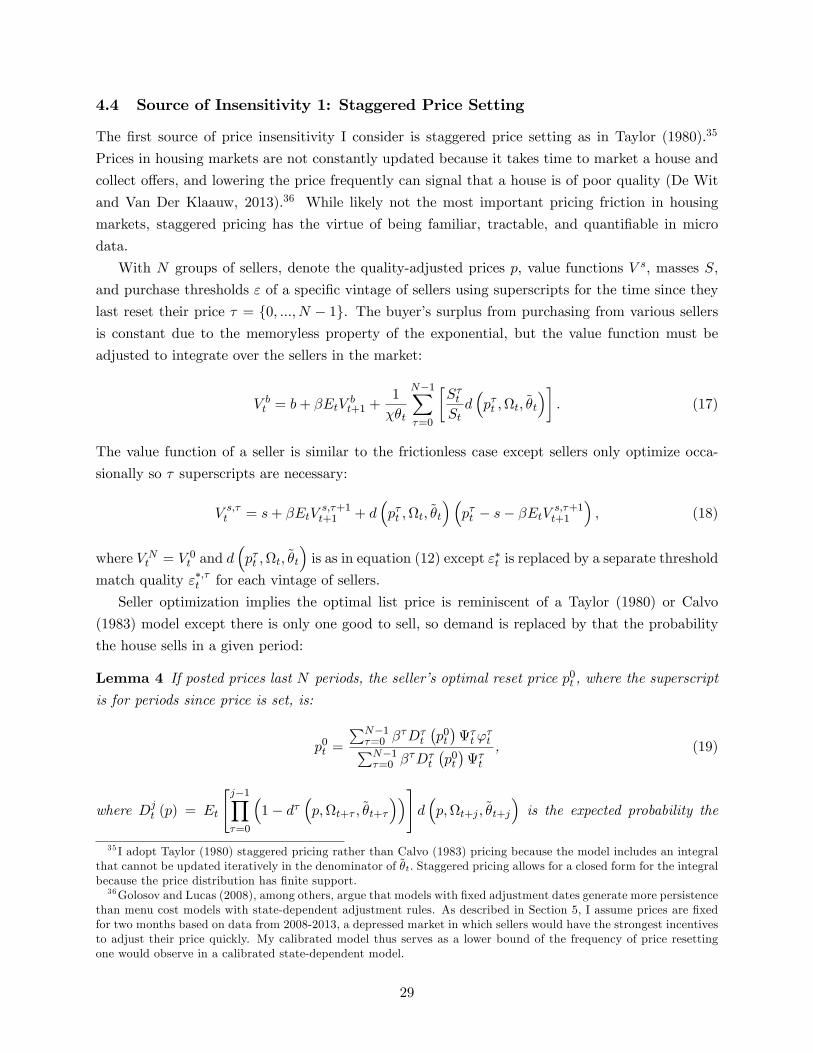
4.4 Source of Insensitivity 1: Staggered Price Setting

The �rst source of price insensitivity I consider is staggered price setting as in Taylor (1980).35

Prices in housing markets are not constantly updated because it takes time to market a house and

collect o¤ers, and lowering the price frequently can signal that a house is of poor quality (De Wit

and Van Der Klaauw, 2013).36 While likely not the most important pricing friction in housing

markets, staggered pricing has the virtue of being familiar, tractable, and quanti�able in micro

data.

With N groups of sellers, denote the quality-adjusted prices p, value functions V s, masses S,

and purchase thresholds " of a speci�c vintage of sellers using superscripts for the time since they

last reset their price � = f0; :::; N � 1g. The buyer�s surplus from purchasing from various sellers

is constant due to the memoryless property of the exponential, but the value function must be

adjusted to integrate over the sellers in the market:

V bt = b+ �EtVbt+1 +

1

��t

N�1X�=0

�S�tStd�p�t ;t;

~�t

��. (17)

The value function of a seller is similar to the frictionless case except sellers only optimize occa-

sionally so � superscripts are necessary:

V s;�t = s+ �EtVs;�+1t+1 + d

�p�t ;t;

~�t

��p�t � s� �EtV

s;�+1t+1

�; (18)

where V Nt = V 0t and d�p�t ;t;

~�t

�is as in equation (12) except "�t is replaced by a separate threshold

match quality "�;�t for each vintage of sellers.

Seller optimization implies the optimal list price is reminiscent of a Taylor (1980) or Calvo

(1983) model except there is only one good to sell, so demand is replaced by that the probability

the house sells in a given period:

Lemma 4 If posted prices last N periods, the seller�s optimal reset price p0t , where the superscript

is for periods since price is set, is:

p0t =

PN�1�=0 �

�D�t

�p0t��t'

�tPN�1

�=0 ��D�

t

�p0t��t

, (19)

where Djt (p) = Et

"j�1Y�=0

�1� d�

�p;t+� ; ~�t+�

��#d�p;t+j ; ~�t+j

�is the expected probability the

35 I adopt Taylor (1980) staggered pricing rather than Calvo (1983) pricing because the model includes an integralthat cannot be updated iteratively in the denominator of ~�t: Staggered pricing allows for a closed form for the integralbecause the price distribution has �nite support.36Golosov and Lucas (2008), among others, argue that models with �xed adjustment dates generate more persistence

than menu cost models with state-dependent adjustment rules. As described in Section 5, I assume prices are �xedfor two months based on data from 2008-2013, a depressed market in which sellers would have the strongest incentivesto adjust their price quickly. My calibrated model thus serves as a lower bound of the frequency of price resettingone would observe in a calibrated state-dependent model.

29

house is sold � periods after the price is set, �t = Et

"� @d(pt;t+� ;~�t+� )

@pt

d(pt;t+� ;~�t+�)

#is the semi-elasticity of

demand with respect to price, '�t = s+EtVs;�+1t+�+1 +

1�tis the expected optimal �exible reset price �

periods after the price is set given the expected price distribution in that period, and V s;Nt+N = V s;0t+N .

The optimal list price is unique on an interval bounded away from p = 1 given a condition in

Appendix D.2, which holds for all simulations considered.

Proof. See Appendix D.2.As is standard in staggered price models, the optimal price is a weighted average of the optimal

�exible prices that are expected to prevail on the equilibrium path until the seller can reset his or

her price. The weight put on the optimal �exible price in period t + � is equal to the discounted

probability of sale in period i times the semi-elasticity of demand in period i. Intuitively, the seller

cares more about periods in which probability of sale is higher but also about periods in which

demand is more elastic because perturbing price has a larger e¤ect on pro�t.

In equilibrium, all agents behave optimally given the search technology, the noisy signal of

relative price, and buyers�draw of their idiosyncratic taste when they visit a home. Laws of motion

apply due to the law of large numbers. I restrict attention to symmetric equilibria. A staggered

pricing equilibrium is consequently de�ned by:

De�nition 5 Equilibrium with N staggered groups of list-price-setting sellers is a set of prices p�t ,

demands d (p�t ;; �), purchase cuto¤s "�;�t , and seller value functions V s;�t for each group of sellers

� = f0; :::; N � 1g, buyer, homeowner, and renter value functions V bt , V ht , and V rt , entry cuto¤s c�tand k�t , and stocks of each type of agent Bt, S

�t � = f0; :::; N � 1g, Ht, and Rt satisfying:

1. Optimal reset pricing (19) and �xed pricing for non-resetters p�t = p��1t�1 8 � > 0

2. Optimal purchasing decisions by buyers: "�;�t = p�t + b+ �Vbt+1 � V ht

3. The demand curve for each type of seller arising from optimal buyer search given the binary

signal (12)

4. Optimal entry decisions by homeowners and renters who receive shocks (9) and (10)

5. The value functions for buyers (17) and each vintage of sellers (18) as well as for renters and

homeowners de�ned in Appendix D

6. The laws of motion for all agents de�ned in Appendix D.

Appendix D shows that the model has a unique steady state that is equivalent to the frictionless

case without staggered pricing (N = 1). A frictionless equilibrium is formally de�ned in the

Appendix D.

I add a stochastic shock process to both this model and the analogous rule-of-thumb variant

de�ned subsequently to examine their dynamic implications. The propagation mechanism for mo-

mentum does not qualitatively depend on any particular shock. However, the positive correlation

30

between price and volume in the data implies that demand-side shocks dominate.37 Although the

particular type of demand shock introduced to the model is not important for the results, I use a

shock to the �ow utility of being a renter u that changes the relative value of homeownership for

potential entrants. This takes a cue from Wheaton and Lee (2009), who show that changes in the

frequency of transitions between renting and owning due to credit conditions are a precipitating

shock for housing cycles. An example of such a shock would be a change in credit standards for

new homeowners. I implement the shock by assuming that u = �u+x, where x is an AR(1) process

understood by the forward-looking agents:

xt = �xt�1 + � and � � N�0; �2�

�. (20)

The model cannot be solved analytically, so I simulate it numerically using a log-cubic approx-

imation pruning higher order terms as in Kim et al. (2008) implemented in Dynare (Adjemian et

al., 2013). Appendix F shows that the impulse responses are similar in an exactly-solved model

with a permanent and unexpected shock.

4.5 Source of Insensitivity 2: A Small Fraction of Rule-of-Thumb Sellers

The second source of price insensitivity I consider is a small fraction of rule-of-thumb sellers. Since

Case and Shiller (1987), sellers with backward-looking expectations have been thought to play

an important role in housing markets. Previous models assume that all agents have backward-

looking beliefs (e.g., Berkovec and Goodman, 1996), but some observers have found the notion

that the majority of sellers are non-rational unpalatable given the �nancial importance of housing

transactions for many households. Some fraction of sellers, however, may not �nd it worthwhile to

scrutinize current market conditions due to information costs, and my model only requires a handful

of backward-looking sellers because of the strategic complementarity. Consequently, I introduce a

small number of rule-of-thumb sellers, as in Campbell and Mankiw (1989), and assess quantitatively

what fraction of sellers is needed to be non-rational to explain the momentum in data, similar to

Gali and Gertler (1999).

I assume that at all times a fraction 1� � of sellers set their list price pRt rationally according

to Lemma 3 and (15) but a fraction � of sellers uses a backward-looking rule of thumb to set their

list price pNt .

The backward-looking sellers are near-rational sellers whose optimizing behavior produces a

price-setting rule of thumb based on the recent price path. They are not fully rational in two ways.

First, backward-looking sellers understand that a seller solves,

maxpt

d�pt;t; ~�t

�pt +

�1� d

�pt;t; ~�t

�� �s+ �V st+1

�,

37A positive supply-side shock to the �ow value h of being a homeowner, for instance, would increase the value ofhomes but also induce homeowners to endogenously enter less, driving down sales volume.

31

with �rst order condition,

pt = s+ �EtVst+1 + Et

24�d�pt;t;~�t

�@d(pt;t;~�t)

@pt

35 . (21)

However, they do not fully understand the laws of motion and how prices and the value of being

a seller evolve. Instead, they think the world is a function of a single state variable, the average

price E [pt], and can only make �simple� univariate forecasts that take the form of a �rst order

approximation of (21) in average price and relative price:

pt = s+ ���V st+1 + �1E [pt]

�+ �M + �2E [pt � E [pt]] , (22)

where �V s, �M , �1, and �2 are constants.

Second, backward-looking sellers only see the average prices �p of houses that transact be-

tween two to four months ago and between �ve to seven months ago, corresponding to the lag

with which reliable house price indices are released.38 They assume that price follows a ran-

dom walk with drift with both the innovations ' and the drift � drawn independently from

mean zero normal distributions with variances �2' and �2� . Through a standard signal extrac-

tion problem, they expect that today�s price will be normally distributed with mean E [pt] =

�pt�3 +E [�], where E [�] =�2�

�2�+�2'(�pt�3 � �pt�6). Given this normal posterior, equation (22) implies

pt = s+ ���V st+1 + �1E [pt]

�+ �M = E [pt],39 so the backward-looking sellers follow an AR(1) rule:

pNt =pt�2 + pt�3 + pt�4

3+ �

�pt�2 + pt�3 + pt�4

3� pt�5 + pt�6 + pt�7

3

�(23)

where � =�2�

�2�+�2'. Such an AR(1) rule is a common assumption in models with backward-looking

expectations and is frequently motivated by limited knowledge, information costs, and extrapolative

biases (e.g., Hong and Stein, 1999; Fuster et al. 2010).40

I assume that the backward-looking price setters think that the variance of the innovation �2�is a substantial share of the overall variance in price changes and consequently use a � that is

attenuated relative to what one would �nd if one ran a quarterly AR(1) in the model environment.

This is consistent with Case et al. (2012), who survey home buyers for four metropolitan areas

from 2003 to 2011 and show that the average predicted amount of price appreciation at a one-year

horizon is approximately 43 percent of the actual amount of appreciation. An attenuated AR(1)

coe¢ cient is also consistent with psychological theories in which agents overweight and �anchor�

38 I use three-month averages to correspond to how price indices like the closely watched Case-Shiller index areconstructed and to smooth out saw-tooth patterns that emerge with non-averaged multi-period lags. A shorterAR(1) lag would require more backward-looking sellers to match the data.39Speci�cally, E [pt] = s + � �Vs + �1E [pt] + �M and so pt = E [pt] + �2E [pt � E [pt]], which with a symmetric

posterior for pt implies pt = E [pt].40Coibion and Gorodnichenko also (2011) show rule-of-thumb price setters perform similarly to sticky information

price setters in an estimated DSGE model.

32

on recent observable prices (see Barberis et al., 1998).

I make two additional assumptions for tractability and parsimony that are not crucial for the

results. First, I assume that regardless of whether rational or backward-looking sellers sell faster,

in�ows adjust so that � of the active listings are houses owned by backward-looking sellers at all

times. Second, I assume that entry occurs according to the threshold rules (9) and (10) using

rational value functions. The value function of a rational seller, V s;Rt , is the same as equation (14)

for the frictionless case, while the buyer value function needs to be altered to integrate over the

distribution of sellers:

V bt = b+ �EtVbt+1 +

1

��t

h�d�pNt ;t;

~�t

�+ (1� �) d

�pRt ;t;

~�t

�i. (24)

Given these assumptions, one can de�ne an equilibrium with backward-looking sellers by:

De�nition 6 Equilibrium with a fraction � of backward-looking sellers is a set of prices pit , de-

mands d�pit;; �

�, and purchase cuto¤s "�;it for each type of seller i 2 fN;Rg, rational seller, buyer,

homeowner, and renter value functions V s;Rt , V bt , Vht , and V

rt , entry cuto¤s c

�t and k

�t , and stocks

of each type of agent Bt, St, Ht, and Rt satisfying:

1. Optimal pricing for rational sellers (15) and the pricing rule (23) for backward-looking sellers

2. Optimal purchasing decisions by buyers: "�;it = pit + b+ �Vbt+1 � V ht

3. The demand curve for each type of seller arising from optimal buyer search given the binary

signal (12)

4. Optimal entry decisions by homeowners and renters who receive shocks (9) and (10)

5. The value functions for buyers (24) and rational sellers (14) as well as for renters and home-

owners de�ned in Appendix D

6. The laws of motion for all agents de�ned in Appendix D.

The steady state of this model is the same as the staggered and frictionless models. Consequently,

the staggered pricing and backward-looking models can be calibrated using the same procedure.

5 How Much Can Concave Demand Amplify Momentum?

To quantitatively assess the degree to which concave demand curves amplify house price momentum,

this section calibrates the model to the empirical �ndings presented in Section 3 and a number of

aggregate moments. Before doing so, I brie�y analyze the frequency of price adjustment in the

micro data to motivate the calibration of the staggered pricing variant of the model.

33

Figure 8: Kaplan-Meier Survival Curve for List Prices

0.00

0.25

0.50

0.75

1.00

Prob

abilit

y of

Surv

ival

Con

diti

ona

l on

Not

Sellin

g

0 5 10 15 20Weeks

Notes: The �gure shows the Kaplan-Meier survival curve for list prices, where sales are treated a censored observation and a

price change is treated as a failure. The curve thus corresponds to the probability of a list price surviving for a given number

of weeks conditional on the property not having sold. The sample is made up of 854,547 list prices for 420,351 listings of homes

with observed prior transactions in the San Francisco Bay, Los Angeles, and San Diego areas listed between April 2008 to

February 2013.

5.1 Frequency of Price Adjustment

Figure 8 shows the Kaplan-Meier survival curve for list prices of homes with an observed prior

transaction in the San Francisco Bay, Los Angeles, and San Diego areas between April 2008 and

February 2013. Each observation is a list price, with a sale counted as a censored observation and

a price change counted as a failure. The curve thus shows the fraction of list prices that have

survived a given number of weeks conditional on the house remaining on the market. The curve

crosses the 50 percent threshold corresponding to the median time until a price is changed at eight

weeks. Consequently, I calibrate the staggered variant of the model so that one period lasts one

month, and there are two groups of sellers that alternate setting list prices that last two months.

5.2 Calibration and Estimation

In order to simulate the model, 21 parameters listed in Table 7 must be set. For the backward-

looking variant of the model, the AR(1) coe¢ cient in the rule of thumb � and the fraction of sellers

who follow it � also require numerical values. This section describes the calibration procedure and

targets, with details deferred to Appendix E.

Three parameters control the shape of the demand curve and thus have a �rst-order impact

on momentum: �, the exponential parameter of the idiosyncratic quality distribution, controls the

elasticity of demand for low-priced homes that are certain to be visited; �, the logistic variance

34

parameter of the signal, controls the elasticity of demand for high-priced homes; and �, the threshold

for being overpriced, controls where on the curve the average price lies. The other parameters

a¤ect momentum mainly through equilibrium feedbacks and largely have a second order e¤ect on

momentum. Consequently, I �rst estimate these three parameters from the instrumental variable

micro estimates presented in Section 3 and then calibrate the rest of the model to match steady

state and time series aggregate moments. The calibration proceeds in two steps.

First, I estimate �, �, and � to match the micro estimates. There is heterogeneity in list price

in the micro estimates not in the model, and the low average probability of sale in the 2008-13

period poses a challenge because the data are not generated in a plausible steady state. To account

for these features of the data, I express the probability of sale for an arbitrary distribution of prices

and an arbitrary average probability of sale as functions of observable variables and the three

parameters �, �, and �. This allows me to approximate the model with the heterogeneity in the

data out of steady state for the purposes of calibration and then conduct dynamic simulations with

the heterogeneity suppressed to maintain a tractable state space.

Speci�cally, with my assumed functional forms, the probability of sale at the time the list price

is posted can be written as:

d�pt;t; ~�t

�= q

�~�t

�(1�G (pt � E [pt]� �)) (1� F ("�t ))

= �t (1�G (pt � E [pt]� �)) exp (��pt) (25)

The aggregate state variables factor out into a multiplicative constant, �t, which can be given a

structural interpretation as a shift in the matching function e¢ ciency �. �t multiplies two terms:

the e¤ect of perturbing price on the probability the house is visited 1 � G (pt � E [pt]� �) anda term representing the buyer�s trade-o¤ between idiosyncratic quality and price exp (��pt). Tosimulate the probability of sale, all that is needed are �, �, and �, observed prices p, the observed

average price E [p], and the observed average probability of sale.

Using equation (25), I calibrate �, �, and � to the IV binned scatter plot. The data is 25 ordered

pairs (pb; db) corresponding to the log relative markup plus the mean log price in the market and

probability of sale within 13 weeks for each of 25 bins b of the distribution of the relative markup. I

solve for �t to match the average probability of sale, and use (25) to simulate d (pb) in the model for

each pb. Because the zero point corresponding to the average price is not precisely estimated and

depends on the deadline used for a listing to count as a sale, I choose the average price so that the

elasticity of demand implies a monthly seller search cost of approximately $10,000 based on evidence

from Genesove and Mayer (1997) and Levitt and Syverson (2008) described in Appendix E.41 In

Appendix F.4, I evaluate the robustness of the results to this parameter by using a far smaller

seller search cost. Conditional on the average price, the best �t (�; �; �) is chosen to minimize the

sum of squared errors �bwb�db � d3 month (pb)

�2where wb is a Normal kernel weight to reduce the

41The seller search cost is likely large because of the nuisances and uncertainties involved and the need to movequickly. Another factor, highlighted by Anenberg and Bayer (2013), is the high cost of simultaneously holding twohomes, which pushes households to sell quickly before buying.

35

Figure 9: Model Fit Relative to Instrumental Variable Estimates

­0.03 ­0.02 ­0.01 0 0.01 0.02 0.030.4

0.42

0.44

0.46

0.48

0.5

0.52

Log Relative Markup

Prob

 of S

ale 

in 1

3 W

eeks

ModelData

Notes: The blue Xs are the binned scatter plot from the IV speci�cation with 2.5% of the data from each end excluded to reduce

the e¤ects of outliers. The red dots are the simulated probabilities of sale at each price level in the calibrated model.

in�uence of outliers and d3 month (�) is a simulated 3-month sale probability based on (25). Figure9 shows the IV binned scatter plot in blue Xs and the model�s predicted d (pb) for the (�; �; �) that

minimize the distance between the model and the data in red circles. The �t suggests that the

demand curve in the calibrated model captures the curvature in the data well.

The second step in the calibration is to match a number of aggregate steady state and stochastic

moments given the �, �, and � from the �rst step. I set 14 parameters to match 14 steady state

moments listed in the �rst three panels of Table 6. These targets are either from other papers or are

long-run averages for the U.S. housing market, such as the homeownership rate, the average amount

of time between moves for buyers and renters, and the average time on the market for buyers and

sellers. A few parameters for which data is not easily available are assumed, and the results are

not sensitive to the assumed values. I also match three time series moments as indicated by the

bottom panel of Table 6. The monthly persistence of the shock is set to match the persistence of

local income shocks as in Glaeser et al. (2013). The �nal parameters are set to match the standard

deviation of annual log price changes and the elasticity of seller entry with respect to price in

stochastic simulations.42

For the backward-looking variant of the model, I set the AR(1) coe¢ cient � to 0.4 following

42Because the stock of buyers is not observed, I cannot similarly calibrate for the buyer entry elasticity. Conse-quently, I assume the density of buyer entry costs is the same as the density of seller entry costs. Seller entry tendsto track volume, so buyer entry cannot have a substantially di¤erent density.

36

Table 6: Calibration Targets

Steady State Parameter or Moment Value Source / Justi�cation

Parameters

(Matching Function Elasticity) .8 Genesove and Han (2012)

L (Prob. Stay in MSA) .7 Anenberg and Bayer (2013)

Aggregate Targets

Annual Discount Rate 7% Carrillo (2012) housing market discount rate

Time on Market for Sellers 4 Months Approx average parameter value in literature

Time on Market for Buyers 4 Months � Time to sell in surveys (Genesove and Han, 2012)

Homeownership Rate 65% Long run average, 1970s-1990s

Time in House For Owner Occupants 9 Years American Housing Survey, 1997-2005

Time Between Moves for Renters 29 Months American Housing Survey, 1997-2005

c� (Cost Marginal H Pays to Avoid Move) $37.5k Moving cost 5% of price (Haurin & Gill,2002)

k� (Cost Marginal R Pays to Avoid Buying) -$20k Tax bene�ts of owning 29 months (Poterba & Sinai, 2008)

Assumed Values

Time Between Shocks for Homeowners 29 Months Same as renter

Steady State Price $750k Average log price in IV sample adjusted for down market

h (Flow Utility of Homeowner) $7.5k 2/3 of house value from expected �ow util

Prob Purchase j Inspect 0.5 So q (�)2 [0; 1]Time Series Moments

SD of Annual Log Price Changes .065 CoreLogic national HPI adjusted for CPI, 1976-2013

� (Monthly Persistence of AR1 Shock) .990 Persistence of income shocks (Glaeser et al., 2013)

Price Elasticity of Seller Entry .878 CoreLogic, Census, and NAR, 1976-2013

evidence from Case et al. (2012). Using surveys of home buyers they show that regressing realized

annual house price appreciation on households�ex-ante beliefs yields a regression coe¢ cient of 2.34.

I use this survey evidence to calibrate the beliefs of the backward-looking sellers by dividing the

approximate regression coe¢ cient one would obtain in quarterly simulated data (approximately

0.94) by their coe¢ cient. I adjust � and recalibrate the model until the impulse response to the

renter �ow utility shock matches the matches the 36 months of positively autocorrelated price

changes in the AR(5) impulse response estimated on the CoreLogic national house price index in

Section 2.43

The staggered and backward-looking variants di¤er minutely in their calibrated values so that

each matches the volatility of price and entry elasticity in stochastic simulations, as discussed in

43An alternative approach would be to simulate data, collapse it to the quarterly level, and then estimate the sameAR(5) as for the CoreLogic data. Doing so requires a fraction of rule-of-thumb price setters that is approximatelyten percent higher than matching the impulse response to the model shock. A comparably higher fraction is alsorequired to match the AR(5) without concavity. As shown in Appendix B, using a median price index generates animpulse response in the data that reaches its peak in two years rather than three years. My approach of calibratingthe peak of the impulse response to the renter �ow utility shock to the peak of the AR(5) IRF for a repeat-sales indexis comparable to simulating data, estimating the AR(5) IRF, and calibrating to match the average of the repeat-salesand median price IRF peak quarters.

37

Table 7: Calibrated Parameter Values for Rule of Thumb Model

Parameter Interpretation Value Parameter Interpretation Value

� Monthly Discount Factor 0.994 V 0 Value of Leaving MSA $2,631k

Matching Fn Elasticity 0.800 h Flow Util of H $7.5k

� Matching Fn E¢ ciency 0.506 u Flow Util of R $3.6k

�h Monthly Prob H Moving Shock 0.035 b Flow Util of B (search cost) -$92.2k

�r Monthly Prob R Moving Shock 0.035 s Flow Util of S (search cost) -$9.8k

�c Upper Bound, H Entry Cost Dist $463k � Exponential Param for .0023

c Lower Bound, H Entry Cost Dist -$1,121k Idiosyncratic Quality Dist�k Upper Bound, R Entry Cost Dist $412k � Variance Param of Signal Noise 3.80

k Lower Bound, R Entry Cost Dist -$1,172k � Threshold for Signal 10.47

Pop Population 1.484 �� SD of Innovations to AR(1) shock 0.360

L Prob Leave MSA 0.700 � Persistence of AR(1) shock 0.990

� AR(1) Param in Rule of Thumb 0.40

Notes: The calibration is monthly. The parameters under the line are only used in the backward-looking variant of the model.

The parameters for the staggered variant of the model are only minutely di¤erent and can be found in Appendix E.

Appendix E. Table 7 summarizes the calibrated parameter values for the backward-looking variant

of the model.44

5.3 Ampli�cation of Momentum in the Calibrated Model

To assess the degree of ampli�cation of momentum in the calibrated model, I compare the friction-

less, staggered price, and backward-looking variants of the model to one another and to versions

without concave demand. To do so, I examine the impulse response to the model shock to the

�ow utility of renters. The impulse response is computed as the average di¤erence between two

sets of simulations that use the same sequence of random shocks except for one period in which

an additional standard deviation shock is added. I contrast the model impulse responses with the

impulse response to a one standard deviation price shock to the quarterly CoreLogic national house

price index estimated from an AR(5), as in Section 2.

Figure 10 shows the resulting simulations alongside the AR(5) impulse response. The �gure

shows that the strategic complementarity created by concave demand substantially ampli�es both

sources of price insensitivity.

44One may argue that the �ow cost of being a buyer is too large. This could be reduced without meaningfullychanging the main results by relaxing several assumptions made to keep the model tractable. The buyer searchcost is calibrated to a high level because the �at slope for homes priced below average implies that the exponentialdistribution for idiosyncratic quality has a long tail. This implies a high value of subsequent search for buyers, whichis o¤set with a high search cost to maintain a reasonable value of being a buyer. Both using an idiosyncratic matchquality distribution that is bounded above and allowing the signal to reveal more information so that buyers searchhouses they expect to like would reduce the calibrated buyer search cost substantially. Ongoing work to adjust forbias in the slope of the micro estimates due to measurement error in the true relative markup, as discussed in Section3, may also result in a smaller calibrated buyer search cost.

38

Figure 10: Price Impulse Response Functions: Model and Data

0 6 12 18 24 30 360

0.02

Log 

Impu

lse 

Res

pons

e to

 1 S

D S

hock

Months

0

0.05

Log 

AR

(5) 

Impu

lse 

Res

pons

e in

 Dat

a

B. 26.5% Backward Looking Model and CoreLogic Data

26.5% Backward Looking, Concave26.5% Backward Looking, Non­ConcaveCoreLogic HPI

0 6 120

0.002

0.004

0.006

0.008

0.01

0.012

0.014

0.016

0.018

Log 

Impu

lse 

Res

pons

e to

 1 S

D S

hock

Months

A. Frictionless and Staggered Models

Staggered and ConcaveStaggered and Non­ConcaveFrictionless and Concave

Notes: Panel A shows the impulse responses to a one standard deviation negative shock to the �ow utility of renting in the

frictionless model with concave demand, the staggered model with concave demand, and the staggered model without concave

demand. For the model without concave demand, the threshold for being overpriced � is raised to a level that is never reached,the slope of the demand curve is adjusted to the steady-state slope at the average price in the concave model, the model

is recalibrated, and the standard deviation of the stochastic shock is adjusted so that the impulse response is even with the

frictionless and concave impulse response after a year. Panel B shows the impulse responses to a one standard deviation shock to

the �ow utility of renting in the backward-looking model with and without concavity. For the model without concave demand,

the threshold for being overpriced � is raised to a level that is never reached, the slope of the demand curve is adjusted to the

steady-state slope at the average price in the concave model, and the model is recalibrated. Also shown in panel B in the dotted

black line and with grey 95% con�dence intervals and on the right axis is the impulse response to a one standard deviation

price shock estimated from a quarterly AR(5) for the seasonally and CPI adjusted CoreLogic national house price index for

1976-2013, as in Figure 1. Simulated impulse responses are calculated by di¤erencing two simulations of the model from periods

100 to 150, both of which use identical random shocks except in period 101 in which a one standard deviation negative draw is

added to the random sequence, and then computing the average di¤erence over 100 simulations.

Panel A compares a frictionless model with concave demand to staggered price models with and

without concave demand, in dotted red, solid blue, and dashed green, respectively.45 Without both

concave demand and staggering, reset prices jump on impact and reach a convergent path to the

stochastic steady state as soon as all sellers have reset their prices, as indicated by the dotted red

line and the dashed green line. In combination, however, the two-month staggered pricing friction

is ampli�ed into 10 months of autocorrelated price changes, as shown in the solid blue line.

The gradual impulse response results from sellers only partially adjusting their list prices when

they have the opportunity to do so in order to not ruin their chances of attracting a buyer by being

substantially overpriced. Repeated partial adjustment results in serially correlated price changes

45The non-concave impulse response depends on the semi-elasticity of the non-concave demand function. For themain text, I assume a semi-elasticity that equal to the steady-state semi-elasticity at the average price in the concavecase and discuss alternative assumptions in Appendix F.

39

that last far beyond the point that all sellers have reset their price.46 Note that the impulse

response includes endogenous entry, which weakens house price momentum as buyers and sellers

re-time their entry into the market to take advantage of the gradual price change. This e¤ect,

which is discussed in Section 6, is not strong enough to eliminate momentum. Appendix F shows

that concave demand also generates signi�cant momentum for a downward shock. Intuitively, if

other sellers do not lower their prices immediately, cutting a house�s price substantially has a small

e¤ect on its probability of sale and leaves money on the table.

Despite the �ve-fold ampli�cation, the staggered-pricing variant of the model only explains

one quarter of the three-year impulse response in the data. This is unsurprising: there are many

potential frictions that cause momentum, so it would be unrealistic to expect staggered pricing

alone to be ampli�ed by a factor of 20 in order to fully explain the data.47

To fully explain the impulse response in the data, I use the backward-looking variant of the

model and raise the fraction of backward-looking sellers � until the impulse response function to

the renter �ow utility shock peaks after 36 months. This occurs when 26.5 percent of sellers are

backward-looking. By contrast, without concave demand, between 78 and 93 percent of sellers

would have to be backward-looking in order to explain a 36-month impulse response to the renter

�ow utility shock, with the precise number depending on how the non-concave demand curve is

calibrated, as described in Appendix F.

Far fewer backward-looking sellers are needed to match the data with concave demand because

the strategic complementarity creates a two-way feedback. When a shock occurs, the backward-

looking sellers are not aware of it for several months, and the rational sellers only slightly increase

their prices so that they do not dramatically reduce their chances of attracting a buyer. When the

backward-looking sellers do observe increasing prices, they observe a much small increase than in

the non-concave case and gradually adjust their price according to their AR(1) rule, reinforcing the

incentives of the rational sellers not to raise their prices too quickly.

Panel B of Figure 10 compares the model with 26.5 percent backward-looking sellers in solid

orange to the AR(5) impulse response in dotted black and a model with an identical fraction of

backward-looking sellers without concave demand in dashed turquoise. The impulse response with

concave demand and the AR(5) impulse response are similar, although the model impulse response

grows less at the beginning and is slightly more S-shaped than the AR(5) impulse response. This

is the case because backward-looking sellers are insensitive to the shock for several months and so

the growth rate of prices takes a few months to accelerate. Without concave demand, there is an

immediate jump in prices as rational sellers raise their prices as soon as the shock to fundamentals

occurs. This is followed by nine months of rapid price growth as the backward-looking sellers catch

46With staggered pricing there are further dynamic incentives because price resetters leapfrog sellers with �xedprices and are subsequently leapfrogged themselves. The interested reader is referred to Appendix D.8 for a detaileddiscussion of the dynamic intuition with staggered pricing.47The momentum created by staggered pricing cannot be dramatically enhanced by increasing the length of stag-

gering without increasing the average time to sale. For instance, if prices were �xed for four months instead of twomonths, the longer friction would be o¤set because there would be fewer sellers who remain stuck at an old pricewhen a group of sellers sets their prices.

40

up. The strategic complementarity thus provides considerable ampli�cation.48

With additional initial sources of price insensitivity it is likely that the 26.5 percent �gure

could be reduced even further.49 Intuitively, concave demand creates an incentive to price close

to others that interacts with any source of heterogenous price insensitivity to create additional

momentum.50 One particular friction that the literature has identi�ed as causing momentum�

incomplete information and learning by sellers and possibly buyers� merits additional discussion

because the ampli�cation from concave demand is likely to be particularly potent. In a model with

dispersed information without strategic complementarities, such as Lucas�(1972) �islands�model,

Bayesian learning about a change in fundamentals occurs fairly rapidly. Indeed, Anenberg (2013)

shows that lagged market conditions do not have a signi�cant impact on seller pricing after a four

months. However, with a strategic complementarity and dispersed information, the motive to price

close to others makes higher order beliefs� that is beliefs about the beliefs of others� matter, a

point �rst made by Phelps (1983) and modeled by Woodford (2003) and Lorenzoni (2009). Learning

about higher order beliefs is more gradual because agents must learn not only about fundamentals

but also about what everyone else has learned. Strategic complementarities in such a framework

can cause very gradual price adjustment even if �rst-order learning occurs rapidly.

6 Can Momentum Help Explain Housing Cycles?

This section argues that momentum helps explain the three striking features of the dynamics of

housing cycles presented in Section 2: volume and inventory are more volatile than price, price

changes and inventory levels are highly correlated, and inventory swings correspond to periods

where seller entry and sales move in opposite directions. Momentum plays a role in causing these

features because some buyers and sellers re-time their sales and purchases in light of predictable

price changes. Before showing how this explains the three facts, I analyze the impulse response for

non-price variables to provide intuition. The precise cause of momentum does not matter greatly for

the re-timing of entry, so I focus on the backward-looking model with 26.5 percent backward-looking

sellers because it fully captures the momentum in the data.

6.1 Impulse Responses of Non-Price Variables

Figure 11 shows the impulse responses of price, sales volume, months of supply, and buyer and

seller entry in a frictionless model without backward-looking sellers (dotted red) and in a model

48A direct empirical test of the degree to which concave demand ampli�es momentum is beyond the scope of thispaper. I do, however, have one intriguing data point that may point the way for such a test in the future: a smallerdata set of merged Altos-DataQuick listings for Phoenix. Phoenix has a higher housing supply elasticity and by somemeasures exhibits less momentum than coastal California, and a preliminary analysis of its micro data suggests thatthe degree of curvature in Phoenix may be weaker. With many MSAs of data, one could evaluate whether the degreeof concavity in a cross section of cities can explain di¤erences in momentum across cities.49For instance, adding staggered pricing to the rule-of-thumb model reduces the fraction of rule-of-thumb sellers

needed to explain the data to 23.5 percent.50Heterogeneity in sensitivity is key, as insensitivity that is uniform across identical sellers would imply that all

sellers price at the average price, neutralizing the strategic complementarity.

41

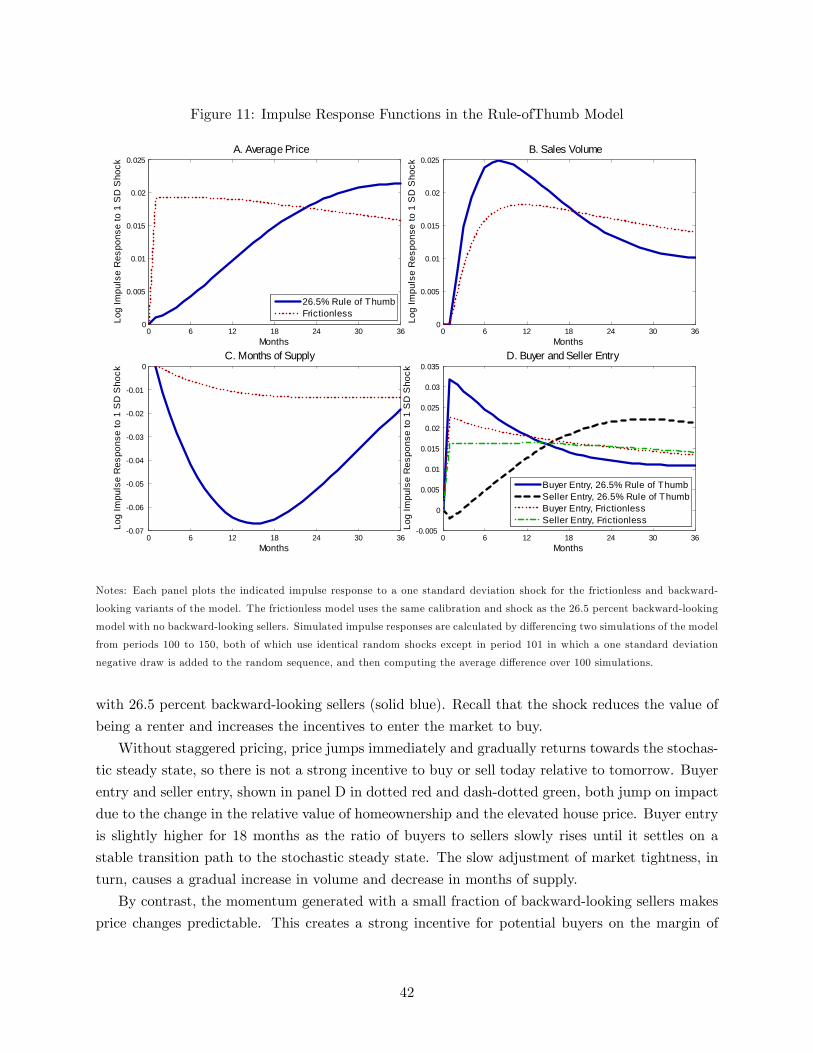
Figure 11: Impulse Response Functions in the Rule-ofThumb Model

0 6 12 18 24 30 360

0.005

0.01

0.015

0.02

0.025

Months

Log 

Impu

lse 

Res

pons

e to

 1 S

D S

hock

A. Average Price

26.5% Rule of ThumbFrictionless

0 6 12 18 24 30 360

0.005

0.01

0.015

0.02

0.025B. Sales Volume

Months

Log 

Impu

lse 

Res

pons

e to

 1 S

D S

hock

0 6 12 18 24 30 36­0.07

­0.06

­0.05

­0.04

­0.03

­0.02

­0.01

0C. Months of Supply

Months

Log 

Impu

lse 

Res

pons

e to

 1 S

D S

hock

0 6 12 18 24 30 36­0.005

0

0.005

0.01

0.015

0.02

0.025

0.03

0.035D. Buyer and Seller Entry

Months

Log 

Impu

lse 

Res

pons

e to

 1 S

D S

hock

Buyer Entry, 26.5% Rule of ThumbSeller Entry, 26.5% Rule of ThumbBuyer Entry, FrictionlessSeller Entry, Frictionless

Notes: Each panel plots the indicated impulse response to a one standard deviation shock for the frictionless and backward-

looking variants of the model. The frictionless model uses the same calibration and shock as the 26.5 percent backward-looking

model with no backward-looking sellers. Simulated impulse responses are calculated by di¤erencing two simulations of the model

from periods 100 to 150, both of which use identical random shocks except in period 101 in which a one standard deviation

negative draw is added to the random sequence, and then computing the average di¤erence over 100 simulations.

with 26.5 percent backward-looking sellers (solid blue). Recall that the shock reduces the value of

being a renter and increases the incentives to enter the market to buy.

Without staggered pricing, price jumps immediately and gradually returns towards the stochas-

tic steady state, so there is not a strong incentive to buy or sell today relative to tomorrow. Buyer

entry and seller entry, shown in panel D in dotted red and dash-dotted green, both jump on impact

due to the change in the relative value of homeownership and the elevated house price. Buyer entry

is slightly higher for 18 months as the ratio of buyers to sellers slowly rises until it settles on a

stable transition path to the stochastic steady state. The slow adjustment of market tightness, in

turn, causes a gradual increase in volume and decrease in months of supply.

By contrast, the momentum generated with a small fraction of backward-looking sellers makes

price changes predictable. This creates a strong incentive for potential buyers on the margin of

42

entering to enter today and for sellers on the margin of entering to wait to do so until prices rise.51

The entry responses are visible in panel D as a gap opens up between the solid blue line,

which represents buyer entry with 26.5 percent backward-looking sellers, and the dotted red line,

which corresponds to buyer entry in a frictionless model. A similar gap opens up for sellers,

as shown by the dashed black line (26.5 percent backward-looking) and the dash-dotted green

line (frictionless). Volume picks up and the growth in sales, overshooting of buyer entry, and

undershooting of seller entry relative to the frictionless case together cause inventory to adjust

more rapidly and substantially than it does in the frictionless model, as shown in panel C. The

stock of renters becomes depleted and the stock of homeowners becomes enlarged to the extent

that 15 months after the shock, they reverse roles and overshoot the frictionless price path again.

This causes inventory and sales volume to mean revert more quickly. In fact, inventory and sales

overshoot the frictionless impulse response once again as prices begin to stabilize due to the glut of

sellers and lack of buyers. These responses look similar to the panel VAR presented in Section 2.

6.2 Explaining the Housing Cycle Facts

6.2.1 Buyer and Seller Entry

Forward looking entry responses imply that seller entry and buyer entry move in opposite directions

at peaks and troughs, corresponding to periods of sudden inventory adjustment, as shown for the

recent boom and bust in Figure 2. While the impulse responses illustrate a similar pattern in

the model, Figure 12 provides further con�rmation of the model�s ability to replicate the data by

showing a sample simulation that looks strikingly similar to Figure 2. Initially there is a sellers�

market in which inventory is low, and buyer and seller entry track one another. When the market

peaks, buyer entry dries up but seller entry remains high as sellers seek to sell to buyers who need

to buy now and are willing to pay high prices. As a result, inventory quickly spikes. When buyers

�nally re-enter the market, seller entry lags and the inventory glut dissipates.

6.2.2 The Relative Volatility of Price, Volume and Inventory

In housing search models without momentum, inventory and volume are too smooth relative to

the data. The top half of Table 8 shows the standard deviation of annual changes of log price, log

volume, and log months of supply in the data and three versions of the model. In the frictionless

price model, months of supply is about a �fth as volatile and volume less than half as volatile as

the data.

This is not unique to my particular frictionless model. In a broad class of housing search models,

combining the steady-state value of being a seller with the steady-state price and di¤erentiating

51 In the model, this operates through the entry cuto¤s c�t and k�t , which are de�ned by di¤erences of value functions

in equations (9) and (10). For instance, the cuto¤ cost for a renter to enter k�t = V rt �V b

t . Because the value functionof being a renter V r

t accounts for the likelihood of getting a shock and entering as a buyer in the future, whenprices are expected to rise V r

t falls relative to Vbt , k

�t falls, and the mass of buyer entrants, which is proportional to

1�K (k�t ), rises.

43

Figure 12: Sample Simulation of Entry, Volume, and Homes For Sale

0 1 2 3 4 5 6 7 8 9 100.008

0.01

0.012

0.014

Mas

s of

 Ent

rant

s in

 Qua

rter

Years0 1 2 3 4 5 6 7 8 9 10

0.02

0.04

0.06

0.08

Mas

s of

 Hom

es fo

r Sal

e

Buyer EntrySalesSeller EntryHomes for Sale

Notes: This �gure shows buyer entry, seller entry, sales, and the stock of homes listed for sale from a simulation of the

backward-looking variant of the model with 26.5 percent backward-looking sellers.

yields:dp

dPr [Sell]=Seller Surplus

1� � .

This steady state response illustrates that if the seller surplus is not miniscule, price is very sensitive

to the probability of sale, which is mechanically related to inventory and volume.52 The relative

volatility of volume and inventory are also low due to the gradual dynamic adjustment of market

tightness as shown in the impulse responses.

The low volatility of inventory is directly analogous to labor search models. Shimer (2005)

shows that unless the employer surplus is tiny, labor search models have di¢ culty accounting for

the volatility of unemployment because most of the response to a shock is absorbed by the wage.

Here, the unemployment rate is analogous to inventory and the wage rate is analogous to price.

Like sticky wages in labor search models, momentum makes house prices adjust more slowly and

slightly reduces price volatility. Quantities adjust slightly more and inventory adjusts substantially

more, as shown in the impulse responses and Table 8, which shows the standard deviation of annual

changes for log price, log sales, and log inventory averaged over 200 500-year simulations. Inventory

is somewhat too volatile in the calibrated model, although it is of the same order of magnitude as

52Diaz and Jerez (2013) explain the relative volatilities in a model without momentum by using a calibration inwhich the seller surplus is 0.5% of the purchase price. Consequently, they argue that price is too insensitive andvolume and time on the market are too sensitive to shocks and introduce a model with ampli�ed price volatility. Mycalibration, which uses a seller surplus that is approximately 7.5% of the steady state price, implies that price is toovolatile in a frictionless setting. Head et al. (2014) make a similar point that momentum reduces price volatility.

44

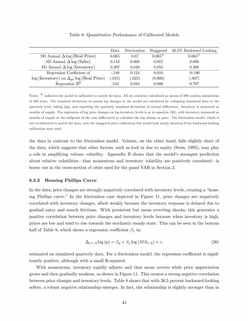
Table 8: Quantitative Performance of Calibrated Models

Data Frictionless Staggered 26.5% Backward LookingSD Annual � log (Real Price) 0.065 0.67 0.065} 0.065}

SD Annual � log (Sales) 0.143 0.060 0.057 0.090SD Annual � log (Inventory) 0.207 0.040 0.055 0.306Regression Coe¢ cient of -.140 0.124 0.010 -0.196

log (Inventory) on �yr log (Real Price) (.015) (.023) (0.006) (.007)Regression R2 .543 0.034 0.000 0.797

Notes: } indicates the model is calibrated to match the data. All are statistics calculated as means of 200 random simulations

of 500 years. The standard deviations of annual log changes in the model are calculated by collapsing simulated data to the

quarterly level, taking logs, and reporting the quarterly standard deviations of annual di¤erences. Inventory is measured as

months of supply. The regression of log price changes on log inventory levels is as in equation (26), with inventory measured as

months of supply at the midpoint of the year di¤erenced to calculate the log change in price. The frictionless model, which is

not recalibrated to match the data, uses the staggered price calibration but would look nearly identical if the backward-looking

calibration were used.

the data in contrast to the frictionless model. Volume, on the other hand, falls slightly short of

the data, which suggests that other factors, such as lock in due to equity (Stein, 1995), may play

a role in amplifying volume volatility. Appendix B shows that the model�s strongest prediction

about relative volatilities� that momentum and inventory volatility are positively correlated� is

borne out in the cross-section of cities used for the panel VAR in Section 2.

6.2.3 Housing Phillips Curve

In the data, price changes are strongly negatively correlated with inventory levels, creating a �hous-

ing Phillips curve.� In the frictionless case depicted in Figure 11, price changes are negatively

correlated with inventory changes, albeit weakly because the inventory response is delayed due to

gradual entry and search frictions. With persistent but mean reverting shocks, this generates a

positive correlation between price changes and inventory levels because when inventory is high,

prices are low and tend to rise towards the stochastic steady state. This can be seen in the bottom

half of Table 8, which shows a regression coe¢ cient �1 in:

�t;t�4 log (p) = �0 + �1 log (MSt�2) + ", (26)

estimated on simulated quarterly data. For a frictionless model, the regression coe¢ cient is signif-

icantly positive, although with a small R-squared.

With momentum, inventory rapidly adjusts and then mean reverts while price appreciation

grows and then gradually weakens, as shown in Figure 11. This creates a strong negative correlation

between price changes and inventory levels. Table 8 shows that with 26.5 percent backward-looking

sellers, a robust negative relationship emerges. In fact, the relationship is slightly stronger than in

45

the data with an R-squared of nearly 0.8. Appendix B shows that the housing Phillips curve is

stronger, both in terms of the magnitude of �1 and in terms of explanatory power, in cities with

more momentum. This is consistent with the model.

7 Conclusion

The degree and persistence of autocorrelation in house price changes is one of the housing market�s

most distinctive features and greatest puzzles. This paper introduces a mechanism that ampli�es

small frictions that have been discussed in the literature into substantial momentum. Search

frictions and concave demand in relative price together imply that increasing one�s list price above

the market average is costly, while lowering one�s list price below the market average has little

bene�t. This strategic complementarity induces sellers to set their list prices close to the market

average. Consequently, modest initial price insensitivity to changes in fundamentals can lead to

prolonged periods of autocorrelated price changes as sellers slowly adjust their list price to remain

close to the mean.

This ampli�cation mechanism depends critically on a concave e¤ect of unilaterally changing a

house�s list price relative to the average on the probability of sale. I identify this e¤ect in micro data

by instrumenting for list price with a proxy for the equity position of sellers and �nd statistically

and economically signi�cant concavity.

To demonstrate the strategic complementarity�s ability to prolong an initial source of price

insensitivity, I introduce an equilibrium search model in which buyers avoid looking at homes they

perceive to be overpriced. I calibrate the model to the micro data and consider the quantitative

impact of two di¤erent sources of insensitivity. A two-month staggered pricing friction is ampli�ed

into ten months of autocorrelated price changes. If just 26.5 percent of sellers use a backward-

looking rule of thumb, the impulse response to a shock lasts for three years, as in the data. Without

concave demand, 78 to 93 percent of sellers would have to be backward-looking. The ampli�cation

channel also interacts with other frictions that have been discussed by the literature. In particular,

concave demand in relative price would substantially amplify momentum created by learning in

an �islands�model because learning about higher order beliefs is particularly sluggish. Assessing

whether such a model can explain the momentum in the data without a small number of non-

rational sellers is a promising path for future research.

Momentum has a substantial impact on housing dynamics because it causes forward-looking

buyers and sellers to re-time their entry into the housing market in order to sell high and buy low.

These buyer and seller entry patterns can help explain the relative volatilities of price, volume, and

inventory, the �housing Phillips curve�relationship between price changes and inventory levels, and

the sudden reversals between buyers�and sellers�markets that occurs at peaks and troughs.

Beyond the housing market, this paper shows how a central idea in macroeconomics� that

strategic complementarities can greatly amplify modest frictions� can be applied in new contexts.

These contexts can, in turn, serve as empirical laboratories to study macroeconomic phenomena

46

for which micro evidence has proven elusive. In particular, many models with real rigidities (Ball

and Romer, 1990) use a concave demand curve. This paper provides new evidence that a concave

demand curve in relative price is not merely a theoretical construct and can have a signi�cant e¤ect

on market dynamics.

47

References

Abraham, J. M. and P. H. Hendershott (1996). Bubbles in Metropolitan Housing Markets. Jour-nal of Housing Research 7 (2), 191�207.

Adjemian, S., H. Bastani, M. Juillard, K. Frederic, F. Mihoubi, G. Perendia, J. Pfeifer, M. Ratto,and S. Villemot (2011). Dynare: Reference Manual, Version 4.

Albrecht, J., P. A. Gautier, and S. Vroman (2013). Directed Search in the Housing Market.

Anenberg, E. (2013). Information Frictions and Housing Market Dynamics.

Anenberg, E. and P. Bayer (2013). Endogenous Sources of Volatility in Housing Markets: TheJoint Buyer-Seller Problem.

Angeletos, G.-M. and J. La�O (2013). Sentiments. Econometrica 81 (2), 739�779.

Anglin, P. M., R. Rutherford, and T. Springer (2003). The Trade-o¤ Between the Selling Priceof Residential Properties and Time-on-the-Market: The Impact of Price Setting. Journal ofReal Estate Finance and Economics 26 (1), 95�111.

Arellano, M. and O. Bover (1995). Another Look at the Instrumental Variable Estimation ofError-Components Models. Journal of Econometrics 68, 29�51.

Ball, L. and D. Romer (1990). Real Rigidities and the Non-Neutrality of Money. The Review ofEconomic Studies 57 (2), 183�203.

Barberis, N., A. Shleifer, and R. Vishny (1998). A Model of Investor Sentiment. Journal ofFinancial Economics 49, 307�343.

Barsky, R., C. L. House, and M. Kimball (2007). Sticky-Price Models and Durable Goods.American Economic Review 97 (3), 984�998.

Benabou, R. (1992). In�ation and E¢ ciency in Search Markets. The Review of Economic Stud-ies 59 (2), 299�329.

Berkovec, J. A. and J. L. Goodman (1996). Turnover as a Measure of Demand for ExistingHomes. Real Estate Economics 24 (4), 421�440.

Bils, M., P. J. Klenow, and B. A. Malin (2012). Reset Price In�ation and the Impact of MonetaryPolicy Shocks. American Economic Review 102 (6), 2798�2825.

Burnside, C., S. Rebelo, and M. Eichenbaum (2013). Understanding Booms and Busts in HousingMarkets.

Calvo, G. (1983). Staggered Prices in a Utility-Maximizing Framework. Journal of MonetaryEconomics 12 (3), 383�398.

Campbell, J. Y. and N. G. Mankiw (1989). Consumption, Income, and Interest Rates: Reinter-preting the Time Series Evidence. In O. J. Blanchard and S. Fischer (Eds.), NBER Macro-economics Annual 1989, Volume 4, pp. 185�246. Cambridge, MA: MIT Press.

Caplin, A. and J. Leahy (2011). Trading Frictions and House Price Dynamics. Journal of Money,Credit and Banking 43 (7), 283�303.

Capozza, D. R., P. H. Hendershott, and C. Mack (2004). An Anatomy of Price Dynamics inIlliquid Markets: Analysis and Evidence from Local. Real Estate Economics 32 (1), 1�32.

Carrillo, P. E. (2012). An Empirical Stationary Equilibrium Search Model of the Housing Market.International Economic Review 53 (1), 203�234.

48

Case, K. E. (2008). The Central Role of Home Prices in the Current Financial Crisis: How Willthe Market Clear? Brookings Papers on Economic Activity (Fall), 161�193.

Case, K. E. and R. J. Shiller (1987). Prices of Single-Family Homes Since 1970: New Indices forFour Cities. New England Economic Review (September), 45�56.

Case, K. E. and R. J. Shiller (1989). The E¢ ciency of the Market for Single-Family Homes.American Economic Reivew 79 (1), 125�137.

Case, K. E., R. J. Shiller, and A. K. Thompson (2012). What Have They Been Thinking?Homebuyer Behavior in Hot and Cold Markets. Brookings Papers on Economic Activity (Fall),265�298.

Chari, V., P. J. Kehoe, and E. R. McGrattan (2000). Sticky Price Models of the Business Cycle:Can the Contract Multiplier Solve the Persistence Problem? Econometrica 68 (5), 1151�1179.

Chen, Y. and R. W. Rosenthal (1996). Asking Prices as Commitment Devices. InternationalEconomic Review 37 (1), 129�155.

Cho, M. (1996). House Price Dynamics: A Survey of Theoretical and Empirical Issues. Journalof Housing Research 7 (2), 145�172.

Coibion, O. and Y. Gorodnichenko (2011). Strategic Interaction Among Heterogeneous Price-Setters in an Estimated DSGE Model. The Review of Economics and Statistics 93 (3), 920�940.

Cooper, R. and A. John (1988). Coordinating Coordination Failures in Keynesian Models. Quar-terly Journal of Economics 103 (3), 441�463.

Cutler, D. M., J. M. Poterba, and L. H. Summers (1991). Speculative Dynamics. Review ofEconomic Studies 58 (3), 529�546.

de Wit, E. R. and B. van der Klaauw (2013). Asymmetric Information and List-Price Reductionsin the Housing Market. Regional Science and Urban Economics 43 (3), 507�520.

Diaz, A. and B. Jerez (2013). House Prices, Sales, and Time on the Market: A Search-TheoreticFramework. International Economic Review 54 (3), 837�872.

Fehr, E. and J.-R. Tyran (2005). Individual Irrationality and Aggregate Outcomes. Journal ofEconomic Perspectives 19 (4), 43�66.

Frazzini, A. (2006). The Disposition E¤ect and Underreaction to News. The Journal of Fi-nance 61 (4), 2017�2046.

Fuhrer, J. C. (2011). In�ation Persistence. In B. Friedman and M. Woodford (Eds.), Handbookof Monetary Economics, Volume 3, Chapter 9, pp. 423�486. Elsevier.

Fuster, A., D. Laibson, and B. Mendel (2010). Natural Expectations and Macroeconomic Fluc-tuations. Journal of Economic Perspectives 24 (4), 67�84.

Gali, J. and M. Gertler (1999). In�ation Dynamics: A Structural Econometric Analysis. Journalof Monetary Economics 44, 195�222.

Genesove, D. and L. Han (2012). Search and Matching in the Housing Market. Journal of UrbanEconomics 72 (1), 31�45.

Genesove, D. and C. Mayer (1997). Equity and Time to Sale in the Real Estate Market. AmericanEconomic Reivew 87 (3), 255�269.

Genesove, D. and C. Mayer (2001). Loss Aversion and Seller Behavior: Evidence From theHousing Market. Quarterly Journal of Economics 116 (4), 1233�1260.

49

Glaeser, E. L., J. Gyourko, E. Morales, and C. G. Nathanson (2013). Housing Dynamics.

Golosov, M. and R. E. Lucas (2008). Menu Costs and Phillips Curves. Journal of PoliticalEconomy 115 (2), 171�199.

Gopinath, G. and O. Itskhoki (2010). In Search of Real Rigidities. In D. Acemoglu and M. Wood-ford (Eds.), NBER Macroeconomics Annual, Volume 25, pp. 261�310. Chicago: University ofChicago Press.

Guren, A. and T. McQuade (2013). How Do Foreclosures Exacerbate Housing Downturns?

Haltiwanger, J. and M. Waldman (1989). Limited Rationality and Strategic Complements: theImplications for Macroeconomics. The Quarterly Journal of Economics 104 (3), 463�483.

Han, L. and W. C. Strange (2012). What is the Role of the Asking Price for a House.

Haurin, D. R. and H. L. Gill (2002). The Impact of Transaction Costs and the Expected Lengthof Stay on Homeownership. Journal of Urban Economics 51, 563�584.

Haurin, D. R., J. L. Haurin, T. Nadauld, and A. Sanders (2010, December). List Prices, SalePrices and Marketing Time: An Application to U.S. Housing Markets. Real Estate Eco-nomics 38 (4), 659�685.

Hausman, J. A., H. Ichimura, W. K. Newey, and J. L. Powell (1991). Identi�cation and Estimationof Polynomial Errors-In-Variables Models. Journal of Econometrics 50 (3), 273�295.

Head, A., H. Lloyd-Ellis, and H. Sun (2014). Search , Liquidity , and the Dynamics of HousePrices and Construction. American Economic Review 104 (4), 1172�1210.

Hong, H. and J. C. Stein (1999). A Uni�ed Theory of Underreaction, Momentum Trading, andOverreaction in Asset Markets. The Journal of Finance 54 (6), 2143�2184.

Kang, H. B. and J. Gardner (1989). Selling Price and Marketing Time in the Residential RealEstate Market. The Journal of Real Estate Research 4 (1), 21�35.

Kim, J., S. Kim, E. Schaumburg, and C. A. Sims (2008). Calculating and Using Second-OrderAccurate Solutions of Discrete Time Dynamic Equilibrium Models. Journal of EconomicDynamics and Control 32 (11), 3397�3414.

Kimball, M. (1995). The Quantitative Analytics of the Basic Neomonetarist Model. Journal ofMoney, Credit and Banking 27 (4), 1241�1277.

Klenow, P. J. and J. L. Willis (2006). Real Rigidities and Nominal Price Changes.

Knight, J. R. (2002). Listing Price, Time on Market, and Ultimate Selling Price: Causes andE¤ects of Listing Price Changes. Real Estate Economics 30 (2), 213�237.

Krainer, J. (2001). A Theory of Liquidity in Residential Real Estate Markets. Journal of UrbanEconomics 49 (1), 32�53.

Kudoh, N. (2013). Price Competition with Search Frictions.

Lazear, E. P. (2010). Why Do Inventories Rise When Demand Falls in Housing and OtherMarkets?

Leamer, E. E. (2007). Housing is the Business Cycle. In Housing, Housing Finance and MonetaryPolicy, A Symposium, pp. 149�233. Federal Reserve of Kansas City.

Lester, B., L. Visschers, and R. Woltho¤ (2013). Competing With Asking Prices.

Levin, A. and T. Yun (2009). Reconsidering the Microeconomic Foundations of Price-SettingBehavior.

50

Levitt, S. D. and C. Syverson (2008). Market Distortions When Agents Are Better Informed:The Value of Information in Real Estate Transactions. The Review of Economics and Statis-tics 90 (4), 599�611.

Lorenzoni, G. (2009). A Theory of Demand Shocks. American Economic Review 99 (5), 2050�2084.

Lucas, R. E. (1972). Expectations and the Neutrality of Money. Journal of Economic Theory 4,103�124.

Malpezzi, S. (1999). A Simple Error Correction Model of House Prices. Journal of HousingEconomics 8 (1), 27�62.

Meen, G. (2002). The Time-Series Behavior of House Prices: A Transatlantic Divide? Journalof Housing Economics 11 (1), 1�23.

Meese, R. A. and N. Wallace (1997). The Construction of Residential Housing Price Indices: AComparison of Repeat-Sales, Hedonic-Regression, and Hybrid Approaches. Journal of RealEstate Finance and Economics 14, 51�73.

Moskowitz, T. J., Y. H. Ooi, and L. H. Pedersen (2012, May). Time Series Momentum. Journalof Financial Economics 104 (2), 228�250.

Murphy, K. M. and R. H. Topel (1985). Estimation and Inference in Two-Step EconometricModels. Journal of Business and Economic Statistics 3 (4), 370�379.

Nakamura, E. and D. Zerom (2010). Accounting for Incomplete Pass-Through. Review of Eco-nomic Studies 77, 1192�1230.

Ngai, L. R. and S. Tenreyro (2013). Hot and Cold Seasons in the Housing Market.

Novy-Marx, R. (2009). Hot and Cold Markets. Real Estate Economics 37 (1), 1�22.

Ortalo-Magné, F. and S. Rady (2006). Housing Market Dynamics: On the Contribution of IncomeShocks and Credit Constraints. Review of Economic Studies 73, 459�485.

Peach, R. (1983). An Econometric Model of Investment in Single Family Homes. Ph. D. thesis,University of Maryland.

Phelps, E. S. (1983). The Trouble With �Rational Expectations�and the Problem of In�ationStabilization. In R. Frydman and E. S. Phelps (Eds.), Individual Forecasting and AggregateOutcomes. Cambridge University Press.

Piazzesi, M. and M. Schneider (2009). Momentum Traders in the Housing Market: Survey Evi-dence and a Search Model. American Economic Review 99 (2), 406�411.

Poterba, J. and T. Sinai (2008). Tax Expenditures for Owner-Occupied Housing: Deductionsfor Property Taxes and Mortgage Interest and the Exclusion of Imputed Rental Income.American Economic Review 98 (2), 84�89.

Shimer, R. (2005). The Cyclical Behavior of Equilibrium Unemployment and Vacancies. Ameri-can Economic Review 95 (1), 25�49.

Smets, F. and R. Wouters (2007). Shocks and Frictions in U.S. Business Cycles: A BayesianDSGE Approach. American Economic Review 97 (3), 586�606.

Stein, J. C. (1995). Prices and Trading Volume in the Housing Market: A Model with Down-Payment E¤ects. Quarterly Journal of Economics 110 (2), 379�406.

Stiglitz, J. (1979). Equilibrium in Product Markets with Imperfect Information. American Eco-nomic Review 69 (2), 339�345.

51

Taylor, C. R. (1999, July). Time-on-the-Market as a Sign of Quality. Review of Economic Stud-ies 66 (3), 555�578.

Taylor, J. B. (1980). Aggregate Dynamics and Staggered Contracts. Journal of Political Econ-omy 88 (1), 1�23.

Wheaton, W. C. (1990). Vacancy, Search, and Prices in a Housing Market Matching Model.Journal of Political Economy 98 (6), 1270�1292.

Wheaton, W. C. and N. J. Lee (2009). The Co-Movement of Housing Sales and Housing Prices:Empirics and Theory.

Woglom, G. (1982). Underemployment Equilibrium With Rational Expectations. The QuarterlyJournal of Economics 97 (1), 89�107.

Woodford, M. (2003). Imperfect Common Knowledge and the E¤ects of Monetary Policy. InP. Aghion, R. Frydman, J. Stiglitz, and M. Woodford (Eds.), Knowledge, Information, andExpectations in Modern Macroeconomics: In Honor of Edmund S. Phelps. Princeton Univer-sity Press.

Yavas, A. and S. Yang (1995). The Strategic Role of Listing Price in Marketing Real Estate:Theory and Evidence. Real Estate Economics 23 (3), 347�368.

52

A Data

A.1 Time Series Data

A.1.1 National and Regional Data

In the main text, three data series are used for price, volume and inventory:

� The CoreLogic national repeat-sales house price index. This is an arithmetic interval-weightedhouse price index from January 1976 to August 2013. The monthly index is averaged at aquarterly frequency and adjusted for in�ation using the Consumer Price Index, BLS seriesCUUR0000SA0.

� The National Association of Realtors� series of sales of existing single-family homes at aseasonally-adjusted annual rate. The data is monthly for the whole nation from January1968 to January 2013 and available on request from the NAR. The monthly data is averagedat a quarterly frequency.

� Homes listed for sale comes from vacant homes listed for sale from the Census HousingVacancy Survey, quarterly from Q1 1968 to Q4 2012. This is divided by the NAR salesvolume series to create months of supply.

Other price and inventory measures are used in Appendix B. The price measures include:

� A median sales price index for existing single-family homes. The data is monthly for thewhole nation from January 1968 to January 2013 and available on request from the NationalAssociation of Realtors.

� The quarterly national �expanded purchase-only� HPIs that only includes purchases andsupplements the FHFA�s database from the GSEs with deeds data from DataQuick from Q11991 to Q4 2012. This is an interval-weighted geometric repeat-sales index.

� The monthly Case-Shiller Composite Ten from January 1987 to January 2013. This is aninterval-weighted arithmetic repeat-sales index.

� Amedian sales price index for all sales (existing and new homes) from CoreLogic from January1976 to August 2013.

The additional inventory measure is the National Association of Realtors�series on inventoryand months of supply of existing single-family homes. The data is monthly for the whole nationfrom June 1982 to February 2013 and is available on request.

For annual AR(1) regressions, I use non-seasonally-adjusted data. Because the volume seriescomes seasonally adjusted, for any analysis that includes sales volume, I use the data provider�sseasonal adjustment if available and otherwise seasonally adjust the data using the Census Bureau�sX-12 ARIMA software using a multiplicative seasonal factor.

A.1.2 City-Level Data

I create two city-level data sets. The �rst consists of local repeat-sales price indices for 103 CBSAdivisions from CoreLogic. These CBSAs divisions include all CBSAs divisions that are part of the100 largest CBSAs which have data from at least 1995 onwards. Most of these CBSAs have data

53

Table 9: CBSAs in CoreLogic City-Level Price Data Set

CBSA Code Main City Name Start End 32820 Memphis, TN 1984 2013

10420 Akron, OH 1978 2013 33124 Miami, FL 1976 2013

10580 Albany, NY 1992 2013 33340 Milwaukee, WI 1976 2013

10740 Albuquerque, NM 1992 2013 33460 Minneapolis, MN 1976 2013

10900 Allentown, PA 1976 2013 34980 Nashville, TN 1976 2013

12060 Atlanta, GA 1976 2013 35004 Nassau, NY 1976 2013

12420 Austin, TX 1976 2013 35084 Newark, NJ-PA 1976 2013

12540 Bakers�eld, CA 1976 2013 35300 New Haven, CT 1985 2013

12580 Baltimore, MD 1976 2013 35380 New Orleans, LA 1976 2013

12940 Baton Rouge, LA 1992 2013 35644 New York, NY 1976 2013

13140 Beaumont, TX 1993 2013 36084 Oakland, CA 1976 2013

13644 Bethesda, MD 1976 2013 36420 Oklahoma City, OK 1976 2013

13820 Birmingham, AL 1976 2013 36540 Omaha, NE 1990 2013

14484 Boston, MA 1976 2013 36740 Orlando, FL 1976 2013

14860 Bridgeport, CT 1976 2013 37100 Ventura, CA 1976 2013

15380 Bu¤alo, NY 1991 2013 37764 Peabody, MA 1976 2013

15764 Cambridge, MA 1976 2013 37964 Philadelphia, PA 1976 2013

15804 Camden, NJ 1976 2013 38060 Phoenix, AZ 1976 2013

16700 Charleston, SC 1976 2013 38300 Pittsburgh, PA 1976 2013

16740 Charlotte, NC 1976 2013 38900 Portland, OR 1976 2013

16974 Chicago, IL 1976 2013 39100 Poughkeepsie, NY 1976 2013

17140 Cincinnati, OH 1976 2013 39300 Providence, RI 1976 2013

17460 Cleveland, OH 1976 2013 39580 Raleigh, NC 1976 2013

17820 Colorado Springs, CO 1976 2013 40060 Richmond, VA 1976 2013

17900 Columbia, SC 1977 2013 40140 Riverside, CA 1976 2013

18140 Columbus, OH 1976 2013 40380 Rochester, NY 1991 2013

19124 Dallas, TX 1977 2013 40484 Rockingham County, NH 1990 2013

19380 Dayton, OH 1976 2013 40900 Sacramento, CA 1976 2013

19740 Denver, CO 1976 2013 41180 St. Louis, MO 1978 2013

19804 Detroit, MI 1989 2013 41620 Salt Lake City, UT 1992 2013

20764 Edison, NJ 1976 2013 41700 San Antonio, TX 1991 2013

21340 El Paso, TX 1977 2013 41740 San Diego, CA 1976 2013

22744 Fort Lauderdale, FL 1976 2013 41884 San Francisco, CA 1976 2013

23104 Fort Worth, TX 1984 2013 41940 San Jose, CA 1976 2013

23420 Fresno, CA 1976 2013 42044 Santa Ana, CA 1976 2013

23844 Gary, IN 1992 2013 42644 Seattle, WA 1976 2013

24340 Grand Rapids, MI 1992 2013 44140 Spring�eld, MA 1976 2013

24660 Greensboro, NC 1976 2013 44700 Stockton, CA 1976 2013

24860 Greenville, SC 1976 2013 45060 Syracuse, NY 1992 2013

25540 Hartford, CT 1976 2013 45104 Tacoma, WA 1977 2013

26180 Honolulu, HI 1976 2013 45300 Tampa, FL 1976 2013

26420 Houston, TX 1982 2013 45780 Toledo, OH 1976 2013

26900 Indianapolis, IN 1991 2013 45820 Topeka, KS 1985 2013

27260 Jacksonville, FL 1976 2013 46060 Tucson, AZ 1976 2013

28140 Kansas City, MO 1985 2013 46140 Tulsa, OK 1981 2013

28940 Knoxville, TN 1977 2013 47260 Virginia Beach, VA 1976 2013

29404 Lake County, IL 1982 2013 47644 Warren, MI 1976 2013

29820 Las Vegas, NV 1983 2013 47894 Washington, DC 1976 2013

30780 Little Rock, AR 1985 2013 48424 West Palm Beach, FL 1976 2013

31084 Los Angeles, CA 1976 2013 48620 Wichita, KS 1986 2013

31140 Louisville, KY 1987 2013 48864 Wilmington, DE 1976 2013

32580 McAllen, TX 1992 2013 49340 Worcester, MA 1976 2013

54

Table 10: MSAs in Merged Price-Inventory-Volume Panel

Principal City First Date Last Date Obs Principal City First Date Last Date Obs

Akron, OH 1990, Q1 2013, Q1 87 Miami, FL 1993, Q1 2013, Q1 69

Allentown, PA 1999, Q1 2013, Q1 50 Milwaukee, WI 1998, Q1 2013, Q1 61

Atlanta, GA 1999, Q1 2012, Q3 55 Nashville, TN 1999, Q3 2013, Q1 55

Austin, TX 1994, Q1 2013, Q1 66 New Brunswick, NJ 1999, Q1 2013, Q1 57

Baltimore, MD 1999, Q1 2013, Q1 57 New York, NY 1999, Q1 2013, Q1 57

Charleston, SC 1997, Q1 2013, Q1 65 Newark, NJ 1998, Q1 2013, Q1 61

Chicago, IL 1999, Q1 2013, Q1 57 Oklahoma City, OK 1990, Q1 2013, Q1 79

Cincinnati, OH 1990, Q1 2006, Q4 51 Omaha, NE-IA 2000, Q3 2013, Q1 51

Columbia, SC 1995, Q1 2013, Q1 61 Phoenix, AZ 1993, Q2 2012, Q2 74

Columbus, OH 1995, Q2 2013, Q1 69 Portland, OR 1994, Q1 2011, Q3 66

Dallas, TX 2000, Q1 2013, Q1 53 Providence, RI 1994, Q1 2013, Q1 71

Denver, CO 1999, Q1 2013, Q1 57 Raleigh, NC 1991, Q2 2008, Q2 55

Greenville, SC 1994, Q1 2013, Q1 60 Richmond, VA 1990, Q1 2009, Q2 57

Honolulu, HI 1999, Q1 2013, Q1 57 San Antonio, TX 1998, Q2 2013, Q1 60

Houston, TX 1999, Q3 2013, Q1 55 San Diego CA 1997, Q1 2013, Q1 65

Kansas City, MO 1998, Q3 2012, Q3 57 San Francisco, CA 1992, Q2 2009, Q4 58

Knoxville, TN 1998, Q1 2013, Q1 57 Santa Ana, CA 1999, Q1 2013, Q1 57

Las Vegas, NV 1992, Q2 2013, Q1 63 St. Louis, MO 1996, Q2 2013, Q1 64

Little Rock, AR 1998, Q3 2013, Q1 59 Tampa, FL 1999, Q1 2013, Q1 57

Los Angeles, CA 1993, Q3 2013, Q1 79 Tulsa, OK 1999, Q1 2013, Q1 57

Memphis, TN 1994, Q2 2013, Q1 76 Washington, DC 1993, Q2 2013, Q1 72

starting in 1976. See Table 9 for the full list of CBSAs and years. This data is used for the annualAR(1) regression coe¢ cient histogram in Figure 1 and is adjusted for in�ation using the CPI.

The second city-level data set is used for the panel VAR and several cross-city comparisonsin Appendix B. It combines the same CoreLogic city-level repeat-sales house price indices withtransaction volume data for existing home sales from CoreLogic and months of supply at the MSAlevel provided by the National Association of Realtors. The CoreLogic and NAR data sets aremerged using the principal city of the MSA and CBSA division. The volume series sometimes havediscontinuities corresponding to the introduction of an additional county to a CBSA, so I examineeach time series and select a starting date for the volume series for each CBSA division equal to themonth after the last discontinuity. Similarly, the NAR months of supply measure is occasionally notreported for a given MSA. I drop all prior quarters if there are four continuous quarters of missingdata. There are, however, a few interspersed quarters with missing data. The similarity betweenthe panel VAR and a VAR on national data shows that the missing quarters are not driving theresults. Each MSA�s start quarter and end quarter are the �rst and last quarters, respectively,for which both volume and inventory data are available, with the inventory data typically beingthe binding constraint. Finally, I limit the sample to 42 MSAs with at least 50 quarters of bothinventory and volume data. Table 10 summarizes the full list of MSAs and years in the data set.

A.2 Micro Data

The matched listings-transactions micro data covers the San Francisco Bay, San Diego, and LosAngeles metropolitan areas. The San Francisco Bay sample includes Alameda, Contra Costa,Marin, San Benito, San Francisco, San Mateo, and Santa Clara counties. The Los Angeles sampleincludes Los Angeles and Orange counties. The San Diego sample only includes San Diego County.

55

The data from DataQuick run from January 1988 to August 2013. The Altos data run from October2007 to May 2013. I limit my analysis to April 2008 to February 2013, as described in footnote 14.

A.2.1 DataQuick Characteristic and History Data Construction

The DataQuick data is provided in separate assessor and history �les. The assessor �le containshouse characteristics from the property assessment and a unique property ID for every parcel ina county. The history �le contains records of all deed transfers, with each transfer matched to aproperty ID. Several steps are used to clean the data.

First, both data �les are formatted and sorted into county level data �les. For a very smallnumber of properties, data with a typo is replaced as missing.

Second, some transactions appear to be duplicates. Duplicate values are categorized and com-bined into one observation if possible. I drop cases where there are more than ten duplicates, as thisis usually a developer selling o¤ many lots individually after splitting them. Otherwise, I pick thesale with the highest price, or, if as a tiebreaker, the highest loan value at origination. In practice,this a¤ects very few observations.

Third, problematic observations are identi�ed. In particular, transfers between family mem-bers are identi�ed and dropped based on a DataQuick transfer �ag and a comparison buyer andseller names. Sales with prices that are less than or equal to one dollar are also counted as trans-fers. Partial consideration sales, partial sales, group sales, and splits are also dropped, as aredeed transfers that are part of the foreclosure process but not actually transactions. Transactionsthat appear to be corrections or with implausible origination loan to value ratios are also �aggedand dropped. Properties with implausible characteristics (<10 square feet, < 1 bedroom, < 1/2bathroom, implausible year built) have the implausible characteristic replaced as a missing value.

From the �nal data set, I only use resale transactions (as opposed to new construction orsubdivisions) of single-family homes, both of which are categorized by DataQuick.

A.2.2 Altos Research Listings Data Construction and Match to DataQuick

The Altos research data contains address, MLS identi�er, house characteristics, list price, and datefor every week-listing. Altos generously provided me access to an address hash that was used toparse the address �elds in the DataQuick assessor data and Altos data and to create a matchinghash for each. Hashes were only used that appeared in both data �les, and hashes that matchedto multiple DataQuick properties were dropped.

After formatting the Altos data, I match the Altos data to the DataQuick property IDs. I�rst use the address hash, applying the matched property ID to every listing with the same MLSidenti�er (all listings with the same MLS ID are the same property, and if they do not all matchit is because some weeks the property has the address listed di¤erently, for instance �street� isincluded in some weeks but not others). Second, I match listings not matched by the address hashby repeatedly matching on various combinations of address �elds and discarding possible matcheswhen there is not a unique property in the DataQuick data for a particular combination of �elds,which prevents cases where there are two properties that would match from being counted as amatch. I determined the combinations of address �elds on which to match based on an inspectionof the unmatched observations, most of which occur when the listing in the MLS data does notinclude the exact wording of the DataQuick record (e.g., missing �street�). The �elds typicallyinclude ZIP, street name, and street number and di¤erent combinations of unit number, streetdirection, and street su¢ x. In some cases I match to the �rst few digits of street number or the�rst word of a street name. I �nally assign any unmatched observations with the same MLS ID as

56

a matched observation or the same address hash, square feet, year built, ZIP code, and city as amatched observation the property ID of the matched observation. I subsequently work only withmatched properties so that I do not inadvertently count a bad match as a withdrawal.

The observations that are not matched to a DataQuick property ID are usually multi-familyhomes (which I subsequently drop), townhouses with multiple single-family homes at the sameaddress, or listings with typos in the address �eld.

I use the subset of listings matched to a property ID and combine cases where the same propertyhas multiple MLS identi�ers into a contiguous listing to account for de-listings and re-listings ofproperties, which is a common tactic among real estate agents. In particular, I count a listing ascontiguous if the property is re-listed within 13 weeks and there is not a foreclosure between thede-listing and re-listing. I assign each contiguous listing a single identi�er, which I use to match totransactions.

In a few cases, a listing matches to several property IDs. I choose the property ID that matchesto a transaction or that corresponds to the longest listing period. All results are robust to droppingthe small number of properties that match to multiple property IDs.

I �nally match all consolidated listings to a transaction. I drop transactions and correspondinglistings where there was a previous transaction in the last 90 days, as these tend to be a truetransaction followed by several subsequent transfers for legal reasons (e.g., one spouse buys thehouse and then sells half of it to the other). I �rst match to a transaction where the date of lastlisting is in the month of the deed transfer request or in the prior three months. I then matchunmatched listings to a transaction where the date of last listing is in the three months afterthe deed transfer request (if the property was left on the MLS after the request, presumably byaccident). I then repeat the process for unmatched listings for four to 12 months prior and four to12 months subsequent. Most matches have listings within three months of the last listing.

For matched transactions, I generate two measures of whether a house sold within a given timeframe. The �rst, used in the main text, is the time between the date of �rst listing and the dateof �ling of the deed transfer request. The second, used in robustness checks in Appendix C, is thetime between date of �rst listing and the �rst of the last listing date or the transfer request.

Figure 13 shows the fraction of all single-family transactions of existing homes for which mydata accounts in each of the three metropolitan areas over time. Because the match rates start lowin October 2007, I do not start my analysis until April 2008, except in San Diego where almost alllistings have no listed address until August 2008. Besides that, the match rates are fairly stable,except for a small dip in San Diego in mid-2009 and early 2012 and a large fall o¤ in the SanFrancisco Bay area after June 2012. I consequently end the analysis for the San Francisco Bay areaat June 2012. Figures 14, 15, and 16 show match rates by ZIP code. One can see that the matchrate is consistently high in the core of each metropolitan area and falls o¤ in the outlying areas,such as western San Diego county and Escondido in San Diego, Santa Clarita in Los Angeles, andBrentwood and Pleasanton in the San Francisco Bay area.

A.2.3 Construction of House Price Indices

I construct house price indices largely following Case and Shiller (1989) and follow sample restric-tions imposed in the construction of the Case-Shiller and Federal Housing Finance Administration(FHFA) house price indices.

For the repeat sale indices, I drop all non-repeat sales, all sales pairs with less than six monthsbetween sales, and all sales pairs where a �rst stage regression on year dummies shows a propertyhas appreciated by 100 percent more or 100 percent less than the average house in the MSA. I

57

Figure 13: Match Rates by Month of Transaction

0.2

.4.6

.81

Frac

tion 

of T

rans

actio

ns M

atch

ed to

 Lis

ting

2008m1 2009m1 2010m1 2011m1 2012m1 2013m1Date

Bay Area LA SD

Figure 14: Match Rates by ZIP Code: Bay Area

58

Figure 15: Match Rates by ZIP Code: Los Angeles

Figure 16: Match Rates by ZIP Code: San Diego

59

estimate an interval-corrected geometric repeat-sales index at the ZIP code level. This involvesestimating a �rst stage regression:

ph`t = �h` + �t + "h`t, (27)

where p is the log price of a house h in location ` at time t, �h` is a sales pair �xed e¤ect, �t is atime �xed e¤ect, and "h`t is an error term.

I follow Case and Shiller (1989) by using a GLS interval-weighted estimator to account for thefact that longer time intervals tend to have a larger variance in the error of (27). This is typicallyimplemented by regressing the square of the error term "2h`t on a linear (Case-Shiller index) orquadratic (FHFA) function of the time interval between the two sales. The regression coe¢ cientsare then used to construct weights corresponding to 1p

"̂2h`twhere "̂2h`t is a predicted value from the

interval regression. I �nd that the variance of the error of (27) is non-monotonic: it is very high forsales that occur quickly, falls to its lowest level for sales that occur approximately three years afterthe �rst sale, and then rises slowly over time. This is likely due to �ippers who upgrade a houseand sell it without the upgrade showing up in the data. Consequently, I follow a non-parametricapproach by binning the data into deciles of the time interval between the two sales, calculate theaverage "2h`t for the decile �"

2h`t, and weight by

1p�"2h`t. The results are nearly identical using a linear

interval weighting.exp (�t) is then a geometric house price index. The resulting indices can be quite noisy. Conse-

quently, I smooth the index using a 3-month moving average, which produced the lowest predictionerror of several di¤erent window widths. The resulting indices at the MSA level are very comparableto published indices by Case-Shiller, the FHFA, and CoreLogic.

The log predicted value of a house at time t, p̂t, that sold originally at time � for P� is:

p̂t = log

0@ exp��̂t

�exp

��̂�

�P�1A .

For the hedonic house price indices, I use all sales and estimate:

pi`t = �t + �Xi + "i`t; (28)

where Xi is a vector of third-order polynomials in four housing characteristics: age, bathrooms,bedrooms, and log (square feet), all of which are winsorized at the one percent level by countyfor all properties in a county, not just those that trade. Recall that these characteristics are allrecorded as a single snapshot in 2013, so Xi is not time dependent. I do not include a characteristicif over 25 percent of the houses in a given geography are missing data for a particular characteristic.Again exp (�t) is a house price index, which I smooth using a 3-month moving average. The logpredicted price of a house is

p̂it = �̂Xi + �̂i:

For homes that are missing characteristics included in an area�s house price index calculation, Ireplace the characteristic with its average value in a given ZIP code.

For robustness I calculate both indices for the full sample and a non-distressed sample, wherea repeat-sales pair counts as distressed if either sale is an REO sale, a foreclosure auction sale, or ashort sale. For my analysis, I use a ZIP code level index, but all results are robust to alternativelyusing a house price index for all homes within one mile of the centroid of a home�s seven-digit ZIPcode (roughly a few square blocks). I do not calculate a house price index if the area has fewer than

60

Table 11: Share of Sample Accounted For By Each MSA and Year

Sample All Prior Trans All Prior TransAll All Transactions Transactions

SF Bay 26.98% 26.68% 28.03% 27.44%Los Angeles 58.81% 59.47% 57.37% 58.22%San Diego 14.22% 13.85% 14.59% 14.33%2008 18.18% 19.87% 16.42% 17.91%2009 20.70% 21.26% 21.19% 21.81%2010 23.88% 23.59% 23.48% 23.15%2011 21.07% 20.36% 21.64% 20.97%2012 14.86% 13.75% 15.93% 14.93%2013 1.30% 1.17% 1.34% 1.24%

Notes: Each cell indicates the percentage of each sample accounted for by each MSA (above the line) or by each year of �rst

listing (below the line).

500 sales since 1988. This rules out about 5% of transactions, typically in low-density areas farfrom the core of the MSA. For each ZIP code, I calculate the standard deviation of the predictionerror of the house price index from 1988 to 2013 and weight most speci�cations by the reciprocalof the standard deviation.

A.2.4 Construction of the Final Analysis Samples

I drop listings that satisfy one of several criteria:

1. If the list price is less than $10,000;

2. If the assessed structure value is less than �ve percent of the assessed overall value;

3. If the data shows the property was built after the sale date or there has been �signi�cantimprovement�since the sale date;

4. If there is a previous sale within 90 days.

Each observation is a listing, regardless of whether it is withdrawn or ends in a transaction. Theoutcome variable is sold within 13 weeks, where withdrawn listings are counted as not transacting.The price variable is the initial list price. The predicted prices are calculated for the week of �rstlisting by interpolation. The sample is summarized in Table 2 in the main text, and the fractionof the sample accounted for by each MSA and year are summarized in Table 11.

A.3 List Prices Relative to Transaction Prices

As mentioned in the main text, the modal house sells at its list price at the time of sale and theaverage and median house sell within 0.01 log points of their list price. To illustrate this, Figure 17shows a histogram of the di¤erence between the log list price at sale and the log transaction pricein the Altos-DataQuick merged data. One can see that nearly 18 percent of transactions sell at listprice, and the mean of the list price distribution is 0.01 log points below the transaction price.

Table 12 reinforces these �ndings by showing mean log di¤erence for each of the three MSAs ineach year. The mean does not �uctuate by more than 0.03 log points across years and MSAs.

61

Figure 17: Histogram of the Di¤erence Between Log Transaction Price and Log List Price

05

1015

20D

ensi

ty

­.3 ­.2 ­.1 0 .1 .2Log Transaction Price ­ Log List Price

Notes: The �gure shows a histogram of the di¤erence between log transaction price at the time of sale and log list price for

all homes in the San Francisco Bay, Los Angeles, and San Diego areas that were listed between April 2008 and February 2013

that are matched to a transaction and have a previous observed listing. The 1st and 99th percentiles are dropped from the

histogram. N = 303,731.

Table 12: Mean Di¤erence Between Log Transaction Price and Log List Price

SF Bay Los Angeles San Diego2008 -0.007 -0.014 0.0032009 0.000 -0.008 -0.0062010 0.001 -0.011 -0.0152011 -0.014 -0.022 -0.0282012-3 0.001 -0.015 -0.019

Notes: Each cell shows the mean di¤erence between the log transaction price and log list price in the indicated MSA-year cell.

N = 303,731

B Housing Market Facts

B.1 Momentum

To assess the robustness of the facts about house price momentum presented in Section 2, Table13 shows several measures of momentum for �ve di¤erent national price indices. The indices arethe CoreLogic National repeat-sales house price index discussed in the main text, the Case-ShillerComposite Ten, the FHFA expanded repeat-sales house price index, the National Association ofRealtors�national median price for single-family homes, and CoreLogic�s national median price forall transactions. The �rst column shows the coe¢ cient on an AR(1) in log annual price changerun at quarterly -frequency as in equation (1).53 The next two columns show the one- and two-

53Case and Shiller (1989) worry that the same house selling twice may induce correlated errors that generatearti�cial momentum in regression (1) and use �pt;t�4 from one half of their sample and �pt�4;t�8 from the other. I

62

Table 13: The Robustness of Momentum Across Price Measures and Metrics

Price Measure Annual 1 Year 2 Year Lag in Which Quarter Quarter ofAR(1) Lagged Lagged Quarterly �p of Peak Peak Value of

Coe¢ cient Autocorr of Autocorr of Autocorr is of AR(5) Lo-MacKinlayQuarterly �p Quarterly �p First < 0 IRF Variance Ratio

CoreLogic Repeat 0.665 0.516 0.199 12 12 19Sales HPI, 1976-2013 (0.081)

Case-Shiller 0.67 0.578 0.251 14 11 20Comp 10, 1987-2013 (0.088)FHFA Expanded 0.699 0.585 0.344 14 11 18HPI, 1991-2013 (0.089)NAR Median 0.458 0.147 0.062 12 6 16Price, 1968-2013 (0.103)CoreLogic Median 0.473 0.215 0.046 11 7 16Price, 1976-2013 (0.082)

Notes: Each row shows six measures of momentum for each of the �ve house price indices, which are detailed in Appendix A.

The �rst row shows the AR(1) coe¢ cient for a regression of the annual change in log price on a on-year lag of itself estimated

on quarterly data, as in equation (1), with robust standard errors in parenthesis. The second and third columns show the

one and two year lagged autocorrelations of the quarterly change in log price. The fourth column shows the quarterly lag in

which the autocorrelation of the quarterly change in log price is �rst negative. The �fth column indicates the quarter in which

the impulse response function estimated from an AR(5), as in Section 2, reaches its peak. Finally, the last column shows the

quarterly lag for which the Lo-MacKinlay variance ratio computed as in equation (29) reaches its peak.

Table 14: Testing For Asmmetry in Momentum

Dependent Variable: Annual Change in Log Price Index at CBSA LevelSpeci�cation With Interaction Without Interaction

Coe¢ cient on Year-Lagged 0.614*** 0.591***Annual Change in Log Price (0.011) (0.020)Coe¢ cient on Interaction With 0.045

Positive Lagged Change (0.031)CBSA Fixed E¤ects Yes Yes

CBSAs 103 103N 13,188 13,188

Notes: *** p<0.001. Each column shows a regression of the annual change in log price on a one-year lag of itself and CBSA

�xed e¤ects. In column two, the interaction between the lag of annual change in log price with an indicator for whether the lag

of the annual change in log price is also included as in equation (30). The regressions are estimated on the panel of 103 CBSAs

repeat-sales price indices described in Appendix A. Robust standard errors are in parentheses.

63

year lagged autocorrelations of the quarterly change in log price. The fourth column shows thequarterly lag in which the autocorrelation of the quarterly change in log price is �rst negative.The �fth column shows the quarter subsequent to a shock in which the impulse response from anestimated AR(5) estimated in log levels, as in Section 2, reaches its peak value. Finally, the sixthcolumn shows the quarterly lag in which the Lo-MacKinlay variance ratio statistic reaches its peakvalue. This statistic is equal to,

V (k) =var

�Pt�k+1t=1 rt�k+1

�=k

var (rt)=var (log (pt)� log (pt�k)) =kvar (log (pt)� log (pt�1))

, (29)

where rt = log (pt)� log (pt�1) is the one-period return. If this statistic is equal to one, then thereis no momentum, and several papers have used the maximized period of the statistic as a measureof the duration of momentum.

Table 13 shows evidence of signi�cant momentum for all price measures and all measures ofmomentum. The two median price series exhibit less momentum as the IRFs peak at just undertwo years and the two-year-lagged autocorrelation is much closer to zero.

Table 14 tests for asymmetry in momentum. Many papers describe prices as being primarilysticky on the downside (e.g., Leamer, 2007; Case, 2008). To assess whether this is the case, I turnto the panel of 103 CBSA repeat-sales price indices described in Appendix A, which allows for amore powerful test of asymmetry than using a single national data series. I estimate a quarterlyAR(1) regression of the form:

�t;t�4 ln pc = �0 + �1�t�4;t�8 ln pc + �2�t�4;t�8 ln pc � 1 [�t�4;t�8 ln pc > 0] + �c + ", (30)

where c is a city. If momentum is stronger on the downside, the interaction coe¢ cient �2 shouldbe negative. However, Table 14 shows that the coe¢ cient is insigni�cant and positive. Thusmomentum appears equally strong on the upside and downside when measured using a repeat-salesindex.

B.1.1 Across Countries

Table 15 shows annual AR(1) regressions as in equation (1) run on quarterly non-in�ation-adjusteddata for ten countries. The data come from the Bank for International Settlements, which compileshouse price indices from central banks and national statistical agencies. The data and details can befound online at http://www.bis.org/statistics/pp.htm. I select ten countries from the BIS databasethat include at least 15 years of data and have a series for single-family detached homes or allhomes. Countries with per-square-foot indices are excluded. With the exception of Norway, whichshows no momentum, and the Netherlands, which shows anomalously high momentum, all of theAR(1) coe¢ cients are signi�cant and between 0.2 and 0.6. Price momentum thus appears to showup across countries as well as within the United States and across U.S. metropolitan areas.

B.2 Housing Cycle Facts

B.2.1 Relative Volatilities

To assess the robustness the relative volatilities of price, volume, and inventory summarized byFact 2, Table 16 shows the standard deviation of annual log changes for four additional measures

have found that this concern is minor with 25 years of administrative data by replicating their split sample approachwith my own house price indices estimated from the micro data.

64

Table 15: Momentum Across Countries

Country AR(1) Coe¢ cient N Country AR(1) Coe¢ cient NAustralia, 1986-2013 0.217* 100 Netherlands, 1995-2013 0.951*** 67

(0.108) (0.079)Belgium, 1973-2013 0.231** 154 Norway, 1992-2013 -0.042 79

(0.074) (0.091)Denmark, 1992-2013 0.412*** 78 New Zealand, 1979-2013 0.507*** 127

(0.110) (0.075)France, 1996-2013 0.597*** 62 Sweden, 1986-2013 0.520*** 103

(0.121) (0.100)Great Britain, 1968-2013 0.467*** 173 Switzerland, 1970-2013 0.619*** 167

(0.079) (0.082)

Notes: * p < 0.05, ** p<0.01, *** p<0.001. Each row shows the AR(1) coe¢ cient for a regression of the annual change in log

price on an annual lag of itself, as in equation (1), estimated on quarterly, non-in�ation-adjusted data from the indicated country

for the indicated time period. Robust standard errors are in parentheses, and N indicates the number of quarters in the sample.

The BIS identi�ers and series descriptions are listed for each country. Australia: Q:AU:4:3:0:1:0:0, residential property for all

detached houses, eight cities. Belgium Q:BE:0:3:0:0:0:0, residential property all detached houses. Denmark: Q:DK:0:2:0:1:0:0,

residential all single-family houses. France: Q:FR:0:1:1:6:0, residential property prices of existing dwellings. Great Britain:

Q:GB:0:1:0:1:0:0, residential property prices all dwellings from the O¢ ce of National Statistics. Netherlands: Q:NL:0:2:1:1:6:0,

residential existing houses. Norway: Q:NO:0:3:0:1:0:0, Residential detached houses. New Zealand: Q:NZ:0:1:0:3:0:0, residential

all dwellings. Sweden: Q:SE:0:2:0:1:0:0, owner-occupied detached houses. Switzerland: Q:CH:0:2:0:2:0:0, owner-occupied single-

family houses.

of price and two additional measures of inventory discussed in Appendix A. The series all havedi¤erent time coverages, and the standard deviation is calculated for the period over which data isavailable. The �rst three rows show various house price indices. With the exception of the Case-Shiller Composite Ten, which is known to be volatile given that it follows ten cities with relativelyinelastic housing supplies, the standard deviation of annual log changes are close to the 0.065 �gurefor the national CoreLogic house price index presented in the main text, although the two medianprice series are slightly less volatile. The last two rows show two measures of inventory. The �rstis houses listed for sale rather than months of supply. This is about half as volatile as months ofsupply because it is not divided by volume. The second is a separate months of supply measurefrom the NAR, which is only slightly less volatile than the measure in the main text that combinesCensus and NAR data. I was not able to �nd another national volume series with long enoughcoverage to reliably calculate volatility. Overall, Table 16 supports the conclusion that price is lessvolatile than inventory and volume, regardless of how each is measured.

B.2.2 Housing Phillips Curve

To assess the robustness of the �housing Phillips curve� relationship between price changes andinventory levels (Fact 3), Table 17 shows regression coe¢ cients and R-squareds for regressions ofthe annual change in log price on log inventory levels, as in equation (26), for �ve di¤erent houseprice indices and three di¤erent measures of inventory. The strong negative relationship is presentacross all 15 combinations of price and inventory measures.

65

Table 16: Robustness of Relative Volatilities

Measure �log xq�log xq�4Case-Shiller Composite 10, 1986-2013 0.087

FHFA Expanded, 1991-2013 0.052NAR Median Price, 1968-2013 0.046

CoreLogic Median Price, 1976-2013 0.061Census For Sale Inventory, 1968-2013 0.106NAR Months of Supply, 1982-2013 0.170

Notes: All series are 1976-2013 at a quarterly frequency. The �rst column shows the standard deviation of annual changes.

Data is described in Appendix A.

Table 17: Robustness of Housing Phillips Curve Relationship

CoreLogic Case-Shiller FHFA NAR CoreLogicNational Composite Expanded Median MedianHPI Ten Natl HPI Price HPI Price HPI

Inventory Measure 1976-2013 1987-2013 1991-2013 1968-2013 1976-2013Months of Supply, � -0.140*** -0.232*** -0.147*** -0.089*** -0.095***

1968-2013 (0.015) (0.022) (0.010) (0.011) (0.014)From Census & NAR R2 0.530 0.630 0.804 0.406 0.283Homes For Sale � -0.283*** -0.385*** -0.273*** -0.148*** -0.235***1968-2013 (0.035) (0.054) (0.029) (0.021) (0.030)From Census R2 0.404 0.407 0.619 0.310 0.319

Months of Supply � -0.130*** -0.237*** -0.170*** -0.088*** -0.083***1982-2013 (0.016) (0.023) (0.013) (0.013) (0.017)From NAR R2 0.367 0.597 0.792 0.283 0.191

Notes: * p < 0.05, ** p<0.01, *** p<0.001. Each cell shows a regression of the annual change in log price on log inventory

levels measured at the midpoint of the year over which changes are calculated, as in equation (26). Each column uses a di¤erent

measure of price, and each row uses a di¤erent measure of inventory. For prices, the measures used are the CoreLogic national

repeat-sales HPI from 1976-2013 as in the main text, the Case-Shiller Composite 10 repeat-sales HPI from 1987 to 2013, the

FHFA expanded repeat-sales HPI from 1991 to 2013, the NAR median price index for single-family existing homes from 1968

to 2013, and the CoreLogic national median price index for all sales from 1976 to 2013. For inventory, the �rst row uses months

of supply created by dividing homes vacant for sale from the Census Vacancy Survey by volume for single-family existing homes

from the NAR. The second row just uses only the numerator, homes listed for sale from the Census Vacancy Survey, and adjusts

the data for a linear time trend. The third row uses months of supply from 1982 to 2013 from the NAR. Robust standard errors

are in parenthesis.

Two things in particular are of note. First, the relationship is stronger for repeat-sales houseprice indices, which display more momentum, than it is for median price indices. Second, the middlerow shows that the result is robust to measuring inventory as homes listed for sale (adjusted fora linear time trend) instead of as months of supply. The importance of homes listed for sale,the numerator of months of supply, suggests that the price-volume relationship, which a¤ects thedenominator of months of supply, is not driving the negative relationship between price changesand inventory levels in the data.

66

Figure 18: Impulse Response to Inventory Shock in VAR and VEC on National Data

­.05

0

.05

.1

0 5 10Quarters

0 5 10Quarters

0 5 10Quarters

Sales Inventory (Months of Supply) Price

Log 

Dev

iatio

n R

esul

ting 

From

 Sho

ck

VectorAutoregression

­.05

0

.05

.1

0 5 10Quarters

0 5 10Quarters

0 5 10Quarters

Sales Inventory (Months of Supply) Price

Log 

Dev

iatio

n R

esul

ting 

From

 Sho

ck

Vector Error Correction

Notes: The �gures show orthogonalized impulse response functions to a months of supply shock from a two-lag vector autore-

gression model and vector error correction model of log months of supply, log price, and log sales volume. Price is the CoreLogic

national HPI, sales is from the NAR single-family existing home sales series, and months of supply is from the Census Vacancy

Survey and NAR, all from 1976-2013. All data are seasonally adjusted. The OIRFs are computed using a Cholesky decompo-

sition with the variables ordered so that months of supply is assumed to not depend contemporaneously on shocks to price or

volume and price is assumed to not depend contemporaneously on shocks to volume. The results are robust as long as months

of supply is prior to volume in the Cholesky ordering. The blue line is the OIRF, and for the VAR the grey bands indicate 95%

con�dence intervals.

B.2.3 Price, Volume, and Inventory VAR and VEC

In the main text, I estimate a panel vector autoregression model on log price, log volume, and loginventory on a panel of 42 cities. The model for the panel VAR is:

xct = �0 + �1xc;t�1 + �2xc;t�2 + 'c + "t

67

Figure 19: Sales, Entry: Full Series and NAR Data0

.51

1.5

Qua

rterly

 Sal

es o

r Ent

ry (M

illio

ns)

1970 1975 1980 1985 1990 1995 2000 2005 2010Year

Volume Seller EntryImputed Buyer Entry

.81

1.2

1.4

1.6

1.8

Qua

rterly

 Sal

es o

r Ent

ry (M

illio

ns)

2003 2008 2013Year

Volume Seller EntryImputed Buyer Entry

Notes: Volume is raw data from the National Association of Realtors of sales of existing single-family homes at a seasonally-

adjusted annual rate. The top panel shows seller entry using the stock of sellers measured by the Census Vacancy Survey, while

the bottom panel shows the stock of sellers measured by the National Association of Realtors. Seller entry is computed as

Entrantst = Sellerst - Sellerst�1 + Salest. Buyer entry is computed similarly, but since there is not a raw data series for the

stock of buyers it is imputed using a simple Cobb-Douglas matching function SalesS = ��BS

��:8with the 0.8 elasticity from

Genesove and Han (2012). In this �gure, � = 1 in the top panel so that in a steady state there is 3 months of supply. Becausethe NAR series reports more homes listed for sale, � = :5 in the bottom panel to �t the same average market tightness as the

Census series. All three series are smoothed using a three-quarter moving average in both �gures.

68

Table 18: Cross-City Facts on Momentum, Inventory Volatility, and the Housing Phillips Curve

Dependent Var SD of Annual Log Log Price Changes on Log Price Changes onChange in Log Inventory Levels Log Inventory Levels

Months of Supply Regression Coe¢ cient Regression R-SquaredAnnual � log (p) 0.201* -0.159** 0.920***AR(1) Coe¢ cient (0.099) (0.055) (0.258)

N 42 42 42

Notes: * p < 0.05, ** p<0.01, *** p<0.001. Each column shows a regression of the indicated dependent variable calculated

at the MSA level on the AR(1) coe¢ cient from a regression of the annual change in log price on a one-year lag of itself, as in

equation (1). These regressions thus show how the dependent variable varies across cities based on the degree of momentum

the cities exhibit. The data used is the merged National Association of Realtors and CoreLogic data for 42 cities used in the

panel VAR and described in Appendix A. Months of supply is directly from the NAR. The regression of the annual log change

in price on log inventory levels is as in Equation (26). Robust standard errors are in parenthesis.

where c represents an MSA, xc;t is the vector of log months of supply, log price, and log sales volumein city c at time t, and 'c is a city �xed e¤ect. I use a Cholesky decomposition with the variablesordered so that months of supply is assumed to not depend contemporaneously on shocks to priceor volume and price is assumed not to depend contemporaneously on shocks to volume. The resultsare robust as long as months of supply does not depend contemporaneously on volume.

To show the robustness of these result, Figure 18 estimates a two-lag vector autoregressionmodel and a two-lag vector error correction (VEC) model on the national data sets used in themain text. The Cholesky ordering and VAR are the same as for the panel VAR except there isa single time series. The results look similar, although months of supply does not mean revert asquickly. Furthermore, the VEC model looks similar to the VAR model, which is reassuring if oneis worried about the variables being cointegrated.

B.2.4 Buyer and Seller Entry

To show the robustness of Fact 4, which shows that entrants and sales move in opposite directionsat peaks and troughs, Figure 19 shows the full data series calculated using the Census�homes forsale measure from 1968-2013 as well as the 2003 to 2013 period for months of supply from theNational Association of Realtors. Although the patterns in previous cycles are not as dramatic,one can still see the same pattern. Furthermore, the pattern is clearly visible for the 2000s boomand bust in the NAR data.

B.2.5 Cross-City Facts

Table 18 tests two of the model�s predictions about the housing cycle facts in the cross-section of 42cities used in the panel VAR analysis and described in Appendix A. Each column shows a regressionin which the independent variable is a city-level measure of momentum: the AR(1) coe¢ cient ofthe annual change in log price regressed on an annual lag of itself in quarterly CoreLogic data, asin equation (1). The �rst column shows that momentum co-varies positively with the standarddeviation of the annual change in log months of supply, which comes from a separate data setfrom the National Association of Realtors. In the model, more momentum causes more re-timingof purchases and more inventory volatility. The second and third columns show the relationship

69

between momentum and the regression coe¢ cient and R-squared, respectively, from a regression ofthe annual change in log price on log months of supply at the midpoint of the year as in equation(26). Recall that in the data the coe¢ cient is negative. Table 18 shows that the correlationbetween price changes and inventory levels is more negative and stronger the greater the degree ofmomentum in the city. This is consistent with the model, in which the housing Phillips curve arisesdue to the rapid adjustment of inventory and gradual adjustment of price in light of momentum.

C Micro Evidence For Concave Demand

C.1 Binned Scatter Plots

Throughout the analysis I use binned scatter plots to visualize the structural relationship betweenlist price relative to the reference list price and probability of sale. This section brie�y describeshow they are produced.

Recall that my econometric model is:

dh`t = g (ph`t � ~ph`t) + `t + "h`t (31)

where ph`t � ~ph`t is equal to f (zh`t) in:

ph`t = f (zh`t) + �Xh`t + �`t + uh`t. (32)

To create the IV binned scatter plots. I �rst estimate f (zh`t) by (32) and let ph`t�~ph`t = f (zh`t).I drop the 1st and 99th percentiles of ph`t � ~ph`t and ZIP-quarter cells with a single observationand create 25 indicator variables �b corresponding to 25 bins q of ph`t � ~ph`t. I project sale within13 weeks dh`t on �xed e¤ects and the indicator variables:

dh`t = `t + �b + �h`tq (33)

I visualize g (�) by plotting the average ph`t � ~ph`t for each bin against the average dh`t � `t foreach bin, which is equivalent to �b.

C.2 Proof of Lemma 2

Recall that the Lemma assumes that:

zh`t ?? (uh`t; "h`t) ,ph`t = f (zh`t) + �h`t + ~ph`t,

�h`t ?? f (zh`t), and that the true regression function g (�) is a third-order polynomial. Becauseof the �xed e¤ect �h`t in ~ph`t, �h`t can be normalized to be mean zero. Using the third-orderpolynomial assumption, the true regression function is:

g (ph`t � ~ph`t) = E [dh`tqjf (zh`t) + �h`t; `t] = �1 (f (zh`t) + �h`t)+�2 (f (zh`t) + �h`t)2+�3 (f (zh`t) + �h`t)

3 .

However, �h`t is unobserved, so I instead estimate:

E [dh`tqjf (zh`t) ; `t] = �1f (zh`t) + �2f (zh`t)2 + �3f (zh`t)

3

+�1E [�h`tjf (zh`t)] + 2�2E [f (zh`t) �h`t] + �2E��2h`tjf

�+3�3f (zh`t)E

��2h`tjf

�+ 3�23f (zh`t)E [�h`tjf ] + �3E

��3h`tjf

�.

70

Figure 20: Reduced-Form Relationship Between the Instrument and the Outcome Variable

.42

.44

.46

.48

.5Pr

obSa

leW

ithin

 13

Wee

ksN

et o

fFE 

and

Con

trols

0 .2 .4 .6 .8 1Instrument Net of FE and Controls

Notes: This �gure shows the reduced-form relationship between the instrument on the x-axis and the probability of sale within

13 weeks on the y axis. Both are residualized against quarter x ZIP �xed e¤ects and the repeat-sales and hedonic predicted

prices and the means are added back in. This is the basic concave relationship that the IV approach uses, although the

downward-sloping �rst stage �ips the x-axis.

However, because �h`t ?? f (zh`t), E [�h`tjf (zh`t)] = 0, E [f (zh`t) �h`t] = 0, and E��2h`tjf

�and

E��3h`tjf

�are constants. The �2E

��2h`tjf

�and �3E

��3h`tjf

�terms will be absorbed by the �xed

e¤ects `t, leaving:

E [dh`tqjf (zh`t) ; `t] = �1f (zh`t) + �2f (zh`t)2 + �3f (zh`t)

3 + 3�3f (zh`t)E��2h`tjf

�Thus when one estimates g (�) by a cubic polynomial of f (zh`t),

dh`tq = 1f (zh`t) + 2f (zh`t)2 + 3f (zh`t)

3 + `t + "h`t,

one recovers 1 = �1 + 3�3E��2h`tjf

�, 2 = �2, and 3 = �3, so the true second- and third-order

terms are recovered.

C.3 Instrumental Variable Robustness and Speci�cation Tests

This section provides robustness and speci�cation tests for the IV estimates described in Section 3.Figure 20 shows the reduced-form relationship between the instrument and outcome variable

when both are residualized against �xed e¤ects and the repeat-sales and hedonic predicted price.The estimates presented in the main text rescale the instrument axis into price (and in the process�ip the x axis), but the basic concave relationship between probability of sale and appreciationsince purchase is visible in the reduced form.

Figure 21 shows IV binned scatter plots when the y-axis is rescaled to a logarithmic scale sothat the slope represents the elasticity of demand, which does not alter the �nding of concavity.

Figure 22 shows third-order polynomial �ts varying the number of weeks that a listing needsto sell within to count as a sale from six weeks to 26 weeks. Concavity is evident regardless of thedeadline used.

Figure 23 shows the IV binned scatter plot and a third-order polynomial �t when the sample

71

Figure 21: Instrumental Variable Estimates With Probability of Sale Axis in Logs

Notes: The �gure shows a binned scatter plot of the log of probability of sale within 13 weeks net of �xed e¤ects (with the

average probability of sale within 13 weeks added in) against the estimated log relative markup. It also shows an overlaid cubic

�t of the relationship, as in equation (3). To create the �gure, a �rst stage regression of the log list price on a third-order

polynomial in the instrument, �xed e¤ects at the ZIP x �rst quarter of listing level, and repeat sales and hedonic log predicted

prices, as in (6), is estimated by OLS. The predicted value of the polynomial of the instrument is used as the relative markup.

The �gure splits the data into 25 equally-sized bins of this estimated relative markup and plots the mean of the estimated

relative markup against the mean of the probability of sale within 13 weeks net of �xed e¤ects for each bin. The y-axis is

rescaled into logs after means are calculated and the cubic �t is estimated because the outcome variable is binary. Before

binning, the 1st and 99th percentiles of the log sale price residual and any observations fully absorbed by �xed e¤ects are

dropped. The entire procedure is weighted by the reciprocal of the standard deviation of the prediction error in the repeat-sales

house price index in the observation�s ZIP code from 1988 to 2013. The sample is limited to the IV subsample of homes that are

not sales of foreclosures or short sales, sales of homes with negative appreciation since the seller purchased, or sales by investors

who previously purchased with all cash. N = 111,293 observations prior to dropping the 1st and 99th percentiles and unique

zip-quarter cells.

is limited to transactions and the prices are measured in list prices rather than transaction prices.Substantial concavity is still present, assuaging concerns that the concavity in list prices may nottranslate into a strategic complementarity in transaction prices. The upward slope in the middleof the �gure is not statistically signi�cant.

Tables 19, 20, 21, and 22 present various robustness and speci�cation tests of the main IVspeci�cation in Panel B of Table 3. Each row in the tables represents a separate regression, with thespeci�cations described in the main text. Coe¢ cients for a three-segment spline in the log relativemarkup, the di¤erence between the highest and lowest tercile coe¢ cients, and a bootstrapped 95percent con�dence interval for the di¤erence are reported. In some speci�cations the bootstrappedcon�dence intervals widen when the sample size is reduced to the point that the results are nolonger signi�cant, and the middle tercile slope can be sensitive because the middle third of the datatends to correspond to a very small range of log relative markups and is thus noisily estimated.Nonetheless, the robustness and speci�cation checks show evidence of signi�cant concavity.

Table 19 evaluates the exclusion restriction that unobserved quality is independent of whena seller purchased. The �rst two speci�cations add a linear trend in date of purchase or timesince purchase in Xh`t along with the two predicted prices, thus accounting for any variation in

72

Figure 22: Instrumental Variable Estimates: Varying The Sell-By Date

.3.4

.5.6

Pro

b S

ell i

n 13

Wee

ks

­.02 ­.01 0 .01 .02 .03Log Relative Markup

Notes: The �gure shows third-order polynomial �ts of equation (3) for the probability of sale by eleven di¤erent deadlines (6,

8, 10, 12, 14, 16, 18, 20, 22, 24, and 26 weeks) net of �xed e¤ects (with the average probability of sale added in) against the

estimated log relative markup. To create the �gure, a �rst stage regression of the log list price on a third-order polynomial

in the instrument, �xed e¤ects at the ZIP x �rst quarter of listing level, and repeat sales and hedonic log predicted prices, as

in (6), is estimated by OLS. The predicted value of the polynomial of the instrument is used as the relative markup before

equation (3) is run. The entire procedure is weighted by the reciprocal of the standard deviation of the prediction error in the

repeat-sales house price index in the observation�s ZIP code from 1988 to 2013. The sample is limited to the IV subsample

of homes that are not sales of foreclosures or short sales, sales of homes with negative appreciation since the seller purchased,

or sales by investors who previously purchased with all cash. N = 111,293 observations prior to dropping the 1st and 99th

percentiles and unique zip-quarter cells.

unobserved quality that varies linearly in date of purchase or time since purchase. The next threerows limit the sample to homes purchased before the bust (before 2005), after 1994, and in a windowfrom 1995 to 2004. Finally, the last two rows add linear time trends to the purchased before 2005sample. In all cases, the bootstrapped 95 percent con�dence intervals continue to show signi�cantconcavity.

Table 20 shows various speci�cation checks. The �rst set of regressions limit the analysis toZIP-quarter cells with at least 15 and 20 observations to evaluate whether small sample bias in theestimated �xed e¤ect �h`t could be a¤ecting the results. In both cases, the results appear similarto the full sample and the bootstrapped con�dence interval shows a signi�cant di¤erence betweenthe highest and lowest terciles, which suggests that bias in the estimation of the �xed e¤ects isnot driving the results. The second set introduces Xh`t, the vector of house characteristics thatincludes the repeat-sales and hedonic predicted prices, as a quadratic and cubic function insteadof linearly. It does not appear that assumed linearity of these characteristics is driving the results.Finally, the third set considers di¤erent speci�cations for the �exible function of the instrumentf (zh`t) in the �rst stage. Again, changing the order of f (�) does not appear to have a signi�cante¤ect on concavity.

Table 21 shows various robustness checks. These include:

� House Characteristic Controls: Includes a third-order polynomial in age, log square feet,bedrooms, and bathrooms in Xh`t.

73

Figure 23: Instrumental Variable Estimates: Transaction Prices

.64

.66

.68

.7.7

2.7

4.7

6P

rob 

Sel

l in 

13W

eeks

­.04 ­.02 0 .02 .04Log Relative Markup

Notes: The �gure shows a binned scatter plot of the probability of sale within 13 weeks net of �xed e¤ects (with the average

probability of sale within 13 weeks added in) against the estimated log relative markup measured using transaction prices rather

than list prices. It also shows an overlaid cubic �t of the relationship, as in equation (3). To create the �gure, a �rst stage

regression of the log list price on a third-order polynomial in the instrument, �xed e¤ects at the ZIP x �rst quarter of listing

level, and repeat sales and hedonic log predicted prices, as in (6), is estimated by OLS. The predicted value of the polynomial

of the instrument is used as the relative markup. The �gure splits the data into 25 equally-sized bins of this estimated relative

markup and plots the mean of the estimated relative markup against the mean of the probability of sale within 13 weeks net

of �xed e¤ects for each bin. Before binning, the 1st and 99th percentiles of the log sale price residual and any observations

fully absorbed by �xed e¤ects are dropped. The entire procedure is weighted by the reciprocal of the standard deviation of the

prediction error in the repeat-sales house price index in the observation�s ZIP code from 1988 to 2013. The sample is limited

to the IV subsample of homes that are not sales of foreclosures or short sales, sales of homes with negative appreciation since

the seller purchased, or sales by investors who previously purchased with all cash. To obtain transaction prices, the sample is

also limited to homes that transact. The grey bands indicate a pointwise 95-percent con�dence interval for the cubic �t created

by block bootstrapping the entire procedure on 35 ZIP-3 clusters. N = 74,299 observations prior to dropping the 1st and 99th

percentiles and unique zip-quarter cells.

� Alternate Time To Sale De�nition: Instead of measuring time to sale as �rst listing to the�ling of the deed transfer request, this speci�cation measures time to sale as �rst listing tothe �rst of the deed transfer request or the last listing.

� 18 and 10 Weeks to Sale: Tests the robustness to the horizon for having sold.

� Non-REO House Price Index for Predicted Price: Uses house price indices for the predictedprice that does not include REOs.

� Nearby REOs: Controls for third order polynomial in number of REOs within 1/4 mile from2006 to 2013 to account for quality correlated with distressed sales at the sup ZIP code level.The results are similar if one varies the radius considered from .1 to 1 mile or counts REOswithin a year of the listing rather than from 2006 to 2013.

� NoWeights: Does not weight observations by the inverse standard deviation of the repeat-saleshouse price index prediction error at the ZIP level.

74

Table 19: IV Robustness 1: Controls for Time Since Purchase

Dependent Var: Sell Within 13 WeeksSpeci�cation Tercile Spline Coe¢ cients Di¤erence

(Details In Text) Lowest Middle Highest High - Low Bootstrapped 95% CI ObsLinear Trend in -0.391 1.009 -2.826*** -2.435** [-5.014, -1.994] 111,293Date of Purchase (0.403) (4.134) (0.810) (0.836)Linear Trend in -0.396 1.109 -2.849*** -2.453** [-5.065, -1.999] 111,293

Time Since Purchase (0.407) (4.240) (0.824) (0.848)Purchased Pre 2005 -0.038 -0.357 -4.11 -4.072 [-13.155, -2.282] 102,642

(0.374) (1.907) (4.115) (4.116)Purchased Post 1994 -0.702 -0.095 -2.503*** -1.800 [-4.375, -1.790] 93,080

(0.769) (0.952) (0.676) (1.025)Purchased 1995-2004 -0.407 -0.816 -4.252 -3.845 [-15.221, -2.432] 84,429

(0.782) (2.193) (5.149) (5.443)Pre 2005 With Trend -0.042 -0.152 -3.183 -3.140 [-7.326, -1.871] 102,642in Date of Purchase (0.306) (0.999) (2.157) (2.124)Pre 2005 With Trend -0.042 -0.156 -3.21 -3.168 [-7.624, -1.893] 102,642in Time Since Purchase (0.307) (1.016) (2.238) (2.204)

Notes: * p < 0.05, ** p<0.01, *** p<0.001. Each row shows regression coe¢ cients when g(.) in equation (3) is approximated

using a three-segment linear spline with an equal fraction of the data in each segment. A �rst stage regression of log list price

on a third-order polynomial in the instrument, �xed e¤ects at the ZIP x �rst quarter of listing level, and log predicted price

using both a repeat-sales and a hedonic methodology, as in (6), is estimated by OLS. The predicted value of the polynomial of

the instrument is computed is used as the relative markup in equation (3), which is estimated by OLS. The sample is restricted

to non-REOs, non-short sales, properties with positive appreciation since purchase, and properties not previously purchased

with all cash (investors). The entire procedure weighted by the reciprocal of the standard deviation of the prediction error in

the repeat-sales house price index in the observation�s ZIP code from 1988 to 2013. Before creating the spline, the 99th and

1st percentiles of the relative markup are dropped, as are any observations fully absorbed by �xed e¤ects. In addition to the

regression coe¢ cients, the di¤erence between the highest and lowest tercile of the spline is reported. Standard errors and the

95 percent con�dence interval for the di¤erence between the �rst and third terciles are computed by block bootstrapping the

entire procedure on 35 ZIP-3 clusters. The number of observations listed is prior to dropping observations that are unique to a

ZIP-quarter cell and the 1st and 99th percentiles. The appendix text details each speci�cation.

� No Possibly Problematic Observations: A small number of listings are matched to multipleproperty IDs and I use an algorithm described in Appendix A to guess of which is the relevantproperty ID. Additionally, there are spikes in the number of listings in the Altos data for a fewdates, which I have largely eliminated by dropping listings that do not match to a DataQuickproperty ID. Despite the fact that these two issues a¤ect a very small number of observations,this speci�cation drops both types of potentially problematic observations to show that theydo not a¤ect results.

� By Time Period: I split the data into two time periods, February 2008 to June 2010 and July2010 to February 2013.

� By MSA: Separate regressions for the San Francisco Bay, Los Angeles, and San Diego areas.

The results continue to show concavity, although in some speci�cations it is weakened by the smaller

75

Table 20: IV Robustness 2: Speci�cation Checks

Dependent Var: Sell Within 13 WeeksSpeci�cation Tercile Spline Coe¢ cients Di¤erence

(Details In Text) Lowest Middle Highest High - Low Bootstrapped 95% CI ObsOnly FE Cells With -0.068 -0.295 -2.575*** -2.507*** [-4.31, -1.844] 64,236At Least 15 Obs (0.455) (2.731) (0.705) (0.667)

Only FE Cells With -0.285 -2.024 -3.163** -2.878 [-6.835, -1.265] 44,795At Least 20 Obs (1.052) (4.378) (1.192) (1.480)Predicted Prices -0.225 -0.425 -2.248*** -2.023*** [-3.324, -1.307] 111,293

Introduced as Quadratic (0.353) (2.154) (0.503) (0.534)Predicted Prices -0.228 -0.361 -2.314*** -2.086*** [-3.313, -1.344] 111,293

Introduced as Cubic (0.355) (2.014) (0.500) (0.532)Linear Fn -0.440 0.260 -4.511*** -4.071*** [-6.632, -2.926] 111,293of Instrument (0.503) (0.603) (0.982) (0.900)Quadratic Fn -0.466 0.262 -4.301** -3.835** [-7.602, -1.998] 111,293of Instrument (0.594) (0.601) (1.438) (1.466)Quartic Fn -0.279 0.069 -2.171*** -1.892*** [-3.237, -1.235] 111,293of Instrument (0.302) (3.092) (0.533) (0.536)Quintic Fn -0.235 -0.560 -2.120*** -1.885*** [-3.340, -1.150] 111,293of Instrument (0.404) (2.248) (0.518) (0.573)

Notes: * p < 0.05, ** p<0.01, *** p<0.001. Each row shows regression coe¢ cients when g(.) in equation (3) is approximated

using a three-segment linear spline with an equal fraction of the data in each segment. A �rst stage regression of log list price

on a third-order polynomial in the instrument, �xed e¤ects at the ZIP x �rst quarter of listing level, and log predicted price

using both a repeat-sales and a hedonic methodology, as in (6), is estimated by OLS. The predicted value of the polynomial of

the instrument is computed is used as the relative markup in equation (3), which is estimated by OLS. The sample is restricted

to non-REOs, non-short sales, properties with positive appreciation since purchase, and properties not previously purchased

with all cash (investors). The entire procedure weighted by the reciprocal of the standard deviation of the prediction error in

the repeat-sales house price index in the observation�s ZIP code from 1988 to 2013. Before creating the spline, the 99th and

1st percentiles of the relative markup are dropped, as are any observations fully absorbed by �xed e¤ects. In addition to the

regression coe¢ cients, the di¤erence between the highest and lowest tercile of the spline is reported. Standard errors and the

95 percent con�dence interval for the di¤erence between the �rst and third terciles are computed by block bootstrapping the

entire procedure on 35 ZIP-3 clusters. The number of observations listed is prior to dropping observations that are unique to a

ZIP-quarter cell and the 1st and 99th percentiles. The Appendix text details each speci�cation.

sample size and no longer signi�cant. In particular, in San Diego the con�dence intervals are sowide that nothing can be inferred. Additionally, both when predicted prices are computed usingnon-REO house price indices (which are much noisier) and in the second half of the sample, theresult is slightly weakened and no longer signi�cant.

Finally, Table 22 shows results for the subset of homes that transact for three di¤erent outcomevariables. First, it shows the main sale within 13 weeks outcome, for which the concavity is stillsigni�cant. The second two speci�cations show results using weeks on the market as the outcomevariable, and so concavity is indicated by a positive di¤erence between the highest and lowestterciles. For both the baseline and alternate weeks on the market de�nitions, there is signi�cantconcavity in the IV speci�cations that indicates that increasing the list price by one percent increases

76

Table 21: IV Robustness 3: Other Robustness Tests

Dependent Var: Sell Within 13 Weeks Unless Otherwise IndicatedSpeci�cation Tercile Spline Coe¢ cients Di¤erence

(Details In Text) Lowest Middle Highest High - Low Bootstrapped 95% CI ObsHouse Characteristic -0.366 0.350 -2.804*** -2.438*** [-3.938, -1.567] 107,176

Controls (0.359) (1.953) (0.589) (0.593)Alternate Time -0.587 0.186 -2.104*** -1.516** [-2.772, -0.660] 111,293to Sale Defn (0.357) (1.772) (0.506) (0.561)

Dep Var: 18 Weeks -0.240 -0.974 -2.140*** -1.900*** [-3.124, -1.159] 111,293(0.339) (1.685) (0.524) (0.537)

Dep Var: 10 Weeks -0.049 0.611 -2.302*** -2.252*** [-3.742, -1.359] 111,293(0.413) (1.842) (0.549) (0.588)

No REO HPI -0.139 0.391 -1.248*** -1.110* [-2.231, -0.210] 108,081For Predicted Price (0.505) (2.549) (0.253) (0.541)Nearby REOs -0.393 1.012 -2.827*** -2.434*** [-4.381,-1.332] 111,293

(0.402) (4.136) (0.810) (0.836)No Weights -0.153 1.109 -2.046*** -1.892*** [-3.015, -1.062] 111,293

(0.399) (1.394) (0.511) (0.505)No Poss Problematic Obs -0.280 0.246 -2.355*** -2.075*** [-3.526, -1.47] 107,865

(0.325) (1.768) (0.588) (0.551)First Listed 2008-6/2010 0.273 -0.871 -2.967*** -3.240*** [-5.684, -2.174] 57,384

(0.507) (4.533) (0.766) (0.902)First Listed 7/2010-2013 -1.034 1.265 -2.039* -1.005 [-3.030, 1.199] 53,909

(0.907) (1.429) (0.894) (1.150)Bay Area -0.324 1.292 -4.430 -4.105 [-10.067, -1.505] 29,108

(1.348) (2.284) (2.786) (2.892)Los Angeles 0.152 0.251 -2.172** -2.325** [-4.203, -1.144] 68,749

(0.656) (2.542) (0.688) (0.813)San Diego -3.344 1.068 -2.683 0.661 [-54.876, 2.189] 13,436

(11.060) (2.741) (9.616) (20.092)

Notes: * p < 0.05, ** p<0.01, *** p<0.001. Each row shows regression coe¢ cients when g(.) in equation (3) is approximated

using a three-segment linear spline with an equal fraction of the data in each segment. A �rst stage regression of log list price

on a third-order polynomial in the instrument, �xed e¤ects at the ZIP x �rst quarter of listing level, and log predicted price

using both a repeat-sales and a hedonic methodology, as in (6), is estimated by OLS. The predicted value of the polynomial of

the instrument is computed is used as the relative markup in equation (3), which is estimated by OLS. The sample is restricted

to non-REOs, non-short sales, properties with positive appreciation since purchase, and properties not previously purchased

with all cash (investors). The entire procedure weighted by the reciprocal of the standard deviation of the prediction error in

the repeat-sales house price index in the observation�s ZIP code from 1988 to 2013. Before creating the spline, the 99th and

1st percentiles of the relative markup are dropped, as are any observations fully absorbed by �xed e¤ects. In addition to the

regression coe¢ cients, the di¤erence between the highest and lowest tercile of the spline is reported. Standard errors and the

95 percent con�dence interval for the di¤erence between the �rst and third terciles are computed by block bootstrapping the

entire procedure on 35 ZIP-3 clusters. The number of observations listed is prior to dropping observations that are unique to a

ZIP-quarter cell and the 1st and 99th percentiles. The Appendix text details each speci�cation.

77

Table 22: IV Robustness 4: Transactions Only

Dependent Variable Tercile Spline Coe¢ cients Di¤erence(Details In Text) Lowest Middle Highest High - Low Bootstrapped 95% CI Obs

Sell Within 13 Weeks 0.254 4.376 -2.169*** -2.423** [-4.243, -0.825] 74,299-0.778 -2.500 -0.486 -0.923

Weeks on Market (25.263) -102.910* 62.734*** 87.996*** [58.917, 143.191] 74,299-20.157 -50.969 -11.02 -19.655

Weeks on Market (18.203) -126.848* 56.316*** 74.519*** [51.993, 110.053] 74,299Alternate Defn -16.871 -58.846 -10.094 -15.106

Notes: * p < 0.05, ** p<0.01, *** p<0.001 .Each row shows regression coe¢ cients when g(.) in equation (3) is approximated

using a three-segment linear spline with an equal fraction of the data in each segment. A �rst stage regression of log list price

on a third-order polynomial in the instrument, �xed e¤ects at the ZIP x �rst quarter of listing level, and log predicted price

using both a repeat-sales and a hedonic methodology, as in (6), is estimated by OLS. The predicted value of the polynomial of

the instrument is computed is used as the relative markup in equation (3), which is estimated by OLS. The sample is restricted

to non-REOs, non-short sales, properties with positive appreciation since purchase, and properties not previously purchased

with all cash (investors). The entire procedure weighted by the reciprocal of the standard deviation of the prediction error in

the repeat-sales house price index in the observation�s ZIP code from 1988 to 2013. Before creating the spline, the 99th and

1st percentiles of the relative markup are dropped, as are any observations fully absorbed by �xed e¤ects. In addition to the

regression coe¢ cients, the di¤erence between the highest and lowest tercile of the spline is reported. Standard errors and the

95 percent con�dence interval for the di¤erence between the �rst and third terciles are computed by block bootstrapping the

entire procedure on 35 ZIP-3 clusters. The number of observations listed is prior to dropping observations that are unique to a

ZIP-quarter cell and the 1st and 99th percentiles. The Appendix text details each speci�cation.

time on the market by 1.1 to 1.5 weeks.

C.4 Ordinary Least Squares

An alternative to IV is to assume that there is no unobserved quality and thus no need for aninstrument. This ordinary least squares approach implies that:

~ph`t = �`t + �Xh`t

and so ph`t � ~ph`t is equal to the regression residual �h`t in:

ph`t = �`t + �Xh`t + �h`t, (34)

which can be estimated in a �rst stage and plugged into the second stage equation:

dh`t = g (�h`t) + `t + "h`t.

Given the importance of unobserved quality, this is likely to provide signi�cantly biased results,but it is worth considering as a benchmark as discussed in the main text. This section providesadditional OLS results to show that the �ndings in Panel A of Table 3 are robust.

Because the OLS sample may include distressed sales, I take a conservative approach and include�xed e¤ects at the ZIP � quarter � distress status level. Distressed status is de�ned as either non-distressed, REO, or a short sale (or withdrawn listing subsequently foreclosed upon). The results

78

Table 23: Ordinary Least Squares Robustness

Dependent Var: Weeks on MarketSpeci�cation Tercile Spline Coe¢ cients Di¤erence

(Details In Text) Lowest Middle Highest High - Low Bootstrapped 95% CI ObsHouse Characteristic 0.155*** -0.293*** -0.553*** -0.708*** [-0.835, -0.616] 414,525

Controls (0.034) (0.047) (0.034) (0.058)Alternate Time 0.143*** -0.529*** -0.496*** -0.639*** [-0.762, -0.533] 431,830to Sale Defn (0.030) (0.093) (0.042) (0.060)

Dep Var: 18 Weeks 0.195*** -0.419*** -0.496*** -0.692*** [-0.802, -0.59] 431,830(0.031) (0.090) (0.034) (0.056)

Dep Var: 10 Weeks 0.122*** -0.536*** -0.453*** -0.575*** [-0.692, -0.473] 431,830(0.030) (0.088) (0.039) (0.056)

Hedonic Predicted 0.128*** -0.255*** -0.458*** -0.587*** [-0.724, -0.427] 665,560Price Only (0.038) (0.049) (0.043) (0.076)

Low REO ZIPs 0.152** -0.943*** -0.465*** -0.618*** [-0.847, -0.513] 180,517(0.052) (0.086) (0.050) (0.095)

Low Short Sale ZIPs 0.060 -1.063*** -0.405*** -0.465** [-0.773, -0.272] 113,196(0.073) (0.124) (0.084) (0.147)

No REO or Short Sale 0.322*** -0.738*** -0.525*** -0.846*** [-1.052, -0.684] 221,013(0.043) (0.175) (0.068) (0.096)

Transactions Only 0.012 -0.419*** -0.510*** -0.522*** [-0.607, -0.46] 318,842(0.029) (0.045) (0.021) (0.038)

IV Subsample 0.322*** -1.110*** -0.533*** -0.854*** [-1.141, -0.65] 111,293(0.073) (0.154) (0.073) (0.137)

Only FE Cells With 0.156*** -0.610*** -0.496*** -0.652*** [-0.819, -0.563] 273,100At Least 20 Obs (0.034) (0.117) (0.057) (0.072)Predicted Prices 0.144*** -0.405*** -0.534*** -0.679*** [-0.777, -0.588] 431,830

Introduced as Cubic (0.033) (0.039) (0.026) (0.050)First Listed 2008-7/2010 0.046 -0.616*** -0.522*** -0.567*** [-0.685, -0.467] 233,115

(0.032) (0.086) (0.041) (0.057)First Listed 7/2010-2013 0.317*** -0.375*** -0.415*** -0.731*** [-0.873, -0.642] 198,715

(0.041) (0.099) (0.034) (0.060)Bay Area 0.170** -0.421*** -0.565*** -0.735*** [-0.879, -0.571] 115,223

(0.065) (0.097) (0.058) (0.081)Los Angeles 0.186*** -0.555*** -0.440*** -0.626*** [-0.79, -0.479] 256,816

(0.048) (0.109) (0.044) (0.081)San Diego 0.133*** -0.275* -0.578*** -0.710*** [-0.748, -0.65] 59,791

(0.013) (0.134) (0.039) (0.027)

Notes: * p < 0.05, ** p<0.01, *** p<0.001. Each row shows regression coe¢ cients when g(.) in equation (3) is approximated

using a three-segment linear spline with an equal fraction of the data in each segment. OLS estimates the relative markup based

on a �rst stage, equation (34), and plugs in the estimate relative markup into equation (3). The �xed e¤ects at the quarter of

initial listing x ZIP x distress status level. Distress status corresponds to three groups: normal sales, REOs (sales of foreclosed

homes and foreclosure auctions), and short sales (cases where the transaction was less than the amount outstanding on the loan

and withdrawals that are subsequently foreclosed on in the next two years). Both procedures are weighted by the reciprocal of

the standard deviation of the prediction error in the repeat-sales house price index in the observation�s ZIP code from 1988 to

2013. Before creating the spline, the 99th and 1st percentiles of the relative markup are dropped, as are any observations fully

absorbed by �xed e¤ects. In addition to the regression coe¢ cients, the di¤erence between the highest and lowest tercile of the

spline is reported. Standard errors and the 95 percent con�dence interval for the di¤erence between the �rst and third terciles

are computed by block bootstrapping the entire procedure on 35 ZIP-3 clusters. The number of observations listed is prior to

dropping observations that are unique to a ZIP-quarter cell and the 1st and 99th percentiles. The Appendix text details each

speci�cation.

79

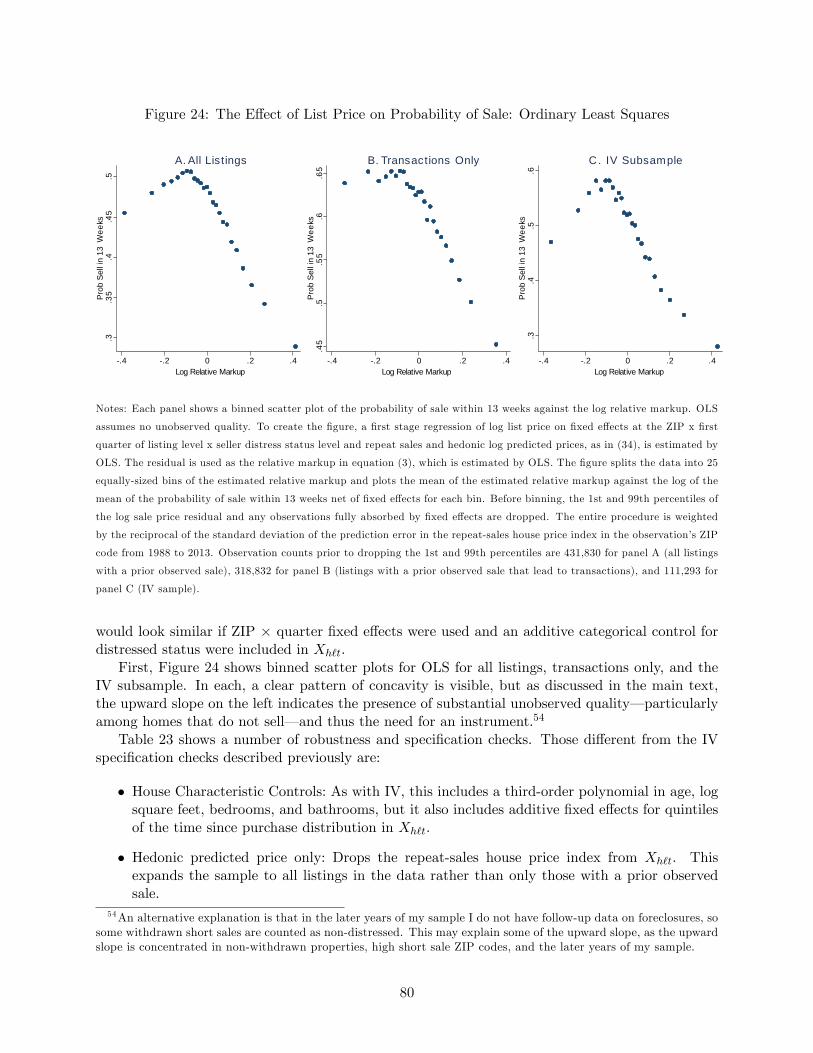
Figure 24: The E¤ect of List Price on Probability of Sale: Ordinary Least Squares.3

.35

.4.4

5.5

Pro

b S

ell i

n 13

Wee

ks

­.4 ­.2 0 .2 .4Log Relative Markup

A. All Listings

.45

.5.5

5.6

.65

Pro

b S

ell i

n 13

Wee

ks

­.4 ­.2 0 .2 .4Log Relative Markup

B. Transactions Only

.3.4

.5.6

Pro

b S

ell i

n 13

Wee

ks

­.4 ­.2 0 .2 .4Log Relative Markup

C. IV Subsample

Notes: Each panel shows a binned scatter plot of the probability of sale within 13 weeks against the log relative markup. OLS

assumes no unobserved quality. To create the �gure, a �rst stage regression of log list price on �xed e¤ects at the ZIP x �rst

quarter of listing level x seller distress status level and repeat sales and hedonic log predicted prices, as in (34), is estimated by

OLS. The residual is used as the relative markup in equation (3), which is estimated by OLS. The �gure splits the data into 25

equally-sized bins of the estimated relative markup and plots the mean of the estimated relative markup against the log of the

mean of the probability of sale within 13 weeks net of �xed e¤ects for each bin. Before binning, the 1st and 99th percentiles of

the log sale price residual and any observations fully absorbed by �xed e¤ects are dropped. The entire procedure is weighted

by the reciprocal of the standard deviation of the prediction error in the repeat-sales house price index in the observation�s ZIP

code from 1988 to 2013. Observation counts prior to dropping the 1st and 99th percentiles are 431,830 for panel A (all listings

with a prior observed sale), 318,832 for panel B (listings with a prior observed sale that lead to transactions), and 111,293 for

panel C (IV sample).

would look similar if ZIP � quarter �xed e¤ects were used and an additive categorical control fordistressed status were included in Xh`t.

First, Figure 24 shows binned scatter plots for OLS for all listings, transactions only, and theIV subsample. In each, a clear pattern of concavity is visible, but as discussed in the main text,the upward slope on the left indicates the presence of substantial unobserved quality� particularlyamong homes that do not sell� and thus the need for an instrument.54

Table 23 shows a number of robustness and speci�cation checks. Those di¤erent from the IVspeci�cation checks described previously are:

� House Characteristic Controls: As with IV, this includes a third-order polynomial in age, logsquare feet, bedrooms, and bathrooms, but it also includes additive �xed e¤ects for quintilesof the time since purchase distribution in Xh`t.

� Hedonic predicted price only: Drops the repeat-sales house price index from Xh`t. Thisexpands the sample to all listings in the data rather than only those with a prior observedsale.

54An alternative explanation is that in the later years of my sample I do not have follow-up data on foreclosures, sosome withdrawn short sales are counted as non-distressed. This may explain some of the upward slope, as the upwardslope is concentrated in non-withdrawn properties, high short sale ZIP codes, and the later years of my sample.

80

� Low REO ZIPs: Only includes ZIP codes with less than 20 percent REO sale shares from2008 to 2013. (REO is a sale of a foreclosed property.)

� Low Short ZIPs: Only includes ZIP codes with less than 20 percent short sale shares from2008 to 2013. (A short sale occurs when a homeowner sells their house for less than theiroutstanding mortgage balance and must negotiate the sale with their lender.)

� No REO or Short Sale: Drops REOs, short sales, and withdrawn sales subsequently foreclosedupon homes, thus only leaving non-distressed sales.

� Transactions only: Drops houses withdrawn from the market.

� IV Subsample: Drops homes with negative appreciation since purchase, REOs, and homespreviously purchased with all cash.

All speci�cations show signi�cant concavity.

C.5 Monte Carlo Assessment of Bias From Other Sources of Markup Variation

This appendix presents Monte Carlo simulations to assess the degree of bias from other sources ofvariation in the relative markup entering g (�) nonlinearly.

To do so, for each house in the IV sample I simulate dh`t using an assumed g (�) and an estimated h`t:

dh`t = g (ph`t � ~ph`t) + `t + "h`t.

However, rather than assuming ph`t � ~ph`t = f (zh`t), I let ph`t � ~ph`t = f (zh`t) + �h`t and reportresults for di¤erent parameterizations for the other sources of relative markup variation �h`t.

Speci�cally, I follow a �ve step procedure 1,000 times and report the average values:

1. Based on �rst stage, calculate ph`t � ~ph`t = f (zh`t).

2. Estimate `t given g (�)

3. Draw �h`t. Using the known g (�), calculate g (f (zh`t) + �h`t) + `t

4. dh`t is Bernoulli: a house sells with probability g (f (zh`t) + �h`t) + `t

5. Run the estimator of interest on the simulated data.

Table 24 shows results with a normally distributed �h`t that is independent of f (zh`t). Theassumed g (�) is the third-order polynomial estimate of g (�) shown in Figure 5. Increasing thestandard deviation of �h`t leads to a g (�) that is steeper and more linear than the baseline estimates.Other sources of variation in the relative markup that are independent of the instrument wouldthus likely lead to an under-estimate of the true degree of concavity.

Spurious concavity is, however, a possibility if the variance of �h`t is correlated with zh`t. Specif-ically, consider the case where the instrument captures most of the variation in the relative markupfor sellers with low appreciation since purchase but little of the variation with high appreciationsince purchase. Then the observed probability of sale at low ph`t � ~ph`t would be an average ofthe probabilities of sale at true ph`t � ~ph`ts that are scrambled, yielding an attenuated slope forlow ph`t � ~ph`t. However, at high ph`t � ~ph`t, the observed ph`t � ~ph`t would be close to the trueph`t � ~ph`t, yielding the true slope.

81

Table 24: Monte Carlo Simulations: Other Sources of Markup Variation Independent of Instrument

3-Part Spline SD of �h`tCoef Estimates 0.000 0.01 0.02 0.04Lowest Tercile -0.215 -0.851 -1.110 -2.486

(0.371) (0.571) (0.422) (0.379)Middle Tercile 0.201 -0.768 -1.145 -3.002

(1.037) (1.249) (1.090) (1.008)Highest Terclie -2.219 -1.861 -2.077 -3.386

(0.264) (0.605) (0.816) (0.267)High - Low -2.006 -1.010 -0.968 -0.900

(0.429) (1.068) (1.032) (0.443)

Notes: Each column shows the mean and standard deviation over 1,000 Monte Carlo simulations of the point estimates of

a three-part spline in g(.) as in the main text. The simulated data is the actual data for all parameters except for

whether the house sold within 13 months, which is created as simulated data using an assumed value for g(.), here the

baseline estimate, and then adding noise to the �rst stage relative markup that is independent of the instrument and

normally distributed with mean zero and the indicated standard deviation. The simulation procedure is described in

detail in the Appendix text.

Table 25: Monte Carlo Simulations: Other Sources of Markup Variation Corr With Instrument

SD f (z) < :01 0 0.05 0.5 1.0 0.5SD f (z) � :01 0 0 0 0 0.2Lowest Tercile -1.267 -1.256 -0.557 -.194 -0.566

(0.382) (0.381) (0.414) (.405) (0.404)Middle Tercile -1.556 -1.629 -0.768 -.399 -0.786

(1.008) (1.000) (1.084) (1.070) (1.044)Highest Terclie -1.321 -1.315 -1.454 -1.503 -1.234

(0.263) (0.257) (0.281) (0.275) (0.271)High - Low -0.054 -0.060 -0.897 -1.310 -.668

(0.450) (0.436) (.479) (0.466) (0.454)

Notes: Each column shows the mean and standard deviation over 1,000 Monte Carlo simulations of the point estimates of a

three-part spline in g(.) as in the main text. The simulated data is the actual data for all parameters except for whether the

house sold within 13 months, which is created as simulated data using an assumed value for g(.), here the baseline estimate,

and then adding noise to the �rst stage relative markup. Here the variance of the noise depends on f (zh`t) (the estimatedlog relative markup) and thus the instrument. Speci�cally, the noise is normally distributed with a standard deviation equal

to the �rst row if f (zh`t) < :01 and the second row if f (zh`t) � :01. This makes the noise larger for homes withmore appreciation since purchase, creating the potential spurious concavity from heterskedasticity described in the text. The

simulation procedure is described in detail in the Appendix text.

Table 25 illustrates that this type of bias could cause spurious concavity, but that generating theamount of concavity I observe in the data would require an extreme amount of unobserved variationin the relative markup at low levels of appreciation since purchase. To show this, I assume thetrue g (�) is linear and let the standard deviation of �h`t depend on f (zh`t) as indicated in the �rsttwo rows of the table. The �rst column shows estimates with no noise, which are approximately

82

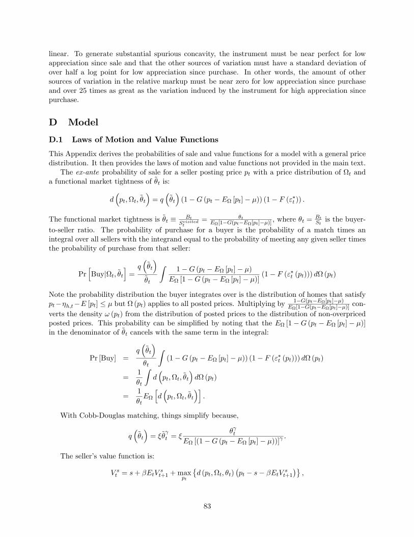
linear. To generate substantial spurious concavity, the instrument must be near perfect for lowappreciation since sale and that the other sources of variation must have a standard deviation ofover half a log point for low appreciation since purchase. In other words, the amount of othersources of variation in the relative markup must be near zero for low appreciation since purchaseand over 25 times as great as the variation induced by the instrument for high appreciation sincepurchase.

D Model

D.1 Laws of Motion and Value Functions

This Appendix derives the probabilities of sale and value functions for a model with a general pricedistribution. It then provides the laws of motion and value functions not provided in the main text.

The ex-ante probability of sale for a seller posting price pt with a price distribution of t anda functional market tightness of ~�t is:

d�pt;t; ~�t

�= q

�~�t

�(1�G (pt � E [pt]� �)) (1� F ("�t )) .

The functional market tightness is ~�t � BtSvisitedt

= �tE[1�G(pt�E[pt]��)] , where �t =

BtStis the buyer-

to-seller ratio. The probability of purchase for a buyer is the probability of a match times anintegral over all sellers with the integrand equal to the probability of meeting any given seller timesthe probability of purchase from that seller:

PrhBuyjt; ~�t

i=q�~�t

�~�t

Z1�G (pt � E [pt]� �)

E [1�G (pt � E [pt]� �)](1� F ("�t (pt))) d (pt)

Note the probability distribution the buyer integrates over is the distribution of homes that satisfypt��h;t�E [pt] � � but (pt) applies to all posted prices. Multiplying by

1�G(pt�E[pt]��)E[1�G(pt�E[pt]��)] con-

verts the density ! (pt) from the distribution of posted prices to the distribution of non-overpricedposted prices. This probability can be simpli�ed by noting that the E [1�G (pt � E [pt]� �)]in the denominator of ~�t cancels with the same term in the integral:

Pr [Buy] =q�~�t

��t

Z(1�G (pt � E [pt]� �)) (1� F ("�t (pt))) d (pt)

=1

�t

Zd�pt;t; ~�t

�d (pt)

=1

�tE

hd�pt;t; ~�t

�i.

With Cobb-Douglas matching, things simplify because,

q�~�t

�= �~�

t = �

� tE [(1�G (pt � E [pt]� �))]

.

The seller�s value function is:

V st = s+ �EtVst+1 +maxpt

�d (pt;t; �t)

�pt � s� �EtV st+1

�,

83

where pt is own price. For a staggered model, in period � = 0 when the seller is choosing price, thevalue function is:

V s;0t = s+ �EtVs;1t+1 +max

p0t

nd�p0t ;t; �t

� �p0t � s� �EtV

s;1t+1

�o,

and in period � 6= 0 when price is �xed, the value function is:

V s;�t = s+ �EtVs;�+1t+1 + d (p�t ;t; �t)

�p�t � s� �EtV

s;�+1t+1

�.

p�t = p��1t�1 and Vs;Nt = V s;0t , so that V s;�+1t+1 corresponds to V s;0t+1 when � = N � 1.

The buyer�s value function integrates out over each type of seller, multiplying the probability ofpurchase from that type of seller by the surplus obtained from purchasing from that type of seller:

V bt = b+ �EtVbt+1 +

1~�t

Zd�pt;t; ~�t

�� V ht � p�t � b� �V bt+1 + "�;�t (p�t )

+E�"� "�;�t (p�t ) j" > "�;�t (p�t )

� � d (pt) .The purchase decisions from each type of seller are optimal, so

"�;�t (p�t ) = p�t + b+ �Vbt+1 � V ht .

Plugging this into V bt gives:

V bt = b+ �EtVbt+1 +

1

�t

Zd�pt;t; ~�t

�E�"� "�;�t (p�t ) j" > "�;�t (p�t )

�d (pt)

= b+ �EtVbt+1 +

1

��t

Zd�pt;t; ~�t

�d (pt) .

Given the setup presented in the main text and summarized in Figure 6, the laws of motion foran arbitrary list price distribution t are:

Bt =

�1� 1

�t�1Et�1

hd�pt�1;t�1; ~�t�1

�i�Bt�1 (35)

+�r�1�K

�k�t�1

��Rt�1 +

�1� LK

�k�t�1

���h�1� C

�c�t�1

��Ht�1 (36)

S =�1� Et�1

hd�pt�1;t�1; ~�t�1

�i�St�1 + �

h�1� C

�c�t�1

��Ht�1 (37)

Ht = Et�1

hd�p�t�1;t�1; ~�t�1

�iSt�1 +

�1� �h

�1� C

�c�t�1

���Ht�1 (38)

Rt =�1� �r

�1�K

�k�t�1

���Rt�1 + LK

�k�t�1

��h�1� C

�c�t�1

��Ht�1. (39)

For staggered pricing there are laws of motion for each S� :

S�t =�1� d

�p��1t�1 ;t�1;

~�t�1��

S��1t�1 8 � 6= 0 (40)

S0t =�1� d

�p��1t�1 ;t�1;

~�t�1��

SN�1t�1 + �h�1� C

�c�t�1

��Ht�1. (41)

84

The value functions for homeowners and renters are,

V ht = h+ �

��h�1� C

�c�t+1

��Et�V st+1 + LV

0 + (1� L)V bt+1�

��hC�c�t+1

�E [cjc < c�t ] +

�1� �h

�1� C

�c�t+1

���EtV

ht+1

�(42)

V rt = u+ xt + �

��r�1�K

�k�t+1

��EtV

bt+1 � �rK

�k�t+1

�E [kjk < k�t ]

+�1� �r

�1�K

�k�t+1

���EtV

rt+1

�, (43)

where xt is the stochastic AR(1) shock to the �ow utility of renting. In the staggered model V st+1is replaced by V s;0t+1. The value functions are standard with the exception of terms for the expectedcost paid by a homeowner and renter if they decide not to enter the housing market, E [cjc < c�t ]and E [kjk < k�t ], respectively.

D.2 Proofs

D.2.1 Lemma 3: Optimal Flexible Price Setting

The seller�s value function is:

V st = s+ �V st+1 +maxp

nd�pt;t; ~�t

� �pt � s� �V st+1

�o.

The seller�s optimal price is de�ned by the �rst order condition:

pt = s+ �V st+1 �d�pt;t; ~�t

�@d(pt;t;~�t)

@pt

,

where d�pt;t;~�t

�is de�ned in equation (12) and "�t = b + �V bt+1 + pt � V ht . The impact of an

individual�s price on E [1�G (pt � E [pt]� �)] is in�nitesimal so,

@d�pt;t; ~�t

�@pt

= �d�pt;t; ~�t

�� f ("�t )

1� F ("�t )+

g ((pt � E [pt]� �))1�G (pt � E [pt]� �)

�,

which gives:

p = s+ �V st+1 +1

f("�t )1�F ("�t )

+ g((pt�E[pt]��))1�G(pt�E[pt]��)

= s+ �V st+1 +1

1�

1

1+exp�� pt�E[pt]��

�

� + � .

For uniqueness, the second order condition is:

@2d�pt;t; ~�t

�@p2t

�pt � s� �V st+1

�+ 2

@d�pt;t; ~�t

�@pt

< 0,

85

or equivalently,

@2d�pt;t; ~�t

�@p2t

<2

d�pt;t; ~�t

�24@d

�pt;t; ~�t

�@pt

352 .This condition holds locally, as

@2d(pt;t;~�t)@p2t

< 0 around the equilibrium price. However, d�pt;t; ~�t

�is not globally concave as illustrated by Figure 7. Because it is convex as pt � E [pt] ! 1, theLemma speci�es that the optimal price is unique on an interval bounded away from pt = 1.Intuitively, there may be an equilibrium with close to no trade due to the non-concavity, but thisequilibrium is assumed away. Numerical simulations show that the local optimum is the globaloptimum for all parameter values considered.

D.2.2 Lemma 4: Optimal Staggered Price Setting

The price-setting seller�s value function is:

V s;0t = maxp

ns+ �V s;1t+1 (p) + d

�p;t; ~�t

��p� s� �V s;1t+1 (p)

�o,

whereV s;�t (p) = s+ �V s;�+1t+1 (p) + d

�p;t; ~�t

��p� s� �V s;�+1t+1 (p)

�,

and V Nt = V 0t . The �rst order condition is:

��1� d

�p;t; ~�t

��Et@V s;1t+1@p

+ d�p;t; ~�t

�Et

241 + @d(p;t;~�t)@p

d�p;t; ~�t

� �p� s� �V s;1t+1 (p)�35 = 0,

where for � < N � 1,

Et@V s;�t (p)

@p= �

�1� d

�p;t; ~�t

��Et@V s;�+1t+1 (p)

@p+d�p;t; ~�t

�Et

241 + @d(p;t;~�t)@p

d�p;t; ~�t

� �p� s� �V s;�+1t+1 (p)�35 ,

and,

Et@V s;N�1t (p)

@p= d

�p;t; ~�t

�Et

241 + @d(p;t;~�t)@p

d�p;t; ~�t

� �p� s� �s;0t+1�35 .

De�ningDjt (p) = Et

"j�1Y�=0

�1� d�

�p;t+� ; ~�t+�

��#d�p;t+j ; ~�t+j

�and substituting

@V s;1t+1

@p ; :::;@V s;N�1t+N�1

@p

into the �rst order condition gives:

N�1X�=0

��D�t (p)Et

241 + @d(p;t+� ;~�t+�)@p

d�p;t+� ; ~�t+�

� �p� s� �V s;�+1t+�+1

�35 = 0.

86

Rearranging gives:

p =

PN�1�=0 �

�D�t (p)Et

"1 +

� @d(p;t+� ;~�t+� )@p

d(p;t+� ;~�t+�)

�s+ �V s;�+1t+�+1

�#PN�1�=0 �

�D�t (p)Et

"� @d(p;t+� ;~�t+� )

@p

d(p;t+� ;~�t+�)

# ,

which, de�ning �t = Et

"� @d(pt;t+� ;~�t+� )

@pt

d(pt;t+� ;~�t+�)

#and '�t = s+ EtV

s;�+1t+�+1 +

1�t, simpli�es to,

p =

PN�1�=0 �

�D�t (p)

�t'

�tPN�1

�=0 ��D�

t (p)�t

.

For uniqueness, that the second order condition is:

Et

8<: ��1� d

�p;t; ~�t

��@2V s;1t+1

@p2� 2� @d(p;t;

~�t)@p

@V s;1t+1

@p

+2@d(p;t;~�t)

@p +@2d(p;t;~�t)

@p2

�p� s� �V s;1t+1 (p)

�9=; < 0;

where

Et@V s;�t (p)

@p= Et

8<: ��1� d

�p;t; ~�t

��@V s;�+1t+1 (p)

@p

+d�p;t; ~�t

�+

@d(p;t;~�t)@p

�p� s� �V s;�+1t+1 (p)

�9=; ;

Et@2V s;�t (p)

@p2= Et

8<: ��1� d

�p;t; ~�t

��@2V s;�+1t+1 (p)

@p2� 2� @d(p;t;

~�t)@p

@V s;�+1t+1 (p)

@p

+2@d(p;t;~�t)

@p +@2d(p;t;~�t)

@p2

�p� s� �V s;�+1t+1 (p)

�9=; ;

and

Et@V s;N�1t (p)

@p= Et

24d�p;t; ~�t�+ @d�p;t; ~�t

�@p

�p� s� �s;0t+1

�35Et@2V s;N�1t (p)

@p2= Et

242@d�p;t; ~�t

�@p

+@2d

�p;t; ~�t

�@p2

�p� s� �s;0t+1

�35 .The second order condition can be rewritten as:

N�1X�=0

���Yj=0

�1� d

�p;t+j ; ~�t+j

��8<: 2@d(p;t+� ;~�t+�)

@p +@2d(p;t+� ;~�t+�)

@p2

�p� s� �V s;�+1t+�+1 (p)

��2� @d(p;t+� ;

~�t+�)@p

@V s;�+1t+�+1

@p

9=; < 0,

87

where,

Et@V s;t+�t+�

@p= Et

t+N�1Xk=t+�

8>>>><>>>>:�k�t��

24 kYj=t+�

�1� d

�p;j ; ~�j

��35 d�p;t+�+k; ~�t+�+k���d�p;t+�+k; ~�t+�+k

�+

@d(p;t+�+k;~�t+�+k)@p

�p� s� �V s;t+�+k+1t+�+k+1 (p)

��9>>>>=>>>>; .

Combining gives

Et

N�1X�=0

���Yj=0

�1� d

�p;t+j ; ~�t+j

��8<:2@d�p;t+� ; ~�t+�

�@p

+@2d

�p;t+� ; ~�t+�

�@p2

�p� s� �V s;�+1t+�+1 (p)

�9=;�Et

N�1X�=0

��

8>>><>>>:2�

@d(p;t+� ;~�t+�)@p

Pt+N�1k=t+� �

k�t��

24 kYj=�

�1� d

�p;j ; ~�j

��35�@d(p;t+�+k;~�t+�+k)

@p

�p� s� �V s;t+�+k+1t+�+k+1 (p)

�9>>>=>>>;

< Et

N�1X�=0

��

8<:2�@d�p;t+� ; ~�t+�

�@p

t+N�1Xk=t+�

�k�t��

24 kYj=�

�1� d

�p;j ; ~�j

��35 d�p;t+�+k; ~�t+�+k�9=; .

This condition must hold for uniquness. As with the �exible case, d�pt;t; ~�t

�is concave locally

but not globally, as illustrated by Figure 7. Because it is convex as pt � E [pt]!1, the Lemmaspeci�es the optimal price is unique on an interval bounded away from pt = 1. Locally, theleft hand side of the �nal condition is negative, while the right hand side is indeterminate. Inall simulations considered, this condition holds, and numerical simulations show that the localoptimum is the global optimum for all parameter values considered.

D.3 Frictionless Model

In the frictionless case (N = 1 for the staggered model, � = 1 for the backward-looking model),the de�nition of an equilibrium simpli�es to:

De�nition 7 Equilibrium with �exible pricing is de�ned by a price pt, purchase cuto¤s "�t , andseller, buyer, homeowner, and renter value functions V st , V

bt , V

ht , and V

rt , entry cuto¤s c

�t and k

�t ,

and stocks of each type of agent Bt, St, Ht, and Rt satisfying:

1. Optimal pricing (15). All sellers set the same price so pt = E [pt]

2. Optimal purchasing decisions by buyers: "�t = pt + b+ �Vbt+1 � V ht

3. Demand curve (12) simpli�es to q (�t) (1� F ("�t ))

4. Optimal entry decisions by homeowners and renters who receive shocks (9) and (10)

5. The value functions for buyers (13), sellers (14), renters (43), and homeowners (42)

6. The laws of motion for all agents (35), (38), (39), and (37).

88

For the reader�s convenience, the simpli�ed general equilibrium system without a shock is repro-

duced below. Note that d�pt;t; ~�t

�= �� [1�G (��)]1� (1� F ("�t )) is plugged in everywhere:

Bt =

�1� 1

�t�1�� t�1 [1�G (��)]

1� (1� F ("�t ))

�Bt�1

+�r�1�K

�k�t�1

��Rt�1 + (1� LK (k�))�h

�1� C

�c�t�1

��Ht�1

St =�1� �� t�1 [1�G (��)]

1� (1� F ("�t ))

�St�1 + �

h�1� C

�c�t�1

��Ht�1

Ht = �� t�1 [1�G (��)]1�

(1� F ("�t ))St�1 +�1� �h

�1� C

�c�t�1

���Ht�1

Rt =�1� �r

�1�K

�k�t�1

���Rt�1 + LK (k

�)�h�1� C

�c�t�1

��Ht�1

V ht = h+ �

"�h�1� C

�c�t+1

�� �V st+1 + LV

0 + (1� L)V bt+1�

��hC�c�t+1

�E�cjc < c�t+1

�+�1� �h

�1� C

�c�t+1

���V ht+1

#V rt = u+ xt + �

��r�1�K

�k�t+1

��V bt+1 � �rK

�k�t+1

�E�kjk < k�t+1

�+�1� �r

�1�K

�k�t+1

���V rt+1

�V bt = b+ �EtV

bt+1 +

�� t [1�G (��)]1�

(1� F ("�t ))��t

V st = s+ �EtVst+1 + ��

t [1�G (��)]

1� (1� F ("�t ))

11�

1

1+exp(�� )+ �

"�t = b+ �EtVbt+1 + p

it � V ht

pt = s+ �EtVst+1 +

11�

1

1+exp(�� )+ �

c�t = V ht ��V st + (1� L)V bt + LV 0t

�k�t = V rt � V btxt = �xt+1 + �, � � N

�0; �2�

�D.4 Backward-Looking Model

The equilibrium of the staggered pricing model is de�ned by De�nition 6. For the reader�s conve-nience, the general equilibrium system is reproduced below.

89

Full Backward-Looking Model

Bt =

�1� 1

�t�1

h�d�pNt�1;t�1;

~�t�1

�+ (1� �) d

�pRt�1;t�1;

~�t�1

�i�Bt�1

+�r�1�K

�k�t�1

��Rt�1 +

�1� LK

�k�t�1

���h�1� C

�c�t�1

��Ht�1

St =�1� �d

�pNt�1;t�1;

~�t�1

�� (1� �) d

�pRt�1;t�1;

~�t�1

��S1t�1 + �

h�1� C

�c�t�1

��Ht�1

Ht = d�pNt�1;t�1;

~�t�1

��St�1 + d

�pRt�1;t�1;

~�t�1

�(1� �)St�1 +

�1� �h

�1� C

�c�t�1

���Ht�1

Rt = (1� �r (1�K (k�)))Rt�1 + LK�k�t�1

��h�1� C

�c�t�1

��Ht�1

V ht = h+ �

24 �h�1� C

�c�t+1

�� hV s;Rt+1 + LV

0 + (1� L)V bt+1i

��hC�c�t+1

�E�cjc < c�t+1

�+�1� �h

�1� C

�c�t+1

���V ht+1

35V rt = u+ xt + �

��r�1�K

�k�t+1

��V bt+1 � �rK

�k�t+1

�E�kjk < k�t+1

�+�1� �r

�1�K

�k�t+1

���V rt+1

�V bt = b+ �EtV

bt+1 +

1

��t

h�d�pNt ;t;

~�t

�+ (1� �) d

�pRt ;t;

~�t

�iV s;Rt = s+ �EtV

s;Rt+1 + d

�pRt ;t;

~�t

� 11�

1

1+exp(� p�E[p]��� )

+ �

"i�t = b+ �EtVbt+1 + p

it � V ht 8 i

d�pit;t; �

�= q (�t)

�1� F

�"i�t��

exp

�� pit�E[p]��

�

�1+exp

�� pit�E[p]��

�

�24� exp

�� pNt �E[p]��

�

�1+exp

�� pNt �E[p]��

�

� + (1� �) exp

�� pRt �E[p]��

�

�1+exp

�� pRt �E[p]��

�

�35

c�t = V ht ��V st + (1� L)V bt + LV 0t

�k�t = V rt � V bt

pNt =pt�2 + pt�3 + pt�4

3+ �

�pt�2 + pt�3 + pt�4

3� pt�5 + pt�6 + pt�7

3

�pRt = s+ �EtV

st+1 +

11�

1

1+exp(� p�E[p]��� )

+ �

E [pt] = �pNt + (1� �) pRt

pt =�d�pNt ;t;

~�t

�pN + (1� �) d

�pRt ;t;

~�t

�pRt

�d�pNt ;t;

~�t

�+ (1� �) d

�pRt ;t;

~�t

�xt = �xt+1 + �, � � N

�0; �2�

�D.5 Staggered Pricing Model

The equilibrium of the staggered pricing model is de�ned by De�nition 5. For the reader�s convenience, thegeneral equilibrium system for two alternating groups of sellers used for most of the simulations without ashock is reproduced below.

90

Full Staggered Price Model

Bt =

�1� 1

�t�1

�S0t�1St�1

d�p0t�1;t�1;

~�t�1

�+S1t�1St�1

d�p1t�1;t�1;

~�t�1

���Bt�1

+�r�1�K

�k�t�1

��Rt�1 +

�1� LK

�k�t�1

���h�1� C

�c�t�1

��Ht�1

S0t =�1� d

�p1t�1;t�1;

~�t�1

��S1t�1 + �

h�1� C

�c�t�1

��Ht�1

S1t =�1� d

�p0t�1;t�1;

~�t�1

��S0t�1

St = S0t + S1t

Ht = d�p0t�1;t�1;

~�t�1

�S0t�1 + d

�p1t�1;t�1;

~�t�1

�S1t�1 +

�1� �h

�1� C

�c�t�1

���Ht�1

Rt = (1� �r (1�K (k�)))Rt�1 + LK�k�t�1

��h�1� C

�c�t�1

��Ht�1

V ht = h+ �

24 �h�1� C

�c�t+1

�� hV s;0t+1 + LV

0 + (1� L)V bt+1i

��hC�c�t+1

�E�cjc < c�t+1

�+�1� �h

�1� C

�c�t+1

���V ht+1

35V rt = u+ xt + �

��r�1�K

�k�t+1

��V bt+1 � �rK

�k�t+1

�E�kjk < k�t+1

�+�1� �r

�1�K

�k�t+1

���V rt+1

�V bt = b+ �EtV

bt+1 +

1

��t

�S0tStd�p0t ;t;

~�t

�+S1t�1St�1

d�p1t ;t;

~�t

��V s;0t = s+ �EtV

S;1t+1 + d

�p0t ;t;

~�t

��p0t � s� �EtV

s;1t+1

�V s;1t = s+ �EtV

S;0t+1 + d

�p1t ;t;

~�t

��p1t � s� �EtV

s;0t+1

�"i�t = b+ �EtV

bt+1 + p

it � V ht 8 i

d�pit;t; �

�= q (�t)

�1� F

�"i�t��

exp

�� pit�E[p]��

�

�1+exp

�� pit�E[p]��

�

�24S0tSt

exp

�� p0t�E[p]��

�

�1+exp

�� p0t�E[p]��

�

� + S1tSt

exp

�� p1t�E[p]��

�

�1+exp

�� p1t�E[p]��

�

�35

E [p] =S0tStp0t +

S1tStp1t

p1t = p0t�1

p0t =

d�p0t ;t; �t

�24 1�

1

1+exp

�� p0t�E[pt]��

�

� + �350B@s+ �EtV s;1t+1 +

11�

1

1+exp

�p0t�E[pt]��

�

!+�

1CA+��1� d

�p0t ;t; �t

��Etd

�p0t ;t+1; �t+1

��24 1

�1

1+exp

�� p0t�E[pt+1]��

�

� + �350B@s+ �V s;0t+2 +

11�

1

1+exp

�p0t�E[pt+1]��

�

!+�

1CAd�p0t ;t; �t

�24 1�

1

1+exp

�� p0t�E[pt]��

�

� + �35

+��1� d

�p0t ;t; �t

��Etd

�p0t ;t+1; �t+1

�24 1�

1

1+exp

�� p0t�E[pt+1]��

�

� + �35

c�t = V ht ��V st + (1� L)V bt + LV 0t

�k�t = V rt � V btxt = �xt+1 + �, � � N

�0; �2�

�91

D.6 Steady State

All three variants of the model share a unique steady state that can be found by equating the value of theendogenous variables across time periods. Steady state values are denoted without t subscripts. Using thefact that a �xed housing stock of mass one and a �xed population in steady state of mass Pop imply:

H + S = 1

B +H +R = N .

The laws of motion and H + S = 1 give:

H =q (�) [1�G (��)]1� (1� F ("�))

q (�) [1�G (��)]1� (1� F ("�)) + �h (1� C (c�))

S =�h (1� C (c�))

q (�) [1�G (��)]1� (1� F ("�)) + �h (1� C (c�)).

The laws of motion along with B +H +R = Pop imply:

R =LK (k�)�h (1� C (c�))

�r (1�K (k�)) H

B =�h (1� C (c�))

q(�)� [1�G (��)]1� (1� F ("�))

H

LK (k�)

�r (1�K (k�)) =(Pop� 1)

�h (1� C (c�))+

(Pop� �)q (�) [1�G (��)]1� (1� F ("�))

:

The steady state value functions are:

V h =h+ ��h (1� C (c�))

�V s + LV 0 + (1� L)V b

�� ��hC (c�)E [cjc < c�]

1� ��1� �h (1� C (c�))

�V r =

u+ ��r (1�K (k�))V b � ��rK (k�)E [kjk < k�]

1� � (1� �r (1�K (k�)))

V b =b+ q(�)

� [1�G (��)]1� (1� F ("�)) 1�1� �

V s =

s+ q (�) [1�G (��)]1� (1� F ("�)) 11�

1

1+exp(�� )+�

1� � .

Finally optimal pricing, optimal purchase decisions, and optimal entry decisions imply:

"� = b+ �V b + p� V h

p = s+ �V s +1

1�

1

1+exp(�� )+ �

c� = V h ��V s + (1� L)V b + LV 0

�k� = V r � V b.

One can plug these equations into those for "�, c�, and k� to get a three equation system with threeunknowns that has a unique solution.

For staggered price variant of the model with N staggered groups of list-price-setting sellers, there area few more variables that require steady state values. Although each group has a di¤erent price, in steadystate p� = p, "� = ", and V s;� = V s 8 � , where variables � are the frictionless steady-state values. The only

92

di¤erence between the two models�steady states, then, is the S� . One can show that:

S� =

h1� q (�) [1�G (��)]1� (1� F ("�))

i�PN�1

j=0

h1� q (�) [1�G (��)]1� (1� F ("�))

ij S,where S is the steady state mass of sellers for the frictionless model. Since all vintages of sellers post thesame price in steady state, this does not a¤ect the three equation system for the frictionless model, whichcontinues to de�ne the steady state for the staggered-pricing model.

For the backward-looking variant of the model, the steady state of the model is identical to the frictionlesscase if pi = p and "i = ", where i = fN;Rg.

D.7 Simulation Details

I present two main types of results: impulse response functions and stochastic simulations. For both, Ireport price, sales volume, months of supply, and buyer and seller entry. This section describes how theseare computed.

Price is the average transaction price in the market. This is a weighted average of prices, where theweights are equal to the share of transactions accounted for by sellers with each price:

pt =

Rpid�pit;t;

~�t

�dtR

d�pit;t;

~�t

�dt

.

For a frictionless model, this is just the common price. For the backward-looking model, this is equal to pt =

�d(pNt ;t;~�t)pN+(1��)d(pRt ;t;~�t)p

Rt

�d(pNt ;t;~�t)+(1��)d(pRt ;t;~�t). For the staggered model, this is equal to pt =

S0tS0t+S

1td(p0t ;t;~�t)p

0t+

S1tS0t+S

1td(p1t ;t;~�t)p

0t

S0tS0t+S

1td(p0t ;t;~�t)+

S1tS0t+S

1td(p1t ;t;~�t)

.

Sales volume is the total amount of sales. This is equal to:

volt = Et

hd�p�t ;t;

~�t

�iSt,

and months of supply is equal to the mass ratio of the mass of sellers to sales volume:

MSt =voltSt

= Et

hd�p�t ;t;

~�t

�i.

Buyer and seller entry come from the laws of motion (35) and (37) and are equal to:

BEntert = �r (1�K (k�t ))Rt + (1� LK (k�t ))�h (1� C (c�t ))Ht

SEntert = �h (1� C (c�t ))Ht.

Buyer entry has two terms re�ecting the entry decisions of renters who receive shocks and new entrants tothe metropolitan area.

For the impulse response functions, I use Dynare to compute the impulse response as the average di¤er-ence between two sets of 100 simulations that use the same sequence of random shocks except for one periodin which an additional standard deviation shock is added. For the entry simulation in Figure 12, I plot theabove values at monthly frequencies form a selected simulation. For Table 8, I run 200 simulations of 500years, collapse the data to quarterly frequency, then calculate the annual change in log price, log volume,and log inventory or estimate the price change on inventory levels regression for each of the 200 simulatedseries. I report the average values in the table.

93

D.8 Understanding Momentum Arising From Staggered Prices

The full dynamic intuition with staggered pricing is more nuanced than the static intuition presented inthe main text because the seller has to weigh the costs and bene�ts of perturbing price across multipleperiods. The intuition is clearest when one considers why a seller does not �nd it optimal to deviate froma slowly-adjusting price path by listing his or her house at a level closer to the new long-run price after aone-time permanent shock to fundamentals.

After a positive shock to prices, if prices are rising slowly why do sellers not list at a high price, sell atthat high price in the o¤ chance that a buyer really likes their house, and otherwise wait until prices arehigher? Search is costly, so sellers do not want to set a very high price and sit on the market for a very longtime. Over a shorter time horizon, the probability of sale and pro�t are very sensitive to perturbing pricewhen a house�s price is relatively high but relatively insensitive to perturbing price when a house�s price isrelatively low. This is the case for two reasons. First, despite the fact that the probability of sale is lowerwhen a house�s price is relatively high, demand is much more elastic and so a seller weights that period�s lowoptimal price more heavily. Second, on the equilibrium path, prices converge to steady state at a decreasingrate, so the sellers lose more buyers today by setting a high price than they gain when they have a relativelylow price tomorrow. Consequently, in a rising market sellers care about not having too high of a price whentheir price is high and do not deviate by raising prices when others are stuck at lower prices.

After a negative shock to prices, if prices are falling slowly and search is costly, why do sellers not deviateand cut their price today to raise their probability of sale and avoid search costs if selling tomorrow meansselling at a lower price? Although the fact that the elasticity of demand is higher when relative price ishigher makes the seller care more about not having too high of a relative price when their price is higher,there is a stronger countervailing e¤ect. Because prices converge to steady state at a decreasing rate on theequilibrium path, sellers setting their price today will undercut sellers with �xed prices more than the sellersare undercut in the future. They thus gain relatively fewer buyers by having a low price when their priceis relatively high and leave a considerable amount of money on the table by having a low price when theirprice is relatively low. On net, sellers care about not having too low of a price when they have the lowerprice and do not deviate from a path with slowly falling prices.

These intuitions in Figure 25, which shows simulation results for the N = 2 case that depict the weightsplaced the optimal �exible price in each period, the optimal �exible price in each period, and the reset price,equal to the weighted average of the optimal �exible prices. The solid blue line corresponds to the period inwhich the price is reset, in which the seller is in the higher priced group, and the dashed red line correspondsto the period after the price is reset, in which the seller is in the lower priced group. Panels A, B, and C arefor an upward shock, while panels D, E, and F are for a downward shock. In Panel A, the weight is muchlarger on the reset period� and a lower optimal reset price� because the elasticity of demand is higher. Theopposite is true in panel D, as the weighting e¤ect works against momentum, which is why momentum inreset prices appears stronger on the upside in the staggered variant of the model. However, the weightinge¤ect is more made up for by the speed of convergence to steady state, which can most clearly be seen inthe asymmetry of the optimal reset price responses in panel E.

Another way of putting these intuitions is that the model features a trade-o¤ between leaving money onthe table when a seller has the relatively low price and gaining more buyers when a seller has the relativelyhigh price. On the upside, since price resetters raise prices more than future price setters and since they caremore about states with more elastic demand, the loss from losing buyers when a resetters have the relativelyhigh price is stronger. On the downside, since price resetters cut prices more than future price resetters, themoney left on the table by having a lower price when their prices are relatively low is stronger.

E Calibration

E.1 Calibration Targets

The aggregate moments and parameters chosen from other papers are:

� A long-run homeownership rate of 65 percent. The homeownership hovered between 64 percent and66 percent from the 1970s until the late 1990s before rising in the boom of the 2000s and fallingafterwards.

94

Figure 25: Understanding Momentum Arising From Staggered Pricing

0 6 12 18 240.1

0.2

0.3

0.4

0.5

0.6

0.7

0.8

0.9

Months

Wei

ght

A. Weights on Each Period Price

Weight on Period 0 PriceWeight on Period 1 Price

0 6 12 18 240.95

1

1.05

1.1

1.15

1.2

1.25B. Optimal Flexible Price in Each Period

Months

Val

ue R

elat

ive 

to In

itial

 Ste

ady 

Sta

tePeriod 0 Flex PricePeriod 1 Flex Price

0 6 12 18 241

1.01

1.02

1.03

1.04

1.05

1.06

1.07

1.08C. Reset Price

Months

Val

ue R

elat

ive 

to In

itial

 Ste

ady 

Sta

te

0 6 12 18 240.1

0.2

0.3

0.4

0.5

0.6

0.7

0.8

0.9

Months

Wei

ght

D. Weights on Each Period Price

Weight on Period 0 PriceWeight on Period 1 Price

0 6 12 18 240.8

0.9

1

1.1

1.2

1.3

1.4

1.5E. Optimal Flexible Price in Each Period

Months

Val

ue R

elat

ive 

to In

itial

 Ste

ady 

Sta

te

Period 0 Flex PricePeriod 1 Flex Price

0 6 12 18 240.94

0.95

0.96

0.97

0.98

0.99

1F. Reset Price

Months

Val

ue R

elat

ive 

to In

itial

 Ste

ady 

Sta

te

Notes: Panels A, B and C show the impulse response to an upward shock and panels D, E, and F show the impulse response to

a downward shock in response to a one-time surprise shock at time zero in a deterministic model solved in Dynare by Newton�s

method. Panels C and F show the optimal reset prices. Because the optimal reset price is a weighted average of the optimal

�exible prices that would prevail in the period the price is reset (period 0) and the period after (period 1), panels A and D

show the weights and panels B and E show the optimal �exible prices for each period. Panels C and F are thus equal to the

sum of the products of the blue lines and dotted red lines in the preceding two panels.

� = 0:8 from the median speci�cation of Genesove and Han (2012). Anenberg and Bayer (2013) �nda similar number.

� L = 0:7 from the approximate average internal mover share for Los Angeles of 0.3 from Anenbergand Bayer (2013), which is also roughly consistent with Wheaton and Lee�s (2009) analysis of theAmerican Housing Survey and Table 3-10 of the American Housing survey, which shows that underhalf of owners rented their previous housing unit.

� A median tenure for owner occupants of approximately nine years from American Housing Survey1997 to 2005 (Table 3-9).

� The approximately equal time for buyers and sellers is from National Association of Realtors surveys(Head et al., 2014; Genesove and Han, 2012). This implies that a normal market is de�ned by abuyer to seller ratio of � = 1. I assume a time to sale in a normal market of four months for bothbuyers and sellers. There is no de�nitive number for the time to sale, and in the literature it iscalibrated between 2.5 and six months. The lower numbers are usually based on real estate agentsurveys (e.g., Genesove and Han, 2012), which have low response rates and are e¤ectively marketing

95

tools for real estate agents. The higher numbers are calibrated to match aggregate moments (Piazzesiand Schneider, 2006). I choose four months, which is slightly higher than the realtor surveys butapproximately average for the literature.

� Price is equal to $750,000. The average log price in the IV sample corresponds to a price of $632,000,so the $750,000 number implies that on average from 2008 to 2013 prices were 16 percent below theirsteady-state level. This is on the conservative side for coastal California where the bust was severeand appears to have overshot the long-run equilibrium. The results are not sensitive to using a slightlylarger number.

� �h and �r are set so renters and homeowners experience a shock every 29 months. According to theAmerican Housing Survey 1997 to 2005 (Table 4-9), approximately 41 percent of renters moved withinthe last year. That translates to a 29 month interval between moves, which I assume are the shocksthat induce renters to consider owning. For homeowners, there is not similar data on considered moves,so I assume the same shock probability as renters. This means that homeowners stay in their homeswhen they receive a shock with higher probability than renters.

� c�, the amount that the marginal homeowner in steady state would pay to avoid moving and stayin their current house, is set equal to the average transaction cost of selling a home from Haurinand Gill (2002). Haurin and Gill use variation in the length of time that one will stay in a locationamong members of the military for whom assignments to a base are known in advance to estimatemoving costs of owner-occupancy in a user cost framework. Haurin and Gill�s preferred number isthree percent of the home�s value and four percent of household earnings. However, I do not havehousehold earnings so I use their alternate estimate of �ve percent of the home�s value. I apply thisto the steady state price, c� = 0:05� 750; 000 = $37; 500.

� k�, the amount the marginal renter in steady state would pay to avoid moving and stay a renter,is set equal to -$20,000 from the imputed tax savings of owner occupancy from Poterba and Sinai(2008). They �nd that the average household with $125,000 to $250,000 in annual income (I choosethis group because their houses are closest in value to average home in my sample) had an annual 2003tax savings of $7,689 from homeownership ($2,703 from the mortgage interest deduction, $1,125 fromproperty tax deduction, and $3,861 from exclusion of imputed rental income). The average renter inmy sample rents for 29 months until the next time they decide to buy or rent, so the total capitalizedvalue of tax savings is just over $18,500 in 2003 dollars, which I adjust to approximately $20,000 in2008-2013.

� A seven percent annual discount rate corresponding to the mean estimated value for housing searchersin Carrillo (2012). The results are not substantially changed by using values between four and 10percent.

There are several parameters I set to reasonable values that do not have an important e¤ect on thedynamics:

� The probability a homeowner purchases a home they inspect in steady state is 0.5. This pins down �.This parameter does not a¤ect the results unimportant and is set so that the probability of a matchis on [0; 1] in the stochastic simulations (with the exception of a few extremely rare circumstances).

� h is set so that the present discounted value of the �ow utility of living in a home is approximately 2/3of its value in steady state, which implies h = $7,500 per month for a $750,000 house. This parameteris a normalization.

Three time series moments are used:

� The persistence of the shock � = 0:99 is chosen to match the persistence of local income shocks fromGlaeser et al. (2013). They estimate an ARMA(1,1) process at the city level net of a city �xede¤ect and linear drift term to back out the shocks that drive housing cycles. Using BEA income dataand Home Mortgage Disclosure Act data on the income of actual home buyers, they �nd an annualpersistence of 0.89, which implies a monthly persistence of 0.99. Their estimated moving averagecoe¢ cient is small.

96

Figure 26: Seller Entry Elasticity

12.5

1313

.514

14.5

Log 

Rea

l Pric

e

3.6 3.8 4 4.2 4.4 4.6Log Seller Entry

Price Elasticity of Seller Entry = 0.878, R­Squared .52

Notes: Seller entry is computed as Entrantst = Sellerst - Sellerst�1 + Salest, with the stock sellers from the Census Vacancy

Survey and sales from the National Association of Realtors. Price is the CoreLogic national house price index adjusted for

in�ation using the CPI and adjusted for seasonality. All data is quarterly from 1976-2013. The regression coe¢ cient of 0.878

is from a regression of log real price on log seller entry.

� A standard deviation of annual log price changes of 0.065 for the real CoreLogic national house priceindex from 1976 to 2013. This is set to match the standard deviation of aggregate prices for homesthat transact collapsed to the quarterly level in stochastic simulations.

� A price elasticity of seller entry of 0.878 based on the CoreLogic, Census, and National Association ofRealtors data from 1976 to 2013. As shown in Figure 26, this relationship is very strong in the data.As mentioned in footnote 42 in the main text, I use this moment as a target for both �c�c and �k�kbecause the stock of buyers is not observed.

Finally, in the calibration to the micro estimates, I use a target of $10,000 for per-period seller �ow costto determine the zero point, which is not precisely estimated in the data and depends on the deadline for asale used. Together with the target value for the price and the discount rate, the target value for the seller�ow cost determines the seller�s markup in steady state, which in turn pins down the location of the averageprice on the demand curve.

The $10,000 target is based on two pieces of evidence from Genesove and Mayer (1997) and Levitt andSyverson (2008):

� Genesove and Mayer show that in their data for Boston condominiums, homes with low equity arelisted four percent higher (on a base of $200,000) and are on the market for 15 percent longer at a100 percent seller loan-to-value ratio relative to an 80 percent seller loan-to-value ratio. They do notreport average time on the market, so I assume my average steady-state time on the market of fourmonths. This implies a one month delay nets the seller $13,333.

� Levitt and Syverson show that realtors in Chicago sell their house for on average $7,600 more andremain on the market for 9.5 days longer. This implies that a one month delay nets the seller $23,000,although some of this may be due to harder work on the part of the realtor.55

55My estimates imply similar numbers� a one percent price increase on a base of $750,000 increases time on the

97

I average these two data points and account for discounting to �nd that the average seller gives up approxi-mately $18,000 to sell one month sooner. Given that the �ow utility of being a homeowner is set to $7,500,I set the �ow utility of being a seller to an even -$10,000. This translates in my calibration into a sellermarkup of $56,500, or roughly 7.5% of the steady-state sales price.

The assumed seller search cost may have an important e¤ect on the degree of momentum in the modelbecause it controls the seller�s degree of impatience. To assess the robustness of the results to this parameter,in Appendix F.4 I present results from a calibration that uses a much smaller assumed seller search cost of$1,450. Although there is somewhat less momentum because sellers are more patient and willing to forgomatching with a buyer today to obtain a higher price in the future, the model still generates signi�cantmomentum.

The 0.4 �gure for the AR(1) coe¢ cient in the backward-looking model is described in the main text.

E.2 Estimation and Calibration Procedure

As described in the text, the estimation and calibration procedure proceeds in two steps. First, I calibrateto the micro estimates. Then I match the aggregate and time series moments.

Calibration To Micro Estimates

The procedure to calibrate to the micro estimates is largely described in the main text. I start with theIV binned scatter plot (pb; db), which can be thought of as an approximation of the demand curve by 25indicator functions after the top and bottom 2.5 percent of the price distribution is dropped. In Figure 5,the log relative markup pb is in log deviations from the average, and I convert it to a dollar amount usingthe average log price in the IV sample. For each combination of �, �, and �, I use equation (25) to calculatethe sum of squared errors:

�bwb�db � d3 month (pb)

�2.

Because the data is in terms of probability of sale within 13 weeks, d3 month (pb) = d (pb)+(1� d (pb)) d (pb)+(1� d (pb))2 d (pb) is the simulated probability a house sells within three months. For the weights wq, I usea normal kernel centered at the average pb with standard deviation equal to the standard deviation of pb toensure I do not over-�t the outliers and consequently over-�t the curvature in the data. I also need to set �t,the multiplicative constant. I do so by minimizing the same sum of squared errors for a given vector of theparameters (�; �; �). I then search over the parameter vector to �nd the (�; �; �) that minimizes the sum ofsquared errors, using 100 di¤erent random starting values.

As mentioned in the main text, I also choose the price that corresponds to the average price in themarket E [p] to match a seller search cost of $10,000 per month. I do so because the zero point in the binnedscatter plot is not precisely estimated. The seller surplus pins down the steady-state markup because insteady state:

p =s

1� � +Markup

��

1� � Pr [Sell] + 1�,

so given the assumed steady-state values for p and Pr [sell] a given s pins down the markup. I then �nd therelative price corresponding to E [p] so that the above calibration procedure matches the implied steady-statemarkup of $56,500.

Matching the Aggregate Targets

To match the aggregate targets in Table 6, I invert the steady state so that 16 parameters can be solvedfor in terms of 16 targets conditional on (�; �; �). I solve this system, de�ned below, conditional on the14 steady-state targets and values for the �nal two target, �c�c and �k�k, which are set equal as describedabove. I then select a value for the standard deviation of innovations to the AR(1) shock ��, run 25 randomsimulations on 500 years of data, and calculate the standard deviation of annual log price changes and the

market by about six to eleven days. My model, however, implies that a one month delay should require a slightlysmaller price change than three times a 10 day delay.

98

entry elasticity in the simulated data. I adjust the target values for �c�c and �� and recalibrate the remainderof the moments until I match the two time series moments. For the backward-looking model, I repeat thisprocedure altering � until the impulse response to the renter �ow utility shock peaks after 36 months.

The calibration procedure is repeated separately for the staggered price and backward-looking variantsof the model. Although the results are similar, the �� needed to match the data is slightly larger in thebackward-looking model due to the additional momentum. While the calibrated values are not the same,although the di¤erences are minor.

The 16 Equation System

Many variables can be found from just a few target values, and I reduce the 16 unknowns to a fourequation and four unknown system. I assume there are Per periods per month for the calibration. Thesystem is de�ned by:

� �, L, , �r , �h, and V 0 to their assumed values. Note that �, �r, and �r are adjusted accordinglybased on the number of periods in a month.

� � = 1 from the equality of buyer and seller time on the market.

� The buyer purchases 1/2 of the time, which implies 1�F ("�) = 12 . Then using the de�nition of d and

� = 1,

� =1

4Per (1�G (��))1� (1� F ("�)):

where [1�G (��)]1� can be found using the calibrated value of and (�; �).

� Given �, one can solve for "� from Pr [Sell] = � exp (��"�) [1�G (��)]1� .

� The homeownership rate in the model, HH+B+R , is matched to the target moment. Plugging in steady-

state values gives:

Homeownership Rate =�r (1�K (k�)) q (�) [1�G (��)]1� (1� F ("�))

�r (1�K (k�)) q (�) [1�G (��)]1� (1� F ("�)) + ��h (1� C (c�))�r (1�K (k�))+LK (k�)�h (1� C (c�)) q (�) [1�G (��)]1� (1� F ("�))

.

The exogenous target value for the probability a homeowner moves in steady state �h (1� C (c�))(which depends on Per), the known value for q (�) [1�G (��)]1� (1� F ("�)) from time to sale insteady state (which depends on Per), and the target value for �r can be used to solve for the value ofK� (k) that matches the target homeownership rate Rate:

K (k�) =1

1 + 1�r

L�Rate�h(1�C(c�))q(�)[1�G(��)]1� (1�F ("�))(1�Rate)q(�)[1�G(��)]1� (1�F ("�))�Rate���h(1�C(c�))

.

� The population Pop can then be solved for from Pop = H +B +R:

Pop =q (�) [1�G (��)]1� (1� F ("�))

q (�) [1�G (��)]1� (1� F ("�)) + �h (1� C (c�))

� 1 +

LK (k�)�h (1� C (c�))�r (1�K (k�)) +

�h (1� C (c�))q(�)� [1�G (��)]1� (1� F ("�))

!.

Again many of the steady-state probabilities depend on Per.

� (1� C (c�)) can be solved for from the assumed value for �h and the probability a homeowner movesin steady state �h (1� C (c�)).

99

� Given targets for K (k�) and C (c�) and target values for c� and k� as well as �c�c and �k�k , theproperties of the uniform distribution can be used to back out �c, c, �k, and k

c = c� � C (c�) (�c� c)k = k� �K (k�)

��k � k

�.

This leaves h, u, b, and s, which are solved for jointly to match the target price and satisfy three equilibriumconditions for steady state:

"� = b+ �V b + p� V h

p = s+ �V s +1

1�

1

1+exp(�� )+ �

c� = V h ��V s + (1� L)V b + LV 0

�k� = V r � V b.

E.3 Additional Calibrated Values

The calibrated values for the backward-looking model are in Table 7 in the main text. The values for thestaggered model are listed in Table 26.

Table 26: Calibrated Parameter Values for Staggered Price Model

Parameter Value Parameter Value Parameter Value� 0.994 �k $407k b -$92.4k

0.800 k -$1,160k s -$9.8k

� 0.506 Pop 1.484 � .0023

�h 0.035 L 0.700 � 3.80

�r 0.035 V 0 $2,606k � 10.47

�c $458k h $7.5k �� 0.311

c -$1,109k u $3.6k � 0.990

F Additional Simulation Results

F.1 Non-Concave Benchmarks

In the main text, I report that without concavity, it would take between 78 and 93 percent backward-lookingsellers to generate a three year impulse response to the renter �ow utility shock. To generate these numbers,I set � = 300 (in thousands of dollars) so that the concavity kicks in so far from any equilibrium that thedemand curve is linear.

I consider two polar cases. In Figure 10 in the main text, I assume that �� which is now the constantsemi-elasticity of demand since there is no concavity� is equal to its value at the average steady-state pricewith concavity, 1

56:5 . Under this calibration, 78 percent backward-looking sellers are needed for a 36-monthimpulse response to the renter �ow utility shock. This calibration assumes that the variance of idiosyncraticpreference is much smaller than I estimate it to be in my model based on the semi-elasticity of demand forrelatively low-priced homes. I use this calibration for the non-concave 26.5 percent backward-looking linesin Figures 10 and 27.

The opposite case I consider is to assume that � is the same as I estimate in the data. This calibrationimplies seller markups are much higher but the distribution of buyer idiosyncratic preference is unchanged.

100

Figure 27: Price Impulse Response Functions: Downward Shock

0 6 12 18 24 30 36­0.025

­0.02

­0.015

­0.01

­0.005

0

Log 

Impu

lse 

Res

pons

e to

 1 S

D S

hock

Months

B. 26.5% Rule of Thumb Model

26.5% Rule of Thumb, Concave26.5% Rule of Thumb, Non­Concave

0 6 12­0.018

­0.016

­0.014

­0.012

­0.01

­0.008

­0.006

­0.004

­0.002

0

Log 

Impu

lse 

Res

pons

e to

 1 S

D S

hock

Months

A. Frictionless and Staggered Models

Staggered and ConcaveStaggered and Non­ConcaveFrictionless and Concave

Notes: Panel A shows the impulse responses to a one standard deviation shock to the �ow utility of renting in the frictionless

model with concave demand, the staggered model with concave demand, and the staggered model without concave demand. For

the model without concave demand, the threshold for being overpriced � is raised to a level that is never reached, the slope of

the demand curve is adjusted to the steady-state slope at the average price in the concave model, the model is recalibrated, and

the standard deviation of the stochastic shock is adjusted so that the impulse response is even with the frictionless and concave

impulse response after a year. Panel B shows the impulse responses to a one standard deviation shock to the �ow utility of

renting in the backward-looking model with and without concavity. Simulated impulse responses are calculated by di¤erencing

two simulations of the model from periods 100 to 150, both of which use identical random shocks except in period 101 in which

a one standard deviation negative draw is added to the random sequence and then computing the average di¤erence over 100

simulations.

Under this calibration, 93 percent backward-looking sellers are needed for a 36-month impulse response tothe renter �ow utility shock.

Both of these numbers are under 100 percent because with all backward-looking sellers, the impulseresponse increases without bound. As the fraction of backward-looking sellers is reduced from 100 percent,mean reversion is introduced into the IRF. Consequently, any amount of momentum can be obtained byreducing the fraction of backward-looking sellers from 100 percent.

F.2 Downward Shock

Figure 27 shows the impulse response to a downward shock directly analogous to Figure 10. For the 26.5-percent backward-looking model in panel B of Figure 10, and the variants of the staggered model withoutmomentum in panel A, the results look very similar to the upward shock. There is, however, a largerprice drop on impact and less momentum for the staggered and concave model. This asymmetry betweenand upward shock and a downward shock occurs because in the staggered pricing model, groups of sellersleapfrog one another each period, as discussed in Appendix D.8. The optimal price is a weighted average ofthe optimal prices in each period, with the weights corresponding to the discounted probability of sale timesthe semi-elasticity of demand. The semi-elasticity of demand� and hence the weight on price� is higher inthe period with a lower price, which helps momentum for an upward shock but works against momentumand causes the larger drop on impact in for a downward shock.

101

F.3 Impulse Responses For All Variables

In the main text, I only show impulse-responses for non-price variables for an upward shock in the 26.5percent backward-looking model in Figure 11. Figures 29, 30, and 31 show the same impulse responses fora downward shock in the 26.5 percent backward-looking model and for an upward and downward shock inthe staggered models.

The downward shock for the backward-looking model looks close to the mirror image of the upward shock.The staggered model, however, looks somewhat di¤erent. While there is still a gradual price response anda shorter-lived but analogous buyer and seller entry response, volume and inventory both spike on impact.This is because prices change more rapidly, so buyers in the market when the shock occurs have a strongincentive to transact today for an upward shock or to wait to buy for a downward shock. While months ofsupply still overshoots, this e¤ect is less substantial and the spike is more prominent.

F.4 Calibration Robustness: Lower Seller Search Cost

The calibration procedure assumes a seller search cost of $10,000 per month based on �gures from two papers.This assumed parameter is important for the degree of ampli�cation of momentum in the model because itcontrols the degree to which sellers are willing to forgo a higher price in the future in order to attract buyerstoday. To assess the robustness of the results to this important assumed parameter, this section presents acalibration with a far smaller seller search cost of $1,450.

To do so, I use the calibration procedure detailed in Appendix E but change the assumed seller searchcost to $1,450. This results in similar parameter values for most variables except �, which is smaller as thecalibration procedure shifts the average price further into the elastic region of the demand curve.

The results are shown in Figure 28. Two months of staggered pricing leads to an impulse response withseven to eight months of momentum instead of 10 months in the baseline calibration. The variant of themodel with backward-looking sellers generates a three-year impulse response with 37.5 percent of backward-looking sellers, rather than 26.5 percent in the baseline calibration. Thus while using a smaller assumedseller search cost does reduce the degree of momentum generated by the model, the calibrated model stillgenerates substantial ampli�cation of the underlying shock with a much smaller seller search cost.

F.5 Deterministic Impulse Responses For Staggered Model

To show that my results are not due to error in the log-cubic approximation pruning higher order terms usedin the stochastic simulations, Figure 32 shows the impulse response to an upward and downward unexpectedone-time deterministic shock solved exactly by Newton�s method for the staggered model. These impulseresponses look similar to their stochastic counterparts.

102

Figure 28: Impulse Responses For Calibration With Low Seller Search Cost

0 6 12 18 24 30 360

0.02

Log 

Impu

lse 

Res

pons

e to

 1 S

D S

hock

Months

0

0.05

Log 

AR

(5) 

Impu

lse 

Res

pons

e in

 Dat

a

B. 37.5% Backward Looking Model and CoreLogic Data

37.5% Backward Looking, Concave37.5% Backward Looking, Non­ConcaveCoreLogic HPI

0 6 120

0.002

0.004

0.006

0.008

0.01

0.012

0.014

0.016

0.018

0.02

Log 

Impu

lse 

Res

pons

e to

 1 S

D S

hock

Months

A. Frictionless and Staggered Models

Staggered and ConcaveStaggered and Non­ConcaveFrictionless and Concave

Notes: This Figure is the analogue of Figure 10 in the main text using a lower seller search cost for the calibration. Panel A

shows the impulse responses to a one standard deviation negative shock to the �ow utility of renting in the frictionless model

with concave demand, the staggered model with concave demand, and the staggered model without concave demand. For the

model without concave demand, the threshold for being overpriced � is raised to a level that is never reached, the slope of the

demand curve is adjusted to the steady-state slope at the average price in the concave model, the model is recalibrated, and

the standard deviation of the stochastic shock is adjusted so that the impulse response is even with the frictionless and concave

impulse response after a year. Panel B shows the impulse responses to a one standard deviation shock to the �ow utility of

renting in the backward-looking model with and without concavity. For the model without concave demand, the threshold for

being overpriced � is raised to a level that is never reached, the slope of the demand curve is adjusted to the steady-state

slope at the average price in the concave model, and the model is recalibrated. Also shown in panel B in the dotted black line

and with grey 95% con�dence intervals and on the right axis is the impulse response to a one standard deviation price shock

estimated from a quarterly AR(5) for the seasonally and CPI adjusted CoreLogic national house price index for 1976-2013, as

in Figure 1. Simulated impulse responses are calculated by di¤erencing two simulations of the model from periods 100 to 150,

both of which use identical random shocks except in period 101 in which a one standard deviation negative draw is added to

the random sequence, and then computing the average di¤erence over 100 simulations.

103

Figure 29: Impulse Responses to Downward Shock in the Rule-of-Thumb Model

0 6 12 18 24 30 36­0.025

­0.02

­0.015

­0.01

­0.005

0

Log 

Impu

lse 

Res

pons

e to

 1 S

D S

hock

Months

B. 26.5%  Backward Looking Model

26.5% Bac kward Look ing, Concave26.5% Bac kward Look ing, Non­Concave

0 6 12­0.018

­0.016

­0.014

­0.012

­0.01

­0.008

­0.006

­0.004

­0.002

0

Log 

Impu

lse 

Res

pons

e to

 1 S

D S

hock

Months

A. Frictionless and Staggered Models

Staggered and Concav eStaggered and Non­ConcaveFric tionles s  and Conc ave

Notes: Each panel plots the indicated impulse response to a one standard deviation downward shock for the frictionless and

backward-looking variants of the model. The frictionless model uses the same calibration and shock as the 26.5 percent

backward-looking model with no backward-looking sellers. Simulated impulse responses are calculated by di¤erencing two

simulations of the model from periods 100 to 150, both of which use identical random shocks except in period 101 in which

a one standard deviation negative draw is added to the random sequence and then computing the average di¤erence over 100

simulations.

Figure 30: Impulse Responses to Downward Shock in the Rule-of-Thumb Model

0 6 12 18 240

0.002

0.004

0.006

0.008

0.01

0.012

0.014

0.016

0.018

Months

Log 

Dev

iatio

n F

rom

 Ste

ady 

Sta

te

A. Average Price

0 6 12 18 240

0.005

0.01

0.015

0.02

0.025B. Sales Volume

Months

Log 

Dev

iatio

n F

rom

 Ste

ady 

Sta

te

0 6 12 18 24­0.025

­0.02

­0.015

­0.01

­0.005

0C. Months of Supply

Months

Log 

Dev

iatio

n F

rom

 Ste

ady 

Sta

te

0 6 12 18 240

0.005

0.01

0.015

0.02

0.025D. Buyer and Seller Entry

Months

Log 

Dev

iatio

n F

rom

 Ste

ady 

Sta

te

Staggered and ConcaveFrictionless and Concave

Buyer, Staggered and ConcaveSeller,Staggered and ConcaveBuyer, Frictionless and ConcaveSeller, Frictionless and Concave

Notes: Each panel plots the indicated impulse response to a one standard deviation upward shock for the frictionless and

staggered variants of the model. The frictionless model uses the same calibration and shock but all sellers set their price

simultaneously. Simulated impulse responses are calculated by di¤erencing two simulations of the model from periods 100 to

150, both of which use identical random shocks except in period 101 in which a one standard deviation negative draw is added

to the random sequence and then computing the average di¤erence over 100 simulations.

104

Figure 31: Impulse Responses to Downward Shock in the Rule-of-Thumb Model

0 6 12 18 24­0.018

­0.016

­0.014

­0.012

­0.01

­0.008

­0.006

­0.004

­0.002

0

Months

Log 

Dev

iatio

n F

rom

 Ste

ady 

Sta

te

A. Average Price

0 6 12 18 24­0.025

­0.02

­0.015

­0.01

­0.005

0B. Sales Volume

Months

Log 

Dev

iatio

n F

rom

 Ste

ady 

Sta

te0 6 12 18 24

0

0.005

0.01

0.015

0.02

0.025C. Months of Supply

Months

Log 

Dev

iatio

n F

rom

 Ste

ady 

Sta

te

0 6 12 18 24­0.025

­0.02

­0.015

­0.01

­0.005

0D. Buyer and Seller Entry

Months

Log 

Dev

iatio

n F

rom

 Ste

ady 

Sta

te

Staggered and ConcaveFrictionless and Concave

Buyer, Staggered and ConcaveSeller,Staggered and ConcaveBuyer, Frictionless and ConcaveSeller, Frictionless and Concave

Notes: Each panel plots the indicated impulse response to a one standard deviation downward shock for the frictionless and

staggered variants of the model. The frictionless model uses the same calibration and shock but all sellers set their price

simultaneously. Simulated impulse responses are calculated by di¤erencing two simulations of the model from periods 100 to

150, both of which use identical random shocks except in period 101 in which a one standard deviation negative draw is added

to the random sequence and then computing the average di¤erence over 100 simulations.

Figure 32: Response to One-Time Deterministic Shock (Non-Approximated)

0 6 12 18 241

1.01

1.02

1.03

1.04

1.05

1.06

1.07

1.08

Months

Valu

e Re

lativ

e to

 Initia

l Ste

ady S

tate

A. U pw ard  D eterminis tic  Shoc k

StaggeredFr ic tionles s

0 6 12 18 240.94

0.95

0.96

0.97

0.98

0.99

1B. D ow nw ard Shoc k

Months

Valu

e Re

lativ

e to

 Initia

l Ste

ady S

tate

Notes: Each panel plots the value of the indicated variable divided by its initial steady-state value in response to a -.3

deterministic permanent shock to u (roughly consistent with one standard deviation stochastic shock) in the upward panel anda .3 deterministic shock in the downward panel. The frictionless model uses the same calibration and shock but all sellers set

their price simultaneously. Both are solved exactly by Newton�s method assuming that the model returns to steady state in

500 years and use the same calibration as the stochastic staggered model, and the frictionless model includes no staggering.

105