the carbon footprint of electricity from biomass
TRANSCRIPT

The Carbon Footprint of Electricity from Biomass
A Review of the Current State of Science and Policy
June 11, 2012
AUTHORS
Jeremy Fisher, PhD
Sarah Jackson
Bruce Biewald

Table of Contents
1. EXECUTIVE SUMMARY .................................................................................................... 1
2. INTRODUCTION ................................................................................................................. 3
A. DIVERGING OPINIONS ..................................................................................................... 3
B. THE ATTRACTION OF A BIOENERGY ECONOMY .............................................................. 5
C. BIOENERGY USE TODAY, TOMORROW, AND THE FUTURE ............................................. 6
Today 6
Tomorrow 8
A Bioenergy Future? 9
The Big Deal 10
3. BIOENERGY, LAND USE, AND DISPLACED EMISSIONS: A PRIMER................ 11
A. FROM FIELD TO GENERATOR: HARVEST, TRANSPORT, AND PROCESSING ................. 12
B. STACK EMISSIONS ........................................................................................................ 13
C. THE CARBON BALANCE OF ECOSYSTEMS .................................................................... 15
D. NEW PRODUCTION: THE CARBON BALANCE OF NEW PRODUCTION FORESTS OR CONVERSION
TO AGRICULTURE .................................................................................................................. 17
E. INTENSIFIED PRODUCTION: THE CARBON BALANCE OF INCREASING PRODUCTION ..... 18
F. DIVERTED PRODUCTION & LEAKAGE: THE CARBON BALANCE OF SHIFTING FROM PRODUCTS
TO BIOENERGY ..................................................................................................................... 19
Leakage 20
G. RESIDUAL HARVESTING: THE CARBON BALANCE OF REMOVING FORESTRY RESIDUALS21
H. AFFORESTATION: THE CARBON BALANCE OF PLANTING NEW MANAGED FORESTS ...... 22
I. SUSTAINABLE FORESTRY ............................................................................................. 23
J. DISPLACED EMISSIONS ON THE OPERATING AND BUILD MARGINS ............................. 24
K. NON-GHG EMISSIONS ................................................................................................. 25
4. A REVIEW OF EXISTING ACCOUNTING FRAMEWORKS ..................................... 27
A. IMPLICIT OR EXPLICIT CARBON NEUTRALITY ................................................................. 27
B. LIFE CYCLE ANALYSIS .................................................................................................. 28
Processing Emissions 29
Land Use Change and Leakage 30

Avoided Fossil Fuel Use 30
Comparing LCA Results 31
C. TEMPORAL LAG ESTIMATION ........................................................................................ 31
D. GREENHOUSE GAS VALUE ........................................................................................... 33
E. ANNUAL ACCOUNTING .................................................................................................. 34
Policies that have adopted an annual or line-item accounting framework 35
5. IMPLICATIONS ................................................................................................................. 37
A. IMPLICIT OR EXPLICIT CARBON NEUTRALITY ................................................................. 37
New Production Risk 37
Diverted Production Risk 38
Implications of Carbon Neutrality in Policy 40
B. LIFE CYCLE ANALYSIS .................................................................................................. 42
Inconsistent system boundaries or basis assumptions 42
Inconsistent framework with other energy sources 43
C. GREENHOUSE GAS VALUE ........................................................................................... 43
D. TEMPORAL LAG ESTIMATION ........................................................................................ 44
6. ANNUAL ACCOUNTING: A FEASIBLE REGULATORY MECHANISM ................ 45
A. THE EPA PROPOSED ANNUAL FRAMEWORK ............................................................... 45
Distinguish “good” and “bad” actors 47
B. A CONSISTENT FRAMEWORK ........................................................................................ 47
C. THE VALUE OF A PRECAUTIONARY APPROACH ............................................................ 48
7. APPENDIX A: BIOENERGY CARBON NEUTRALITY IN CURRENT FRAMEWORK AND
POLICIES ...................................................................................................................................... 49
8. APPENDIX B: DISPLACED EMISSIONS ON THE OPERATING AND BUILD MARGINS
53
Displaced Emissions on the Operating Margin 53
Displaced Emissions on the Build Margin 53
9. APPENDIX C: COMMENTS ON EPA ANNUAL ACCOUNTING FRAMEWORK .. 55
10. REFERENCES................................................................................................................... 57

The Carbon Footprint of Electricity from Biomass
▪ 1
1. Executive Summary
In the US electric sector, biomass energy accounts for only about 1.5% of total generation and has
seen little growth in the past two decades. However, some forecasts assert that the use of
biomass for energy purposes could rise significantly in coming years under policies to promote
renewable energy; a recent study from the US Department of Energy forecasts that consumption
of forest biomass could double by 2030, and a some research suggests that the US alone could
see large tracts of land in biomass energy production by mid or end of the century under a CO2
policy scenario, a future that would use the equivalent of about 75% of today’s agricultural area
(e.g. Gurgel et al., 2008). Other forecasts see fairly little growth in biopower in the US. (e.g. Bird
et al., 2010)
The attraction of a biomass electricity economy is substantial: the desire to diversify the power
sector fuel supply; to create rural economic development; to deal with agricultural and forestry
waste streams; to reduce carbon emissions; its similarity to traditional, dispatchable steam
generation technology; and to create opportunities in regions with limited solar, wind, or
geothermal alternatives.
However, a component of the interest in a biomass energy economy rides on the fundamental
precept that bioenergy is either carbon neutral, or at least significantly beneficial. This paper
focuses on dissecting that precept and assumption, in order to bring about a greater
understanding of the factors that influence how one views and measures the carbon footprint of
electricity from biomass. Note that this paper focuses exclusively on woody biomass use for
electricity production, although there are many common threads between the uses of biomass for
energy, generally.
This paper identifies at least five different elements that could be counted in the estimate of the
greenhouse gas footprint of biomass energy:
Direct land use change (LUC and uptake): Changes (either positive or negative) in the
carbon stock of the land used to grow the feedstock that is also attributable to the harvest
of that feedstock.
Harvesting, Transport, and Processing (lifecycle): Emissions released by equipment
during the harvest, transport, and preparation of biomass, including heat and pressure for
drying, pellet formation, torrefaction, chipping, and or shredding.
Stack emissions: Emissions of greenhouse gasses that emerge from the combustion
source.
Displaced emissions: Changes of emissions from existing or planned generators
brought about by the implementation of a bioenergy program or facility.
Indirect land use (leakage): Changes in other landscapes (usually losses) remote from
the feedstock source that are altered due to the market pressure of diverting feedstock to
bioenergy.
Whether to count these elements, and how, is of crucial importance. It is also hotly debated.
Proponents, opponents, researchers, policymakers, and commentators use a variety of
mechanisms to define carbon emissions; there is a great deal of disagreement on which

The Carbon Footprint of Electricity from Biomass
▪ 2
emissions should be considered within an analysis, and which should be considered irrelevant or
burdensome.
This paper gathers the range of assertions, assumptions, and frameworks used in current and
influential papers—including research, grey literature, and established policy—and reviews those
assumptions. We then review the implications of those assumptions and postulate which types of
assumptions might lead to unintended consequence if implemented in full.
As a result of this analysis, we conclude that there is room in the electricity generation sector for
biomass energy as a greenhouse gas mitigation tool. However, to effectively reduce greenhouse
gas emissions, biomass facilities should be subject to a clear and rigorous accounting framework
that results in estimates of greenhouse gas emissions consistent with other energy resources. The
incentives offered to biomass generation, if targeted towards greenhouse gas reductions (implicitly
or explicitly) should be indexed to the outcome of this accounting mechanism. While this paper
focuses largely on the utilization of previously unmanaged forests for woody biomass production,
the accounting frameworks discussed here would also apply to the conversion of additional land
types (such as cropland or grassland) to woody biomass production, or the use of other
feedstocks such as agricultural residue or dedicated bioenergy crops such as switchgrass.
Using an internally and externally consistent framework for counting emissions from bioenergy will
be critical for both system planning and policy. A consistent carbon accounting framework would
be independent of forestry practices is general, but good carbon outcomes will likely require good
forestry practices as well as efficient conversion and use of biomass energy. There are significant
risks in defining, a priori, the emissions benefits (or impacts) of bioenergy; but a consistent
framework will allow regulators and policymakers to determine how large a role biomass energy
should play in a growing renewable energy market.

The Carbon Footprint of Electricity from Biomass
▪ 3
2. Introduction
The research literature on the feasibility, economics, and carbon and land use impacts of biomass
energy (bioenergy) is extensive. The Intergovernmental Panel on Climate Change (IPCC) recently
completed a survey of renewable energy potentials, barriers, and environmental impacts (IPCC,
2011), and cites about 700 sources in the biomass energy chapter alone. Yet the literature is not
unified on a standard mechanism by which to estimate the greenhouse gas (GHG) footprint of
biomass energy, nor is there consensus on whether or not such a footprint even exists. Even
within the extensively authored and reviewed IPCC publication, there is no singular mechanism
proposed to ultimately count emissions from biomass energy, and the section within the
publication that comes closest to laying out a single set of values includes caveats that would not
satisfy the range of researchers and policymakers working on this issue today. The result of these
limitations and choices has been the production of as many or more papers that review the GHG
implications of biomass as those that carry out fundamental research.1 Because of the extensive
cross-sector implications of biomass energy, researchers often limit their analyses to particular
aspects of the energy cycle; it is the “boundary conditions” on these analyses, rather than the
fundamental science itself, that provide only a partial view of bioenergy impacts.
In light of this fact, and the import of one’s choice of assumptions on study results, this paper aims
to review and dissect the boundary conditions and analytical elements that are used to define the
greenhouse gas implications of biomass energy. Note that this paper focuses exclusively on
biomass use for electricity production (i.e., biopower), and is primarily concerned with woody
biomass use, although there are many common threads between the uses of biomass for energy,
generally.2
This paper is not scoped to review the full range of biomass energy proposals, the technology, the
feasibility, or even the economics of the numerous available mechanisms for obtaining useable
energy from biogenic materials. Rather, the purpose of this paper is to gather the range of
assertions, assumptions, and frameworks used in current and influential papers—including
research, grey literature, and established policy—and to review those assumptions.
A. Diverging Opinions
Sedjo (2011) draws attention to two letters from 200 current and former academics in ecology,
forestry, earth and climate sciences, and materials science. These letters were addressed to the
US Congress and Senate in mid-2010 addressing biogenic carbon accounting in the US EPA’s
“Tailoring Rule,” the first regulation to require permits for stationary source greenhouse gas
emissions. The letters, replicated in Sedjo (id.), take diametrically opposed views regarding the
greenhouse gas impacts of bioenergy.
1 A recent review of “life cycle” GHG emissions from biomass-fired electricity from the US National Renewable
Energy Laboratory (NREL, 2011) noted that of 370 pooled references on bioenergy, only 57 were peer reviewed, used “true LCA [life cycle analysis] methods,” were numerically reported, and did not duplicate prior publications. 2 Literature examining other forms of biomass energy, such as liquid fuels, are cited as well for specific questions,
points, or concerns.

The Carbon Footprint of Electricity from Biomass
▪ 4
The first letter, authored by nearly 90 ecologists, argues for “proper accounting,” stating that “any
legal measure to reduce greenhouse gas emissions must include a system to differentiate
emissions from bioenergy based on the source of the biomass.”
The second letter, authored by over 110 foresters, argues that “equating biogenic carbon
emissions with fossil fuel emissions, such as contemplated in the EPA Tailoring Rule and other
policies, is not consistent with good science and, if not corrected, could stop the development of
new emission reducing biomass energy facilities.”
These views, although dramatically simplified in these statements, represent the bookends of a
contentious spectrum. On one side, ecologists—many of whom have made careers studying
terrestrial carbon fluxes, ecosystem responses to global climate change, and the impacts of land
use on carbon balance—express a fundamental need for precaution in the face of a rapidly
evolving desire for low-cost, low-carbon energy sources. The foresters, many of whom are deeply
familiar with sustainable forestry practices and the economics of forestry, see the precaution as a
significant barrier to implementing viable renewable energy technology in today’s energy
landscape.
Many of the authors of these letters appear in our references; these authors are the community
studying bioenergy potential, feasibility, cost, and atmospheric implications. These voices are
often the most outspoken and represent the opinion leaders on both sides of the issue. It is nearly
impossible to review the various frameworks and opine about advantages and shortcomings
without treading on one camp or the other.
In preparing this review, we have attempted to stay open to concerns and issues expressed by
both the ecologists and foresters. The first draft of this paper was reviewed by proponents of both
views, and all parties found that it did not represent their views sufficiently. In this revision, we
attempt to characterize all mainstream views without bias, and then register our own analysis and
opinion. The purpose of this paper is not to find specific values, but rather to prod at the holes in
various accounting frameworks and suggest pragmatic solutions. This process will inevitably invite
discontent.
To segregate between established science and framework, and our own opinion, this paper is
separated into three separate sections:
First, we establish basic fundamentals of the carbon cycle in biomass energy, land use,
and electricity generation and review how specific changes in each of these mechanisms
could impact GHG implications of biomass energy;
Second, we gather assumptions and frameworks from a variety of influential sources in
the science, advocacy, and policy fields;
Third, we review the implications of those assumptions and postulate which types of
assumptions might lead to unintended consequence if implemented in full.
The carbon implications of biomass energy rely on processes from the local (e.g., availability and
type of biomass within economic reach of a generator) to the global (e.g., competition between
globally traded biogenic products). Therefore, this paper does not attempt to give the value, or
even the range of values, of GHG for biomass energy. However, we do propose elements of
analysis that (in our opinion) should be brought under consideration, and we review a mechanism

The Carbon Footprint of Electricity from Biomass
▪ 5
that (again, in our opinion) could level the playing field and minimize perverse incentives or
unintended consequences.
B. The Attraction of a Bioenergy Economy
Biomass resources are among the oldest and certainly most geographically widespread sources
of energy used in the world today. Biomass has a long and storied history as an energy source for
heating and cooking, is a common heat source for agricultural and forestry industrial processes
today, and has been increasingly touted as one of the “wedges” of mitigation tools that could be
used to reduce the atmospheric burden of carbon dioxide by replacing fossil fuels in both
transportation and electricity production (Pacala and Socolow, 2004). This paper focuses
exclusively on biomass use for electricity production, although there are many common threads
between the uses of biomass for energy, generally. Biomass attracts strong proponents from
numerous perspectives. Proponents cite benefits, including:
Potential negative emissions: Some have pointed out that if combusting biomass can
be considered a carbon-neutral activity, and if these carbon-neutral biomass energy
facilities are coupled with carbon capture and sequestration (CCS), then this energy
resource could not only reduce emissions, but actually draw carbon from the atmosphere
(Azar, 2011).
Known, dispatchable technology: Used for electricity generation, biomass is expected
to primarily be combusted in traditional steam boilers or gasified for use in combined cycle
turbines. As such, there is broad understanding of how to operate these resources and
integrate them into existing electricity grid operations with a very low incremental learning
curve and fairly low capital expense. Use of biomass in steam and gas-fired plants
renders it one of the few dispatchable “renewable” energy technologies. In particular,
unlike traditional wind and solar technologies, these boilers and turbines can be ramped
as required for load, increasing their value for both capacity and energy purposes.
Opportunities in resource-limited regions: In the US and elsewhere, areas that are rich
in biomass availability may also have limited solar, wind, or geothermal alternatives. In the
face of increased public or regulatory pressure to increase renewable energy
requirements, biomass poses an attractive resource, particularly where there are existing
steam boilers (i.e. coal) that can be converted in part or in whole to biomass combustion
(Eisenstat et al, 2009).
Energy security: Biomass has often been described as a local resource that, primarily for
economic reasons, is unlikely to be transported long distances (see Mann and Spath,
2001; BRDB, 2008). Several authors have postulated an energy security benefit of using
biomass rather than imported fossil fuels (Sathre and Gustavsson, 2009; Koonin, 2006;
US DOE, 2004).3
3 The issue of energy security will not be considered in this paper. However, it is worth noting that others have
expressed concern that in exchange for energy security, the use of biomass energy risks food security in substituting energy for food crops (see Schmidhuber in Petersson and Törnquist-plewa, 2008).

The Carbon Footprint of Electricity from Biomass
▪ 6
Ancillary benefits: At the small scales typical of current practice, biomass is commonly
used to provide benefits independent of energy production, including the disposal of
agricultural wastes. Others have suggested that consuming biomass for energy avoids
emissions from landfilling the biomass (Mann and Spath, 2001), promotes forestry health
from thinnings and “residue removal” (Morris, 2008), improves the economics of the
forestry and agricultural sectors (Sedjo and Sohngen, 2009), and could provide job
benefits in rural economies (English et al., 2011).
The potential benefits of a biomass energy economy drive a significant interest in the resource
and technologies. However, a very large component of that interest rides on the fundamental
precept that biomass energy is either carbon neutral or at least significantly beneficial. The
remainder of this paper focuses on dissecting that precept and assumption.
C. Bioenergy Use Today, Tomorrow, and the Future
Today
Humanity has used wood for heating and cooking for thousands of years. In the US, biomass has
been used by a number of different sectors to produce useful energy, most often through co-
generation at industrial wood processing facilities located near sources of forest biomass. (USDA,
2011). These facilities include primary processing mills, which convert roundwood into products
like lumber and wood pulp, and secondary processing mills, which turn primary wood products into
other products such as pallets, furniture, paper, etc. (US DOE, 2011) Many of these facilities use
the residues generated during processing to produce heat and/or electricity, with the pulp and
paper industry meeting most of its energy needs through these wood residues. (Id.)
Historically, biomass feedstocks have contributed only a small percentage of the total energy
consumed in the United States—including electricity, thermal heat recovery, and liquid
transportation fuels, less than 3.5% over the past 30 years (EIA, 2011). Recently, this number has
climbed past 4% —surpassing hydroelectric energy sources—due to the increase in corn ethanol
production, which is being driven by state and federal mandates and incentives to increase biofuel
production (DOE, 2011).
In the US in 2010, nearly 200 million dry tons of biomass were consumed each year for heating or
energy (US DOE, 2011). Of that biomass, 65% was derived from forest sources (Id.). Figure 1,
below illustrates current US consumption of biomass energy by sector:

The Carbon Footprint of Electricity from Biomass
▪ 7
Figure 1. US biomass energy consumption by sector (EIA, 2010)
In the US, space heating in the residential and commercial sectors accounts for about 17% of total
biomass consumption. Nearly all of this is fuel wood. The industrial sector is the largest consumer
of biomass, accounting for 44% of total consumption, with nearly 90% of that consumption coming
from wood and wood waste. Transportation consumes 31% of total biomass energy, primarily from
ethanol blending. Finally, the electric power generators currently represent only a small
percentage of total biomass consumption (8%).
In the US electric sector, biomass energy only accounts for about 1.5% of total generation, and is
derived from a variety of sources, including wood wastes and biomass liquids (primarily
combusted at mills and wood/pulp production facilities), landfill gas, and municipal wastes.
Much of the existing biomass electricity capacity was built in the 1980s, with most of these plants
being between one and thirty megawatts (ORNL, 2011). Recently, generators have begun to
explore the option of co-firing biomass with coal; in 2009, six percent of central biomass4
electricity was produced in this manner (EIA, 2010).. The bulk of biomass electricity is produced in
cogeneration plants and very small facilities using residues and wastes as feedstocks.
4 Defined as electricity only plants and combined heat and power plants whose primary purpose is to sell electricity
to the public, using biogenic municipal waste as well as wood & other biomass as feedstocks.
Space Heating17%
(wood)
Transportation (primarily ethanol
blending)31%
Industrial44%
(90% wood) MSW+Biosolids 60%
Wood - 40%
Electric8%

The Carbon Footprint of Electricity from Biomass
▪ 8
Figure 2. Fuel mix for US electricity sector by net generation (EIA Form 923, 2010). All biomass
represents 1.4% of total generation.
Tomorrow
In the coming years, the use of biomass for energy purposes could rise significantly under policies
to promote renewable energy; legislative mandates like the federal Renewable Fuel Standard
(RFS) and state Renewable Portfolio Standards (RPS) typically allow biopower to participate as a
renewable energy resource, often with no specific qualification for the feedstock source. Under the
federal RFS, ethanol production (a biofuel, not biopower) has increased sevenfold since 2000 (US
DOE, 2011). In the US, states that have previously not had renewable portfolio standards (RPS)
are beginning to examine the feasibility of implementation, and may see biomass as an attractive
option—particularly in states where solar, wind, and geothermal resources are limited, such as in
the Southeast (see e.g. [KY] KREC, 2008; [GA] Brown et al., 2010; [LA] Sutherlin, 2009).
According to the Oak Ridge National Laboratory (ORNL, 2011), there are approximately 2,600
MW of both direct- and co-fired biomass generators in the US today;5 the US DOE lists another
1040 MW in various stages of proposal or construction,6 and a recent study from the DOE
forecasts that consumption of forest biomass could double by 2030, due in large part to an
anticipated tripling of fuelwood use from increased consumption by electric power plants and co-
fire with coal (US DOE, 2011). Modeling a Clean Energy Standard (CES) proposal in the US
5 The EIA (2010) Form 860 data shows 3260 MW of operating generators with a primary fuel of wood, and another
4340 MW of operating generators with a secondary fuel of wood. 6 US DOE: Wood-fired primary or secondary fuel (817 and 222 MW, respectively). Separately, the group
Partnership for Policy Integrity (PFPI) tracks 115 recent and proposed biomass electricity plants (http://www.pfpi.net/biomass-basics-2) while the Forisk Consultancy group estimates 295 new “viable” biomass
electricity, pelletizing, or other fuel processing plants in the pipeline as of April 2012 (http://www.forisk.com/UserFiles/File/WBUS_Free_201204(1).pdf)
Coal
Gas
Nuclear
Hyroelectric
Oil
Geothermal
Solar
Wind Other
Municipal solid waste
Wood and wood waste
Biomass liquids
Energy crops & byproducts Other biomass
solids
Landfill gas

The Carbon Footprint of Electricity from Biomass
▪ 9
Senate, the US EIA estimates a 100-fold increase in biomass co-fire energy by 2021, or a four and
a half fold increase over a reference case (US DOE, 2011, Bingaman Study)7.
In the absence of a significant policy, much slower growth is forecasted by the DOE; the Annual
Energy Outlook 2011 reference case has central biomass electricity production doubling from
about 25 TWh today to 53 TWh in 2020. Few new dedicated biomass facilities are envisioned.
This growth is largely through the increasing utilization of biomass co-fire in existing coal-fired
power plants. While the EIA analysis of the Bingaman policy shows a substantial expansion of
biomass energy, this is not a certainty, and other analyses have shown wind, solar, and
geothermal to play a larger role than biomass.8
A Bioenergy Future?
A great deal of land is required to realize significant energy gains from biomass. Numerous
studies have estimated large scales of energy potential from biomass on a global basis,
amounting to anywhere from about 100 to 500 annual exojoules (EJ) of energy availability
(globally) by 2050, and twice that by 2100 (Fischer and Schrattenholzer, 2001; Smeets et al.,
2004; Hoogwijk et al., 2006; Luckow et al., 2010; Reilly and Paltsev, 2007; Gurgel et al., 2008). On
a relative scale, the United States currently consumes just over 100 EJ of all types of energy
today,9 and the world is estimated to consume about 550 EJ.
10 Extrapolating forward, the world
could be consuming around 1000 EJ annually by 2050 and 1,500 EJ by 2100.11
In theory, if
biomass were fully exploited to the extent envisioned in these studies, biomass could produce
somewhere between 10-50% of energy requirements in 2050, and 13-66% of energy in 2100. In a
brief thought experiment, one researcher postulated how much land would be required to support
this type of energy yield (Azar, 2011). His research suggests that over 500 million hectares of
agricultural land would be required to support 100 EJ in 2050—or about 1.3 times the amount of
farm land area in the US today (USDA, 2007).12
A 2008 paper suggests that the US alone could
see upwards of 300 million hectares in biomass energy production by 2100 under a CO2 policy
scenario, a future that would use the equivalent of about 75% of today’s agricultural area; the
study estimates that agricultural areas would remain largely intact, but that large tracts of natural
forest would be converted to energy crop (Gurgel et al., 2008). Similarly, a review of biomass
energy research (McKinley et al., 2011) finds:
7 Based on EIA’s assumptions, biomass co-fire was an economic way to meet the near term goals of the policy,
particularly given the expiration of the Production Tax Credit (PTC) and Investment Tax Credits (ITC) for wind and solar. Biomass co-fire grows from 1.88 TWh today to 178 TWh in 2020, or about 4.5% of total electricity generation
in 2020. 8 See, for example, an NREL analysis “Impacts of an 80% Clean Energy Standard on the Electricity Generation
Sector “ available at: http://www.rff.org/Documents/Events/Seminars/110727_CES/110727_Steinberg.pdf 9 Total Energy Supply, Disposition, and Price Summary, Reference Case. Consumption (2010). Total Consumption
of liquid fuels, fossil fuels, biomass, and other renewable energy = 97.77 quadrillion btu (Qbtu), or 103 EJ at 0.94 EJ/QBtu. (US DOE EIA, 2011a) 10
EIA IEO 2011. World Total Energy Consumption by Region and Fuel, Reference Case. Total World Consumption (2010) = 522 Qbtu, or 550 EJ. (US DOE EIA, 2011b) 11
World Total Energy Consumption by Region and Fuel, Reference Case. Total World Consumption, linear
extrapolation from 2005 through projected 2035, extrapolated to 2050 (920 Qbtu) and 2100 (1420 Qbtu). 12
Approximately 922,000,000 acres (373,000,000 ha) in 2007. (US DOE EIA, 2011b)

The Carbon Footprint of Electricity from Biomass
▪ 10
…the biological potential for forest sector carbon mitigation is large. Several
studies suggest that using these strategies could offset as much as 10–20%
of current U.S. fossil fuel emissions. To obtain such large offsets in the United
States would require a combination of afforesting up to one-third of cropland
or pastureland, using the equivalent of about one-half of the gross annual
forest growth for biomass energy, or implementing more intensive
management to increase forest growth on one-third of forestland.
Such a dramatic shift would require broad integration across sectors, agreements for agricultural
production and forestry, and large-scale incentives. The diversion of croplands, forestry products,
and even existing non-managed forests could dramatically impact food and wood product prices,
and would likely require a major paradigm shift to a substantive global accounting and regulatory
framework for CO2 sinks and sources, including land use. For example, Wise et al (2009) model
an energy future under a policy scenario in which carbon emissions from land use change do not
fall under the auspices of the policy, in which unmanaged (i.e. natural) forests disappear
completely by 2070. There has been a significant amount of research into this theoretical future,
estimating total energy availability (see Berndes et al., 2003 for a review of studies) and examining
implications on food and energy security (Schmidhuber in Petersson and Törnquist-plewa, 2008)
and the potential for unintended climate consequences (Searchinger et al., 2009; Melillo et al.,
2009). While this long-term theoretical basis is a useful framework, the purpose of this paper is to
examine fundamental assumptions under today’s paradigm of land use, regional and international
trade, and non-unified carbon regulations.
The Big Deal
There is dramatic disagreement about which biomass resources might be used to power a
bioenergy future – for either petroleum-type products or for electricity generation. While the scale
of biomass today is fairly constrained, there are indicators (from both current policy proposals and
new plant proposals) that the sector could blossom with directed energy subsidies or in a carbon-
constrained world, if biomass energy is given a pass as a carbon-neutral resource. As we will
describe in this paper, the atmospheric carbon implications for using some feedstocks (such as
forestry or agricultural residuals and wastes) are very different than others (such as dedicated
energy crops, diverted forestry products, or new forests). An energy policy that promotes biomass
energy, yet does not recognize the carbon dioxide implications of using the resource may result in
large-scale perverse incentives and unintended consequences; a well-designed energy policy with
correct legally/financially binding accounting could produce a reasonable, low carbon energy
resource.

The Carbon Footprint of Electricity from Biomass
▪ 11
3. Bioenergy, Land Use, and Displaced Emissions: a Primer
There are at least five different elements that could be counted in the estimate of the greenhouse
gas footprint of biomass energy (whether to count them, and how, is of crucial importance):
Direct land use change (LUC and uptake): Changes (either positive or negative) in the
carbon stock of the land used to grow the feedstock that is also attributable to the harvest
of that feedstock.
Harvesting, Transport, and Processing (lifecycle): Emissions released by equipment
during the harvest, transport, and preparation of biomass, including heat and pressure for
drying, pellet formation, torrefaction, chipping, and or shredding.
Stack emissions: Emissions of greenhouse gasses that emerge from the combustion
source.
Displaced emissions: Changes of emissions from existing or planned generators
brought about by the implementation of a bioenergy program or facility.
Indirect land use (leakage): Changes in other landscapes (usually losses) remote from
the feedstock source that are altered due to the market pressure of diverting feedstock to
bioenergy.
Figure 3. Possible elements of greenhouse gas accounting for bioenergy. Down arrows represent
sinks or avoided emissions, while up arrows represent emissions (direct and indirect).
Figure 3 shows these basic elements graphically, to be used in schematics later in this paper.
Downward pointing arrows represent sinks and avoided emissions, while the upward pointing
arrows indicate sources of CO2 and other greenhouse gasses to the atmosphere. Uptake
represents the net transfer of carbon into an ecosystem via photosynthesis (balanced by
respiration and disturbances); land use change (LUC) represents changes in the carbon stock of
land by extracting biomass for energy (e.g., conversion of forest to energy crop); life cycle
represents emissions from harvesting, transport, and processing; stack emissions are direct
emissions at the point of combustion; the fossil arrow represents the emissions from fossil power
that might be avoided through biomass energy; finally, leakage refers to land use changes that
occur in a distant location, driven by market forces for diverted biomass products.
These mechanisms are discussed below in relation to bioenergy. In this case, there is more space
given here to a discussion of direct and indirect land use emissions, an area in which there has
LUC
Life
cycl
e
Stac
k
Up
take
Foss
il
Leak
age

The Carbon Footprint of Electricity from Biomass
▪ 12
traditionally been little discussion within the analytical or energy communities, and the subject of
displaced generation and emissions, a particularly important subject in electric system planning
and a contentious topic in considering the potential benefits of biomass energy.
A. From Field to Generator: Harvest, Transport, and Processing
It may require significant energy to transform biomass from standing live plants (or urban wastes)
to a viable generator feedstock. The mechanism used to estimate this energy cost, and the
emissions implications of this transformation are known as life cycle assessments (LCA). LCA
analyses are often highly detailed, specifying all aspects and requirements to grow, harvest,
transport, and process feedstocks, and many include the upstream energy costs of building
harvesting and processing machinery, manufacturing fertilizers and pesticides, and of course,
processing and transporting the fuel to market (see, for example, Mann and Spath, 1997).
All energy sources, from solar to nuclear to fossil fuels, require upstream manufacture and
processing energy and emissions costs; however, these LCA costs are not typically considered in
policy or utility planning, and thus there is a significant question of whether or not these costs
should be considered for biomass energy.
Nevertheless, one of the dominant conversations in the biomass energy community orients around
LCA, the correct system boundaries of LCA, and how overall emissions from biomass combustion
compare to fossil fuel combustion properties. One reason that LCA may dominate the accounting
conversation is because of widespread concern about the processing costs of turning biomass
into liquid fuels (biofuels), which have sometimes been estimated as approximating or exceeding
the energetic costs of production.
On an order of magnitude approximation, studies find about a 5-10% energy penalty associated
with LCA processes (see Mann and Spath, 1997; Forsberg, 2000; Adler et al., 2007), although this
value can be significantly higher for some processing technologies. For example, a brief from the
Penn State Agricultural Research and Cooperative Extension (2009) notes that:
Pellet manufacture requires quite a bit of energy, both for drying damp
feedstock and for running the various pieces of machinery. Large plants
typically burn a portion of their feedstock to provide heat for drying, whereas
smaller facilities often use other means. As a rule of thumb, a pelletizer
requires between 50 and 100 kilowatts of electrical demand for every ton per
hour of production capacity. In addition, electricity is usually needed to
operate any chopping, grinding, drying, cooling, and bagging equipment that
is in use. If a reliable source of electricity is not available, gasoline or diesel-
based equipment is available.
It is not clear from this description if heat for drying or process electricity is included in this
estimate, but using energy content factors from that paper,13
this would imply that pelletizing
operations draw the equivalent of 4-10% of the expected energy output of a generator. Data
13
Heat contents range from 16-20.8 MJ/kg. Assume generator heat rate of 13,000 Btu/kWh.

The Carbon Footprint of Electricity from Biomass
▪ 13
presented in Forsberg (2000), however, suggest that pellet operations draw the equivalent of 570
kWh per MWh of fuel and electricity, or more than half of the embedded energy in the biomass.
LCA differ in the size of the system boundary (i.e. how far upstream or downstream costs and
emissions are estimated), and if the LCA examines the avoided fate of feedstock, land use, or
fossil fuels. Assumptions on avoided emissions from feedstock decomposition, land use (direct
and indirect), and fossil fuel avoidance can be highly influential in the outcome of an LCA. Mann
and Spath (2001) find that greenhouse gas emissions from a co-fire operation may either be less
than or slightly exceed coal-only emissions, depending on assumptions regarding the avoided fate
of biomass residuals used in the operation. Heller et al. (2004) assume that if “willow biomass …
grown specifically for electricity generation” were not used for bioenergy, then the willow would be
landfilled; thus this LCA takes credit for significant avoided methane emissions.
Similarly, assumptions on if direct or indirect land use emissions (discussed below in depth) are
included in the system are highly relevant to the outcome of LCA, but are usually not considered in
LCA (Liska and Cassman, 2008; Anderson-Teixeira, 2011). Many LCA make an implicit or explicit
assumption of land-use carbon neutrality, such as:
CO2 [emissions] from biocombustion is approximately considered to be used
in a closed loop between growing and combustion of biomass” (Forsberg,
2000)
“[biomass] production is considered to be within the power generation system
boundary… [and thus] electricity with… biomass is nearly GHG neutral”
(Heller et al., 2004)
Interpreted, these studies assume that the only factor of land use relevant to GHG is that biomass
grows and sequesters carbon dioxide, and that since this CO2 is released during combustion, the
growth and combustion cycle nets to zero. This critical assumption is explored further in the
sections below.
Finally, assumptions on the avoided use of fossil fuels or avoided fate of fossil fuels can also alter
the outcome of an LCA. Questions regarding the import of the avoided fossil use assumption are
also explored later in this primer.
B. Stack Emissions
Some sources have noted that the direct stack emissions of carbon dioxide from biomass
combustion (i.e. the emissions that exit the stack) exceed the emissions rate of most fossil fuels,
including coal (e.g. Manomet, 2010, Matera, 2000). In a conventional thermal steam generator,
stack emissions from firing biomass would be expected to be greater than fossil fuels because the
energy content of biomass is lower than fossil fuels relative to its carbon content.
The US EPA and Department of Energy (DOE) characterize the carbon content of fuels with an
“emissions factor” in pounds of carbon dioxide (lbCO2) emitted for each embedded unit of energy
(in millions of British thermal units, MMBtu). Coals range from 184-207 lbsCO2/MMBtu, with the
most commonly used bituminous-subbituminous fuels falling at the lower range of this scale
(~184-192, converted to lbs from Quick, 2010) while less common lignites and anthrocites bound

The Carbon Footprint of Electricity from Biomass
▪ 14
the upper end (~194-207, ibid); the resulting emissions from a steam generator with a combustion
heat rate of 11,000 Btu/kWh would range from about 1.01-1.14 tCO2/MWh (see Figure 4, below).
Biomass emissions are not typically reported in the same terms, but an analysis from Jenkins et
al. (1998) contains the carbon content and heating value of various biomass fuels. Translated into
the same units, this content results in emissions factors from 196-254 (median 215
lbsCO2/MMBtu); the same 11,000 btu/kWh generator would emit about 1.18 tCO2/MWh from the
median biomass (willow and poplar result in emissions of 1.19-1.24 tCO2/MWh, respectively).
The higher emissions rate of biomass energy is compounded in part by the current use of biomass
energy in fairly small, less efficient boilers that are able to harness less energy for higher stack
emissions of CO2.The Biomass Energy Data Book (ORNL, 2011) lists over 150 existing biopower
energy plants in the US (as modeled by the IPM model, used by the US EPA) wherein the vast
majority are listed with heat rates around 15,500 Btu/kWh.1415
Using the median emissions factor
for biomass of 215 lbs CO2/MWh, we estimate that stack emissions from existing facilities are
around 1.67 tCO2/MWh, or anywhere from 50-85% higher than emissions from existing coal
plants.
Figure 4. CO2 emissions rates of coal, and biomass at two heat rates
The IPCC recommends that in accounting for CO2 emissions from biomass, either stack emissions
or land use emissions be counted (IPCC, 2006); counting both the emissions that emerge from the
stack and emissions implied by the loss of carbon in standing, live biomass would be counting the
same carbon pool twice (once as it leaves the forest or field, and the second time as it exists the
14
Similarly, the eGRID database lists 65 units that burned exclusively biomass in 2005 and listed wood as a primary fuel type; the average heat rate of these units (weighted by energy output) was approximately 1,522 Btu/KWh. Importantly, the eGRID database does not list CO2 emissions for these generators. 15
Many of these biomass units are cogeneration facilities that can make productive use of the excess heat as a result of the low efficiency conversion to electricity.
0
0.2
0.4
0.6
0.8
1
1.2
1.4
1.6
1.8
2
Coal11,000 btu/kWh
Biomass11,000 btu/kWh
Biomass today15,500 btu/kWh
tCO
2p
er
MW
h

The Carbon Footprint of Electricity from Biomass
▪ 15
stack). Land use emissions are described by changes in the carbon balance of the ecosystems
that supply feedstock for biomass energy facilities, as described below.
C. The Carbon Balance of Ecosystems
Harvesting biomass for energy purposes can directly impact land uses and result in net emissions.
To illustrate the circumstances in which these emissions occur, we establish basic working
principles for natural and managed ecosystems, using a simple forestry example under a variety
of baseline and harvesting conditions.
The rate at which an ecosystem grows (sequesters carbon) and the rate at which it is disturbed
(releasing carbon) dictate the carbon balance of the ecosystem, and where that carbon resides.
Fast-growing forests that are subject to numerous disturbances may hold significant carbon in
fallen trees and litter, while slower-growing forests with infrequent disturbances may hold more
carbon in standing biomass (Frolking et al., 2009). When biomass is felled in natural disturbances
(i.e. through fire, wind, pestilence, or disease), the carbon enters several different “pools”: some
will be immediately transferred to the atmosphere through fire or fast decomposition; some will fall
as leaves, branches, and stems to a litter pool and decay to CO2 (and methane) over seasons to
decades; some will be transferred into organic soils and remain until the soil is disturbed. All of the
carbon that remains on site, either live, dead, or in the soil is, for our purposes, considered
ecosystem carbon.16
Biomass carbon that decomposes or combusts becomes atmospheric
carbon, often in the form of CO2, but also methane, volatiles, and other organic chemicals (Mann
and Spath, 1997).
At small spatial scales of observation (e.g., experimental or observational plots), the carbon
balance of a non-managed forest may appear to go through infrequent large-scale changes (e.g.,
a windstorm destroys a tract of forest every century). However, over larger spatial scales of
observation, the same forest would appear to maintain a fairly steady equilibrium (McKinley et al.,
2011).17
16
This review does not consider the carbon fate of biogenic materials removed for non-energy uses, such as wood products, pulp, or agricultural commodities. Such removals would be considered part of the base case, and are
considered to occur or not occur independently of the requirement for biomass energy. Those products removed from the carbon pool are eventually committed to the atmosphere through decomposition or combustion, but potentially on a different temporal scale then fallen litter. See the ecosystem carbon balance of managed
ecosystems in the sections below. 17
Given constant climate, nutrient, and disturbance regimes.
The Carbon Footprint of Electricity from Biomass
▪ 16
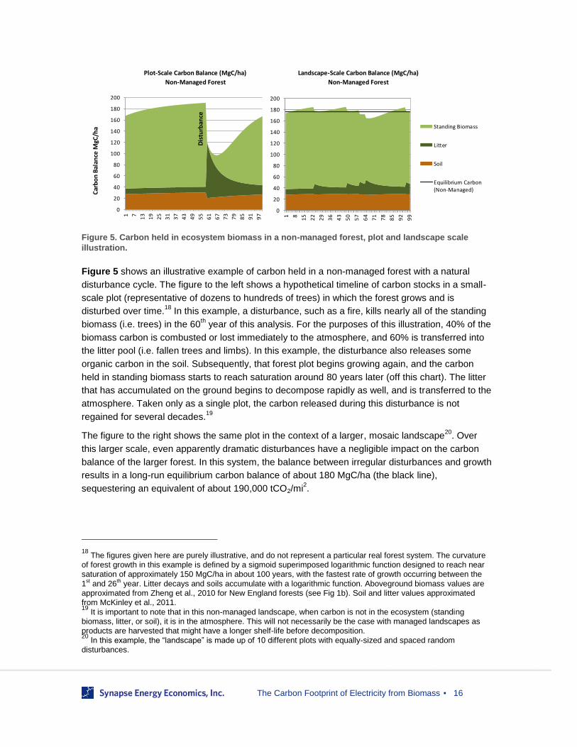
Figure 5. Carbon held in ecosystem biomass in a non-managed forest, plot and landscape scale
illustration.
Figure 5 shows an illustrative example of carbon held in a non-managed forest with a natural
disturbance cycle. The figure to the left shows a hypothetical timeline of carbon stocks in a small-
scale plot (representative of dozens to hundreds of trees) in which the forest grows and is
disturbed over time.18
In this example, a disturbance, such as a fire, kills nearly all of the standing
biomass (i.e. trees) in the 60th year of this analysis. For the purposes of this illustration, 40% of the
biomass carbon is combusted or lost immediately to the atmosphere, and 60% is transferred into
the litter pool (i.e. fallen trees and limbs). In this example, the disturbance also releases some
organic carbon in the soil. Subsequently, that forest plot begins growing again, and the carbon
held in standing biomass starts to reach saturation around 80 years later (off this chart). The litter
that has accumulated on the ground begins to decompose rapidly as well, and is transferred to the
atmosphere. Taken only as a single plot, the carbon released during this disturbance is not
regained for several decades.19
The figure to the right shows the same plot in the context of a larger, mosaic landscape20
. Over
this larger scale, even apparently dramatic disturbances have a negligible impact on the carbon
balance of the larger forest. In this system, the balance between irregular disturbances and growth
results in a long-run equilibrium carbon balance of about 180 MgC/ha (the black line),
sequestering an equivalent of about 190,000 tCO2/mi2.
18
The figures given here are purely illustrative, and do not represent a particular real forest system. The curvature of forest growth in this example is defined by a sigmoid superimposed logarithmic function designed to reach near saturation of approximately 150 MgC/ha in about 100 years, with the fastest rate of growth occurring between the
1st and 26th year. Litter decays and soils accumulate with a logarithmic function. Aboveground biomass values are approximated from Zheng et al., 2010 for New England forests (see Fig 1b). Soil and litter values approximated from McKinley et al., 2011. 19
It is important to note that in this non-managed landscape, when carbon is not in the ecosystem (standing biomass, litter, or soil), it is in the atmosphere. This will not necessarily be the case with managed landscapes as products are harvested that might have a longer shelf-life before decomposition. 20
In this example, the “landscape” is made up of 10 different plots with equally-sized and spaced random disturbances.
Car
bo
n B
alan
ce M
gC/h
a
Landscape-Scale Carbon Balance (MgC/ha)
Non-Managed Forest
Plot-Scale Carbon Balance (MgC/ha)
Non-Managed Forest
0
20
40
60
80
100
120
140
160
180
200
1 7
13
19
25
31
37
43
49
55
61
67
73
79
85
91
97
Standing Biomass
Litter
Soil
Dis
turb
ance
0
20
40
60
80
100
120
140
160
180
200
1 8
15
22
29
36
43
50
57
64
71
78
85
92
99
Standing Biomass
Litter
Soil
Equilibrium Carbon(Non-Managed)

The Carbon Footprint of Electricity from Biomass
▪ 17
We can regard this landscape-scale carbon balance as a baseline for non-managed conditions of
a forest. The story would look similar for perennial shrubs, forbs, or grasses, albeit on a faster
cycle and likely a larger annual flux as a large fraction of above-ground biomass is shed and re-
grown annually. Annual shrubs, forbs, and grasses would show dramatic annual fluxes and
transfers from standing biomass to litter, but could also be considered to have a long-run average
ecosystem balance.
D. New Production: the carbon balance of new production forests or conversion to agriculture
The net carbon stored in a forested ecosystem is typically reduced if that forest is brought into
production or converted into agriculture (or in this case, a bioenergy crop). Since forestry rotations
are typically faster than naturally occurring disturbances, the age of the stands that make up a
managed forest are typically significantly younger than non-managed forests. Younger forests
hold less carbon, and therefore the faster the rotation period, the less carbon will be stored in the
system.
From the perspective of bioenergy carbon flux, the importance of a declining carbon pool is that
any additional harvest attributable to bioenergy production necessarily results in less carbon
sequestered in the ecosystem and more carbon in the atmosphere.
Figure 6. Carbon held in ecosystem biomass in a forest converted to production, plot and landscape
scale illustration.
Figure 6 modifies the illustration shown in Figure 5 by starting to harvest the same forest system
in 50 year rotations. In the illustration to the left, the first harvest occurs in the 18th year of this
analysis. From the perspective of a single plot (on the left), the harvest is similar to a disturbance,
except that a larger portion of the biomass is removed from the system as wood product or
bioenergy material, and the litter pool is correspondingly smaller. In this illustration, the second
harvest occurs 50 years later, when this system has reached a merchantable size.
On the right-hand illustration, over a larger number of plots (where harvests are staggered in five-
year increments), the net effect of harvesting faster than the natural disturbance cycle is to reduce
the overall carbon stored in the ecosystem. Forests that are brought into production or converted
to croplands necessarily decrease in overall carbon storage and contribute to atmospheric
Car
bo
n B
alan
ce M
gC/h
a
Landscape-Scale Carbon Balance (MgC/ha)
New Production Forest
Plot-Scale Carbon Balance (MgC/ha)
New Production Forest
0
20
40
60
80
100
120
140
160
180
200
1 7
13
19
25
31
37
43
49
55
61
67
73
79
85
91
97
Standing Biomass
Litter
Soil
50 y
r H
arve
st
1st
Har
vest
0
20
40
60
80
100
120
140
160
180
200
1 8
15
22
29
36
43
50
57
64
71
78
85
92
99
Standing Biomass
Litter
Soil
Equilibrium Carbon(Non-Managed)
Equilibrium Carbon(Managed)

The Carbon Footprint of Electricity from Biomass
▪ 18
carbon.21
Overall, the net storage of the ecosystem portrayed here has declined from 180 to 120
MgC/ha (the brown line) through production.
If this decline were completely attributable to bioenergy production, the land-use emissions of
bioenergy would be significant through the first 40 years after this system started being harvested,
about 63,000 tCO2 for each square mile converted in this illustration.22
Once the new equilibrium is
established (the brown line in this figure), the continued harvest of the same system does not
result in new land use emissions. However, some have stipulated that there is a significant
opportunity cost incurred by not allowing the ecosystem to sequester carbon as a natural
ecosystem, rather than remaining as a managed system (Searchinger, 2009).
E. Intensified Production: the carbon balance of increasing production
By the same principle that a newly managed forest brought into production experiences a
reduction in carbon stock, an intensified management regime (i.e., shorter rotation periods) will
also reduce the ecosystem carbon balance of a forest. By compressing the rotation periods, the
average age of forest stands are decreased even further, and subsequently store less carbon.
This scenario is analogous to gradually replacing a long-rotation forest type (e.g., hardwoods) with
a short-rotation bioenergy crop (e.g., willow or Miscanthus).23
21
Exceptions to this decrease in ecosystem carbon include systems in which a far more productive crop is planted than naturally exists on the landscape or in which productivity is augmented, or wherein harvests occur at the same rate as natural disturbances (such as salvage wood operations). 22
If this decline were only partially attributable to bioenergy production, there is an open question of how to attribute elements of the decline to bioenergy production versus what would have occurred in absence of the bioenergy production. It should be noted that if other wood products are extracted from this system, they will maintain
sequestered carbon in wood form through the life of that product plus decomposition. As this paper only considers bioenergy, the relevant question is the marginal decrease in ecosystem biomass attributable to bioenergy production; that decrease is immediately transferred to the atmosphere through combustion. 23
This scenario is less applicable to lands already in agricultural production, in which typical rotations are already annual.

The Carbon Footprint of Electricity from Biomass
▪ 19
Figure 7. Carbon held in ecosystem biomass in a managed forest with an intensified harvest or
shortened rotation, plot and landscape scale illustration.
Figure 7 illustrates a managed forest with 50-year rotation cycles that undergoes intensification to
shorter rotations and 30-year harvests, starting in the 50th analysis year. The illustration on the left
again shows a schematic of a single plot undergoing decreasing harvest periods, starting in 2050.
The plot is harvested at a younger age and is thus able to hold less carbon. In aggregate
(illustration on the right), the overall ecosystem carbon balance declines from 120 MgC/ha to
about 100 MgC/ha, or a loss in this example of approximately 21,000 tCO2/mi2.
F. Diverted Production & Leakage: the carbon balance of shifting from products to bioenergy
The diversion of existing commodity production (e.g., pulp/paper, sawtimber, or agricultural
products) to bioenergy in managed forests or agricultural systems should, if all else is held equal,
cause no land use emissions at the site. Systems already in production, if managed to maintain a
constant level of carbon in the ecosystem, are not directly affected by the use of the product for
bioenergy versus other wood or agricultural product. However, the indirect effect of leakage,
wherein similar goods are obtained from other ecosystems, does have a potentially large carbon
impact.
Car
bo
n B
alan
ce M
gC/h
a
Plot-Scale Carbon Balance (MgC/ha)
Intensified Harvest
Landscape-Scale Carbon Balance (MgC/ha)
Intensified Harvest
0
20
40
60
80
100
120
140
160
180
200
1 7
13
19
25
31
37
43
49
55
61
67
73
79
85
91
97
Standing Biomass
Litter
Soil
43 y
r H
arve
st
30 y
r H
arve
st
50yr
Har
vest
0
20
40
60
80
100
120
140
160
180
200
1 8
15
22
29
36
43
50
57
64
71
78
85
92
99
Standing Biomass
Litter
Soil
Equilibrium Carbon(Non-Managed)
Equilibrium Carbon(Initial)
Equilibrium Carbon(Intensified)

The Carbon Footprint of Electricity from Biomass
▪ 20
Figure 8. Carbon held in ecosystem biomass in a managed forest where the harvest is diverted from
product to bioenergy.
Figure 8 shows a forest under the same 50-year rotation management regime as shown earlier,
resulting in a landscape equilibrium carbon balance of approximately 120 MgC/ha in this
illustration. In this example, either a fraction or the whole of the harvest product (pulp or
roundwood) is diverted to a bioenergy facility and combusted. From the perspective of the
harvested ecosystem, there is no net change in carbon stock; however, if the demand for the
diverted product is constant, other similar ecosystems may be pushed into new production or
intensified to meet demand; this process is known as “leakage.”
Leakage
Jackson and Baker (2010) describe the problem of leakage:
Characterizing leakage requires that a marginal increase in land-clearing
activities in one region can be at least partly attributed to a market price
response brought on by production decisions in another. Hence, by allocating
land in one area away from conventional commodity production [such as food
or pulp] and toward bioenergy production or carbon sequestration, altered
market conditions may induce land-use change in another region. In a worst-
case scenario, the resulting emissions from land clearing can be large
enough to offset the carbon benefits of the original mitigation activity.
A simple hypothetical of this process in the pulp market could be illustrated as follows: a new
biomass energy facility opens in an area with a very active pulp market; when the price of energy
rises high enough, the facility starts buying local pulp to burn in the energy facility. This
competition drives up the marginal price of pulp, and drives new entrants into the pulp market
elsewhere. Consequently, forests outside the region increase their harvests to meet the new
demand. While the local landscape may be essentially unaltered, a landscape elsewhere could
experience significant land use emissions.
Some have explored harvesting energy crops or short-rotation bioenergy crops from existing
agricultural land (Reilly and Palstev, 2007; BRDB, 2008) and forestry lands (Manomet, 2010; Abt
et al., 2010). By moving these lands into energy crops, production on those lands may be shifted
Car
bo
n B
alan
ce M
gC/h
a
Landscape-Scale Carbon Balance (MgC/ha)
Diverted Production in Managed Forest
Plot-Scale Carbon Balance (MgC/ha)
Diverted Production in Managed Forest
0
20
40
60
80
100
120
140
160
180
200
1 7
13
19
25
31
37
43
49
55
61
67
73
79
85
91
97
Standing Biomass
Litter
Soil
0
20
40
60
80
100
120
140
160
180
200
1 8
15
22
29
36
43
50
57
64
71
78
85
92
99
Standing Biomass
Litter
Soil
Equilibrium Carbon(Non-Managed)
Equilibrium Carbon(Managed)
Wood Product Bioenergy

The Carbon Footprint of Electricity from Biomass
▪ 21
elsewhere, thus causing leakage out of the system. For example, Fargione et al. (2008) finds that
“undisturbed ecosystems, especially in the Americas and Southeast Asia, are being converted to
biofuel production as well as to crop production when existing [domestic] agricultural land is
diverted to biofuel production.” Consequently, their “results demonstrate that the net effect of
biofuel production via clearing of carbon- rich habitats is to increase CO2 emissions for decades or
centuries relative to the emissions caused by fossil fuel use.”
Manomet (2010) references two 300 MW biomass facilities in the planning stages in the UK
(scheduled online in 2015), each expected to consume around 2.4 million metric tonnes of
woodchip per year—primarily sourced from forests in North America.24
If this biomass is diverted
from useful wood products, such as pulp, then the project could either end up triggering intensified
production (leading to a stock reduction) or incur significant leakage as pulp production is either
shifted elsewhere in the region or the world.
Several researchers (e.g., Murray et al., 2004; Calvin et al., 2009) have shown that afforestation
and biomass energy policies that do not have universal participation, and are not accompanied by
a carbon price on land-use changes, may result in significant leakage. Both research teams used
global forestry production models to estimate how different parts of either the US or the world
(respectively) would respond to shifts in the supply and price of wood products, and derived
estimates of leakage from those models. The penalty against mitigation gains amounted anywhere
from 18-42% in the US for afforestation policies to 10-80% over the globe, where some nations do
not participate in carbon-trading schemes and land-use emissions are not traded.25
Leakage is notoriously difficult to capture, as the impact and extent are both a function of ecology
and macro-scale economics, and may be different for specific biomass feedstocks. For example,
the diversion of pulpwood to bioenergy may result in fairly local leakage, but diverting agricultural
lands or products may require completely new landscapes to be brought into agricultural
production (i.e., Brazil for corn and soy production; see Searchinger et al., 2008; Melillo et al.,
2009). If the production of biomass energy displaces an existing market use, the leakage
component could contain a large fraction of the carbon penalty (Lapola et al., 2010; Hertel et al.,
2010).
G. Residual Harvesting: the carbon balance of removing forestry residuals
The current and readily available source of a significant amount of bioenergy feedstock in the US
is derived from forestry and mill residuals (US DOE, 2011; IPCC, 2011). Forestry residuals are
defined here as the tree parts currently left in the forest during logging or clearing operations, such
as tops, branches, and “cull trees.” The economics of transporting this lower energy-density wood
from logging sites to processing plants or generators may not be favorable without incentive
(BRDB, 2008), and there are open questions about how much biomass should be left on-site to
24
MGT Power Tees Renewable Energy Plant. http://www.mgtteesside.com/faqs.html 25
As noted by Calvin et al. (2009) if emissions from both fossil-fuel and industrial sources as well as land use sources are taxed on an international basis, the system boundaries are complete and there is no leakage. “By
definition, leakage only occurs in scenarios in which participation in international emissions limitation coalitions is incomplete”

The Carbon Footprint of Electricity from Biomass
▪ 22
maintain nutrients, soil stability, and habitat (Janowiak and Webster, 2010). However, the carbon
implications of using currently unutilized logging residuals for bioenergy are potentially attractive.
Figure 9. Carbon held in ecosystem biomass in a managed forest where logging residuals are
removed for bioenergy.
Figure 9 shows a schematic of a managed forest undergoing a 50-year rotation in which half of
the forest residuals starting in the 50th year of this analysis. In this example, there is no
fundamental change in the carbon management of the forest, and the primary harvest is still
routed towards wood or pulp products, meaning that there is no leakage out of the system.
However, half of the residuals that would have otherwise remained in the forest and decomposed
over the next decades are, in this example, removed for bioenergy production (in red).
From the landscape perspective (the right-hand figure), this removal has a fairly small impact on
ecosystem carbon, transferring carbon from the litter pool to the atmosphere at a slightly faster
pace than if it were to decompose naturally, and thus slightly reducing the amount of carbon held
in the ecosystem at any given time (in this example, about a 3% reduction in total ecosystem
carbon). If intensified residuals removals result in losses of soil carbon or other ecosystem carbon
impacts, this assumption of a low ecosystem carbon impact would have to be re-visited.
Residues are also created during primary and secondary mill operations (tree to lumber, and
lumber to product, respectively). The US DOE (2011) suggests that the vast majority of these
wastes are already utilized at mills to generate heat, power, and products, leaving only about 1.5%
unused. Diverting productively utilized mill wastes towards grid bioenergy would likely result in
leakage as other fuel sources would then be required to provide the same services.
H. Afforestation: the carbon balance of planting new managed forests
The last scenario considered here is new afforestation to provide biomass feedstock. This
scenario considers only the afforestation of previously bare, unutilized, or marginal/degraded
landscapes, and does not include the conversion of either existing forests or agricultural lands into
new bioenergy managed forests.
Car
bo
n B
alan
ce M
gC/h
a
Plot-Scale Carbon Balance (MgC/ha)
Litter Removal in Managed Forest
Landscape-Scale Carbon Balance (MgC/ha)
Litter Removal in Managed Forest
0
20
40
60
80
100
120
140
160
180
200
1 7
13
19
25
31
37
43
49
55
61
67
73
79
85
91
97
Removed Litter
Standing Biomass
Litter
Soil
0
20
40
60
80
100
120
140
160
180
200
1 8
15
22
29
36
43
50
57
64
71
78
85
92
99
Removed Litter
Standing Biomass
Litter
Soil
Equilibrium Carbon(Non-Managed)
Equilibrium Carbon(Managed)

The Carbon Footprint of Electricity from Biomass
▪ 23
Figure 10. Carbon held in ecosystem biomass in a newly planted managed forest.
Figure 10 shows the trajectory of carbon stored in an ecosystem wherein new forest is planted
every five years and harvested every 50 years thereafter. In this particular hypothetical, the net
carbon balance of the ecosystem increases (i.e., sequesters carbon) relative to the initial year
baseline; any utilization of this landscape would result in lower net atmospheric carbon than from
the initial year.
I. Sustainable Forestry
A number of researchers stress that if forests are sustainably harvested, then the use of biomass
from those lands is a carbon-neutral feedstock (Malmsheimer et al., 2011; Strauss, 2011; Lippke,
2011). The term “sustainable” is used broadly, although the term “sustainable forestry” often has a
more rigorous definition. Sustainable forest management is defined by the United States Forest
Service as “the stewardship and use of forests and forest lands in such a way, and at a rate, that
maintains their biodiversity, productivity, regeneration capacity, and vitality, and the forest’s
potential to fulfill, now and in the future, relevant ecological, economic, and social functions at
local, national, and global levels, and not cause damage to other ecosystems.” (USDA, 2010). The
Sustainable Forestry Initiative, the largest organization providing third-party certification of forests
managed to meet certain sustainability criteria, defines sustainable forestry similarly as a practice
“to meet the needs of the present without compromising the ability of future generations to meet
their own needs…”(SFI, 2010). These definitions by themselves provide no concrete means of
measuring or guaranteeing that carbon is not lost from the system.
The Montréal Process, a framework compiled by 12 nations representing most of the world’s
forests (and almost all temperate and boreal forests), defined seven criteria of sustainable forest
management, of which one is “the maintenance of forest contribution to global carbon cycles.”
(SFI, 2010). Malmsheimer et al. (2011) narrows the definition for bioenergy production, stating that
“sustained-yield forestry and sustainable management systems keep growth and removals in
balance, and the loss of carbon from harvests in any given year is equal to gains in carbon
elsewhere in the area.”
Car
bo
n B
alan
ce M
gC/h
a
Landscape-Scale Carbon Balance (MgC/ha)
Afforestation
Plot-Scale Carbon Balance (MgC/ha)
Afforestation
0
20
40
60
80
100
120
140
160
180
200
1 7
13
19
25
31
37
43
49
55
61
67
73
79
85
91
97
Standing Biomass
Litter
Soil
50 y
r H
arve
st
Pla
nti
ng
0
20
40
60
80
100
120
140
160
180
200
1 8
15
22
29
36
43
50
57
64
71
78
85
92
99
Standing Biomass
Litter
Soil
Equilibrium Carbon(Non-Managed)
Equilibrium Carbon(Managed)
Plots planted every 5 years

The Carbon Footprint of Electricity from Biomass
▪ 24
Defining the scale and scope of the system, if it includes both working forests and restricted lands,
or accounts for indirect land-use emissions such as leakage, are all important questions, but this
definition provides a basic operational substrate.
J. Displaced Emissions on the Operating and Build Margins
Finally, almost all of the studies reviewed here assess the carbon footprint of biomass energy
relative to fossil fuels, and many assess the benefit of bioenergy by embedding a specific avoided
fossil fuel emissions rate in the equation (see Manomet, 2010; Abt et al., 2010; McKechnie et al.,
2011; Luckow et al., 2010; Gurgel et al., 2008, McKinley et al., 2005; Lippke et al., 2011; Sathre
and Gustavsson, 2009; Malmsheimer et al., 2011). Comparing the emissions of biomass energy to
other fuel sources may be a valuable mechanism for estimating the absolute benefit of one type of
energy against another, but may lead to critical misinterpretations if the emissions avoided through
the use of a bioenergy are actually embedded in the estimated emissions rate of a bioenergy
project itself.26
The emissions of a bioenergy project, whether direct (e.g., stack) or indirect (e.g., land use) can,
to some extent, be contained by decisions made by bioenergy developers or operators. However,
the emissions from other resources that are displaced or avoided by virtue of a new bioenergy
facility are almost completely based on economics and long-range policies that are out of the
hands of developers or operators. This does not imply that the substitution effect is not real;
however, estimating the emissions displaced by any new electricity-generating resource, be it
fossil, renewable, or an energy reduction, is highly dependent on the relative variable cost of the
new and existing resources, and when the new resource is expected to operate or be dispatched.
In embedding an assumed or modeled avoided emissions value in the “net” emissions rate, we
encounter a risk of convoluting two intrinsically different processes (i.e., bioenergy production and
marginal generation reductions).27
The effect of a specific project upon the electricity grid can be thought of in terms of its effect upon
operations, or the “operating margin,” and its effect upon capacity additions/changes, or the “build
margin.” Logically, the operating margin is primarily a near-term effect and the build margin is
primarily a long-term effect, but there can be complicated interactions between the two. Appendix
B discusses details, considerations, and modeling of the build and operating margins.
There are established methods of estimating the short-term operating margin from simulation
models and data, and estimating long-term build margins from integrated resource planning (IRP);
these activities also provide a platform in which to estimate displaced emissions. Indeed, these
types of analyses are designed specifically to provide insight into the economic and emissions
outcomes of policies and decisions, including the penetration of bioenergy. By separating “avoided
26
Malmsheimer (id), for example suggests that “consistent carbon accounting counts the emissions and takes credit for the offset value (i.e., the amount of fossil fuel carbon that was not emitted, net of the fossil fuel used to
produce the biomass energy).” 27
Even if a facility is literally deconstructed or taken out of service when a new bioenergy facility is brought online, the difference between the operating costs of the removed facility and the new bioenergy resource could impact
dispatch decisions, displacing emissions other than just the removed facility, or causing other generators to dispatch more often instead of the new facility.

The Carbon Footprint of Electricity from Biomass
▪ 25
emissions” from the emissions rate of bioenergy, we allow these established modeling platforms to
be used correctly and optimally.
The simplest and most internally consistent approach for emissions modeling is to evaluate the
emissions impact of bioenergy “on its own terms.” In practice, after the emissions of a bioenergy
project are determined, the emissions, economics, and operational characteristics of the project
could and should be compared against alternative futures on both the operational and build
margin. However, to conduct this approach, the emissions value of bioenergy cannot intrinsically
include a displaced emissions term.
K. Non-GHG Emissions
As with any combustion system, burning biomass generates a considerable amount of air
pollution, such as fine particulate matter (PM2.5), nitrogen oxides (NOx), volatile organic
compounds (VOC), sulfur dioxide (SO2), and carbon monoxide, and can also produce hazardous
air pollutants like hydrochloric acid (HCl), formaldehyde, dioxins/furans, mercury, and arsenic.28
The California Air Resources Board (CA ARB) found that biomass combustion generates 17 times
the amount of NOx and 27 times the amount of PM per megawatt hour as power plants burning
natural gas, and that municipal solid waste (MSW) combustion generates 24 times the amount of
NOx and 5 times the amount of PM as natural gas power plants (per MWh) (CA ARB, 2010).
According to the same source, biogas generates 22 times the amount of NOx and 9 times the
amount of PM as utility-scale natural gas power plants. (Id.)
Emissions will vary depending on the type of biomass materials burned, the combustion
technology used, and the pollution controls installed; however, air pollution from biomass power
plants in the United States is generally not as well-controlled as pollution from fossil-burning
plants. While biomass plants do have to meet certain minimum Clean Air Act (CAA) requirements,
they are treated much differently under the law than facilities that burn fossil fuels. For example,
under the CAA Prevention of Significant Deterioration (PSD) provision, fossil fuel-fired power
plants that emit 100 tons per year or more of any criteria air pollutant (NOx, PM, SO2, VOC,
carbon monoxide, or lead) are subject to permitting review and pollution control requirements.
Biomass plants, however, are not subject to such controls until their emissions reach 250 tons per
year or more of any criteria pollutant (PSD Provision of CAA). This means that biomass plants can
emit up to two-and-a-half times as much pollution as fossil fueled plants without any kind of
regulatory review or permitting restrictions.
Biomass facilities are also sources of hazardous air pollutants. Wood naturally contains toxic
constituents, such as formaldehyde and hydrochloric acid (EPA RIA Toxics Rule, 2011). In
addition, biomass facilities often burn more than just woody biomass. California, for example,
allows biomass facilities to burn used tires, sewage sludge, and other toxic substances (California
Cap and Trade Rule, CCR Sec. 95852.2(a)). Many biomass facilities also burn old railroad ties,
which may be contaminated with creosote (Morris, 2000). Much construction and demolition
(C&D) waste can be recycled, but the portion that cannot may be a truly residual waste
28
US Environmental Protection Agency. Air Emissions.http://www.epa.gov/cleanenergy/energy-and-you/affect/air-emissions.html

The Carbon Footprint of Electricity from Biomass
▪ 26
appropriate for use as biomass for energy generation. Major concerns regarding C&D waste stem
from the commingling of clean wood with contaminated materials, such as pressure treated wood,
drywall, painted and glued materials, etc., which when burned release significant amounts of toxic
air pollutants (MA DPH letter to MA DEP, 2009). These materials are difficult to separate; the state
of Massachusetts raised serious concerns about a local project’s proposed use of C&D waste as
fuel and ultimately carved out C&D from its definition of sustainable biomass (Id.).

The Carbon Footprint of Electricity from Biomass
▪ 27
4. A Review of Existing Accounting Frameworks
The carbon footprint of biomass has been the subject of extended debate. Proponents,
opponents, researchers, policymakers, and commentators use a variety of mechanisms to define
carbon emissions. From declaring carbon neutrality, to in-depth life cycle analyses with both
detailed and simplified assumptions, to precautionary statements and supporting research, there
is a great deal of disagreement on which emissions should be considered within an analysis, and
which should be considered irrelevant or burdensome.
In some cases, the effects of stack emissions, processing, and direct/indirect land use (described
in the section above) may partially or fully negate each other over long or short periods of time
(e.g., stack emissions and land-use change). Elements of harvesting, transport, and processing
are also part of the emissions characteristics of other generation options (such as coal or gas
extraction, or wind turbine construction) and have not typically been part of electric system
planning. However, there is an open question as to which of the mechanisms should be
considered part of an emissions accounting framework.
It is difficult to precisely define how different academic, grey literature, policy studies, and policies
specifically characterize the carbon footprint of bioenergy. The following sections attempt to
characterize the explicit or implicit positions and carbon accounting frameworks of a number of
influential research papers and policies. In many cases, the purpose of the reviewed literature or
policy is not directly carbon-oriented (economic viability is a common theme, outside of the typical
purview of carbon calculation); however, in advancing particular positions or accounting
frameworks, these papers either explicitly or, as often, implicitly, advance an accompanying
carbon framework with specific implications. This section gathers those assumptions, positions,
and frameworks. The chapter following this one (Section 5. Implications) represents our view of
these frameworks, with reference to the concepts reviewed in the primer above.29
A. Implicit or explicit carbon neutrality
A number of studies suggest, either explicitly or implicitly, that bioenergy is fully carbon neutral.
Policies or positions that assume carbon neutrality explicitly or implicitly appear to be primarily
based on the following logic sets: either that there is no land use change required to harvest
bioenergy (i.e., it can be obtained from either existing products, waste streams, or residuals) and
that therefore stack emissions are equal to the ecosystem carbon uptake (see Figure 11), or that
any amount of land use change is compensated for in whole (or more than in whole) by a
displacement of fossil fuels (see Figure 12).
29
It is recognized that simply categorizing some of these studies under a particular type of broad framework may be perceived as imparting a value judgment. Nonetheless, for organizational purposes, specific studies and policies
are grouped under specific headers that represent our best understanding of the author’s position or accounting philosophy.

The Carbon Footprint of Electricity from Biomass
▪ 28
Figure 11. Elements of greenhouse gas accounting framework in explicit or implicit carbon neutrality
assumptions, part 1.
Figure 12. Elements of greenhouse gas accounting framework in explicit or implicit carbon neutrality
assumptions, part 2.
The assumption of carbon neutrality is pervasive in academic and trade literature, and forms the
basis of a number of important policies. It is the current assumption of the US EPA, US DOE,
Energy Information Administration (EIA), California Air Resources Board, European Union, and
the European Trading Scheme that, unless otherwise specified, biomass-derived energy is carbon
neutral. We document some of these sources in their own words in Appendix A, including front-
page and special supplements in trade magazines, prominent academic work where the
assumption appears at times incidentally, and policies for carbon reduction or renewable energy
incentive which are built upon the specific assumption of neutrality.
B. Life Cycle Analysis
A life cycle assessment (LCA) is a “systematic, cradle-to-grave process that evaluates the
environmental impacts of products, processes, and services.” (NREL, 2011) In the application of
biomass products (energy included), an assessment reviews the greenhouse gas emissions cost
of harvesting and processing biomass into a product, transporting that product to market, and the
use and disposal of that product. In some applications, the carbon benefit of utilizing a biomass
product over a fossil or mineral-derived product (such as steel, plastics, or coal) isare also taken
into account (Sathre and Gustavsson, 2009).
In general, many LCAs include the elements of life cycle emissions from harvest, transport, and
processing, and stack emissions, but exclude land-use changes from consideration. In addition,
many appear to include avoided methane emissions from landfilled waste products. Many also
include avoided fossil fuel consumption at combustion sources, although these are explicitly
excluded in meta-analyses discussed later. This framework is illustrated in Figure 123.
Stac
k
Up
take
0BioenergyEmissions
LUC
Stac
k
Up
take
Foss
il
0BioenergyEmissions

The Carbon Footprint of Electricity from Biomass
▪ 29
Figure 13. Elements of greenhouse gas accounting framework in many life cycle assessments
Like all of the analytical methods described here, LCAs require explicit definitions of spatial,
temporal, and product system boundaries (e.g., how far upstream or downstream is a process
tracked, and which ancillary products are incorporated into the analysis?). LCA span a wide range
of overall assumptions that are included or excluded from consideration. A few of the variously
included aspects of LCA for bioenergy are described below.
Processing emissions: The energy required to turn raw biomass into a bioenergy or
biofuel product, such as chipping , pulping, compression, dehydration, and/or distillation,
and the source of that energy, including grid power, on-site generation, or on-site biomass
residuals.
Land Use Change: Some biomass energy LCA include explicit assumptions or models
describing changes in affected biomass pools, including standing biomass, litter, and
soils; few appear to include assumptions about induced land-use change (“leakage”).
Avoided fossil fuel use: Importantly, some life cycle analyses draw on the principle of
substitution, in which the emissions that are assumed to be avoided or displaced through
the use of the product are embedded in the estimate of the product’s life cycle emissions.
For energy products, such as bioenergy, this assumption is potentially fundamental to the
overall calculation.
Two recent papers provide overviews of framework assumptions provided in prominent life cycle
analyses. A paper by Lippke et al. (2011) appears in Carbon Management as a review of state-of-
the-art mechanisms in life cycle analyses; a review paper by Malmsheimer et al., (2011) appears
in the Journal of Forestry as “A Society of American Foresters Task Force Report.” With regards
to the major categories of emissions, the papers discuss processing emissions, land use change,
and avoided fossil use. Excerpts outlining prominent LCA framework assumptions for each
category are included below:
Processing Emissions
European experience shows that fossil fuel energy inputs for recovering and
transporting harvest residues are approximately 3–5% of the available energy
in the recovered biomass. The carbon emissions from biofuel-collection
activities will only be a small percentage of the fossil emissions displaced.
(Lippke et al., 2011)
A small amount of fossil fuel is used to produce bioenergy – approximately
25-50 U of bioenergy. (Malmsheimer et al., 2011)
BioenergyEmissions
Life
cycl
e
Stac
k
Foss
il

The Carbon Footprint of Electricity from Biomass
▪ 30
Land Use Change and Leakage
Forest management to produce timber outputs dominated by private forest-
management regimes for all US regions and many developed countries is
characterized as sustainable management, meaning that wood that is
removed for product uses does not exceed net forest growth. By not removing
more wood than is grown on a forest landscape basis, the forest carbon alone
does not change and becomes of minor importance to the way the wood is
used to reduce fossil emissions. (Lippke et al., 2011)
Increasing carbon values may encourage conversion from no-management to
short rotations raising the opportunity cost to maintain old forest sensitive
habitat provided on public lands. (Lippke et al., 2011)
In a review of several dozen assessments of the life cycle emissions of biofuels, Liska and
Cassman (2008) note that the land use change “has largely been outside the system boundaries
of previous LCA studies.” Similarly, McKechnie et al. (2011) note that “LCA, in its current form, is
not well suited to consider the complexities of forest dynamics.”
Discussion of leakage in LCA literature appears to be fairly rare. However, Malmsheimer et al.
(2011) does raise the topic, although in two potentially contradictory statements (emphasis
added):
Discussions about baselines and additionally are about who gets the credit.
Likewise, discussions about leakage are about where it occurs in the global
economy. These concepts are relevant in the marketplace but irrelevant for
climate change mitigation…
however,
Market leakage is often underestimated at the project or regional level in the
United States because alternative wood supplies may come from other
regions or nations. Underestimating market leakage rates will proportionally
overestimate the global climate benefits of forest offset projects. However,
most project-based forest offset protocols ignore market leakage altogether,
allow the project proponent to choose the leakage rate, or set a maximum
market leakage rate of 20%.
Avoided Fossil Fuel Use
Lippke et al. (2011) distinguishes between “attributional” LCA and “consequential” LCA, wherein
the first provides only impacts of a process unto itself, while the later includes a relativistic term to
compare against “indirect effects that may be associated with changes in output.” The primary
difference given in the paper between an attributional and consequential process is that the latter
includes the substitution effect, which is characterized as a displacement of the “more common
fuel with the worst environmental impact that would most likely be displaced.”
The Carbon Footprint of Electricity from Biomass
▪ 31
In life cycle analysis, displacement of energy sources is calculated based on
the mix of fuels actually used. However, interest in carbon mitigation is often
best characterized by displacement of the most common fuel with the worst
environmental impact that would most likely be displaced, if there were a
market value from the carbon emissions, such as a fossil fuel carbon tax.
Such assumptions are consequential going beyond what can be attributed to
current LCI measures. When wood waste within a mill is used to displace the
purchase of natural gas, which is the most efficient energy form for drying,
only the emissions from not using natural gas are considered since only
natural gas would be displaced; however, if forest residuals are collected they
would more likely displace coal as the highest carbon-emitting alternative to
biofuel. (Lippke et al., 2011)
Consistent carbon accounting counts the emissions and takes credit for the
offset value (i.e., the amount of carbon that was not emitted, net of the fossil
fuel used to produce the biomass energy) (Malmsheimer et al., 2011)
Comparing LCA Results
In a recent presentation from NREL, Heath et al. (2011) compare results of bioenergy life cycle
analyses to assess the range of results. The analysis gathered 370 references from 1980 to the
present, of which 57 were peer-reviewed, employed recognized LCA methodologies, reported
results numerically, and were not reviews unto themselves. The analyzed results were
“harmonized” to report similar metrics and shown without “land use emissions.” The final results
produced a range for direct-fire and co-fire bioenergy projects, with the middle 50% of values
falling between 20 to 65 gCO2/kWh (0.02 to 0.07 tCO2/MWh). The underlying assumptions behind
these results are not presented, but similar results appear in a concurrent IPCC report (IPCC,
2011), in which it is explained that these values are life cycle emissions including stack emissions,
processing, and net avoided emissions from decomposition. These results do not include land-use
change, and do not to include avoided fossil emissions; it is difficult, without dissecting particular
studies, to estimate why these studies find such a dramatic improvement over direct stack
emissions (1.08 to 1.18 tCO2/MWh). In some cases (e.g., Mann and Spath, 2001; Heller et al.,
2004), the difference appears to be primarily a result of assuming biomass would otherwise be
landfilled and emit methane emissions.30
C. Temporal Lag Estimation
In general, temporal lag estimates tend to focus primarily on land use change, uptake, and
avoided fossil emissions (see Figure 14), where each one occurs at a specific point in time. In
these studies, land use change occurs today and it is followed by gradual uptake over a period of
decades; avoided fossil fuel emissions occur in the first year as well, and the net difference is a
30
The avoided emissions value from not landfilling waste suggests that the reference case assumes that only
wastes and residuals that would otherwise be landfilled are combusted, and not primary forest that would either remain in standing stock or decompose through non-methanogenic means on the forest floor.

The Carbon Footprint of Electricity from Biomass
▪ 32
“carbon debt.” Eventually ecosystem uptake matches that initial “carbon debt.” Thus, the ultimate
answer to the equation nets to zero, but temporal lag asks how long it takes to reach zero.
Figure 14. Elements of greenhouse gas accounting framework in temporal lag estimates. Note that in
this framework, all elements are time explicit (current and future).
Fargione et al. (2008) introduced the concept of “carbon debt” for land clearing, or the idea that
landscapes which are cleared to plant a bioenergy crop lose carbon in their standing biomass and
soils during the clearing, and do not make up the difference in displaced fossil fuel emissions for a
number of years or decades. Gibbs et al. (2008) refers to this temporal lag as the “ecosystem
carbon payback time,” and estimates that for biofuels (in which liquid petroleum products are
displaced) the payback time is anywhere from a year (for degraded landscapes or grasslands) to
dozens or even hundreds of years when forests are replaced with traditional biofuel crops (corn,
sugarcane, or oil-producing crops).
The same types of temporal lag estimates have been constructed for direct-fire bioenergy use by
Manomet (2010) for the state of Massachusetts. The study examined the impact of both
intensifying forestry harvest practices through the removal of additional tops and stems, and
expanding forest harvests into new privately-held lands. The study explicitly modeled forest
recovery after harvest and specifically frames the reduced CO2 drawdown as the difference
between a business-as-usual and an intensified harvest. The study cannot be said to actually
postulate a net effective emissions rate from biomass, instead suggesting that, in the Northeast,
the carbon debt incurred by harvesting new forests will be repaid over a period of decades (21 to
>90 years, for coal and gas replacement, respectively). McKechnie et al. (2011) similarly assess
the temporal lag of pellets from residues and standing trees against coal-fired generation, and
finds that residue harvests are returned (relative to coal) after 16 years, while standing tree
harvesting requires 38 years to reach a payback. A similar study, performed by the Biomass
Energy Resource Center (BERC) and focused on the Southeast US, found that new biomass
facilities would create a carbon debt for approximately 35-50 years if compared against fossil fuels
(BERC, 2012).
The IPCC (2011) report on renewable energy potentials does not adopt a specific framework, but
uses the Gibbs et al. (2008) “ecosystem carbon payback time” analysis as the basis for estimating
the impact of land use change on bioenergy emissions. The report suggests that the effect of land
use change in the temporal carbon debt can cut both ways, depending on the source of the
feedstock:
When land high in carbon (notably forests and especially drained peat soil
forests) is converted to bioenergy production, upfront emissions may cause a
time lag of decades to centuries before net emission savings are achieved. In
BioenergyEmissions
LUC
Up
take
Foss
il

The Carbon Footprint of Electricity from Biomass
▪ 33
contrast, the establishment of bioenergy plantations on marginal and
degraded soils can lead to assimilation of CO2 into soils and aboveground
biomass and when harvested for energy production it will replace fossil fuel
use.
The IPCC report further notes a time lag consideration for biogenic wastes that theoretically
should not impart a land-use emission signal:
The use of post-consumer organic waste and by-products from the
agricultural and forest industries does not cause LUC [land use change] if
these sources are wastes, that is, they were not utilized for alternative
purposes. On the other hand, if not utilized for bioenergy, some biomass
sources (e.g. harvest residuals left in the forest) would retain organic carbon
for a longer time than if used for energy. Such delayed GHG emissions can
be considered a benefit in relation to near-term GHG mitigation, and this is an
especially relevant factor in longer-term accounting for regions where
biomass degradation is slow (e.g. boreal forests).
The State of New York adopted the temporal lag framework to guide policy on eligible bioenergy
under the Regional Greenhouse Gas Initiative (RGGI). The policy requires that lands used for
bioenergy feedstock must be held in trust until carbon is sequestered back into the ecosystem.
New York's definition of eligible biomass considers a given fuel source to be “sustainably
harvested” if:
the biomass is obtained from land that has a plan and/or certification as described in the
“Certification Criterion”31
(e.g., SFI certification); and
“land(s) will remain in a forested state for a time period sufficient to re-sequester the
carbon dioxide (CO2) released through the combustion of the biomass, as laid out in the
“Carbon Re-Sequestration Criterion”32
(e.g., 100 years or well-supported demonstration of
another appropriate period).
D. Greenhouse Gas Value
Postulating that bioenergy life cycle assessments insufficiently account for temporal lag and
biophysical impacts of changing landcover, a group of researchers recently proposed an
algorithmic mechanism to evaluate the “greenhouse gas value” (GHGV) of landscapes harvested
for biomass energy (Anderson-Teixeira and DeLucia, 2011). The mechanism is designed to
capture the long-term impacts of transforming landscapes into biomass energy crops (agricultural
or forestry), including changing fluxes as an ecosystem regenerates, and the opportunity cost of
changing biophysical characteristics of the landscape.33
Ultimately, the GHGV is given in units of
31
Certification Criterion: http://www.dec.ny.gov/energy/65141.html 32
Carbon Re-Sequestration Criterion: http://www.dec.ny.gov/energy/65141.html 33
The biophysical characteristics of a landscape that are important to climate change include the surface albedo
(brightness) of the land cover, which influences how much solar radiation is absorbed or reflected back to the atmosphere, and the evapotranspiration potential of the land cover, which governs how much water vapor is
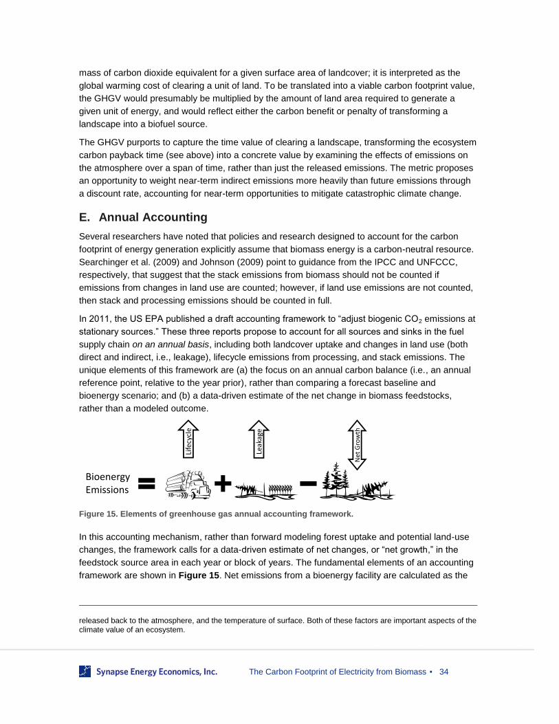
The Carbon Footprint of Electricity from Biomass
▪ 34
mass of carbon dioxide equivalent for a given surface area of landcover; it is interpreted as the
global warming cost of clearing a unit of land. To be translated into a viable carbon footprint value,
the GHGV would presumably be multiplied by the amount of land area required to generate a
given unit of energy, and would reflect either the carbon benefit or penalty of transforming a
landscape into a biofuel source.
The GHGV purports to capture the time value of clearing a landscape, transforming the ecosystem
carbon payback time (see above) into a concrete value by examining the effects of emissions on
the atmosphere over a span of time, rather than just the released emissions. The metric proposes
an opportunity to weight near-term indirect emissions more heavily than future emissions through
a discount rate, accounting for near-term opportunities to mitigate catastrophic climate change.
E. Annual Accounting
Several researchers have noted that policies and research designed to account for the carbon
footprint of energy generation explicitly assume that biomass energy is a carbon-neutral resource.
Searchinger et al. (2009) and Johnson (2009) point to guidance from the IPCC and UNFCCC,
respectively, that suggest that the stack emissions from biomass should not be counted if
emissions from changes in land use are counted; however, if land use emissions are not counted,
then stack and processing emissions should be counted in full.
In 2011, the US EPA published a draft accounting framework to “adjust biogenic CO2 emissions at
stationary sources.” These three reports propose to account for all sources and sinks in the fuel
supply chain on an annual basis, including both landcover uptake and changes in land use (both
direct and indirect, i.e., leakage), lifecycle emissions from processing, and stack emissions. The
unique elements of this framework are (a) the focus on an annual carbon balance (i.e., an annual
reference point, relative to the year prior), rather than comparing a forecast baseline and
bioenergy scenario; and (b) a data-driven estimate of the net change in biomass feedstocks,
rather than a modeled outcome.
Figure 15. Elements of greenhouse gas annual accounting framework.
In this accounting mechanism, rather than forward modeling forest uptake and potential land-use
changes, the framework calls for a data-driven estimate of net changes, or “net growth,” in the
feedstock source area in each year or block of years. The fundamental elements of an accounting
framework are shown in Figure 15. Net emissions from a bioenergy facility are calculated as the
released back to the atmosphere, and the temperature of surface. Both of these factors are important aspects of the climate value of an ecosystem.
Leak
age
Life
cycl
e
Net
Gro
wth
BioenergyEmissions

The Carbon Footprint of Electricity from Biomass
▪ 35
sum of life cycle emissions (transport, losses, and avoided decomposition if applicable) and
induced leakage outside of the system, minus the net growth of the system.34
By combining uptake and direct land use change into a single parameter of net growth, the
mechanism can recognize carbon-managed landscapes (no net change or increasing stocks)
versus areas in which land-use change has decreased standing biomass. Therefore, if an area is
able to maintain a carbon-balanced ecosystem, there is no land use penalty; however, if carbon
stocks falls over time, this decline would be counted against a bioenergy facility.
Theoretically, should it be desirable (from a GHG perspective) to implement wide-scale bioenergy
that might require land use conversions (e.g., changes from forestry to bioenergy crops),
bioenergy facilities might incur significant penalties in near-term years as new land-use patterns
are established, and, after a new equilibrium is reached, begin netting net zero (or close to net
zero) emissions where land use change is no longer a question.
Policies that have adopted an annual or line-item accounting framework
United Nations Framework Convention on Climate Change (2006 IPCC Guidelines): Under
the United Nations Framework Convention on Climate Change, carbon emissions from biomass
combustion for electricity are accounted for not in the Energy sector (where they are reported as
zero), but in the Agriculture, Forestry, and Other Land Use (AFOLU) sector.
Kyoto Protocol (1998): The Kyoto Protocol caps energy emissions for participating countries but
does not regulate land use changes in developing countries. The Kyoto Protocol references the
1996 IPCC guidelines for calculating greenhouse gas inventories, which state that: “[w]ithin the
energy module biomass consumption is assumed to equal its regrowth. Any departures from this
hypothesis are counted within the Land Use Change and Forestry module.” However, the Kyoto
Protocol only requires accounting for land use changes from afforestation/reforestation and
deforestation activities (Article 3, paragraph 3), and only in industrialized (Annex I) countries, so
leakage and other land-based emissions are not accounted for under the Kyoto Protocol.
The Clean Development Mechanism (CDM) of the Kyoto Protocol allows Annex I countries to
develop emission reduction projects in non-Annex I countries (developing countries) and to credit
those reductions toward their own reduction obligations (or sell the credits). CDM uses the 2006
IPCC methodology to account for project emissions but includes only afforestation and
reforestation (A/R) projects. The CDM limits the kind of biomass that can earn credits to
“renewable biomass,” defined as:
woody or non-woody biomass originating from land areas that are forests, croplands,
and/or grasslands, and either remain in their present state or (in the case of crop- and
grasslands) are reverted back to forests; are sustainably managed for the preservation of
34
It should be noted that the EPA (2011) framework includes more factors than are represented in this distilled version, and includes an in depth discussion of the factors and how to calculate or estimate their values. However, it
should also be noted that the EPA framework includes, for the purposes of calculating “net biogenic emissions,” stack emissions (or “potential gross emissions”). It is our understanding that including stack emissions in this calculation would double count biogenic emissions, and thus we have excluded this factor above. The EPA
framework and its implications (and potential correction) are discussed in more depth in the “Implications” section below.

The Carbon Footprint of Electricity from Biomass
▪ 36
overall carbon stocks; and comply with any national or regional forestry, agricultural, and
nature conservation regulations
biomass residue, the use of which will not decrease the carbon pools from which the
residues are drawn
the non-fossil fraction of an industrial or municipal waste stream.
The CDM also disallows the use of pools that can be demonstrated to have carbon stocks that are
increasing faster or decreasing more slowly with the project than without it. The baseline for a
CDM project is what would have occurred without project funding.

The Carbon Footprint of Electricity from Biomass
▪ 37
5. Implications
The accounting frameworks presented above span a range from highly simplified working
assumptions to model or data-driven estimates of current or potential emissions (or avoided
emissions), and include a very wide range of assumptions about what should be included or
excluded, over what timeframe, under what conditions, and across what scale. The following
section represents our analysis of the implications of these various accounting frameworks applied
in a regulatory or policy setting, and questions, concerns, and adjustments.
A. Implicit or explicit carbon neutrality
If biomass is obtained from a carbon-managed ecosystem35
in which real sequestration
opportunities are not forgone,36
and emissions from harvesting, transporting and processing the
biomass are equal to the avoided emissions of not doing so,37
and if this biomass resource were
not previously in use for either product or energy, and if using this biomass does not change the
demand for products previously obtained from the carbon-managed ecosystem,38
then it is
feasible that this biomass resource, combusted as bioenergy, is indeed carbon neutral. However,
the circumstances in which all of these criteria are met are difficult to achieve and only apply to a
limited range of biomass feedstocks. These might include some forestry litter and thinning slash
(the amount of which may vary depending on the source), non-marketable or combusted forestry
wastes, non-utilized agricultural residuals, and other waste products.
However, declaring all biomass carbon neutral by definition sets the stage for a massively
perverse incentive under any form of carbon regulation or legislation, and could cause large
market distortions for both local and international feedstocks.
For example, if there is no mechanism to either prevent or account for land converted from high
carbon storage to low carbon storage (i.e., the “New Production” or “Intensified Production”
scenarios), and carbon prices are high enough to move new forests into production, an
assumption of carbon neutrality could result in large-scale shifts of carbon from sequestered
biomass stocks to the atmosphere.
Similarly, with an assumption of carbon neutrality, a carbon price could drive other biomass
products into bioenergy, rather than other uses, triggering leakage and undermining any potential
carbon benefit in bioenergy (see “Diverted Production” scenario).
New Production Risk
What are the global carbon implications of assumed carbon neutrality? Melillo et al. (2009) explore
two scenarios in which biofuels are used as a prominent mechanism to meet limits imposed on
industrial and fossil fuel GHGs. In a “deforestation” scenario, where existing natural ecosystems
35
“Carbon-managed ecosystem” an ecosystem in which carbon stored in standing biomass, litter, and soils does
not decrease over time (not including seasonal variation). 36
“…real sequestration opportunities are not forgone..” i.e. a managed forest does not replace a growing forest that, but for bioenergy would have continued growing and sequestering new carbon 37
“…not doing so” e.g. if litter is landfilled, and combusting the litter avoids methane emissions 38
“…change demand for products…” i.e. leakage

The Carbon Footprint of Electricity from Biomass
▪ 38
can be cleared for biofuel production, managed landscapes grow 40% larger than today (or by 17
million km2), the vast majority of which are dedicated to biofuels (85%). This scenario results in a
loss of about 21 petagrams of carbon (PgC) by 2050 (relative to 2020) from biofuel land use
conversion alone—equivalent to about 86 billion short tons of CO2 committed to the atmosphere—
or up to 103 PgC including indirect effects and conversions (>400 BtCO2). In the best case, with
no indirect effects and full fossil substitution, the carbon debt lasts through the mid-century with a
net increase of about 5-10 PgC until 2045.
Diverted Production Risk
On a smaller and more local scale, we can examine the impacts of a carbon price on the biomass
supply chain for a particular generator under a carbon-neutral assumption. The Schiller 5
generating station in New Hampshire is a 50 MW steam boiler. In 2006, the unit was converted
from coal-fire to wood and was re-branded the “Northern Wood Power Project” (the official name
remains unchanged). According to a recent docket (NH PUC DE 10-195, January 2011 G.A.
Long), the unit pays approximately $27/ton of wood (presumed delivered, dry). What sort of
carbon price might be required to start diverting paper pulpwood into this generator? The U.S.
Billion Ton Update (US DOE, 2011) shows an estimated supply curve for pulpwood, starting at
around $60/ton (Figure 16).
Figure 16. National supply curve for pulpwood. US DOE Billion Ton Update (2011)
In order to start displacing pulpwood to the bioenergy market, suppliers would have to have a
sufficient price signal to start selling wood to biomass energy facilities instead of paper producers.
If other (higher efficiency) units were also purchasing wood at the same price, we estimate that it
would take a carbon price of approximately $26/tCO2 to start diverting pulpwood to generators.39
39
Assumed energy content of wood of 13 MMBtu/ton (20% moisture), plant heat rate of 10 MMBtu/MWh, yielding a
“recoverable power content” of about 1.3MWh/ton of wood (at which the current fuel price would be $21/MWh). To reach $60/ton, divide the price difference ($60-$27=$33/ton) by the recoverable power content (1.3MWh/ton) to

The Carbon Footprint of Electricity from Biomass
▪ 39
This price differential represents the premium that could be commanded by biomass energy
generators for “not emitting carbon” under an assumption of carbon neutrality (i.e., generators
could purchase high-cost fuel, sell carbon credits, and still break even). The generators would
therefore be willing to pay the $60/t wood price, and pulpwood sellers would begin diverting from
the paper market. The supply curve above would saturate at about $60/tCO2 with all identified
pulpwood diverted to bioenergy.
With pulpwood diverted to bioenergy, paper and particle board producers might start looking to
other sources of pulpwood, either outside the country or from new production lands. This would
lead to either new production or leakage, undermining the CO2 benefit of the bioenergy.
Other agencies have recognized this risk, even if not explicitly stated. For example, in discussing
short rotation woody crops (SRWC), the BRDB (2008) suggests that “SRWC typically face strong
price competition from the pulp/paper industry, which faces a shortage of supply from traditional
sources of pulp logs” and that “most SRWC are currently harvested for uses other than bioenergy
as the economics of SRWC biomass are not yet favorable compared to alternative uses such as in
the pulp and paper industry.”
The BRDB (2008) review suggests that policy incentives could tip the balance between what is
used as a bioenergy feedstock versus what is available for other productive use:
Future changes in relative prices, either as a result of new policy initiatives
(mandates, taxes, subsidies) or market forces can either improve or worsen
the competitiveness of biomass as feedstock. If the relative prices of a
substitute energy feedstock (coal) rise, due to either taxes or market forces,
biomass will become more competitive in the bioenergy energy market.
Likewise, a decline in the relative price of pulp due to market forces would
improve the competitive position of biomass vis-a-vis pulpwood and allow
biomass to be drawn into energy production rather than as feedstock for
industrial wood products.
The US DOE Billion Ton Update (US DOE, 2011) notes the same potential tradeoff:
As the price for wood fuel feedstock approaches the price for pulpwood in a
locality, there will be additional acres harvested for pulpwood to be used for
energy, and some of the pulpwood going to pulp or panel mills will be diverted
to wood energy use.”
Similarly, the IPCC (2011) cautions:
For policymakers wishing to support the development and deployment of RE
technologies for climate change mitigation goals, it is critical to consider the
reach $26/MWh. This price represents the opportunity cost of not burning biomass at other coal units. Since those coal units have an emissions rate of about 1tCO2/MWh, the effective CO2 price to switch to pulpwood biomass
would be about $26/MWh for fairly efficient coal units. At Schiller 5’s heat rate (13.68 MMBtu/MWh, EIA Form 923 2010), the carbon price would have to be closer to $35/tCO2.

The Carbon Footprint of Electricity from Biomass
▪ 40
potential of RE to reduce emissions from a lifecycle perspective, an issue that
each technology chapter addresses. For example, while the use of biofuels
can offset GHG emissions from fossil fuels, direct and indirect land use
changes must be also be evaluated in order to determine net benefits. In
some cases, this may even result in increased GHG emissions, potentially
overwhelming the gains from CO2 absorption.”
Implications of Carbon Neutrality in Policy
The US DOE’s Energy Information Administration (EIA) runs a comprehensive Annual Energy
Outlook (AEO) model for US energy supply and demand, which is informative in this case for
examining the implications of a proxy “carbon neutral” assumption. The AEO product has typically
assumed that biomass power (municipal solid waste, co-fire, and dedicated facilities) are carbon
neutral, and does not include these facilities in carbon pricing schemes, unless otherwise
requested and specified. In November 2011, the EIA ran a model variant by request of Senator
Bingaman testing a policy scenario with a “Clean Energy Standard” (CES), wherein all generation
from renewable energy sources (including all biomass and co-fire sources) earn full CES credit,
and new hydroelectric and nuclear facilities also earn the credit. New and existing fossil facilities
earn partial credits based largely on their carbon dioxide emissions rate (see US DOE, 2011
Bingaman Study). Starting in 2015, the CES requirement rises over time, creating demand for
renewable energy and low-emissions technologies.
From a biomass/carbon perspective, this model is an important test case: CES credits are
approximately inversely proportional to CO2 emissions rates and thus the rising CES requirement
simulates a gradually tightening CO2 cap. However, this CES assumption assigns full credit (i.e.,
carbon neutrality) for biomass generation. The results of the reference case model and the CES
model are shown in Figure 17 for new renewable energy obtained after 2014.
Figure 17. New renewable energy generation (TWh) produced under the AEO 2011 reference case
(left) and the Bingaman Clean Energy Standard (CES) through 2035.
The most notable component of these graphs shows that biomass co-fire makes up a very large
fraction of new renewable generation through about 2022, at which point presumably the price of
CES credits makes wind increasingly attractive. The biomass facilities in this assessment are, by
far, the largest segment of new renewable energy under the assumption that these facilities
0
50
100
150
200
250
300
350
400
New
Ren
ewab
le G
ener
atio
n (
TWh
)
Annual Energy Outlook 2011 (Reference Case)New Renewable Generation (delta to 2014)
Offshore Wind
Wind
Solar Photovoltaic
Solar Thermal
Biomass Cofire
Dedicated Biomass
Biogenic Municipal Waste
Geothermal
Conventional Hydropower0
50
100
150
200
250
300
350
400
New
Ren
ewab
le G
ener
atio
n (
TWh
)
Annual Energy Outlook 2011 (Clean Energy Standard Case)New Renewable Generation (delta to 2014)
Offshore Wind
Wind
Solar Photovoltaic
Solar Thermal
Biomass Cofire
Dedicated Biomass
Biogenic Municipal Waste
Geothermal
Conventional Hydropower
The Carbon Footprint of Electricity from Biomass
▪ 41
warrant full CES credit, or are effectively carbon neutral, rising to 166 TWh of co-fire generation by
2022.
Referring to the earlier Schiller example and using an estimated recoverable power rate of 1.3
MWh/ton of wood, we might estimate that this scenario in the AEO requires 129 million dry tons
per annum, which, according to the US DOE Billion Ton Update (2011) might be supplied by a
combination of (from the least impact resource, upwards): sustainably harvestable logging
residues and thinning biomass (about 77 million try tons),40
divertible pulpwood (about 39 million
dry tons)41
, and agricultural crop residues available for less than $50/ton (about 130 million dry
tons).42
While the EIA analysis of the Bingaman policy shows a substantial expansion of biomass energy,
this is not a certainty, and other analyses have shown wind, solar, and geothermal to play a larger
role than biomass43
. Nevertheless, appropriate rules for accounting for the emissions associated
with biomass should be in place at the onset of any such policy. In a paper examining co-fire
potential in the Southeast, Abt et al. (2010) found that when about 60 million green tons (~30
million dry tons) of biomass were required in 2021, it was economic to obtain about half of the
biomass from some form of residual, while the remainder was either diverted from pulpwood or
produced from new forests or intensified harvests. This study represented less than a quarter of
the potential under consideration in the AEO scenario.
Similarly, Sedjo and Sohngen (2009), referring to a cellulosic ethanol liquid-fuels policy, suggest
that increasing demand for biomass for energy could raise wood prices by 20%,44
diverting
conventional wood products and driving wood production overseas.45
Overall, it is our judgment that the risk of market distortions and unintended consequences from
the a priori assumption of carbon neutrality are unacceptable from a carbon accounting
standpoint. There is no guarantee that all biomass would be obtained from feedstock that do not
result in net emissions; embedding this assumption in the emissions of bioenergy is likely to result
in higher emissions to the atmosphere than would be expected by simply counting biomass as
carbon neutral.
A set of “second best” policies could mitigate some of the risks of a carbon-neutral assumption;
such policies might limit biomass feedstocks to those that come from already managed lands and
do not displace other valuable wood products, demand sustainable forestry practices, limit the
amounts of residue products collected, and require high-efficiency end uses of biomass. These
are all valuable best principles, but in the end a methodology for proper accounting of the land use
40
Billion Ton Update (2011), Text box 3.4 41
Billion Ton Update (2011), p46 and Figure 3.17 42
Billion Ton Update (2011), p68 43
See, for example, an NREL analyses “Impacts of an 80% Clean Energy Standard on the Electricity Generation Sector “ available at: http://www.rff.org/Documents/Events/Seminars/110727_CES/110727_Steinberg.pdf 44
“The projections show biofuel use increases wood consumption by about 60 percent by the early 2020s. In the short run, the price run‐ups in the United States would most likely be greater. The higher prices choke off some of the increased consumption of wood for conventional uses that would have occurred.” 45
“In the base case, the model projects movement from net exports of about $250 million in 2010 to a wood trade deficit (net import) of about $1.2 billion by 2050.”

The Carbon Footprint of Electricity from Biomass
▪ 42
implications of biomass production must be developed simultaneously with any policy that would
promote the large-scale use of biomass.
B. Life Cycle Analysis
Unto itself, life cycle analysis (LCA) is an established concept, used to compare and contrast the
environmental impacts of products, services, and policies. In the context of biomass energy,
however, it is our assessment that the concept has been applied inconsistently, and occasionally
with assumptions that give undue favor to bioenergy. In particular, while there is no particular
reason that such a pattern should have emerged, and it is certainly not universal in the field, there
are a few prominent trade papers touted as “state of the art” life cycle analyses that appear to
strongly support bioenergy (i.e Lippke et al., 2011; Bowyer et al., 2011; Malmsheimer et al., 2011;
Perez-Garcia et al, 2005).
There are two concerns that we find with current life cycle emissions frameworks:
Inconsistent system boundaries or basis assumptions
Life cycle analyses are clearly the correct mechanism for exploring the emissions implications of
harvesting, transporting, and processing biomass for energy products; the procurement and use of
the fuel product and all of the ramifications thereof are well-suited to the LCA community.
However, it is not always clear under what circumstances an LCA includes relativistic terms (i.e.,
avoided emissions from non-landfilled waste) or to what extent indirect impacts are considered or
not. This concern extends both to questions of land use (if land use changes are considered at all)
and avoided emissions (often embedded in the footprint value itself). Underlying assumptions are
critical: including or excluding various aspects of an LCA drive particular conclusions.
For example, Davis et al. (2009) show a wide range of life cycle carbon benefits for biomass
energy across studies, 46
and explain that “inconsistencies in the assumptions applied to biofuel
LCA [life cycle assessments] lead to variable and, in some cases, conflicting results about their
GHG and energy mitigation potential.”
Similarly, Rabl et al. (2007) note that “in a part of the LCA community, a special convention has
been established according to which CO2 emissions need not be counted if emitted by biomass….
to avoid [absurd] conclusions, we recommend that emission and removal of CO2 be counted
explicitly at each stage of the lifecycle.”
The difference between a positive or negative outcome in life cycle assessment may rest on the
choice to characterize land use changes and leakage (Liska and Cassman, 2008), the assumption
that a biomass energy resource will displace specific fossil alternatives (i.e. Lippke et al., 2011), or
assumptions about the alternative fate of biomass not used for energy (i.e. Mann and Spath, 2001;
Heller et al., 2004).
46
The study shows that the greenhouse gas “displacement” of switchgrass as a liquid biofuel varies between -114% (the fuel is 14% better than carbon neutral) to 50% (the fuel produces 50% more carbon than its direct
emissions), depending on the author and study assumptions. The later of these studies included emissions from direct and indirect land-use changes, while the later did not, and included indirect nitrous oxide emissions.

The Carbon Footprint of Electricity from Biomass
▪ 43
We stipulate that while there may not be an absolute correct mechanism for defining system
boundaries (particularly in such long-lived and global phenomena as trade in biomass products
and the extended impacts of greenhouse gases), there are minimum criteria that should and can
be met if biomass energy products are to be correctly assessed on a level playing field with other
energy options.
Inconsistent framework with other energy sources
There are two reasonable purposes to create an internally consistent framework for carbon
accounting in biomass: (a) to assess long-term resource potentials in an atmospherically
meaningful fashion, and (b) to inform energy planning at anywhere from the policy to utility scale.
Currently, life cycle emissions are not part of the standard calculus for policy or utility-scale
planning—it is not standard practice to estimate the emissions from uranium processing, solar
array manufacture, natural gas extraction, or coal mining and transport. While it may prove
valuable to incorporate such life cycle costs into formal planning, at the moment, biomass energy
should probably remain internally consistent with other energy sources, where extraction,
transport, and processing emissions are typically not estimated.
C. Greenhouse Gas Value
The model framework for the Greenhouse Gas Value (GHGV), while supposing to put the impacts
from biomass energy emissions on a level playing field, requires a very complex set of
formulations and assumptions to be implemented, including:
A model of vegetation dynamics of the pre-existing landscape, and its contribution to
carbon (and other greenhouse gases) emissions or sequestration, as well as biophysical
characteristics (albedo and evapotranspiration), and the rate at which that landscape
might reasonably be expected to be disturbed by natural processes (e.g., fire and
windstorms);
An explicit choice of an analytical timeframe (on the order of a century to multiple
centuries), an ecosystem timeframe (on the order of decades),47
and an annual discount
rate, if desired, to account for the opportunity cost of avoiding catastrophic climate
change. Each of these factors can be chosen by an analyst—but each dramatically
impacts the value of GHGV. Moreover, each value may legitimately be different for
different ecosystems, implying that this method may be difficult to standardize across
multiple practices.
The GHGV module, aside from the complexity of implementation, presents other difficulties as a
regulatory tool as well: by giving either credit or penalty to future emissions or sequestration, the
system presupposes how land cover might evolve in the future. As presented, the GHGV
mechanism does not appear to have the flexibility to accommodate practices such as intensified
harvests on existing land cover, and offers no mechanism to account for spatial leakage.
47
The ecosystem time frame is described as “the number of years over which the ecosystem is presumed to affect the atmosphere.”

The Carbon Footprint of Electricity from Biomass
▪ 44
D. Temporal Lag Estimation
Some researchers have suggested that the temporal lag problem can be solved using a discount
rate (Anderson-Teixeira and DeLucia, 2011) to account for the risk of catastrophic climate change,
while others use the length of time in a lag as an independent assessment of whether a project
has a GHG benefit (Manomet, 2010). Others intrinsically discount the lag concern as irrelevant to
long-term climate change forcing, and cite the long-run benefit of a biomass energy economy
(Sedjo, 2011).48
Finally, others suggest that investing today in biomass by planting future energy
crops may solve the temporal lag conundrum (Marland, 2010); the temporal lag problem is not
solved, however, if biomass is harvested elsewhere today with only the understanding that it will
be replaced by plantings in the future.
From our standpoint, the temporal lag accounting schema is problematic for several reasons:
a) Risks simply kicking the can down the road: relying on future behavior does not
ensure regulatory accountability. In other words, circumstances may change dramatically
from the time a policy is envisioned, rendering it difficult or impossible to follow through on
a promise to sequester carbon.
b) No market signal: Does not provide a mechanism to send current biomass suppliers or
bioenergy producers a market signal for how biomass feedstocks should be obtained;
c) Relies heavily on long-term models of biomass growth, mortality, and use: while
managed growth models are well calibrated, natural ecosystem dynamics models
(including disturbances) require significant data and observations;
d) Relies on long-term displaced emissions assumptions: the concept that eventually a
debt will be re-paid by offsetting higher emissions technologies relies on the assumption
that high emissions technologies will remain in use in the base case, even as policy (e.g.,
stringent EPA regulations) and technology (e.g., dropping prices for wind and solar
technology) begin to change the market even in the absence of renewable or carbon
policies;
e) Moves the target: if the risk of a climate tipping point can be mitigated by implementing
low carbon activities today (UNEP, 2009), then accepting a pulse of emissions today for
climate benefits perhaps decades away may be inappropriate from a climate protection
standpoint. While it may ultimately be acceptable to accept higher emissions today in
return for low emissions in several decades (i.e. a 30-50 year payback), such a tradeoff is
highly dependent on climate modeling and poses a risk that should not be undertaken
lightly (BERC, 2012).
48
From Sedjo (2011): “Even if policymakers look for short-run approaches, long-term sustainable solutions will undoubtedly be required. The contest is a marathon, not a sprint. Lowering carbon emissions from energy
production by 2020, in itself, does not address the fundamental problem of reducing net emissions over the centuries.”

The Carbon Footprint of Electricity from Biomass
▪ 45
6. Annual Accounting: A Feasible Regulatory Mechanism
The annual accounting framework solves some of the difficulties posed in the temporal lag
framework by (a) substituting observed data for long-term models and (b) assigning credit or
emissions to processes that occur today, thereby incentivizing carbon-beneficial behaviors. As
described earlier, if a determination was made that near-term land use emissions were acceptable
for long-term gains, this framework would not inhibit this policy decision, but would correctly track
emission sources and sinks at the time the carbon is committed to the atmosphere.
As one example of an annual framework implemented in a simulation model, Abt et al. (2010)
produced a paper examining the greenhouse gas implications of a theoretical mandatory RPS
requiring 10% co-fire in southeastern US states. The results of this paper are useful for illustrating
intensified production, leakage, and residual harvesting scenarios in tandem. These researchers
did not a priori assume carbon neutrality, but created a scenario in which biomass must be
procured for co-fire. The paper examines regionally competitive wood, pulp, and residual markets
and is based on long-term forestry models calibrated to current-day observations. The paper
explores two different scenarios, in which 25% or 50% of forestry residuals are gathered for co-fire
in regional coal plants. In the more residual intensive scenario (i.e., more of the required biomass
can be served through forestry residuals), just over half (53%) of wood is derived from residuals,
while the remainder is from either diverted pulpwood (31%) or intensified production (16%). When
fewer residuals can be obtained from the forest, the remainder is procured from either new
production, intensified harvests, or diverted pulpwood.
The Abt (id) paper examines carbon implications by charting annual emissions from direct land
use change against displaced emissions from coal co-fire, and concludes that the avoided
emissions exceed land use emissions. However, if we exclude displaced emissions from the
assessment of carbon impact (see the Primer under Displaced Emissions), the land use change
impact is substantial. Between the two scenarios, in 2026 and beyond, the land use change
results in emissions of about 25-40 million tCO2 for about 50 million MWh of energy yield. We can
suppose that the emissions rate from this system would be about 0.5-0.8tCO2/MWh, or slightly
higher than a natural gas fired generator (0.4-0.6tCO2/MWh) but less than coal fired generation
(~1.0-1.2tCO2/MWh).
A. The EPA Proposed Annual Framework
In 2011, the EPA proposed an annual accounting framework that offers a mechanism to track
emissions from stacks, land use change, losses, and leakage, and adjustments for facilities that
produce long-lived co-products. The innovative component of this mechanism is that it explicitly
tracks carbon stock changes in a particular source region from forestry data and assigns changes
in stock to bioenergy producers that draw feedstock from that source region.
The EPA research paper, however, illustrates the difficulties inherent in choosing a source region.
The paper states that “the spatial scale of accounting must be large enough that accurate data are
available, but small enough to capture important regional characteristics such as growth rates and
variation in market demand for feedstocks.” In the first case example, the paper explores how the
estimate of net emissions from a biomass facility changes if the “source area” is a single state,

The Carbon Footprint of Electricity from Biomass
▪ 46
versus if the source area is a larger region—in this case, both regions where net background
biomass is increasing.
…where a feedstock is sourced from a small landscape that currently has an
increasing stock of carbon, but the proposed new facility demand would
create declining carbon stocks, the proposed plant will have greater than zero
NBE [net biogenic emissions]… However, in this same case, if accounting is
done at the larger regional landscape level,… the feedstock-derived
emissions are assumed to be fully removed from the atmosphere via forest
growth.
In both of these cases, the generator is effectively held responsible (or granted credit for) changes
in land use that may be well outside of its area of influence. Using an extreme example, assume
that the biomass generator has sourced all biomass from ideal, sustainable sources in a region,
and yet other land use practices in the area have caused massive declines in regional biomass in
all areas except those held by the generator. In this framework, the generator is penalized for
others’ actions. At the other end of the spectrum, a generator using an inappropriate supply chain
in an area undergoing natural sequestration would reap a reward for others’ actions (and inaction)
as well.
The EPA paper suggests that this problem might be alleviated by defining “working” lands from
which feedstock is actively procured and “reserved” lands that are inaccessible to biomass energy,
such as parks, easements with specific prohibitions, and possibly small landholdings (see
Buchholz et al., 2011). Restricting the analysis to working lands could (a) ensure that changes in
the biomass carbon stock are largely attributable to management decisions rather than other
phenomena such as municipal growth or natural disturbances, and (b) reduce “free ridership” from
biomass energy producers when non-managed landscapes gain carbon, but managed landscapes
lose carbon stocks.
Ultimately, the annual accounting methodology results in an estimate of the tons of land use
emissions, if any, attributable to any generator (or cohort of generators) on an annual basis, and
thus could be used for both carbon regulation (wherein there is a cost to emitting carbon dioxide)
and effective energy planning. The mechanism is transparent, generalizable, and internally
consistent. We have critiqued the equation set proposed by the EPA; this critique is found in

The Carbon Footprint of Electricity from Biomass
▪ 47
Appendix C: Comments on EPA Annual Accounting Framework.
Distinguish “good” and “bad” actors
It is feasible that under deeper bioenergy penetrations, there may be “good” and “bad” actors who
either ensure that they work with low carbon feedstock (such as wastes and residuals) or do not
choose to work with low carbon feedstock (such as whole tree use or pulpwood diversions). In
these cases, it would be unfair to pool these users in the same land-use categories. Instead,
“good actors” should have the opportunity to show that they have not contributed to biomass
carbon losses.
Environmental Defense Fund (EDF) has proposed a mechanism by which if a generator chose to
document their supply chain from only residuals and wastes, that generator, having presented the
burden of proof, could opt out of the calculation. Any changes in the biomass carbon stock would
be allocated to generators that had not demonstrated a neutral supply chain (see Hamburg et al.,
2011).
The natural incentive is that generators operating in regions in which there might be a loss of
carbon from standing biomass would be incentivized to demonstrate that their feedstock is carbon-
neutral. This would discourage new entrants into areas where unsustainable practice already
occurs, and provide an additional incentive for generators to secure a reasonable supply chain if
their region is at risk of a carbon loss.
B. A Consistent Framework
Using an internally and externally consistent framework for counting emissions from bioenergy will
be critical for both system planning and policy. There are significant risks in defining, a priori, the
emissions benefits (or impacts) of bioenergy; but a consistent framework will allow regulators and
policymakers to determine how large of a role biomass energy should play in a growing renewable
energy market. The IPCC notes that, under a consistent framework, it may be reasonable to
pursue significant bioenergy penetration, but that such a pathway entails risk:
From a strict climate and cost efficiency perspective, in some places a certain
level of upfront LUC emissions may be acceptable in converting forest to
highly productive bioenergy plantations due to the climate benefits of
subsequent continued biofuel production and fossil fuel displacement. The
balance between bioenergy expansion benefits and LUC impacts on
biodiversity, water and soil conservation is delicate. Climate change mitigation
is just one of many rationales for ecosystem protection.(IPCC, 2011)
While precaution does potentially slow the development of bioenergy, such precaution may be
warranted. A consistent carbon accounting framework would be independent of sustainable
forestry practices, but such practices may be tremendously important for good carbon outcomes
from bioenergy use. Proceeding with a clear understanding of the carbon costs and risks of
bioenergy will be fundamental if the resource is to be used as a serious mitigation technology.

The Carbon Footprint of Electricity from Biomass
▪ 48
C. The Value of a Precautionary Approach
Mounting a detailed and site-specific accounting framework for estimating the greenhouse gas
implications of biomass energy is an additional burden for generators not currently faced by other
generators, particularly within the renewable energy community. This burden will make it more
difficult for new facilities to enter the field, and potentially discourage resource development in the
short term. However, in our opinion, such a precautionary approach is deeply warranted, provides
direct, financial accountability back to generators, and creates a transparent, auditable mechanism
for both internal and external parties to determine the carbon implications of biomass generation.
Such a mechanism is absolutely fundamental if biomass generators are to be given credit for
avoiding emissions of carbon dioxide, and avoids perverse incentives for combusting biomass in
otherwise productive use, or unintended consequences of reducing standing biomass either
locally or through indirect land use change.
Existing biomass generation has not traditionally targeted the types of feedstock that are of
concern in this paper (e.g., energy crops, new forestry management, or intensified management
practices), yet recent proposals and the economics suggest that the day is not far afield when
generators will start diverting paper and pulp production, or start replacing forests or agricultural
lands with short-rotation woody biomass crops. At such time that these substitutions begin
occurring, the biomass electricity sector will have overstepped any reasonable definition of carbon
neutrality. It is our opinion that a policy with the implicit or explicit goal of reducing electricity sector
emissions through the use of biomass must urgently put in place an accounting framework such
that all players in the market are subject to fair and transparent rules. This accounting framework
should not be unduly restrictive so as to restrict small or innovative generators from participating,
but must address the potential for land use change emissions that might otherwise undermine the
goals of the policy. Again, if it is determined that there is a dramatic atmospheric benefit to be
gained, even through massive land-use conversion for biomass energy, the proposed accounting
framework would allow for such a tradeoff, but maintain a clear understanding of the fate of
biomass carbon.
Proponents have also argued that implementing a biomass energy economy effectively replaces
fossil fuels, particularly where co-fire operations can directly displace coal. It should be noted that
some within the coal community may similarly see biomass co-fire as an opportunity to invest new
capital in aging infrastructure, avoid environmental penalties (such as SO2 requirements), and
promote these facilities as “clean”—effectively extending the life of coal infrastructure that might
otherwise retire (see Eisenstat et al., 2009). If GHG reductions are more effectively realized
through the retirement of coal infrastructure, then extending the life of older facilities through
marginal biomass co-fire (5-15%) could be considered largely counterproductive.
We conclude that there is room in the electricity generation sector for biomass energy as a
greenhouse gas mitigation tool. However, to effectively reduce GHG emissions, biomass facilities
should be subject to a clear and rigorous accounting framework that results in estimates of GHG
emissions consistent with other energy resources. The incentives offered to biomass generation, if
targeted towards GHG reductions (implicitly or explicitly) should be indexed to the outcome of this
accounting mechanism.

The Carbon Footprint of Electricity from Biomass
▪ 49
7. Appendix A: Bioenergy Carbon Neutrality in Current Framework and Policies
This appendix presents descriptions of, and/or excerpts from, gray literature, academic literature,
and policy frameworks that either explicitly or implicitly assume that bioenergy is a carbon-neutral
energy resource.
Morris (2008)
Biomass and biogas energy systems are generally recognized to be carbon
neutral, because the carbon in the fuel is already part of the global stock of
carbon that circulates between the atmosphere and the biosphere. As carbon-
neutral energy sources, bioenergy generators will not have to acquire
greenhouse-gas emissions allowances to offset their stack emissions of CO2.
… The benefits of reducing the warming potential of net biogenic greenhouse-
gas emissions associated with biomass and biogas energy generation are not
a part of the REC, and should be convertible into greenhouse-gas offsets that
bioenergy generators can market in addition to their electricity and REC
products.
Eisenstat et al. (2009)
The main reason to use cofiring, of course, is environmental: Sustainably
grown biomass is widely recognized as a greenhouse gas-neutral fuel.
Although other renewable options, such as wind and solar energy, are
"cleaner," in that they do not require burning any fossil fuels, cofiring directly
reduces the levels of sulfur oxide, nitrogen oxide, and carbon dioxide from
emissions-heavy coal-fired facilities. Accordingly, cofiring should be an
increasingly attractive option in today’s regulatory environment.
Sedjo and Sohngen (2009)
An advantage of any wood energy source is that, within the context of GHG
accounting, wood does not generate net carbon emissions given the
assumption of a closed biological cycle. Wood energy is becoming
increasingly popular in Europe because it is often subsidized directly or
indirectly and users are not required to pay carbon emissions taxes.
Penn State, College of Agricultural Sciences (2010)
Biomass is also essentially “carbon neutral,” which is important when you
consider the growing levels of concern and regulation surrounding the release
of carbon dioxide from fossil fuels.
American Forest and Paper Association (2009)

The Carbon Footprint of Electricity from Biomass
▪ 50
The carbon neutrality of biomass is a longstanding and widely established
principle. Organizations recognizing the carbon neutrality of biomass
emissions include the European Union, US EPA and the UN’s
Intergovernmental Panel on Climate Change (IPCC), as well as recent federal
and state legislation promoting renewable electricity and biofuels.
Johnson et al., (2007)
Biomass fuel is C-neutral because they release recently-fixed CO2, which
does not shift the C-cycle. Biomass may generate the same amount of CO2
as fossil fuels per unit C, but every time a new plant grows it removes that
same CO2 from the atmosphere.
Pacala and Socolow (2004)
It is also possible to replace fossil fuels with fluid fuels produced directly from
plant matter (biomass) that is grown sustainably. In the latter case, the use of
“biofuels” makes no net addition of CO2 to the atmosphere; the biofuels
oxidized for energy deliberately through technology would have decayed
(oxidized) elsewhere anyway (wood on the forest floor, for example). A
sustainable biofuel is one obtained from plants that are replaced by new
plants at the same rate as they are used.
Heller et al. (2004)
Willow biomass is grown specifically for electricity generation and thus willow
production is considered to be within the power generation system boundary.
As a result, electricity generation with willow biomass is nearly GHG neutral.
Robinson et al. (2004)
While biomass burning emits CO2, use of biomass is considered carbon-
neutral in the context of climate change if the fuel is sustainably harvested
because the carbon in biomass is part of the active carbon cycle.
McKendry (2002)
Burning new biomass contributes no new carbon dioxide to the atmosphere,
because replanting harvested biomass ensures that CO2 is absorbed and
returned for a cycle of new growth.
US Department of Energy (2004)
Reduced greenhouse-gas emissions: Sustainably grown biomass is
considered a greenhouse-gas neutral fuel, since it results in no net carbon
dioxide (CO2) in the atmosphere. Using biomass to replace 10% of the coal in

The Carbon Footprint of Electricity from Biomass
▪ 51
an existing boiler will reduce the net greenhouse-gas emissions by
approximately 10% if the biomass resource is grown sustainably.
European Union Emissions Trading Scheme (2003)
The Emissions Trading Scheme, which is the primary climate legislation in the European Union,
caps greenhouse gas emissions from energy and industrial facilities and allows the trading of
emissions. The ETS does not cover emissions from agriculture or land use changes and
specifically provides that “the emission factor for biomass shall be zero.” (ETS, Annex IV)
European Union Renewable Energy Directive (2007)
The Renewable Energy Directive estimates emissions from land use changes using a
methodology based on the IPCC Tier 1 calculation of land carbon stocks, with gains and losses
amortized over a 20 year period. The baseline is the land use as of January 2008 or 20 years
before raw material was obtained, whichever was later, and assumes constant carbon stocks. The
Renewable Energy Directive acknowledges the potential for—but has no methodology for dealing
with—indirect land use changes or leakage, as Zanchi, et al. (2010) explain:
In the current EU system, the negative GHG impact of bioenergy is partially
addressed by the adoption of a sustainability criteria framework that should
ensure sustainable provision and use of biofuels and bioliquids. The
regulations require that biofuels and bioliquids comply with a minimum climate
mitigation performance. Once the bioenergy product is accepted in the
system, it is considered carbon neutral for the purpose of binding targets.
Concerning the use of solid and gaseous biomass sources, the Commission
produced only recommendations to Member States on the development of
national sustainability schemes (COM 2010). Therefore no binding criteria are
approved for biomass at this stage at the EU level. The recommended
sustainability criteria for biomass are the same as those laid down for biofuels
and bioliquids.
Environmental Protection Agency Greenhouse Gas Tailoring Rule
In its final Prevention of Significant Deterioration and Title V Greenhouse Gas Tailoring Rule
(GHG Tailoring Rule), EPA had determined that all new and existing sources of greenhouse
gases, including biogenic CO2 (emissions from biomass combustion), in amounts greater than
75,000 tpy CO2-e were subject to PSD and Title V permitting requirements—which would require
monitoring, reporting, and determination of Best Available Control Technology (BACT) for GHGs;
however, in response to a petition for reconsideration of the rule from the National Association of
Forest Owners, EPA decided to defer the applicability of its tailoring rule to biogenic GHG sources
for three years, and so does not currently have a national accounting mechanism for CO2 from
biomass (other than interim guidance suggesting that burning biomass is, itself, BACT).
Western Climate Initiative Mandatory Reporting Rule (2009)
In the WCI’s mandatory reporting rule, if a state hasn’t made a determination of what is “eligible
biomass” (partially defined as carbon neutral), the default rule allows up to 15,000 metric tons of
CO2-e from biomass combustion to be excluded from the mandatory reporting threshold

The Carbon Footprint of Electricity from Biomass
▪ 52
determination, as long as total emissions from biomass are less than 25,000 metric tons CO2-e. If
a state determines biomass to be carbon neutral, then no emissions from biomass combustion are
counted when determining whether a source must report its emissions (WCI ERMR, 2009).
Western Climate Initiative Cap and Trade Program
Under WCI’s cap and trade program, all emissions from eligible biomass are excluded from having
to carry allowances for their emissions. WCI requires individual jurisdictions to define for
themselves what qualifies as eligible biomass “provided it must be carbon neutral.” (WCI, 2010)
Regional Greenhouse Gas Initiative (RGGI, 2007)
Under RGGI, participating states have agreed to cap GHG emissions from the fossil-fueled energy
sector. The RGGI cap and trade program, therefore, pertains only to emissions generated by that
sector. Yet RGGI considers "sustainably harvested biomass" as carbon neutral when it is
converted into electricity, allowing power producers to exclude those emissions from their GHG
emission reduction obligations (RGGI, 2009). It is up to each individual state to form its own
definition of "sustainably harvested" biomass.

The Carbon Footprint of Electricity from Biomass
▪ 53
8. Appendix B: Displaced Emissions on the Operating and Build Margins
The following definitions and descriptions of displaced emissions are derived from several
sources, including Biewald (2005), Broekhoff (2007), Hausman et al. (2008) and Fisher et al.,
(2011). These resources describe mechanisms by which displaced generation and emissions may
be estimated using both data-driven analyses and simulation models.
Displaced Emissions on the Operating Margin
The displacement of generation and emissions on the operating margin is fundamentally a
function of economic dispatch. Economic dispatch governs how most generating units in an
interconnected electrical system are run: the units with the least expensive operating costs (fuel
and operations) are typically dispatched first, and increasingly expensive units are then dispatched
to meet load requirements, subject to transmission availability. The last unit, or cohort of units,
dispatched to meet load in a particular area are called the marginal unit: the last to come online,
they would also be the first to be taken offline if load is reduced. The operational margin is
therefore the correct mechanism to estimate the impact of a new energy project or load reduction
in the near term, holding all other elements of the grid constant (i.e., unit retirement or new units).
For example, given no expected changes in existing capacity, but with an RPS requirement that
demands a new bioenergy facility, there would be no clear individual plant that is displaced.
Rather, the new bioenergy facility would change the dispatch of units more expensive than it, and
marginal resources would be impacted. In the current economy, natural gas resources are often
on the operating margin, and fairly expensive (variable and operating cost) bioenergy facilities
might only change the dispatch of natural gas resources.
There are numerous factors that affect which power plants operate, are committed to operate, or
are held in reserve at any point in time. These factors can include the offer price or short-run
marginal cost; constraints such as ramp rates, minimum up and down times, and other operating
restrictions; transmission or other dispatch constraints; maintenance schedules; unplanned
outages and/or deratings; and environmental constraints (e.g., emissions prices). System
operation can be extraordinarily complicated, but is generally determined by a set of known
procedures that are, in practice, implemented by system operators who implement the procedures
in real time determining generating unit commitment and dispatch. Similar simulation models can
be used to estimate near-term generation decisions and thus emissions implications. Synapse and
other parties have designed mechanisms to estimate operational margins using recent historical
data on operations emissions collected by the EPA and EIA.
Displaced Emissions on the Build Margin
The effect of a project upon reference case capacity additions to the system can be in terms of
“deferring” additions, “avoiding” additions altogether, specifically replacing capacity, or actually
promoting the extended life of existing capacity that would have otherwise retired. These types of
effects, including deferral/avoidance, replacing capacity, delayed retirement, or even replacement
of other renewable technologies, are important elements of the build margin and the analysis of
displaced emissions over the long-term. These types of decisions are typically made using
economic analyses that span a whole fleet (IRP), or even a whole region or interconnect (WECC;
The Carbon Footprint of Electricity from Biomass
▪ 54
EIPC). The following provide hypothetical examples in which these types of scenarios might occur.
All of these scenarios would still call for modeling or analysis of both baseline and bioenergy case
scenarios.
Deferral/Avoidance: A utility’s lowest cost mechanism to meet growing demand may be
to build new fossil capacity. However, in light of a policy promoting bioenergy (e.g., an
RPS), the utility finds that it can build a bioenergy facility instead, avoiding the requirement
for new fossil capacity. In this case, the capacity that is deferred or avoided by the
bioenergy facility could be a basis for estimating avoided emissions on the build margin.
Replacing Capacity: In the face of more rigorous environmental regulations, the cost of
maintaining an older, less efficient, and/or higher emissions power plant is outweighed by
the benefit of replacing the plant. If a bioenergy facility were to be a cost-effective
replacement, the emissions avoided by retiring the existing unit could be an important
component of the displaced emissions.
Extended Life: In some cases, adding biomass co-fire ability to a plant may allow it to
remain operational (or be permitted in the first place), 49
either under an RPS, because
emissions standards may be different for bioenergy facilities than fossil plants, or because
co-firing allows an existing boiler to meet emissions standards (e.g., for sulfur dioxide;
Mann and Spath, 2011). If in the baseline this plant would have retired, but can now
remain operational with a moderate bioenergy component, the difference between the
baseline retirement and bioenergy “extended life” scenario may now result in increased
emissions with the extended life of the fossil component of the facility.
Displacing Renewable Energy: If bioenergy is allowed to participate in a renewable
portfolio standard (RPS), then it will likely compete with solar, wind, geothermal, and other
renewable technologies to meet the RPS at the lowest cost. However, if, in competing
with these other technologies, bioenergy excludes other low-emissions technologies, then
a reasonable baseline for determining the emissions impact of bioenergy might be an
RPS without bioenergy.
49
In May 2009, the State of Kansas announced a settlement allowing the Sunflower Electric Power Corporation to build the new 895 coal-fired Holcomb power plant on the condition (amongst others) that the utility uses the equivalent of 10% biomass co-fire at the facility (Sunflower Electric Power Corp, 2010). It is not clear if the
“reference case” in this circumstance is the coal plant without this provision or no coal plant at all. If it is the former, the biomass co-fire may be displacing new coal. However, if this agreement would not have occurred without the support of bioenergy, then it might be argued that biomass energy has added new coal power, rather than
displaced it.

The Carbon Footprint of Electricity from Biomass
▪ 55
9. Appendix C: Comments on EPA Annual Accounting Framework
The EPA has accepted and synthesized comments on the framework (EPA, 2011b) including a
wide range of suggested approaches on the correct spatial scale in which to examine landscape
changes (from the “fuel shed” to the national level) and the correct time scale over which to
include life cycle emissions, if at all (ranging from full life cycle to alternative fossil futures), and the
extent to which leakage should be examined. Other parties suggested alternate frameworks (as
described earlier in this paper) including life cycle analyses, carbon neutrality based on an
alternative fossil fuel future, and temporal lag framework. However, the synthesis report does not
describe questions about the actual accounting equation set.
The EPA framework calls for the calculation of a “biogenic accounting factor,” a unitless ratio of
the amount of emissions attributable to a biomass facility divided by “potential gross emissions” (or
emissions of CO2 if biomass were combusted completely). From the standpoint of an accounting
framework that can be used for effective policy and planning, the desirable outcomes are either
total emissions, or a net equivalent emissions rate. Total emissions attributable to biomass
energy, called “net biogenic emissions” (NBE) in the framework, would return such a value, and
divided by energy produced, would yield an equivalent emissions rate that could be used in
energy and policy modeling.
The EPA’s framework for calculating net biogenic emissions (NBE) is, distilled, fairly
straightforward. Assuming a facility structured to produce energy only, we can briefly ignore a
number of life cycle and adjustment factors for on-site emissions unrelated to energy, deductions
for products shipped offsite that are not energy related, and losses of biomass between the field
and facility. A simplified version of the equation looks as follows:
( )
where NBE is the “net biogenic emissions” in tons, PGE is “potential gross emissions” of the
facility if all biomass were fully combusted, LAR is defined as a “level of atmospheric reduction”
but is really just a fraction between 0 and 1 as shown below, and LEAK represents estimated
leakage (i.e., indirect land use impacts caused by the facility). Both PGE and LEAK are given in
tons, and LAR is a ratio.
LAR, again simplified, is fundamentally defined as
where GROW is defined as “annualized growth…on the basis of the annual change in above-
ground live tree biomass.” However, because LAR is defined by PGE, simple algebra allows us to
re-arrange the first equation to become:
Simply stated, this equation states that the total net emissions from a bioenergy facility equal the
stack or tailpipe emissions (PGE) minus the amount of feedstock that has grown in the source
area (GROW) plus the indirect effects attributable to the biomass facility.
In practice, the GROW term would measure actual forest plots on an annual or semi-annual basis
and determine how much carbon in biomass, statistically, has actually grown or has been lost

The Carbon Footprint of Electricity from Biomass
▪ 56
relative to a baseline reference point. From an ecosystem carbon-neutral standpoint (not counting
net sequestration), we would want this GROW term to equal zero—no additional biomass has
grown in the region, but none has been lost either. However, from the standpoint of this equation if
the ecosystem neither gains carbon nor loses carbon (i.e., GROW = 0), the facility would still have
the whole of its tailpipe emissions burden. If GROW is poorly defined, the equation will assign too
high of a penalty to bioenergy facilities. We recommend that a clear equation set read as:
( )
where we simply remove the stack emissions set from the equation. In this equation, if an
ecosystem maintains an even carbon stock, the NBE term does not decline; if carbon stocks fall
(i.e., net growth and the GROW term are negative), the bioenergy facility is allocated those
emissions.

The Carbon Footprint of Electricity from Biomass
▪ 57
10. References Abt, R.C., C.S. Galik, and J.D. Henderson. 2010. The Near-Term Market and Greenhouse Gas Implications
of Forest Biomass Utilization in the Southeastern United States.
Adler, Paul R, Stephen J Del Grosso, and William J Parton. 2007. “Life-cycle assessment of net greenhouse-gas flux for bioenergy cropping systems.” Ecological applications : a publication of the Ecological Society of America 17 (3) (April): 675-91. http://www.ncbi.nlm.nih.gov/pubmed/17494388.
American Forest & Paper Association. 2007. Biomass Carbon Neutrality.
Anderson-Teixeira, Kristina J., and Evan H. DeLucia. 2011. “The greenhouse gas value of ecosystems.” Global Change Biology 17 (1) (January 1): 425-438. doi:10.1111/j.1365-2486.2010.02220.x. http://doi.wiley.com/10.1111/j.1365-2486.2010.02220.x.
Azar, Christian. 2011. “Biomass for energy: a dream come true… or a nightmare?” Wiley Interdisciplinary Reviews: Climate Change 2 (May 16): 309-323. doi:10.1002/wcc.109.
http://doi.wiley.com/10.1002/wcc.109.
Berndes, G, M Hoogwijk, and R van den Broek. 2003. “The contribution of biomass in the future global energy supply: a review of 17 studies.” Biomass and Bioenergy 25 (July): 1-28. doi:10.1016/S0961-9534(02)00185-X. http://linkinghub.elsevier.com/retrieve/pii/S096195340200185X.
Biewald, Bruce. 2005. Using Electric System Operating Margins and Build Margins in Quantification of Carbon Emission Reductions Attributable to Grid Connected CDM Projects.
Biomass Research and Development Board. 2008. The Economics of Biomass Feedstocks in the United States: A Review of the Literature.
Bird, L., C. Chapman, J. Logan, and J. Sumner. 2011. Evaluating renewable portfolio standards and carbon cap scenarios in the US electric sector. Available from: http://www.nrel.gov/docs/fy10osti/48258.pdf
Biomass Energy Resource Center. 2012. Biomass Supply and Carbon Accounting for Southeastern Forests. Available from http://www.southernenvironment.org/uploads/fck/file/biomass/biomass-carbon-study-021412-FINAL.pdf
Bowyer, J., J Howe, K Fernholz, S Bratkovich, and S Stai. 2011. Life Cycle Impacts of Forest Management and Bioenergy Production.
Broekhoff, D. 2007. Guidelines for Quantifying GHG Reductions from Grid-Connected Electricity Projects.
Brown, Marilyn A, Etan Gumerman, Youngsun Baek, Cullen Morris, and Yu Wang. 2010. Renewable Energy in the South : A Policy Brief.
Buchholz, Thomas, Charles D Canham, and Steven P Hamburg. 2011. Forest Biomass and Bioenergy: Opportunities and Constraints in the Northeastern United States. http://www.ecostudies.org/report_biomass_2011.pdf.
California Air Resources Board. 2010. Evaluation of Greenhouse Gas Benefits for Renewable Energy Technologies. http://www.arb.ca.gov/energy/res/meetings/031810/metriceval.pdf.
Calvin, K V, J Edmonds, Ben Bond-lamberty, and S H Kim. 2009. Land-Use Leakage.
Davis, Sarah C, Kristina J Anderson-Teixeira, and Evan H Delucia. 2009. “Life-cycle analysis and the ecology of biofuels.” Trends in plant science 14 (3) (March): 140-6. doi:10.1016/j.tplants.2008.12.006.
http://www.ncbi.nlm.nih.gov/pubmed/19231273.

The Carbon Footprint of Electricity from Biomass
▪ 58
Eisenstat, Larry, Andrew Weinstein, and Steven Wellner. 2009. “Biomass Cofiring : Another Way to Clean Your Coal.” Power, July 1.
English, B. C., J. Menard, K. Jensen, C. Hellwinckel, and D. G. De La Torre Ugarte. 2011. 25% Renewable Energy for the United States by 2025: An Analysis on Jobs Created By Meeting This Goal. 25x25. http://www.25x25.org/storage/25x25/documents/Economic Analysis/utenn_jobs_analysis_of_25x25_goal_sept_11.pdf
Fargione, Joseph, Jason Hill, David Tilman, Stephen Polasky, and Peter Hawthorne. 2008. “Land clearing and the biofuel carbon debt.” Science (New York, N.Y.) 319 (5867) (February 29): 1235-8.
doi:10.1126/science.1152747. http://www.ncbi.nlm.nih.gov/pubmed/18258862.
Fischer, Gunther, and Leo Schrattenholzer. 2001. “Global bioenergy potentials through 2050.” Biomass and Bioenergy 20 (January 2000): 151-159.
Fisher, Jeremy, Chris James, Nicole Hughes, David White, Rachel Wilson, and Bruce Biewald. 2011. Emissions Reductions from Renewable Energy and Energy Efficiency in California Air Quality Management Districts.
Forsberg, È. 2000. “Biomass energy transport Analysis of bioenergy transport chains using life cycle inventory method Go.” Biomass and Bioenergy 19: 17-30.
Frolking, S, MW Palace, and DB Clark. 2009. “Forest disturbance and recovery: A general review in the context of spaceborne remote sensing of impacts on aboveground biomass and canopy structure.” Journal of 114. doi:10.1029/2008JG000911. http://www.rodolfocordero.com/silvia/reed/frolkin_etal_2009.pdf.
Gibbs, Holly K, Matt Johnston, Jonathan a Foley, Tracey Holloway, Chad Monfreda, Navin Ramankutty, and David Zaks. 2008. “Carbon payback times for crop-based biofuel expansion in the tropics: the effects of changing yield and technology.” Environmental Research Letters 3 (3) (July 9): 034001. doi:10.1088/1748-9326/3/3/034001. http://stacks.iop.org/1748-9326/3/i=3/a=034001?key=crossref.8b4da8caaaa9afd80a644a05210e3ac9.
Gurgel, Angelo, John M Reilly, and Sergey Paltsev. 2008. Potential Land Use Implications of a Global Biofuels Industry.
Hausman, Ezra D, Jeremy Fisher, Bruce Biewald, and Joseph F Decarolis. 2008. Analysis Of Indirect Emissions Benefits of Wind, Landfill Gas , and Municipal Solid Waste.
Heath, Garvin, Ethan Warner, and Margaret K Mann. 2011. Biopower Greenhouse Gas Emissions in the LCA Literature. In International LCA XI. Chicago, IL. http://lcacenter.org/lcaxi/final/446.pdf.
Heller, M. 2004. “Life cycle energy and environmental benefits of generating electricity from willow biomass.” Renewable Energy 29 (7) (June): 1023-1042. doi:10.1016/j.renene.2003.11.018.
http://linkinghub.elsevier.com/retrieve/pii/S0960148103003914.
Hertel, Thomas W., Alla a. Golub, Andrew D. Jones, Michael O’Hare, Richard J. Plevin, and Daniel M. Kammen. 2010. “Effects of US Maize Ethanol on Global Land Use and Greenhouse Gas Emissions: Estimating Market-mediated Responses.” BioScience 60 (3) (March): 223-231.
doi:10.1525/bio.2010.60.3.8. http://www.jstor.org/stable/10.1525/bio.2010.60.3.8.
Hoogwijk, M, a Faaij, B Eickhout, B Devries, and W Turkenburg. 2005. “Potential of biomass energy out to 2100, for four IPCC SRES land-use scenarios.” Biomass and Bioenergy 29 (4) (October): 225-257. doi:10.1016/j.biombioe.2005.05.002. http://linkinghub.elsevier.com/retrieve/pii/S0961953405000759.
Intergovernmental Panel on Climate Change. 2006. 2006 IPCC Guidelines for National Greenhouse Gas Inventories: Volume 2, Energy.

The Carbon Footprint of Electricity from Biomass
▪ 59
Intergovernmental Panel on Climate Change. 2011. Renewable Energy Sources and Climate Change Mitigation: Special Report of the Intergovernmental Panel on Climate Change. Climate Policy.
Jackson, Robert B., and Justin S. Baker. 2010. “Opportunities and Constraints for Forest Climate Mitigation.” BioScience 60 (9) (October): 698-707. doi:10.1525/bio.2010.60.9.7. http://caliber.ucpress.net/doi/abs/10.1525/bio.2010.60.9.7.
Janowiak, MK, and CR Webster. 2010. “Promoting ecological sustainability in woody biomass harvesting.” Journal of forestry (February).
http://www.ingentaconnect.com/content/saf/jof/2010/00000108/00000001/art00006.
Jenkins, BM, LL Baxter, TR Miles Jr, and TR Miles. 1998. “Combustion properties of biomass.” Fuel Processing Technology 54 (1-3): 17–46. http://www.sciencedirect.com/science/article/pii/S0378382097000593.
Johnson, Eric. 2009. “Goodbye to carbon neutral: Getting biomass footprints right.” Environmental Impact Assessment Review 29 (3) (April): 165-168. doi:10.1016/j.eiar.2008.11.002. http://linkinghub.elsevier.com/retrieve/pii/S0195925508001637.
Johnson, J.M.F., M.D. Coleman, Russ Gesch, Abdullah Jaradat, Rob Mitchell, Don Reicosky, and WW Wilhelm. 2007. “Biomass-Bioenergy Crops in the United States: A Changing Paradigm.” Plant Science. http://ddr.nal.usda.gov/handle/10113/47858.
Kentucky Rural Energy Consortium. 2008. 25x ’ 25 Roadmap for Kentucky: Charting Kentucky’s Renewable Energy Future.
Koonin, S.E. 2006. “Getting serious about biofuels.” Science 311 (5760): 435. http://www.sciencemag.org/content/311/5760/435.
Lapola, David M, Ruediger Schaldach, Joseph Alcamo, Alberte Bondeau, Jennifer Koch, Christina Koelking, and Joerg a Priess. 2010. “Indirect land-use changes can overcome carbon savings from biofuels in Brazil.” Proceedings of the National Academy of Sciences of the United States of America 107 (8) (February 23): 3388-93. doi:10.1073/pnas.0907318107. http://www.pubmedcentral.nih.gov/articlerender.fcgi?artid=2840431&tool=pmcentrez&rendertype=abstract.
Lippke, Bruce, Elaine Oneil, Rob Harrison, and Kenneth Skog. 2011. “Life cycle impacts of forest management and wood utilization on carbon mitigation: knowns and unknowns.” Carbon Management 2 (3): 303-333. http://www.future-science.com/doi/pdf/10.4155/cmt.11.24.
Liska, Adam J., and Kenneth G. Cassman. 2008. “Towards Standardization of Life-Cycle Metrics for Biofuels: Greenhouse Gas Emissions Mitigation and Net Energy Yield.” Journal of Biobased Materials and Bioenergy 2 (3) (September 1): 187-203. doi:10.1166/jbmb.2008.402. http://openurl.ingenta.com/content/xref?genre=article&issn=1556-6560&volume=2&issue=3&spage=187.
Luckow, P., M.a. Wise, J.J. Dooley, and S.H. Kim. 2010. “Large-scale utilization of biomass energy and carbon dioxide capture and storage in the transport and electricity sectors under stringent CO2 concentration limit scenarios.” International Journal of Greenhouse Gas Control 4 (5) (September): 865-877. doi:10.1016/j.ijggc.2010.06.002. http://linkinghub.elsevier.com/retrieve/pii/S175058361000099X.
MGT Power. 2011. Tees Renewable Energy Plant: What is Sustainable Forestry? http://www.mgtteesside.com/forestry.html.
Malmsheimer, R.W., J.L. Bowyer, J.S. Fried, E. Gee, R.L. Izlar, R.A. Miner, I.A. Munn, E. Oneil, and W.C. Stewart. 2011. “Managing Forests because Carbon Matters: Integrating Energy, Products, and Land Management Policy.” Journal of Forestry 109 (7S) (January). doi:10.1080/1059924X.2012.645703. http://www.safnet.org/documents/JOFSupplement.pdf.

The Carbon Footprint of Electricity from Biomass
▪ 60
Mann, M.K., and P.L. Spath. 2001. “A life cycle assessment of biomass cofiring in a coal-fired power plant.” Clean Products and Processes 3 (2) (August 30): 81-91. doi:10.1007/s100980100109. http://www.springerlink.com/index/10.1007/s100980100109.
Mann, MK, and Pamela L Spath. 1997. Life cycle assessment of a biomass gasification combined-cycle system.
Manomet. 2010. Biomass Sustainability and Carbon Policy Study.
Matera, Chris. 2000. Wood-fueled biomass power plants and CO2 emissions.
www.maforests.org/MFWCarb.pdf.
McKechnie, Jon, Steve Colombo, Jiaxin Chen, Warren Mabee, and Heather L MacLean. 2011. “Forest bioenergy or forest carbon? Assessing trade-offs in greenhouse gas mitigation with wood-based fuels.” Environmental science & technology 45 (2) (January 15): 789-95. doi:10.1021/es1024004.
http://www.ncbi.nlm.nih.gov/pubmed/21142063.
McKendry, Peter. 2002. “Energy production from biomass (Part 1): Overview of biomass.” Bioresource technology 83 (1) (May): 37-46. http://www.ncbi.nlm.nih.gov/pubmed/12058829.
McKinley, D., M. Ryan, R. Birdsey, C. Giardina, M. Harmon, L. Heath, R. Houghton, et al. 2011. “A synthesis of current knowledge on forests and carbon storage in the United States.” Ecological Applications 21 (January): 1902-1924. http://www.esajournals.org/doi/full/10.1890/10-0697.1.
Melillo, Jerry M, Angelo C Gurgel, David W Kicklighter, John M Reilly, Timothy W Cronin, Benjamin S Felzer, Sergey Paltsev, C Adam Schlosser, Andrei P Sokolov, and X Wang. 2009. Unintended Environmental Consequences of a Global Biofuels Program.
Morris, Gregory. 2000. Biomass Energy Production in California: The Case for a Biomass Policy Initiative.
Morris, Gregory. 2008. Bioenergy and Greenhouse Gases.
Murray, B.C., B.A. McCarl, and H.C. Lee. 2004. “Estimating leakage from forest carbon sequestration programs.” Land Economics 80 (1): 109–124. http://le.uwpress.org/content/80/1/109.short.
National Renewable Energy Laboratory. 2011. Life Cycle Assessments. U.S. Life Cycle Inventory Database. http://www.nrel.gov/lci/assessments.html.
Oak Ridge National Laboratories. 2011. Biomass Energy Data Book. Ed. Bob Boundy, Susan W. Diegel,
Lynn Wright, and Stacy C. Davis. 4th ed.
Pacala, S, and R Socolow. 2004. “Stabilization Wedges: Solving the Climate Problem for the Next 50 years with Current Technologies.” Science 305: 968. http://www.sciencemag.org/content/305/5686/968.short.
Penn State College of Agricultural Sciences - Agricultural Research and Cooperative Extension. 2009. Renewable and Alternative Energy Fact Sheet: Manufacturing Fuel Pellets from Biomass.
Perez-Garcia, J., Bruce Lippke, Jeffrey Comnick, and Carolina Manriquez. 2005. “An assessment of carbon pools, storage, and wood products market substitution using life-cycle analysis results.” Wood and Fiber Science 37 (Koch 1991): 140–148. http://swst.metapress.com/index/V361873872VK17W3.pdf.
Petersson, Bo, and Barbara Törnquist-plewa. 2008. Production Costs in the EU for Energy Crops Production in Different Scales. In Energy Security in Europe. Lund.
Public Service Company of New Hampshire. 2011. State of New Hampshire: Before the New Hampshire Public Utilities Commission. Docket No. DE 10-195. Rebuttal Testimony of Gary A. Long, Terrance J. Large and Richard C. Labrecque.

The Carbon Footprint of Electricity from Biomass
▪ 61
Quick, J.C. 2010. “Carbon dioxide emission factors for US coal by origin and destination.” Environmental science & technology 44 (7): 2709–2714. http://pubs.acs.org/doi/abs/10.1021/es9027259.
Rabl, Ari, Anthony Benoist, Dominique Dron, Bruno Peuportier, J.V. Spadaro, and A. Zoughaib. 2007. “How to Account for CO2 Emissions from Biomass in an LCA.” The International Journal of Life Cycle Assessment 12 (5): 281–281. http://www.springerlink.com/index/L1X7777M03760726.pdf.
Regional Greenhouse Gas Initiative. 2007. Overview of RGGI CO2 Budget Trading Program. http://www.rggi.org/docs/program_summary_10_07.pdf.
Reilly, John, and Sergey Paltsev. 2007. Biomass energy and competition for land. Policy Analysis. http://18.7.29.232/handle/1721.1/38459.
Robinson, A.L., J.S. Rhodes, and D.W. Keith. 2003. “Policy Analysis Assessment of Potential Carbon Dioxide Reductions Due to Biomass-Coal Cofiring in the United States.” Environmental Science & Technology
37 (22): 5081-5089.
Russelle, M.P., R.V. Morey, J.M. Baker, P.M. Porter, and H.J.G. Jung. 2007. “Comment on‘ Carbon-Negative Biofuels from Low-Input High-Diversity Grassland Biomass’.” Science 316 (5831): 1567. http://www.sciencemag.org/content/316/5831/1567.2.short.
Sathre, Roger, and Leif Gustavsson. 2009. A state-of-the-art review of energy and climate effects of wood product substitution: A state-of-the-art review of energy and climate effects of wood product substitution.
Searchinger, TD T.D., SP S.P. Hamburg, J. Melillo, W. Chameides, P. Havlik, D.M. Kammen, G.E. Likens, et al. 2009. “Fixing a critical climate accounting error.” Science 326 (5952): 527. http://www.sciencemag.org/content/326/5952/527.short.
Searchinger, Timothy D, Ralph Heimlich, R a Houghton, Fengxia Dong, Amani Elobeid, Jacinto Fabiosa, Simla Tokgoz, Dermot Hayes, and Tun-Hsiang Yu. 2008. “Use of U.S. croplands for biofuels increases greenhouse gases through emissions from land-use change.” Science (New York, N.Y.) 319 (5867) (February 29): 1238-40. doi:10.1126/science.1151861. http://www.ncbi.nlm.nih.gov/pubmed/18258860.
Sedjo, R.A. 2011. Discussion Paper: Carbon Neutrality and Bioenergy: A Zero-Sum Game? Resources for the Future. http://papers.ssrn.com/sol3/papers.cfm?abstract_id=1808080.
Sedjo, R. A., and B. Sohngen. 2009. The Implications of Increased Use of Wood for Biofuel Production. Resources for the Future. http://www.rff.org/rff/documents/RFF-IB-09-04.pdf
Smeets, E., A. Faaij, I. Lewandowski, and W.C. Turkenburg. 2004. A Quickscan of Global Bio-energy Potentials to 2050.
http://www.riaed.net/IMG/pdf/A_quickscan_of_global_bioenergy_potentials_to_2050.pdf.
Strauss, W. 2011. How Manomet got it Backwards : Challenging the “debt-then-dividend ” axiom.
Sustainable Forestry Initative. 2010. Requirements for the SFI 2010-2014 Program: Standards, Rules for Label Use, Procedures and Guidance.
Sutherlin, John W. 2009. “Louisiana’s Alternative Energy Policy : How the ‘Bayou State’ Could Become the ‘Biomass State’.” Louisiana Progress Journal.
US DOE. 2011. U.S. Billion-Ton Update: Biomass Supply for a Bioenergy and Biproducts Industry.
US DOE Energy Efficiency & Renewable Energy. 2004. Biomass Cofiring in Coal-Fired Boilers.
US DOE Energy Information Administration. 2011. Annual Energy Outlook.

The Carbon Footprint of Electricity from Biomass
▪ 62
US DOE Energy Information Administration. 2011. Analysis of Impacts of a Clean Energy Standard as requested by Chairman Bingaman. http://www.eia.gov/analysis/requests/ces_bingaman/.
US EPA. 2011. Accounting Framework for Biogenic CO2 Emissions from Stationary Sources. Washington,
DC. http://www.epa.gov/climatechange/emissions/downloads/Biogenic_CO2_Accounting_Framework_Report_Sept_2011.pdf.
USDA. 2007. Land in Farms, Harvested Cropland, and Irrigated Land, by Size of Farm: 2007 and 2002. In 2007 Census of Agriculture.
USDA Forest Service. 2011. National Report on Sustainable Forests — 2010.
USDA National Agricultural Statistics Service. 2007. 2007 Census of Agriculture, State Data. Table 8.
Western Climate Initiative. 2009. Final Essential Requirements of Mandatory Reporting.
Wise MA, KV Calvin, AM Thomson, LE Clarke, B Bond-Lamberty, RD Sands, SJ Smith, AC Janetos, and JA Edmonds. 2009. "Implications of Limiting CO2 Concentrations for Land Use and Energy." Science 324(5931):1183-1186 .
Zanchi, G., N. Pena, and N. Bird. 2010. The upfront carbon debt of bioenergy.
Zheng, Daolan, Linda S Heath, Mark J Ducey, and Brett Butler. 2010. “Relationships between major ownerships, forest aboveground biomass distributions, and landscape dynamics in the New England region of USA.” Environmental management 45 (2) (February): 377-86. doi:10.1007/s00267-009-9408-3. http://www.ncbi.nlm.nih.gov/pubmed/19967361.