The BLAST ExperimentI

D. Hasellf,∗, T. Akdoganf, R. Alarcona, W. Bertozzif, E. Boothb, T. Bottof,J.R. Calarcoi, B. Clasief, C. Crawfordf, A. DeGrushf, K. Dowf, D. Duttad,M. Farkhondehf, R. Fatemif, O. Filotii, W. Franklinf, H. Gao1, E. Geisa,S. Giladf, W. Hersmani, M. Holtropi, E. Ihlofff, P. Karpiusi, J. Kelseyf,M. Kohlf, H. Kolsterf, S. Krausef, T. Leei, A. Maschinotf, J. Matthewsf,

K. McIlhanyh, N. Meitanisf, R. Milnerf, J. Rapaportg, R. Redwinef, J. Seelyf,A. Shinozakif, A. Sindilei, S. Sircaf, T. Smithc, S. Sobczynskif, M. Tanguayf,B. Tonguca, C. Tschalaerf, E. Tsentalovichf, W. Turchinetzf, J.F.J. van denBrandk, J. van der Laanf, F. Wangf, T. Wisej, Y. Xiaof, W. Xud, C. Zhangf,

Z. Zhouf, V. Ziskinf, T. Zwartf

aArizona State University, Tempe, AZ 85287bBoston University, Boston, MA 02215

cDartmouth College, Hanover, NH 03755dDuke University, Durham, NC 27708-0305

eJohannes Gutenberg-Universitat, 55099 Mainz, GermanyfMassachusetts Institute of Technology, Cambridge, MA 02139 and MIT-Bates Linear

Accelerator Center, Middleton, MA 01949gOhio University, Athens, OH 45701

hUnited States Naval Academy, Annapolis, MD 21402iUniversity of New Hampshire, Durham, NH 03824

jUniversity of Wisconsin, Madison, WI 53706kVrije Universitaet and NIKHEF, Amsterdam, The Netherlands

Abstract

The BLAST experiment was operated at the MIT-Bates Linear Accelerator

Center from 2003 until 2005. The detector and experimental program were de-

signed to study, in a systematic manner, the spin-dependent electromagnetic

interaction in few-nucleon systems. As such the data will provide improved

measurements for neutron, proton, and deuteron form factors. The data will

also allow details of the reaction mechanism, such as the role of final state inter-

actions, pion production, and resonances to be studied. The experiment used: a

longitudinally polarized electron beam stored in the South Hall Storage Ring; a

IWork supported by the United States Department of Energy under Cooperative Agree-ment DE-FC02-94ER40818.

∗Corresponding authorEmail addresses: hasell@mit.edu (D. Hasell)

Preprint submitted to Nuclear Instruments and Methods A July 28, 2009

highly polarized, isotopically pure, internal gas target of hydrogen or deuterium

provided by an atomic beam source; and a symmetric, general purpose detector

based on a toroidal spectrometer with tracking, time-of-flight, Cerenkov, and

neutron detectors. Details of the experiment and operation are presented.

Key words: BLAST, storage ring, polarized target, polarized beam,

tracking detector, Cerenkov detector, scintillator detector

PACS: 29.20.Dh, 29.25.Pj, 29.27.Hj, 29.40.Gx, 29.40.Ka, 29.40.Mc

1. Introduction

BLAST (Bates Large Acceptance Spectrometer Toroid) refers to the detec-

tor, collaboration, and the experimental program which was carried out to study

in a comprehensive and systematic manner the spin-dependent electromagnetic

interaction in few nucleon systems [1, 2]. The primary goal was improved mea-

surements of nucleon form factors and the structure of few nucleon systems.

However, the data should also test our understanding of the spin-dependent

reaction mechanism at momentum transfers below 1 GeV/c and permit studies

of final state interactions, pion production, the role of resonances, etc.

The experiment combined several highly specialized systems and procedures

to accomplish its goals, namely:

1. An electron beam with an energy of 850 MeV and polarization of ∼ 66%

was stored in the South Hall Ring of the MIT-Bates Linear Accelerator

Center. Currents of over 200 mA with lifetimes more than 25 minutes

were typical. A Siberian Snake in the storage ring opposite the BLAST

experiment maintained the longitudinal polarization at the target and a

Compton Polarimeter monitored the polarization of the stored beam.

2. An atomic beam source was used to produce a highly polarized proton (vec-

tor) or deuteron (vector and tensor) target. The polarized gas was injected

into an open-ended, thin-walled tube, aligned with the beam and centered

at the interaction point, thus providing an isotopically pure, polarized tar-

get without entrance or exit windows, minimizing background.

2

3. A left/right symmetric, large acceptance, general purpose detector was de-

signed to identify and measure the scattered particles. The detector in-

corporated drift chambers within a toroidal magnetic field to measure the

momentum, vertex position, and scattering angles of the charged particles.

Aerogel Cerenkov detectors were used to help distinguish electrons from

pions. Time-of-flight scintillator bars measured the relative arrival timing

of particles and provided the timing signal to trigger the data acquisition

electronics. Thick scintillators were used to detect neutrons. A multi-level,

general purpose trigger and buffered data acquisition system allowed data

to be accumulated for different reaction channels concurrently and at high

rates.

4. The symmetric design and operation of the experiment minimized system-

atic errors. The helicity of the electron beam was reversed for each fill

of the ring (approximately every 10 minutes). The various polarization

states (vector for protons, vector and tensor for deuterons) were changed

randomly every five minutes. An extensive slow control and monitoring

system recorded the status of the beam, target, and detector throughout

the experiment as well as automated the interaction of accelerator, target,

detector, and data acquisition during the experimental running.

5. Finally, the physics analyses using the data accumulated are based on spin

asymmetry measurements where uncertainties in beam current, target den-

sity, and detector efficiency cancel to first order.

The following sections describe the various components of the BLAST ex-

periment in greater detail and provide information on its operation.

2. The MIT-Bates Linear Accelerator

The MIT-Bates Linear Accelerator Center is situated in Middleton, MA,

USA and, during the BLAST experiment, was operated by MIT on behalf of

the United States Department of Energy. A schematic layout of the facility is

shown in Figure 1. The facility included a polarized electron source followed by

3

Figure 1: Schematic layout of the MIT-Bates Linear Accelerator Center.

a 500 MeV linear accelerator with a recirculator. Accelerated beams could be

directed to the North Hall, as was done for the SAMPLE [3, 4, 5] experiment,

or into the South Hall. In the South Hall the beam could be used either directly

or injected into the South Hall Storage Ring, SHR. The SHR in turn could

be operated in storage mode or used as a beam stretcher where the beam was

resonantly extracted into an external beamline, as was done for the OOPS Ex-

periment [6]. During the BLAST experiment the SHR was operated in storage

mode with long-lived circulating beams.

The following two subsections describe:

• the production of the polarized electron beam and its injection and storage

in the South Hall Ring, and

• the Compton polarimeter located just upstream of the BLAST experi-

ment, used to monitor the polarization of the electron beam in the ring.

2.1. Polarized Electron Beam

Polarized beams at MIT-Bates were generated through photoemission based

on the excitation of selective transitions in a GaAs cathode using circularly po-

larized light [7, 8]. The polarized source employed a very stable fiber-coupled

diode array laser system [9] which produced peak power up to 250 W at 808±

4

3 nm with a highly versatile pulse structure. The light was circularly polar-

ized by a straightforward system of polarizers and waveplates optimized for

this wavelength and directed onto the surface of a strained GaAs photocath-

ode residing in an ultra-high vacuum gun structure. The photocathode was

a high-gradient-doped GaAs0.95P0.05 photocathode designed to produce peak

polarization at 810 nm [10]. This combination yielded an electron beam with

high polarization and comfortably met peak intensity requirements for filling

the South Hall Ring.

Photocathodes were certified prior to installation on the accelerator column

using a 60 keV Mott polarimeter [11]. During normal operation, the polar-

ization from the source was periodically monitored with a 20 MeV transmis-

sion polarimeter [12] located in the early stages of the linac. This provided a

rapid measurement of the beam polarization at low energies based on analysis

of bremsstrahlung from a beryllium oxide target. The transmission polarimeter

was calibrated with respect to the SAMPLE Møller polarimeter, which provided

polarization measurements at higher energies with an absolute uncertainty of

approximately 5%. These steps generally ensured that the beam polarization

from the source was at least 70%.

The polarized injector beamline contained a Wien filter which allowed the

beam polarization to be rotated to the desired orientation for injection into the

South Hall Ring. A remotely controlled half-wave plate in the laser optics was

inserted or removed from the laser system to alternate the beam helicity each

time the SHR was filled.

Polarized electrons from the source could be accelerated to energies up to

1 GeV by the Bates linac and recirculator [13] for injection into the SHR. Be-

cause electrons circulated in the SHR for a long time following a ring fill, the

source was operated so as to produce beam only during intervals when filling the

storage ring (i.e. 15–20 s every ∼10–20 minutes during BLAST operation) to

prolong the operational lifetime of the photocathode. Even during these filling

intervals the duty cycle was quite low as the laser was pulsed at rates below

10 Hz, a limit based on the 100 ms damping time for electrons entering the

5

South Hall Ring. The laser power was kept at a level to produce a 2 mA peak

current in the linac. The pulse structure of the laser was adjusted to produce

pulses of electrons with 1.6 µs width, which were shortened to 1.3 µs by slits

near the beginning of the recirculator. The slits removed the first 0.3 µs of the

accelerated pulse. To produce a short rise time of the beam-pulse, compensating

for beam-loading transients in the accelerator cavities, the RF pulse in one of

the transmitters was delayed through a pin-diode, which effectively lowered the

energy for this 0.3 µs by ∼ 40 MeV, and this part of the beam was intercepted

by the slits. The 1.3 µs pulse length was chosen to match the transit time of

electrons in the accelerator plus recirculator, as the accelerator was run using a

head-to-tail scheme in which electrons from the front of the recirculated pulse

followed immediately behind those on the trailing edge of the pulse from the

buncher.

The pulse length also reflected the transit time for electrons to circulate

the South Hall Ring (190 m circumference) exactly twice. This matched the

length of the accelerator plus the recirculator up to the point where the beam

was injected into the accelerator for its second pass. Electrons emerging from

the accelerator/recirculator were stacked in the SHR using two-turn injection

at full energy, thus adding 4 mA to the ring with each accelerator pulse. The

storage ring followed a race track design with 16 dipoles and two long straight

sections for experiments. A single RF cavity in the northern arc of the SHR

compensated for synchrotron losses. The ring RF frequency was 2856 MHz,

producing a beam with 1812 buckets distributed over its 190 m circumference,

making the stored beams effectively continuous wave. Beams circulated at a

frequency of 1.576 MHz in the SHR.

The high frequency for electron circulation allowed a very high average cur-

rent on target to be generated by a relatively small number of stored electrons.

Typically stored currents in excess of 200 mA were achieved and over 300 mA

have been stored for short periods of time. The current was continuously moni-

tored by the SHR’s Direct Current Current Transformer (DCCT). The lifetime

of the beam in the SHR was governed by a number of conditions including

6

vacuum, target thickness, and the position of apertures such as halo slits. In

the absence of a target, lifetimes greater than 45 minutes were typical, limited

by quantum lifetime. However, during normal operation of the BLAST target,

lifetimes around 25 minutes were typical.

The electron beam was injected into the SHR with longitudinal polarization

at the BLAST target. The BLAST detector was located in the west straight

section of the SHR, immediately downstream of the injection region. The stored

beam had a strong waist at this point, and the injected beam had a cross-over.

This ensured the target cell was not struck while stacking current into the ring.

Four scintillators were mounted as beam halo monitors around the beam-pipe

downstream of the BLAST interaction region and were used to optimize the

beam transport to minimize the background during the experiment. Across the

ring in the eastern straight section was a solenoidal full Siberian Snake which

imparted a rotation of 180◦ about the beam axis to the electron polarization vec-

tor. This rotation effectively constrained the stable spin direction for the SHR

to be oriented longitudinally at the BLAST experiment. It also eliminated spin

diffusion, thereby preserving the polarization of properly oriented beams. The

polarization lifetime of the SHR was measured to be more than 1000 minutes

for most beam energies and thus was much longer than the beam lifetime.

2.2. Compton Polarimeter

Measurements of the polarization of the electron beam stored in the SHR

were provided by a Compton back-scattering polarimeter [14]. The polarime-

ter was based on the spin dependence in the energy distribution of circularly

polarized photons scattered from longitudinally polarized electrons [15]. The

design was strongly influenced by other devices which have operated in a com-

parable energy range, particularly the NIKHEF Compton polarimeter [16] at

the Amsterdam Pulse Stretcher (AmPS) Ring.

The polarimeter included a 5 W, 532 nm continuous-wave solid-state laser.

The light was circularly polarized by a Pockels cell which permitted rapid he-

licity control. A series of remotely controlled mirrors enabled the laser beam

7

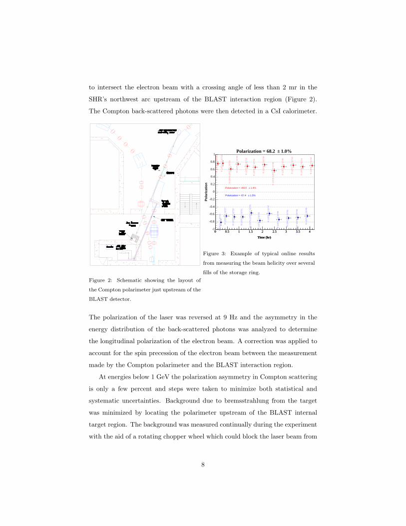
to intersect the electron beam with a crossing angle of less than 2 mr in the

SHR’s northwest arc upstream of the BLAST interaction region (Figure 2).

The Compton back-scattered photons were then detected in a CsI calorimeter.

Figure 2: Schematic showing the layout of

the Compton polarimeter just upstream of the

BLAST detector.

Time (hr)

0 0.5 1 1.5 2 2.5 3 3.5 4

Time (hr)

0 0.5 1 1.5 2 2.5 3 3.5 4

Po

lari

zati

on

-1

-0.8

-0.6

-0.4

-0.2

0

0.2

0.4

0.6

0.8

1

R 1

2574

F 3

2725

R 1

2574

F 3

2727

R 1

2575

F 3

2729

R 1

2575

F 3

2731

R 1

2575

-125

76F

327

33

R 1

2576

F 3

2735

R 1

2576

F 3

2737

R 1

2577

F 3

2739

R 1

2577

F 3

2741

R 1

2577

-125

78F

327

43

R 1

2578

F 3

2745

1.5%±Polarization = -67.4

R 1

2574

F 3

2724

R 1

2574

F 3

2726

R 1

2574

-125

75F

327

28

R 1

2575

F 3

2730

R 1

2575

F 3

2732

R 1

2576

F 3

2734

R 1

2576

F 3

2736

R 1

2576

-125

77F

327

38

R 1

2577

F 3

2740

R 1

2577

F 3

2742

R 1

2578

F 3

2744

R 1

2578

F 3

2746

1.4%±Polarization = +69.0

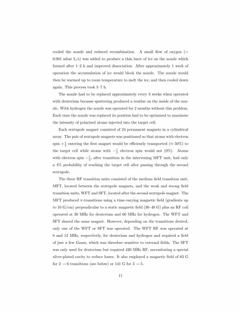
1.0%±Polarization = 68.2

Figure 3: Example of typical online results

from measuring the beam helicity over several

fills of the storage ring.

The polarization of the laser was reversed at 9 Hz and the asymmetry in the

energy distribution of the back-scattered photons was analyzed to determine

the longitudinal polarization of the electron beam. A correction was applied to

account for the spin precession of the electron beam between the measurement

made by the Compton polarimeter and the BLAST interaction region.

At energies below 1 GeV the polarization asymmetry in Compton scattering

is only a few percent and steps were taken to minimize both statistical and

systematic uncertainties. Background due to bremsstrahlung from the target

was minimized by locating the polarimeter upstream of the BLAST internal

target region. The background was measured continually during the experiment

with the aid of a rotating chopper wheel which could block the laser beam from

8

intercepting the electron beam. A movable Pb collimator was used to define

the acceptance of the calorimeter and to minimize background from beam halo.

The readout of the calorimeter was designed to permit linear operation at high

rates and the phototube bases were engineered to minimize saturation effects.

Furthermore, a set of stainless steel absorbers could be inserted remotely to

attenuate the photon flux observed at the highest electron beam currents. This

permitted the polarimeter to operate over a wide range of beam currents ranging

from a few mA to 250 mA. The polarization of the electron beam in a given fill

was usually measured to a statistical precision of around 4% (Figure 3).

The mean longitudinal polarization of the beam during the 2004 BLAST ex-

periment was Pe = 0.66± 0.04. The uncertainty was dominated by systematic

uncertainty in the calibration of the polarimeter. The magnitude of polarization

for the two electron helicity states was the same to better than 1%. This was

verified with the aid of an RF dipole developed to flip adiabatically the helicity

of the stored beam within a fill [17] and helped constrain geometric false asym-

metries in the polarimeter. Although the efficiency in flipping the spin reached

98%, this device introduced additional dead time to the experiment as well as

problems with beam stability at high currents. For this reason, it was used only

occasionally during BLAST operation and reversal of the electron beam helicity

was generally performed at the polarized source prior to each SHR fill.

3. The Atomic Beam Source Internal Target

An atomic beam source [18] (ABS) was used to produce highly polarized,

isotopically pure protons and deuterons in the BLAST target cell aligned with

the electron beam in the South Hall Ring. The ABS was originally designed and

built at NIKHEF [19, 20] but most components were redesigned at MIT-Bates

to accommodate the BLAST environment: primarily the space limitations and

the 2 kG magnetic field in which the ABS was situated.

The ABS, schematically shown in Figures 4 and 5, consisted of:

• an RF dissociator which produced atomic hydrogen or deuterium from the

9

Figure 4: Schematic of the BLAST atomic

beam source, the internal target, and Breit-

Rabi polarimeter.

Figure 5: Location of the ABS elements rel-

ative to the magnetic field in which each op-

erated.

molecular gas,

• four turbo-molecular pumps used to pump the region directly after the

dissociator,

• two sets of permanent sextupole magnets which focused the atomic beam

into the target tube located on the beam axis,

• three RF transition units in combination with magnets to populate selec-

tively the desired polarization states, and

• a Breit-Rabi polarimeter located below the target cell, used to tune and

optimize the ABS transitions.

During operation ∼ 1 mbar L/s of hydrogen or deuterium gas was flowed

through the dissociator. A cold head (70 K) at the exit of the dissociator

10

cooled the nozzle and reduced recombination. A small flow of oxygen (∼

0.001 mbar L/s) was added to produce a thin layer of ice on the nozzle which

formed after 1–2 h and improved dissociation. After approximately 1 week of

operation the accumulation of ice would block the nozzle. The nozzle would

then be warmed up to room temperature to melt the ice, and then cooled down

again. This process took 5–7 h.

The nozzle had to be replaced approximately every 3 weeks when operated

with deuterium because sputtering produced a residue on the inside of the noz-

zle. With hydrogen the nozzle was operated for 2 months without this problem.

Each time the nozzle was replaced its position had to be optimized to maximize

the intensity of polarized atoms injected into the target cell.

Each sextupole magnet consisted of 24 permanent magnets in a cylindrical

array. The pair of sextupole magnets was positioned so that atoms with electron

spin + 12 entering the first magnet would be efficiently transported (≈ 50%) to

the target cell while atoms with − 12 electron spin would not (0%). Atoms

with electron spin − 12 , after transition in the intervening MFT unit, had only

a 4% probability of reaching the target cell after passing through the second

sextupole.

The three RF transition units consisted of the medium field transition unit,

MFT, located between the sextupole magnets, and the weak and strong field

transition units, WFT and SFT, located after the second sextupole magnet. The

MFT produced π-transitions using a time-varying magnetic field (gradients up

to 10 G/cm) perpendicular to a static magnetic field (30–40 G) plus an RF coil

operated at 30 MHz for deuterium and 60 MHz for hydrogen. The WFT and

SFT shared the same magnet. However, depending on the transitions desired,

only one of the WFT or SFT was operated. The WFT RF was operated at

8 and 12 MHz, respectively, for deuterium and hydrogen and required a field

of just a few Gauss, which was therefore sensitive to external fields. The SFT

was only used for deuterium but required 420 MHz RF, necessitating a special

silver-plated cavity to reduce losses. It also employed a magnetic field of 63 G

for 2→ 6 transitions (see below) or 141 G for 3→ 5.

11

The hyperfine structures for hydrogen and deuterium are shown in Figure 6.

Only the upper states (mS = + 12 ) pass through the first sextupole magnet. For

Figure 6: Hyperfine structure of hydrogen (left) and deuterium (right) as a function of the

reduced magnetic field (BHc = 507 G, BD

c = 117 G)

hydrogen the MFT would induce the 2→ 3 transition and only state |1〉 would

be transported to the target cell. The WFT following the second sextupole,

could then be used (or not) to induce the transition 1 → 3 thus selecting the

nuclear polarization for the hydrogen atoms delivered to the target cell. For

deuterium the MFT induced either 3→ 4 or 1→ 4 transitions and then either

the SFT (inducing either 2 → 6 or 3 → 5) or the WFT (1, 2 → 3, 4) would be

used to achieve the desired, nuclearly polarized, deuteron states in the target

cell.

The polarization states used during the experiment and the schemes for op-

erating each unit are given in Tables 1 and 2. For hydrogen the experiment

cycled randomly, but evenly, through the two polarization states, V+ and V−.

For deuterium the experiment cycled randomly, but evenly, through three po-

larization states: one purely tensor, T−, and the other two being combinations

of vector and tensor polarization. This permitted both vector and tensor asym-

metries to be measured efficiently and simultaneously by combining the spin-

12

Name V+ V-

MFT 2→ 3 2→ 3

States |1〉 |1〉

WFT off 1→ 3

State |1〉 |3〉

PZ +1 -1

Table 1: Transition schemes and resulting po-

larization states for hydrogen.

Name V+ V- T-

MFT 3→ 4 3→ 4 1→ 4

States |1〉, |2〉 |1〉, |2〉 |2〉, |3〉

WFT off 1, 2→ 3, 4 off

SFT 2→ 6 off 3→ 5

States |1〉, |6〉 |3〉, |4〉 |2〉, |5〉

PZ +1 -1 0

PZZ +1 +1 -2

Table 2: Transition schemes and resulting po-

larization states for deuterium.

dependent yields appropriately. The spin state was changed every 5 minutes

during the experiment.

The ABS was situated above the BLAST interaction point between the ver-

tical coils of the BLAST toroid. One of the major challenges for operating

the ABS was the external magnetic field which reached values up to 2.2 kG in

the region of the MFT (see Figure 5). This required extensive shielding of the

ABS and careful tuning and monitoring of the transition units to correct for

hysteresis in the ABS magnets.

To assist in tuning the transitions, a Breit-Rabi polarimeter with a dipole

magnet was installed below a small aperture in the target cell. The dipole

magnet transported atoms into one of three compression tubes (left, middle, and

right) depending on their spin state. This permitted the relative populations of

the atomic polarization states and the degree of dissociation to be sampled and

thus optimized.

The target tube was 60 cm long and 1.5 cm in diameter centered on the

beam axis. The tube walls were made from 50 µm aluminum and had open

ends to eliminate background that would be produced by the electron beam

passing through any entrance or exit windows. The target cell was also cooled to

around 100 K and coated with Drifilm to reduce depolarization inside the target

cell. A thick tungsten collimator with 1 cm diameter aperture was situated just

13

upstream of the target cell and served to protect the cell walls from the beam

halo and the injection flash during filling.

In addition to the ABS, an unpolarized gas system with a well-determined

buffer volume could be connected to the target cell. The unpolarized system

was used to make systematic checks of false asymmetries. Also, by measuring

the pressure change in the buffer volume (at constant temperature), the flow,

and thus the density, of unpolarized gas in the target cell could be determined

using the known conductance of the target cell. Comparing the scattering rates

observed with unpolarized to polarized or ABS running permitted the target

density with the ABS to be measured.

The intensity of polarized atoms in the target cell was very sensitive to the

pumping in the ABS. Four turbomolecular pumps operated directly on the vol-

ume around the nozzle and cryopumps were used in the region of the sextupole

magnets. Also, turbomolecular pumps connected to the beamline before and

after the target cell were used to isolate the target from the high vacuum of the

beamline and thus minimize the effect of the target on beam lifetime.

A holding field magnet around the target cell was used to define the nom-

inal spin direction at the center of the target cell. During the experiment the

spin angle was determined from the measured tensor asymmetry in elastic ed

scattering to be 31.3◦ ± 0.43◦ in 2004 and 47.4◦ ± 0.45◦ in 2005, relative to the

beam direction, and horizontal into the left sector. The nominal spin directions

were chosen so electrons scattering into the left sector corresponded to momen-

tum transfers roughly perpendicular to the target spin direction, while electrons

scattering into the right sector had momentum transfers roughly parallel to the

target spin. The spin direction varied slightly along the length of the target

cell (see Figure 7). This was measured by a variety of techniques which yielded

a consistent shape. A parameterization of this shape was used in the analyses

with the value at the center of the target determined from the physics analysis

of elastic scattering from tensor polarized deuterium [21].

Assuming a beam polarization of 66%, polarizations of PZ ≈ 83% were

achieved for hydrogen and PZ ≈ 89% (79%) and PZZ ≈ 69% (55%) for deu-

14

Figure 7: Polarization direction (polar angle in degrees) as a function of position along the

target cell.

terium in 2004 (2005). Target areal densities around 7 × 1013 atoms/cm2 for

both hydrogen and deuterium were typical.

4. The BLAST Detector

The BLAST detector (see Figure 8) was situated on the South Hall Ring

just downstream of the injection point. The detector was based upon an eight

sector, toroidal, magnetic field. The two horizontal sectors were instrumented

with detector components while the two vertical sectors were used by the in-

ternal targets and pumping for the beamline. The detector was left/right sym-

metric with the exception of the neutron detectors which were enhanced in the

right sector (see Section 4.5). Each sector included drift chambers for tracking,

aerogel Cerenkov detectors to discriminate between electrons and pions, time-

of-flight scintillators to determine the relative timing of the reaction products

15

Target

Wire Chambers

Neutron Detectors

Time of Flight

Cerenkov

Toroid Magnet

Figure 8: Schematic of the BLAST detector showing the main detector elements.

and provide the trigger timing, and thick walls of plastic scintillators to iden-

tify neutrons using time-of-flight. The following sections describe the detector

components in greater detail.

4.1. Toroidal Magnet

The toroidal magnet was designed and assembled at MIT-Bates. A toroidal

configuration was chosen to ensure a small field along the beamline to minimize

effects on the beam transport, and also to have small gradients in the region of

the target cell. The magnetic field in the region of the drift chambers was used

to identify the charge and momentum-analyze the charged particles produced

during the experiment. It also minimized the number of low-energy charged

particles reaching the detectors.

16

The toroid consisted of eight copper coils placed symmetrically about the

beamline. Their profile and nominal position relative to the beam line and tar-

get are shown in Figure 9. The unusual shape extended the intense region of

R1 255mm

R3 531.9mm

533.4mm

R4 538mm

R2 430mm

Curve Z X R1 -636.3 1288.4 R2 1938.5 1113.4 R3 1491.0 1215.5 R4 491.0 -38.5

Z

X

Figure 9: Plan view of BLAST coil outline showing dimensions and position relative to the

center of the target cell.

the toroidal magnetic field to forward angles. Each coil consisted of 26 turns of

hollow, 1.5 inch square copper tube organized into two layers of 13 turns. The

copper tubes were wrapped with fiberglass tape and then potted with epoxy

resin. The coils were cooled by flowing water through the hollow conductors.

During the BLAST experiment the normal operating current was 6730 A, re-

sulting in a maximum field of about 3.8 kG.

Before the detectors were installed, the magnetic field was carefully measured

particularly along the beam axis and in the target region [22]. The coil positions

were adjusted to minimize the field along the beamline and gradients at the

target. After this was done a systematic mapping was performed of the magnetic

field in each of the horizontal sectors throughout the volume which would be

occupied by the tracking detector. The results of this mapping were compared

with results from a simple calculation based on the Biot-Savart law as well as a

17

Vector Fields1 TOSCA simulation.

Discrepancies between the measured and calculated field values could be ex-

plained by the uncertainty in the precise conductor positions and by the deflec-

tion of the coils under gravity or when energized. The Biot-Savart calculations

were redone allowing the coil positions to move radially, along the beam direc-

tion, and in azimuthal position to obtain good agreement with the measured

values. These calculated values were then used to extend the mapping to regions

where it was impossible to make a direct measurement. This extended mapping

was used in the reconstruction of events.

4.2. Drift Chambers

The drift chambers measured the momenta, charges, scattering angles, and

vertices for the particles produced in the reactions studied with BLAST. This

was done by tracking the charged particles in three dimensions through the

toroidal magnetic field and reconstructing the trajectories. Measuring the cur-

vature of the tracks yielded the particles’ momenta, and the directions of cur-

vature determined their charge. Tracing the particles’ trajectories through the

mapped magnetic field back to the target region allowed the scattering angles,

polar and azimuthal, to be determined. The position of closest approach to the

beam axis was taken as the vertex position for the event.

To maximize the active area, the drift chambers were designed to fit between

the coils of the toroidal magnet such that the top and bottom plates of the drift

chamber frame were in the shadow of the coils as viewed from the target. The

drift chambers had a large acceptance and nominally subtended the polar an-

gular range 20◦–80◦ and ±15◦ in azimuth with respect to the horizontal plane,

and were orientated such that 73.54◦ with respect to the beam was perpendic-

ular to the face of the chambers. Because of these choices the chambers were

trapezoidal in shape (see Figure 10).

Each sector in BLAST contained three drift chambers (inner, middle, and

1Vector Fields Inc. Aurora, IL, USA

18

Figure 10: Isometric view of all three drift chambers assembled into a single gas volume.

outer) joined together by two interconnecting sections to form a single gas vol-

ume. This was done so that only a single entrance and exit window was required

for the combined drift chambers, thus minimizing energy loss and multiple scat-

tering.

Each of the three chambers consisted of top, bottom, and two end plates.

Each plate was precisely machined from a solid aluminum plate2 and then

pinned and bolted together to form each drift chamber. The positions of the

feedthrough holes (described below) and twelve (12) tooling balls set in inserts

along the length of the top and bottom plates were measured with a coordi-

nate measuring machine, CMM, at Allied Mechanical. These data were used

for quality assurance and for the alignment of the chambers in BLAST. The

chambers were then disassembled and shipped to MIT, where they were cleaned

2Allied Mechanical Ltd., Ontario, CA, USA

19

and reassembled to form the individual chambers. O-rings were used to form a

gas seal. The chambers were wired (described below) separately and then the

three chambers of a sector and the interconnection sections were assembled to

form the complete drift chamber for each sector.

The top and bottom plates of the two interconnecting sections between the

chambers were 18 inch aluminum sheets to be flexible and to conform to the shape

of the connected chambers. The end pieces of the interconnection sections were

rigid and connected to the chambers with pins and bolts to hold the relative

positions of the three drift chambers.

Figure 11 shows a cross sectional view of the top plates for the three drift

Figure 11: Cross sectional view of the top plates of the three drift chambers and the two

interconnecting sections when assembled into a single gas volume.

chambers when assembled. The darker shade shows the top plates for the three

chambers. The lighter shade is used to highlight the recesses which were ma-

chined into both sides of each plate to produce a 7 mm thick section to accom-

modate the feedthroughs for the wires which formed the drift chamber cells.

The thick portions of each plate were needed to resist the combined wire ten-

sions over the length of the drift chamber. Recall that the top and bottom

plates of the frame were in the shadow of the coil as viewed from the interaction

area so the thicknesses shown here did not impact on the detector acceptance.

The frame dimensions were adjusted so that each chamber bowed by approxi-

20

mately the same amount (on the order of 1 mm) due to the wire tension. This

was necessary to simplify connecting the chambers into a single gas volume.

The thin aluminum profile which formed the interconnecting section is visible

along the bottom edge between pairs of chambers. The empty region above the

interconnecting plate was used to hold the amplifier/discriminator electronics,

HV distribution, and for the HV and signal cable runs. The thin line running

along the top of the whole assembly represents a 18 inch copper sheet which was

used to protect the feedthroughs, wires, and electronics. The bottom plates for

the chambers and interconnecting sectors were similar and also had a protective

copper plate.

Each chamber consisted of two super-layers (or rows) of drift cells separated

by 20 mm. The drift cells were “jet-style” formed by wires. Figure 12 shows a

Figure 12: Portion of a chamber showing the two super-layers of drift cells formed by wires.

Lines of electron drift in the drift cells assuming the maximum BLAST field of 3.8 kG are

also shown.

portion of one chamber with the two super-layers of drift cells formed by wires.

It also shows characteristic “jet-style” lines of electron drift in a magnetic field.

Each drift cell was 78×40 mm2 and had 3 sense wires staggered ±0.5 mm from

the center line of each cell to help resolve the left/right ambiguity in determining

position from the drift time. This pattern of wires was realized by stringing wires

21

between the top and bottom plates of each chamber. Holes for each wire were

machined in the thin plate of the recessed areas of the top and bottom plates

to accept Delrin feedthroughs. The feedthrough had a gold plated copper tube

insert through which the wire was strung and crimped. The pin provided a

convenient connector for the HV.

Machining the feedthrough holes was nontrivial. The wires for each super-

layer were inclined at ±5◦ to the vertical. This stereo angle between the front

and back super-layers in each chamber allowed reconstruction in three dimen-

sions. Because of this the hole patterns in the top and bottom plates were not

mirror images but were shifted relative to each other. This was further compli-

cated by the fact that the recessed plate surface was inclined both left to right

and front to back and the hole direction was not perpendicular to either. The

feedthrough holes first had to be spot faced and then drilled and reamed to

produce a press fit for the feedthrough.

Each drift chamber was wired separately. First, the chamber had to be pre-

stressed to the tension that all the wires would exert. This was done by stringing

piano wire through the centre of each drift cell and tensioning these to the to-

tal tension which the real wires would produce. The tension was determined

by plucking the piano wire and measuring the frequency using a microphone

connected to a computer which performed a Fourier analysis. This process was

repeated until all piano wires were properly tensioned. Next, 14 inch clear plas-

tic windows were attached to the front and rear faces of the chamber. This

helped keep the insides of the chamber clean and also protected the wires from

accidents. The chambers were then moved into a clean room for the actual

wiring.

The chambers were wired horizontally. First a wire was strung through a

feedthrough. Then the wire was fastened to a long, hollow stainless steel needle

which was threaded through the holes machined in the top and bottom plates.

Pulling the needle through carried the wire from one side to the other where it

was threaded through another feedthrough. Then the feedthroughs were pushed

into the machined holes. The wire was drawn through the feedthroughs from

22

the supply spool to ensure only clean and straight wire was used. Then the

copper pin of the feedthrough was crimped on one side securing the wire. A

weight was attached to the wire on the other side and stretched over a pulley.

The other pin was then crimped. This process was repeated from one end of

the chamber to the other removing the piano wires as each cell was completed.

Periodically the tensions in the real wires were checked. This was done by

passing DC electrical currents through two neighboring wires. An AC current

was added to one producing an alternating magnetic field in which the other wire

would start to vibrate. Then the AC current was switched off, and the current

induced by the vibrating wire measured and Fourier analyzed to determine the

frequency. Generally two frequencies were measured, one for each wire; but by

measuring different pairs and by the different strengths of the signals, it was

possible to identify each wire’s frequency and hence tension.

When all three chambers of a sector were wired the plastic protective win-

dows were removed and the interconnecting sections installed to join the three

chambers into a single unit. Then the electrical connections were made and

amplifier/discriminator electronics installed.

The completed drift chamber was then optically surveyed. The twelve tool-

ing ball locations on the top and bottom plates of each individual chamber were

measured to determine the relative positions of the three chambers with respect

to each other. Survey targets in bushings on the end plates of all chambers were

also measured.

The drift chamber was then mounted in the sub-detector frame and its posi-

tion and orientation adjusted until it was in its nominal position. This position

was checked with another optical survey of the targets on the end plates. These

data were used together with the previous survey and the data from the CMM

data on the hole positions to determine the position of each sense wire in the

BLAST coordinate system.

With all three drift chambers assembled and positioned, there were 18 planes

of sense wires in each sector with which to track the charged particles produced

at BLAST. In total there were approximately 10,000 wires with 954 sense wires

23

for both sectors in BLAST.

A helium:isobutane gas mixture (82.3:17.7) was chosen for the drift cham-

bers. The chambers were maintained at a pressure of approximately 1 inch of

water above atmospheric pressure with a flow rate of around 3 L/min. The pri-

marily helium mixture had a relatively low density to reduce multiple scattering

and energy loss. Also, because the BLAST toroidal field was inhomogeneous

over the tracking volume, a small Lorentz angle was desirable so that corrections

were small even in regions with high magnetic fields. The helium gas mixture

chosen satisfied this as well with ≈ 7◦ Lorentz angle in a 3.8 kG field. Figure 12

shows the distinctive lines of electron drift, “jets”, for this cell design at 3.8 kG.

Using a single gas volume minimized the number of entrance and exit windows

for the same reason. Two layers of 25 micron mylar were used for the entrance

and exit windows.

4.3. Cerenkov detectors

Immediately behind the drift chambers in each sector were aerogel Cerenkov

detectors [23] designed and produced at Arizona State University to identify

electrons up to 700 MeV/c with 89% efficiency. These detectors were used

to discriminate between pions and electrons which otherwise were not clearly

separated by timing in BLAST. An aerogel Cerenkov detector was chosen to

produce a compact detector and to minimize the energy loss.

Originally there were four Cerenkov detectors in each sector. A schematic

of a Cerenkov box is shown in Figure 13. The boxes contained the aerogel and

supported shielded photomultiplier tubes, PMTs, at both the top and bottom.

The front and back faces of the boxes were made of honeycomb sandwiched

between 1 mm thick aluminum to minimize material while providing support

for the PMTs. The sides were made of 18 inch aluminum sheets. The inside

of each box was painted with Spectraflect3, a white, diffusively reflective paint

which has 96–98% reflectivity for light at a wavelength of 600 nm.

3Labsphere, North Sutton, NH, USA

24

Figure 13: Schematic of a Cerenkov detector box which contained the aerogel and supported

the photomultiplier tubes.

A clear silica aerogel4 was used. The tiles were approximately 11×11×1 cm3

and were laid in rows separated by a strip of mylar (a razor was used to trim

the tiles so they fit snugly). The forward Cerenkov detectors in each sector had

7 layers of aerogel tiles with a refractive index of n = 1.020 while the other

detectors had 5 layers and an index of n = 1.030. The layers of aerogel were

held in place by a thin mylar foil. A photograph of the inside of a detector box

is shown in Figure 14.

The forward-most detector box in each sector had 6 PMTs (3 top, 3 bottom)

while the next had 8 PMTs and the rear two boxes each had 12 PMTs. Five-

inch Photonis5 photomultipliers, XP4500B, were used to collect the Cerenkov

radiation.

4Matsushita Electric Works, Ltd. Osaka, Japan5Photonis USA Inc. Sturbridge, MA, USA

25

Figure 14: Inside view of Cerenkov detector showing white painted box with aerogel and

openings for four PMTs.

The photomultiplier tubes chosen were sensitive to magnetic fields above

0.5 G. The initial shielding design had two concentric iron cylinders of 10 mm

and 6 mm wall thickness separated by an air gap around each tube. However,

measurements inside the cylinders at the location of the PMTs showed a residual

magnetic field on the order of 3–5 G when the BLAST toroid was energized.

Extra iron plates 0.5 inch thick in the forward region and 1 inch thick in the

backward region had to be added between the BLAST toroid and the PMT

enclosures to adequately shield the tubes from the toroid’s fringe field.

During the experiment the rearmost box in each sector was removed to im-

prove the detection of elastically scattered deuterons with the time of flight

scintillators. This fourth box from each sector was used for the BAT detector

(see 4.6). With the remaining three boxes in each sector, an electron identifica-

tion efficiency of 89% was achieved.

26

4.4. Time-of-Flight Scintillators

In each sector 16 vertical scintillator bars formed the time-of-flight (TOF)

detector. The TOF detector was designed and produced at the University of

New Hampshire to provide a fast, stable timing signal correlated with the time

of each event at the target independent of which scintillator bar was struck.

This signal was used to trigger the readout and data acquisition system for

all other components and particularly provided the COMMON STOP signal for

the drift chambers. This permitted relative timings among all components to be

measured. The TOF detector also provided a measure of energy deposition to

aid particle identification. Approximate position information was also possible

from the timing difference between the top and bottom photomultiplier tubes.

The TOF detector curved behind (see Figure 15) the wire chambers and

Figure 15: TOF detector mounted in sub-detector support during assembly.

Cerenkov detectors in each sector, roughly matching the angular coverage of the

tracking detector in both polar (∼ 20◦ < θ <∼ 80◦) and azimuthal (± ∼ 15◦)

27

projections. The forward four bars at θ < 40◦ were 119.4 cm high, 15.2 cm

wide, and 2.54 cm thick. The remaining 12 bars at θ > 40◦ were 180.0 cm high,

26.2 cm wide, and 2.54 cm thick.

Bicron6 BC-408 plastic scintillator was chosen for its fast response time

(0.9 ns rise time) and long attenuation length (210 cm). Each TOF scintillator

bar was read out at both ends via Lucite light guides coupled to 3-inch diameter

Electron Tubes7 model 9822B02 photomultiplier tubes equipped with Electron

Tubes EBA-01 bases. The light guides were bent to point away from the in-

teraction region so the PMTs would be roughly perpendicular to the toroidal

magnetic field. Mu-metal shielding was used around all PMTs. The bases had

actively stabilized voltage dividers so that the timing was independent of the

gain.

With readout from both ends of a TOF scintillator bar, the time difference

provided coarse position information. To provide a timing signal independent

of position along the TOF, the signals from each PMT were split, with one part

from each pair of tubes going to a meantimer. This meantime signal was used to

provide the event timing signal. Because each TOF was at a different distance

from the target center, a delay was added to the closer detectors corresponding

to the time for a relativistic particle to travel the difference in distance. These

time differences were measured for each sector by inserting a thin plastic scintil-

lator paddle near the target chamber and measuring the TOF detector timing

relative to the common start from this paddle. These delayed, meantimed sig-

nals were thus correlated with the time of the event at the target. The signals

from each PMT were also distributed to TDCs and ADCs.

A 2 mm thick Pb foil was placed in front of each TOF bar to attenuate

X-rays from the target region. It also prevented back-scattered radiation from

firing the Cerenkov detector and being mis-identified as electrons. However, the

Pb foil was removed from the four rearmost TOF scintillator bars to improve

6Bicron, Solon, OH, USA7Electron Tubes Ltd, Ruislip, Middlesex, England

28

the sensitivity to low-energy deuterons.

Gains for the PMTs were set by requiring the ADC signal for minimum

ionizing particles from cosmic rays to peak in channel 1250. An intrinsic time

resolution of 320 ± 44 ps was measured for the 32 TOF detectors, which was

significantly better than the 500 ps required by the experiment. Timing offsets

between pairs of scintillator bars were determined using cosmic rays periodically

during the experiment and monitored continuously using the laser flasher system

(section 4.7). The efficiency was determined to be better than 99%.

4.5. Neutron Detectors

Beyond the other detectors were banks of thick scintillator to detect neu-

trons. Three types of neutron detector were employed in BLAST:

Ohio Walls - Two walls approximately 10 × 180 × 400 cm3 situated in both

left and right sectors. Each wall was made using 10 cm thick, 22.5 cm

high, 400 cm long bars of scintillator stacked horizontally with PMTs at

either end.

LADS15 - Two walls approximately 15× 213× 160 cm3, one behind the other

at approximately 35◦ in the right sector. Each wall was made of 14 wedge

shaped scintillator bars, 15 cm thick, 14.5 cm wide (at midpoint of wedge),

and 160 cm high arranged vertically with PMT readout at each end. A

solid wall was formed by alternating the direction of the wedges.

LADS20 - Two walls approximately 20 × 137.2 × 160 cm3positioned parallel

to the beamline, in front of the Ohio wall in the right sector. Each wall

was made of 14 wedge shaped scintillator bars, 20 cm thick, 9.8 cm wide

(at midpoint of wedge), and 1.6 m high arranged vertically with PMT

readout at each end. A solid wall was formed by alternating the direction

of the wedges.

The Ohio Walls were designed and produced at Ohio University using Bicron-

408 scintillator as used in the TOF detector. Similarly the same 3 inch PMTs

and bases as in the TOF detector were used here.

29

The LADS scintillators were originally produced for the Large Acceptance

Detector System [24] at the Paul Scherrer Institute, Switzerland and obtained

from the Jefferson Laboratory, Virginia, USA. Hamamatsu,8 5-inch PMTs were

used to read out the LADS scintillator bars. Bases were developed at MIT-

Bates and UNH with active, transistor-based compensation for the last four

dynodes which permitted a power supply with lower maximum current to be

used. These actively compensated bases had a more stable gain (±5–10%) at

rates up to 800 kHz compared to the usual passive bases (∼ 100% variation).

The neutron detectors were initially gain-matched using cosmic rays and

a dedicated trigger. Later the detection threshold was estimated using the

2.2 MeV endpoint of a 90Sr beta spectrum. For the Ohio Wall this yielded a

threshold of approximately 2.5 MeV for electrons corresponding to 6–7 MeV for

protons. A threshold less than 1 MeV (2.5 MeV) for electrons was obtained

for the 20 cm (15 cm) thick LADS detectors corresponding to approximately

4 MeV (7 MeV) for protons.

A VME-based logic module was developed at MIT-Bates to process the raw

signals from the LADS detectors. This featured leading-edge discrimination

with a prompt and delayed output for each channel, which were connected to

the scalers and TDCs. It also generated a logical AND of top and bottom PMT

pairs with a flexible delay and an OR of all the AND signals which could be

used as a trigger.

The location of the neutron detectors in 2004 is shown in the schematic plan

view of the BLAST detector in Figure 16. The arrangement of neutron detectors

was asymmetric with larger and thicker (more efficient) coverage in the right

sector. This was chosen to improve the BLAST measurement of the neutron

electric form factor GnE which would be more sensitive to neutrons scattering

into the right sector once the deuteron spin vector was chosen to be directed

horizontally into the left sector. The L20 walls tripled the effective detector

thickness of the Ohio wall at low Q2 between 45–90◦. The L15 walls provided

8Hamamatsu, Bridgewater, NJ, USA

30

WCCCTOFLADSNC L20 L15

upstream downstream

2m

Figure 16: Schematic plan view of the BLAST detector configuration during the 2004 running

period.

30 cm of total thickness in the high Q2 region between 25–45◦. In 2005 the left

sector Ohio wall was moved forward to cover 30–80◦.

During running in 2004 it was observed that gammas originating at the

collimator upstream of the BLAST target generated high rates which tripped

the most forward LADS bars. To reduce this rate, 3/8 inch lead sheets were

mounted in front of the L15 detectors. In 2005, 1 inch iron plates were installed

in front of the L15 detectors which acted as both a shield against low energy

photon showers and as a converter for high energy neutrons, enhancing the

neutron detection efficiency.

31

4.6. Backward Angle TOF (BAT) Detector

In order to detect electrons scattered at angles between 90◦ and 110◦ a large

(12 PMTs) Cerenkov box (see 4.3) and four scintillator bars identical to the

large angle TOFs (see 4.4) were mounted at backward angles in both left and

right sectors. These detectors were not combined with any tracking detector nor

backed up with neutron detectors. However, often the scattered proton could

be detected in the main detector and kinematic information determined from

the proton’s scattering angle and momentum could be correlated with events in

the BATs to select ep elastic scattering. Thus the BAT detectors were able to

extend the coverage of BLAST for some reaction kinematics.

4.7. Laser Flasher System

A laser flasher system was used to monitor the timing of all photomulti-

plier based detector systems. A Spectra-Physics9 model VSL-337ND-S ultravi-

olet nitrogen laser was used. The laser output was split into numerous, equal

length fiber optic cables and connected to the centers of each scintillator bar or

Cerenkov box. The laser output was attenuated to be within the ADC range for

each detector. A flasher trigger for the data acquisition system was generated

by connecting a fiber to a photodiode.

Timing calibration measurements were carried out using the laser flasher

system. Since flasher events occur simultaneously in all detectors, the position

of the flasher peak in the TDC is a measure of the offset introduced by the TDC

device and by the length of cables and processing times.

The laser was pulsed at approximately 1 Hz during data taking and the data

acquisition system recorded a FLASHER event for all detector components.

These events could be analyzed to track changes in the timing of any detector

channel with time. Since all scintillator bars were read out at both ends and

each Cerenkov box had several PMTs, the flasher data could also be used to

determine the relative time offsets between signals within a detector.

9Spectra-Physics, Mountain View, CA, USA

32

In the case of a leading-edge discriminator, the change in time with signal

amplitude (walk) could also be calibrated by varying the amplitude of the laser

signal. By correlating the ADC and TDC spectrum for each channel the walk

effect could be accounted for on an event-by-event basis.

The timing offsets determined with the flasher were subject to drifts over long

periods of time due to variations in the laser strength or when the light fibers

were moved. The relative offset between pairs of scintillators were periodically

generated by measuring the time correlation of cosmic ray events. Between

these dedicated cosmic ray measurements the flasher-triggered data were used

to monitor the timing offsets on a run-by-run basis.

4.8. Electronics

The amplifier/discriminator cards used on the drift chambers produced an

ECL signal for each sense wire. A shielded, 32 conductor, twisted pair cable was

used to carry these signals. The front end electronics for each scintillator and

Cerenkov detector consisted of the photomultiplier tube bases which produced

an analog signal for each channel. These signals were transported to the data

acquisition and trigger electronics via RG58 coaxial cables. All these cables were

approximately 45 m in length though the cables used for the wire chambers were

made as short as possible to minimize attenuation. The analog PMT signals

were attenuated by approximately a factor of two.

The data acquisition and trigger electronics were situated in the “D” tunnel

near the BLAST experiment. This area could be accessed while the experiment

was running to examine signals, check timing, or diagnose and fix problems with

the electronics. The detector high voltage supplies were also housed here.

The drift chamber ECL signal cables were directly connected to LeCroy10

1877S TDCs located in BiRa11 Fastbus crates. One Fastbus crate was used for

each sector of BLAST.

10LeCroy Corp., Chestnut Ridge, NY, USA11BiRa Systems, Albuquerque, NM

33

The signal from each scintillator PMT was sent through a passive analog

splitter. Signals from the PMTs for each Cerenkov box were first combined

using a CAEN12 N402 analog adder and the output was then sent to a splitter.

For each splitter, one of the outputs was sent as a prompt signal to the trigger

logic electronics while the other was delayed by approximately 500 ns using an

analog delay chip in a passive delay chip13 and connected to ADCs (LeCroy

1881) in the Fastbus crates.

4.9. Trigger

The trigger system used at BLAST was based on a similar design for the

Jefferson Laboratory Hall A twin high resolution spectrometers, redesigned for

the BLAST experiment. A schematic for the detectors in one sector is shown

in Figure 17.

The prompt signals from the TOF and BAT detectors were sent to LeCroy

constant fraction discriminators, CFDs, while those from the Cerenkov detectors

went to LeCroy leading edge discriminators, LEDs, and those from the neutron

detectors went to leading edge discriminators designed at MIT-Bates. Outputs

from each discriminator were connected to scalers and to LeCroy 1875 TDCs

in the Fastbus crates after appropriate delays in a PEC delay module to ensure

proper timing. In addition, pairs of discriminator outputs, corresponding to the

top and bottom (or left and right) PMTs of the TOF or neutron detectors, were

connected to AND logic modules to generate a coincidence signal.

Outputs from the AND units were passed to a Memory Lookup Unit, MLU,

for each sector which could be programmed to require different combinations

of input signals to produce an output. Since the MLU only allowed 16 inputs

it was necessary to combine some of the AND outputs. The ANDs of the four

most forward TOF detectors were used separately but the remaining 12 TOFs

(in the sector) were combined in pairs in an OR unit to produce 6 inputs to

12CAEN Technologies, Inc., Staten Island, NY, USA13Paulus Engineering Co., London, TN

34

CFD

CFD

AND

Back AngleTOFs (BATS)

ScintillatorDetectors (TOFs) 1-16

T1-16->1-16

1-16->1-16 B

PER SECTOR

GATES &STARTS

MLU

FINAL LOGIC

delay/FO

delay/FO

to scalerto TDC

to scalerto TDC

3420

3420

4518 /100

4518 /100

4516A1-16

B1-16

AND

4516 CFD

delay/FO delay/FO

3420 4518 /100

4518 /100

A1-8

B1-8

T1-4->1-4

B1-4->1-4

1-8

2373

MLU

2373

From Other Sector

delay/FO

4518 /100

OR

4564

1-4

5-16

Retiming Delay

Delay

to ADCs

to ADCs

to ADCs

to ADCs

PAIROR

4532

OR

4564

to scaler

Flasher

1-4

5-10

11

12

16

1-6

7-12

15

C 561mean-timer

delay

delay

*

*

*

*

note: * all analog signal division in matched impedance passive splitters

LE Disc X8

to ADCs

to ADCs

*

*

AND X8

OR

to scalers

Miro Module

TS

to scalers

to TDCs

NeutronDetectors

2nd Level Trigger(diagram on next page)

from other sector

scalerTDC

delay

C 561mean-timer

to scaler

to TDC

discrCerenkovDetectors 1-4

3412

1-12 delay/FO

4518 /100

to ADCs

CAEN N40724 chadder

2 units

2X10ns

delay

PAIROR

4532

scalerTDC

delay

*

Figure 17: Schematic diagram for the BLAST trigger system.

the MLU. All Cerenkov detectors in a sector were OR’ed to provide a single

MLU input. Similarly the ANDs of the four BAT TOF detectors were OR’ed to

form another input and the AND of all neutron detector signals in a sector were

OR’ed and formed another MLU input. The MLU for each sector produced six

programmable outputs. These six outputs from each sector were then combined

in a “cross” MLU, XMLU, which also accepted the flasher signal as a thirteenth

input.

By programming which inputs to the sector MLUs produced which out-

puts and similarly programming the XMLU, the BLAST trigger could be pro-

grammed to recognize 8 classes of events, which roughly selected the event

35

characteristics of interest for the experiment.

Output from the XMLU was passed to the Trigger Supervisor, TS, custom

designed and built by Jefferson Laboratory. The TS also received as input a

trigger timing signal and a signal from the second level trigger logic described

below. The TS was responsible for producing the COMMON START or COM-

MON STOP (drift chamber) to the TDCs and the gate to the ADCs for readout.

The TS also communicated with the data acquisition system when an event was

ready to be read out. It was also possible to apply prescale factors to the various

event types with the TS.

In order to provide a trigger timing signal related to the time of the event at

the target, the signals from the various TOF detectors were delayed as described

in section 4.4. In the trigger logic the discriminated TOF signals for the top

and bottom PMTs were sent to a meantimer which produced an averaged time,

independent of where the particle struck along the length of the TOF scintillator

bar. The OR of the meantimes of all the TOFs in both sectors was connected

to the trigger supervisor and used to define the timing for the data acquisition

gates and common starts and stops for the TDCs.

A second level trigger (shown in Figure 18) was formed from outputs on the

OR

AND

AND

AND

AND

PHYS0

TS L1A

GATE Gen

GATE Gen

GATE Gen

GATE Gen

GATE Gen

AND

AND

OR

AND

GATE Gen

AND

WC TDC STOP

TS L2P

TS L2FTS L2S

Miro L and R

Miro L

L MLU

Miro R

R MLU

NOT PHYS0

PHYS0

PHYSn n>0

2nd Level Trigger

Figure 18: Schematic diagram for the BLAST second level trigger.

36

back of the LeCroy 1877S TDCs used by the drift chamber. This hit information

was combined in specially designed logic boards to identify events which had

good tracking information by requiring at least one hit in each of the three drift

chambers in a sector which also had a TOF hit (i.e. a charged particle). This

signal was one of the inputs to the trigger supervisor and reduced the trigger

rate by approximately a factor of ten and removed a large number of random

or noise events from the data stream.

4.10. Data Acquisition System

Motorola MV162 (2004) and PowerPC (2005) single-board computers in each

of the Fastbus crates served as readout controllers, ROCs, for each crate. Each

ROC was a Motorola MVME5110-2263 Power PC running VxWorks 5.4 and

connected to the BLAST data acquisition system via Ethernet and was based

in a Struck14 VME to Fastbus Interface.

BLAST used the CEBAF Online Data Acquisition system, CODA, devel-

oped at Jefferson Laboratory. CODA consists of several components which

handle the various stages in data acquisition. When the trigger supervisor indi-

cated a valid event, CODA read the ADCs and TDCs via Ethernet through the

ROCs and passed the data to the event builder, EB. The event builder assem-

bled the data and verified that each piece came from the same trigger. From the

EB, data were passed to event transport, ET, which added other data streams

such as scaler, slow control, and Compton polarimeter information. The ET

also permitted the data to be monitored by sampling (spying) a fraction of the

events which could be analyzed online. The event recorder, ER, wrote the data

to disk.

A graphical user interface to CODA called Run Control allowed the user to

establish communication with the ROCs, set trigger configurations, start and

stop runs, and monitor event rates and sizes.

Buffered readout of the BLAST detector occurred at event rates up to

14Struck Innovative Systeme, Hamburg, Germany

37

1.4 kHz (0.2–0.8 kHz typical) with an event size of ∼ 1.5 kB. Typical dead-

time was less than 10%. Online analysis programs used ET to access a sample

of events and display histograms of raw ADC and TDC information and calcu-

lated quantities such as event vertex.

Struck SIS 3600 scalers were used to count hits in the various PMTs, as well

as rates for the various event types. The scaler modules were located in a VME

crate, along with an SIS 3800 input register that recorded status bits indicating

ABS target species and polarization as well as the electron beam helicity. The

scalers were read out at 1 Hz by a stand-alone program which supplied these

data to the ET and to a visual display. The Computer Automated Measurement

and Control, CAMAC interface was also located in this VME crate.

4.11. Slow Control System

In addition to the detector electronics, trigger, and data acquisition system,

successful operation of the BLAST experiment relied on numerous other com-

ponents which had to be controlled, monitored, and recorded. These included

the high voltages for the PMTs and drift chambers, low voltage power supplies,

the gas system for the drift chambers, pressures and temperatures in the drift

chambers and ABS, the electron beam current in the ring, event rates in the

beam halo monitors, the Compton polarimeter, etc. These diverse components

and bits of information were all organized using the Experimental Physics and

Industrial Control System, EPICS15.

EPICS is a set of software tools and applications which can be run on almost

any computer to provide an infrastructure for building a distributed control sys-

tem. Such systems typically comprise numerous computers, networked together

to allow communication, control, and feedback of the devices connected to each

computer. The EPICS system used at BLAST was integrated with the data

acquisition system and the slow control data was written as part of the normal

event stream and thus readily available during the analyses.

15http://www.aps.anl.gov/epics/index.php

38

5. Operation

During normal operation the accelerator, target, detector, and data acquisi-

tion operated automatically, requiring very little human intervention. When the

current in the storage ring dropped below a preset limit, a signal would instruct

the data acquisition system to stop taking data and to ramp down the high

voltage on all detector components. Once the high voltages were at safe levels,

the beam in the storage ring would be dumped and a new injection started. Af-

ter sufficient current was again stored in the ring, the experiment would ramp

up the high voltage and data taking would resume. This process can be seen

graphically in Figure 19. Typically, the experimental down-time during this

Figure 19: Plot of stored beam current (upper curves) and lifetime (lower curves) over a 30

minute period showing three successive beam fills. The typically fill shown starts with 225 mA

and ends with 165 mA of stored beam while the electron beam lifetime starts at 24 minutes

and gradually improves to 30 minutes.

process was about 90 seconds with data taking running for 10 minute periods.

The beam helicity would be reversed for each fill. The dump current value was

39

chosen to maximize the integrated beam current used by the experiment.

The operation of the experiment was made significantly easier by the instal-

lation of beam quality monitors (BQM) just downstream of the BLAST target

region, and by a tungsten collimator approximately 50 cm upstream from the

target. The collimator served the dual purpose of protecting the target cell

walls from the beam halo and helping reduce background in the wire chambers.

The BQM were a set of four small scintillators with PMT readout situated sym-

metrically around the beampipe. These were used in tuning the beam through

the target and in setting the beam scraper slits. The combined effects of the

collimator, beam tuning, and selective first and second level triggers resulted in

very clean events with minimal background.

The target spin states were randomly cycled independent of the beam or data

acquisition with a different spin state every 5 minutes. The ABS would inhibit

data acquisition for the approximately 2 seconds required for the transition.

Periodically runs were taken with the ABS switched off (i.e. empty target

runs) to provide a measure of the background rates and processes. Similarly, an

unpolarized gas system with a calibrated buffer system was used periodically to

check the unpolarized asymmetries due to irregularities in the detector symme-

try or efficiencies. The unpolarized system also provided a target with a known

density as a check on the luminosity measurement.

Cosmic ray data were also collected and used to check relative timing be-

tween detectors. These data were generally collected during special runs on

maintenance days or at times when the accelerator or target were unavailable.

Cosmic events could also be distinguished within the regular data taking runs

and used as well to monitor performance.

6. Summary

Between 2003 and 2005 the BLAST experiment successfully took data at the

MIT-Bates Linear Accelerator Center. The experiment used a highly-polarized

(66% typical) electron beam of 850 MeV stored in the South Hall Ring. The

40

polarization in the ring was monitored on-line using a Compton polarimeter. An

atomic beam source provided highly-polarized internal gas targets of hydrogen

(PZ ≈ 83%) and deuterium (PZ ≈ 89% (79%) and PZZ ≈ 69% (55%) in 2004

(2005)). A large acceptance, symmetric detector system based on a toroidal

magnetic spectrometer with drift chambers for tracking, aerogel Cerenkov de-

tectors for electron/pion discrimination, time-of-flight scintillators for triggering

and relative timing, thick scintillators for neutron detection and a flexible trig-

ger and data acquisition system was used to study numerous reaction channels

simultaneously. The experiment was explicitly designed and operated to mini-

mize systematic errors by being left/right symmetric and by frequently reversing

the beam helicity and target spin states.

The analyses of the data collected by the BLAST experiment concentrate

on asymmetry measurements and are therefore insensitive to the beam intensity

and target densities and have reduced uncertainties due to detector efficiencies.

These analyses are providing improved measurements for neutron [25, 26, 27,

28], proton [29, 30, 31], and deuteron [21, 32] form factors and allow the spin-

dependent electromagnetic interaction on few-nucleon systems [33, 34] to be

studied in a systematic manner.

This paper has provided a technical description of the accelerator, internal

target, detector, electronics, and operation of the BLAST experiment. A fu-

ture paper will detail the calibration, reconstruction, and performance of the

detector.

7. Acknowledgments

The successful design, construction, and operation of the BLAST experiment

would not have been possible without the research and technical support staffs

of all the institutions involved. In particular we would like to acknowledge

the MIT-Bates accelerator group for providing the high quality electron beam

delivered to the experiment and the MIT-Bates research and engineering support

groups for assembling and maintaining the detector and necessary infrastructure

41

over the many years. We would also like to acknowledge Prof. W. Haeberli for

his advice and support with the internal gas target.

References

[1] R. Alarcon, R. Milner (Eds.), Electronuclear Physics with Internal Targets

and the BLAST Detector, World Scientific, Singapore, 1998, proceedings,

2nd Workshop, Cambridge, USA, May 28-30.

[2] BLAST Collaboration, BLAST Technical Design Report, Tech. rep., MIT-

Bates Linear Accelerator Center (1997).

[3] D. T. Spayde, et al., Parity Violation in Elastic Electron-Proton Scattering

and the Proton’s Strange Magnetic Form Factor, Phys. Rev. Lett. 84 (6)

(2000) 1106–1109. arXiv:nucl-ex/9909010.

[4] T. M. Ito, et al., Parity-Violating Electron Deuteron Scattering and the

Proton’s Neutral Weak Axial Vector Form Factor, Phys. Rev. Lett. 92 (10)

(2004) 102003. arXiv:nucl-ex/0310001.

[5] E. Beise, M. Pitt, D. Spayde, The SAMPLE Experiment and Weak Nucleon

Structure, Progress in Particle and Nuclear Physics 54 (1) (2005) 289–350.

[6] Z. Zhou, et al., Performance of a Compact Detector Package for the Out-of-

Plane Spectrometer System, Nuclear Instruments and Methods in Physics

Research A 487 (2002) 365–380.

[7] D. T. Pierce, F. Meier, Photoemission of Spin-Polarized Electrons from

GaAs, Phys. Rev. B 13 (12) (1976) 5484–5500.

[8] M. Farkhondeh, W. Franklin, E. Tsentalovich, T. Zwart, E. Ihloff, MIT-

Bates Polarized Source, in: Y. Makdisi, A. Luccio, W. Mackay (Eds.), AIP

Conf. Proc. 675: SPIN 2002, Vol. 675 of American Institute of Physics

Conference Series, 2003, pp. 1098–1102.

42

[9] D. Cheever, M. Farkhondeh, W. Franklin, E. Tsentalovich, T. Zwart, High

Power Diode Laser System for SHR, in: Y. Makdisi, A. Luccio, W. Mackay

(Eds.), AIP Conf. Proc. 675: SPIN 2002, Vol. 675 of American Institute of

Physics Conference Series, 2003, pp. 1019–1023.

[10] T. Maruyama, E. L. Garwin, R. Prepost, G. Zapalac, Electron-Spin Polar-

ization in Photoemission from Strained GaAs Grown on GaAs1−xPx, Phys.

Rev. B 46 (7) (1992) 4261–4264.

[11] M. Farkhondeh, E. Tsentalovich, T. Zwart, E. Ihloff, New Results from the

MIT-Bates Polarized Source and the Test Beam Setup, in: K. Hatanaka,

T. Nakano, K. Imai, H. Ejiri (Eds.), AIP Conf. Proc. 570: SPIN 2000, Vol.

570, 2001, p. 955.

[12] T. Zwart, et al., Transmission Polarimetry at MIT Bates, in: Y. Makdisi,

A. Luccio, W. Mackay (Eds.), AIP Conf. Proc. 675: SPIN 2002, Vol. 675

of American Institute of Physics Conference Series, 2003, pp. 1011–1015.

[13] T. Zwart, E. Booth, F. Casagrande, K. Dow, M. Farkhondeh, W. Franklin,

E. Ihloff, K. Jacobs, J. Matthews, R. Milner, T. Smith, C. Tschalaer,

E. Tsentalovich, W. Turchinetz, F. Wang, Polarized Electrons at Bates:

Source to Storage Ring, in: American Institute of Physics Conference Se-

ries, Vol. 588 of American Institute of Physics Conference Series, 2001, pp.

343–349.

[14] W. A. Franklin, The MIT-Bates Compton Polarimeter for the South Hall

Ring, in: 16th International Spin Physics Symposium (SPIN 2004), Trieste,

Italy, 2004, p. 714.

[15] D. P. Barber, et al., The HERA Polarimeter and the First Observation

of Electron Spin Polarization at HERA, Nucl. Instrum. Meth. A 329 (1-2)

(1993) 79–111.

[16] I. Passchier, et al., A Compton Backscattering Polarimeter for Measuring

43

Longitudinal Electron Polarization, Nucl. Instrum. Meth. A 414 (1998)

446–458. arXiv:physics/9902011.

[17] V. S. Morozov, et al., Spin-Flipping Polarized Electrons, Phys. Rev. ST

Accel. Beams 4 (2001) 104002.

[18] D. Cheever, et al., A Highly Polarized Hydrogen / Deuterium Internal Gas

Target Embedded in a Toroidal Magnetic Spectrometer, Nucl. Instrum.

Meth. A556 (2006) 410–420.

[19] M. Ferro-Luzzi, et al., Measurement of Tensor Analyzing Powers for Elastic

Electron Scattering from a Polarized 2H Target Internal to a Storage Ring,

Phys. Rev. Lett. 77 (13) (1996) 2630–2633.

[20] L. van Buuren, D. Szczerba, J. van den Brand, H. Bulten, M. Ferro-Luzzi,

S. Klous, H. Kolster, J. Lang, F. Mul, H. Poolman, M. Simani, Performance

of a Hydrogen/Deuterium Polarized Gas Target in a Storage Ring, Nucl.

Instrum. Methods A 474 (2001) 209–223.

[21] C. Zhang, Measurement of Tensor Analyzing Powers in Elastic Electron

Deuteron Scattering with BLAST, Ph.D. thesis, Massachusetts Institute of

Technology (May 2006).

[22] K. Dow, et al., Magnetic Field Measurements of the BLAST Spectrometer,

to be published.

[23] B. Tonguc, R. Alarcon, T. Botto, J. Calarco, A. Degrush, O. Filoti, E. Geis,

J. Kelsey, J. Prince, E. Six, C. Vidal, The BLAST Cherenkov detectors,

Nucl. Instrum. Methods A 553 (1-2) (2005) 364–369.

[24] T. Alteholz, et al., A Large Acceptance Detector System (LADS) for Stud-

ies of Pion Absorption, Nucl. Instrum. Meth. A373 (1996) 374–386.

[25] V. Ziskin, Measurement of the Electric Form Factor of the Neutron at Low

Momentum Transfers Using a Vector Polarized Deuterium Gas Target at

BLAST, Ph.D. thesis, Massachusetts Institute of Technology (Apr 2005).

44

[26] N. Meitanis, A Measurement of the Neutron Magnetic Form Factor GnM

from Quasi-elastic 2 ~H(~e, e′) and low Q2, Ph.D. thesis, Massachusetts Insti-

tute of Technology (Mar 2006).

[27] E. Geis, The Electric Form Factor of the Neutron at Low Momentum Trans-

fers as Measured at Bates Large Acceptance Spectrometer Toroid, Ph.D.

thesis, Arizona State University (May 2007).

[28] E. Geis, et al., The Charge Form Factor of the Neutron at Low Momentum

Transfer from the 2~H(~e, e′n)p Reaction, Phys. Rev. Lett. 101 (2008) 042501.

arXiv:0803.3827.

[29] C. Crawford, Precision Measurement of the Proton Electric to Magnetic

Form Factor Ratio with BLAST, Ph.D. thesis, Massachusetts Institute of

Technology (May 2005).

[30] A. Sindile, Proton Form Factor Ratio Measurement with BLAST, Ph.D.

thesis, University of New Hampshire (May 2006).

[31] C. B. Crawford, et al., Measurement of the Proton’s Electric to Magnetic

Form Factor Ratio from 1 ~H(~e, e′p), Phys. Rev. Lett. 98 (5) (2007) 052301.

arXiv:nucl-ex/0609007.

[32] P. Karpius, Vector Polarization Observables of the Deuteron and A New

Measurement of the Magnetic Dipole Form Factor GM , Ph.D. thesis, Uni-

versity of New Hampshire (Dec 2005).

[33] A. Maschinot, Analysis of Scattered Protons in Deuteron Electrodisinte-

gration with a Polarized Electron Beam and an Internal Polarized Target,

Ph.D. thesis, Massachusetts Institute of Technology (Sep 2005).

[34] O. Filoti, Inclusive Scattering of Polarized Electrons from Polarized Protons

in the ∆-Excitation Region with BLAST, Ph.D. thesis, University of New

Hampshire (Apr 2007).

45