the black-scholes model - columbia universitymh2078/foundationsfe/blackscholes.pdf · 2 the...

IEOR E4706: Foundations of Financial Engineering c© 2016 by Martin Haugh

The Black-Scholes Model

In these notes we will use Ito’s Lemma and a replicating argument to derive the famous Black-Scholes formulafor European options. We will also discuss the weaknesses of the Black-Scholes model and geometric Brownianmotion, and this leads us directly to the concept of the volatility surface which we will discuss in some detail.We will also derive and study the Black-Scholes Greeks and discuss how they are used in practice to hedgeoption portfolios.

1 The Black-Scholes Model

We are now able to derive the Black-Scholes PDE for a call-option on a non-dividend paying stock with strike Kand maturity T . We assume that the stock price follows a geometric Brownian motion so that

dSt = µSt dt + σSt dWt (1)

where Wt is a standard Brownian motion. We also assume that interest rates are constant so that 1 unit ofcurrency invested in the cash account at time 0 will be worth Bt := exp(rt) at time t. We will denote byC(S, t) the value of the call option at time t. By Ito’s lemma we know that

dC(S, t) =

(µSt

∂C

∂S+∂C

∂t+

1

2σ2S2 ∂

2C

∂S2

)dt + σSt

∂C

∂SdWt (2)

Let us now consider a self-financing trading strategy where at each time t we hold xt units of the cash accountand yt units of the stock. Then Pt, the time t value of this strategy satisfies

Pt = xtBt + ytSt. (3)

We will choose xt and yt in such a way that the strategy replicates the value of the option. The self-financingassumption implies that

dPt = xt dBt + yt dSt (4)

= rxtBt dt+ yt (µSt dt + σSt dWt)

= (rxtBt + ytµSt) dt + ytσSt dWt. (5)

Note that (4) is consistent with our earlier definition of self-financing. In particular, any gains or losses on theportfolio are due entirely to gains or losses in the underlying securities, i.e. the cash-account and stock, and notdue to changes in the holdings xt and yt.Returning to our derivation, we can equate terms in (2) with the corresponding terms in (5) to obtain

yt =∂C

∂S(6)

rxtBt =∂C

∂t+

1

2σ2S2 ∂

2C

∂S2. (7)

If we set C0 = P0, the initial value of our self-financing strategy, then it must be the case that Ct = Pt for all tsince C and P have the same dynamics. This is true by construction after we equated terms in (2) with thecorresponding terms in (5). Substituting (6) and (7) into (3) we obtain

rSt∂C

∂S+

∂C

∂t+

1

2σ2S2 ∂

2C

∂S2− rC = 0, (8)

The Black-Scholes Model 2

the Black-Scholes PDE. In order to solve (8) boundary conditions must also be provided. In the case of ourcall option those conditions are: C(S, T ) = max(S −K, 0), C(0, t) = 0 for all t and C(S, t)→ S as S →∞.

The solution to (8) in the case of a call option is

C(S, t) = StΦ(d1) − e−r(T−t)KΦ(d2) (9)

where d1 =log(St

K

)+ (r + σ2/2)(T − t)σ√T − t

and d2 = d1 − σ√T − t

and Φ(·) is the CDF of the standard normal distribution. One way to confirm (9) is to compute the variouspartial derivatives using (9), then substitute them into (8) and check that (8) holds. The price of a Europeanput-option can also now be easily computed from put-call parity and (9).

The most interesting feature of the Black-Scholes PDE (8) is that µ does not appear1 anywhere. Note that theBlack-Scholes PDE would also hold if we had assumed that µ = r. However, if µ = r then investors would notdemand a premium for holding the stock. Since this would generally only hold if investors were risk-neutral, thismethod of derivatives pricing came to be known as risk-neutral pricing.

1.1 Martingale Pricing

It can be shown2 that the Black-Scholes PDE in (8) is consistent with martingale pricing. In particular, if wedeflate by the cash account then the deflated stock price process, Yt := St/Bt, must be a Q-martingale whereQ is the EMM corresponding to taking the cash account as numeraire. It can be shown that the Q-dynamics ofSt satisfy3

dSt = rSt dt + σSt dWQt (10)

where WQt is a Q-Brownian motion. Note that (10) implies

ST = Ste(r−σ2/2)(T−t)+σ(WQ

T −WQt )

so that ST is log-normally distributed under Q. It is now easily confirmed that the call option price in (9) alsosatisfies

C(St, t) = EQt

[e−r(T−t) max(ST −K, 0)

](11)

which is of course consistent with martingale pricing.

1.2 Dividends

If we assume that the stock pays a continuous dividend yield of q, i.e. the dividend paid over the interval(t, t+ dt] equals qStdt, then the dynamics of the stock price can be shown to satisfy

dSt = (r − q)St dt + σSt dWQt . (12)

In this case the total gain process, i.e. the capital gain or loss from holding the security plus accumulateddividends, is a Q-martingale. The call option price is still given by (11) but now with

ST = Ste(r−q−σ2/2)(T−t)+σ(WQ

T −WQt ).

1The discrete-time counterpart to this observation was when we observed that the true probabilities of up-moves and down-moves did not have an impact on option prices.

2We would need to use stochastic calculus tools that we have not discussed in these notes to show exactly why the Black-Scholes call option price is consistent with martingale pricing. It can also be shown that the Black-Scholes model is completeso that there is a unique EMM corresponding to any numeraire.

3You can check using Ito’s Lemma that if St satisfies (10) then Yt will indeed be a Q-martingale.


In this case the call option price is given by

C(S, t) = e−q(T−t)StΦ(d1) − e−r(T−t)KΦ(d2) (13)

where d1 =log(St

K

)+ (r − q + σ2/2)(T − t)

σ√T − t

and d2 = d1 − σ√T − t.

Exercise 1 Follow the replicating argument given above to derive the Black-Scholes PDE when the stock paysa continuous dividend yield of q.

2 The Volatility Surface

The Black-Scholes model is an elegant model but it does not perform very well in practice. For example, it iswell known that stock prices jump on occasions and do not always move in the continuous manner predicted bythe GBM motion model. Stock prices also tend to have fatter tails than those predicted by GBM. Finally, if theBlack-Scholes model were correct then we should have a flat implied volatility surface. The volatility surface is afunction of strike, K, and time-to-maturity, T , and is defined implicitly

C(S,K, T ) := BS (S, T, r, q,K, σ(K,T )) (14)

where C(S,K, T ) denotes the current market price of a call option with time-to-maturity T and strike K, andBS(·) is the Black-Scholes formula for pricing a call option. In other words, σ(K,T ) is the volatility that, whensubstituted into the Black-Scholes formula, gives the market price, C(S,K, T ). Because the Black-Scholesformula is continuous and increasing in σ, there will always4 be a unique solution, σ(K,T ). If the Black-Scholesmodel were correct then the volatility surface would be flat with σ(K,T ) = σ for all K and T . In practice,however, not only is the volatility surface not flat but it actually varies, often significantly, with time.

Figure 1: The Volatility Surface

4Assuming there is no arbitrage in the market-place.


In Figure 1 above we see a snapshot of the5 volatility surface for the Eurostoxx 50 index on November 28th,2007. The principal features of the volatility surface is that options with lower strikes tend to have higherimplied volatilities. For a given maturity, T , this feature is typically referred to as the volatility skew or smile.For a given strike, K, the implied volatility can be either increasing or decreasing with time-to-maturity. Ingeneral, however, σ(K,T ) tends to converge to a constant as T →∞. For T small, however, we often observean inverted volatility surface with short-term options having much higher volatilities than longer-term options.This is particularly true in times of market stress.

It is worth pointing out that different implementations6 of Black-Scholes will result in different implied volatilitysurfaces. If the implementations are correct, however, then we would expect the volatility surfaces to be verysimilar in shape. Single-stock options are generally American and in this case, put and call options will typicallygive rise to different surfaces. Note that put-call parity does not apply for American options.

Clearly then the Black-Scholes model is far from accurate and market participants are well aware of this.However, the language of Black-Scholes is pervasive. Every trading desk computes the Black-Scholes impliedvolatility surface and the Greeks they compute and use are Black-Scholes Greeks.

Arbitrage Constraints on the Volatility Surface

The shape of the implied volatility surface is constrained by the absence of arbitrage. In particular:

1. We must have σ(K,T ) ≥ 0 for all strikes K and expirations T .

2. At any given maturity, T , the skew cannot be too steep. Otherwise butterfly arbitrages will exist. Forexample fix a maturity, T and consider put two options with strikes K1 < K2. If there is no arbitrage thenit must be the case (why?) that P (K1) < P (K2) where P (Ki) is the price of the put option with strikeKi. However, if the skew is too steep then we would obtain (why?) P (K1) > P (K2).

3. Likewise the term structure of implied volatility cannot be too inverted. Otherwise calendar spreadarbitrages will exist. This is most easily seen in the case where r = q = 0. Then, fixing a strike K, we canlet Ct(T ) denote the time t price of a call option with strike K and maturity T . Martingale pricing impliesthat Ct(T ) = Et[(ST −K)+]. We have seen before that (ST −K)+ is a Q-submartingale and nowstandard martingale results can be used to show that Ct(T ) must be non-decreasing in T . This would beviolated (why?) if the term structure of implied volatility was too inverted.

In practice the implied volatility surface will not violate any of these restrictions as otherwise there would be anarbitrage in the market. These restrictions can be difficult to enforce, however, when we are “bumping” or“stressing” the volatility surface, a task that is commonly performed for risk management purposes.

Why is there a Skew?

For stocks and stock indices the shape of the volatility surface is always changing. There is generally a skew,however, so that for any fixed maturity, T , the implied volatility decreases with the strike, K. It is mostpronounced at shorter expirations. There are two principal explanations for the skew.

1. Risk aversion which can appear as an explanation in many guises:

(a) Stocks do not follow GBM with a fixed volatility. Instead they often jump and jumps to the downsidetend to be larger and more frequent than jumps to the upside.

(b) As markets go down, fear sets in and volatility goes up.

(c) Supply and demand. Investors like to protect their portfolio by purchasing out-of-the-money puts andso there is more demand for options with lower strikes.

5Note that by put-call parity the implied volatility σ(K,T ) for a given European call option will be also be the impliedvolatility for a European put option of the same strike and maturity. Hence we can talk about “the” implied volatility surface.

6For example different methods of handling dividends would result in different implementations.


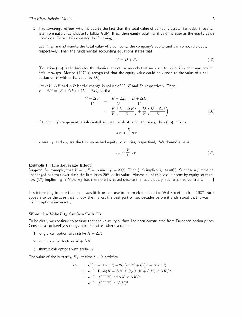
2. The leverage effect which is due to the fact that the total value of company assets, i.e. debt + equity,is a more natural candidate to follow GBM. If so, then equity volatility should increase as the equity valuedecreases. To see this consider the following:

Let V , E and D denote the total value of a company, the company’s equity and the company’s debt,respectively. Then the fundamental accounting equations states that

V = D + E. (15)

(Equation (15) is the basis for the classical structural models that are used to price risky debt and creditdefault swaps. Merton (1970’s) recognized that the equity value could be viewed as the value of a calloption on V with strike equal to D.)

Let ∆V , ∆E and ∆D be the change in values of V , E and D, respectively. ThenV + ∆V = (E + ∆E) + (D + ∆D) so that

V + ∆V

V=

E + ∆E

V+D + ∆D

V

=E

V

(E + ∆E

E

)+D

V

(D + ∆D

D

)(16)

If the equity component is substantial so that the debt is not too risky, then (16) implies

σV ≈E

VσE

where σV and σE are the firm value and equity volatilities, respectively. We therefore have

σE ≈V

EσV . (17)

Example 1 (The Leverage Effect)Suppose, for example, that V = 1, E = .5 and σV = 20%. Then (17) implies σE ≈ 40%. Suppose σV remainsunchanged but that over time the firm loses 20% of its value. Almost all of this loss is borne by equity so thatnow (17) implies σE ≈ 53%. σE has therefore increased despite the fact that σV has remained constant.

It is interesting to note that there was little or no skew in the market before the Wall street crash of 1987. So itappears to be the case that it took the market the best part of two decades before it understood that it waspricing options incorrectly.

What the Volatility Surface Tells Us

To be clear, we continue to assume that the volatility surface has been constructed from European option prices.Consider a butterfly strategy centered at K where you are:

1. long a call option with strike K −∆K

2. long a call with strike K + ∆K

3. short 2 call options with strike K

The value of the butterfly, B0, at time t = 0, satisfies

B0 = C(K −∆K,T )− 2C(K,T ) + C(K + ∆K,T )

≈ e−rT Prob(K −∆K ≤ ST ≤ K + ∆K)×∆K/2

≈ e−rT f(K,T )× 2∆K ×∆K/2

= e−rT f(K,T )× (∆K)2


where f(K,T ) is the (risk-neutral) probability density function (PDF) of ST evaluated at K. We therefore have

f(K,T ) ≈ erTC(K −∆K,T )− 2C(K,T ) + C(K + ∆K,T )

(∆K)2. (18)

Letting ∆K → 0 in (18), we obtain

f(K,T ) = erT∂2C

∂K2.

The volatility surface therefore gives the marginal risk-neutral distribution of the stock price, ST , for any time,T . It tells us nothing about the joint distribution of the stock price at multiple times, T1, . . . , Tn.

This should not be surprising since the volatility surface is constructed from European option prices and thelatter only depend on the marginal distributions of ST .

Example 2 (Same marginals, different joint distributions)Suppose there are two time periods, T1 and T2, of interest and that a non-dividend paying security hasrisk-neutral distributions given by

ST1= e(r−σ2/2)T1+σ

√T1 Z1 (19)

ST2= e

(r−σ2/2)T2+σ√T2

(ρZ1+√

1−ρ2Z2

)(20)

where Z1 and Z2 are independent N(0, 1) random variables. Note that a value of ρ > 0 can capture amomentum effect and a value of ρ < 0 can capture a mean-reversion effect. We are also implicitly assumingthat S0 = 1.

Suppose now that there are two securities, A and B say, with prices S(A)t and S

(B)t given by (19) and (20) at

times t = T1 and t = T2, and with parameters ρ = ρA and ρ = ρB , respectively. Note that the marginal

distribution of S(A)t is identical to the marginal distribution of S

(B)t for t ∈ {T1, T2}. It therefore follows that

options on A and B with the same strike and maturity must have the same price. A and B therefore haveidentical volatility surfaces.

But now consider a knock-in put option with strike 1 and expiration T2. In order to knock-in, the stock price attime T1 must exceed the barrier price of 1.2. The payoff function is then given by

Payoff = max (1− ST2, 0) 1{ST1

≥1.2}.

Question: Would the knock-in put option on A have the same price as the knock-in put option on B?

Question: How does your answer depend on ρA and ρB?

Question: What does this say about the ability of the volatility surface to price barrier options?

3 The Greeks

We now turn to the sensitivities of the option prices to the various parameters. These sensitivities, or theGreeks are usually computed using the Black-Scholes formula, despite the fact that the Black-Scholes model isknown to be a poor approximation to reality. But first we return to put-call parity.

Put-Call Parity

Consider a European call option and a European put option, respectively, each with the same strike, K, andmaturity T . Assuming a continuous dividend yield, q, then put-call parity states

e−rT K + Call Price = e−qT S + Put Price. (21)


This of course follows from a simple arbitrage argument and the fact that both sides of (21) equal max(ST ,K)at time T . Put-call parity is useful for calculating Greeks. For example7, it implies that Vega(Call) = Vega(Put)and that Gamma(Call) = Gamma(Put). It is also extremely useful for calibrating dividends andconstructing the volatility surface.

The Greeks

The principal Greeks for European call options are described below. The Greeks for put options can becalculated in the same manner or via put-call parity.

Definition: The delta of an option is the sensitivity of the option price to a change in the price of theunderlying security.

The delta of a European call option satisfies

delta =∂C

∂S= e−qT Φ(d1).

This is the usual delta corresponding to a volatility surface that is sticky-by-strike. It assumes that as theunderlying security moves, the volatility of the option does not move. If the volatility of the option did movethen the delta would have an additional term of the form vega× ∂σ(K,T )/∂S. In this case we would say thatthe volatility surface was sticky-by-delta. Equity markets typically use the sticky-by-strike approach whencomputing deltas. Foreign exchange markets, on the other hand, tend to use the sticky-by-delta approach.Similar comments apply to gamma as defined below.

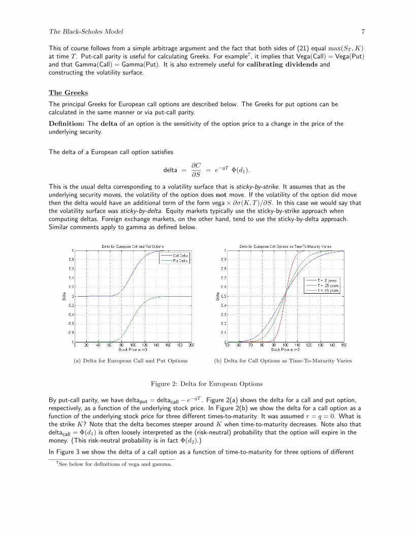
(a) Delta for European Call and Put Options (b) Delta for Call Options as Time-To-Maturity Varies

Figure 2: Delta for European Options

By put-call parity, we have deltaput = deltacall − e−qT . Figure 2(a) shows the delta for a call and put option,respectively, as a function of the underlying stock price. In Figure 2(b) we show the delta for a call option as afunction of the underlying stock price for three different times-to-maturity. It was assumed r = q = 0. What isthe strike K? Note that the delta becomes steeper around K when time-to-maturity decreases. Note also thatdeltacall = Φ(d1) is often loosely interpreted as the (risk-neutral) probability that the option will expire in themoney. (This risk-neutral probability is in fact Φ(d2).)

In Figure 3 we show the delta of a call option as a function of time-to-maturity for three options of different

7See below for definitions of vega and gamma.


Figure 3: Delta for European Call Options as a Function of Time-To-Maturity

money-ness. Are there any surprises here? What would the corresponding plot for put options look like?

Definition: The gamma of an option is the sensitivity of the option’s delta to a change in the price of theunderlying security.

The gamma of a call option satisfies

gamma =∂2C

∂S2= e−qT

φ(d1)

σS√T

where φ(·) is the standard normal PDF.

(a) Gamma as a Function of Stock Price (b) Gamma as a Function of Time-to-Maturity

Figure 4: Gamma for European Options

In Figure 4(a) we show the gamma of a European option as a function of stock price for three differenttime-to-maturities. Note that by put-call parity, the gamma for European call and put options with the samestrike are equal. Gamma is always positive due to option convexity. Traders who are long gamma can makemoney by gamma scalping. Gamma scalping is the process of regularly re-balancing your options portfolio to be


delta-neutral. However, you must pay for this long gamma position up front with the option premium. In Figure4(b), we display gamma as a function of time-to-maturity. Can you explain the behavior of the three curves inFigure 4(b)?

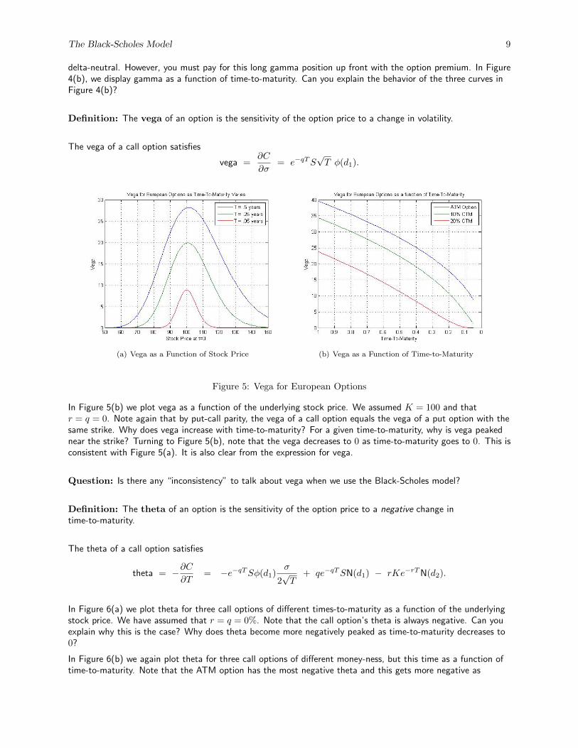
Definition: The vega of an option is the sensitivity of the option price to a change in volatility.

The vega of a call option satisfies

vega =∂C

∂σ= e−qTS

√T φ(d1).

(a) Vega as a Function of Stock Price (b) Vega as a Function of Time-to-Maturity

Figure 5: Vega for European Options

In Figure 5(b) we plot vega as a function of the underlying stock price. We assumed K = 100 and thatr = q = 0. Note again that by put-call parity, the vega of a call option equals the vega of a put option with thesame strike. Why does vega increase with time-to-maturity? For a given time-to-maturity, why is vega peakednear the strike? Turning to Figure 5(b), note that the vega decreases to 0 as time-to-maturity goes to 0. This isconsistent with Figure 5(a). It is also clear from the expression for vega.

Question: Is there any “inconsistency” to talk about vega when we use the Black-Scholes model?

Definition: The theta of an option is the sensitivity of the option price to a negative change intime-to-maturity.

The theta of a call option satisfies

theta = −∂C∂T

= −e−qTSφ(d1)σ

2√T

+ qe−qTSN(d1) − rKe−rTN(d2).

In Figure 6(a) we plot theta for three call options of different times-to-maturity as a function of the underlyingstock price. We have assumed that r = q = 0%. Note that the call option’s theta is always negative. Can youexplain why this is the case? Why does theta become more negatively peaked as time-to-maturity decreases to0?

In Figure 6(b) we again plot theta for three call options of different money-ness, but this time as a function oftime-to-maturity. Note that the ATM option has the most negative theta and this gets more negative as


(a) Theta as a Function of Stock Price (b) Theta as a Function of Time-to-Maturity

Figure 6: Theta for European Options

time-to-maturity goes to 0. Can you explain why?

Options Can Have Positive Theta: In Figure 7 we plot theta for three put options of different money-nessas a function of time-to-maturity. We assume here that q = 0 and r = 10%. Note that theta can be positive forin-the-money put options. Why? We can also obtain positive theta for call options when q is large. In typicalscenarios, however, theta for both call and put options will be negative.

Figure 7: Positive Theta is Possible

Delta-Gamma-Vega Approximations to Option Prices

A simple application of Taylor’s Theorem says

C(S + ∆S, σ + ∆σ) ≈ C(S, σ) + ∆S∂C

∂S+

1

2(∆S)2 ∂

2C

∂S2+ ∆σ

∂C

∂σ

= C(S, σ) + ∆S × δ +1

2(∆S)2 × Γ + ∆σ × vega


where C(S, σ) is the price of a derivative security as a function8 of the current stock price, S, and the impliedvolatility, σ. We therefore obtain

P&L = δ∆S +Γ

2(∆S)2 + vega ∆σ

= delta P&L + gamma P&L + vega P&L

When ∆σ = 0, we obtain the well-known delta-gamma approximation. This approximation is often used, forexample, in historical Value-at-Risk (VaR) calculations for portfolios that include options. We can also write

P&L = δS

(∆S

S

)+

ΓS2

2

(∆S

S

)2

+ vega ∆σ

= ESP× Return + $Gamma× Return2 + vega ∆σ

where ESP denotes the equivalent stock position or “dollar” delta.

4 Delta Hedging

In the Black-Scholes model with GBM, an option can be replicated exactly by delta-hedging the option. Infact the Black-Scholes PDE we derived earlier was obtained by a delta-hedging / replication argument. The ideabehind delta-hedging is to re-balance the portfolio of the option and stock continuously so that you always havea total delta of zero after re-balancing. Of course it is not practical in to hedge continuously and so instead wehedge periodically. Periodic or discrete hedging then results in some replication error.

Let Pt denote the time t value of the discrete-time self-financing strategy that attempts to replicate the optionpayoff and let C0 denote the initial value of the option. The replicating strategy is then given by

P0 := C0 (22)

Pti+1= Pti + (Pti − δtiSti) r∆t + δti

(Sti+1

− Sti + qSti∆t)

(23)

where ∆t := ti+1 − ti is the length of time between re-balancing (assumed constant for all i), r is the annualrisk-free interest rate (assuming per-period compounding), q is the dividend yield and δti is the Black-Scholesdelta at time ti. This delta is a function of Sti and some assumed implied volatility, σimp say. Note that (22)and (23) respect the self-financing condition. Stock prices are simulated assuming St ∼ GBM(µ, σ) so that

St+∆t = Ste(µ−σ2/2)∆t+σ

√∆tZ

where Z ∼ N(0, 1). Note the option implied volatility, σimp, need not equal σ which in turn need not equal therealized volatility (when we hedge periodically as opposed to continuously). This has interesting implications forthe trading P&L which we may define as

P&L := PT − (ST −K)+

in the case of a short position in a call option with strike K and maturity T . Note that PT is the terminal valueof the replicating strategy in (23). Many interesting questions now arise:

Question: If you sell options, what typically happens the total P&L if σ < σimp?

Question: If you sell options, what typically happens the total P&L if σ > σimp?

Question: If σ = σimp what typically happens the total P&L as the number of re-balances increases?

Some Answers to Delta-Hedging Questions

Recall that the price of an option increases as the volatility increases. Therefore if realized volatility is higherthan expected, i.e. the level at which it was sold, we expect to lose money on average when we delta-hedge an

8The price may also depend on other parameters, in particular time-to-maturity, but we suppress that dependence here.


option that we sold. Similarly, we expect to make money when we delta-hedge if the realized volatility is lowerthan the level at which it was sold.

In general, however, the payoff from delta-hedging an option is path-dependent, i.e. it depends on the pricepath taken by the stock over the entire time interval. In fact, we can show that the payoff from continuouslydelta-hedging an option satisfies

P&L =

∫ T

0

S2t

2

∂2Vt∂S2

(σ2imp − σ2

t

)dt (24)

where Vt is the time t value of the option and σt is the realized instantaneous volatility at time t.

The termS2t

2∂2Vt

∂S2 is often called the dollar gamma, as discussed earlier. It is always positive for a call or putoption, but it goes to zero as the option moves significantly into or out of the money.

Returning to self-financing trading strategy of (22) and (23), note that we can choose any model we like for thesecurity price dynamics. In particular, we are not restricted to choosing geometric Brownian motion and otherdiffusion or jump-diffusion models could be used instead. It is interesting to simulate these alternative modelsand to then observe what happens to the replication error in (24) where the δti ’s are computed assuming(incorrectly) a geometric Brownian motion price dynamics.

the black-scholes model - columbia universitymh2078/foundationsfe/blackscholes.pdf · 2 the...

Documents