U.U.D.M. Project Report 2013:8

Examensarbete i matematik, 15 hpHandledare och examinator: Johan TyskMaj 2013

The Black-Scholes Equation and Formula

Olle Karlsson

Department of MathematicsUppsala University

Abstract

The purpose of this paper is to present fundamental arbitrage theory and itsapplications to pricing financial derivatives, in a way that does not requirea previous knowledge of Stochastic Calculus or Measure theory. It starts offwith an easy introduction to the financial market in Chapter 1 and tacklesthe tough tools, namely Stochastic calculus, in Chapter 2. We use thistheory to derive the Black-Scholes equation and Black-Scholes formula.

Contents

1 The Market 3

2 Stochastic Calculus 62.1 The Ito Integral . . . . . . . . . . . . . . . . . . . . . . . . . . 62.2 Ito’s Lemma . . . . . . . . . . . . . . . . . . . . . . . . . . . . 102.3 Stochastic Differential Equations . . . . . . . . . . . . . . . . 13

3 The Black-Scholes Model 153.1 Feynman-Kac . . . . . . . . . . . . . . . . . . . . . . . . . . . 183.2 Black-Scholes formula . . . . . . . . . . . . . . . . . . . . . . 20

2

Chapter 1

The Market

If you believe that the stock Eriksson B in six months would increase by 40percent, what would you be willing to pay for a contract saying that in sixmonths you can buy it for the same price as today?

In 1973 Fischer Black and Myron Scholes published the paper ”ThePricing of Options and Corporate Liabilities” in the Journal of PoliticalEconomy, see [3]. It contains an equation which was going to become famousbecause it did something new. It describe how to create a risk free portfolioand also gave the explicit price for this portfolio. The real market is toocomplex to be modelled in its entirety so the models used were simplified,and thus did not give exact predictions on the real market.

Since then many papers have been published expanding the model. Oftenobjects in the aforementioned model are extrapolated from the market andnot always given a proper definition, for the reader unfamiliar with themarket we will define the objects needed to develop an understanding of themodel.

First when inspecting a financial market the most prominent objects arefinancial derivatives and assets. Financial derivatives is a broad categorisa-tion of objects that are traded on a market and whose values are derivedfrom some underlying assets.

Definition 1. A financial derivative is an object on the market that can bebought or sold and is dependent on one or more assets.

It follows from the definition that an asset is also a financial derivativealthough they are not usually classified as such. Some specific financialderivatives will be defined and used extensively later on. It is important tounderstand the assumptions going into developing the model, some of whichwe will introduce now.

Assumptions 1. These assumptions explains how trading in the modelworks, since the model is an idealization of the real market.

3

• Short positions (negative financial derivatives) and fractional holdingsare allowed.

• There is no cost for selling or buying assets or derivatives.

• The buying price is the same as the selling price.

• The market is liquid meaning it is always possible to buy and/or sellunlimited quantities on the market.

Important assets are: A stock, it’s an asset and modelled by a stochasticprocess.A bond, is a risk-free asset modelled by a deterministic process with rate ofreturn r(t).

Note that bonds adds the possibility to borrow unlimited amounts byselling bonds short. A portfolio h is a collection of some stocks and bonds.A portfolio can be self-financing meaning there is no money put into theportfolio and all buying of new assets must be financed with the selling ofother assets, this will be defined rigorous in Chapter 3. Other objects onthe market, more often classified as financial derivatives are options, futuresand forwards. In this paper we will only work with options.

Definition 2. An option is a contract that gives the owner the right (butnot the obligation) to buy or sell a derivative at a specified price called astriking price on or before a striking time T .

Important options include European Put/Call options and AmericanPut/Call options. These are the most common types of options. In thispaper we will explore the European Call option.

Definition 3. A European put/call option is an option to sell/buy a deriva-tive at the exact time T .

In contrary to a European option an American option can be exercisedanytime between when the option is bought and time T. For a portfolioh we need something to track the value of that portfolio, we call that thevalue process V (t, h). This makes it possible to define the most importantassumption about the market, that the market is efficient, meaning it is freeof arbitrage. This is a very basic condition, saying that it is not possible tomake a risk-free profit.

Definition 4. An arbitrage possibility on the market is a self-financed port-folio h such that:

1. V (0, h) = 0.

2. P (V (T, h) ≥ 0) = 1.

4

3. P (V (T, h) > 0) > 0.

The market is arbitrage free if and only if there are no arbitrage possibilities.

Now to the question posed in the beginning.

Example 1. If you believe that the stock Eriksson B in six months wouldincrease by 40 percent, what would you be willing to pay for a contract sayingthat in six months you can buy it for the same price as today?

Today Eriksson B is say 80SEK.Then this clearly is a European call option with strike price 80SEK and

expiration date 6 months from now.

5

Chapter 2

Stochastic Calculus

This chapter will be devoted to the development of stochastic calculus. Itis as the name suggests the calculus of stochastic processes and was firstdeveloped to determine rocket trajectories.Recall that a stochastic process in continuous time is some function

X : R× Ω −→ R

where Ω is some probability space.

2.1 The Ito Integral

In this section we develop the stochastic integral and we begin by defininga special process that will be important. The presentation is based on [1].

Definition 5. A stochastic process X is called a Wiener process, denotedW, if the following conditions hold.

1. W (0) = 0.

2. The process has independent increments, i.e. if r < s ≤ t < u thenW (u)−W (t) and W (s)−W (r) are independent stochastic variables.We will often use ∆W to denote such independent increments.

3. For s < t the stochastic variable W (t)−W (s) has the Normal distri-bution N [0, t− s].

4. W has continuous trajectories.

For the coming argument we will fix ω ∈ Ω making

X : R× Ω −→ R

becomeX : R× ω −→ R

6

with ω being unknown. To be able to continue we need a definition frommeasure theory. But since measure theory is outside the scoop of this paperit will be introduced in a heuristic way. For the reader well acquainted withmeasure theory the definition is the needed sigma algebra. This is neededso that parts of ω can be considered known, ω can be viewed as the infinitesequence of coin tosses and the following definition makes it possible to knowa subsequence.

Definition 6. The symbol FXt denotes “the information generated by Xon the interval [0, t]”. or alternatively “what has happened to X over theinterval [0, t]”. If, based upon observations of the trajectory X(s); 0 ≤ s ≤t, it is possible to decide whether a given event A has occurred or not, wewrite this as

A ∈ FXtor say that “A is FXt -measurable”. If the value of a given stochastic vari-able Z can be completely determined given observations of the trajectoryX(s); 0 ≤ s ≤ t, then we also write

Z ∈ FXt .

If Y is a stochastic process such that we have

Y (t) ∈ FXt

for all t ≥ 0 then we say that Y is adapted to the filtration FXt t≥0.

To guarantee that a process can be integrated in a meaningful way weneed to impose some restrictions.

Definition 7. 1. We say that the process g belongs to the class £2[a, b]if the following conditions are satisfied:

•∫ ba E[g2(s)]ds <∞.

• The process g is adapted to the FWt -filtration.

2. We say that the process g belong to the class £2 if g ∈ £2[0, t] for allt > 0.

An important observation, although not at all trivial is that for anyprocess g

g ∈ £2[a, b]⇒ g ∈ L2[a, b] for any fixed ω ∈ Ω.

To prove this measure theory is needed (The Fubini Theorem) so it will

not be done here. Now we begin defining the stochastic integral∫ ba g(s)dW (s)

for g ∈ £2[a, b]. First suppose that g is simple, then there exist deterministic

7

points in time a = t0 < t1 < ... < tn = b such that g is constant on eachsubinterval. This makes it natural to define the integral by

b∫a

g(s)dW (s) =n−1∑k=0

g(tk)[W (tk+1)−W (tk)].

For a general process g ∈ £2[a, b] we approximate it with a sequence of

simple processes gn∞1 such thatb∫aE[(gn(s)− g(s))2]ds −→ 0 as n −→∞.

Since L2[a, b] is complete (every Cauchy sequence converges) the integralb∫agn(s)dW (s) converges to something in L2[a, b], and we let

b∫a

g(s)dW (s) = limn→∞

b∫a

gn(s)dW (s).

There are some important properties of this integral.

Theorem 1. Let g be a process such that g is adapted to the FWt -filtrationand

b∫a

E[g2(s)

]ds <∞.

Then the following holds

E

b∫a

g(s)dW (s)

= 0,

and

E

b∫a

g(s)dW (s)

2 =

b∫a

E[g2(s)

]ds.

Proof. The first part is pretty straight forward, giving

E

b∫a

g(s)dW (s)

= E

[limn→∞

n−1∑k=0

gn(tk) (W (tk+1)−W (tk))

]=

= limn→∞

n−1∑k=0

E [gn(tk)]E [W (tk+1)−W (tk)] = 0.

This holds since g(tk) is adapted to the filtration, meaning that it is onlydependent on the behaviour of the wiener process on the interval [0, tk].

8

Since the Wiener increment is a forward increment dependent only on theinterval [tk, tk+1], the Wiener increment and g(tk) are independent. Last theexpected values of the increments are 0.

Next we have

E

b∫a

g(s)dW (s)

2 = V ar

b∫a

g(s)dW (s)

=

= V ar

[limn→∞

n−1∑k=0

gn(tk) (W (tk+1)−W (tk))

].

It can be shown that these stochastic variables are uncorrelated giving

limn→∞

n−1∑k=0

V ar [gn(tk) (W (tk+1)−W (tk))] .

We have already argued that the increment and gn(tk) are independent,giving us

limn→∞

n−1∑k=0

(E[gn(tk)]

2V ar[W (tk+1)−W (tk)]+

+E[W (tk+1)−W (tk)]2V ar[gn(tk)]+

+V ar[W (tk+1)−W (tk)]V ar[gn(tk)]

).

V ar[W (tk+1)−W (tk)] = tk+1 − tk and so

limn→∞

n−1∑k=0

(E[gn(tk)]

2 (tk+1 − tk) + V ar[gn(tk)] (tk+1 − tk)).

Taking the limit we get, by the Riemann-Stiltjes Integral

b∫a

E[g(t)]2 + V ar[g(t)]dt.

The identity V ar[X] = E[X2]− E[X]2 completes the proof giving

b∫a

E[g(t)]2 + E[g2(t)]− E[g(t)]2dt =

b∫a

E[g2(t)]dt.

9

2.2 Ito’s Lemma

Now we present one of the most important results in Stochastic calculus. Itwas first stated, boldly, by Ito in one of his papers as a lemma.Let X be a stochastic process and suppose that there exist some a ∈ R andµ(t), σ(t) ∈ FXt t≥0 such that the following hold for all t ≥ 0

X(t) = a+

t∫0

µ(s)ds+

t∫0

σ(s)dW (s).

Further assume that we have a C2-function

f : R+ ×R −→ R

and define a new process Z by

Z(t) = f(t,X(t)).

The arguments of the function has been omitted in favour for readability.

Theorem 2 (Ito’s Lemma). Assume that the process X satisfies the integralequation above and Z is defined as above. Then Z satisfies the followingintegral equation

Z(t) = Z(0) +

t∫0

(∂f

∂t+ µ

∂f

∂X+

1

2σ2

∂2f

∂X2

)ds+

t∫0

σ∂f

∂XdW.

Proof. This proof is based on the sketches in [1] and [2] First we divide theinterval [0, t] into n equal subintervals such that 0 = t0 < t1 < ... < tn = t.Then

f(t,X(t))− f(0, X(0)) =n−1∑k=0

(f(tk+1, X(tk+1))− f(tk, X(tk)) .

Using Taylor’s theorem we get

f(tk+1, X(tk+1))− f(tk, X(tk)) =∂f(tk, X(tk))

∂t∆t+

∂f(tk, X(tk))

∂X∆Xk+

1

2

∂2f(tk, X(tk))

∂t2∆t2 +

∂2f(tk, X(tk))

∂t∂X∆t∆Xk +

1

2

∂2f(tk, X(tk))

∂X2(∆Xk)

2 +Qk

where Qk is the remainder and ∆t = tn = tk+1 − tk. Also since µ and σ

are adapted to the filtration there is a n big enough such that

∆Xk = X(tk+1)−X(tk) =

10

=

tk+1∫tk

µ(s)ds+

tk+1∫tk

σ(s)dW (s) = µ(tk)∆t+ σ(tk)∆Wk.

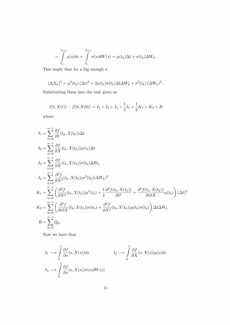
This imply that for a big enough n

(∆Xk)2 = µ2(tk) (∆t)2 + 2µ(tk)σ(tk)∆t∆Wk + σ2(tk) (∆Wk)

2 .

Substituting these into the sum gives us

f(t,X(t))− f(0, X(0)) = I1 + I2 + I3 +1

2I4 +

1

2K1 +K2 +R

where

I1 =

n−1∑k=0

∂f

∂t(tk, X(tk))∆t

I2 =n−1∑k=0

∂f

∂X(tk, X(tk))µ(tk)∆t

I3 =n−1∑k=0

∂f

∂X(tk, X(tk))σ(tk)∆Wk

I4 =

n−1∑k=0

∂2f

∂X2(tk, X(tk))σ

2(tk)(∆Wk)2

K1 =n−1∑k=0

(∂2f

∂X2(tk, X(tk))µ

2(tk) +1

2

∂2f(tk, X(tk))

∂t2+∂2f(tk, X(tk))

∂t∂Xµ(tk)

)(∆t)2

K2 =

n−1∑k=0

(∂2f

∂t∂X(tk, X(tk))σ(tk) +

∂2f

∂X2(tk, X(tk))µ(tk)σ(tk)

)∆t∆Wk

R =

n−1∑k=0

Qk.

Now we have that

I1 −→t∫

0

∂f

∂s(s,X(s))ds I2 −→

t∫0

∂f

∂X(s,X(s))µ(s)ds

I3 −→t∫

0

∂f

∂x(s,X(s))σ(s)dW (s)

11

by definition as n→∞.

I4 −→t∫

0

∂2f

∂X2(s,X(s))σ2(s)ds

is shown by naming ∂2f∂X2 (tk, X(tk))σ

2(tk) = ak and evaluating

E

(n−1∑k=0

ak(∆Wk)2 −

n−1∑k=0

ak∆t

)2 = E

(n−1∑k=0

ak((∆Wk)

2 −∆t))2

=

E

n−1∑k=0

a2k((∆Wk)

2 −∆t)2

+ 2∑k 6=l

akal((∆Wk)

2 −∆t) (

(∆Wl)2 −∆t

) .ak, al, (∆Wk)

2 −∆t and (∆Wl)2 −∆t are all independent, making the

second sum disappear.

E

[n−1∑k=0

a2k((∆Wk)

2 −∆t)2]

=n−1∑k=0

E[a2k((∆Wk)

4 − 2∆t(∆Wk)2 + ∆t2

)]=

n−1∑k=0

E[a2k] (

3∆t2 − 2∆t2 + ∆t2)

= 2

n−1∑k=0

E[a2k]

∆t2 → 0

by the coming argument. Proving that the sum converge in probabil-

ity to the integral. For K1 we call ∂2f∂X2 (tk, X(tk))µ

2(tk) + 12∂2f(tk,X(tk))

∂t2+

∂2f(tk,X(tk))∂t∂X µ(tk) = a(tk) and use that a(t) is bounded( everything in a(t)

can be approximated with bounded functions).

|K1| ≤n−1∑k=0

|a(tk)(∆t)2|

≤ sups∈[0,t]

|a(s)|n−1∑k=0

|(∆t)2|

= sups∈[0,t]

|a(s)||n(t

n

)2

|

which goes to 0 as n→∞.

K2 is similar to I4 with ak = ∂2f∂t∂X (tk, X(tk))σ(tk)+

∂2f∂X2 (tk, X(tk))µ(tk)σ(tk)

12

E

(n−1∑k=0

ak∆t∆Wk

)2 =

n−1∑k=0

E[(ak)

2]E[∆W 2

k

]∆t =

n−1∑k=0

E[(ak)

2]

∆t3 → 0.

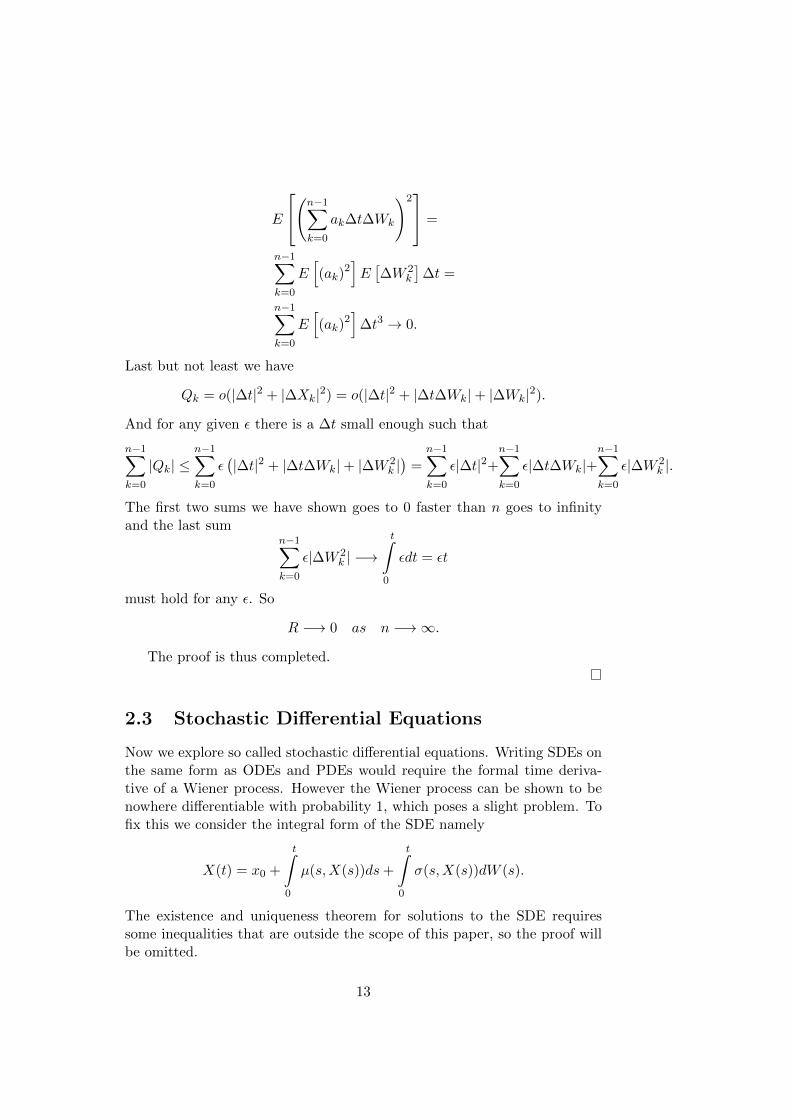
Last but not least we have

Qk = o(|∆t|2 + |∆Xk|2) = o(|∆t|2 + |∆t∆Wk|+ |∆Wk|2).

And for any given ε there is a ∆t small enough such that

n−1∑k=0

|Qk| ≤n−1∑k=0

ε(|∆t|2 + |∆t∆Wk|+ |∆W 2

k |)

=n−1∑k=0

ε|∆t|2+n−1∑k=0

ε|∆t∆Wk|+n−1∑k=0

ε|∆W 2k |.

The first two sums we have shown goes to 0 faster than n goes to infinityand the last sum

n−1∑k=0

ε|∆W 2k | −→

t∫0

εdt = εt

must hold for any ε. So

R −→ 0 as n −→∞.

The proof is thus completed.

2.3 Stochastic Differential Equations

Now we explore so called stochastic differential equations. Writing SDEs onthe same form as ODEs and PDEs would require the formal time deriva-tive of a Wiener process. However the Wiener process can be shown to benowhere differentiable with probability 1, which poses a slight problem. Tofix this we consider the integral form of the SDE namely

X(t) = x0 +

t∫0

µ(s,X(s))ds+

t∫0

σ(s,X(s))dW (s).

The existence and uniqueness theorem for solutions to the SDE requiressome inequalities that are outside the scope of this paper, so the proof willbe omitted.

13

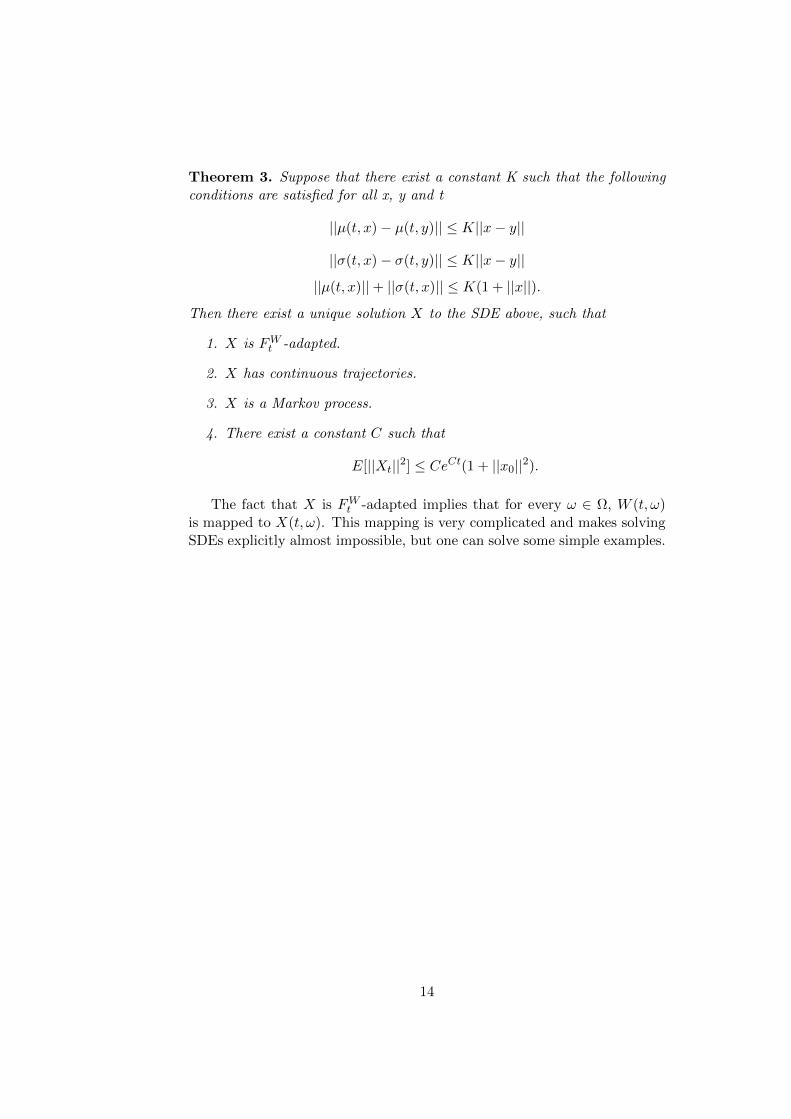
Theorem 3. Suppose that there exist a constant K such that the followingconditions are satisfied for all x, y and t

||µ(t, x)− µ(t, y)|| ≤ K||x− y||

||σ(t, x)− σ(t, y)|| ≤ K||x− y||

||µ(t, x)||+ ||σ(t, x)|| ≤ K(1 + ||x||).

Then there exist a unique solution X to the SDE above, such that

1. X is FWt -adapted.

2. X has continuous trajectories.

3. X is a Markov process.

4. There exist a constant C such that

E[||Xt||2] ≤ CeCt(1 + ||x0||2).

The fact that X is FWt -adapted implies that for every ω ∈ Ω, W (t, ω)is mapped to X(t, ω). This mapping is very complicated and makes solvingSDEs explicitly almost impossible, but one can solve some simple examples.

14

Chapter 3

The Black-Scholes Model

Now we have the tools needed to develop the Black-Scholes model. Themain reference is [1].

Definition 8. Consider a financial market with vector price process S (thisis the vector with all assets). A contingent claim with date of maturity

(exercise date) T , also called a T -claim, is any stochastic variable χ ∈ F ST .

A contingent claim χ is called a simple claim if it is of the form

χ = Φ(

S (T )).

The function Φ is called the contract function.

From this point onwards we will only consider simple claims. On themarket a claim is a contract that depends on S and the main problem isto determine a fair price on the claim (if it exist). Π(t, χ) is the priceprocess of the claim χ. For t = T , χ is known and the price is exactly χ soΠ(T, χ) = χ. For t < T , Π(t, χ) is unknown. Given N assets with valuesZ1(t), ..., ZN (t) at time t a trading strategy is a N-dimensional stochasticprocess (a1(t), ..., aN (t)) that represent the allocations into the assets attime t. Then at time t we have

V (t, h) =

N∑n=1

an(t)Zn(t).

Now we can give the self-financing criteria in a formal statement.

Definition 9. A portfolio is called self-financing if the value process V (t, h)satisfies the condition

V (t, h) =

N∑n=1

t∫0

an(s)dZn(t).

15

Lemma 1. The rate of interest in an arbitrage free model must be unique.

Proof. We denote the rate of interest r and suppose there exist some riskfree derivative with return c. If c < r then arbitrage can be achieved byselling the derivative short and buy bonds. If c > r then arbitrage can beachieved by selling bonds short and buy the derivative. So for the model tobe arbitrage free we must have c = r.

We need some more assumptions that we could not include earlier sincethey are a bit technical.

Assumptions 2. We assume that

1. The derivative instrument in question can be bought and sold on amarket.

2. The market is free of arbitrage.

3. The price process for the derivative asset is of the form

Π(t, χ) = F (t, S(t))

where F is some smooth function.

The last assumption, specific to the Black-Scholes model, is that themarket consist of two assets satisfying

B(t) =

t∫0

r ·B(s)ds

S(t) =

t∫0

S(s)µ(s, S(s))ds+

t∫0

S(s)σ(s, S(s))dW (s).

Where B(t) is a riskfree asset with deterministic constant rate of interestr. By the assumption we have Π(t,Φ(S(T ))) = F (t, S(t)), so by the Itoformula we get

Π(t,Φ(S(T ))) = F (0, S(0))+

t∫0

(∂F

∂s+ Sµ

∂F

∂S+

1

2S2σ2

∂2F

∂2S

)ds+

+

t∫0

Sσ∂F

∂SdW.

16

Let us consider a self-financing portfolio consisting of the underlyingstock and bond. To get the right proportions we use the trading strategy(α(t), β(t)) to form the replicating portfolio F (t, S(t)) = α(t)S(t)+β(t)B(t).The self financing assumption implies that

F (t, S(t)) = F (0, S(0)) +

t∫0

α(s)dS(s) +

t∫0

β(s)dB(s) =

= F (0, S(0)) +

t∫0

α(s)µ(s)S(s)ds+

t∫0

α(s)σ(s)S(s)dW (s) +

t∫0

β(s)rB(s)ds.

Since Π(t,Φ(S(T ))) = F (t, S(t)) we get

t∫0

(∂F

∂s+ Sµ

∂F

∂S+

1

2S2σ2

∂2F

∂2S

)ds+

t∫0

Sσ∂F

∂SdW =

=

t∫0

α(s)µ(s)S(s)ds+

t∫0

α(s)σ(s)S(s)dW (s) +

t∫0

β(s)rB(s)dt.

Collecting integrals we get

t∫0

(∂F

∂s+ Sµ

∂F

∂S+

1

2S2σ2

∂2F

∂S2− αµS − βrB

)ds+

+

t∫0

(Sσ

∂F

∂S− Sσα

)dW = 0.

Now we see that if we let α = ∂F∂S the Stochastic integral becomes 0 and we

have a risk-free portfolio. Then we get

t∫0

(∂F

∂s+

1

2σ2S2∂

2F

∂S2+ βrB

)dt = 0.

It is evident that this choice of portfolio also removes the µ process fromthe integral equation. This is the ground breaking discovery made by Blackand Scholes. Since µ is almost impossible to estimate, the discovery that it isnot needed to price certain portfolios was the birth of financial mathematics.

From the strategy equation F (t) = β(t)B(t) + α(t)S(t) we get that

B(t) = F (t)−α(t)S(t)β(t) . Substituting this into the equation give us

t∫0

(∂F

∂s+

1

2σ2S2∂

2F

∂S2+ rS

∂F

∂S− rF

)ds = 0.

17

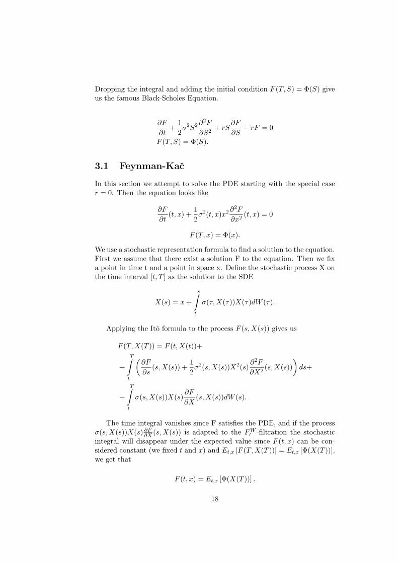
Dropping the integral and adding the initial condition F (T, S) = Φ(S) giveus the famous Black-Scholes Equation.

∂F

∂t+

1

2σ2S2∂

2F

∂S2+ rS

∂F

∂S− rF = 0

F (T, S) = Φ(S).

3.1 Feynman-Kac

In this section we attempt to solve the PDE starting with the special caser = 0. Then the equation looks like

∂F

∂t(t, x) +

1

2σ2(t, x)x2

∂2F

∂x2(t, x) = 0

F (T, x) = Φ(x).

We use a stochastic representation formula to find a solution to the equation.First we assume that there exist a solution F to the equation. Then we fixa point in time t and a point in space x. Define the stochastic process X onthe time interval [t, T ] as the solution to the SDE

X(s) = x+

s∫t

σ(τ,X(τ))X(τ)dW (τ).

Applying the Ito formula to the process F (s,X(s)) gives us

F (T,X(T )) = F (t,X(t))+

+

T∫t

(∂F

∂s(s,X(s)) +

1

2σ2(s,X(s))X2(s)

∂2F

∂X2(s,X(s))

)ds+

+

T∫t

σ(s,X(s))X(s)∂F

∂X(s,X(s))dW (s).

The time integral vanishes since F satisfies the PDE, and if the processσ(s,X(s))X(s) ∂F∂X (s,X(s)) is adapted to the FWt -filtration the stochasticintegral will disappear under the expected value since F (t, x) can be con-sidered constant (we fixed t and x) and Et,x [F (T,X(T ))] = Et,x [Φ(X(T ))],we get that

F (t, x) = Et,x [Φ(X(T ))] .

18

Let r ∈ R. Then we have the equation

∂F

∂t(t, x) +

1

2σ2(t, x)x2

∂2F

∂x2(t, x) + rx

∂F

∂x(t, x)− rF (t, x) = 0

F (T, x) = Φ(x).

Consider the function G(t, x) = e−rtF (t, x). Multiply the equation withe−rt and use G(t, x) to rewrite it as

∂G

∂t(t, x) +

1

2σ2(t, x)x2

∂2G

∂x2(t, x) + r

∂G

∂x(t, x) = 0

G(T, x) = Φ(x)ert.

This is similar to what we had before. However there is another term inthe equation. This problem can be fixed by changing the SDE previouslydefined to be

X(s) = x+

s∫t

σ(τ,X(τ))X(τ)dW (τ).

For r ∈ R we instead define X(s) as

X(s) = x+

s∫t

rX(τ)dτ +

s∫t

σ(τ,X(τ))X(τ)dW (τ).

This will make sure that the time integral in the Ito formula disappears.

Also if the process σ(s,X(s))X(s) ∂G∂X (s,X(s)) is adapted to the FWt -filtration the stochastic integral will disappear under the expected value.

We get

G(t, x) = Et,x[Φ(X(T ))erT

].

Changing back to F (t, x) and moving some exponents around we get theFeynman-Kac stochastic representation formula

F (t, x) = e−r(T−t)Et,x [Φ(X(T ))] .

This is an explicit pricing formula for certain derivatives, it certainly hasits limitations but is used extensively by traders to evaluate a fair price on,for example, European Call Options. The Feynman-Kac stochastic represen-tation formula can be evaluated numerically with for example a Monte-Carlomethod. Another way to numerically evaluate the function would be directlyfrom the PDE with possibly a finite difference method.

19

3.2 Black-Scholes formula

The SDE

X(s) = x+

s∫t

rX(τ)dτ +

s∫t

σ(τ,X(τ))X(τ)dW (τ)

is very special and can be explicitly solved. Consider the function f(x) =ln(x) and the SDE above, then by the Ito formula we get

ln(X(t)) = ln(x) +

s∫t

r − 1

2σ2(τ,X(τ))dτ +

s∫t

σ(τ,X(τ))dW (τ)

X(t) = x · exp

s∫t

r − 1

2σ2(τ,X(τ))dτ +

s∫t

σ(τ,X(τ))dW (τ)

.When σ is constant this yields the nice expression

X(t) = x · exp

((r − 1

2σ2)

(s− t) + σ(W (s)−W (t))

)Y =

(r − 1

2σ2)

(s − t) + σ(W (s) −W (t)) can be viewed as a normallydistributed stochastic variable.

The Feynman-Kac formula for such processes can be writen as

F (t, s) = e−r(T−t)∞∫−∞

Φ(xey)f(y)dy

where f is the density function for the stochastic variable Y .

For an arbitrary contract function Φ this integral can not be solvedexplicitly, so we will solve it for a European call option where

Φ(x) = max[x−K, 0],

K is the striking price of the contract. Normalizing Y and using the stan-darized normal variable Z the integral becomes

∞∫−∞

max[xe(r−

12σ2)(T−t)+σ

√T−tz −K, 0

]φ(z)dz

where φ is the density of the N [0, 1] distribution.

20

The integrand is 0 when z < z0

z0 =ln(Kx

)−(r − 1

2σ2)

(T − t)σ√T − t

.

∞∫z0

(xe(r−

12σ2)(T−t)+σ

√T−tz −K

)φ(z)dz

=

∞∫z0

xe(r−12σ2)(T−t)+σ

√T−tzφ(z)dz −

∞∫z0

Kφ(z)dz.

The second integral is obviously K · P (Z ≥ z0) = K · P (Z ≤ −z0), thesymmetry in the normal distribution is responsible for the change of inequal-ity. In the first integral we write out the density function and complete thesquare.

∞∫z0

xe(r−12σ2)(T−t)+σ

√T−tzφ(z)dz

=xe(r−

12σ2)(T−t)√

2π

∞∫z0

eσ√T−tz− z2

2 dz

=xer(T−t)√

2π

∞∫z0

e−12(z−σ

√T−t)

2

dz.

We recognize the integral as the density of the N [σ√T − t, 1] distribu-

tion.

xer(T−t)√2π

∞∫z0

e−12(z−σ

√T−t)

2

dz

= xer(T−t) · P (Z − σ√T − t ≥ z0) = xer(T−t) · P (Z ≤ −z0 + σ

√T − t).

That completes the famous Black-Scholes formula.

Theorem 4. The price of a European call option with strike price K andtime of maturity T is given by Π(t) = F (t, S(t)), where

F (t, s) = sP (Z ≤ −z0 + σ√T − t)− e−r(T−t)P (Z ≤ −z0).

Here Z is N(0, 1) distributed and z0 =ln(K

s )−(r− 12σ2)(T−t)

σ√T−t .

21

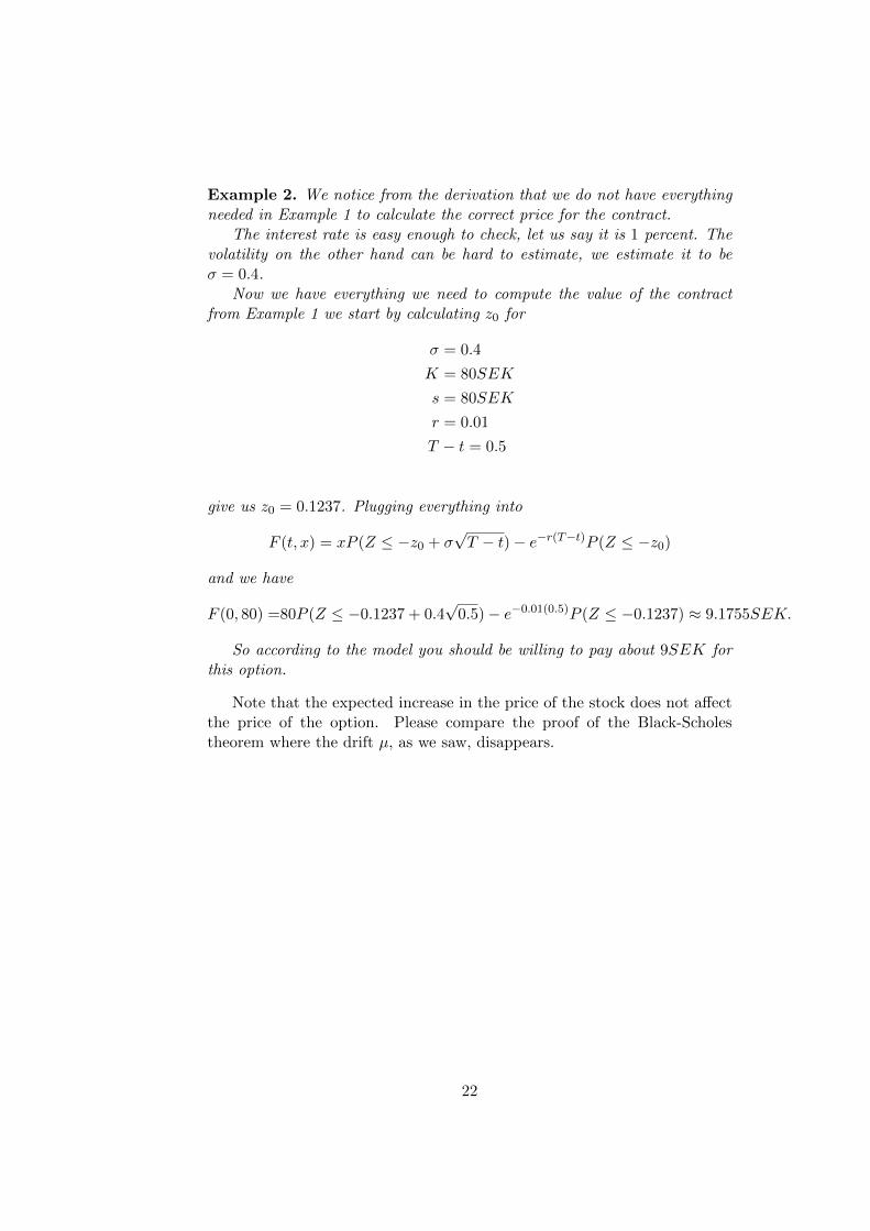
Example 2. We notice from the derivation that we do not have everythingneeded in Example 1 to calculate the correct price for the contract.

The interest rate is easy enough to check, let us say it is 1 percent. Thevolatility on the other hand can be hard to estimate, we estimate it to beσ = 0.4.

Now we have everything we need to compute the value of the contractfrom Example 1 we start by calculating z0 for

σ = 0.4

K = 80SEK

s = 80SEK

r = 0.01

T − t = 0.5

give us z0 = 0.1237. Plugging everything into

F (t, x) = xP (Z ≤ −z0 + σ√T − t)− e−r(T−t)P (Z ≤ −z0)

and we have

F (0, 80) =80P (Z ≤ −0.1237 + 0.4√

0.5)− e−0.01(0.5)P (Z ≤ −0.1237) ≈ 9.1755SEK.

So according to the model you should be willing to pay about 9SEK forthis option.

Note that the expected increase in the price of the stock does not affectthe price of the option. Please compare the proof of the Black-Scholestheorem where the drift µ, as we saw, disappears.

22

Bibliography

[1] Tomas Bjork, Arbitrage Theory in Continuous Time. Oxford UniversityPress Inc, New York, 3rd Edition, 2009.

[2] Bernt Øksendal, Stochastic Differential Equations, An Introduction withApplications. Springer-Verlag, Berlin, 5th Edition, 1998.

[3] Fisher Black and Myron Scholes, The Pricing of Options and CorporateLiabilities. The Journal of Political Economy, Vol. 81, No. 3, 1973, p.637-654.

23