Generalised Fractional-Black-Scholes

Equation: pricing and hedging

Alvaro Cartea

Birkbeck College, University of London

April 2004

Outline

• Levy processes

• Fractional calculus

• Fractional-Black-Scholes

1

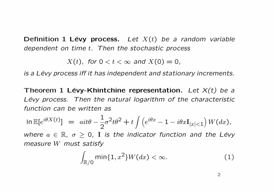
Definition 1 Levy process. Let X(t) be a random variable

dependent on time t. Then the stochastic process

X(t), for 0 < t < ∞ and X(0) = 0,

is a Levy process iff it has independent and stationary increments.

Theorem 1 Levy-Khintchine representation. Let X(t) be a

Levy process. Then the natural logarithm of the characteristic

function can be written as

lnE[eiθX(t)] = aitθ − 1

2σ2tθ2 + t

∫ (eiθx − 1− iθxI|x|<1

)W (dx),

where a ∈ R, σ ≥ 0, I is the indicator function and the Levy

measure W must satisfy∫

R/0min{1, x2}W (dx) < ∞. (1)

2

Which Levy process? Why?

• Brownian motion; Bachelier.

• α-Stable or Levy Stable; Mandelbrot.

• Jump Diffusion; Merton.

• GIG and Generalised Hyperbolic Distribution; Barndorff-Nielsen.

• Variance Gamma; Madan et al.

3

• CGMY, Carr et al.

• KoBol, Tempered Stable; Koponen.

• FMLS; Carr and Wu.

• others.

When specifying a particular Levy process we are basically asking

how do we want to specify the ‘behaviour’ of the jumps, in other

words how is the Levy density w(x) (ie W (dx) = w(x)dx) chosen.

For example

• Size and sign of jumps

• Frequency of jumps

• Existence of moments

• Simplicity

The CGMY process

A simple answer is then to consider a Levy density of the form

wCGMY (x) =

{C|x|−1−Y e−G|x| for x < 0,

Cx−1−Y e−Mx for x > 0,

and the log of the characteristic function is given by

ΨCGMY (θ) = tCΓ(Y ){(M − iθ)Y −MY + (G + iθ)Y −GY }.Here C > 0, G ≥ 0, M ≥ 0 and Y < 2.

4

The Damped-Levy process

wDL(x) =

{Cq |x|−1−α e−λ|x| for x < 0,Cpx−1−αe−λx for x > 0,

and the natural logarithm of the characteristic equation is given

by

ΨDL(θ) = tκα{p(λ− iθ)α + q(λ + iθ)α − λα − iθαλα−1(q − p)

},

for 1 < α ≤ 2 and p + q = 1.

5

The Levy-Stable process

Is a pure jump process with Levy density

wLS(x) =

{Cq |x|−1−α for x < 0,Cpx−1−α for x > 0,

Hence the log of the characteristic function is Ψ(θ) ={ −κα|θ|α {1− iβ sign(θ) tan(απ/2)} for α 6= 1,

−κ|θ|{1 + 2iβ

π sign(θ) ln |θ|}

for α = 1,

here C > 0 is a scale constant, p ≥ 0 and q ≥ 0, with p + q = 1

and β = p− q is the skewness parameter.

6

Fractional Integrals

For an n-fold integral there is the well known formula∫ x

a

∫ x

a· · ·

∫ x

af(x)dx =

1

(n− 1)!

∫ x

a(x− t)n−1f(t)dt.

Note that since (n − 1)! = Γ(n) the expression above may have

a meaning for non-integer values of n.

Definition 2 The Riemann-Liouville Fractional Integral. The

fractional integral of order α > 0 of a function f(x) is given by

D−αa+ f(x) =

1

Γ(α)

∫ x

a(x− ξ)α−1f(ξ)dξ,

and

D−αb− f(x) =

1

Γ(α)

∫ b

x(ξ − x)α−1f(ξ)dξ.

7

Definition 3 The Riemann-Liouville Fractional Derivative.

Dαa+f(x) =

1

Γ(n− α)

dn

dxn

∫ x

a(x− ξ)n−α−1f(ξ)dξ,

and

Dαb−f(x) =

(−1)n

Γ(n− α)

dn

dxn

∫ b

x(ξ − x)n−α−1f(ξ)dξ.

The Fourier Transform View

Note that if we let a = −∞ and b = ∞ we have

F{Dα+f(x)} = (−iξ)αf(ξ)

and

F{Dα−f(x)} = (iξ)αf(ξ).

8

The Levy-Stable Fractional-Black-Scholes. Under the phys-

ical measure the price process follows a geometric LS process

d(lnS) = µdt + σdLLS,

where L ∼ Sα(dt1/α, β,0) with 1 < α < 2, −1 ≤ β ≤ 1 and σ > 0.

And under the risk-neutral measure (McCulloch) it follows

d(lnS) = (r − βσα sec(απ/2))dt + dLLS + dLDL

where dLLS and dLDL are independent.

rV =∂V (x, t)

∂t+ (r − βσα sec(απ/2))

∂V (x, t)

∂x− κα

2 sec(απ/2)Dα+V (x, t)

+κα1 sec(απ/2)

(V (x, t)− exDα−e−xV (x, t)

),

where

κα2 =

1− β

2σα and κα

1 =1 + β

2σα.

9

Two cases: classical Black-Scholes and the fractional FMLS

Case α = 2, Black-Scholes

rV (x, t) =∂V (x, t)

∂t+ (r − σ2)

∂V (x, t)

∂x+ σ2∂2V (x, t)

∂x2.

Case α > 1 and β = −1, FMLS

rV (x, t) =∂V (x, t)

∂t+ (r + σα sec(απ/2))

∂V (x, t)

∂x−σα sec(απ/2)Dα

+V (x, t).

10

Proposition 1 CGMY Fractional-Black-Scholes equation.

Let the risk-neutral log-stock price dynamics follow a CGMY

process

d(lnS) = (r − w)dt + dLCGMY . (2)

The value of a European-style option with final payoff Π(x, T )

satisfies the following fractional differential equation

rV (x, t) =∂V (x, t)

∂t+ (r − w)

∂V (x, t)

∂x+σ(MY + GY )V (x, t)

+σeMxDY−(e−MxV (x, t)

)

+σe−GxDY+

(eGxV (x, t)

),

where σ = CΓ(−Y ).

11

Proof

1

V (x, t) = e−r(T−t)Et[Π(xT , T )].

2

V (x, t) =e−r(T−t)

2πEt

[∫ ∞+iν

−∞+iν

e−ixTξΠ(ξ)dξ

].

3

V (ξ, t) = e−r(T−t)e−iξµ(T−t)e(T−t)Ψ(−ξ)Π(ξ).

4

∂V (ξ, t)

∂t= (r + iξµ−Ψ(−ξ))V (ξ, t)

with boundary condition V (ξ, T ) = Π(ξ, T ).

12

Dynamic Hedging: Delta hedging, Delta-Gamma hedging, Vari-

ance minimisation.

The Taylor Expansion View

dV =∂V

∂tdt +

∂V

∂SdS +

1

2

∂2V

∂S2dS2 + . . . .

Portfolio P (S, t) = V1(S, t)−∆S − bV2(S, t)

∆ =∂V1(S, t)

∂S− ∂V2(S, t)

∂Sb,

b =∂2V1(S, t)/∂S2

∂2V2(S, t)/∂S2.

13

−90 −80 −70 −60 −50 −40 −30 −20 −10 0 100

5

10

15

20

25

30FMLS Daily Deltra hedge with α=1.5, S=K=100, T=1month

Proit and Loss (£)

Freq

uenc

y

14

−40 −35 −30 −25 −20 −15 −10 −5 0 50

1

2

3

4

5

6

7

8

9FMLS Min Variance with α=1.5, S=K=100, T=1month

Profit and Loss

Freq

uenc

y

15

−40 −30 −20 −10 0 10 200

20

40

60

80

100

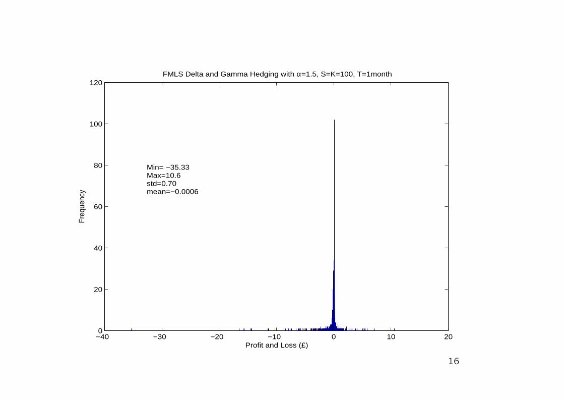
120FMLS Delta and Gamma Hedging with α=1.5, S=K=100, T=1month

Profit and Loss (£)

Freq

uenc

y

Min= −35.33Max=10.6std=0.70mean=−0.0006

16

FMLS Black-Scholes: the Taylor expansion view

dV (x, t) =∂V (x, t)

∂tdt +

∂V (x, t)

∂xdx

+1

Γ(2− α)Dα

+V (x, t)(dx)α + · · · .

(Samko et al 1993).

Therefore it seems natural, in the FMLS case, to delta and

fractional-gamma hedge the portfolio P (x, t) = V1(x, t) −∆ex −bV2(x, t), hence

a =∂V1(x, t)

∂x

1

ex− ∂V2(x, t)

∂x

1

exb

and

b =exDα

+V1(x, t)− ∂V1(x, t)/∂xDα+ex

exDα+V2(x, t)− ∂V2(x, t)/∂xDα

+ex.

17

−2 0 2 4 6 8 100

20

40

60

80

100

120

Profit and Loss (£)

FMLS Delta and Fractional Hedging with α=1.5, S=K=100, T=1monthFr

eque

ncy

Min= −1.2Max=8.4std=0.17mean=0.001

18

In General might want to do...

rV (x, t) =∂V (x, t)

∂t+ µ

∂V (x, t)

∂x+ GV (x, t), (3)

where G is an operator containing the fractional derivatives.

P (x, t) = V1(s, t;T1)− aex − bV2(s, t;T2) (4)

Therefore we require

a =∂V1(x, t)

∂x

1

ex− ∂V2(x, t)

∂x

1

exb

and

b =exGV1(x, t)− ∂V1(x, t)/∂xGex

exGV2(x, t)− ∂V2(x, t)/∂xGex

so the portfolio is both Delta and Fractional-Gamma-neutral, ie

∂P (x, t)

∂x= 0 and GP (x, t) = 0.

19

−60 −40 −20 0 20 400

5

10

15

20

Pofit and Loss (£)

Freq

uenc

yLS Delta Hedging, α=1.7, S=K=100, T=1month

Min=−408Max=5.2764Mean=−0.055

20

−8 −6 −4 −2 0 2 4 6 80

10

20

30

40

50

60

70

Profit and Loss (£)

Freq

uenc

yLS Delta and Gamma Hedging, α=1.7, S=K=100, T=1month

Min=−56Max=2.89Mean=0.0024

21

−1.5 −1 −0.5 0 0.5 1 1.50

10

20

30

40

50

60

Profit and Loss

Freq

uenc

yLevy−Stable Delta and Fractional Hedging, α=1.7, S=K=100, T=1month

Min=−20.64Max=2.29Mean=−0.0001

22

CONCLUSIONS and FURTHER WORK

For Levy processes with Levy densities that have a polynomial

singularity at the origin and exponential decay at the tails we can

recast the pricing equation in terms of Fractional derivatives.

The non-local property of the fractional operators can be useful

when dynamically hedging options.

Using well established numerical schemes for Fractional opera-

tors it might be possible to price American options. Moreover,

for these processes we can derive Fractional Fokker-Planck equa-

tions that may also be used in the pricing of American options.

23