the bell system technical journal - world radio history
TRANSCRIPT

THE BELL SYSTEM
TECHNICAL JOURNALDEVOTED TO THE SCIENTIFIC AND ENGINEERING
ASPECTS OF ELECTRICAL COMMUNICATION
Volume 54 July-August 1975 Number 6
Copyright Q 1975, American Telephone and Telegraph Company. Printed in U.S.A.
A Molded -Plastic Technique for Connectingand Splicing Optical -Fiber Tapes
and Cables
By P. W. SMITH, D. L. BISBEE, D. GLOGE, and E. L. CHINNOCK(Manuscript received September 25, 1974)
We describe a new technique for optical -fiber cable connecting andsplicing. Preliminary tests with multimode fibers produced splices with anaverage loss of less than 0.1 dB and a peak loss of 0.18 dB.
I. INTRODUCTION
Despite the efforts of many investigators,' -'2 the problem of con-necting and splicing optical -fiber cables and subgroups of fibers"(tapes) has remained a serious one. The continued improvement ofoptical fibers to the point where losses approaching 1 dB/km have nowbeen achieved" has made it increasingly apparent that practical con-nectors and splices should have losses much lower than those initiallyconsidered.
Someda4 demonstrated a splicing technique in which individualfibers are aligned by pressing them into a grooved substrate. Muchsubsequent work has involved extensions and improvements of thisidea. Miller' used precision -grooved aluminum spacers and preparedthe fiber ends by grinding and polishing. Cherin" used embossedgrooves and devised a jig for inserting tapes with previously preparedfiber ends into these grooves. The lowest losses in splices based on thistechnique were obtained by Chinnock et al.," who prepared the endsof the fibers using a fiber -fracture technique.' All these methods, how-ever, have drawbacks resulting either from difficulties associated
971

with the preparation of the fiber ends or with the mechanical align-ment of the previously prepared ends. These problems may makesuch techniques difficult to apply in the field.
In this paper we describe a new fiber -splicing technique that elimi-nates some of the difficulties associated with the grooved substratetype of splices, can function as a removable connector, and should bereadily adaptable for field use.
II. THE MOLDED -PLASTIC SPLICING TECHNIQUE
The basic technique is illustrated in Fig. 1. The end of the tape tobe spliced is prepared for molding by dissolving the plastic coatingover a short region (,:.-is 1 cm) to expose the individual fibers. The tapewith the exposed fibers is then placed in the mold as shown in Fig. la.The fibers are held accurately in position by means of a thin spacerplate (see insert). After a suitable plastic material is molded aroundthe fibers, the entire assembly is removed from the mold (Fig. lb).The fibers are exposed over a narrow region where the spacer plateheld them in position in the mold. The exposed fibers are now scored,and the entire assembly is fractured by bending and applying ten-sion in the manner previously described for single fibers.' The plasticmaterial fractures in the same plane as the optical fibers, and thetape termination is now ready for splicing (Fig. 1c). To make asplice, two tapes with terminations prepared as described above areplaced in an alignment channel, and a suitable index -matching epoxyis used to index -match and to hold the assembly together (Fig. 1d).
The splicing technique described above has a number of importantfeatures. Each operation is relatively simple and involves no handlingof individual fibers. The fiber -breaking technique quickly producesclean ends of good optical quality. Minimal handling of the preparedends is required. The technique can easily be adapted to make a re-movable connection.
To demonstrate these ideas, a mold was constructed as shown inFig. 2. The mold was machined from brass and was made in twoparts so that it could be taken apart to facilitate the removal of themolded tape ends. The spacer plate was made from 175 -Am steel feelergauge stock which was tapered to about 100 Am at the top. Figure 2bshows a close-up of the spacer plate.
Because polyester resin* is readily available, has a low initial vis-cosity, and shrinks little on hardening, it was used as the molding
* The polyester resin used for these experiments was No. 50111, Berton Plastics,Inc., South Hackensack, N. J.
972 THE BELL SYSTEM TECHNICAL JOURNAL, JULY-AUGUST 1975

(a) MOLD WITH PREPAREDFIBER RIBBONIN PLACE
(b) ENCAPSULATED RIBBONREMOVED FROM MOLDAND INVERTED
(C) PREPARED END
INDEX -MATCHINGEPDXY
(d) COMPLETED SPLICE
FIBER RIBBON -
Fig. 1-The molded -plastic fiber -tape splicing technique.
CONNECTING OPTICAL FIBERS 973

I I I
0 1 2 3
CENTIMETERS
(a)
SPACERPLATE
(b)
Fig. 2-Photograph of the mold used for these experiments. (a) Overall view. (b)Close-up view of precision spacer.
material, even though it required curing for several hours at ap-proximately 50°C. Low -shrinkage plastics are available, however, thatcure in a short time at room temperature.*
The optical -fiber tapes used for these splicing experiments weremade from multimode silicate glass fibers of 120 -Am outer diameter and80 -Am core diameter. The numerical aperture of these fibers wasmeasured to be 0.15. The fibers were made into tapes by dipping 2-mlengths of fiber into a solution of plastic materia115t and then slowly
* For example, Facsimile, made by Flexbar Machine Corp., Farmingdale, NewYork.
t The coating material used was 3M Kel-F-800, a co -polymer of vinylidene fluorideand chlortrifluoroethylene.
974 THE BELL SYSTEM TECHNICAL JOURNAL, JULY-AUGUST 1975

withdrawing the fibers. In this way, a 25 -/Am plastic coating was ap-plied to the fiber. To eliminate crosstalk between fibers, a black dyewas mixed with the coating material. The plastic -coated fibers werethen fused into a linear array using the technique previously developedby Eichenbaum.15
Figure 3 shows a section of five -fiber tape with the plastic materialremoved in preparation for splicing. The material was easily removedby applying acetone with a cotton swab. The next step in the splicingoperation involves placing the prepared tape in the mold shown inFig. 2. To hold the fibers positively in the grooves of the spacer plate,a slight tension was applied to the tape by clamping it to the springsteel extensions on either side of the mold (see Fig. 2). Because themold we were using was somewhat wider than the tape, we also placedpads on either side of the tape to hold the fibers straight as they passedover the spacer plate. Such pads would not be required if a narrowermold were used. Small pads of balsa wood were also used on top of thetape about 1 cm on either side of the spacer to ensure that the fibersremained pressed into the spacer grooves during the molding process.Polyester resin was then poured around the fibers, the lid of the mold
Fig. 3-Fiber tape with plastic material removed in preparation for placing in mold.
CONNECTING OPTICAL FIBERS 975
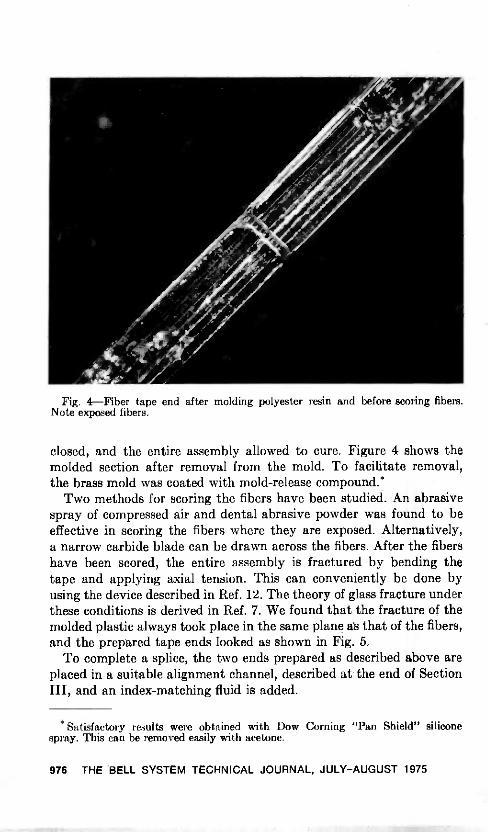
Fig. 4-Fiber tape end after molding polyester resin and before scoring fibers.Note exposed fibers.
closed, and the entire assembly allowed to cure. Figure 4 shows themolded section after removal from the mold. To facilitate removal,the brass mold was coated with mold -release compound.*
Two methods for scoring the fibers have been studied. An abrasivespray of compressed air and dental abrasive powder was found to beeffective in scoring the fibers where they are exposed. Alternatively,a narrow carbide blade can be drawn across the fibers. After the fibershave been scored, the entire assembly is fractured by bending thetape and applying axial tension. This can conveniently be done byusing the device described in Ref. 12. The theory of glass fracture underthese conditions is derived in Ref. 7. We found that the fracture of themolded plastic always took place in the same plane as that of the fibers,and the prepared tape ends looked as shown in Fig. 5.
To complete a splice, the two ends prepared as described above areplaced in a suitable alignment channel, described at the end of SectionIII, and an index -matching fluid is added.
* Satisfactory results were obtained with Dow Corning "Pan Shield" siliconespray. This can be removed easily with acetone.
976 THE BELL SYSTEM TECHNICAL JOURNAL, JULY-AUGUST 1975

Fig. 5-Tape end after scoring and fracturing. Note the polyester resin breaks inthe same plane as the optical fibers.
III. SPLICE LOSS MEASUREMENTS
The accurate measurement of small losses in good fiber -tape splicesrequires each fiber of the tape to be excited in the same way and withthe same amount of light. Repeatable and stable focusing of the inputbeam on a given spot within the fiber core is a prerequisite. To ac-complish this, we built the launching assembly shown in Fig. 6,
which is rigidly attached to a commercially available HeNe laser.The assembly not only holds the fiber tape and shields it and the laserbeam from dust and air movement, but also permits a precise visualalignment by way of a built-in microscope. The tape is epoxied to atape holder which slides into a micropositioner from the right of Fig. 6.A three-way alignment of each fiber -front face with the focus of thelaunching lens is possible (only one positioning screw is shown).
The launching lens, the beam splitter, and the eyepiece form amicroscope arrangement that provides a magnified view of the frontend of the tape. When the beam is launched into one of the fiber cores,the entire core area lights up as a result of back -scattered light fromthe inside of the fiber. A cross hair built into the eyepiece facilitatesthe alignment of beam focus and fiber core. The beam splitter alsoserves as an attenuator and deflects a portion of the laser beam ontoa silicon detector that provides a reference signal proportional to theinput light power. As the circuit diagram of Fig. 7 indicates, both thetransmitted signal and the reference signal are compared in a ratiometer where the result is displayed in digital form. This measuringtechnique, together with the precise visual alignment, was found toreproduce the excitation of each fiber to within ±0.01 dB over aperiod of at least one hour.
CONNECTING OPTICAL FIBERS 977

coOD
HeN
e LA
SE
R
1 f
--5X
EY
EP
IEC
E
-- M
ICR
OS
CO
PE
RE
TIC
LE
EX
PA
ND
ING
LE
NS
AS
SE
MB
LY
II
\I
I
/Q
UA
RT
Z/ /
10-d
BA
TT
EN
UA
TO
R/
FLA
T-B
EA
MS
ILIC
ON
AN
D B
EA
MLE
NS
DE
FLE
CT
OR
DE
TE
CT
OR
SP
LIT
TE
RF
= 6
.1m
m
FIB
ER
TA
PE
ir
II
Fig.
6-A
ppar
atus
use
d fo
r lo
ss m
easu
rem
ents
.
SP
RIN
G-M
OU
NT
ED
FIB
ER
-TA
PE
HO
LDE
R

LAUNCHINGASSEMBLY
HeNe LASER
REFERENCESIGNAL
FIBERTAPE
FIBERTAPE
DETECTORSPLICE
DETECTOR
POWERMETER
DIGITALRATIO
METER
OUTPUTSIGNAL
POWERMETER
Fig. 7-Cross section of beam -launching assembly.
Radiation losses of the above order of magnitude (0.01 dB/m) canbe incurred in the high -order modes as a result of minute bends alongthe fiber. The bends, and hence the loss, depend on the particularplacement of the fiber and its holding fixtures, and can change duringthe breaking and splicing operation. To minimize the influence of thiseffect, the focal length of the launching lens is chosen to excite anumerical aperture of 0.10 out of the total numerical aperture of 0.15,so that some of the high -order modes are not excited. On the other hand,these modes may participate to some extent in the transmission (andin the splice loss), if long fiber lengths are involved. The resultingchange in splice loss is expected to be small, but needs to be explored.
Our splicing tests were conducted by making two molded sectionsapproximately 10 cm apart near the center of a 2-m length of tape.The same mold in the same orientation was used for each moldedsection. Prior to the splicing test, the transmission of each fiber in theunbroken tape was measured using the apparatus previously described.The two molded sections were then fractured, the center 10 -cmsection removed, and the two ends replaced in the mold. A drop ofglycerine was added for index -matching, and the ends of both moldedsections were held down with a single Teflon* blade about 1 mm inwidth. The transmission of each fiber was again measured.
Figure 8 is a histogram of the measured losses for tests on 20 fibers,and Fig. 9 shows the cumulative loss distribution. In two cases, eitherbecause of inadequate scoring or because of a weak region in thefiber, a fiber fractured at a point other than the desired fracture point.These cases have not been included in our data. Also omitted are three
" Registered trademark of Dupont Corporation.
CONNECTING OPTICAL FIBERS 979

0 0.05 0.10 0.15
LOSS IN DECIBELS0.20
Fig. 8-Histogram of loss measurement data.
cases where fibers in one of the tapes were broken during handling.The average measuring error for these experiments was found to be0.01 dB. No correction for this scatter was applied to the data.
Permanent splices were made using epoxy instead of glycerine as anindex -matching material. This not increase the splice loss
100
90
80
70
60
50
40
30
20
10 - //./. I
0
1 I
0-41
0.05 0.10 0.15 0.20 0.25
SPLICE LOSS IN DECIBELS
Fig. 9-Cumulative distribution of measured splice losses.
980 THE BELL SYSTEM TECHNICAL JOURNAL, JULY-AUGUST 1975

Fig. 10-Completed splice using brass alignment channel and epoxy cement bothfor index matching and for holding the assembly together.
mold was used as an alignment channel. To make more compact andpermanent splices, we epoxied molded tape ends into either a channelmade from 125 -pm -thick phosphor bronze sheet or a 1 -mm -by -0.3 -mmmilled brass channel, as shown in Fig. 10. The resulting loss increaseof between 0.1 and 0.3 dB was attributed to imperfections of the moldthat were reproduced in the molded ends. The use of alignment sleevesto alleviate this problem is discussed in the next section.
IV. DISCUSSION AND CONCLUSIONS
The splice losses reported in Section III are lower than those re-ported for other splice techniques9,'° and are comparable with the losseswe have observed using a grooved substrate to align fibers withpreviously prepared ends.'2 We believe, however, that the techniquedescribed in this paper has a potential for adaptation to a variety offiber -connector problems and to field splicing of fiber cables.
There are two "precision" operations involved in our splicingtechnique, (i) the intial placing of the prepared fiber tape in the moldand (ii) the placing of the molded ends in the holder. Suitably designedmolding tools and alignment sleeves should facilitate these operationsto the point where they require no special skills. One importantproblem is that of maintaining a high degree of cleanliness. If thesame mold is used to prepare both ends to be spliced and this mold
CONNECTING OPTICAL FIBERS 981

is also used as the alignment channel, a high -precision mold is notrequired. If, on the other hand, the prepared ends are to be joined in adifferent alignment channel, precision molds must then be used. Theuse of precision molds does not present a major problem, however, forthe molds can be made, tested, and cleaned in advance, and thesemolds can, at a later time, be prepared for reuse. In this case, separatemolds would be used to prepare each tape end; we thus avoid theproblems inherent in the first -described technique associated withcleaning a mold in the field.
A definitive design of the alignment channel is beyond the scopeof this work, since this design must depend considerably on theconstraints of a specific connection : a removable or permanent con-nection of one fiber tape inside a building, for example, has differentrequirements from a cable field splice. However, some guidelinescommon to all designs can be extracted from our work : the referencesurfaces used for the alignment of two molded terminations should benarrow and well defined to avoid misalignment as a result of moldirregularities and contamination. Thus, rather than using the channelof Fig. 10, which encloses the terminations on three sides, a sleeve thatmakes contact with the terminations only along their narrow sidesmay be more practical. More specifically, the sleeve might comprisetwo V -grooves designed to accept the V-shaped narrow sides of ter-minations molded in the shape shown in Fig. 11. The width of theV -grooves should be somewhat wider than the thickness of the ter-minations so that contact is only made along the grooves and not atthe top and bottom surface of the molded piece. Besides minimizingand defining the alignment surfaces, this approach permits a space -saving and simple arrangement of stacks of terminations in the caseof a fiber cable, as illustrated in Fig. 11. This figure shows two groovedchips spring -mounted opposite each other inside a cartridge that alignsthe terminations and serves as the inside housing and protection forthe cable splice.
This approach, together with the molding technique, seems partic-ularly well suited to produce removable connections. In this case, theindex -matching epoxy or liquid would be advantageously replaced bya gel that can easily be removed when the connection is dismantled.When such terminations are prefabricated in the factory, the tech-nique proposed here offers the additional advantage that the termina-tions can be delivered unfractured, so that the end faces remain pro-tected until they are fractured on site shortly before the connection ismade.
In conclusion, we have described and demonstrated a new splicingtechnique for optical fiber tapes that yields an average splice loss of
982 THE BELL SYSTEM TECHNICAL JOURNAL, JULY -AUGUST 1975

SLE
EV
E
MO
LDE
D T
ER
MIN
AT
ION
S
- F
IBE
R C
AB
LE
MO
LDE
D T
ER
MIN
AT
ION
S--
....
GR
OO
VE
D A
LIG
NM
EN
T C
HIP
Fig.
11-
Gro
oved
alig
nmen
t sle
eve
for
cabl
e sp
licin
g an
d co
nnec
tors
.

less than 0.1 dB. This technique involves no handling of individualfibers and alleviates some of the difficulties of fiber -end preparation andmechanical alignment of previously prepared ends that are encounteredwith other techniques.
An adaptation of our technique for field use would involve develop-ing a molding technique applicable at room temperature with a quick -setting plastic encapsulating material and the design of molding toolsand alignment sleeves to facilitate the joining operation.
REFERENCES
1. D. L. Bisbee, "Optical Fiber Joining Technique," B.S.T.J. 50, No. 10 (December1971), pp. 3153-3158.
2. R. B. Dyott, J. R. Stern, and J. H. Stewart, "Fusion Junctions for Glass FiberWaveguides," Elec. Letters, 8, (June 1973), pp. 290-292.
3. 0. Krumpholz, "Detachable Connector for Monomode Glass Fiber Wave -guides," Archiv Elektronik Vbertragungstechnik, 26 (1972), pp. 288-289.
4. C. G. Someda, "Simple Low -Loss Joints Between Single -Mode Optical Fibers,"B.S.T.J., 52, No. 4 (April 1973), pp. 583-596.
5. A. H. Cherin, E. R. Eichenbaum, and M. I. Schwartz, "Splicing Optical FiberRibbons, First Attempts," unpublished work.
6. A. H. Cherin, "Multi -Groove Embossed Plastic Splice Connector for OpticalFibers, A Feasibility Study," unpublished work.
7. D. Gloge, P. W. Smith, D. L. Bisbee, and E. L. Chinnock, "Optical Fiber EndPreparation for Low -Loss Splices," B.S.T.J., 52, No. 9 (November 1973), pp.1579-1589.
8. H. W. Astle, "Optical Fiber Connector with Inherent Alignment Feature,"unpublished work.
9. C. M. Miller, "A Fiber Optic Cable Connector," B.S.T.J., November 1975.10. A. H. Cherin and P. J. Rich, "A Splice Connector for Joining Linear Arrays of
Optical Fibers," in Optical Fiber ?transmission (digest of technical paperspresented at the topical meeting on optical fiber transmission, January 7-9,1975, Williamsburg, Va.), Optical Society of America, pp. WB3-1 to WB3-4.
11. R. M. Derosier and J. Stone, "Low -Loss Splices in Optical Fibers," B.S.T.J., 52,No. 7 (September 1973), pp. 1229-1235.
12. E. L. Chinnock, D. Gloge, P. W. Smith, and D. L. Bisbee, "Preparation ofOptical Fiber End for Low -Loss Tape Splices," B.S.T.J., 54, No. 3 (March1975), pp. 471-477.
13. R. D. Standley, "Fiber Ribbon Optical Transmission Lines," B.S.T.J., 53, No. 6(July -August 1974), pp. 1183-1185.
14. W. G. French, J. B. MacChesney, P. B. O'Connor, and G. W. Tasker, "OpticalWaveguides with Very Low Losses," B.S.T.J., 53, No. 3 (May -June 1974),pp. 951-954.
13. B. Eichenbaum, "A Technique for Assembling Fiber Optic Arrays," unpublishedwork.
984 THE BELL SYSTEM TECHNICAL JOURNAL, JULY -AUGUST 1975

Copyright © 1975 American Telephone and Telegraph CompanyTHE BELL SYSTEM TECHNICAL JOURNAL
Vol. 54, No. 6, July -August 1975Printed in U.S.A.
Coupled -Mode Theory for AnisotropicOptical Waveguides
By D. MARCUSE(Manuscript received December 11, 1974)
The well-known coupled -mode theory of waveguides is extended to in-clude dielectric guides made of anisotropic materials. Exact coupled -waveequations for anisotropic dielectric waveguides are derived, and explicitexpressions for the coupling coefficients are given. The coupling coefficientsfor isotropic waveguides are obtained as a special case. A simple approxi-mation for the coupling coefficients in the case of slight anisotropy andslight departure from an ideal waveguide is presented.
I. INTRODUCTION
The theory of dielectric optical waveguides deals with electro-magnetic wave propagation in optical fibers and in the waveguidesused for integrated optics. Wave propagation in these structures isdescribed in terms of normal modes.'-' However, normal modes pre-serve their identity only in perfect waveguides without irregularitiesof either the refractive index distributions or the waveguide geometry.Electromagnetic wave propagation in waveguides with any kind ofirregularities must be described by means of coupled -mode theory.3.4The electromagnetic waves in imperfect waveguides are expressed assuperpositions of all the modes of a perfect waveguide. The modeamplitudes are coupled together by coupling parameters that dependon the nature of the waveguide imperfections. A description of wavepropagation by means of coupled -mode theory allows calculation ofradiation losses caused by intentional or unintentional fluctuations ofthe refractive index along the axis of the waveguide or by core -claddingboundary fluctuations." Coupling among guided modes is used todesign modulators or distributed feedback circuits for lasers or toeffect improvements in the multimode dispersion properties of over-moded waveguides. The coupled -mode theory is well developed forwaveguides that consist of isotropic dielectric materials.33 Some workhas been done to extend this theory to waveguides consisting of aniso-tropic materials.5-7 These waveguides are assuming increasing im-
985
portance in integrated optics as methods are being perfected forfabricating waveguides by diffusing different dopants (or outdiffusionof certain component atoms) into anisotropic crystals.8-w
This paper describes the derivation of coupled -wave equations forthe modes of waveguides consisting of anisotropic materials. Thecoupled -wave theory is based on the definition of guided and radiationmodes as solutions of Maxwell's equations for idealized structures. Anorthogonality relation is derived that is needed to isolate individualterms in the infinite series expansion of the electromagnetic field. Theprincipal result of this theory is the derivation of coupling coefficientsthat are important for solving coupled -mode problems. Readers notinterested in the derivation should look at eqs. (46) and (48). Applica-tions of this theory are not presented here, since they will be the sub-ject of further publications.
II. THE FIELD EQUATIONS FOR ANISOTROPIC MEDIA
The derivation of coupled -wave equations for anisotropic dielectricwaveguides follows closely the procedure used for deriving coupled -wave equations for isotropic waveguides.3 The objective of coupled -wave theory is to construct solutions of Maxwell's equations for wave -guiding structures consisting of general refractive -index distributions.
Anisotropic media are characterized by a dielectric tensor,
(exx exY eXZ
E = Eyx Eyy Eyz
ezx ezy eZZ
(1)
We assume that the elements of this tensor are real quantities char-acteristic of lossless materials. It can be shown that conservation ofenergy requires that the dielectric tensor form a symmetric matrixso that the following relations hold :11
ex?, = ey.: exz = ezz, fyz = ezy (2)
The magnetic properties of the medium are assumed to be the sameas that of a vacuum so that we use the (isotropic) magnetic permea-bility constant µo. Maxwell's equations for anisotropic media assumethe form
V X H = icoeE
V X E = - icoµ011.
(3)
(4)
It was assumed that the electric field vector E and the magnetic fieldvector H have the time dependence,
eicut.
986 THE BELL SYSTEM TECHNICAL JOURNAL, JULY -AUGUST 1975
(5)

The tensor notation EE may be expressed in component form as
(EE)i = EijEj. (6)
Summation over double indices is understood, and the subscripts iand j assume the values 1, 2, and 3 that represent the x, y, and zcomponents of the vector E or tensor E.
Derivation of coupled -wave equations for isotropic media is facil-itated by expressing the longitudinal components of E and H in termsof the transverse components.' This practice is preserved for our deriva-tion of coupled equations for anisotropic media. We single out the zcoordinate as the direction of the waveguide axis and express the fieldvectors and the differential operator V as superpositions of transverseand longitudinal parts. The symbol t indicates the transverse direc-tions x and y. Thus, we have
E = El Ez, (7)
= 11/ ± Hz, (8)
and
V = V/ az(9)
We use the notations ex, ey, and ez to indicate unit vectors in x, y,and z directions.
The transverse part of the vector E is indicated by the notationEt E or, in component notation,
exE = ez(e.X. + Exy.Ey ezzEz) (10)
evE = ey(EvzEx eyyEy Ev.Ez). (11)
The longitudinal part is
ezE = ez(ez.Ex ezuEy EzzEz) (12)
We may now separate Maxwell's equations into transverse and longi-tudinal parts. The transverse parts of (3) and (4) are
v, X H, ez X = icoet E (13)
V, X Ez8E ,
ez X = - iwµoHt. (14)
Their longitudinal parts may be written as
V/ X H, = ico(ezE/ EzzEz) (15)
andVi X E, = - itolhollz (16)
COUPLED -MODE THEORY 987

The longitudinal parts of E and H follow immediately from (15) and(16),
and
Ez = .
1 v, X Ht - -1 ezEticuezz fzz
Hz = - 1V't X Et.
twilo
(17)
(18)
On the right-hand side of (17) and (18) appear only transverse com-ponents of E and H. It is important to distinguish between the singleand double subscript notation of E. A double subscript, like ezz, indi-cates a single tensor element of e, while a single subscript, like ez, isdefined by (10) through (12). In particular, we have
Ez Et = ez(ezzEr ezyEy). (19)
We now use (17) and (18) to eliminate the z components of E and Hfrom the transverse parts of Maxwell's equations (13) and (14),
aH ,-zW120
v, X (v, x Et) -azez X
= iCOEt E t -iC0- et ezEt + -1 et (v, X HO (20)ezz ezz
and0E,
v, X - -1 EzEt] ez X -az = - (21)twEzz ezz
These two vector equations represent four scalar equations. Onceeqs. (20) and (21) are solved, the z components of E and H can beobtained by simple differentiation from (17) and (18). We have thusachieved a simplification of the original problem by reducing the num-ber of equations from six, in (3) and (4), to only four.
The components of the e tensor are assumed to be functions of x, y,and z. The E tensor defines the wave -guiding structure. Because of thez dependence of E, eqs. (20) and (21) do not have mode solutions. Anormal mode is defined as a solution of Maxwell's equations whose zdependence can be expressed by the simple function
(22)
Such solutions exist only if the dielectric tensor does not depend onthe z coordinate. To construct solutions of the general eqs. (20) and(21), we consider solutions of simpler equations that are defined bya tensor a that is similar to E but is independent of z. The choice ofis obviously arbitrary and is determined by convenience. Using (22),we find from (20) and (21) the following equations for the normal
988 THE BELL SYSTEM TECHNICAL JOURNAL, JULY -AUGUST 1975

modes of the waveguide structure defined by
1- v1 X (V1 X Cr) - i13!,P)ez X 30,11)icomo
= iwir - i-w + -1 it (V1 X 30/))ezz E.
and
Vi X [ .
1V/ X 3C,11) -
1E,E(//)]
1WEzz
(23)
- f,P)ez X CP = - icol.403Cfr. (24)
The subscript v indicates a mode label. Equations (23) and (24) admitan infinite number of solutions with different eigenvalues (propagationconstants) )3P) and different field vectors C,P) and 3C?). Script lettersindicate mode fields, while roman letters E and H are reserved for gen-eral field distributions. The modes are of two different types, guidedmodes whose fields are confined to the vicinity of the waveguide andradiation modes that extend to infinity in transverse direction to theguide.2.3 Guided modes have discrete eigenvalues IV), while the eigen-values of radiation modes form a continuum. The superscript (p)stands for either (+) or (- ), depending on the direction of wavepropagation. A wave traveling in the positive z direction has positive(real) values (3;,+), a wave traveling in the negative z direction has anegative (real) value 13Y"). In isotropic media, we have the simplerelations,
and
= - (25)
C.7) = g(pt), = - Ct.), (26)
Se!,7) = - 30,;) = (27)
General anisotropic media are more complicated, so that (26) to (27)do not apply. Modes traveling in one direction may be different frommodes traveling in the opposite direction.
III. ORTHOGONALITY RELATIONS
The modes of anisotropic dielectric waveguides are mutuallyorthogonal.2 For the purpose of deriving orthogonality relations, it issimpler to use Maxwell's equations in the form (3) and (4) instead ofthe form (23) and (24). Separating the z derivatives from the Voperator, we write (3) for a mode labeled v and (4) for a mode labeled A,
vt X 30,P) - 0;,P)ez X 30,P) = i(,) E(P) (28)
VI X 8:!) - 0:4°)e. X 8,(!) = - icopoRig). (29)
COUPLED -MODE THEORY 989
and
Next, we take the complex conjugate of (28), multiply the resultingequation by gr, multiply (29) by -3ef,P)*, add the two equations, andintegrate over the infinite cross section (i is assumed real) :
J JX 3C (pp)* - 3c!,P)* x
ii3;,P)*&:!)ez X 3C ,1))* i3r3C;,P)*ez X g:,q)}dxdy
= - iwf f [&!) i C,P)* - 03C ;,P)* ae,q)]c/xdy. (30)
The first two terms on the left-hand side of (30) can be expressed as
-f rot. W,q) X 3C;,P)*)dxdy = -f (&,q) X 3cf,P)*).nds. (31)
The two-dimensional divergence theorem was used to convert theintegral over the infinite cross section in the x -y plane to an integralover the infinite circle with outward normal direction n and line ele-ment ds. The integral on the right-hand side vanishes if at least oneof the two modes is a guided mode. If both modes v and µ are radia-tion modes, the integral vanishes in the sense of a delta function ofnonzero argument.2 Using this fact and a well-known vector identity,we can express (30) as
(13 ,(hg) - #;P)*) f (iµ4)ez,q) X 3.CP)*)dxdy
= - f [8Q) E &I,P)* - 143C,,Q) 3C(P)*]dxdy. (32)
Because of the symmetry of the E tensor, the following relation holds:8(p)*. g g(4) = g,(!) . C,P)* (33)
We take the complex conjugate of (32), interchange the superscripts pand q as well as the subscripts v and g and, using (33), subtract thenew expression from (32) with the result :
(3,(!) - 3(P)*) f fez [8,(!) X 3C?)* gf,")* X 3C,(!)]dxdy = 0. (34)
Equation (34) is the desired orthogonality relation. It is obvious thatthis expression holds also for isotropic media. However, in the iso-tropic case it is possible to use (25) through (27) to prove that eachterm in (34) must vanish separately.2 For the general anisotropic case,(34) cannot be simplified further. We infer from (34) that the integralvanishes if or - tv)* 0. This means that the integral vanishes evenin the case v /I if p and q indicate opposite signs, and a wave isorthogonal to its backward traveling counterpart (if )3f,g) is real) if
orthogonality means vanishing of the integral in (34).
990 THE BELL SYSTEM TECHNICAL JOURNAL, JULY -AUGUST 1975
The integral in (34) expresses the total power flow if v = AL andp = q. We may therefore use the orthonormality relation,
fez NV X 3C V' &,(,f)* X 3er]dxdy
= 2s(g)#" *"q)(14e l PS, (35)
to express mode orthogonality and normalization. The subscripts tindicating the transverse parts of the modes were added since the zcomponents of the fields do not contribute to (35). P is a normalizingfactor common to all modes that is used to adjust the arbitrary ampli-tudes of the normal modes. For real values of (3f"), we have
= 1. (36)
In this case, the sign of the integral is expressed correctly by the factthat (3,g) reverses its sign if q goes from (+) to (-). For opposite signsof p and q, the right-hand side of (35) vanishes as required by (34)if 13f,°) is real. For imaginary 0;,°), (35) vanishes for q = p. The orthog-onality relation also holds for imaginary values of 13v°). Imaginaryvalues of the propagation constants occurs only for evanescent "radia-tion" modes.2.3 In the case of imaginary (), the sign of the right-handside of (35) is not certain. For this reason, we have introduced the factors,(,°) that must be adjusted so that P is a positive real quantity. Thismeans that .1) may have to be negative, s,(,e) = - 1. However, thiscase can arise only in connection with evanescent "radiation" modes.The S symbol in (35) indicates Kronecker's delta if both modes areguided. When one mode is guided while the other is a radiation mode,we have S = 0. If both modes are radiation modes, S must beinterpreted as the Dirac delta function.
IV. DERIVATION OF COUPLED -WAVE EQUATIONS
Any arbitrary field distribution compatible with Maxwell's equationscan be expressed as the superposition of all the modes of the idealizedstructure defined by the dielectric tensor E. Because the complete setof modes consists of a finite number of guided modes plus a continuumof radiation modes, we express the transverse parts of a general fieldby the expansion
Et = E a,Y)C71) E L'a(P) (p) giP) (p)dpv,p
and
Ht = E a;,P)X,(,f) E a (")(P)3W)(P)dP
(37)
(38)
COUPLED -MODE THEORY 991

The longitudinal parts follow from (17) and (18). The superscriptsassume the values (+) and ( -) indicating waves traveling in positiveand negative z direction. The first terms in (37) and (38) represent thecontribution of the finite number of guided modes labeled v. Thesecond terms indicated combinations of sums and integrals. Theintegration ranges over the entire region of continuous -mode labels pand includes radiation modes with real as well as imaginary values of,(3(P) (p). The summation symbol in front of the integral sign indicatesthat, in addition to modes traveling in positive and negative z direc-tion, various types of radiation modes exist and must be added toobtain the complete set of modes. For the purpose of deriving coupled -wave equations, the notation of (37) and (38) is too cumbersome. Weuse an abbreviated notation by omitting the integration sign, leavingit understood that the summation symbol includes summation overguided modes and summation as well as integration over radiationmodes. We thus write
E, = E a f,P) 8,T) (39)
and
I, p
H, = E f,P)3C,Y,'). (40)Y,P
gf,f) and 3C,7t)) are independent of z, but ct,P) is a function of z. Substitu-tion of (39) and (40) into (20) and (21) and use of the mode eqs.(23) and (24) leads to
P,p
E zo(P'clP))(ez X 3Cf,f))dz
da(P) .
= E a,(P) 110)(ft - it) E - ice (P,p ezz
anddace)
E tif3,P)a,P))(ez x Eft)p dz
et ez - 1 il iz) 8,91)ezz
( 1 1
ezzEt - EzzEt).
(171 X 30I)) (41)
E I X(
P,p iCO ezz gzz
( 1 1 iz). 00()pi
1}(42)
eZZ ZZ
We take the scalar product of (41) with - gg)* and of (42) with 3c,(ii)*,then we add the two equations, integrate over the infinite cross section,
992 THE BELL SYSTEM TECHNICAL JOURNAL, JULY-AUGUST 1975

and use the orthogonality relation (35). The result of this procedure is
9s(r)ca) #r* ( damP ± )?Or
Or I dz
= > a;,") f 1- ico eg)* (Et - it) &Tv,p
iw 60* ( eg.6. gtgz t- ) (Qt X 3C,11))Ez. gzz Ezz 6..
r1 ( 1
L to) \ ezz Zzz
Ez - ) C,11) dxdy. (43)ezz izz
On the left-hand side of (43), we have used a superscript (r) . Thisnotation is necessary to distinguish between the case of real and im-aginary propagation constants 0). If 0) is real, we have r = q. If0) is imaginary, as it is for evanescent radiation modes, we must choosefor r the sign opposite to q. We now write (43) in the abbreviated form
da(r) = - E KkV)a,(,P). (44)dz v,p
The coupling coefficient is defined by (43). We may eliminate thetransverse magnetic -mode field vector from the coupling coefficientby using (17) (applied to the mode field) and the identity (which is
obtained by partial integration),
ff 30)* (v, X F) dxdy = f f (V I X 3C(*) Fdxdy (45)
The coupling coefficient can be expressed as
cv) = I tr' f f {8 [ E. Et. Ez
4sro *pL ezz Ezz
- 0)**('" - o +
+ z 0)* z z &;(igz)*) [Ez-
- (et - t) J
1)(4! + C,V)ezz
Ez iz- -) s!)]}dxdy. (46)Ezz Zzz
V. IMPORTANT SPECIAL CASES
In its complete form, (46), the coupling coefficient is very compli-
cated. For isotropic media, where the E tensor degenerates to a multiple
COUPLED -MODE THEORY 993

of the unit tensor, (46) simplifies to the exact form,
Kv.P) = IQ r f(E -z)[gr* CP L" SO* 8,Vidxdy, (47)
4isr fir *P J Ezz
in complete agreement with the well-known result."In many practical applications, the anisotropy of the dielectric
medium is only slight, and the difference between the actual dielectrictensor E and the ideal tensor E is small. In that case, (46) can be sub-stantially simplified. A reasonable approximation of (46) for slightanisotropy and small values of E i is
KZ = '3r I f f g:ig)* (e - i) Ef,P)dxdy. (48)4isr
Note that the whole vectors of the electric mode fields enter (48) andnot just the transverse or longitudinal parts. The approximation (48)is obtained by considering off -diagonal elements and differences be-tween diagonal elements of E and E as quantities that are small of firstorder. Products of two first -order quantities have been neglected. Forreaders who did not follow the detailed derivation, we repeat herebriefly the definitions of symbols appearing in (46) through (48). Thesymbol co is the angular frequency of the electromagnetic field. Thescript symbols C,P) indicate the electric -field vectors of normal modesof an idealized waveguide that is defined by the dielectric tensorE = z(x, y), the subscript I, is a mode label, and the superscript (p)stands for either (+) or ( -), indicating the direction of wave propaga-tion. The propagation constants ,(sr) of the modes are labeled in thesame way as the field vectors. The superscript r is usually identicalwith the superscript q. Only in the case of imaginary Or (this casehappens for coupling to a nonpropagating radiation mode and is oflittle practical interest) does r indicate the sign opposite to q. Likewise,4r) = 1 for most cases of interest. Only for imaginary values of or mayit become necessary to choose 40 = -1 to keep the power normaliza-tion coefficient P positive in (35). The asterisk indicates complex con-jugation. Subscripts t and z occurring in (46) and (47) refer to thetransverse and longitudinal parts of the vectors to which they areattached. Similar subscripts attached to E are defined by (10) through(12) and (19). The dielectric tensor E = E(x, y, z) defines the actualwaveguide (in contrast to the ideal guide that is only a mathematicalfiction). The integrals are extended over the infinite transverse crosssection of the guide. Equation (48) assumes the same limit as (47) ifthe dielectric tensor degenerates into a multiple of the unit tensorsince, in the spirit of the approximation (48), we must use -zz, ezz = 1.
Equation (48), even though it is only an approximation, is likely to be
994 THE BELL SYSTEM TECHNICAL JOURNAL, JULY -AUGUST 1975

of most importance in practical applications because of its simple form.For many practical problems, the approximation is justified and leadsto sufficiently accurate results.
VI. CONCLUSIONS
We have derived coupled -wave equations representing exact solu-tions of the electromagnetic field problem for dielectric waveguidesthat consist of anisotropic materials whose dielectric tensor is a functionof the z coordinate. The field of the general waveguide is expressed interms of ideal modes of a hypothetical dielectric waveguide defined bya dielectric tensor whose elements are independent of the z coordinate.The main result of this paper is the expression (46) for the couplingcoefficients. For many practical applications, the exact coupling coeffi-cient- can be approximated in the simple form (48).
The coupled -mode theory for anisotropic dielectric waveguides isessential for the solution of problems of mode propagation in integrated -optics guides with random or systematic irregularities. A particularlyimportant area of applications are guides that are made anisotropicby an externally applied dc voltage or whose anisotropy is changed bysuch a voltage. Instead of an applied voltage, an acoustical wave maycause an anisotropic change of the refractive index of a dielectric wave -guide. These cases cannot be handled by the simpler isotropic coupled -mode theory, but require the extension to anisotropic media presentedhere.
REFERENCES
1. N. S. Kapany and J. J. Burke, Optical Waveguides, New York : Academic Press,1972.
2. D. Marcuse, Light Transmission Optics, New York: Van Nostrand Reinhold,1972.
3. D. Marcuse, Theory of Dielectric Optical Waveguides, New York: Academic Press,1974.
4. A. W. Snyder, "Coupled Mode Theory for Optical Fibers," J. Opt. Soc. Am., 62,No. 11 (November 1972), pp. 1267-1277.
5. S. Wang, M. L. Shah, and J. D. Crow, "Wave Propagation in Thin -Film OpticalWaveguides Using Gyrotopic and Anisotropic Materials as Substrates," IEEEJ. Quant. Elec., QE -8, Part 2, No. 2 (February 1972), pp. 212-216.
6. A. Yariv, "Coupled Mode Theory for Guided Waves," IEEE J. Quant. Elec.,QE -9, No. 9 (September 1973), pp. 919-933.
7. T. P. Sosnowski and G. D. Boyd, "The Efficiency of Thin -Film Optical -Wave -guide Modulators Using Electrooptic Films or Substrates," IEEE J. Quant.Elec., QE -10, No. 3 (March 1974), pp. 306-311.
8. I. P. Kaminow and J. R. Carruthers, "Optical Waveguiding Layers in LiNbO,and LiTa03," Appl. Phys. Letters, 22, No. 7 (April 1973), pp. 326-328.
9. J. M. Hammer and W. Phillips, "Low Loss Single -Mode Optical Waveguidesand Efficient High -Speed Modulators of LiNb.Tal_.03 and LiTa03," Appl.Phys. Letters, 24, No. 11 (June 15, 1974), pp. 545-547.
10. R. V. Schmidt and I. P. Kaminow, "Metal -Diffused Optical Waveguides inLiNbO,," Appl. Phys. Letters, 25, No. 8 (October 15, 1974), pp. 458-460.
11. M. Born and E. Wolf, Principles of Optics, 3rd Edition, New York : PergamonPress, 1964.
12. Ref. 3, p. 104, Eq. (3.2-44).
COUPLED -MODE THEORY 995

=i7gag..1011MINIMISOMB-

Copyright © 1975 American Telephone and Telegraph CompanyTHE BELL SYSTEM TECHNICAL JOURNAL
Vol. 54, No. 6, July-August 1975Printed in U.S.A.
Influences of Glass -to -Metal Sealing on theStructure and Magnetic Properties of an
Fe/Co/V Alloy
By M. R. PINNEL and J. E. BENNETT(Manuscript received December 26, 1974)
Apparent changes in the coercivity and remanence of the magnetic reedmaterial used in the remreed sealed contact were encountered during theglass -to -metal sealing operation. By using primarily metallographic ob-servations correlated with magnetic data, it was determined that thesechanges were due to a modification of the 600°C -aged microstructure causedby the time/temperature cycle experienced in sealing. The room -tem-perature stable precipitates that are developed by the 600°C anneal toproduce magnetic hardening are dissolved, and the alloy converts to a two-phase duplex body -centered cubic (Bcc) microstructure along one-half totwo-thirds of the reed shank. This produces a substantial increase in co-ercive force and some decrease in remanence. The structure and propertiesof the alloy before sealing have little influence on the reaction.
I. INTRODUCTION
A recent effort in the telecommunications industry has been thedevelopment of a remanent reed, sealed contact (remreed).' Oneproblem encountered in this development was an apparent change inthe magnetic properties of the Remendur (Fe, Co, V alloy) reed duringthe glass -to -metal sealing operation. During sealing, the reed can reachpeak temperatures in excess of 1050 °C and may be at temperatures inexcess of 900°C for as long as 8 to 10 seconds. Preliminary data suppliedto the authors indicated an increase in the coercivity of reeds from thesealing operation,' whereas the results of Kitazawa, Oguma, and Harashowed a 22 -percent decrease in coercivity at switch sealing.3 There-fore, a description of the exact nature of this change and an explana-tion of the mechanism by which it occurs were sought. Also, informa-tion on the possible influence of variations in the time/temperaturesealing cycle on the magnitude of this change was considered relevantto determine if improvements could be achieved by such modifications.
997
This paper summarizes the results of both a laboratory study on theRemendur alloy and evaluation of manufactured contacts to ascertainthe mechanism for the reported property changes. The normal sealingoperation was also modified by increasing the sealing speed and reduc-ing the sealing -lamp temperature to obtain data on possible modifica-tions to minimize the changes. Also presented are data on the influenceof microstructure from the prior strand -anneal and 600°C -aginganneal -heat treatments on the stability of the aged magnetic properties.
II. EXPERIMENTAL PROCEDURES
The evaluation on actual sealed reeds was carried out on WesternElectric Company assembled contacts. A group of reeds stamped froma single coil of commercially melted and processed 0.535 -mm Remendurwire was aged at 610°C in hydrogen for two hours. Some reeds of thisgroup were assembled into contacts at two separate manufacturingfacilities. Samples of the aged reeds and reeds that had been removedfrom these assembled contacts were supplied to the authors for evalua-tion (Experiment A). Additionally, contacts that had been sealed at anaccelerated speed were provided (Experiment B). Finally, a two -groupsample was supplied consisting of six typical contacts and six contactssealed with a 100-W reduction in power on the sealing lamps (Experi-ment C).
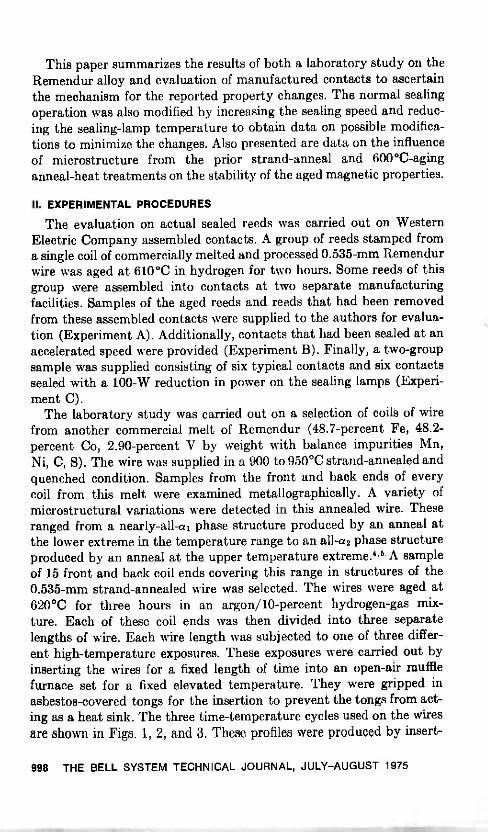
The laboratory study was carried out on a selection of coils of wirefrom another commercial melt of Remendur (48.7 -percent Fe, 48.2 -percent Co, 2.90 -percent V by weight with balance impurities Mn,Ni, C, S). The wire was supplied in a 900 to 950°C strand -annealed andquenched condition. Samples from the front and back ends of everycoil from this melt were examined metallographically. A variety ofmicrostructural variations were detected in this annealed wire. Theseranged from a nearly -all -al phase structure produced by an anneal atthe lower extreme in the temperature range to an all -a2 phase structureproduced by an anneal at the upper temperature extreme.4'5 A sampleof 15 front and back coil ends covering this range in structures of the0.535 -mm strand -annealed wire was selected. The wires were aged at620°C for three hours in an argon/10-percent hydrogen -gas mix-ture. Each of these coil ends was then divided into three separatelengths of wire. Each wire length was subjected to one of three differ-ent high -temperature exposures. These exposures were carried out byinserting the wires for a fixed length of time into an open-air mufflefurnace set for a fixed elevated temperature. They were gripped inasbestos -covered tongs for the insertion to prevent the tongs from act-ing as a heat sink. The three time -temperature cycles used on the wiresare shown in Figs. 1, 2, and 3. These profiles were produced by insert -
998 THE BELL SYSTEM TECHNICAL JOURNAL, JULY -AUGUST 1975
TYPICAL - SEALINGCYCLE (1)
1050 °C
-- 1000 °C
-- 800 °C
60 54 48 42 36 30 24 18 12 6 0
SECONDS
Fig. 1-Time/temperature thermocouple response for a 12-s insertion into a 1200°Cfurnace.
ing a chromel-alumel thermocouple made from 0.535 -mm wire into thefurnace in the same manner as the Remendur wire samples and moni-toring the response on a strip -chart recorder. These cycles were selectedto nearly duplicate typical sealing, reduced -temperature, and ex-tended -time cycles, respectively. The typical cycle was determinedfrom a previous study on the sealing of 237 -type ferreed contacts.'
The production reeds and the laboratory samples in each heat-treated condition were evaluated metallographically and the magneticparameters were determined. Metallographic preparation was routine,using a 5 -percent Nital etch for 15 to 30 seconds. Structures wereobserved by optical light microscopy at 1500 magnification usingNomarski Differential Interference Contrast (me). All magnetic datawere provided to the authors by E. C. Hellstrom. Coercivity andremanence were measured from full -loop traces on samples magnetized
SEALING OF REMENDUR 999

REDUCED - TEMPERATURE
CYCLE (2)
------- 930 °C900 °C
--- 800 °C
1 I I I I I I I I I
54 48 42 36 30 24 18 12 6 0
SECONDS
Fig. 2-Time/temperature thermocouple response for a 12-s insertion into a 1050°Cfurnace.
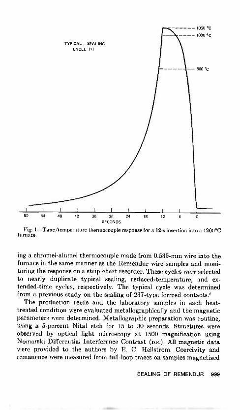
by an applied saturation field of 300 oersteds. All magnetic values pre-sented are the average of multiple samples. The laboratory sampleswere 2.5 cm in length, and the production samples were actual reedspossessing their characteristic geometry (Fig. 4). The reeds were mea-sured both as complete reeds with the search coil centered over thepaddle portion and also as dissociated paddles and shanks.
III. RESULTS AND DISCUSSION
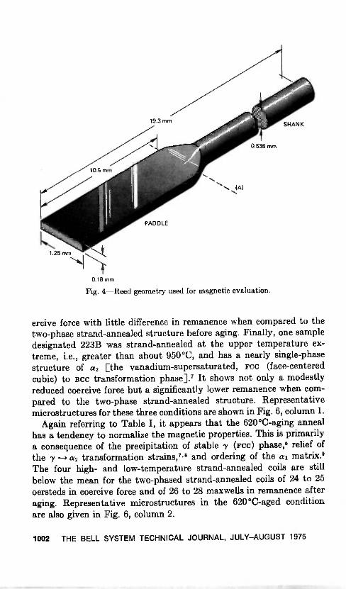
Microstructural comparisons and correlations were obtained onlongitudinal sections of the shanks. Figure 5 shows the microstructurespresent in a typical reed shank after sealing, at approximately 1 -mmincrements along its length. It is apparent that, in this case, beginningat the paddle end, approximately the first 5.5 mm have undergone astructural change. This represents approximately two-thirds of theshank length. This heat -affected region is substantially larger thanthat actually encompassed by the glass in the seal.
1000 THE BELL SYSTEM TECHNICAL JOURNAL, JULY-AUGUST 1975

EXTENDED - TIMECYCLE (3)
I I 1 I I I
60 54 48 42 36 30
SECONDS
24 18 12 6
1050 °C
Fig. 3-Time/temperature thermocouple response for a 25-s insertion into a 1200°Cfurnace.
3.1 Laboratory -simulated sealing -cycle exposures
To determine the significance of this structural change, the lab-oratory experiment utilizing various elevated -temperature exposureswas carried out. The magnetic -properties data for the 15 selected coilsare summarized in Table I. Of the 15 coils selected, 11 are consideredto possess a microstructure at least approximating a nearly equal dis-tribution of the two phases, al a2, in this duplex BCC structure.'This distribution is expected from an optimized -temperature strandanneal and quench.' In this strand -annealed state, these typical wiresindicate a coercive force of 41 to 47 oersteds and a remanence of 21to 23 maxwells for the specified measuring conditions. Three samplesdesignated 208B, 240B, and 268B were strand -annealed at the lowtemperature extreme, i.e., less than about 900°C, and have a nearlysingle-phase structure of al (Bcc). They have a significantly lower co -
SEALING OF REMENDUR 1001
0.18 mm
Fig. 4-Reed geometry used for magnetic evaluation.
ercive force with little difference in remanence when compared to thetwo-phase strand -annealed structure before aging. Finally, one sampledesignated 223B was strand -annealed at the upper temperature ex-treme, i.e., greater than about 950°C, and has a nearly single-phasestructure of «2 [the vanadium -supersaturated, FCC (face -centeredcubic) to BCC transformation phase].' It shows not only a modestlyreduced coercive force but a significantly lower remanence when com-pared to the two-phase strand -annealed structure. Representativemicrostructures for these three conditions are shown in Fig. 6, column 1.
Again referring to Table I, it appears that the 620°C -aging annealhas a tendency to normalize the magnetic properties. This is primarilya consequence of the precipitation of stable -y (FCC) phase,' relief ofthe 7 - a2 transformation strains,'," and ordering of the al matrix.'The four high- and low -temperature strand -annealed coils are stillbelow the mean for the two -phased strand -annealed coils of 24 to 25oersteds in coercive force and of 26 to 28 maxwells in remanence afteraging. Representative microstructures in the 620 °C -aged conditionare also given in Fig. 6, column 2.
1002 THE BELL SYSTEM TECHNICAL JOURNAL, JULY-AUGUST 1975
Arj
e:1.
.;e'l
.4 .4
11.6
.I
15i".
/4,
41*
cn I
1%, .
:1%
,
P-4)
A
11.
i101
..41
cst "
47-
4Li
j(.
9
Let
, 0 C5 z a) U 4.)
C.)
cn cn -Cf
a) a) "d C)
"73 43 4. 0 tit 0
0 E
C.)
-0.0 a)
ta0
Ocd C)
c.)
"C$ O
Ipc
3
b:05,wa
SE
ALI
NG
OF
RE
ME
ND
UR
1003

Table I - Magnetic properties of Remendur wire before andafter simulated sealing cycles 1, 2, and 3
He (oersteds)
SampleStrand -Anneal
StructureStrand -
AnnealedAged
620°C-3 hrTypical
Cycle (1)Low T
Cycle (2)Long t
Cycle (3)
205 T 2 phase 41.4 24.3 32.8 16.6 28.6205 B 2 phase 40.9 22.2 35.6 22.7 27.5208 B Primarily al 29.9 17.3 34.3 13.9 27.8218 T 2 phase 46.6 25.5 35.4 29.1218 B 2 phase 44.7 25.0 36.1 16.0 26.5223 T 2 phase 42.6 23.8 37.4 19.7 28.8223 B Primarily a2 35.5 22.7 33.0 14.2' 27.7'231 T 2 phase 45.4 25.6 38.5 16.9 25.9231 B 2 phase 47.3 27.3 38.5 18.3 28.9236 T 2 phase 38.5 24.3 37.1236 B 2 phase 43.5 26.4 36.3 14.5 26.3240 T 2 phase 44.6 25.8 37.3 17.1 28.3240 B Primarily al 23.0 19.0 37.3 13.9 29.2268 T 2 phase 46.7 27.0 38.5 17.8 27.4268 B Primarily al 21.0 19.0 37.0 29.5
On (maxwells
SampleStrand -Anneal
StructureStrand -
AnnealedAged
620°C-3 hrTypical
Cycle (1)Low T
Cycle (2)Long t
Cycle (3)
205 T 2 phase 22.2 27.2 16.3 21.9 11.1205 B 2 phase 22.3 23.2 18.1 24.2 11.3208 B Primarily al 22.1 21.4 16.5 20.6 11.0218 T 2 phase 22.9 27.9 17.3 12.9218 B 2 phase 22.6 27.5 18.2 22.6 11.8223 T 2 phase 22.3 25.2 19.1 21.8 12.2223 B Primarily az 17.3 25.2 15.1 9.3* 7.6*231 T 2 phase 22.8 28.3 20.2 22.9 11.3231 B 2 phase 22.9 28.4 20.2 24.6 13.4236 T 2 phase 21.9 27.7 19.6236 B 2 phase 22.7 26.6 19.1 19.5 12.0240 T 2 phase 22.7 25.7 19.0 23.0 11.4240 B Primarily al 20.6 20.8 19.5 19.3 12.2268 T 2 phase 23.1 27.4 20.6 22.9 11.2268 B Primarily al 20.3 21.2 19.6 11.9
Material : 2.90 weight percent V (i) T = front of coil, (ii) B = back of coil, (iii)H." = 300 oersteds, (iv) Values average of two or three samples, (v) Sample length= 2.5 cm.
' Aged at 515°C prior to elevated temperature exposure; 1.6 -cm sample length.
Samples were exposed to the typical -sealing cycle given in Fig. 1,which was based on a previous experimental evaluation of the time -temperature cycle experienced by a 52 -alloy reed in the sealing of atype 237 (nonlatching, Ni-Fe) reed contact.' This cycle creates anexposure to a peak temperature of 1050°C and temperatures in excess
1004 THE BELL SYSTEM TECHNICAL JOURNAL, JULY -AUGUST 1975

STRAND -ANNEALED 620°C -AGED
231T
He = 45.4 OR =22.8
Hc = 23.0 OR = 20.6
2238
Hc = 25.6 OR = 28.3
Hc = 19.0 OR = 20.8
Hc = 22.7 OR = 25.2
Fig. 6-Microstructures in strand -annealed and 620°C -aged conditions for two-phase (231T), primarily al -phase (240B), and primarily az-phase (223B) strand -annealed structures-etched 5 -percent nital, DIC, 1500X.
of 900°C for approximately 7 seconds. This exposure produces amarked increase in coercive force into the range of 33 to 38 oersteds anda drop in remanence to 15 to 20 maxwells (Table I) for all samples.Representative microstructures given in Fig. 7, column 1, indicatethat this change is a result of the material altering to the structuretypically produced by the 900 to 950°C strand -anneal.' That is, the7 (FCC) precipitates are dissolved and portions of the matrix return tothe high -temperature FCC phase and again undergo the FCC BCC
SEALING OF REMENDUR 1005
TYPICAL-SEALING REDUCED-TEMPERATURE EXTENDED-TIMECYCLE (3)CYCLE (1) CYCLE (2)
231T
iik.V*':":, .1.,i '.. -,.t.t:o'''\.;°1'tit' ..\ Ke...1, 0.41,
*.'4,"!': -' .i\'': '-* ' :-1-:::.
'4*-- -1*.** :I.C...' I ''Q'ttli7,-.- .1.,: -.` -k,c;A:,..14'
-, X./A` .'i'.i;t.',.t.i
'--.X .- ._
LVI. "it'q...,
.......
' %,!... V4.11V-";' t''''41.,,-;...1,.... \-:1 .. N*44., ..'!.n...:-..... t t . .'..),x t.. -zt.::. ":---..
Hc = 38.5 dR =20.2
Hc = 37.3 OR = 19.5
Hc = 33.0 OR = 15.1
Hc = 16.9 dR = 22.9
Hc = 13.9 dR = 19.3
He= 14.2* OR =9.3'
.
\A
' -!' !
Hc = 25.9 dR = 11.3
.
Hc = 29.2 OR = 12.2
Hc = 27.7* OR = 7.6*
*AGED AT 515°C; SAMPLE LENGTH = 1.6 cm
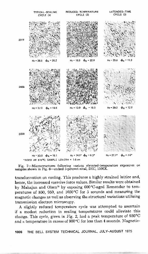
Fig. 7-Microstructures following various elevated -temperature exposures onsamples shown in Fig. 6-etched 5 -percent nital, DIC, 1500X.
transformation on cooling. This produces a highly strained lattice and,hence, the increased coercive force values. Similar results were obtainedby Mahaj an and Olsen" by exposing 600°C -aged Remendur to tem-peratures of 850, 950, and 1050°C for 5 seconds and measuring themagnetic changes as well as observing the structural variations utilizingtransmission electron microscopy.
A slightly reduced temperature cycle was attempted to ascertainif a modest reduction in sealing temperatures could alleviate thischange. This cycle, given in Fig. 2, had a peak temperature of 930°Cand a temperature in excess of 900°C for less than 4 seconds. Magnetic -
1006 THE BELL SYSTEM TECHNICAL JOURNAL, JULY-AUGUST 1975

properties results (Table I) show that the coercive force and remanenceare both reduced by this cycle. However, the remanence decrease issmall in all cases and, in general, those samples that had a two-phasestrand -annealed microstructure before aging and high temperatureexposure show a lesser decline in coercivity than the single-phasestrand -annealed structures. Microstructural observations (Fig. 7,column 2) indicate that these changes are a result of the beginning ofthe dissolution of the 7 (Fcc) precipitate. This cycle is sufficiently lowin temperature and time such that none of the matrix is returned toFCC structure at temperature and, hence, does not undergo the Fcc
Bcc transformation on cooling to markedly increase the magnetichardness as observed in cycle 1.
To clearly prove that a reversion to the strand -annealed structureduring sealing is the cause for the magnetic property changes observedin reeds,' an extended -time -at -temperature cycle was produced (Fig. 3).The peak temperature was maintained at 1050°C, but the time inexcess of 900°C was increased to 20 seconds. In all cases, the structuretotally converted to a single-phase a2 matrix (Fig. 7, column 3), whichis typical of a strand anneal at too high a temperature ( > 950 to975°C).° These structures may be compared to the initial structure ofcoil 223B in this experiment (Fig. 6, column 1), which was stated tobe a nearly -all -a2 matrix. This heat treatment produces an extremelyskewed hysteresis loop with a coercive force of 26 to 29 oersteds and agreatly reduced remanence to 11 to 13 maxwells (Table I) as measuredon 1 -inch samples. It is thus clear that very brief exposure to tempera-tures in excess of 900 to 1000°C can markedly alter the magneticproperties previously developed by the 600°C -aging heat treatmentin Remendur.
3.2 Analysis of production reeds
The results of the before -and -after glass -to -metal sealing analysis onactual production reeds (Table II) correlate well with the above ob-servations on the simulated -sealing temperature exposures. Listed arethe coercive force and remanence as measured on the complete reed,with search coil on the paddle, and also as measured on the dissociatedpaddles and shanks both before and after exposure to sealing (Experi-ment A). As was previously observed by others,' the major effect ofsealing is a marked increase in coercive force on the shank. In thisinstance, an average increase in the shank of about 6 oersteds from23.5 to 29.5 occurred. As expected, no change in the paddle portionwas observed, since it does not experience the peak temperature range.
The structural changes observed in the shanks of actual sealed reedsare very similar to those produced by the typical sealing cycle in theelevated -temperature -exposure experiments. The disappearance of the
SEALING OF REMENDUR 1007

Table II - Magnetic properties of Remendur reeds beforeand after glass/metal sealing
Experi-ment Samples Complete Reed -
search coil on paddle Shank Paddle
r610°C
He (oer.) OR(maxwells) He (oer.) R
(maxOwells) He (oer.) (maxwells)
A 4 Aged reed 27.4 (3) 21.5 (3) 23.6 (3) 5.9 (3) 28.4 (3) 10.0 (3)Sealed reed 29.7 (12) 19.3 (12) 29.0 (16) 6.7 (16) 28.7 (16) 10.0 (16)
B I Acceleratedspeed seal 28.3 (11) 21.6 (11) 25.9 (11) 6.1 (11) 28.9 (11) 10.3 (11)
reed -normal lamp
C
{Sealed
powerSealed reed -
reduced lamp
29.5 (6) 21.1 (6) 28.2 (6) 6.4 (6) 29.2 (6) 10.3 (6)
power 28.0 (6) 22.0 (6) 24.9 (6) 6.1 (6) 29.1 (6) 10.2 (6)
(i) H applied = 300 oersteds.(ii) Numbers in parentheses indicate sample size.
-y (Fcc) precipitate and return to the two-phase al a2 structure orall -a2 structure are apparent in Fig. 5.
The results from the reeds sealed by using the accelerated speedsealing (Experiment B) and with reduced lamp power (Experiment C)show an improvement. As can be noted in Table II, the coercivityincrease for the complete reed was smaller, and no drop in remanenceoccurred. The data on the dissociated shanks show that a coercivityincrease still occurred on these shanks, but it was markedly smallerthan that for the standard sealing operation. Metallographic resultsalso showed that a structural change had taken place but was confinedwithin a smaller percentage of the shank length. This probably ac-counts for the less drastically altered magnetic properties.
IV. SUMMARY AND CONCLUSIONS
The alteration of the magnetic properties of Remendur by the glass -to -metal sealing operation from those properties developed in thenominal 600 °C -aging anneal is real. This is a consequence of excessivetemperatures during the sealing operation causing a dissolving of the-y (Fcc) precipitate and a reversion of the structure back to that de-veloped by the typical 900 to 950°C strand anneal used in processingthe wire. With the present time/temperature sealing cycle used inproduction, the following more specific conclusions can be listed :
(i) From one-half to two-thirds of the shank length, beginning atthe paddle/shank transition region, is altered by the sealingoperation.
(ii) A significant increase in coercive force occurs in the shank.
1008 THE BELL SYSTEM TECHNICAL JOURNAL, JULY -AUGUST 1975

(iii) Laboratory results indicate that a significant drop in remanencealso occurs during elevated temperature exposures, which aresufficiently high to cause a reversion to the two-phase al a2or all -a2 structures.
(iv) Variations in the microstructure of 0.535 -mm wire from thestrand anneal have little effect on the subsequent structure andmagnetic properties changes during sealing.
A reduced -temperature sealing cycle holds some promise for minimizingthis change, but all 2.5- to 3.0 -percent vanadium Remendur alloys arelikely to exhibit this same behavior independent of vanadium contentor prior aging heat treatment. If this properties change is consideredunacceptable, a modification in the sealing cycle or a redesign of thecontact to account for this change are the most promising approaches,since the materials response cannot be altered.
V. ACKNOWLEDGMENTS
The authors express their appreciation to D. M. Sutter, P. W.Renaut, L. Herring, and K. Strauss for their cooperation in supplyingtheir data and samples to aid in this investigation. The efforts of E. C.Hellstrom in obtaining all the magnetic data cited in this investigationare also gratefully acknowledged. The excellent metallographic prep-aration provided by G. V. McIlhargie is noted, and, finally, the con-structive comments and usual thorough review of the manuscriptprovided by F. E. Bader are appropriately acknowledged.
REFERENCES
1. R. J. Gashler, W. A. Liss, and P. W. Renaut, "The Remreed Network: A Smaller,More Reliable Switch," Bell Laboratories Record, 51, No. 7 (July -August1973), pp. 202-207.
2. D. M. Sutter and P. W. Renaut, unpublished work, 1973.3. T. Kitazawa, T. Oguma, and T. Hara, "Miniature Semihard Magnetic Dry
Reed Switch," Proc. 19th National Relay Conference, Oklahoma StateUniversity, 1971, pp. 12-1-12-9.
4. M. R. Pinnel and J. E. Bennett, "The Metallurgy of Remendur: Effects ofProcessing Variations," B.S.T.J., 52, No. 8 (October 1973), pp. 1325-1340.
5. J. E. Bennett and M. R. Pinnel, "Aspects of Phase Equilibria in Fe/Co/2.5 to3.0% V Alloys," J. of Material Sci., 9, No. 7 (July 1974), pp. 1083-1090.
6. T. F. Strothers, "Temperature Measurement of 237 Sealed Contact DuringManufacture," unpublished work, 1971.
7. S. Mahajan, M. R. Pinnel, and J. E. Bennett, "Influence of Heat Treatments onMicrostructures in an Fe -Co -V Alloy," Met. Trans., 5, No. 6 (June 1974),pp. 1263-1272.
8. M. R. Pinnel and J. E. Bennett, "Correlation of Magnetic and MechanicalProperties with Microstructure in Fe/Co/2-3 pct V Alloys," Met. Trans., 5,No. 6 (June 1974), pp. 1273-1283.
9. A. T. English, "Long Range Ordering and Domain Coalescence Kinetics inFe -Co -2V," Trans. AIME, 236, No. 1 (January 1966), pp. 14-20.
10. S. Mahajan and K. M. Olsen, "An Electron Microscopic Study of the Origin ofCoercivity in an Fe -Co -V Alloy," unpublished work, 1974.
SEALING OF REMENDUR 1009

.... ., K, .i:i.NiY. MrYe i:,
Copyright © 1975 American Telephone and Telegraph CompanyTHE BELL SYSTEM TECHNICAL JOURNAL
Vol. 54, No. 6, July -August 1975Printed in U.S.A.
A Multibeam, Spherical -Reflector SatelliteAntenna for the 20- and 30-GHz Bands
By R. H. TURRIN(Manuscript received November 18, 1974)
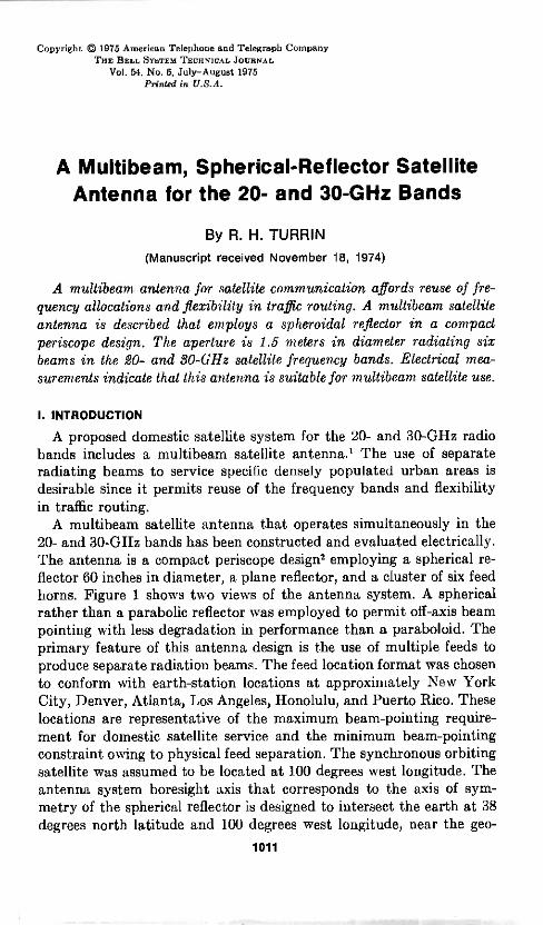
A multibeam antenna for satellite communication affords reuse of fre-quency allocations and flexibility in traffic routing. A multibeam satelliteantenna is described that employs a spheroidal reflector in a compactperiscope design. The aperture is 1.5 meters in diameter radiating sixbeams in the 20- and 30-GHz satellite frequency bands. Electrical mea-surements indicate that this antenna is suitable for multibeam satellite use.
I. INTRODUCTION
A proposed domestic satellite system for the 20- and 30-GHz radiobands includes a multibeam satellite antenna.' The use of separateradiating beams to service specific densely populated urban areas isdesirable since it permits reuse of the frequency bands and flexibilityin traffic routing.
A multibeam satellite antenna that operates simultaneously in the20- and 30-GHz bands has been constructed and evaluated electrically.The antenna is a compact periscope design' employing a spherical re-flector 60 inches in diameter, a plane reflector, and a cluster of six feedhorns. Figure 1 shows two views of the antenna system. A sphericalrather than a parabolic reflector was employed to permit off -axis beampointing with less degradation in performance than a paraboloid. Theprimary feature of this antenna design is the use of multiple feeds toproduce separate radiation beams. The feed location format was chosento conform with earth -station locations at approximately New YorkCity, Denver, Atlanta, Los Angeles, Honolulu, and Puerto Rico. Theselocations are representative of the maximum beam -pointing require-ment for domestic satellite service and the minimum beam -pointingconstraint owing to physical feed separation. The synchronous orbitingsatellite was assumed to be located at 100 degrees west longitude. Theantenna system boresight axis that corresponds to the axis of sym-metry of the spherical reflector is designed to intersect the earth at 38degrees north latitude and 100 degrees west longitude, near the geo-
1011

PLANE REFLECTORPLATE GLASS MIRROR
183 x 254 cm
FEEDS
11,
1\\\'k,
APERTUREREGION -
PLAN VIEW
FRONT VIEW
-- f = 120 cm ---
SPHERICAL'SURFACE
REFLECTOR
Fig. 1-Multibeam antenna.
graphic center of the contiguous United States. With these geo-graphical constraints, the maximum beam -pointing angle off boresightis about ±6.5 degrees in the east -west direction to include Honoluluand Puerto Rico.
Parameters of chief interest in the electrical evaluation of thisantenna system are isolation between beams, absolute pointing ac-curacy of beams, coupling between feeds, and performance degradationbecause of feed -cluster blockage. Although these parameters may beevaluated analytically, the last one is especially difficult to analyze.For this reason and to demonstrate the others, a laboratory model wasconstructed and measurements were made.
1012 THE BELL SYSTEM TECHNICAL JOURNAL, JULY-AUGUST 1975
II. CONSTRUCTION
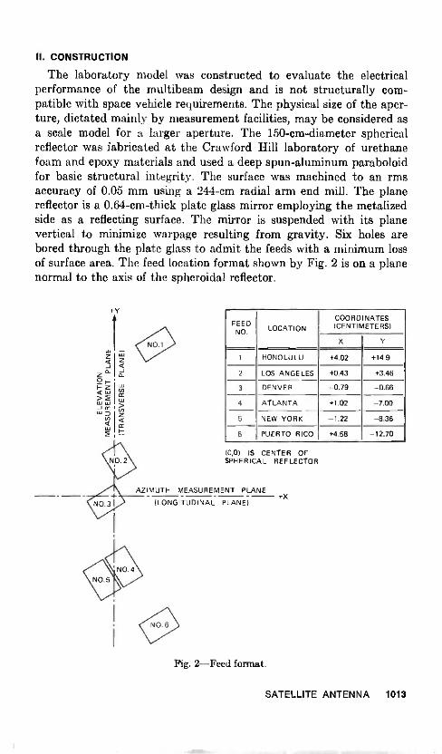
The laboratory model was constructed to evaluate the electricalperformance of the multibeam design and is not structurally com-patible with space vehicle requirements. The physical size of the aper-ture, dictated mainly by measurement facilities, may be considered asa scale model for a larger aperture. The 150 -cm -diameter sphericalreflector was fabricated at the Crawford Hill laboratory of urethanefoam and epoxy materials and used a deep spun -aluminum paraboloidfor basic structural integrity. The surface was machined to an rmsaccuracy of 0.05 mm using a 244 -cm radial arm end mill. The planereflector is a 0.64 -cm -thick plate glass mirror employing the metalizedside as a reflecting surface. The mirror is suspended with its planevertical to minimize warpage resulting from gravity. Six holes arebored through the plate glass to admit the feeds with a minimum lossof surface area. The feed location format shown by Fig. 2 is on a planenormal to the axis of the spheroidal reflector.
+Y
FEEDNO. LOCATION
COORDINATES(CENTIMETERS)
X Y
1 HONOLULU +4.02 +14.9
2 LOS ANGELES +0.43 +3.46
3 DENVER -0.79 -0.66
4 ATLANTA +1.02 -7.00
5 NEW YORK -1.22 -8.36
6 PUERTO RICO +4.58 -12.70
(0,0) IS CENTER OFSPHERICAL REFLECTOR
AZIMUTH MEASUREMENT PLANE
(LONGITUDINAL PLANE)
Fig. 2-Feed format.
+x
SATELLITE ANTENNA 1013

The feed horns were designed for dual -frequency operation withlinear polarization. The polarization for the 20- and 30-GHz bandsare orthogonal. Figure 3 shows details of the feed horn employing thinconductive fins that redefine the electrical aperture for the 30-GHzband. Since the 20-GHz polarization is normal to the fins, the feed -horn walls define the aperture for this band. By using the fins toselectively control the feed aperture size, the radiation patterns atboth 20 and 30 GHz are more nearly the same, resulting in optimumillumination for the spheroidal reflector at both frequencies. Figures 4and 5 show feed radiation patterns at measurement frequencies of 19and 30.2 GHz.
The axis of each feed was aligned parallel to the axis of the spheroidalreflector aperture and the feed -phase centers were arranged in a singleplane located 120 cm from the center of the spheroidal reflector.Measurements on positioning of a single movable feed showed thatthere is no significant difference in radiation characteristics of theantenna system for the off -axis beam -pointing directions under con-sideration with the feed axis oriented (i) along a radial direction fromthe center of curvature of the spheroidal surface, (ii) parallel to theaxis, or (iii) directed toward the center of the spheroidal reflector tobalance the amplitude distribution. Parallel mounting of the feed axesgreatly simplifies the feed -line structure. It was also found that arrang-ing the phase centers in a plane rather than in the optimum spheroidalfocal surface produces an error in focal length of less than X/2 at 30GHz with little effect on the gain or radiation characteristics of thesystem.
--- -3.82 cm ---
1.02 cm
SQUARE 'FLANGE
-- -3.82 cm-- -
1.91 cm
BRASS FINS 1 -
SOLDERED INTO SLOTSIN HORN WALLS
1
/F
cm
\N I
N i
N.N1NN
N N I
N 'N N
3.061cm
\ \I
\ /N/ \ N
---I-
I
i
POLARIZATION ORIENTATIONREFERENCED TO APERTURE
30 GHz
20 GHz * a
Fig. 3-Linearly polarized feed horn, dual frequency (17.7-20.2 GHz and 27.5-30.0 GHz).
1014 THE BELL SYSTEM TECHNICAL JOURNAL, JULY -AUGUST 1975

ANGLE IN DEGREES10 0 10
20 0
5
10
15
20
E -PLANE
25
REFLECTOR30 EDGE
90
Fig. 4-Radiation patterns of the finned feed horn at 19.0 GHz.
The polarization orientations of the feeds were mandated by thephysical constraint of the feeds in New York City (feed 5) and Atlanta(feed 4) feeds. These two feeds were parallel -polarized and arrangedat a skew angle with respect to the measuring plane to achieve aminimum physical spacing. The remaining feeds were cross -polarizedwith their adjacent neighbors for minimum electrical coupling. Thefeed locations shown in Fig. 2 were necessary to achieve the desiredbeam -pointing angles for the various earth -station locations.
III. MEASUREMENTS
Electrical evaluation of the multibeam antenna was conducted atthe Holmdel radio range. A variation was found of incident field overthe measurement aperture of no greater than ±0.75 dB for either 19or 30 GHz, the measurement frequencies used.
SATELLITE ANTENNA 1015

ANGLE IN DEGREES10 0 10
REFLECTOR30 EDGE
ANGLE IN DEGREES10 0 10
Fig. 5-Radiation patterns of the finned feed horn at 30.0 GHz.
3.1 Beam pointing
Beam -pointing accuracy is important in the design of a satellitesystem. Measurement of pointing accuracy for each of the six beamswas accomplished by first mechanically measuring the location of eachfeed phase center relative to the axis of the spheroidal reflector (bore-
sight axis) and in the X -Y plane (Fig. 1). Alignment of the boresightaxis with the radio source was done by optical sighting. All measure-ments of beam pointing were made using synchro-type readouts withan accuracy of 0.05 degree. Angular measurements are in essentiallyan orthogonal coordinate system for the elevation -over -azimuthmount.
Table I shows all the measured beam -pointing data, together withcomputed data based on feed location, and the pointing errors. Thefeeds are numbered as in Fig. 2. Since the half -power beamwidth of
1016 THE BELL SYSTEM TECHNICAL JOURNAL, JULY-AUGUST 1975

Table I - Measured and computed beam -pointing errors
FeedNo.
Freq.(GHz)
Measuredar
(Degrees)
Computed0:
(Degrees)
PointingError
(Degrees)
Measured8
(Degrees)
Computed0
(Degrees)
PointingError
(Degrees)
19.0 -1.05 -0.08 +6.82 -0.081
Hon. 30.2 -1.71-1.87
+0.16 +7.28+6.90
+0.38
219.0 -0.35
-0.20-0.15 +1.50
+1.61-0.11
L.A. 30.2 -0.15 +0.05 +1.75 +0.14
19.0 +0.20 -0.17 -0.45 -0.143 +0.37 -0.31
Den. 30.2 +0.45 +0.08 -0.30 +0.01
19.0 -0.58 -0.10 -3.44 -0.194 -0.48 -3.25
Atl. 30.2 -0.40 +0.08 -3.40 -0.15
19.0 +0.35 -0.22 -4.17 -0.275 +0.57 -3.90
N.Y. 30.2 +0.56 -0.01 -4.08 -0.18
19.0 -2.19 -0.07 -6.14 -0.256 -2.12 -5.89
P.R. 30.2 -2.05 +0.07 -6.15 -0.26
each beam at both 19 and 30 GHz is about 0.65 degree, the maximumerror encountered in these measurements was about one-half beam -width. Considering the readout accuracy, mechanical errors in thestructure, and boresight errors, these results are remarkably con-sistent; the antenna beams point in the intended directions.
3.2 Beam coupling
Beam coupling is a measure of the signal level in one specified beamwhen another beam is aimed toward the source. It is also a measure ofthe interference between any two particular ground stations. Theradiation characteristics of each beam for specific off -axis angles specifythe coupling. Measured coupling for all combinations of beams ex-cept the New York City -Atlanta combination was found to be lessthan -35 dB. In that case, the angular separation in the beams isonly 1.2 degrees and the coupling is approximately -20 dB. The datawere measured at specific incremental frequencies over the 2500 -MHzband at both 20 and 30 GHz.
The beam coupling is strongly dependent on exact pointing direc-tions and can be greatly improved by slight misalignment of the mainbeams. It may, therefore, be an engineering expedience to suffer aslight degradation in gain by beam misalignment to improve theisolation.
3.3 Radiation patterns
Studies of the radiation characteristics of this antenna with a singlehorn feed were made prior to installation of the six -feed cluster. These
SATELLITE ANTENNA 1017

measurements were made to determine the effects of illumination onbeams pointed off -axis. Figure 6 gives measured values of relativegain and first side lobes with off -axis pointing. The asymmetric il-lumination with off -axis pointing produces an effect similar to comaaberration in which the first side lobe levels become increasingly un-balanced. The side lobe nearest the axis of the antenna system is alwaysthe higher in level, as expected.
The gain degradation for maximum off -axis pointing is a modest 1dB at 19 GHz. At 30 GHz, the extrapolated degradation is approxi-mately 2 dB. Representative measured far -field radiation patterns forthe single feed are shown by Figs. 7 and 8. These are principal planemeasurements, that is, patterns taken with a single feed whose polariza-tion orientation is parallel with the measurement plane; they show thetypical far -side -lobe behavior of this type of antenna.
Figures 9 and 10 are far -field radiation patterns at 19.0 GHz forfeeds 1 and 3, when all other feeds are in place and terminated. Theseare representative of the maximum and minimum off -axis pointing.Figures 11 and 12 are for the same feeds at 30.2 GHz. These patternsillustrate the off -axis asymmetric radiation characteristics; the effect
CO
co
wO
2
- / -15
30 GHz
-20
cc
-25 19 GHz
-300 1 2 3 4 5
ANGLE OFF AXIS IN DEGREES
Fig. 6-Single-feed measurements of off -axis performance.
afr
GAIN
FIRST SIDE LOBE LEVELS
00'for
-.0-
----- - 19
A
'30 GHz
6
1018 THE BELL SYSTEM TECHNICAL JOURNAL, JULY-AUGUST 1975
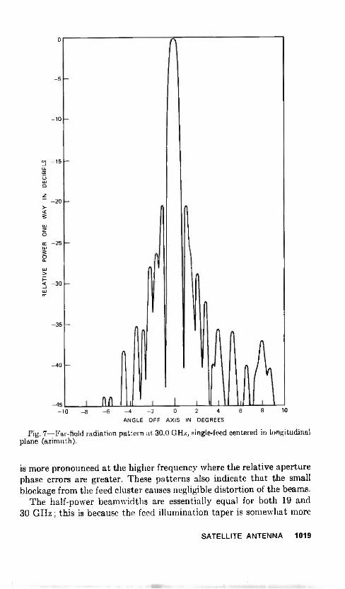
-10
-15
-20
-25
-30
-35
-40
-45-10
1111
-8 -6 -4 -2 0 2
114 6
ANGLE OFF AXIS IN DEGREES
8 10
Fig. 7-Far-field radiation pat tern at 30.0 GHz, single -feed centered in longitudinalplane (azimuth).
is more pronounced at the higher frequency where the relative aperturephase errors are greater. These patterns also indicate that the smallblockage from the feed cluster causes negligible distortion of the beams.
The half -power beamwidths are essentially equal for both 19 and30 GHz; this is because the feed illumination taper is somewhat more
SATELLITE ANTENNA 1019

-10
-15
-20
-25
-30
-35
-40
-45
4°
AI Al A
-6 -4 -2 0 2 4 6 8 10 12 14
ANGLE OFF AXIS IN DEGREES
Fig. 8-Far-field radiation pattern at 30.0 0Hz, single -feed offset in longitudinalplane.
severe at 30 GHz and because the reflector surface errors cause moredegradation at the higher frequency.
3.4 Gain
Absolute gain measurements shown in Fig. 13 corroborate thepattern measurements; the gain falls off faster with off -axis pointing
1020 THE BELL SYSTEM TECHNICAL JOURNAL, JULY-AUGUST 1975

-10
-J-20
Li,- -25
-30
-35
-40 I-6 -4 -2 0 2
ELEVATION ANGLEIN DEGREES
FEED NO. 319.0 GHz
RADIATION PATTERNS
fli.4 -4 0
AZIMUTH ANGLEIN DEGREES
Fig. 9-Feed 3, 19.0 -GM radiation patterns.
4 6
at 30 GHz than at 19 GHz. The plotted values in Fig. 13 show therelative gain measured for each feed. These data are consistent withsingle feed measurements where off -axis gain degradation was some-what more at 30 GHz than at 19 GHz. The aperture efficiency for thefeed nearest center, No. 3, is 54 percent at 19.0 GHz and 35.5 percentat 30.2 GHz.
3.5 Reflection coefficient
The magnitude of the reflection coefficient over each frequency bandwas measured at each feed port. The maximum value is -18 dB typi-
SATELLITE ANTENNA 1021
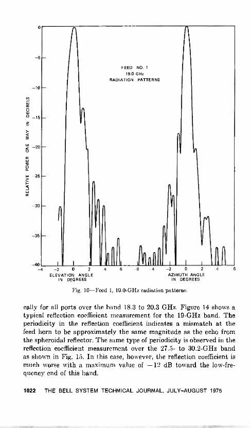
-10
-15
-20
-25
-30
-35
-40
FEED NO. 1
19.0 GHz
RADIATION PATTERNS
-4 -2 0 2
ELEVATION ANGLEIN DEGREES
6 -6 -4 -2 0 2
AZIMUTH ANGLEIN DEGREES
Fig. 10-Feed 1, 19.0-GHz radiation patterns.
cally for all ports over the band 18.3 to 20.3 GHz. Figure 14 shows atypical reflection coefficient measurement for the 19-GHz band. Theperiodicity in the reflection coefficient indicates a mismatch at thefeed horn to be approximately the same magnitude as the echo fromthe spheroidal reflector. The same type of periodicity is observed in thereflection coefficient measurement over the 27.5- to 30.2-GHz bandas shown in Fig. 15. In this case, however, the reflection coefficient ismuch worse with a maximum value of - 12 dB toward the low -fre-quency end of this band.
1022 THE BELL SYSTEM TECHNICAL JOURNAL, JULY-AUGUST 1975
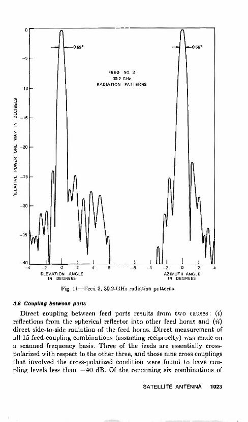
FEED NO. 330.2 GHz
RADIATION PATTERNS-10
-15
-20
-25
-30
-35
0.68°
-40 II I I I t I 11
-4 -2 0 2 4 -6 -4 -2 0 2 4
ELEVATION ANGLEIN DEGREES
AZIMUTH ANGLEIN DEGREES
Fig. I1-Feed 3, 30.2-GHz radiation patterns.
3.6 Coupling between ports
Direct coupling between feed ports results from two causes : (1)
reflections from the spherical reflector into other feed horns and (ii)direct side -to -side radiation of the feed horns. Direct measurement ofall 15 feed -coupling combinations (assuming reciprocity) was made ona scanned frequency basis. Three of the feeds are essentially cross -polarized with respect to the other three, and those nine cross couplingsthat involved the cross -polarized condition were found to have cou-pling levels less than -40 dB. Of the remaining six combinations of
SATELLITE ANTENNA 1023

-10
-15
-20
-25
-30
-35
-40
0.59°
FEED NO. 1
30.2 GHz
RADIATION PATTERNS
-4 -2 0 2 4 6 -6 -4 -2 0 2 4 6
ELEVATION ANGLE AZIMUTH ANGLEIN DEGREES IN DEGREES
Fig. 12-Feed 1, 30.2-GHz radiation patterns.
coupling for each frequency band, the worst case is for the adjacentfeeds 4 and 5 (New York -Atlanta), which show values of -24 dB at20 GHz and -26 dB in the 30-GHz band. All others show couplingless than -28 dB, consistent with reflection coupling from the spheri-cal surface alone. All unused ports were terminated during thesemeasurements.
IV. CONCLUSIONS
Measurements on a compact spherical periscope antenna indicatethat this design is suitable as a multibeam satellite antenna for the
1024 THE BELL SYSTEM TECHNICAL JOURNAL, JULY-AUGUST 1975

0
(13-1
.3W -1.0(.7)
z
z -2.0
0
-1.0
-2.0
- NO. 2NO. 3
NO. 5
NO. 4
30.2 GHz DATA
NO. 1
NO. 6
NO. 3- NO. 2 NO. 4
NO. 5
FRE-QUENCYIN GHz
MEASURE-MENTIN dB
AREA GAINIirD, X )2IN dB
GAIN BELOWAREAIN dB
19.0 47.01'0.5 49.67 -2.7
30.2 49.210.5 53.67 -4.5
19.0 GHz DATA
NO. 6
NO. 1
0 2 4 6 8 10 12
RADIAL FEED DISPLACEMENT OFF AXIS IN cm14 16
Fig. 13-Absolute gain measured at feed port 3 by standard gain horn techniques.
10
-15
-20
-25
-30
-4018.0
FEED PORT NO.4REFLECTION COEFFICIENT
REFLECTED LEVEL
I I .
18.5 19.0 19.5
FREQUENCY IN GHz
Fig. 14-Feed port 4, reflection coefficient.
20.0 20.5
SATELLITE ANTENNA 1025
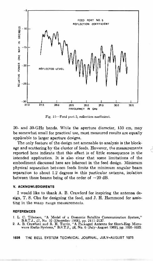
-5
FEED PORT NO. 5REFLECTION COEFFICIENT
-20
-25
-3027.0 27.5 28.0 28.5 29.0 29.5
FREQUENCY IN GHz
Fig. 15-Feed port 5, reflection coefficient.
30.0 30.5
20- and 30-GHz bands. While the aperture diameter, 150 cm, maybe somewhat small for practical use, most measured results are equallyapplicable to larger aperture designs.
The only feature of the design not amenable to analysis is the block-age and scattering by the cluster of feeds. However, the measurementsreported here indicate that this effect is of little consequence in theintended application. It is also clear that some limitations of theembodiment discussed here are inherent in the feed design. Minimumphysical separation between feeds limits the minimum angular beamseparation to about 1.2 degrees in this particular antenna, isolationbetween these beams being of the order of - 20 dB.
V. ACKNOWLEDGMENTS
I would like to thank A. B. Crawford for inspiring the antenna de-sign, T. S. Chu for designing the feed, and J. H. Hammond for assis-ting in the many range measurements.
REFERENCES
1. L. C. Tillotson, "A Model of a Domestic Satellite Communication System,"B.S.T.J., 47, No. 10 (December 1968), pp. 2111-2137.
2. A. B. Crawford and R. H. Turrin, "A Packaged Antenna for Short -Hop Micro-wave Radio Systems," B.S.T.J., 48, No. 6 (July -August 1969), pp. 1605-1622.
1026 THE BELL SYSTEM TECHNICAL JOURNAL, JULY -AUGUST 1975
Copyright © 1975 American Telephone and Telegraph CompanyTHE BELL SYSTEM TECHNICAL JOURNAL
Vol. 54, No. 6, July-August 1975Printed in U.S.A.
Polarization -Independent, MultilayerDielectrics at Oblique Incidence
By A. A. M. SALEH(Manuscript received January 6, 1975)
This paper gives solutions for multilayer dielectrics that yield polariza-tion -independent operation at a given angle of incidence and at a givenfrequency. An exhaustive analysis is given for symmetric three -layerdielectrics surrounded by the same medium. Special solutions are alsogiven for symmetric multilayer dielectrics with more than three layerssurrounded by the same medium and for multilayer dielectrics surroundedby different media. Rules are presented for obtaining new polarization -independent solutions by cascading given solutions. Finally, for the purposeof demonstration and comparison of various solutions, different designexamples are carried out for polarization -independent 3 -dB beam splittersto operate at millimeter wavelengths.
I. INTRODUCTION
The state of polarization of a plane wave will, in general, be changedupon transmission through or reflection by a multilayer dielectric atoblique incidence. The reason for this depolarization is that the twoeigenmodes of polarization, E -field perpendicular to the plane of inci-dence and E -field parallel to the plane of incidence, generally havedifferent reflection coefficients and different transmission coefficients.This is not desirable in many applications. For example, such depolari-zation could cause crosstalk in dual -polarization optical or quasi -optical components such as interference filters,' directional couplers2-5and diplexers,6 or mode conversion in beam-splitter-type hybrids7.5in oversized waveguides.
This paper provides solutions for multilayer dielectrics whose reflec-tion and transmission coefficients are independent of the state ofpolarization of the incident wave at a given angle of incidence and agiven frequency. Compromising the degree of polarization indepen-dence to allow for a broader bandwidth of operation or for variationsin the angle of incidence, even though desirable in many practical ap-plications, is not discussed.
1027

The paper is primarily concerned with symmetric, multilayer di-electrics surrounded by the same medium. However, the case of differ-ent input and output media and antireflective coatings is also dis-cussed. Some of the results given in this paper have been previouslyreported by Kard,8 Baumeister,' and Rabinovitch and Pagis.'" Theirwork is referred to in appropriate places in the text.
There are other types of structures, besides the ones reported in thispaper, that can give polarization -independent operation at obliqueincidence. For example, artificial or natural anisotropic dielectriclayers or metallic -wire meshes with rectangular, rather than square,cells can, in principle, be constructed to achieve this effect.
II. BASIC EQUATIONS
Consider n adjacent isotropic dielectric layers of infinite transverseextent having relative dielectric constants of Ely E2y y en and uniformthicknesses of d1, d2, , do inserted in a medium of a relative dielectricconstant Er. Define
Ki ----- ei/ er, i= 1, 2, , n (1)
as the normalized dielectric constants of the layers. Let a uniformplane wave propagating in the medium be incident at an angle 0 on thelayers as shown in Fig. 1. The incident, transmitted and reflected waveswill have the same state of polarization if the E -field is perpendicular
a
Fig. 1-n -layer dielectric inserted in a medium of a relative dielectric constant Er.The subscript h refers to the h -mode (E -field perpendicular to plane of incidence),and e refers to the e -mode (E -field parallel to plane of incidence).
1028 THE BELL SYSTEM TECHNICAL JOURNAL JULY-AUGUST 1975

to the plane of incidence (h -mode), or if the E -field is parallel to theplane of incidence (e -mode). To calculate the transmission and reflec-tion coefficients for the h- and e -modes, one can represent each layerby an equivalent transmission line." '2 The impedance of the linerepresenting the ith layer normalized to that of the line representingthe medium in which the layers are inserted is
Zi = Zih = cos 0/(Ki - sin2 0)i (2a)
for the h -mode, and
Zi = Zie = (Ki - sin2 0)1/(Ki cos 0) (3a)
for the e -mode. The corresponding electrical length is
ctsi = (27r/Xo)di(Ki - sin2 0)i (4a)
for both modes; A0 being the free -space wavelength. If Ki < sin2 0, i.e.,the total reflection condition is satisfied at the boundary of the ithlayer, then the square root of (Ki - sin2 0) is imaginary and one canwrite
Zoi = (2b)
Zie = (3b)
cki = (4b)
where Xih, Xie, and «i are positive, real quantities. In this case, cou-pling is accomplished across that layer by an evanescent wave.
The normalized ABCD matrix corresponding to the ith layer is
Mi =cos (ki j sin 4jZi
j sin 4,i/Zi cos oi(5)
The overall, normalized ABCD
A jB
matrix of the n layers is
jC D= MiM2 Mn (6)
The reason for the j in the off -diagonal terms of the matrix of eq. (6)is that A, B, C, and D will be real quantities if the system is lossless.Henceforth, this will be assumed to be the case.
It is worth noting that reciprocity requires that
AD -I- BC = 1, (7)
and that for a symmetric structure
A = D. (8)
MULTILAYER DIELECTRICS 1029
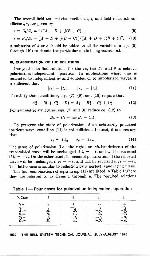
The overall field transmission coefficient, t, and field reflection co-efficient, r, are given by
t --.= EVEi = 2/[A -I- D + j(B + C)], (9)
r --- Er/Et = [A -D + j(B - C)]/[24. ± D + j(B + C) ]. (10)
A subscript of h or e should be added to all the variables in eqs. (5)through (10) to denote the particular mode being considered.
III. CLASSIFICATION OF THE SOLUTIONS
Our goal is to find solutions for the K's, the d's, and 0 to achievepolarization -independent operation. In applications where one isrestricted to independent h- and e -modes, or to unpolarized waves, itis sufficient that
IthI = Itel, IrhI = ire'. (11)
To satisfy these conditions, eqs. (7), (9), and (10) require that
A?, ± Bh + cg + Dg = Al + Be + oe + D2e. (12)
For symmetric structures, eqs. (7) and (8) reduce eq. (12) to
Bh - Ch = ±(Be - Ce). (13)
To preserve the state of polarization of an arbitrarily polarizedincident wave, condition (11) is not sufficient. Instead, it is necessarythat
th = Etej rh = ±re. (14)
The sense of polarization (i.e., the right- or left-handedness) of thetransmitted wave will be unchanged if th = +te and will be reversedif th = -te. On the other hand, the sense of polarization of the reflectedwave will be unchanged if rh = -re and will be reversed if rh = -Fr..The latter case is similar to reflection by a perfect, conducting plane.
The four combinations of signs in eq. (11) are listed in Table I wherethey are referred to as Cases 1 through 4. The required relations
Table I - Four cases for polarization -independent operation
\Case 1 2 3 4
th=rh=Ah=Bh=Ch=Dh=
t,rA.B.C.D.
t,-r,
D,C.B.A,
-t,r,
-A,-B.-C,-D,
-t,-r,-D,-C.-B,-A,
1030 THE BELL SYSTEM TECHNICAL JOURNAL, JULY-AUGUST 1975

between A,,, Bh, C,,, D,, and A Be, Ce, De to satisfy each of these casescan be deduced from eqs. (9) and (10) and are also given in Table I.
In addition to classifying the solutions in the manner of Table I,another classification based on the numerical values of the K's is useful.To be concise, let Kmin be the smallest value of the K's and let it be atthe mth layer, i.e.,
Kmin -=- min (K1, K2, , K rt) = Km. (15)
If Kmin 1, then none of the K's is smaller than unity and the solutioncan be realized by dielectric layers, ei 1, inserted in air, Er = 1. Thiswill be referred to as a Type A solution. On the other hand, if Kmin < 1,the surrounding medium can no longer be air since this would requirethat at least en, be less than unity (recall that m is the layer with thesmallest value of K) j thus, a dielectric -prism realization as shown inFig. 2 is necessary. In this case, the mth layer can be an air separation
= 1, and thus, from eq. (1)
Ei = K di( m in 1, Er = 1 /K m in > 1. (16)
The prism realization will be referred to as a Type B solution when1 > Kmin sin2 0, and a Type C solution when Kmin < 51112 O. The dis-
MATCHING LAYERS,
c./rEN \\I -Os//
CO'i.<Cs
0..csEn
N1%,o",e
-r
Fig. 2-A prism realization having the mth layer (the layer with the smallestdielectric constant) made of an air separation. Note that Km = Kmin < 1. Matchinglayers are required at the external surfaces of the prisms.
MULTILAYER DIELECTRICS 1031

Table II -The three types of solutions
Type A B C
Condition Ktnin '' 1 sine 0 < Kinin < 1 Kmin < sin2 0
Description Dielectric slabs inair (er = 1) ispossible.
Prism realization(er > 1) isnecessary. Noevanescentwaves.
Prism realization(er > 1) is neces-sary. Evanescentwaves exist.
tinction is made because in a Type C solution, the condition for totalreflection is satisfied at the boundary of the mth layer and couplingacross that layer is accomplished by an evanescent wave, as mentionedin Section II. This is not the case for a Type B solution. Table IIsummarizes the conditions for the three types of solution.
Dielectric -prism devices have been used for many optical"," andquasi-optica12-535-18 applications. When the total reflection condition issatisfied, Type C realization, the device is often said to be of the frus-trated -total -reflection type.
Fresnel reflections at the outer surfaces of the prisms might causeundesirable effects.19 However, this can be avoided by matching eachof these surfaces by the familiar X/4 transformer, or by othermeans.2,20-22 In any case, for the purpose of this paper, the method ofmatching should be independent of the state of polarization of theincident wave. Thus, Brewster angle matching17," would not be suit-able here.
In the remainder of the paper, a combined reference to the fourcases of Table I and the three types of Table II is adopted. For ex-ample, Case 1A refers to Case 1 of Table I and Type A of Table II.
IV. SINGLE -LAYER SOLUTIONS
It can be shown by using the procedure outlined in Section II thatno solution exists for a single layer to satisfy any of the four casesindicated in Table I. However, it is possible to satisfy the weaker con-dition given in eq. (11) by requiring that
K1 = El/ er = sin2 0/(1 + cos2 0), (17)
where the symbols are defined in Fig. 1 with n = 1. Substituting eq.(12) into eqs. (2) through (10), one obtains
1h = 1e, rh = (18)
where the asterisk denotes complex conjugation.
1032 THE BELL SYSTEM TECHNICAL JOURNAL, JULY-AUGUST 1975

It is clear from eq. (17) that Ki < sine 0 and, hence, from Table II,the solution is of Type C, and a prism realization is necessary.
It is interesting to note that condition (17) is independent of thethickness, d1, of the layer. Thus, varying d1 will change the reflectionand transmission coefficients without affecting the polarization inde-pendence. If R = I r12 is the required power reflection coefficient, theneqs. (17) and (2) through (10), with n. = 1, give
d1 = [X./(20T(1 KI)/(1 -X sinh-1 { 2[KiR/ (1 - R)]1/ (1 + Ki)}. (19)
A continuous variation of d1, and hence of R, can be accomplishedmost conveniently if the layer is simply an air separation, el = 1. Inthis case, if the angle of incidence is 0 = 45°, which is convenient formechanical considerations, eq. (17) requires the dielectric constantof the prisms to be er = 3. On the other hand, if the prisms were madeof polystyrene, er = 2.54, eq. (17) requires that 0 = 48.73°.
V. SYMMETRIC THREE -LAYER SOLUTIONS
It was mentioned in the previous section that no single -layer solutionexists that satisfies any of the four cases of Table I. The same is alsotrue for two layers. On the other hand, one can satisfy any of the fourcases with three or more layers. In this section, we give all the solutionsfor symmetric three -layer structures, i.e.,
K3 = Kl, d3 = d1. (20)
Even though unsymmetric three -layer structures can have polariza-tion -independent solutions, they will not be discussed here because ofthe algebraic complexities involved.
Using the terminology of Section II, it can be shown that thenormalized ABCD parameters of a symmetric three -layer structureare given by
A = D = cos 4)2 cos (201) 1[Z1/Z2 Z2/Z1i sin 02 sin (201) (21)
B = Z1 cos 02 sin (201) + Z2 sin 02 cos' 01- [ZUZ2] sin 02 sin2 01 (22)
C = ZF' cos 02 sin (200 Z.T' sin 4,2 cos' csi- [Z2/Z;] sin 42 sin2 ch. (23)
Combining these equations with eqs. (2) through (4), (9), and (10),one can obtain solutions for the cases listed in Tables I and II. InCases 3 and 4 of Table I, this process involves considerable algebraicmanipulation. The results are given below. For simplicity, expressionsfor chi (or «I) and 0, (or «2) are given instead of expressions for dl and
MULTILAYER DIELECTRICS 1033
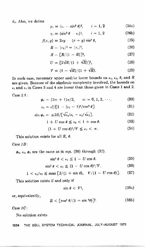
d2. Also, we definepi = (Ki - sin2 0)i, = 1, 2 (24a)
qi = (sin2 0 - Ki) i = 1, 2 (24b)
f(x, y) = 2xy - (x y) sin2 0, (25)
R= Irhi2 (26)
S = [R/(1 - (27)
U = [2-0-/(1 + (28)
V = (1 - -a)/(1 + (29)
In each case, necessary upper and/or lower bounds on K1, K2, 0, and Rare given. Because of the algebraic complexity involved, the bounds onKi and K2 in Cases 3 and 4 are looser than those given in Cases 1 and 2.
Case 1A:4)1 = (2m + 1)7/2, m = 0, 1, 2, (30)
K2 = K1/[1 - (Ki - 1)2/cost 0]. (31)
sin 4)2 = ±2S/[ 2/K1 - Ki/A1ic21 (32)
1 + U cos 0 Ki < 1 ± cos 0. (33)
(1 + U cos 0)2/V < K2 < OD . (34)
This solution exists for all R, 0.
Case 1B:
01, K2, 4)2 are the same as in eqs. (30) through (32).
sin2 0 < Ki < 1 -U cos 0. (35)
sin2 0 < K2 < (1 cos 0)2/V. (36)
1 < K1/K2 < max [2/(1 sin 0), V/(1 -U cos 0)]. (37)
This solution exists if and only if
sin 0 < Vi, (38a)
or, equivalently,R < [cos2 0/ (1 + sin 20)]2. (38b)
Case 1C:
No solution exists.
1034 THE BELL SYSTEM TECHNICAL JOURNAL, JULY -AUGUST 1975

Case 2A := (2ni 1)7r/2, »i = 0, 1, 2, . (39)
K2 = Ki. (40)
sin c62 = +28 cos 0p7p2. [(Ki - 1) sill 012. (41)
Ki > Ka ( >1), (42)
K2 > K (>1),
where K is the root larger than unity of the quartic equation
(43)
(W - 1)0 + 2(2 -W sine 0)0 - (6 + TV sin' 0 cos2 0)K2+ 2(2 + W sin4 0)K - (1 W sin' 0) =
where
0, (44)
W = [2S cos 0/sin2 012. (45)
This solution exists if and only if
sin 0 > U,
or, equivalently,R < [sin2 / (1 + cos2 0)12.
(46a)
(46b)
Case 2B:
01, K2, 42 are the same as in eqs. (39) through (41).
sin 0 < Ki Kb ( <1) ,
sing 0 < K 2 < Kp ( <1) ,
(47)
(48)
where Kb is the positive root less than unity of the quartic equation (44).This solution exists for all R, 0.
Case 2C:
On K2 are the same as ill eqs. (39) and (40).
sinh al = 2S cos 0piq2/[(1 - sin 012. (49)
sine 0 < Ki < sin 0. (50)
sin4 0 < K2 < sin2 0. (51)
This solution exists for all R, 0. It has been previously found byKard.8
Cases 3A, 3B:
No solutions exist.
MULTILAYER DIELECTRICS 1035

Case 8C :
cos (200 = f(Ki, 1) f(Ki, K2) /UK' - 1) (Ki - K2) sin4 0]. (52)
2-Ccig2f (Ki, 1)sinh a2 = (53)
Ki) - K2) sin2 0[Y - (K2 + X2) cos2
S = Aici(K2 - X) cos 0/[Y - (K2 + X2) cos2 014, (54)
whereX =- f(K1,102.)/[(1 + sin2 (55)
Y B K2(1 - K2) (Ki - 1)2/(1 + Kr). (56)
Ki > {1 + 3 cos2 0 + [8 cos2 0(1 + cos2 O) ]i /sin2 0. (57)
sin2 0 cos2 0/(1 + cos2 0) < K2 sin2 0/(1 + cos2 0). (58)
This solution exists if and only if
sin 0 > (2/S)4{ C(1 + 32/2782)1 111
- C(1 + 32/2782)1 - 1J414, (59a)
or, equivalently,R > 8 cos2 / (8 cos2 0 + sin' 0). (59b)
Cases 4A, 4B:
No solutions exist.
Case 4C:cosh 2cri = (1 + KO (K2 + K1)/[(l - (K2 - (60)
2 Artci K2(1 + Ki)qi.p2tan 02 = 4./
f-it (61)
J K2)[(1 -r K2) kKi 1- K2112
S = AYci(K2 - X)/[COS Oqi(K2 + X2)4],
where X is given in eq. (55).
Ki < sin2 0.
K2 > sin2 0.
This solution exists for all R, 0.
Discussion:
(62)
(63)
(64)
The above exhausts all possible solutions for a symmetric three -layerdielectric with no polarization dependence. The choice of the par-ticular solution to implement in a given problem depends on the desiredvalues of R and 0, the available dielectric materials, and whether
1036 THE BELL SYSTEM TECHNICAL JOURNAL, JULY-AUGUST 1975

having dielectric layers surrounded by air (Type A solution) or aprism realization (Type B or C solution) is more suitable.
Cases 1A and 2A, which are the only possible Type A solutions,require large values for the dielectric constants and/or the angle ofincidence to achieve moderate or large values of R. This point isillustrated for R = 0.5 in the design examples given in Section VIII.
In Case 2, the required relation between K1 and Kg given in eq. (40)has an advantage for the prism realizations in Cases 2B and 2C. Inthese two cases, since K2 < K1 < 1, eqs. (16) and (40) give 2 = 1,el = K1/K2, and Er = 1/K2 = e?. Thus, ei can also be used as a quarter -wave transformer to match the outer surfaces of the prisms.
As in the single -layer prism solution given in Section IV, one canvary R in Cases 1 and 2 without affecting the polarization independenceby simply changing d2. This is particularly convenient in the prismrealizations in Cases 1B, 2B, and 2C with 2 = 1 (air) since, in thiscase, d2 can be changed continuously. Case 2C is unique in that onecan obtain any value of R from zero to unity by varying d2 from zeroto infinity. In Cases 1A, 1B, 2A, and 2B, varying d2 results in a periodicvariation of R between zero and a maximum value less than unity.Varying d1 or d2 in Cases 3 or 4 results in a polarization -dependentoperation.
Cases 1A, 2B, 2C, and 4C have solutions for all R and 0. This is nottrue for the remaining three cases, 1B, 2A, and 3C, as indicated by eqs.(38), (46), and (59). However, one should note that the numericalvalues of et, el, and and not necessarily the limitations on R and 0,often determine whether or not any particular case can be used inpractice.
In Case 4C, eq. (46) indicates that one can have K2 = 1. In this case,given that K1 < 1 from eq. (63), eq. (16) gives 1 = 1 and et = e2= 1/Ki. Thus, the prism solution can be realized by using one dielectricmaterial with air separations. This is not true for any of the other cases.
VI. SYMMETRIC MULTILAYER SOLUTIONS
When there are more than three layers, an exhaustive analysissimilar to that given in the previous section becomes quite involved.However, two relatively simple classes of solutions for a symmetricmultilayer dielectric with no polarization dependence can be obtainedby generalizing Cases 1 and 2 of the symmetric three -layer dielectric.First, one should note that symmetry requires that the number oflayers n be odd, i.e.,
n = 2/ 1, = 1, 2, . (65)
MULTILAYER DIELECTRICS 1037
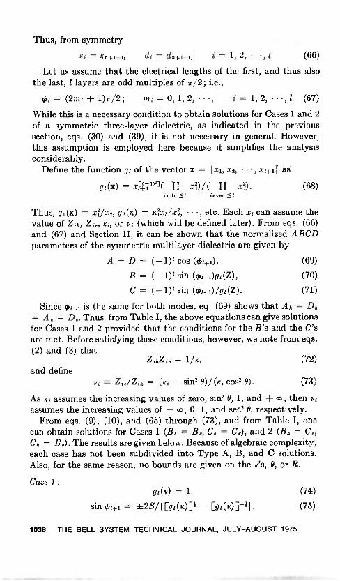
Thus, from symmetry
Ki = di = dn+1-i, = 1,2, , /. (66)
Let us assume that the electrical lengths of the first, and thus alsothe last, / layers are odd multiples of 7/2; i.e.,
= (2mi + 1)r/2; in 1 = 0, 1, 2, , i = 1, 2, , 1. (67)
While this is a necessary condition to obtain solutions for Cases 1 and 2of a symmetric three -layer dielectric, as indicated in the previoussection, eqs. (30) and (39), it is not necessary in general. However,this assumption is employed here because it simplifies the analysisconsiderably.
Define the function gi of the vector x = {xi, x2, , xi+1} as
g1(x) x47')11( IIiodd
A)/( fl xD.ieven"1
(68)
Thus, g1 (x) = x7/x2, g2(x) = x?x3/x3, , etc. Each xi can assume thevalue of Zih, Zie, Ki, or vi (which will be defined later). From eqs. (66)and (67) and Section II, it can be shown that the normalized ABCDparameters of the symmetric multilayer dielectric are given by
A = D = (-1)1 cos (86z+1), (69)
B = (-1)l sin (41÷1)g1(Z),
C = ( -1)1 sin (01+1)/gi(Z).
(70)
(71)
Since cki+i is the same for both modes, eq. (69) shows that A,, = Dh= A. = D.. Thus, from Table I, the above equations can give solutionsfor Cases 1 and 2 provided that the conditions for the B's and the C'sare met. Before satisfying these conditions, however, we note from eqs.(2) and (3) that
ZihZie = 1/Kiand define
(72)
ZielZih = (Ki sin' 0)/ (Ki cos2 0) (73)
As Ki assumes the increasing values of zero, sin2 0, 1, and + 00, then viassumes the increasing values of - 00, 0, 1, and sect 0, respectively.
From eqs. (9), (10), and (65) through (73), and from Table I, onecan obtain solutions for Cases 1 (Bh = Be, Ch = Ce), and 2 (B,, = C.,Ch = Be). The results are given below. Because of algebraic complexity,each case has not been subdivided into Type A, B, and C solutions.Also, for the same reason, no bounds are given on the K's, 0, or R.
Case 1:gi(v) = 1. (74)
sin rti+i = ±2S/1 [gi(sc)]i - [g1(x)]-41. (75)
1038 THE BELL SYSTEM TECHNICAL JOURNAL, JULY-AUGUST 1975
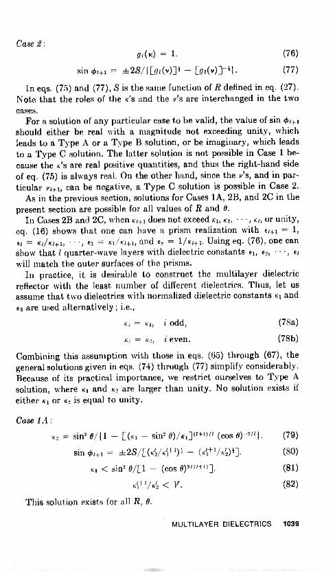
Case 2:g1(x) = 1.
sin chi -f-1 = ±28/1 Egi(v)il
(76)
(77)
In eqs. (75) and (77), S is the same function of R defined in eq. (27).Note that the roles of the K's and the V'S are interchanged in the twocases.
For a solution of any particular case to be valid, the value of sin 0/44should either be real with a magnitude not exceeding unity, whichleads to a Type A or a Type B solution, or be imaginary, which leadsto a Type C solution. The latter solution is not possible in Case 1 be-cause the K's are real positive quantities, and thus the right-hand sideof eq. (75) is always real. On the other hand, since the v's, and in par-ticular pi+i, can be negative, a Type C solution is possible in Case 2.
As in the previous section, solutions for Cases 1A, 2B, and 2C in thepresent section are possible for all values of R and O.
In Cases 2B and 2C, when /0_, does not exceed Ki, K2, , Kl, or unity,eq. (16) shows that one can have a prism realization with ei+i = 1,Et = Kdicti-i, , El = K1/K1+1, and ET = 1/Kt+1. Using eq. (76), one canshow that l quarter -wave layers with dielectric constants El, E2, , Er
will match the outer surfaces of the prisms.In practice, it is desirable to construct the multilayer dielectric
reflector with the least number of different dielectrics. Thus, let usassume that two dielectrics with normalized dielectric constants K1 andK2 are used alternatively ; i.e.,
Ki = Ki, i odd, (78a)
Ki = K2, (78b)i even.
Combining this assumption with those in eqs. (65) through (67), thegeneral solutions given in eqs. (74) through (77) simplify considerably.Because of its practical importance, we restrict ourselves to Type Asolution, where K1 and K2 are larger than unity. No solution exists ifeither K1 or K2 is equal to unity.
Case 1A:
K2 = sin' 0/11 - [(K1 - sin2 C)/KI]TH-nil (cos 0)-211). (79)
sin q5111 = ±2S/[(K2/K1+1)1 (Ki+Vic12)1]. (80)
K1 < sin2 0/[1 - (cos 9)21(1+1)]. (81)
< 1r. (82)
This solution exists for all R, O.
MULTILAYER DIELECTRICS 1039
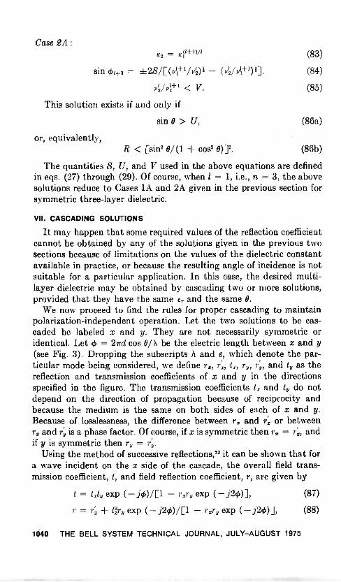
Case 2A:1+1)/1K2 = Ki( (83)
sin = ±2S/E(vii+Vv2)1 - (14/14+1)i]. (84)
vi,/pc+i < V. (85)
This solution exists if and only if
sin 0 > U,
or, equivalently,R < [sin2 0/ (1 + cos2 0)12.
(86a)
(86b)
The quantities S, U, and V used in the above equations are definedin eqs. (27) through (29). Of course, when 1 = 1, i.e., n = 3, the abovesolutions reduce to Cases 1A and 2A given in the previous section forsymmetric three -layer dielectric.
VII. CASCADING SOLUTIONS
It may happen that some required values of the reflection coefficientcannot be obtained by any of the solutions given in the previous twosections because of limitations on the values of the dielectric constantavailable in practice, or because the resulting angle of incidence is notsuitable for a particular application. In this case, the desired multi -layer dielectric may be obtained by cascading two or more solutions,provided that they have the same Er and the same 0.
We now proceed to find the rules for proper cascading to maintainpolarization -independent operation. Let the two solutions to be cas-caded be labeled x and y. They are not necessarily symmetric oridentical. Let cfi = 2rd cos 0/X be the electric length between x and y(see Fig. 3). Dropping the subscripts h and e, which denote the par-ticular mode being considered, we define r2, rzJ tz, ry, riv, and tu as thereflection and transmission coefficients of x and y in the directionsspecified in the figure. The transmission coefficients tz and ty do notdepend on the direction of propagation because of reciprocity andbecause the medium is the same on both sides of each of x and y.Because of losslessness, the difference between rz and r'x or betweenry and r; is a phase factor. Of course, if x is symmetric then rx = r', andif y is symmetric then ry =
Using the method of successive reflections," it can be shown that fora wave incident on the x side of the cascade, the overall field trans-mission coefficient, t, and field reflection coefficient, r, are given by
t = tzty exp ( -jcb)/[1 - rxry exp ( -./20)], (87)
r = exp ( - j20) /[1 - rxry exp ( -,j20)], (88)
1040 THE BELL SYSTEM TECHNICAL JOURNAL, JULY -AUGUST 1975

xd
Fig. 3-Cascading of two polarization -independent solutions x and y to obtain anoverall polarization -independent solution.
where we recall that a subscript of h or e has been dropped from all theis and r's.
Since x and y are polarization -independent solutions, then, from eq.(14) or Table I, rxhryh = ±rxerye. Only the positive sign is acceptable,otherwise the magnitude of the denominators in eqs. (87) and (88)would be different for the h- and e -modes, which will result in a polari-zation -dependent operation for the cascade. Thus, the sign of re/rhshould be the same for all the cascaded sections; i.e., one can only havea combination of Cases 1 and 3 or Cases 2 and 4.
Let the abbreviation i*j = k mean : "Cascading Cases i and j givesCase k." It can be shown from eqs. (87) and (88) and Table I that
1*1 = 3*3 = 1, 1*3 = 3*1 = 3, (89a)
2*2 = 4*4 = 2, 2*4 = 4*2 = 4. (89b)
Let the required overall power reflection coefficient of the cascade be
R = jr12, (90)
and let it be realized by two identical cascaded sections each having apower reflection coefficient R,. Then, one can write
= r Rtejoi, (91)
MULTILAYER DIELECTRICS 1041

where Oz is the phase angle of rz. This can be found given the e's, d's,and 0 by using eqs. (1) through (10). Substituting eq. (91) in eqs. (87)and (88), and defining
z - (92)
one obtainsR = + - R.)2/ (4R. sin2)1-1. (93)
Thus, for a given value of Rz, one can obtain any value of R satisfying
0 < R < 4Rx/(1 Rz)2. (94)
Note that the upper bound on R is larger than Rz. Conversely, for agiven value of R, one can use any value of Rz satisfying
[1 - (1 - R)1]2/R < Rz :5_ 1. (95)
The higher the value used for R1, the smaller is the overall bandwidth.
VIII. DIFFERENT INPUT AND OUTPUT MEDIA, AND ANTIREFLECTIONCOATINGS
Often, especially at optical wavelengths, the multilayer dielectric issupported by a substrate having a relative dielectric constant e, whichis, in general, different from that of the input medium, Er. In this case,general analysis of polarization -independent solutions is complicated.However, it can be shown that special solutions similar to those for thesymmetric (2/ 1) -layer dielectric given in Section VI can be easilyobtained. For this purpose, let 0, as before, be the angle of incidencein the Er medium. Assume that there are 1(..1) layers with relativedielectric constants ei, e2, El between the Er and E8 media. Thenormalized dielectric constants Ki, K2, , Ki are defined by eq. (1).In addition, we define
Es/cr. (96)
Further, as was done in Section VI, assume that each of the l layers iseffectively a quarter -wave thick at the given angle of incidence, i.e.,
= (2in 1)r/2; m = 0, 1, 2, , i= 1,2, , /. (97)
With the above definitions and assumptions, it can be shown fromeqs. (1) through (6) that the normalized input impedance as seen fromthe Er medium is given by
Zin = g1(Z), (98)
where Z = Z1, Z2, , Z1+11 and the function gi is defined in eq. (68).Thus, the reflection coefficient in the Er medium is given by
= (Zin - 1)/ (Zin + 1). (99)
1042 THE BELL SYSTEM TECHNICAL JOURNAL, JULY -AUGUST 1975
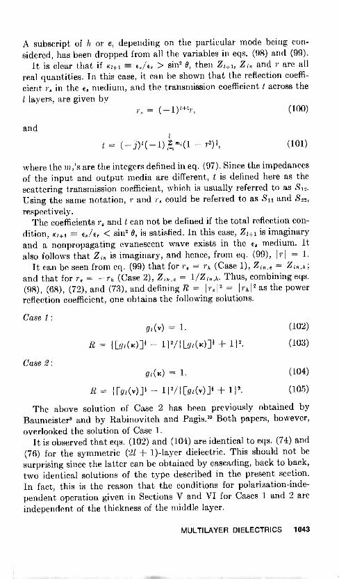
A subscript of 11 or e, depending on the particular mode being con-sidered, has been dropped from all the variables in eqs. (98) and (99).
It is clear that if Kr+i > sin2 0, then Z1+1, Zi and r are allreal quantities. In this case, it can be shown that the reflection coeffi-cient rs in the Es medium, and the transmission coefficient t across the1 layers, are given by
and
= (-1)1+'r, (100)
t = ( - ( -1) - r2)4, (101)
where the in i's are the integers defined in eq. (97). Since the impedancesof the input and output media are different, t is defined here as thescattering transmission coefficient, which is usually referred to as 812.Using the same notation, r and r could be referred to as 811 and 822,respectively.
The coefficients rs and I can not be defined if the total reflection con-dition, Kr+i = 8/ Er < sin' 0, is satisfied. In this case, Z/±1 is imaginaryand a nonpropagating evanescent wave exists in the e. medium. Italso follows that Z i is imaginary, and hence, from eq. (99), I rl = 1.
It can be seen from eq. (99) that for re = rh (Case 1), = Z in,h;
and that for re = - rh (Case 2), Zin, = 1/Zi,h. Thus, combining eqs.(98), (68), (72), and (73), and defining R = Irel2 = 1rh12 as the powerreflection coefficient, one obtains the following solutions.
Case 1:
Case 2:
gi(v) = 1.
R = - 112/ {Eill(K)11 + 112.
c/t(K)=1.
R = {Egi(v)li - 112/ {Egi(v)]i + 1)2.
(102)
(103)
(104)
(105)
The above solution of Case 2 has been previously obtained byBaumeister' and by Rabinovitch and Pagis.1° Both papers, however,overlooked the solution of Case 1.
It is observed that eqs. (102) and (104) are identical to eqs. (74) and(76) for the symmetric (2/ + 1) -layer dielectric. This should not besurprising since the latter can be obtained by cascading, back to back,two identical solutions of the type described in the present section.In fact, this is the reason that the conditions for polarization-inde-pendent operation given in Sections V and VI for Cases 1 and 2 areindependent of the thickness of the middle layer.
MULTILAYER DIELECTRICS 1043
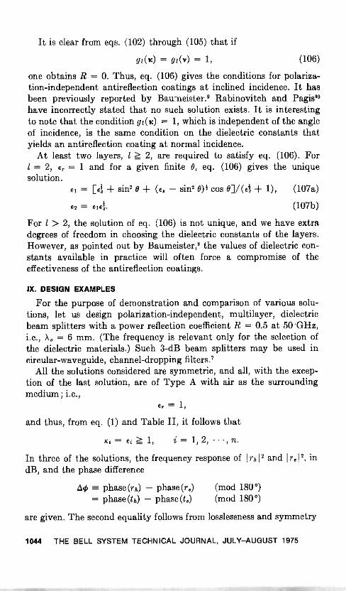
It is clear from eqs. (102) through (105) that if
g i(tc) = g z(v) = 1, (106)
one obtains R = 0. Thus, eq. (106) gives the conditions for polariza-tion -independent antireflection coatings at inclined incidence. It hasbeen previously reported by Bau-neister.' Rabinovitch and Pagisl°have incorrectly stated that no such solution exists. It is interestingto note that the condition gi(x) = 1, which is independent of the angleof incidence, is the same condition on the dielectric constants thatyields an antireflection coating at normal incidence.
At least two layers, 1 > 2, are required to satisfy eq. (106). For1 = 2, er = 1 and for a given finite 0, eq. (106) gives the uniquesolution.
el = [et ± sins 0 ± (es - sine 0)1 cos 0]/(ei + 1), (107a)
2 = 14. (107b)
For 1 > 2, the solution of eq. (106) is not unique, and we have extradegrees of freedom in choosing the dielectric constants of the layers.However, as pointed out by Baumeister,' the values of dielectric con-stants available in practice will often force a compromise of theeffectiveness of the antireflection coatings.
IX. DESIGN EXAMPLES
For the purpose of demonstration and comparison of various solu-tions, let us design polarization -independent, multilayer, dielectricbeam splitters with a power reflection coefficient R = 0.5 at 50 GHz,i.e., X0 = 6 mm. (The frequency is relevant only for the selection ofthe dielectric materials.) Such 3 -dB beam splitters may be used incircular-waveguide, channel -dropping filters.'
All the solutions considered are symmetric, and all, with the excep-tion of the last solution, are of Type A with air as the surroundingmedium; i.e.,
er =
and thus, from eq. (1) and Table II, it follows that
K{= ei 1, i= 1, 2, , n.
In three of the solutions, the frequency response of Irh12 and Ire! 2, indB, and the phase difference
phase (rh) - phase (re) (mod 180°)= phase(th) - phase (te) (mod 180°)
are given. The second equality follows from losslessness and symmetry
1044 THE BELL SYSTEM TECHNICAL JOURNAL, JULY-AUGUST 1975

Table Ill - Some low -loss dielectrics at millimeter wavelengths
Dielectric Dielectricconstant Loss tangent
Frequencyrange of
measurementsReference No.
KearfottHigh -Purity 9.4 0.00017 14 to 50 GHz 24Alumina
Polystyrene 2.54 0.0012 10 to 25 GHz 25
Teflon 2.1 0.0005 50 to 70 GHz Unpublishedreport
Eccofoam PS* 1.02 to 2.0 0.0004 10 GHz 26
* This is a CO2 foamed polystyrene whose density can be adjusted to yield anydielectric constant in the range specified. It is not clear how the Rayleigh scatteringby the CO2 bubbles will affect the loss tangent at frequencies higher than 10 GHz.
since, under these conditions, the difference between the phases of7. and t is ±90° at all frequencies as can be deduced from eqs. (8)through (10).
The dielectric materials employed in our solutions will be chosenfrom those given in Table III. Because of their low loss, these materialsare suitable for use at millimeter wavelengths. Other suitable dielec-trics can be found in Refs. 24 and 25.
9.1 Symmetric three -layer, Case 1A solution (El, E2, ei)
With R = 0.5, eqs. (33) and (34) require that 1.64 ei < 1.71 ande2> 15.74 for 6 = 45'; 1.46 el < 1.5 and e2>_12.34 for 0 = 60°;or 1.23 ei < 1.26 and 2 > 8.90 for 0 = 75°. It is difficult to realizea solution at millimeter wavelengths for 0 less than about 60° becauseof the high required value e2. However, for 0 75°, the value of E2 canbe realized by Kearfott Alumina ( = 9.4). The corresponding lowvalue of el can be obtained by using Eccofoam PS, or foamed rubbersuch as Buna S Rubber whose dielectric constant can be extrapolatedto be 1.26 at 50 GHz.25 Thus, with el = 1.26 and e2 = 9.4, eq. (31)gives 0 = 73.43°, eqs. (4a) and (30) give di/X. = 0.428 ± m 1 X 0.856,and eqs. (4a) and (31) give d2/Xo = 0.078 + m2 X 0.172, where miand m2 are integers.
The frequency response of this solution is given in Fig. 4 for m1 = 111 2= 0. The large required value of 0 makes this solution undesirable.
9.2 Symmetric three -layer, Case 2A solution (El, E2,
With R = 0.5, eq. (46) requires that 0 > 65.53°; and eqs. (40) and(42) through (44) require that el > 4.61 and e2 = el > 21.23 for0 = 70° ; el > 2.09 and e2 = > 4.38 for 6 = 75° ; and el > 1.58
MULTILAYER DIELECTRICS 1045

-2.0
-2.5
0cs7 -3.0
00
-3.5
-4.0
I I I 1 \_-
I
\,\
I
\
I I I 1 I 1 1 1 1 1
_--
_ -1rh12
---
\ ,\.
- --- - - -----
, ..---,\
\:- ..4C- Ire12 -...--""\ -
Akp \- -- \ -
1 I 1 1 1 1 1 1 1 1 I 1 \ 1 1 1 1
0.9 0.95 1 0
NORMALIZED FREQUENCY fifo
1.05
10
5
0
5
-101.1
Fig. 4-Frequency response of the solution in 9.1 [three -layer, Type 1A solutionwith 0= 73.43°, el =1.26 (Buna S Rubber), 2 = 9.4 (Kearfott Alumina), d,/X0 = 0.428,and d2/X, = 0.078].
and E2 = e? > 2.49 for 0 = 78°. In the last case, the solution can berealized by Eccofoam PS (E = 1.59) and polystyrene (E = 2.54). Justas in the solution in Section 9.1, the required large value of 0 makes thissolution undesirable. For symmetric multilayer, Type -2A solutions withmore than three layers of two dielectrics, eq. (86) shows that 0 is stillrequired to exceed 65.53°.
9.3 Symmetric five -layer, Case 1A solution Ea, El, El)
For R = 0.5 and 1 = 2, i.e., n = five layers, eqs. (79), (80), and (81)can be satisfied with ei = e3 = 2.1 (Teflon), E2 = 9.4 (KearfottAlumina), and 0 = 46.91°, which is a convenient angle of incidence.Further, eqs. (4a) and (67) give di/X0 = 0.200 + m1 X 0.399 andd2/X = 0.084 + m2 X 0.168, and eqs. (4a) and (80) give d3/Xo
= 0.103 + 1113 X 0.399, where m 1, m2, and m3 are integers. The fre-quency response of this solution is given in Fig. 5 for mi = 1112 =17 1 3 = 0.
9.4 Symmetric seven -layer, Case 1A solution Es, et, Ejy 2, El)
For R = 0.5 and 1 = 3, i.e., n = seven layers, eqs. (79), (80), and(81) can be satisfied with el = e3 = 2.54 (polystyrene), E2 = E4 = 9.4(Kearfott Alumina), and 0 = 47.52°. Further, eqs. (4a) and (67) givedi/X = d3/X0 = 0.177 + in' X 0.354 and d2/X = 0.084 + n2,2 X 0.168,
1046 THE BELL SYSTEM TECHNICAL JOURNAL, JULY-AUGUST 1975

and eqs. (4a) and (80) give d4/X0 = 0.026 + 1114 X 0.168, where m 1,m2, and ma are integers. This solution has a narrower bandwidth thanthe solution in 9.3.
9.5 Symmetric seven -layer, Case 1A solution obtained by cascading twoidentical, symmetric three -layer, Case 1A solutions
E2, El, 1.0, el, E2, ei)
With R = 0.5, eq. (95) shows that Rz, the power reflection coeffi-cient of each cascaded three -layer section, should not be less than0.1716; thus let us choose Rz = 0.1716. In this case, eqs. (31), (33),and (34) can be satisfied with el = 1.6 (Eccofoam PS), e2 = 9.4(Kearfott Alumina), and 0 = 45.30°. Further, eqs. (4a) and (30) gived1/X0 = 0.239 + ml X 0.478 and eqs. (4a) and (32) give d2/X. = 0.038+ m2 X 0.168.
To find the width d of the air separation, one should first find thephase (1)= of the reflection coefficient of each cascaded three -layersection. By substituting the values of ei, 2, d1, d2, and 0 obtained abovein eqs. (2) through (10), one finds that os = 43.59°. With R = 0.5and Rz = 0.1716, eq. (93) gives = ±90° (mod 180°), and hence,the electrical length of the air spacing between the two three -layersections is found from eq. (92) to be it, = 133.59° + m X 180°, wherein is an integer. Thus, from eq. (4a) with er = Ki = 1, d/ A = 0.528
-2.0
-2.5
U,-1wCO
,U
wO
3.0
0-J0
-3.5
-4.0
1
-
2--.
1 1
........
1
-....,,
I 1 1 1 1 1 1 1 1 1 1 I
_
-.... .....
......".,-- - -
.....*"........*".."
........ ....-''
_- ##
..,.... ..,,..e
..,#'4F-.. - Irel2
.......,
Aso
N --
---####- #4
1
#
1 1
.."#.e
1 I I 1 I I 1
N
1 1
NN
1 1
---
N -IN I
0 9 0.95 1.0
NORMALIZED FREQUENCY f/f01.05
10
5
0
-5
-101.1
Fig. 5-Frequency response of the solution in 9.3 [five -layer, Type lA solution with0 = 46.91°, ei =. 3 = 2.1 (Teflon), E2 = 9.4 (Kearfott Alumina), diA0 = 0.200,d2/X = 0.084, and da/Xo = 0.103].
MULTILAYER DIELECTRICS 1047

-2.
-2.5
-3.0
-3.5
-4.0
1 I I I.-
,..
IIII III1
I i I I ..1
....
.-_ ir,12
...,,,......"
-,
___--------...- - --V-... N Irel2
-
.........--__
....... .0..,25.---
we
_,
....,
-
-.--
1 1 11 1 1 1
1
1111 1 1 I
-,--
1
0.9 0.95 1 0
NORMALIZED FREQUENCY f/fo
Fig. 6-Frequency response of the solution in 9.6 [three -layer, Type 2C prism solu-tion with 0=45°, Er =2.54 (polystyrene), ei =1.59 (Eccofoam PS), e2=1, di/X2= 0.439,and d2/X. = 0.236].
10
5
-101.05 11
m X 0.711. This solution has a narrower bandwidth than the solu-tion in 9.3.
9.6 Symmetric three -layer, Case 2C prism solution (er, El, 1.0, E1, Er)
Choosing 0 = 45° and E2 = 1.0, eqs. (16), (40), (50) and (51) give1.414 < el < 2 and 2 < Er = e < 4. Thus, the solution can be ob-tained with el = 1.59 (Eccofoam PS) and Er = e? = 2.54 (polysty-rene). Further, eqs. (4a) and (39) give di/X0 = 0.439 + m X 0.879,where in is an integer, and with R = 0.5, eqs. (4a), (4b), and (49)give d2/A0 = 0.236. The frequency response of this solution is givenin Fig. 6. for in = 0 and under the assumption that the outer surfacesof the prisms are perfectly matched. As mentioned at the end of Sec-tion V, the matching can be accomplished by using a quarter -wavelayer having a dielectric constant el = 1.59 (Eccofoam PS).
X. ACKNOWLEDGMENT
The author wishes to thank J. A. Arnaud for useful suggestions.
REFERENCES
1. M. Born and E. Wolf, Principles of Optics, Oxford : Pergamon Press, 1965.2. A. F. Harvey, "Optical Techniques at Microwave Frequencies," Proc. IEE,
B106 (March 1939), pp. 141-157.3. It. Trembley and A. Boivin, "Concepts and Techniques of Microwave Optics,"
Applied Optics, 5, No. 2 (February 1966), pp. 249-278.4. It. Levy, "Directional Couplers," in Advances in Microwaves, 1, L. Young, Ed.,
New York : Academic Press, 1966, pp. 196-205.
1048 THE BELL SYSTEM TECHNICAL JOURNAL, JULY -AUGUST 1975

5. J. J. Taub, H. J. Hindin, 0. F. Hinckelmann, and M. L. Wright, "SubmillimeterComponents Using Oversized Quasi -Optical Waveguide," IEEE Trans.Microwave Theory Tech., MTT-11, No. 5 (September 1963), pp. 338-350.
6. M. Koyama and S. Shimada, "The Quasi -Optical Filters Used for the DomesticSatellite Communication System," Electr. and Commun. in Japan, 56-B,No. 3 (March 1973), pp. 74-81.
7. E. A. J. Marcatili and D. L. Disbee, "Band -Splitting Filter," B.S.T.J., 40,No. 1 (January 1961), pp. 197-212.
8. P. G. Kard, "On the Elimination of the Doublet Structure of the TransmissionBand in a Total -Reflection Light Filter," Optics and Spectroscopy, (Transla-tion of Optika i Spektroskopiia), VI, No. 3 (March 1959), pp. 244-246.
9. P. Baumeister, "The Transmission and Degree of Polarization of Quarter -WaveStacks at Non -Normal Incidence," Optica Acta, 8, No. 2 (April, 1961), pp.105-119.
10. K. Rabinovitch and A. Pagis, "Polarization Effects in Multilayer DielectricThin Films," Optica Acta, 21, No. 12 (December 1974), pp. 963-980.
11. R. B. Adler, L. J. Chu, and R. M. Fano, Electromagnetic Energy Transmission andRadiation, New York: John Wiley, 1965, pp. 354-362.
12. J. R. Wait, Electromagnetic Waves in Stratified Media, New York : PergamonPress, 1962, pp. 10-15.
13. P. Leurgans and A. F. Turner, "Frustrated Total Reflection Interference Filters,"J. Opt. Soc. Am., 37, No. 12 (December 1947), p. 983.
14. M. Born and E. Wolf, Ref. 1, pp. 350-351.15. H. D. Raker and G. R. Valenzuela, "A Double -Prism Attenuator for Millimeter
Waves," IRE Trans. Microwave Theory Tech., (Correspondence), MTT-10,No. 5 (September 1962), pp. 392-393.
16. H. J. Hindin and J. J. Taub, "Oversized Waveguide Directional Coupler," IRETrans. Microwave Theory Tech. (Correspondence), MTT-10, No. 5 (Septem-ber 1962), pp. 394-395.
17. T. Makimoto and T. Sueta, "Prism Directional Couplers Making Use of BrewsterAngle Transmission," Memoirs of the Institute of Scientific and Industral Re-search, Osaka University, Japan, 21, 1964.
18. T. Sueta, N. Kumagai, and S. Kurazono, "Wideband Quasi -Optical Prism Com-ponents," Elect. and Commun. in Japan, 49, No. 3 (March 1966), pp. 100-106.
19. R. G. Fellers and J. Taylor, "Internal Reflections in Dielectric Prisms," IEEETrans. Microwave Theory Tech., MTT-12, No. 6 (November 1964), pp.584-587.
20. R. E. Collin and J. Brown, "The Design of Quarter -Wave Matching Layers forDielectric Surfaces," Proc. IEE, 103C (September 1955), pp. 153-158.
21. T. Morita and S. B. Cohn, "Microwave Lens Matching by Simulated Quarter -Wave Transformers," IRE Trans. Antennas and Propagation, AP -4, No. 1(January 1965), pp. 33-39.
22. E. M. T. Jones and S. B. Cohn, "Surface Matching of Dielectric Lenses,"J. of Appl. Phys., 26, No. 4 (April 1955), pp. 452-457.
23. M. Born and E. Wolf, Ref. 1, pp. 323-329.24. Lab. for Insulation Research, M.I.T., Tables of Dielectric Materials, 5, April
1957.25. A. R. Von Hipple, ed., Dielectric Materials and Applications, M.I.T. Press and
John Wiley, New York, 1954.26. Emerson and Cuming, Inc., Dielectric Materials Division, "Eccofoam PS-
Low-Loss Adjustable Dielectric Constant Foam," Technical Bulletin No.6-24, Canton, Massachusetts, June 15,1970.
MULTILAYER DIELECTRICS 1049

-r

Copyright © 1975 American Telephone and Telegraph CompanyTHE BELL SYSTEM TECHNICAL JOURNAL
Vol. 54, No. 6, July -August 1975Printed in 17.5..4.
A Method for Calculating Rain AttenuationDistributions on Microwave Paths
By S. H. LIN
(Manuscript received January 9, 1975)
An engineering method is proposed for calculating rain attenuationdistributions for frequencies greater than 10 GHz and for paths of arbitrarylength. The technique is based upon the observed approximate lognormalityof rain attenuation and rain rate statistics within the range of interest;it reflects local meteorology through incorporation of the observed pointrain rate distribution. Some important parameters in the resulting formulasare determined empirically from experimental data. Sample calculatedresults agree well with available experimental data from. Georgia, NewJersey, and Massachusetts. This new technique may prove useful forengineering radio paths at frequencies above 10 GHz. Sample calculationsof expected outage probability are given for 11- and 18-GHz radio linksat Atlanta., Georgia, as a function of repeater spacing and transmissionpolarization .
I. INTRODUCTION
An important problem in designing radio relay systems at fre-quencies above 10 GHz is the radio outage caused by rain attenuation.Determination of the appropriate radio repeater spacings for economicand reliable operation requires a knowledge of the probability dis-tribution of rain attenuation as a function of repeater spacing atvarious geographic locations. Most available data on rain rate sta-tistics are measured by a single rain gauge at a given geographic loca-tion. A procedure for calculating a rain attenuation distribution froma point rain rate distribution is, therefore, needed.
The results of rain gauge network measurements'-' indicate, how-ever, that the measured short-term distributions of point rain ratevary significantly from gauge to gauge. For example, at Holmdel,New Jersey, there was considerable variation' among the measuredpoint rain rate distributions obtained from 96 rain gauges located ina grid with 1.3 -km spacing over a 6 -month period. Among these 96distributions, the incidence of 100-mm/h rains is higher by a factor of
1051
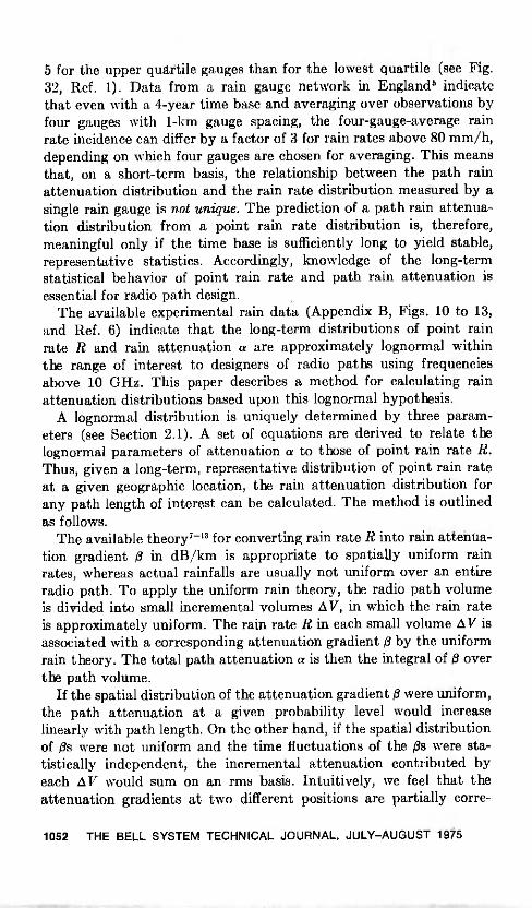
5 for the upper quartile gauges than for the lowest quartile (see Fig.32, Ref. 1). Data from a rain gauge network in England' indicatethat even with a 4 -year time base and averaging over observations byfour gauges with 1 -km gauge spacing, the four -gauge -average rainrate incidence can differ by a factor of 3 for rain rates above 80 mm/h,depending on which four gauges are chosen for averaging. This meansthat, on a short-term basis, the relationship between the path rainattenuation distribution and the rain rate distribution measured by asingle rain gauge is not unique. The prediction of a path rain attenua-tion distribution from a point rain rate distribution is, therefore,meaningful only if the time base is sufficiently long to yield stable,representative statistics. Accordingly, knowledge of the long-termstatistical behavior of point rain rate and path rain attenuation isessential for radio path design.
The available experimental rain data (Appendix B, Figs. 10 to 13,and Ref. 6) indicate that the long-term distributions of point rainrate R and rain attenuation a are approximately lognormal withinthe range of interest to designers of radio paths using frequenciesabove 10 GHz. This paper describes a method for calculating rainattenuation distributions based upon this lognormal hypothesis.
A lognormal distribution is uniquely determined by three param-eters (see Section 2.1). A set of equations are derived to relate thelognormal parameters of attenuation a to those of point rain rate R.Thus, given a long-term, representative distribution of point rain rateat a given geographic location, the rain attenuation distribution forany path length of interest can be calculated. The method is outlinedas follows.
The available theory7-" for converting rain rate R into rain attenua-tion gradient (3 in dB/km is appropriate to spatially uniform rainrates, whereas actual rainfalls are usually not uniform over an entireradio path. To apply the uniform rain theory, the radio path volumeis divided into small incremental volumes A V, in which the rain rateis approximately uniform. The rain rate R in each small volume A V isassociated with a corresponding attenuation gradient fl by the uniformrain theory. The total path attenuation a is then the integral of 13 overthe path volume.
If the spatial distribution of the attenuation gradient Q were uniform,the path attenuation at a given probability level would increaselinearly with path length. On the other hand, if the spatial distributionof fls were not uniform and the time fluctuations of the fls were sta-tistically independent, the incremental attenuation contributed byeach A V would sum on an rms basis. Intuitively, we feel that theattenuation gradients at two different positions are partially corre-
1052 THE BELL SYSTEM TECHNICAL JOURNAL, JULY-AUGUST 1975
lated, with a correlation coefficient that is a decreasing function ofthe spacing between the two positions. This behavior is described byintroducing a spatial correlation function for 13. This spatial correlationfunction is used in the calculation of lognormal parameters of pathattenuation a from those of attenuation gradient 13.
In this formulation, the appropriate incremental sampling volumeA V is of the order of 1 m3 and the corresponding appropriate raingauge integration time about 2 s, requiring, therefore, 2-s point rainrate distributions (see Section 2.3).
Tables II and III and Figs. 5 to 8, discussed in Section IV, presentcomparisons of calculated and measured attenuation distributions.The satisfactory correspondence appears to validate the method ofcalculation. Section V and Fig. 9 present the calculated results for theoutage probabilities of 11- and 18-GHz radio links in Georgia. SectionVI discusses some qualifications to the methodology.
Supporting material and mathematical derivations are given inAppendices A to D. Appendix E lists symbols and their definitions.
II. BASIC DEFINITIONS AND FORMULATION
2.1 Lognormal distributions of attenuation and rain rate
The equations approximating the rain attenuation distribution andpoint rain rate distribution are :
and
In A - In an,P[a(L) A] Po(L) lerfcV2Sa
(1)
In r - In R,P(R r) P0(0) erfc [ , (2)
where erfc denotes the complementary error function, Indenotes natural logarithm, S and SR are the standard deviations ofIn a and In R, respectively, during the raining time, an, and R, are themedian values of a and R, respectively, during the raining time, Po(L)is the probability that rain will fall on the radio path of length L, andPo(0) is the probability that rain will fall at the point where the rainrate R is measured. The definition and the determination of rainingtime, and hence Po(L) and Po(0), are discussed in Section 2.5. Themeasured distribution of point rain rate is a function of rain gaugeintegration time T.14-20 The appropriate integration time is about 2 sin our formulation as discussed in Section 2.3.
2.2 Radio path definition
C. L. Ruthroffn has defined a "radio path," giving a physical aswell as mathematical representation in the spatial volume significant
RAIN ATTENUATION 1053

to propagation considerations (Fig. 1). In essence, the "radio path"corresponds to the first Fresnel zone, a prolate ellipsoid of revolutionterminated at the ends by the transmitting and receiving antennas.
Since the first Fresnel zone is circularly symmetric with respect tothe path axis connecting the transmitting and receiving antennas, weadopt a cylindrical coordinate system (Fig. 1) coaxial with the path axis(z-axis) in the formulation.
The radius h(z) and the circular cross section Q (z) (see Fig. 1) of theradio beam at a distance z from the transmitter are
X z(L - z)r
and
(3)
Q (z) = irh2 (z), (4)
where X is the radio wavelength and L is the distance between trans-mitter and receiver. For example, at 18 GHz on a 5 -km path, theaverage beam radius, the average beam cross section, and the radiopath volume are about 3 m, 30 m2, and 150,000 m3, respectively.
2.3 Path integral formulation for rain attenuation
The spatial distribution of actual rainfall is usually nonuniform.The rain density, the point rain rate R, and the corresponding (point)rain attenuation gradient 13 are all functions of position (p, z) and oftime (t). The total rain attenuation a in dB incurred on a radio path oflength L (Fig. 1) is calculated by integrating the incremental attenua-tion da along the path
L L
a(t) = jo dz = J #,(z, Odz (5)
Q(Z) -0
L 1 i2i- h(z)13(p, 4), z, t) pdpd4)dz, (6)
f0 0
where1 f2r rh(z)
s 9(z, = Q(z) jo_o S(P, 4), z, pdpd4 (7)
is the average value of 0(p, 4, z, I) over the radio beam cross sectionQ (z) at a distance z from the transmitter, and
da (z, t) = 139(z, t)dz (8)
is the incremental attenuation experienced in the incremental segmentdz at a distance z from the transmitter.
To shorten the notations in the following equations, we use thevector s to denote the position (p, z) and dv to denote pdpd4)dz in thevolume integration.
1054 THE BELL SYSTEM TECHNICAL JOURNAL, JULY-AUGUST 1975
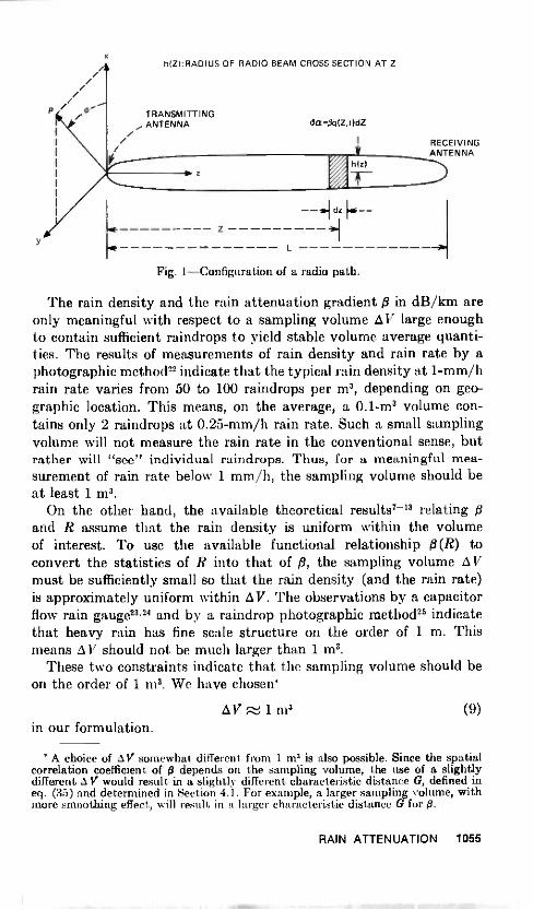
1,(Z):RADIUS OF RADIO BEAM CROSS SECTION AT Z
TRANSMITTINGANTENNA da=13q(Z,t)dZ
RECEIVINGANTENNA
L
dz
Fig. 1-Configuration of a radio path.
The rain density and the rain attenuation gradient in dB/km areonly meaningful with respect to a sampling volume AV large enoughto contain sufficient raindrops to yield stable volume average quanti-ties. The results of measurements of rain density and rain rate by aphotographic method22 indicate that the typical rain density at 1-mm/hrain rate varies from 50 to 100 raindrops per m3, depending on geo-graphic location. This means, on the average, a 0.1-m3 volume con-tains only 2 raindrops at 0.25-mm/h rain rate. Such a small samplingvolume will not measure the rain rate in the conventional sense, butrather will "see" individual raindrops. Thus, for a meaningful mea-surement of rain rate below 1 mm/h, the sampling volume should beat least 1 m3.
On the other hand, the available theoretical results' -13 relating 0and R assume that the rain density is uniform within the volumeof interest. To use the available functional relationship (R) toconvert the statistics of R into that of 13, the sampling volume A Vmust be sufficiently small so that the rain density (and the rain rate)is approximately uniform within AV. The observations by a capacitorflow rain gaugen," and by a raindrop photographic method" indicatethat heavy rain has fine scale structure on the order of 1 m. Thismeans A V should not be much larger than 1 m3.
These two constraints indicate that the sampling volume should beon the order of 1 m3. We have chosen*
A V ;,..1 1 m3 (9)in our formulation.
* A choice of AV somewhat different from 1 m3 is also possible. Since the spatialcorrelation coefficient of # depends on the sampling volume, the use of a slightlydifferent AV would result in a slightly different characteristic distance G, defined ineq. (35) and determined in Section 4.1. For example, a larger sampling volume, withmore smoothing effect, will result in a larger characteristic distance G for 13.
RAIN ATTENUATION 1055

Therefore, in this paper, 3(s, t) is defined as the rain attenuationgradient at time t, owing to rain in a 1-m3 sampling volume, A V,centered at s, and 13,(z, t) is the average value of 0(s, t) over the pathcross section Q (z) .
If A,, is the area of the collecting aperture of a rain gauge and VR
the average descent velocity of rainfall, then the appropriate raingauge integration time TAY to measure rain rate in a 1-m3 samplingvolume A V is
AVTAV (10)
A, V R
For example, if Au = 0.073 m2 (i.e., 12 -in. diameter), then TAT, isabout 2 s, assuming V R 7 m/s. In the measurements of raindrop sizedistributions, Laws and Parsons" have also used an integration timein the order of seconds during heavy rain. The Laws -and -Parsons rain-drop size distribution is the basis of most uniform rain theories forconverting R into 3. We therefore define R(s, t) as the point rain ratemeasured by a rain gauge with integration time T°V, located at s. Theshape of the 1-m3 sampling volume defined by the rain gauge is cy-lindrical and is considerably different from that of the incrementalAV. We assume that the long-term distributions of rain rates for thesetwo different shapes of 1-m' sampling volume are approximately thesame.
Based upon these definitions, we postulate that the long-term prob-ability distribution of R(s, 1) can be converted into the long-termprobability distribution of # (s, t) by a relationship discussed in thenext section.
The integration times of most available point rain rate data arelonger than the TAV s) required by this formulation. The depen-dence of point rain rate distribution on the rain gauge integration timein the range
1.5 s T 120 s (11)
has been determined by Bodtmann and Ruthroff" for a 2 -year (1971-1972) measurement at Holmdel, New Jersey. By using this experi-mental result and interpolation, we convert the available point rainrate distribution with T in the range (11) into a 2-s point rain ratedistribution.'
2.4 Average relationship between rain rate and rain attenuation gradient
The instantaneous relationship obtaining between the point rainrate R(s, 1) and the corresponding rain attenuation gradient gs, t)
This relationship has not yet been demonstrated lo be geographically independent.
1056 THE BELL SYSTEM TECHNICAL JOURNAL, JULY-AUGUST 1975

100
E 10
cc
UJ
zCC
CC
1
0.1
CALCULATED FOR V-POLARIZATION
0 CALCULATED FOR H-POLARIZATION
-- APPROXIMATION BY Q = -y Rn
I
FROM REF.7
I I I I I I
10-3 10-2 10-1 1
RAIN ATTENUATION GRADIENT 0 IN dB/Km10 40
Fig. 2-Theoretical relationship between rain rate and rain attenuation gradient.
depends the particular distribution of raindroporientations, the speed and local direction of the wind, and the raintemperature. The average relationship, assuming uniform rain density,spherical raindrops, and Laws -and -Parsons drop -size distribution, hasbeen calculated by Ryde and Ryde,"-" Medhurst,9 and Setzer."Recently, Morrison, Cross, and Chu,7.27 and Oguchi8 have refinedthese calculations by including the effects of nonspherical raindrops.Figure 2 shows this theoretical relationship* for transmission frequen-cies of 11, 18, and 30 GHz.
Many authors have pointed out that this average relationship be-tween the rain rate R and rain attenuation gradient p can be approxi-mately described by
= 7(X) Rn(x), (12)
where -y(X) and n (X) depend upon the radio wavelength X and thepolarization of the radio signal. Table I lists the estimated .y (X) andn (X) for 11, 18, 30, and 60 GHz.
In Fig. 2, the average of the absolute value of raindrop canting angle is assumed tobe 25 degrees. This angle has been found representative by Chu (Refs. 28 and 29) incomparisons of calculated results with experimental observations (Refs. 30 and 31) ofthe differential rain attenuation experienced by horizontally and vertically polarizedsignals on the same radio path.
RAIN ATTENUATION 1057

Table I - Parameters relating rain rate R and rain attenuationgradient /3
= -y Fin /3 in dB/km R in mm/hour
Frequency(GHz)
V-Pol H-Pol V-Pol H-Pol
11 0.013 0.015 1.22 1.2318.1 0.05 0.054 1.11 1.1430 0.15 0.17 1.04 1.0460* 0.7* 0.7* 0.814* 0.814*
* The 60-GHz parameters are estimated from results in Ref. 10 in which onlyspherical raindrops are considered.
Taking logarithms of both sides of eq. (12) yields
lnQ = ln ± n In R. (13)
From this equation, if the distribution of point rain rate R is approxi-mately lognormal in the range of interest, then the distribution ofattenuation gradient (3 will also be approximately lognormal (seeAppendix B). The distribution of 0 can therefore be written as:
[(14)
In B - InP($ B) Po(0) lerfc 1/2 Ss '
where 0n, is the median value of (3 during the raining time and So isthe standard deviation of In 0 during the raining time. Furthermore,eqs. (12) and (13) imply the relationships
So = 71 SR
and
(15)
ke. = 7' Ms. (16)
Equations (15) and (16) allow us to convert the lognormal distribu-tion (2) of R into the lognormal distribution (14) of 13, and vice versa.
2.5 Rainfall probability Po(0) and raining time
In principle, the probability of raining, Po (0), is obtained as the limit
lim P(R ----E P0(0). (17)E
An instant t is considered to be raining time if the condition
lim R(t) > e (18)
is satisfied. The lower cutoff threshold in most presently available rain
1058 THE BELL SYSTEM TECHNICAL JOURNAL, JULY-AUGUST 1975

7
6
5
4
3
2
RAIN GAUGE NETWORK DATA OFFLORIDA THUNDERSTORM PROJECT(REF.20)
EMPIRICAL CURVE DESCRIBEDBY EQ. (20)
ORLANDO,FLORIDA2 -MINUTE INTEGRATION TIME
0 5 10
PATH LENGTH L IN KM15 20
Fig. 3-Rain-gauge network data on path length dependence of rainfall proba-bility P0(L).
rate data is about 0.25 mm/h. Therefore, in practice, we approximate0+ in definitions (17) and (18) by 0.25 mm/h. The rationale for thisapproximation is twofold.
(i) Rain rates below 0.25 mm/h have practically no significanteffects on radio communication links at frequencies below 60GHz.
(ii) Rain rates below 0.25 mm/h cannot be measured accuratelyby most existing rain gauges with standard recording stripcharts.
At the present time, the probability P (R > 0.25 mm/h I T = 1 min)is available at only a few locations.14,18,20 For most locations, we canobtain P (R > 0.25 mm/h) with 1-h integration time from the WeatherBureau hourly precipitation data." The experimental results on theeffect of rain gauge integration time T on P0(0) in Florida's'," and
Japan" indicate that
P (R > 0.25 mm/h J T < 1 min)0.5 P (R >= 0.25 mm/h I T = 1 h). (19)
Therefore, we use Weather Bureau data and approximation (19) toestimate Po (0) at several locations of interest where direct measure-ment of Po (0) with 1 -min integration is not available.
RAIN ATTENUATION 1059
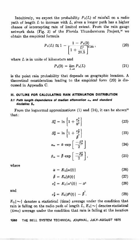
Intuitively, we expect the probability Po(L) of rainfall on a radiopath of length L to increase with L, since a longer path has a higherchance of intercepting rain of limited extent. From the rain gaugenetwork data (Fig. 3) of the Florida Thunderstorm Project," weobtain the empirical formula
1Po(L) 1
- Po(0)L2 0.014 ,
1 ±21.5
where L is in units of kilometers and
P0(0) = lim Po(L)
(20)
(21)
is the point rain probability that depends on geographic location. Atheoretical consideration leading to the empirical form (20) is dis-cussed in Appendix C.
III. OUTLINE FOR CALCULATING RAIN ATTENUATION DISTRIBUTION
3.1 Path length dependence of median attenuation am and standarddeviation S.
From the lognormal approximations (1) and (14), it can be shown"that:
where
and
4 = In {1 +Q2(22)SA = In { 1 + -12 (23)
2
am = c,exp [ (24)
= flexp [ (25)
a = EL{O) } (26)
= Eolgt) (27)
Qa = EL W(0 - a2 (28)
2
gti = E 0{ X32 (t)} # (29)
EL{,-} denotes a statistical (time) average under the condition thatrain is falling on the radio path of length L, E01,--,1 denotes statistical(time) average under the condition that rain is falling at the location
1060 THE BELL SYSTEM TECHNICAL JOURNAL, JULY-AUGUST 1975
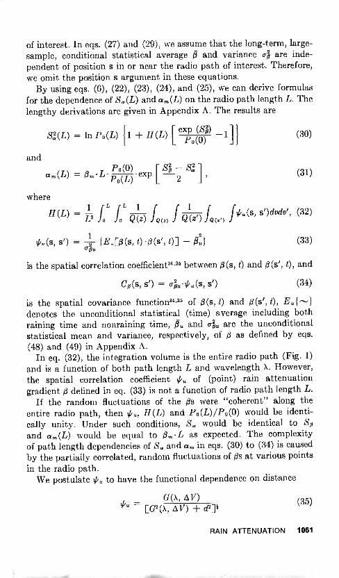
of interest. In eqs. (27) and (29), we assume that the long-term, large -sample, conditional statistical average ti and variance 0-A are inde-pendent of position s in or near the radio path of interest. Therefore,we omit the position s argument in these equations.
By using eqs. (6), (22), (23), (24), and (25), we can derive formulasfor the dependence of Sa (L) and am(L) on the radio path length L. Thelengthy derivations are given in Appendix A. The results are
and
SRL) = In Po(L) {1 H (L) [ exA((0S? 1 (30)
P.(0) is _«,,,(L) = L P 0(L) exP [
s2
Sa
where
(31)
1 fL rL1 1 1H (L)L2 ,l
s')dvdvi , (32)-2 ja Jo Q(z) ..1(2(z) J Q(z') 1(e) J
_
lku(s3 s') =1
{E.D(S, t) (s' - O2}0-13u
(33)
is the spatial correlation coefficient"," between 0(s, t) and 0(s', t), and
Co(s, s') = o-,26a-Ou(s, s') (34)
is the spatial covariance function34," of 13(s, t) and 0(s', t), Euf"-'1denotes the unconditional statistical (time) average including bothraining time and nonraining time, 17u and Diu are the unconditionalstatistical mean and variance, respectively, of 0 as defined by eqs.(48) and (49) in Appendix A.
In eq. (32), the integration volume is the entire radio path (Fig. 1)
and is a function of both path length L and wavelength X. However,the spatial correlation coefficient of (point) rain attenuationgradient f3 defined in eq. (33) is not a function of radio path length L.
If the random fluctuations of the f3s were "coherent" along theentire radio path, then Via, H (L) and Po(L)/Po(0) would be identi-cally unity. Under such conditions, Sa would be identical to Ssand am(L) would be equal to 0,a L as expected. The complexityof path length dependencies of Sa and am in eqs. (30) to (34) is causedby the partially correlated, random fluctuations of Os at various pointsin the radio path.
We postulate Oa to have the functional dependence on distance
G(X, AV)EG2(x, d2ji (35)
RAIN ATTENUATION 1061

within the range of interest, where
d= Is - s' Iis the distance between the two observation points (s) and (s'), andG(X, A V) is a characteristic distance at which tk. = 1/112. The de-pendence of 13 on wavelength X (Fig. 2) and sampling volume A V(Section 2.3) indicates that the characteristic distance G may also bea function of X and AV. However, in Table I, the exponents t are allvery close to unity for frequencies ranging from 11 to 60 GHz. Thismeans is approximately linearly proportional to R in this frequencyrange. Therefore, the characteristic distance G of 13 is approximatelyequal to that of point rain rate R and will not be very sensitive to fre-quency in the range from 11 to 60 GHz.
Substituting (35) into (32) and carrying out integrations over p'and O' yield
47GH(L) =h(z) Fdz'" dzr dB] (36)
(37)
where
F = -
PuP 10Q(z')Q(z) Jo
AnW h(z') - p cos 00.1np cos
AT - p cos 0
W = G2 ± (z - z')2 p2 h2(z') ) 2ph(z') cos 0 (38)
= G2 p2 (z - z')2 (39)
0 = ck - (40)
The remaining integrations can be carried out numerically by com-puter. The calculated H(L) for G = 0.75, 1.5, and 3 km, respectively,are shown in Fig. 4.
Notice that the radius h(z) of a "radio beam cross section" is on theorder of several meters, whereas the characteristic distance G is on theorder of kilometers (see Section 4.1). Therefore,
G >> h(z) (41)
for most radio paths at frequencies above 10 GHz. Imposing the con-dition (41) reduces the complicated integrations in eq. (36) to thesimple result
H (L) - - In - 1 -G G2
2G2 IL [L L2 I.\11 + -G2 + 1 / (42)
L2
The differences in numerical values of H(L) calculated by (36) andby approximation (42) are less than 0.1 percent within the range ofinterest. Notice that H (L) is practically independent of wavelength
1062 THE BELL SYSTEM TECHNICAL JOURNAL, JULY -AUGUST 1975

1.0
0.8
0.6
0.4
0.2
0 5 10 15 20 25
PATH LENGTH L IN KM30 35
Fig. 4-Dependence of H(L) on path length L and characteristic distance G.
40
A because of condition (41). Therefore, we omit the wavelength speci-fication on Fig. 4.
Thus, we have obtained all the necessary relationships. The pro-cedure for calculating rain attenuation distributions from point rainrate distributions is summarized in the next section.
3.2 Procedure for calculating rain attenuation distribution
(i) Convert the measured distribution of point rain rate withT :C. 2 min into the distribution of 2-s point rain rates by theconversion factor in Ref. 15.
(ii) If Po(0) with T < 1 min is not available at the location ofinterest, use approximation (19) and the Weather Bureauhourly precipitation data to estimate Po.
(iii) Estimate the lognormal parameters Rfl, and SR of the 2-spoint rain rate distribution by a least -squares approximation.This step is carried out by a computer iteration process toobtain the (R,,,, SR) pair that minimizes the differences (i.e.,the sum of squares of errors) between the data points and thelognormal approximation.
(iv) Calculate Om and Sp by formulas (15) and (16).(v) Calculate P o(L), am(L), and Sa(L) by formulas (20), (30), and
(31).(vi) Substitute P o(L), am(L), Sa(L) into eq. (1) to give the attenua-
tion distribution.
RAIN ATTENUATION 1063

IV. COMPARISON OF CALCULATED RESULTS WITH EXPERIMENTAL DATA
The measured rain attenuations in many experiments contain notonly the path rain attenuation but also the transmission loss owing towet radomes. The presently available information is insufficient foraccurate estimation of wet radome attenuation as a function of rainrate, wind direction, radome shape, size, material, and surface agingeffects.
Based upon two measurements of wet radome attenuations dis-cussed in Appendix D, we assume that a flat, vertical radome causes1.5 -dB attenuation during heavy rain. Therefore, 3 -dB attenuation,caused by a pair of wet radomes, is added to the calculated path rainattenuation and the result is compared with the measured datautilizing such radomes. In some experiments, the flat radomes areslanted inward to further reduce wetting the radome surfaces. Theattenuation caused by a pair of such radomes during rain is assumed*to be less than 3 dB. More detailed discussion of the radome problemis given in Appendix D.
4.1 Determination of characteristic distance G
From the 3 -year (1971-1973) distribution of 1 -min point rain ratesmeasured at Merrimack Valley, Massachusetts," the conversion factorin Ref. 15, and the Weather Bureau data," we obtain the followingapproximate lognormal parameters of the distribution of 2-s point rainrate :
Po(0) 3.3%,
R Z. 1.23 mm/h,and
(43)
(44)
SR 1.34. (45)
Following the procedure outlined in Section 3.2, we use these param-eters to calculate a family of rain attenuation distributions as a func-tion of the distance parameter G. Figure 5 displays the results for an18-GHz, 4.3 -km path subject to Merrimack Valley rain and makescomparison with measured data (1971-1973) at the same location(Ref. 36 and Tables II and III). The radomes on this path are verticaland almost flat. The solid curves on Fig. 5 are calculated path rainattenuations plus assumed 3 -dB radome attenuation. Figure 5 indi-cates that
G ^ 1.5 km (46)
provides good agreement; therefore, a 1.5 -km characteristic distance"m
* The slanted radomes may get wet during some heavy rains accompanied bystrong wind gusts.
1064 THE BELL SYSTEM TECHNICAL JOURNAL, JULY-AUGUST 1975

10-1
10-2
o-3
10-4
ME R R IMACK VA LLEY,(VV\ SS.
18GHz,4.3 km, V-POL.
3 YEARS (1971-1973)
CALCULATED PATH ATTENUATION+3 dB WETRADOME ATTENUATION
G=3 KM
G=1.5
G=0.75
0 10 20 30 40
ATTENUATION IN DECIBELS
50 60
Fig. 5-Determination of characteristic distance G by comparing experimentaldata with calculated results (solid lines) using rain rate data in Fig. 10.
is used for the calculations and comparisons with other sets of data atother locations in the following sections.
From eqs. (35) and (46), it is easily shown that d < 15 km for aspatial correlation coefficient, 0.1. In other words, a "rain cell,"based upon a definition of 0.1 within the cell, has a typicalspatial extent of 15 km. Obviously, the cell size depends on its definition.
4.2 Comparisons of calculated results with data in Georgia
Figure 6 compares the calculated result with data from a 5.1 -km17.7-GHz path at Palmetto, Georgia, measured during two 1 -yearperiods (November 1970 through October 1971 and August 1973through July 1974).* The radomes on this path are flat and cantedinward. The calculated result is based upon the rain rate distributionmeasured by a tipping -bucket rain gauge at Palmetto in the same time
* The data from November 1971 to July 1973 are not used because of inter-mittent troubles in the rain gauge and the magnetic tape recorder.
RAIN ATTENUATION 1065

-a O a) a)
Tab
le II
- E
xper
imen
tal d
ata
on r
ain
atte
nuat
ion
dist
ribut
ion
No.
Aut
hors
Ref
No.
Freq
(GH
z)Pa
th,
Len
gth
(kin
)
Pola
ri-
natio
nFi
g.,..
rIN
O.
Path
Loc
atio
nT
ime
Bas
eR
ad Shap
eom
eO
rien
tatio
n
Rai
n R
ate
Dat
a U
sed
inT
heor
etic
alC
alcu
latio
n
1B
arne
tt,30
, 37
17.7
5.1
H6
Ric
o -P
alm
etto
,11
/70-
10/7
1Fl
at, s
lant
edN
o. 5
of
Ber
gman
n, L
in,
Purs
ley
Ga.
8/73
-7/7
4T
able
2
2Pu
rsle
y37
11.6
42.
V7
Atla
nta
-Pal
met
to,
Ga.
8/73
-7/7
4Fl
at, a
lmos
tve
rtic
alN
o. 6
of
Tab
le 2
3L
entz
, Ken
ny36
18.4
4.3
V5
Mer
rim
ack
1971
-197
3Fl
at, v
ertic
alN
o. 7
of
Val
ley,
Mas
s.T
able
24
Sem
plak
3818
.56.
4V
8H
olm
del,
N.J
.19
68-1
969
Flat
, sla
nted
*N
o. 8
of
Tab
le 2
* T
hese
rad
omes
are
shr
oude
d by
woo
den
rain
shi
elds
.

Tab
le II
I - E
xper
imen
tal d
ata
on p
oint
rai
n ra
te d
istr
ibut
ion
No.
Aut
hors
Ref
No.
Fig.
No.
Loc
atio
nT
ime
Bas
eR
ain
Gau
geIn
tegr
atio
nT
ime
Rai
nG
auge
Est
imat
ed L
ogno
rmal
Para
met
ers
mm
Rm
/hr
SRP0
(0)
1H
uthr
off,
Bod
tman
n15
11M
iam
i, Fl
a19
66-1
970
1 m
inW
eigh
ing
2.48
1.54
0.02
6G
auge
2Jo
nes,
Sim
s14
, 20
11M
iam
i, Fl
a8/
57-8
/58
1 m
inW
eigh
ing
2.48
1.54
0.02
6G
auge
3Jo
nes,
Sim
s14
, 20
10U
rban
a, I
ll5/
69-4
/72
1 m
inW
eigh
ing
1.1
1.47
0.03
3G
auge
4R
ut h
roff
, Bod
tman
n,15
12A
tlant
a, G
a.19
66-1
970,
1 m
inW
eigh
ing
3.23
1.15
0.02
6O
sbor
ne19
73G
auge
5L
in12
Palm
etto
, Ga.
11/7
0-10
/71
1 m
inT
ippi
ng3.
101.
180.
031
8/73
-7/7
4B
ucke
t6
Lin
13Pa
lmet
to, G
a.8/
73-7
/74
1 m
inT
ippi
ng3.
851.
110.
030
Buc
ket
7L
entz
3610
Mer
rim
ack
Val
ley,
Mas
s.19
71-1
973
10-9
0 s
Rut
hrof
f's(R
ef 2
)1.
231.
340.
033
8*
11H
olm
del,
N.J
.*19
68-1
969
2 s
*1.
531.
380.
026
9N
orbu
ry, W
hite
1610
Slou
gh, E
ngla
nd19
70-1
971
10 s
to 1
hSp
ecia
lD
ropp
erG
auge
0.42
1.4
0.04
410
Eas
terb
rook
, Tur
ner
1710
Sout
hern
Eng
land
5/61
-5/6
22-
60 m
in?
1963
* Po
int r
ain
rate
dis
trib
utio
n fr
om 1
968
to 1
969
at H
olm
del,
New
Jer
sey,
is e
stim
ated
fro
m r
ain
atte
nuat
ion
data
on
shor
t pat
hs a
tH
olm
del.
See
Sect
ion
4.3.
0

10-
10-2
RICO-PALMETTO,GA.
17.7 GHz,5.1 KM, H-POL.
2 YEARS (11/70-10/71,8/73-7/74 )
---CALCULATED PATH ATTENUATION +3 dBWET RADOME ATTENUATIONCALCULATED PATH ATTENUATION
10 20 30 40
ATTENUATION IN DECIBELS50 60
Fig. 6-Comparison of 17.7-GHz rain attenuation data at Palmetto, Georgia, withcalculated result (solid line) using rain rate data in Fig. 12.
period. Figure 6 has two calculated attenuation curves, one withoutradome attenuation and another with 3 -dB radome attenuation.
In the 11-GHz band, the path lengths of interest may be as long as50 km. It is desirable to test the validity of the method for long paths.A preliminary comparison is shown in Fig. 7 for an 11-GHz, 42 -kmpath between Atlanta and Palmetto, Georgia. The radomes on thispath are flat and almost vertical. The attenuation and rain rate wereobserved during a 1 -year period (August 1973 through July 1974).The calculated-plus-3-dB-radome-loss result is reasonably close to thedata. In Figs. 7 and 13, notice that the measured attenuation andrain rate distributions are both somewhat higher than the lognormalapproximations in the probability range from 10-2 to 4 X 10⁻² percenttime. We believe that these deviations are an artifact of the shortobservation time. A more critical test of this method for long pathsawaits longer -term data.
1068 THE BELL SYSTEM TECHNICAL JOURNAL, JULY-AUGUST 1975

4.3 Comparison of calculated result with data in New Jersey
Rain attenuation experiments on two paths (18 GHz, 6.4 km, and30.9 GHz, 1.9 km) were carried out simultaneously in 1968 and 1969at Holmdel, New Jersey." However, local point rain rate distributionswere not measured during this period. On the other hand, Bodtmannand Ruthroff" have suggested a method for relating point rain ratedistribution to path rain attenuation distributions on short paths.Thus, by using the short -path attenuation data from the 30.9-GHz,1.9 -km path and Bodtmann and Ruthroff's method, the 2 -year dis-tribution of point rain rate at Holmdel was estimated as shown inFig. 11. Based on this estimated rain rate distribution, we calculatethe 2 -year rain attenuation distribution on an 18-GHz, 6.4 -km pathand compare this with the measured result in Fig. 8. The radomes inthese experiments are flat, slanted inward, and shrouded by substantialwooden rain shields. We believe that the wet radome attenuation, with
10-1
10-2
10-3
- o
0
ATLANTA-PALMETTO.GA.
0
11.6 GHz,42 KM,V-POL.
1 YEAR (8/73-7/74)
CALCULATED PATH ATTENUATION +3 dB WETRADOME ATTENUATION
0 10 20 30 40
ATTENUATION IN DECIBELS
50 60
Fig. 7-Preliminary comparison of 1 -year rain attenuation data from an 11-GHz,42 -km path in Georgia with calculated results (solid line) using rain rate data inFig. 13.
RAIN ATTENUATION 1069
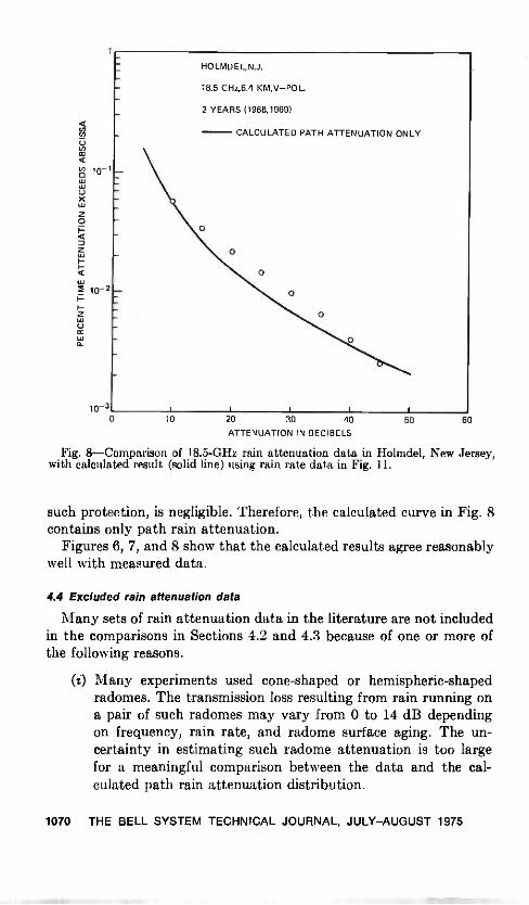
(.7)
10-1
X
017.
E 10-2
I -
w(.)ccwa.
HOLMDEL,N.J.
18.5 GHz,6.4 KM,V-POL.
2 YEARS (1968,1969)
CALCULATED PATH ATTENUATION ONLY
10 20 30 40
ATTENUATION IN DECIBELS
50 60
Fig. 8-Comparison of 18.5-GHz rain attenuation data in Holmdel, New Jersey,with calculated result (solid line) using rain rate data in Fig. 11.
such protection, is negligible. Therefore, the calculated curve in Fig. 8contains only path rain attenuation.
Figures 6, 7, and 8 show that the calculated results agree reasonablywell with measured data.
4.4 Excluded rain attenuation data
Many sets of rain attenuation data in the literature are not includedin the comparisons in Sections 4.2 and 4.3 because of one or more ofthe following reasons.
(i) Many experiments used cone -shaped or hemispheric -shapedradomes. The transmission loss resulting from rain running ona pair of such radomes may vary from 0 to 14 dB dependingon frequency, rain rate, and radome surface aging. The un-certainty in estimating such radome attenuation is too largefor a meaningful comparison between the data and the cal-culated path rain attenuation distribution.
1070 THE BELL SYSTEM TECHNICAL JOURNAL, JULY-AUGUST 1975

(ii) The antennas in the experiment are not covered by anyradomes, exposing the antenna feeds and reflecting surfacesto rain, snow, and ice. No information is available for esti-mating the possible transmission loss from the wetting of theseelements.
(iii) The published information does not specify whether theantennas are covered by radomes or not. The configurationof the radome, if used, is also unknown.
(iv) The polarization of the transmitted signal is unstated.(v) The time base of the experiment is too short to yield long-term
representative statistics.(vi) No rain rate data with T < 2 min is available at or near the
location of the rain attenuation experiment.
V. OUTAGE ESTIMATION FOR 11- AND 18-GHz RADIO LINKS
For a constant transmitter output power, the dependence of fademargin Fo(L) in dB on the path length L is
Fo(L) = Fo(Lo) - 20 logio .170 ) dB, (47)
where Lo is a reference repeater spacing and Fo(Lo) is the correspondingreference fade margin. For 11- and 18-GHz radio, reasonable clear -dayreference fade margins are
Fo = 40 dB for 18 GHz at Lo= 4 kmand
Fo = 40 dB for 11 GHz at Lo = 40 km.
A radio outage occurs when the path rain attenuation plus the wetradome attenuation exceeds the clear -day fade margin Fo. By sub-stituting the fade margin (47) into the attenuation distribution (1), wecan calculate the probability of radio outage per hop as a function ofrepeater spacing L. As an example, Fig. 9 shows the outage probabili-ties' for 11- and 18-GHz radio links in Atlanta, Georgia.
The wet radome attenuation A R is assumed to be 3 dB in these cal-culations of outage probabilities.
VI. SOME QUALIFICATIONS
This section discusses some limitations, approximations, and assump-tions in the theoretical calculation procedure, the data employed, andthe calculated results.
Multipath interference fading can also cause outages. An empirical formula forestimating the multipath-caused outage probability can be found in Ref. 41.
RAIN ATTENUATION 1071
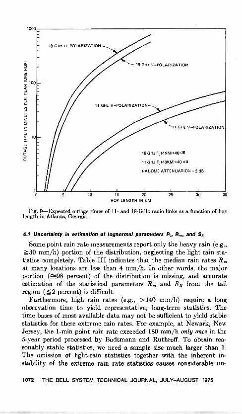
1000
O
0100
cc
>-
cc
10I-LL,
0
18 GHz H-POLARIZATION--_,
18 GHz V-POLARIZATION
11 GHz H-POLARIZATION--,
'11 GHz V-POLARIZATION
18 GHz F.(4KM)=40 dB
11 GHz F0(40KM)=40 dB
RADOME ATTENUATION = 3 dB
0 5 10 15 20
HOP LENGTH IN KM25 30 35
Fig. 9-Expected outage times of 11- and 18-GHz radio links as a function of hoplength in Atlanta, Georgia.
6.1 Uncertainty in estimation of lognormal parameters P., Rm, and SR
Some point rain rate measurements report only the heavy rain (e.g.,30 mm/h) portion of the distribution, neglecting the light rain sta-
tistics completely. Table III indicates that the median rain rates R.at many locations are less than 4 mm/h. In other words, the majorportion (-='98 percent) of the distribution is missing, and accurateestimation of the statistical parameters R, and SR from the tailregion (< 2 percent) is difficult.
Furthermore, high rain rates (e.g., >140 mm/h) require a longobservation time to yield representative, long-term statistics. Thetime bases of most available data may not be sufficient to yield stablestatistics for these extreme rain rates. For example, at Newark, NewJersey, the 1 -min point rain rate exceeded 180 mm/h only once in the5 -year period processed by Bodtmann and Ruthroff. To obtain rea-sonably stable statistics, we need a sample size much larger than 1.The omission of light -rain statistics together with the inherent in-stability of the extreme rain rate statistics causes considerable un-
1072 THE BELL SYSTEM TECHNICAL JOURNAL, JULY-AUGUST 1975

certainty in the estimation of Po, R., and SR. This uncertainty canbe reduced significantly if the light rain portion of the distribution isalso measured and reported.
6.2 Path length dependence of Po
The empirical formula (20) for the dependence of Po on path lengthL is obtained from the rain -gauge network data in Florida. The testof the applicability of this empirical formula to other locations andthe improvement of this approximation will require further multiplerain gauge experiments at other locations.
6.3 Dependence of point rain rate distribution on rain gauge integration time
The dependence of the point rain rate distribution on rain -gaugeintegration time T has been obtained by Bodtmann and Ruthroff"from a 2 -year experiment at Holmdel, New Jersey. Since a 2 -year timebase may not be sufficient to yield stable statistics for high rain rates,a longer time base may be needed to improve this empirical conversionfactor. The applicability of this result to other geographic locationsalso remains to be verified.
6.4 Radome problem
In the comparisons of calculated and measured rain attenuationdistributions, the wet radome attenuations are assumed values. Toimprove this approximation, a more systematic experimental study onthe dependence of radome attenuation on rain rate is needed.
6.5 Anisotropic spatial correlation 11,
At some geographic locations, the squall lines of heavy rain mayhave a predominant orientation related to the predominant orienta-tion of weather fronts."-" This means the spatial correlation # maydepend not only on the spacing but also on the orientation. However,the presently available information is not sufficient for a quantitativedescription of such an anisotropic correlation. Therefore, we use theisotropic correlation coefficient (35) throughout our theoretical cal-culations. Some of the difference between calculated and measuredattenuation distributions may be caused by neglecting the anisotropyof the spatial correlation function.
VII. CONCLUSION
By using lognormal approximations, we have described a methodfor calculating rain attenuation distributions on microwave paths.The calculated results agree reasonably well with experimental datain Massachusetts, New Jersey, and Georgia. This procedure may
RAIN ATTENUATION 1073

prove useful for the design of radio paths using frequencies above 10GHz. To demonstrate the application, Fig. 9 shows the calculatedoutage probability as a function of repeater spacing for 11- and 18-GHzradio links in Georgia.
VIII. ACKNOWLEDGMENTS
I wish to express appreciation to K. A. Jarett who has helped indeveloping a computer program for the numerical calculations in thispaper; to N. Levine, E. E. Muller, W. T. Barnett, D. C. Hogg, A. A. M.Saleh, and T. S. Chu for valuable comments and suggestions thatgreatly improved the consistency and precision of this analysis; toD. C. Hogg, R. A. Semplak, R. A. Desmond, A. E. Freeny, and J. D.Gabbe for rain rate and attenuation data at Holmdel; to W. T.Barnett, M. V. Pursley, and H. J. Bergmann for attenuation datain Georgia; to G. H. Lentz and J. J. Kenny for rain rate and attenua-tion data in Massachusetts; and to C. L. Ruthroff, W. F. Bodtmann,and A. L. Sims for rain rate data at many locations.
APPENDIX A
Derivation of Formulas Relating Rain Attenuation Distribution to Path Length
Since the random fluctuations of the attenuation gradient i (s) atvarious positions in the radio path are partially correlated, we requirethe spatial covariance function of 0 to relate the variance of 0 to thevariance of the path attenuation a. However, raining intervals atseparated observation points are not always coincident. Hence,definition of the spatial covariance function for 0 requires a time basefor all f3s common to all observations. A natural common time basefulfilling this requirement is the total time, including both raining andnonraining intervals. This means the unconditional* statistical meansand variances of 0 and a are also needed in this formulation. We there-fore define
andiiu = E.{0(t)} (48)
_2
.A. = E. { 02 (t) } - Nu (49)
as the unconditional mean and variance, respectively, of j3, whereEu{ } denotes the (unconditional) statistical average including bothraining and nonraining time. We assume that, on a long-term basis,ti. and (IL are independent of position in or near the radio path of
Fading caused by other atmospheric effects, such as multipath interference and"earth -bulge," is not treated in this paper. Therefore, the path rain attenuation aand the attenuation gradient ft are taken to be identically zero during nonrainingtime.
1074 THE BELL SYSTEM TECHNICAL JOURNAL, JULY-AUGUST 1975

au = 5uL.Substituting eqs. (6) and (56) into definition (51) yields
IL L
clu Eu h Q(z) .1(2(z) J J. Q(z')
X ff13(s, 1) 0 (s' , t) dvdv'} - IT:. L2eczi)
= L 1 iJO Q(z) LI(z) f foL Q(z')
interest; therefore, we omit the position argument(s) in eqs. (48) and(49). Similarly,
au = Eu{ct(t)} (50)
ol, = E 2, {a2 (t)} - au (51)
are the unconditional mean and variance, respectively, of a.Based upon the definitions (48) to (51) and the relationships (22)
to (29), it can be shown that conditional and unconditional meansand variances are related by
5 = 5/Po(0) (52)
a = au/Po(L) (53)
SA = In fro(0) [1 + 6' ]} (54)Nu
and
S: = In fro(L) [1 + a . ,--27 i 1 . (55)
Obtaining the unconditional statistical averages of both sides of eq.(6) yields
(56)
X f f { E.D3 (s, 02
13(s', t)] - flu ) dvdv' . (57)
Let us define a spatial covariance function"," Cs(s, s') for 13(s, t) and13(s', 0 such that
CO (S, s') = Eul0(s, 0 g(s', t)} - Su. (58)
In other words,(S')
#u (s) s') =Co , S (59)
13u
is the (spatial) correlation coefficient3435 between 0(s, t) and 11(s1, t).Substituting definitions (58) and (59) into (57) yields
oiu = atiu L2. H (L), (60)
RAIN ATTENUATION 1075
where
H (L)12
= foLQ(z)
fe2 foL (1z,) fQ f%t/u (S, s')dvdv' . (61)
Substituting (56) and (60) into (55) gives2
82(L) = In Po (L) [1 H (L) 134 ]flu
Combining (54) and (62) gives
SRL) = In Po (L) {1 H (L) exP (4 1[Po(0)
Combining eqs. (24), (25), (52), (53), and (56) gives
am(L) = 7. L P°(0) exp [2
-2 8"Po(L)
This completes the derivation for 8:,(L) and an, (L).
APPENDIX B
(62)
(63)
(64)
Lognormal Distribution of Point Rain Rate
Figures 10 to 13 display the distributions of 2-s point rain rateobserved in Miami, Florida; Urbana, Illinois; Atlanta and Palmetto,Georgia; Merrimack Valley, Massachusetts; Holmdel, New Jersey;and Southern England. The time bases range from 1 to 6 years. It canbe seen that these distributions of 2-s point rain rate are very close tothe lognormal approximation in the range below 100 mm/h. The rainrates beyond 100 mm/h are generally separated by more than 3 sigmafrom the median, and constitute the tail of the lognormal distribution.A very long observation time (e.g., more than 20 years) is necessaryto obtain stable statistics of extreme rain rates beyond 100 mm/h.45-48Since the time bases of the data in Figs. 10 to 13 are much less than20 years, the deviations of the data from the lognormal distributionsin the tails are not unexpected.
The rain gauge integration time T in the original data range from1.5 s to 2 min, depending upon the source. As discussed in Section 2.3,the appropriate integration time T, corresponding to 1-m3 samplingvolume in our formulation, is about 2 s. From 2 -year experimentaldata at Holmdel, New Jersey, Bodtmann and Ruthroff" have obtainedan empirical relationship for the dependence of point rain rate dis-tributions on rain gauge integration t time in the range
1.5 s < T < 120 s. (65)
This empirical result enables us to convert the original data into the2-s point rain rate distributions shown in Figs. 10 to 13.
1076 THE BELL SYSTEM TECHNICAL JOURNAL, JULY-AUGUST 1975

5
10-1
lo -2
10-3
10 4
RAIN GAUGE INTEGRATION TIME T=2 SECONDS
0 3 YEARS (5/69-4/72)
3 YEARS (1971-1973)
A 4 YEARS (5/61-5/62,63,70,71)
LOGNORMAL APPROXIMATION
SOUTHERNENGLAND
0 URBANA,I LL.
MERRIMACK VALLEY, MASS.
0 40 80 120 160
RAIN RATE IN mm/h
200 240
Fig. 10-Lognormal distribution of 2-s point rain rate at Urbana, Illinois; Merri-mack Valley, Massachusetts; and Southern England.
APPENDIX C
Derivation for Path Length Dependence of PO(L)
Let Po(L1) and Po(Li + AL) be the probabilities that rain falls onthe radio path with length L1 and an extended path of length L1 + AL,
where AL is a small incremental length. The relation between Po(Li)
RAIN ATTENUATION 1077
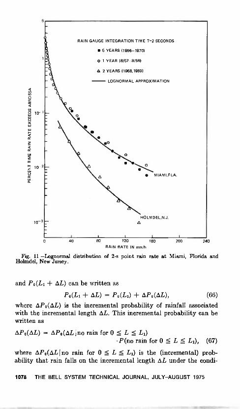
5
U)
U)co
cf)
10-1
cc
rtcc
10-2
ccw.
10-2
RAIN GAUGE INTEGRATION TIME T=2 SECONDS
5 YEARS (1966-1970)
O 1 YEAR (8/57-8/58)
O 2 YEARS (1968,1969)
LOGNORMAL APPROXIMATION
MIAMI,FLA.
HOLMDEL,N.J.
0 40 80 120 160
RAIN RATE IN mm/h200 240
Fig. 11-Lognormal distribution of 2-s point rain rate at Miami, Florida andHolmdel, New Jersey.
and Po (L1 + AL) can be written as
Po(Li + AL) = Po(Li) AP0(AL), (66)
where APo(AL) is the incremental probability of rainfall associatedwith the incremental length L. This incremental probability can bewritten as
AP0(AL) = AP0(AL I no rain for 0 < L < L1)P(no rain for 0 < L < L1), (67)
where AP0(AL I no rain for 0 L L1) is the (incremental) prob-ability that rain falls on the incremental length AL under the condi-
1078 THE BELL SYSTEM TECHNICAL JOURNAL, JULY-AUGUST 1975
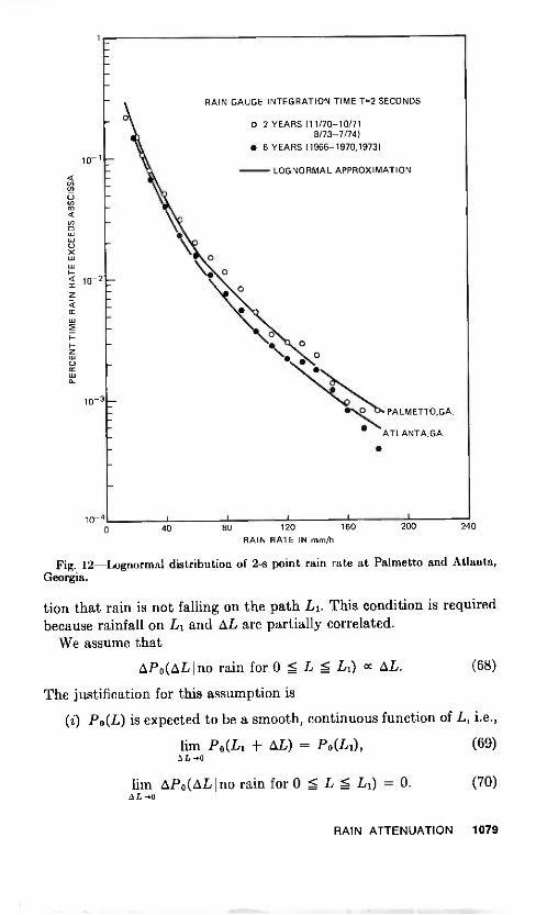
0-1
10-2
io-3
RAIN GAUGE INTEGRATION TIME T=2 SECONDS
o 2 YEARS (11/70-10/718/73-7/74)
6 YEARS (1966-1970,1973)
LOGNORMAL APPROXIMATION
o
Oo
PALMETTO,GA.
4DATLANTA,GA.
10-4040 80 120 160
RAIN RATE IN mm/h200 240
Fig. 12-Lognormal distribution of 2-s point rain rate at Palmetto and Atlanta,Georgia.
tion that rain is not falling on the path L1. This condition is requiredbecause rainfall on L1 and AL are partially correlated.
We assume that
AP0(AL I no rain for 0 < L < L1) oc AL. (68)
The justification for this assumption is
(i) Po(L) is expected to be a smooth, continuous function of L, i.e.,
lim Po(LI + AL) = Po(Li), (69)AL -.0
lira APo(AL no rain for 0 5 L < L1) = 0. (70)AL -.0
RAIN ATTENUATION 1079
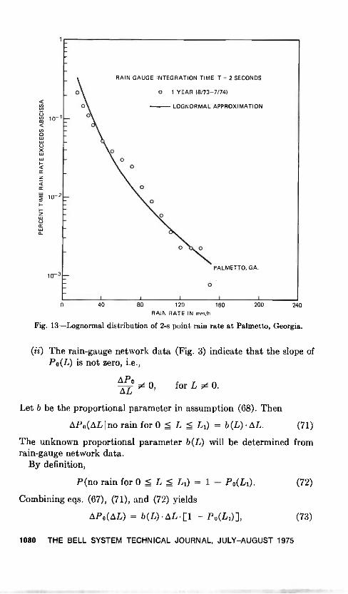
10-1
10-2
10-3
RAIN GAUGE INTEGRATION TIME T = 2 SECONDS
0 1 YEAR (8/73-7/74)
LOGNORMAL APPROXIMATION
O
O
PALMETTO, GA.
0 40 80 120 160
RAIN RATE IN mm/h200 240
Fig. 13-Lognormal distribution of 2-s point rain rate at Palmetto, Georgia.
(ii) The rain -gauge network data (Fig. 3) indicate that the slope ofPo(L) is not zero, i.e.,
APoAL
0' for L O.
Let b be the proportional parameter in assumption (68). Then
AP0(AL I no rain for 0 < L < L1) = b(L) AL. (71)
The unknown proportional parameter b (L) will be determined fromrain -gauge network data.
By definition,
P(no rain for 0 L1) = 1 - Po(Li) (72)
Combining eqs. (67), (71), and (72) yields
AP0(AL) = b(L)ALEl - Po(Lin,
1080 THE BELL SYSTEM TECHNICAL JOURNAL, JULY-AUGUST 1975
(73)
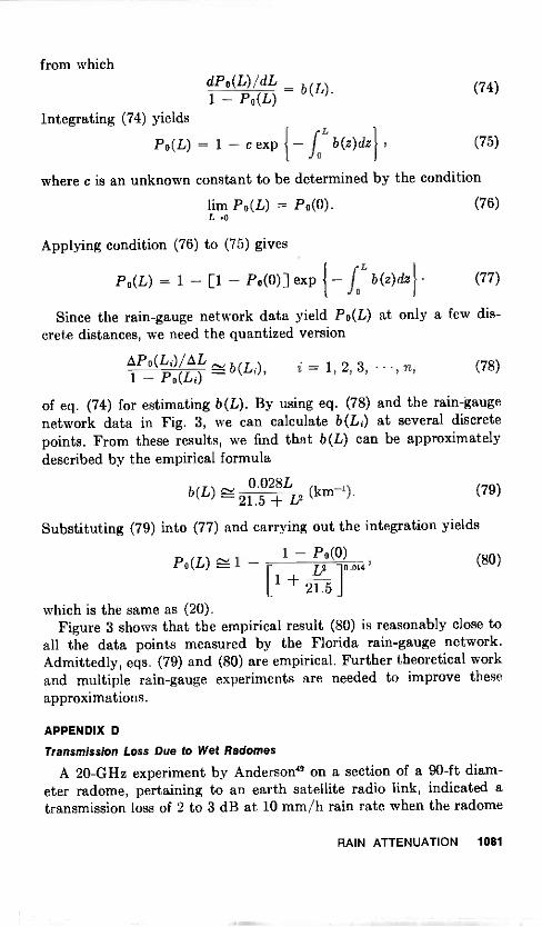
from whichdP (L) / dL = b(L). (74)1 - Po(L)
Integrating (74) yieldsL
Po(L) = 1 - c exp - b(z)dz} (75)
where c is an unknown constant to be determined by the condition
lim Po(L) = Po(0).L
Applying condition (76) to (75) gives
(76)
Po(L) = 1 - [1 - Po(0)] exp -J
L b(z)dzi (77)
Since the rain -gauge network data yield Po(L) at only a few dis-crete distances, we need the quantized version
AP o(Li)/ ALb (L i) = 1, 2, 3, - , n, (78)
1 - Po( L i) '
of eq. (74) for estimating b(L). By using eq. (78) and the rain -gaugenetwork data in Fig. 3, we can calculate b(Li) at several discretepoints. From these results, we find that b(L) can be approximatelydescribed by the
b(L) - 0.028E(km -1). (79)
21.5 + L2
Substituting (79) into (77) and carrying out the integration yields
1 - Po(0)Po(L) 1 (80)L2 0.014 2
121.5
which is the same as (20).Figure 3 shows that the empirical result (80) is reasonably close to
all the data points measured by the Florida rain -gauge network.Admittedly, eqs. (79) and (80) are empirical. Further theoretical workand multiple rain -gauge experiments are needed to improve theseapproximations.
APPENDIX D
Transmission Loss Due to Wet Radomes
A 20-GHz experiment by Anderson" on a section of a 90 -ft diam-eter radome, pertaining to an earth satellite radio link, indicated atransmission loss of 2 to 3 dB at 10 mm/h rain rate when the radome
RAIN ATTENUATION 1081

was new. However, after 6 months of weathering, the transmissionloss increased to 8 dB at 10 mm/h rain rate. A 4-GHz experiment50on an earth -satellite radio link indicated a 3 -dB transmission loss re-sulting from the wet radome. These experimental data agree rea-sonably well with theoretical calculations"-" for rain rates < 10 mm/h,assuming laminar water flow on hemispherical radome surface pointingtowards the zenith.
For typical 11- and 18-GHz terrestrial radio paths, the transmissionlosses from wet radomes are expected to be smaller than those of earth -
satellite radio links because of the smaller radome size, differentradome shape, and orientation. However, the terrestrial radio passesthrough a pair of radomes on each link; therefore, the contribution ofwet radome loss to the total path attenuation may not be negligible.Theoretical calculation of wet radome attenuation pertaining toterrestrial radio links is not available at the present time because ofthe difficulty in calculating the nonuniform thickness of the water film.A semiquantitative experiment" was carried out on the 12.2-GHz radiolink between Murray Hill and Crawford Hill, New Jersey (22 miles).The 10 -ft dish antenna was covered by a cone -shaped radome thatwas made of resin -coated fiberglass and, at 10 years of age, was wellweathered. Water was sprayed on the radome-covered antenna by amanually controlled sprinkler. The results indicated that a uniformlight sprinkle caused approximately 2.5 -dB attenuation, whereas avery heavy spray (maximum stream of water) caused between 4- and7 -dB attenuation. After the spray was turned off, 2 to 3 minuteselapsed before the signal recovered to within 1 dB of its nonfaded level.The residual wet radome attenuation is estimated to be 0.5 dB.
On an 18-GHz, 4.3 -km path at Merrimack Valley, Massachusetts,Kenny" has also observed a residual wet radome attenuation of 0.75dB (i.e., 1.5 dB for two radomes).
APPENDIX E
List of Symbols and Their Definitions
A, Collecting aperture of a rain gauge.AR Attenuation by two wet radomes on a radio link.Cp (s, s') Spatial covariance function of /3(s, t) and /3(s', t) as de-
fined by eq. (58).dv = pdpdOdz.E LI ^, Conditional statistical (time) average under the condition
that the point rain rates, in the radio path of length L(see Fig. 1), are not all zero.
1082 THE BELL SYSTEM TECHNICAL JOURNAL, JULY-AUGUST 1975

Conditional statistical (time) average under the conditionthat the point rain rate (defined in Section 2.3) is notzero at the position of interest.
Unconditional statistical (time) average including bothraining and nonraining time.
erf Complementary error function.Fo Fade margin of radio links.G Characteristic distance defined in eq. (35). See also Sec-
tion 4.1.h (z) Radius of the circular cross section of radio beam at a
distance z from the transmitter. See Fig. 1 and eq. (3).H (L) Defined by eqs. (32) and (36).H-Pol Horizontal polarization.L The path length of a radio link ; see Fig. 1.Lo A reference repeater spacing defined by eq. (47).In Natural logarithm.P (a > A) Probability that rain attenuation a exceeds A.P (R > r) Probability that rain rate R exceeds r.P B) Probability that attenuation gradient 13 exceeds B.P o(L) Probability that rain is falling on a radio link of length L.Po(0) = ; the probability that rain is falling at the
position of interest.Q (z) = 7/12 (z) area of the circular cross section of radio beam
at a distance z from the transmitter. See eqs. (3) and (4).R (s, Point rain rate measured by a 1-m3 sampling volume
located at s.Median value of the point rain rate R during raining time.
s A vector to denote the position (p, 445, z).8,, Standard deviation of In a during raining time.SR Standard deviation of In R during raining time.S Standard deviation of In during raining time.T Integration time of rain gauge.t Time.TAY Defined in eq. (10).V-Pol Vertical polarization.V R Average falling velocity of raindrops.A V Incremental sampling volume for measurement of point
rain rate. See Section 2.3.z Distance from the radio transmitter (Fig. 1).a Rain attenuation in decibels.am Median value of a during raining time.a Mean value of a during raining time.
RAIN ATTENUATION 1083

au Unconditional statistical mean of a as defined by eq. (50).0 Point rain attenuation gradient measured in dB/km by a
1-m3 sampling volume as discussed in Section 2.3.(3m Median value of (3 during raining time.
Mean value of during raining time.0,(z, Average of 0(s, t) over the circular cross section Q of the
radio beam. See eqs. (5) and (7).Unconditional statistical mean of (3 as defined by eq. (48).= -(1)'.A parameter defined by eq. (12) relating point rain atten-
uation gradient (3 and point rain rate R.X Radio wavelength.
A parameter defined by eq. (12) relating point rain atten-uation gradient 0 and point rain rate R.
as Standard deviation of a during raining time.(Tau Unconditional standard deviation of a as defined by
eq. (51).Standard deviation of 3 during raining time.
a(3u Unconditional standard deviation of as defined byeq. (49).
p Radial distance from the z-axis in the cylindrical co-ordinate system in Fig. 1.
4) Angle in the cylindrical coordinate system in Fig. 1.¢u (s, s') Correlation coefficient between 0(s, t) and fl (s', t) as
defined by eqs. (33) and (59).
REFERENCES
1. A. E. Freeny and J. D. Gabbe, "A Statistical Description of Intense Rainfall,"B.S.T.J., 48, No. 6 (July -August 1969), pp. 1789-1851.
2. A. E. Freeny and J. D. Gabbe, private communication.3. D. C. Hogg, "Statistics on Attenuation of Microwaves by Intense Rain,"
B.S.T.J., 48, No. 9 (November 1969), pp. 2949-2962.4. C. R. Stracca, "Propagation Tests of 11 GHz and 18 GHz on Two Paths of
Difference Length," Alta Frequenza, Italy, 38, 1969, pp. 345-360.5. D. C. Hogg, "Path Diversity in Propagation of Millimeter Waves Through
Rain," IEEE Trans. Ant. Prop., AP -15, No. 3 (May 1967), pp. 410-415.6. S. H. Lin, "Statistical Behavior of Rain Attenuation," B.S.T.J., 52, No. 4 (April
1973), pp. 557-581.7. J. A. Morrison, M. J. Cross, and T. S. Chu, "Rain -Induced Differential Attenua-
tion and Differential Phase Shift at Microwave Frequencies," B.S.T.J., 52,No. 4 (April 1973), pp. 599-604.
8. T. Oguchi, "Attenuation and Phase Rotation of Radio Waves due to Rain :Calculation at 19.3 and 34.8 GHz," Radio Science, 8, No. 1 (January 1973),pp. 31-38.
9. R. G. Medhurst, "Rainfall Attenuation of Centimeter Waves: Comparison ofTheory and Measurement," IEEE Trans. Ant. Prop., AP -13, No. 4 (July1965), pp. 550-564.
10. D. E. Setzer, "Computed Transmission Through Rain at Microwave and VisibleFrequencies," B.S.T.J., 4.9, No. 8 (October 1970), pp. 1873-1892.
1084 THE BELL SYSTEM TECHNICAL JOURNAL, JULY -AUGUST 1975

11. J. W. Ryde, "Echo Intensity and Attenuation due to Clouds, Rain, Hail ; Sandand Dust Storms at Centimeter Wavelength," Report 7831, General ElectricCompany Research Laboratories, Wembly, England, October 1941.
12. D. Ryde and J. W. Ryde, "Attenuation of Centimeter Waves by Rain, Hail andClouds," Report 8516, General Electric Company Research Laboratories,Wembly, England, August 1944.
13. D. Ryde and J. W. Ryde, "Attenuation of Centimeter and Millimeter Waves byRain, Hail, Fogs and Clouds," Report 8670, General Electric Company Re-search Laboratories, Wembly, England, May 1945.
14. D. M. A. Jones and A. L. Sims, "Climatology of Instantaneous PrecipitationRates," Illinois State Water Survey at the University of Illinois, Urbana,Illinois. Project No. 8624, Final Report, December 1971.
15. W. F. Bodtmann and C. L. Ruthroff, "Rain Attenuation on Short Radio Paths :Theory, Experiment, and Design," B.S.T.J., 53, No. 7 (September 1974),pp. 1329-1349.
16. J. R. Norbury and W. J. K. White, "Point Rainfall Rate Measurements atSlogh, U.K.," Conference on Propagation of Radio Waves at Frequenciesabove 10 GHz, April 10-13, 1973, London, England, Conference Records, pp.190-196 and IEE (London) Conference Publication Number 98.
17. B. J. Easterbrook and D. Turner, "Predication of Attenuation by Rainfall in the10.7-11 GHz Communication Band," Proc IEE (London), 114, No. 5, (May1967), pp. 557-565.
18. K. Funakawa and J. Kato, "Experimental Studies of Propagational Characteris-tics of 8.6-m Wave on the 24 -km Path," J. Radio Research Labs (Japan),9, No. 45 (September 1962), pp. 351-367.
19. K. Moritta and I. Higuti, "Statistical Studies on Electromagnetic Wave Attenua-tion Due to Rain," Review of the Electrical Communication Laboratories(Japan), 19, No. 7-8 (July -August 1971), pp. 798-892.
20. A. L. Sims and D. M. A. Jones, "Climatology of Instantaneous PrecipitationRates," Illinois State Water Survey at the University of Illinois, Urbana,Illinois. Project No. 8624, March 1973.
21. C. L. Ruthroff, "Rain Attenuation and Radio Path Design," B.S.T.J., 49, No. 1(January 1970), pp. 121-135.
22. E. A. Mueller and A. L. Sims, "Investigation on the Quantitative Determinationof Point and Areal Precipitation by Radar Echo Measurement," TechnicalReport ECOM-00032-F, Illinois State Water Survey at the University ofIllinois, Urbana, Illinois, December 1966.
23. D. C. Hogg, "How the Rain Falls," unpublished work.24. R. A. Semplak and R. H. Turrin, "Some Measurements of Attenuation by
Rainfall at 18.5 GHz," B.S.T.J., 48, No. 6 (July -August 1969), pp. 1767-1787and Figure 11.
25. E. A. Mueller and A. L. Sims, "The Influence of Sampling Volume on RaindropSize Spectra," Proc. Twelfth Conference on Radar Meterology, AmericanMeteorological Society, October 1966, pp. 135-141.
26. J. 0. Laws and D. A. Parsons, "The Relation of Rain Drop Size to Intensity,"Trans. Am. Geophysical Union, 25, 1943, pp. 452-460.
27. J. A. Morrison and M. J. Cross, "Scattering of a Plane Electromagnetic Wave byAxisymmetric Raindrops," B.S.T.J., 53, No. 6 (July -August 1974), pp. 955-1020.
28. T. S. Chu, private communications.29. T. S. Chu, "Rain Induced Cross Polarization at Centimeter and Millimeter
Wavelength," B.S.T.J., 53, No. 8 (October 1974), pp. 1557-1579.30. W. T. Barnett, "Some Experimental Results on 18 GHz Propagation," The
1972 National Telecommunications Conference, December 4-6, 1972, IEEE,Houston, Texas, Conference Record, pp. 10E -1-10E4 and IEEE Publication72 CHO 601-5-NTC.
31. R. A. Semplak, "Effect of Oblate Raindrops on Attenuation at 30.9 GHz,"Radio Science, 5, No. 3 (March 1970), pp. 559-564.
32. Local Climatological Data, U. S. Department of Commerce, EnvironmentalScience Services Administration, National Weather Records Center, Ashville,North Carolina, 28801. Also available from Superintendent of Documents,U. S. Government Printing Office, Washington, D. C. 20402.
33. J. Aitchison and J. A. C. Brown, The Lognormal Distribution, London : CambridgeUniversity Press, 1957.
RAIN ATTENUATION 1085

34. A. Papoulis, Probability, Random Variables, and Stochastic Processes, New York :McGraw-Hill, 1965, pp. 210 and 282.
35. P. Beckmann, Probability in Communication Engineering, New York : Harcourt,Brace and World, 1967, pp. 88 and 204.
36. G. H. Lentz and J. J. Kenny, private communication.37. W. T. Barnett, H. J. Bergmann, and M. V. Pursley, private communication.38. R. A. Semplak, "The Influence of Heavy Rainfall on Attenuation at 18.5 GHz
and 30.9 GHz," IEEE Trans. Ant. Prop., AP -18, No. 4 (July 1970), pp.507-511.
39. B. N. Harden, J. R. Norbury, and W. J. K. White, "Model of Intense ConvectiveRain Cells For Estimating Attenuation on Terrestrial Millimetric RadioLinks," Elec. Letters, 10, No. 23 (November 1974), pp. 483-484.
40. D. C. Hogg, "Intensity and Extent of Rain on Earth -Space Paths," Nature, 2.48,June 8, 1973, pp. 337-338.
41. W. T. Barnett, "Multipath Propagation at 4, 6, and 11 GHz," B.S.T.J., 51, No. 2(February 1972), pp. 321-361.
42. R. R. Braham, Jr., and H. R. Byers, The Thunderstorms, Report of the Thunder-storm Project, Government Printing Office, Washington, D. C., 1949, ChapterVIII Squall Lines.
43. R. J. Boucher and R. Wexler, "The Motion and Predictability of PrecipitationLines," J. Meteorology, 18, No. 2 (April 1961), pp. 160-171.
44. D. A. Gray, "Earth -Space Path Diversity Dependence on Base Line Orientation,"1973 International IEEE/G-AP Symposium and URSI Meeting, Boulder,Colorado, August 1973, Symposium Record pp. 366-369.
45. "Rainfall Intensity -Duration -Frequency Curves for Selected Stations in theUnited States, Alaska, Hawaiian Islands, and Puerto Rico," Weather Bureau,U. S. Department of Commerce, Tech. Paper 25, December 1955.
46. L. H. Seamon and G. S. Bartlett, "Climatological Extremes," Weatherwise, 9,1956, pp. 194-213.
47. A. E. Cole, R. J. Donaldson, R. Dyer, A. J. Kantor and R. A. Skrivanek, "Pre-cipitation and Clouds, a Revision of Chapter 5, Handbook of Geophysics andSpace Environments," AFCRL-69-0487, Air Force Surveys in Geophysics,No. 212, Office of Aerospace Research, U.S. Air Force Cambridge ResearchLaboratories, Bedford, Massachusetts, November 1969.
48. W. Y. S. Chen, private communication.49. I. Anderson, "Measurements of 20 GHz Transmission Through a Wet Radome,"
1973 International IEEE/G-AP Symposium and URSI Meeting, Boulder,Colorado, August 1973, Symposium Record, pp. 239-240.
50. A. J. Giger, "4-gc Transmission Degradation Due to Rain at Andover, Maine,Satellite Station," B.S.T.J., 44, No. 7 (September 1965), pp. 1528-1533.
51. A. Cohen and A. Smolski, "The Effect of Rain on Satellite CommunicationsEarth Terminal Rigid Radomes," Microwave J., 9, No. 9 (September 1966),pp. 111-121.
52. D. Gibble, "Effects of Rain on Transmission Performance of a Satellite Com-munication System," IEEE International Convention Record, Part VI,March 1964, p. 52.
53. B. Blevis, "Losses Due to Rain on Radomes and Antenna Reflecting Surfaces,"IEEE Trans. Ant. Prop., AP -13, No. 1 (January 1965), pp. 175-176.
54. B. Blevis, "Rain Effects on Radomes and Antenna Reflectors," Proc. IEE Con-ference on Large Steerable Aerials, London, 1966, pp. 148-152.
55. H. J. Bergmann and S. H. Lin, "Measurements of 12 GHz Transmission LossThrough a Wet Radome," unpublished work.
1086 THE BELL SYSTEM TECHNICAL JOURNAL, JULY -AUGUST 1975

Copyright 1975 American Telephone and Telegraph CompanyTHE BELL SYSTEM TECHNICAL JOURNAL
Vol. 54, No. 6, July -August 1975Printed in U.S.A.
A Geometric Derivation of Forney'sUpper Bound
By J. E. MAZO
(Manuscript received January 17, 1975)
Effective analyses of performance for detection schemes that optimallydecode digital data in the presence of intersymbol interference have beenslow in coming. Recently, however, Forney has given an upper bound onthe bit error probability for maximum -likelihood sequence estimation.Starting from a standard geometrical framework, we give a much simplifiedderivation of this upper bound. Our derivation places the validity of thisimportant bound more in evidence in that the concepts of whitened matchedfilter and error event are not introduced.
Let ai, j = 1, 2, , N, be independent, equilikely binary randomvariables taking values ±1. Data transmission usually involvesestimating the ai from a pulse sequence of the form
Na ih (t - jT), - < t < 00, (1)
J-1
which is observed in white gaussian noise of (two-sided) spectraldensity No/2. In (1), the minimum assumption put on the pulse wave-form h (t) is that it be L2. One possible detection procedure is to decide,on the basis of the received noisy signal, which one of the 2N equilikelysignals given in (1) was "most likely" (maximum -likelihood sequencedetection) and use the sequence fan which is associated with thatsequence as the detected symbols. As N grows large, the probability ofdeciding incorrectly on the sequence approaches unity; however, thereal question revolves about the bit -error probability for maximum-likelihood sequence detection. Important work on this problem wasdone recently by Forney,1.2 who showed that, under certain conditionson h(t), the bit -error probability for large signal-to-noise ratios goes
1087

exponentially to zero asdfnin
Pe ;7:: (coeff.) exp ( -4No ) '
No ---* 0, (2)
where dlin is the minimum distance between the signal sequences in(1) ; i.e., if we add a superscript to distinguish among sequences thus
N.3") (i) = E ar)h(i - jT), -co < t < 00 i = 1, 2, , 2N, (3)
J----1
then,..
dam, = lim min f Isci) (I) - s(k) (012dt.N -). i, k -coilk
(4)
Forney's demonstration consists of two steps. First, a lower bound onPe of the form (2) is established, valid for any h(t). Second, if H(w)denotes the Fourier transform of h (t) and
1 cef I H(w) I 2eikwc/c..) = 0 for integer k, 1kI > V, v integer, (5)
then an upper bound for Pc can be given which is convergent for largesignal-to-noise ratios and which, furthermore, also has an asymptoticform given by (2).
In our opinion, Forney's discussion of the upper bound is sufficientlycomplicated that some question remains as to how firmly the result isestablished. We shall give a much simpler derivation, but first let usreview the situation when v = 0, i.e., when there is no intersymbolinterference. Using the reduction to the standard geometrical picture,'the signal points (sequences) received in the absence of noise are asshown in Fig. 1. These signal points are to be regarded as being per-turbed by spherically symmetric, N -dimensional, zero mean gaussiannoise ; the variance of each component of the noise is N0/2. Thus anypoint in the N -dimensional space may be received and the maximum -likelihood decoder chooses the unperturbed sequence nearest to thereceived point as the transmitted one. The decoding regions are shownin Fig. 2 by dashed lines, and are labeled Ri,j in an obvious way.
Now assume we transmit (1, 1) and ask for the probability that thefirst bit is in error. This is the same as the probability that the receivedsignal point is in R_1,1 U R_1,_1, or equivalently that the receivedsignal point is to the left of the line labeled S in Fig. 1. In N dimensionsit would be the probability that the received signal point is on theopposite side of an (N - 1) dimensional hyperplane. This is clearly asimple one-dimensional gaussian problem having the well-known Q-
1088 THE BELL SYSTEM TECHNICAL JOURNAL, JULY -AUGUST 1975

R-1,1
1
S
R11
R-1-1
-F
1
1
S
L
E.
R1,-1
Fig. 1-Four signal points corresponding to sequences for N = 2 in the absence ofintersymbol interference.
si
I
S
Fig. 2-Four signal points with intersymbol interference.
GEOMETRIC DERIVATION 1089

function for an answer, independent (because of the simple geometry)of the dimension or of which bit in the sequence is transmitted.
When intersymbol interference is present, the error probability forthe kth bit may well depend on k and N. In addition, the surface Swhich separates the sequences that have ak = +1 from those whichhave ak = -1 is no longer a hyperplane, although it is made up ofsegments which are hyperplanes. Finally, and perhaps a bit vaguely,the "shape" of the surface may depend on k. An example for N = 2 isgiven in Fig. 2 showing the separating surface for the first bit.
Our goal is to derive Forney's upper bound by geometrical argumentsabout as simple as those used in the discussion of Fig. 1.
As in (3), we consider signal points identified by their respectivedata sequences fail N and label them with a superscript. We focuson the kth bit being in error, and define sets A and B :
A = law lag) = +1}, B = {am lag) = -1}=----. {b(i)}. (6)
We are mainly interested in the chance that the maximum -likelihooddecoder selects a point b E B, given that a particular sequence a")(say), a") E A, was transmitted. One upper bound on this is the unionbound
d(a"), b)),13 e(k)
b EB ( "SIZ17o i(7)
where d(e), b) is the euclidean distance between en and b ; i.e., if 1labels the particular b sequence,
..,
d2(a 0), b) = 1 I so)(t) - s (z) (t) I2dt-.= f
7-r .1 : I H (w) 12
NE 1a71) - bY))eijw5-1
2
dw. (8)
On writing (8), and henceforth, we set T = 1. Equation (7) is a badbound because it includes too many terms on the right-hand side. Thisis easily seen by applying it to the N -dimensional hypercube (no inter -symbol interference), for which we obtain (ignoring unessentialcoefficients)
Pe(k) < 2N e- - (d2 1 4N o) (9)
where d2 is the length of a hypercube edge. Thus, the bound, for anyfixed No, approaches 00 as the length of the sequence N increases.
Our next step will be to make some simple observations about thegeometry of the received signal points [when (5) is true] that will allowus to delete most of the terms on the right-hand side of (7). Following
1090 THE BELL SYSTEM TECHNICAL JOURNAL JULY -AUGUST 1975

Forney, we are motivated to define another set ./31 of signal pointswhich is a subset of B. A vector b E /31 if { b; - a(;')17=1 (after deletingall zeros which begin the sequence and end the sequence of coefficientsb; - a(l) }) does not contain v or more consecutive zeros either to the
right of the kth position or to the left of the kth position. Forney'supper bound then reads
QCaw, b)
1'e (k)TN'o
(10)
To see why no further terms need be included in (10), select an arbi-trary signal point b* not included in the sum in (10) ; i.e., b* E B- B1 = B*. From the way things have been defined, we may write
act) = 1, al, a2, a3) (11)
b* = -1, gl, az) 53), (12)
where al - (ii does not contain v consecutive zeros in its coefficientsequence and co - g3 0. The 1 in (11) and the ( -1) in (12) occurin the kth position, and «2 is at least of dimension v, corresponding tothe v (or more) positions where a' and b* are to agree. Now al., -may or may not contain v consecutive zeros,t and we distinguish thesetwo cases in our discussion. First assume that al, - 1L does not contain
consecutive zeros. Then note that
(13)
a(2) (cm, 1, at, a2, (33) E A. (14)
Statement (13) is true by the absence of v consecutive zeros in 1L -and also in g, - a1; (14) is true because aP = +1. We may at thispoint imagine the four signal points am, b*, b('), a(2) in general positionas in Fig. 3. Now focus attention on the triangle (a(1), a(2), b*).: Wehave (letting Oi denote a string of at least i zeros)
d2 (am, b*) = Ham - b*ii2=IIaL- 2, at - $i, Ov, a3 - $3112= mat, $L,2, - #1112 iia3 $3112. (15)
The last step in (15) follows from the Fourier integral expression (8)for the distance and from (5), the requirement that intersymbol inter-ference not extend beyond P. The right member of (15) can readilybe seen from (11, 12) and (13, 14) to be d2(a(2), b*) d2 (am , a(2)).
bo.) = (gL, -1, gi, a2, az) E B,
t Recall that a string of zeros in the beginning does not count.We drop bold -face notation for vectors here, and also allow ourselves the freedom
of writing the subscript L as a superscript.
GEOMETRIC DERIVATION 1091
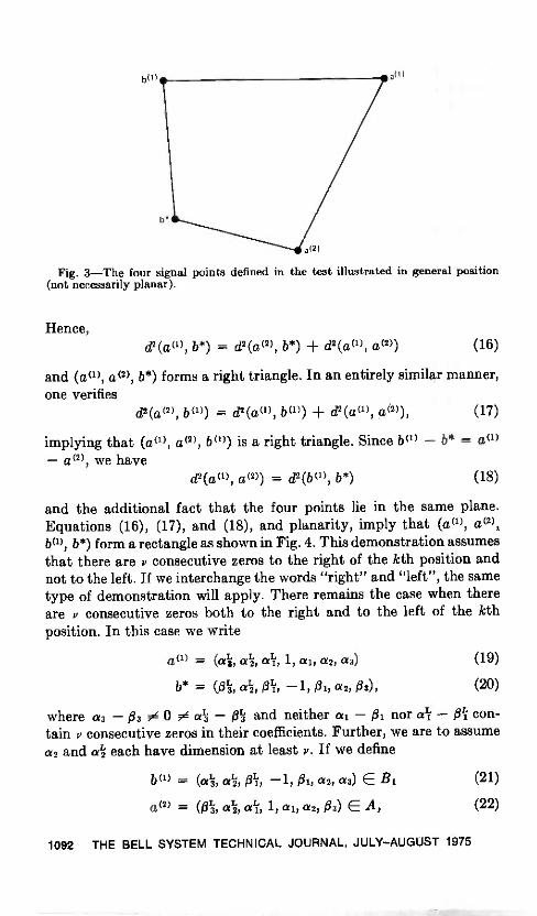
01)
Fig. 3-The four signal points defined in the test illustrated in general position(not necessarily planar).
Hence,d2 (a(i) b*) = d2 (0) b*) ± d2 (am a(2)) (16)
and (0), a(2), b*) forms a right triangle. In an entirely similar manner,one verifies
d2(0), bo)) = d2(ao), ba)) ± d2(a a), a(2)), (17)
implying that (0), e2), b")) is a right triangle. Since b" - b* = ail)- a(2), we have
d2 (au) a(2)) = d2 ow b*) (18)
and the additional fact that the four points lie in the same plane.Equations (16), (17), and (18), and planarity, imply that (am, a(2),b(1) , b*) form a rectangle as shown in Fig. 4. This demonstration assumesthat there are v consecutive zeros to the right of the kth position andnot to the left. If we interchange the words "right" and "left", the sametype of demonstration will apply. There remains the case when thereare v consecutive zeros both to the right and to the left of the kthposition. In this case we write
a(') = (ali, a', a', 1, ai, a2, a3) (19)
b* = (013', aii, 0i, -1, 01, co, $3), (20)
where a3 - 13 0 ali - $ii and neither al - 01 nor all' - 0i con-tain v consecutive zeros in their coefficients. Further, we are to assumea2 and at each have dimension at least P. If we define
VI) = (alg, ali, 1311, -1, /31, a2, a3) E B1 (21)
a(2) = (Qra, «Li, ai, 1, ai, a2, 03) E A, (22)
1092 THE BELL SYSTEM TECHNICAL JOURNAL, JULY-AUGUST 1975

the proof that (a 0), a(2), bo) , b*) is a rectangle can be carried out usingthe same techniques as earlier.
Figure 4 makes it clear why, if a (I) is transmitted, terms like b* donot have to be included in the right-hand side of (10). The term
d(ai , b')
\ 2N 0
in (10) is the probability that, if ail) is transmitted, the received signalwill be on the "wrong side" of the hyperplane H which perpendicularlybisects the line (WO . Now b* only needs to be included in (10) if itsassociated decoding region contributes some set of points of positivemeasure not accounted for in some other way. Thus, from Fig. 4, thisis only the case if these new points were on the same side of H asau). But any point on that side is closer to ace) than b* and, hence,would never be decoded into b*. Hence the gaussian measure of thedecoding region for b* is already included in the term
d(b1 , a')0 /
If we calculate further upper bounds for (10) by letting N = co,we obtain a bound independent of k. Averaging this over the possible
symbols gives precisely Forney's upper bound. The factthat the resulting upper bound converges for No small enough (for
01)
b
H
L.
7 re a(2)
Fig. 4-The actual relationship of the four signal points defined in the text.
GEOMETRIC DERIVATION 1093

N = cc) has been recently discussed by Foschini.4 This last step is animportant one in a full proof, and was overlooked in the initial work.'
REFERENCES
1. G. David Forney, "Lower Bounds on Error Probability in the Presence of LargeIntersymbol Interference," IEEE Trans. Commun., COM-20 (February 1972),pp. 76-77.
2. G. David Forney, "Maximum Likelihood Sequence Estimation of Digital Se-quences in the Presence of Intersymbol Interference," IEEE Trans. Inform.Theory, IT -18 (May 1972), pp. 363-378.
3. J. M. Wozencraft and I. M. Jacobs, Principles of Communication Engineering.New York : John Wiley, 1965, Ch. 4.
4. G. J. Foschini, "Performance Bound for Maximum Likelihood Reception ofDigital Data," IEEE Trans. Inform. Theory, IT -21, No. 1 (January 1975),pp. 47-50.
1094 THE BELL SYSTEM TECHNICAL JOURNAL, JULY -AUGUST 1975

Copyright © 1975 American Telephone and Telegraph CompanyTHE BELL SYSTEM TECHNICAL JOURNAL
Vol. 54, No. 6, July -August 1975Printed in U.S.A.
Power Spectrum of a Digital, Frequency -
Modulation Signal
By H. E. ROWE and V. K. PRABHU(Manuscript received December 31, 1974)
We present the power spectrum of a sinusoidal carrier, frequencymodulated by a random baseband pulse train in which the signaling -pulseduration is finite and the signal pulses may overlap and have differentshapes. Symbols transmitted during different time slots are assumed tobe statistically independent and identically distributed. The spectraldensity appears as a Hermitian form suitable for numerical computationby a digital computer. Simple conditions in terms of the modulationparameters are given under which discrete spectral lines are present in thespectrum. Several examples are given to illustrate the method.
I. INTRODUCTION
In recent years, digital -frequency and phase -modulation techniqueshave been increasingly important in radio, waveguide, and opticalcommunication systems.
An important parameter in the statistical description of a signal isits spectral density, which defines the average power density of thesignal as a function of frequency. In addition to furnishing an estimateof bandwidth requirements, the knowledge of the spectral density isalso essential in the evaluation of mutual interference betweenchannels.
In this paper, we extend the techniques developed in Ref. 1 fordigital PSK to the case of digital FSK with phase -continuous transitions,such as may be obtained at the output of a voltage -controlled oscillatordriven by a digital baseband wave. We assume that the sinusoidalcarrier is frequency modulated by a random, baseband pulse train inwhich the signaling pulse duration is finite and the signal pulses mayoverlap and have different shapes. It is generally assumed that thesymbols transmitted during different time slots are statistically inde-pendent and identically distributed.
We express the spectral density of such an ensemble of continuous -phase, constant -envelope, digital, FM waves as a compact Hermitian
1095
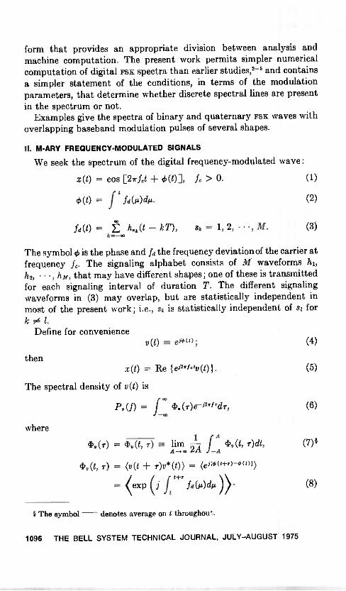
form that provides an appropriate division between analysis andmachine computation. The present work permits simpler numericalcomputation of digital FSK spectra than earlier studies,2-b and containsa simpler statement of the conditions, in terms of the modulationparameters, that determine whether discrete spectral lines are presentin the spectrum or not.
Examples give the spectra of binary and quaternary FSK waves withoverlapping baseband modulation pulses of several shapes.
II. M-ARY FREQUENCY -MODULATED SIGNALS
We seek the spectrum of the digital frequency -modulated wave :
x(t) = cos Prfct + 0(01 > 0.
= f fa(04.
fa(t) = /10 - kT), sk = 1, 2, , M.
The symbol cp is the phase and fd the frequency deviation of the carrier atfrequency L. The signaling alphabet consists of M waveforms h1,h2, , hM, that may have different shapes ; one of these is transmittedfor each signaling interval of duration T. The different signalingwaveforms in (3) may overlap, but are statistically independent inmost of the present work; i.e., sk is statistically independent of 3/ fork 1.
Define for conveniencev(t) = ego;
thenx(t) = Re eflr ce7)(0) .
The spectral density of v(t) is
(D = 43.(7)e-oirirdr,
where
43(r) = (1),,(t, r) fA
cl). (t, r)dt,
43(t, r) = (v(t r)v* (0) = (elice+7)-4'()1)
= (exp (j f t+7 fd(µ)dih ))
§ The symbol - denotes average on t throughout..
1096 THE BELL SYSTEM TECHNICAL JOURNAL, JULY-AUGUST 1975

An arbitrary constant of integration is implicit in the notation of(2), which defines the phase. This is of little consequence in the re-mainder of the present paper, since most of our study is directed to-ward the spectrum of the complex wave v(t); as seen by the final lineof (8), the absolute phase is irrelevant in determining Py(f). Theabsolute phase must be rendered explicit only for the following threepurposes in the present work :
(i) Relating P, (f) to P,,(f) (the spectra of the real FSK wave x(t)of (1) and of the complex FSK wave of (4), respectively).
(ii) Separating possible line -frequency components from the FSKwave.
(iii) Specializing the present FSK treatment to the prior PSK results.'
To make the absolute phase explicit, we writet
95(t) =f
fd (AMA + ; v(0) = (°). (9)
The term 4,(0) is the phase of the FSK wave at t = 0. We consider threerepresentative assumptions for 4)(0) :
(i) 4)(0) deterministic, e.g. :4)(0) = 0. (10)
(ii) OM random, uniform, and independent of the modulation 8k:
d4)Pr [4) < 4)(0) (t) c/4)] = -271- 0 <2r. (11)
4)(0) dependent only on the modulation parameters (or signal-ing pulses) that contribute to fd(0+)§ in (3) :
-kT= hsk(odA. (12)§
k:h.k(-kr+)0 -0.
The signal -pulse duration is assumed finite; consequently, in(12), the E has a finite number of terms, and the lower limiton the f becomes finite. Specific examples of (12) appear inSection IV below. In other words, the net phase contributed byall past signaling pulses that are over by t = 0, i.e., for which1i.k(-01+) = 0,§ is normalized to 0.
The +'s indicate that Id and h,k are to be evaluated an infinitesimal time laterthan 0 and -kT, respectively, if any of the signal pulses have discontinuities at theirupper limits at a time -slot boundary (see Section IV). If the signal pulses and, hence,the instantaneous frequency deviation fd(t) are continuous, these two -F's may bedropped.
SIGNAL POWER SPECTRUM 1097

In the appendix we show that, except for special modulations withlow carrier frequencies fc that take on special values, the followingsimple relation gives the spectrum of the real wave x(t) of (1) :
P.M = I P.Cf - 13.(- f - fc). (13)i
The first term of (13) is the spectrum of the complex baseband wavev(t) shifted to the carrier frequency -1-j; ; the second term is the spec-trum of v*(t) shifted to - fc. More specifically, (13) is valid if any of
the following are true :
(i) Eq. (11) holds, independently of any other considerations.(ii) Eq. (10) or (12) holds, and 1),(f) [and hence Pr(f)] has no
line components.(iii) Eq. (10) or (12) holds, P (f) [and hence P.(f)] has (equally
spaced) line components, and fc is low enough so that the twoterms of (13) overlap, but L is such that the line componentsof the two terms of (13) do not coincide. The discrete valuesforbidden to f, under these conditions are given by (146) inthe appendix.
(iv) The carrier frequency is so large that the two terms of (13) donot significantly overlap, independently of any otherconsiderations.
Consequently, we study only 13,,(f) throughout the remainder of thispaper. This suffices for all cases except that of a low carrier frequencyL that takes on special discrete values related to the baud rate 1/Tand the modulation, for very special modulations that result in line -spectral components (Psi( is one such case, but there are others).
The condition expressed by (12) is assumed in much of what follows.This results in no significant loss in generality in treating the spectrumof the real wave x(t), as discussed above. It permits economy of nota-tion in the general case, a convenient treatment of line componentspresent in special cases, and simple specialization of the present FSKresults to prior PSK results.'
III. NOTATION AND STATISTICAL MODEL
We introduce the vector -matrix notation of the prior PSK study.'Since that study allowed correlated modulation parameters sk while thepresent work is largely restricted to independent sk, only a portion of
Section III of Ref. 1 need be summarized here.
I Compare (5) of Ref. 1.
1098 THE BELL SYSTEM TECHNICAL JOURNAL, JULY-AUGUST 1975
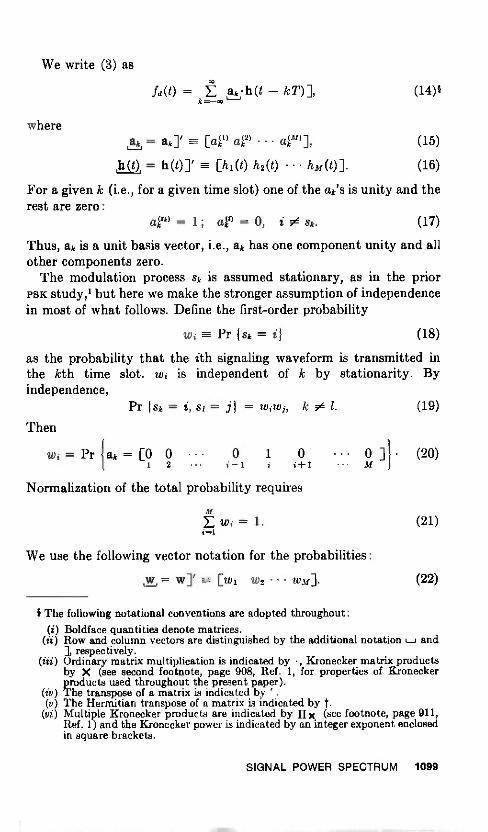
We write (3) as
where
fd(t) = akh(t - kT)],
ak = ak]' [a,1" ae) aiM)],
h(t) = h(t)T = [h 1(t)h2(t) hm(t)].
For a given k (i.e., for a given time slot) one of the ak's is unity and therest are zero :
a (sk) - 1 ctii) = 0, i sk.-k (17)
Thus, ak is a unit basis vector, i.e., ak has one component unity and allother components zero.
The modulation process sk is assumed stationary, as in the priorPSK study,' but here we make the stronger assumption of independencein most of what follows. Define the first -order probability
wi Pr { Sk = i} (18)
as the probability that the ith signaling waveform is transmitted inthe kth time slot. wi is independent of k by stationarity. Byindependence,
Pr sk = i, si = j} = wiwi, k 1. (19)
Then
wi = Pr jak = [0 0 0 1 0 0 ] (20)1 2 i-1 i i+1
Normalization of the total probability requires
ht
E wi = 1. (21)
We use the following vector notation for the probabilities :
w = w, wm]. (22)
I The following notational conventions are adopted throughout:(i) Boldface quantities denote matrices.
(ii) Row and column vectors are distinguished by the additional notation L_1 and], respectively.
(iii) Ordinary matrix multiplication is indicated by ' Kronecker matrix productsby X (see second footnote, page 908, Ref. 1, for properties of Kroneckerproducts used throughout the present paper).
(iv) The transpose of a matrix is indicated by ' .
(v) The Hermitian transpose of a matrix is indicated by t.(vi) Multiple Kronecker products are indicated by 11 x (see footnote, page 911,
Ref. 1) and the Kronecker power is indicated by an integer exponent enclosedin square brackets.
SIGNAL POWER SPECTRUM 1099

Further define a vector (here of dimension M) with all elements unityas
1 = 13' -... [1 1 1].
Then (21) may be written
1w] = w 1] = 1.
Finally, for convenience later, define the diagonal matrix
Wd -=-=
_w1 0
w2
(23)
(24)
(25)
Then, from (22) and (23),
Wd 1] = w], LL-wd = ,2y, (26)
Note that(ak) = w,
(ad ak) = Wd.
(27)
(28)
IV. FSK AS A BASEBAND PULSE TRAIN
We seek an expression of v(t), given by (4), (9), (12), and (14), of
the form
v(t) = i ckr(t - kT)] (29)k--,-.3
for signaling pulses of finite duration. Assume the hi(t) of (3) arestrictly time -limited to an interval KT, as follows :
h(t)] = 0], t 5 LK, t > UK. (30)4
UK ----'
T, K even.
K 1
2T' K odd.
LK E----
2 T'K even.
(31)K ± 1
T, K odd.2
LK and UK are respectively the lower and upper limits of the pulses.Figure 1 shows portions of fd(t) for four different maximum signal -pulse durations; the terms k = -1, 0, 1, 2 of (14) are shown, and for
la, = 0]' is a vector of appropriate dimension (here M) with all elements zero.
1100 THE BELL SYSTEM TECHNICAL JOURNAL, JULY-AUGUST 1975

f, (t),,r\/
/
-1
,
\
U
/
1
/, \/\/ ,z
,,,, . K
////
..I
-1
/ \
.
0
......
1
///
//
2
/' /,x/ \/I N.
\Ni.
K
,/.... ./#
//
-1..... ..._
0
% //i(do ..........
1
........0 ...
///
2
..... "--..N,
\ ....
NN. K
.. .....
.. .../-1
, .......... ....
0 1
...... ..".4%....
_ ... ,
2
-,... .,.....".......>CI ...
"4. .... ...,
,...
K
'''',.. t
-T 0 T 2T 3T 4T
=1
=2
=3
=4
Fig. 1-Frequency modulation for different signal pulse durations. Index k isshown near peak of each pulse. Also, for simplicity, same signal pulse is shown foreach k. T = time slot duration or signaling period. KT = maximum signal -pulseduration. Note different pulse center location for odd and even K.
convenience ak has been taken the same for each of these time slots.The pulses are positioned along the time slots such that the limits ofeach signal pulse lie on the boundary between adjacent time slots (i.e.,t = integer T) ; this results in different definitions for LK, UK for Keven and odd. Since symmetric pulses have been chosen for illustrationin Fig. 1, their maxima are centered in the time slots for K odd, andlie on the time -slot boundaries for K even. Discontinuities are permittedat the pulse edges (and elsewhere), but are not present in the exampleof Fig. 1 (and would not normally be present in a mathematical modelof a physical system) ; discontinuities at the time -slot boundaries arerestricted by the inequalities at the right of (30). Examine the (0, T]
SIGNAL POWER SPECTRUM 1101

time slot in Fig. 1 as typical; then the number of pulses contributingto fd(t) at every instant equals K.§
It remains for us to express the pulse shapes r(t) and coefficients ckof (29) in terms of the signal pulses h(t) and coefficients ak of (14). Wegive separate treatments for the cases K = 1 and K = 2, and extendthese results to general K. The treatment is an extension of that forthe PSK case, given in Section IV of Reference 1.
4.1 Nonoverlapping pulses: K = 1
The top portion of Fig. 1 shows digital frequency modulation forwhich the signal pulses in different time slots never overlap; in thiscase from (30) to (31),
Defineh(t)] = 0], t < 0, t > T.
[exP (j f hi(OdA) exp (j fo' h2(04)
(32)
exp (j f lim0.44)] 0 < t < T.
q ( (33)
L.(2,t<0, t > T.
Equations (4), (9), (12), (14), and (33) yield
0(0) = 0; v(0) = 1. (34)
where
V(t) = Skak"Ct knik=-.3
(35)
0
I ai_iq*(T)], k < 0.i=k+1
Sk 1, k = 0.k
(36)
II ai_Iq(T)], k > 0.i=1
Comparing (35) and (29), the parameters of the latter are given asfollows for nonoverlapping signal pulses:
ck= Sk,122, bk = k;K = 1. (37)
r(t)] = q(t)];
Sk in (37) is, of course, given by (36).
§ The same conventions were used in Fig. 1, Ref. 1, for the baseband modulationpulses in digital PSK.
1102 THE BELL SYSTEM TECHNICAL JOURNAL, JULY-AUGUST 1975
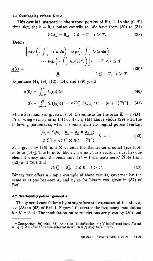
4.2 Overlapping pulses: K = 2
This case is illustrated in the second portion of Fig. 1. In the (0, 71]time slot, the k = 0, 1 pulses contribute. We have from (30) to (31)
h(t)] = 0], t -T, t > T.
Define
[exp (j f TM(E)dµ)/ exp (j f h2(12)d/.1)
exp( j f hm(A)di2)] -T <t-T
q(t) =0 t -T,
Equations (4), (9), (12), (14), and (39) yield0
4)(0) = 118,(A)611L.-T
v(t) = Skfakq(t - kT)]} fak+iq(t - (k
(38)
T.
t > T.(39)§
(40)
1)T)]1, (41)
where Sk remains as given in (36), the same as for the prior K = 1 case.Proceeding exactly as in (51) of Ref. 1, (41) above yields (29) with thefollowing parameters, when no more than two signal pulses overlap :
Ck = Skbk, bk ak X ak+i ;K = 2. (42)
r(t)] = q(t)] X q(t - T)];Sk is given by (36), and X denotes the Kronecker product [see foot-note to (14)]. The term bk, like ak, is a unit basis vector, i.e., it has oneelement unity and the remaining M2 - 1 elements zero.' Note from(42) and (39) that
r(t)] = 0], I < 0, t > T. (43)
Binary FSK offers a simple example of these results, governed by thesame relations between ak and bk as for binary PSK given in (57) ofRef. 1.
4.3 Overlapping pulses: general K
The general case follows by straightforward extension of the above;see (58) to (62) of Ref. 1. Figure 1 illustrates the frequency modulationfor K = 3, 4. The modulation pulse restrictions are given by (30) and
§ Comparing (39) with (33), note that the definition of q(t) is different for differentK; q(t) 0 over the same interval in which h(t) may be nonzero.
SIGNAL POWER SPECTRUM 1103
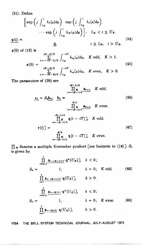
(31). Define
[eXPILK
h1GOCII.4) exp fLx h2(1.04)
q(t)
OM of (12) is
0(0) =
eXP fthM(A)C11-1)]) LK < 1 S UK.LK
(44)t S LK, t > UK.
(K-3)/2 r -kTitak(A)di.L, K odd, K > 1.
k. -(K-1)/2 J LK
(K-2)/2 i-kTlisk(04, K even, K > 0.
- (K-2)/2 J LK
The parameters of (29) are
Ck Skbk; bk
(K-i)/2x K odd.
i- (K-1)12
K/2
II x palt+i, K even.i--(K-2)/2
(45)
(46)
(K-ii/2q(t - iT)), K odd.
i--(K-1)/2
r(t)] = (47)K/2llx q(t - iT)], K even.
i--(K-2) /2
llx denotes a multiple Kronecker product [see footnote to (14)]. Skis given by
0
iiii._(K4.1)/ q*( UK)" k < 0;i-k+1
Sk = 1, k = 0; K odd.
11 ai-(/C+1)/2, q(UK)], k > 0.
0
H ai-(K/2) q* (UK)), k < ;
Sk = 1,
k
11 a i- (Ki 2 )q(U 101i=1
(48)
k = 0; K even. (49)
k > 0.
1104 THE BELL SYSTEM TECHNICAL JOURNAL, JULY -AUGUST 1975

Note thatr(t)] = 0], t < 0, t > T. (50)
4.4 Discussion
It is instructive to obtain the prior PSK results' by specializing thepresent FSK results. Define the phase shift produced by each signalingpulse as
gi(t) = j" hi(A)dA, i = 1, 2, , M (51)LK
g (t)] = fLK
h(A)Jdi.i, (52)
and substitute into (44)* (or into (33) or (39) for special cases K = 1,2). Then the present results of (29), (31), and Section 4.3 are similar tothe former PSK results of (43) and Section 4.3 of Ref. 1, except for thefactor Sk; in particular, the equations for q(t), bk, and r(t) have anidentical form. The additional factor Sk present in the FSK case ac-counts for the total phase shift introduced by each of the signalingpulses.
To specialize the present FSK results to the PSK case, we require thetotal area of each of the present modulation pulses to be zero. Thus,(51) and (52) become
or in vector notation
or
UKMILK) EF- hi(t)dt = 0, i = 1, 2, , M (53)*
J LK
UK
g ( UK) j fLK h(t)]dt = 0].
Substituting in (44),
Therefore, (17) yieldsq(UK)] = 1].
acq(UK)] = 1.
Substituting in (48) to (49),
Sk = 1, all k, K,
(54)ii
(55)
(56)
(57)
completing the specialization of the present FSK results to the PSKcase.'
In the general MK case, the results of Sections 4.1 to 4.3 above reducethe FSK problem to determining the spectrum of (29). This is ac -
Only the range Lk < t 6 Uk is relevant in (51), (52), since q(t) m 0 outside thisrange.
If Equations (30) to (31) and (53), (54) render (51) and (52) zero fort 5 Lic,t z UK, satisfying (58) of Ref. 1.
SIGNAL POWER SPECTRUM 1105
complished by deleting (149), (153), and (163) to (171) of Ref. 1,Appendix B.§ Then the spectral density of (29) above is given by settingb -> c in (150) to (152) and (160) to (162) of Ref. 1 as follows:
1'v(f) = R(i) -I). (iT) R*(ni. (58)
...
P.m = f e-"ilne.(n) (59)§§n= --co
C(n) = (ck+.1c;) (60)
R(f)] = R(f)' = f ce e-iwtr(t)]dt. (61)
In these relations R(f) is the Fourier transform of r(t) of (37), (42), or(47), depending on K (i.e., the amount of pulse overlap). tic(n) is de-termined from (36) and (37), (36) and (42), or (46) and (48) or (49)in Section VI for K = 1, 2, and general K, respectively.
V. FSK WITH LINE COMPONENTS
From (21), (22), and (44),
lwq(Ux)1 --.. 1. (62)§§§
We show in the present section that equality in (62) corresponds tothe presence of line components in the FSK spectrum. Conversely, ifthe inequality of (62) is satisfied, we see in Section VI that the FSKspectrum contains no line components.
Assume throughout the remainder of the present section that
lwq(Ux)] i = 1. (63)
This yields
LK
where 2rfi is defined as the common area (mod 2r) of all of the FSKsignaling pulses in the line case. For definiteness we take
UK
Equivalently,
hi(t)dt = 27fi + integer 27, i = 1, 2, , M, (64)
-1 < h 1. (65)
q(UK)] = Orli 1], -1 < fi ' 1. (66)
i These deleted portions were relevant to the study of line spectral components ofPSK.1 The line spectral components of FSK are treated separately in Section V.
i§ See footnote, page 905, Ref. 1.Hi This follows because I qi(01 = 1.
1106 THE BELL SYSTEM TECHNICAL JOURNAL, JULY-AUGUST 1975
Now substitute (66) into (48) and (49) ; we haveSk = ejk2rf
Thus, when (62) is satisfied
all k, K. (67)
V (t) = eik2'i bk r (t kT) J.k=-.
(68)
The relation (68) is the same as the PSK result of (43) of Ref. 1except for the factor eik2Tf 1 ; as noted following (52), bk and r(t) havethe same form in FSK and PSK. Consequently, when (63) is satisfied, theFSK spectrum may be obtained by simple transformation of the PSKresults of Ref. 1. One way this may be done is to rewrite (68) as
v(t)e-.12.(111T)t (e-j2.(flIT)(t-knr(t - kT)]). (69)
Comparing with (43) of Ref. 1, all the PSK results of Ref. 1 applydirectly to the present case by making the substitutions
v(t) v(t)e-i27(filT)t,r(t)] e-12ircnint r(t)].
Therefore, when (68) is satisfied, and consequently (68) holds, theFSK wave has line spectra. We separate the line and continuous com-ponents as
v(t) = + Mt). (71)
The line component is given from (70), and (114)§ of Ref. 1, as
vi(t) = -1- w[K] E RT n
(n + ft)] 02.«.-Ffoi7')t,
(72)§§
Pvt(f) = 71-72 R(Di12 5 (f n fl)n= -
The spectral density of the continuous component is found from (70),and (69),§§§ (96), or (116) of Ref. 1 as follows :
Pvc(f) = -T R(f) R* (f) i
(70)
(73)
Or from (66) and (95) of Ref. 1 for the special cases k = 1, 2.§§ See footnote to (14); an exponent enclosed in square brackets denotes the
Kronecker power, i.e., the Kronecker product of a matrix (or vector) with itself theindicated number of times.
§§§ This is equation (69) of Ref. 1 specialized to independent signal pulses, i.e.,with (32) used for all n 0, yielding (72) or (73), of Ref. 1. If this restriction is notimposed, and (70) above is used in the general form of (69) of Ref. 1, we obtain thespectrum of digital FSK with line spectra, with nonoverlapping signal pulses havingarbitrary correlation (rather than being independent, as in the remainder of thepresent paper). This is the only correlated case that can be readily treated by thepresent methods.
SIGNAL POWER SPECTRUM 1107
= via - w].w, K=1. (74)
wp] w][2] .NAT [2]
(W X Wd X w] w] [2] w [2] )e-j2w(fT-f1)
+ (w] X Wd X w w3[2].w[21)e-Fi2/T-ft), K = 2. (75)§
expression in { in (116) ofRef. 1 with fT fT -
The condition of (63), that has here been shown sufficient, is shownin Section VI also to be necessary for line components to be presentin FSK spectra. This condition has a simple physical interpretation.Every signal pulse must introduce the same total phase change in themodulated carrier in order to have line components. This phase changehas been denoted as 211/ ; the line components appear at frequencies
(fcn
T
general K. (76)
(77)
When ft = 0, (73) to (76) show that the FSK spectra are identical tothe prior PSK results.' However the wave in this case is not necessarilya PSK wave. The stronger condition of (53) or (54) is required to havea PSK wave; this condition demands the net phase shift introduced byevery signaling pulse to be zero. A wave with ft = 0, but one or moresignal pulses with net phase change equal, for example, to 27r, willhave a spectrum given by the PSK formula, but will not be a PSK wave.
VI. FSK WITH NO LINE COMPONENTS
Assume throughout this section that the inequality of (62) is
satisfied :1,2S. (Ux):1 < 1. (78)
We demonstrate that under these conditions the FSK spectrum containsno lines. The properties of Kronecker products given in Ref. 1 in thesecond footnote, p. 908, and in the first footnote, p. 915, are usedthroughout without further comment.
6.1 FSK spectrum with no line components: nonoveriapping pulses, K =
From (37) and (60),
*.(n) = ((Sk+.4)(ak+.]ak)). (79)
From (36),n-1
Sic+ nSk = E ak+iq(T)3, n. > 0. (80)i-o
§ See footnote to eq. (72).
1108 THE BELL SYSTEM TECHNICAL JOURNAL, JULY-AUGUST 1975
Let us first consider C(0). Since SkS: = 18k 12 = 1, for all k, wehave from (79) and (28)
4;.(0) = wd (81)
Next, (79) and (80) yield
4),(n) = 111.11ak+iq(T)]} fq(T)ak]}{ak+.1akl, n >= 1, (82)
where we have split off the first factor of (80). For n = 1, the first{ } , containing the II, is dropped. The first { } is independent of theremainder of the expression by (19); using the fact that q(71) ak] is acomplex number or equivalently a 1 X 1 complex matrix, and using(27) and (28),
cic(n) = fmq(T)]In-i(ak±n}q(T)akIE)= 1E2q(T)]In-Ifw]q(T).wd), n __>=- 1, (83)
the last step following from the independence of ak+n and ak.Finally, taking the Hermitian transpose§ of (79),
iiot (n) = ( (4+ nSk) (ak] ak+ n) ). (84)
Alternatively, setting n -> -n in (79),
oc( -n) = ((g;Sk_n)(ak,]12.,J, >. (85)
Since (79) has been shown independent of k, we may set k -+ k + nin (85), to yield upon comparison with (84)
tic ( - n) = (14 (n). (86)
From (58) to (61), (81), (83), and (86),
Pc(fT) = A + At,
A = lwd + e-.7.2.../Twi.g(T).wd f {e-j2rfT w.cni) n-1.n....1
Because of (78) the geometric series in (88) converges, and
1e-j2rfT wl.q(T)
A =2-
wd + 1 - e-j2T1T wq(T)].
.w,"
Finally, the spectrum of the complex FSK wave of (4) is
1P(f) =T-
R(f) (A + At) R*(f)),
with A given by (89) for nonoverlapping pulses, K = 1.
§ See footnote to (14).
(87)
(88)
(89)
(90)
SIGNAL POWER SPECTRUM 1109
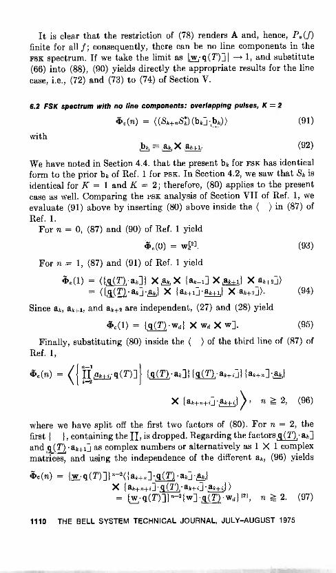
It is clear that the restriction of (78) renders A and, hence, Pv(f)finite for all f; consequently, there can be no line components in theFSK spectrum. If we take the limit as I wq(T)] I -> 1, and substitute(66) into (88), (90) yields directly the appropriate results for the linecase, i.e., (72) and (73) to (74) of Section V.
6.2 FSK spectrum with no line components: overlapping pulses, K = 2
(lc (n) = ((Sk±ngD(bk111-O) (91)
withbk --- ak X ak+1. (92)
We have noted in Section 4.4. that the present bk for FSK has identicalform to the prior bk of Ref. 1 for PSK. In Section 4.2, we saw that Sk isidentical for K = 1 and K = 2; therefore, (80) applies to the presentcase as well. Comparing the PSK analysis of Section VII of Ref. 1, weevaluate (91) above by inserting (80) above inside the ( ) in (87) ofRef. 1.
For n = 0, (87) and (90) of Ref. 1 yield
$c (0)= wP3. (93)
For n = 1, (87) and (91) of Ref. 1 yield
(13.(1) = (1,01),ak11 X AL, X fak+1] X ,ak+1,) X ak+2])= ({q(T)ak].,L,G) X { ak+dak±i} X ak+2]). (94)
Since ak, ak+1, and ak+2 are independent, (27) and (28) yield
&(1) = {q(T)wd} X wd X w]. (95)
Finally, substituting (80) inside the ( ) of the third line of (87) ofRef. 1,
ec(n) = (012,ak+i,q1(T)1} 1 q(T) ak]H q(T) ak±d} { ak±n].1,Lj
X fak+n+il ' ak-Fil) 1n .?_-__ 2, (96)
where we have split off the first two factors of (80). For n = 2, thefirst { }, containing the fl, is dropped. Regarding the factors q(T) ak]and q(T) ak+i] as complex numbers or alternatively as 1 X 1 complexmatrices, and using the independence of the different ak, (96) yields
4.c(n) = fyirA(T)11n-2(1 ak+n] q(T) ak] AL,}X lak±n±i]q(T) ak+iiak-Fil)= imrq(7)11n-2{wl.q(T),wd) [2], n>_2. (97)
1110 THE BELL SYSTEM TECHNICAL JOURNAL, JULY-AUGUST 1975

The remainder of the analysis proceeds as in Section 6.1. The FSK
spectrum for overlapping pulses with K = 2 is given by
1Pv(f) = -T R(f) (A + At) R*(f)], (98)
where
A 1_ wc2] e-j2rf T 1,-( ) X wd X w]
2 a
e-j2TfTwl ( .wd 1 (2]
1 - e-i2T/Ta iq(T)](99)
Pv(f) again contains no spectral lines by (78) ; the limit I wq(T)] -+ 1again yields the appropriate results of Section V for the line case.
6.3 FSK spectrum with no line components: overlapping pulses, general K
Similar analysis yields the generalization to any overlapping signalpulses. From (46) and (60),
41),(n) = ((Sk+.4)(bk]120) (100)
with bk given by (46) and Sk by (48) to (49). Thus,
jj K + 1ak-((x+1)/2)+;:q
gillk odd,
2
ak-(KI2)+j qK m/ )] k even, (101)
Since the present bk have identical form to bk of Ref. 1, (100) isevaluated by substituting (101) inside the ( ) of (106) of Ref. 1, andmaking corresponding changes in the remainder of Section VII, Ref. 1.The factor
Sic* OS: =
ar q(UK)]
n > 0.
(102)1
is inserted inside the ( ) of (107) of Ref. 1. In the following we recallthat the factors of (102), ,, q] = la], may be regarded alternativelyas complex numbers or as 1 X 1 complex matrices.
In (109) of Ref. 1, the first factor of the second line is modified as
(ai) -> q(UK) (ad ai) = q(U.K)wd; (103)
consequently,4.(1) = fq(UK)wdl X wV-3.1 X w]. (104)
In (110), Ref. 1, the first two factors of the fourth line are modified
§ UK is given by eq. (31).
SIGNAL POWER SPECTRUM 1111
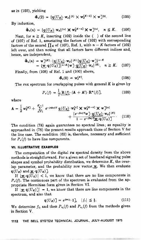
as in (103), yielding
6. (2) = q ( UK) wd} [21 X W[K-2] X w][2]. (105)
By induction,
-6.(n) = q(UK)Wcil (n] X WV -n3 X w] ]n], n s K. (106)
Next, for n > K, inserting (102) inside the ( ) of the second lineof (107) of Ref. 1, associating the factors of (102) with correspondingfactors of the second flx of (107), Ref. 1, with n -K factors of (102)left over, and then noting that all factors have different indices and,hence, are independent,
3c(n) = wi [KJ {A( UK), wd (K] ( UK) wl n-K= 1m. CU ic)i}n-K fw]. ir) w di [IC] n z K. (107)
Finally, from (108) of Ref. 1 and (100) above,
C(0) = wV3. (108)
The FSK spectrum for overlapping pulses with general K is given by
1P, (f) = -T R (f) (A + At) R* (f)],
where
1 K-1A
=WOK]e-1n2717' ( UK) wkl] X wV -n3 X w] ]n]
e-i2T/Tw] q ( UK) wd } EK1
1 - e-fliriTyL q ( UK)]
The condition (78) again guarantees no spectral lines ; as equality isapproached in (78) the present results approach those of Section V forthe line case. The condition (63) is, therefore, necessary and sufficientfor Py(f) to have line components.
(109)
(110)
VII. ILLUSTRATIVE EXAMPLES
The computation of the digital FM spectral density from the abovemethods is straightforward. For a given set of baseband signaling pulseshapes and symbol probability distribution, we determine K, the over-lap parameter, and the probability row vector w We then evaluateq ( UK) and m q ( UK)].
If lay,. q ( UK) I < 1, we know that there are no line components inP,(f). The continuous part of the spectrum is evaluated from the ap-propriate Hermitian form given in Section VI.
If I w q (UK)] I = 1, we know that there are line components in thespectrum, and also that
q(UK)] = Offi 1], l id 5 . (111)
We determine ft, and then P., (f) and P (f) from the methods givenin Section V.
1112 THE BELL SYSTEM TECHNICAL JOURNAL, JULY -AUGUST 1975
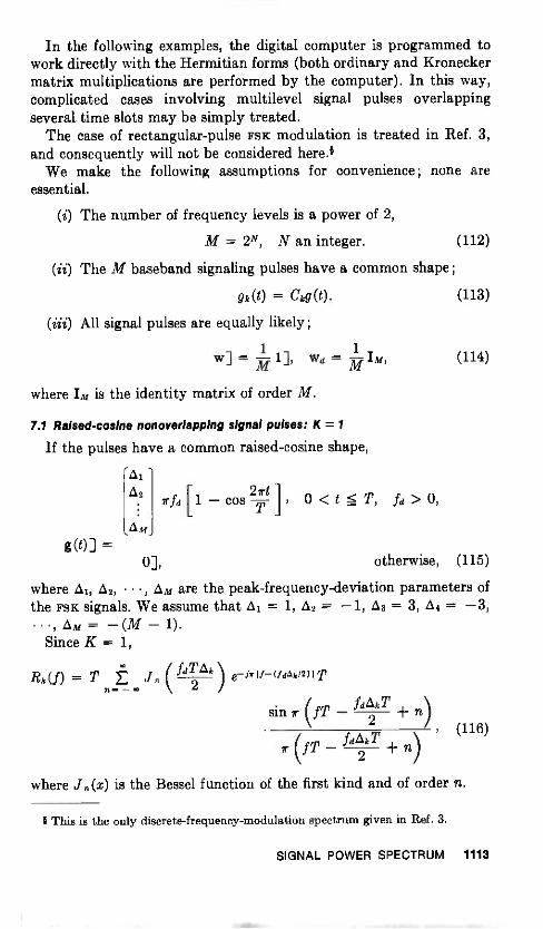
In the following examples, the digital computer is programmed towork directly with the Hermitian forms (both ordinary and Kroneckermatrix multiplications are performed by the computer). In this way,complicated cases involving multilevel signal pulses overlappingseveral time slots may be simply treated.
The case of rectangular -pulse FSK modulation is treated in Ref. 3,and consequently will not be considered here.§
We make the following assumptions for convenience; none areessential.
(i) The number of frequency levels is a power of 2,
M = 2N, N an integer.
(ii) The M baseband signaling pulses have a common shape ;
gk(t) = Ckg(t).
(112)
(113)
(iii) All signal pulses are equally likely ;
1wd = IM,w] = ri 11 m (114)
where IM is the identity matrix of order M.
7.1 Raised -cosine nonoverlapping signal pulses: K =1
If the pulses have
-Al
a common raised -cosine shape,
02 irfd[i - cos 2--2--q],T
0 <t_T, fd> 0,
g(g)] =Am
0], otherwise, (115)
where AI, A2, , AM are the peak -frequency -deviation parameters ofthe FSK signals. We assume that Ai = 1, A2 = -1, As = 3, A4 = -3,
, Am = - (M - 1).Since K = 1,
Rk(i) = T Ejn(fdT
2Ak)- coe-il, If--(idak/2)1T
sin 7 (fT fd A2k T -{-n]
7 (fT f 'it'll + n) '
(116)
where Jn (x) is the Bessel function of the first kind and of order n.
I This is the only discrete -frequency -modulation spectrum given in Ref. 3.
SIGNAL POWER SPECTRUM 1113

7.1.1 Raised -cosine signaling with no line spectrum: K = 1
Sinceq(U1) = e f eiAMTidT, (117)
line spectra are absent if and only if fag' is not an integer. In this case,
1P,(f) = P(f) = -T R (f) (A + At) R (nt,
4
0.5
(0.350)
fdT=0.50
1.0 2.0
(a)
(0.00614)
2.5 3.0
(118)
Fig. 2-Spectral density of binary FSK system with raised -cosine signaling andpulse duration T. K = 1. 2fd is the spacing between two adjacent a priori chosenfrequencies.
1114 THE BELL SYSTEM TECHNICAL JOURNAL, JULY-AUGUST 1975
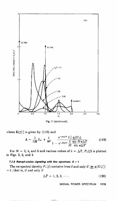
(0.198)
2
0.5
(0.194)
1.0
fdT=1.5
1.75
1.25
1.5
fT
2.00
Fig. 2 (continued).
(b)
A (0.0481)
2.0 2.5 3 0
where R(f)] is given by (116) and
1 1 e-AwfT 1]q(Ui)A =
21,11IIf ±M2 (119)1 sin /ifirfdT1 - e--,r/T
M sin irfdT
For M = 2, 4, and 8 and various values of k = fdT, P. (f) is plottedin Figs. 2, 3, and 4.
7.1.2 RaIsed-cosine signaling with line spectrum: K = 1
The FM spectral density Pv(f) contains lines if and only if Iy_7, q (U1)]=1; that is, if and only if
fdT = 1, 2, 3, . (120)
SIGNAL POWER SPECTRUM 1115

(0.244)
//
0
(0.141)
fdT=0.25
A (0.140)
(a)
(0.0199)
( b)
2.00
fdT=1.25 // 1.55\\ / // 1.75
// //(0.0005)
I I
0 0.5 1.0 1.5 2.0 2.5
fT3.0
Fig. 3-Spectral density of quaternary FSK system with raised -cosine signalingand pulse duration T. K = 1. 2fd is the spacing between two adjacent a priori chosenfrequencies.
1116 THE BELL SYSTEM TECHNICAL JOURNAL, JULY-AUGUST 1975
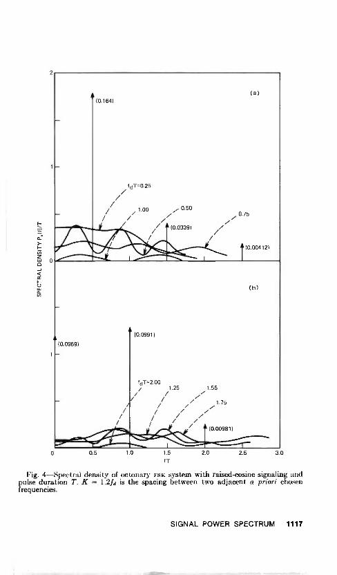
A(0.0969)
1
(0.164)
0.5
fdT=0.25///1.00 0.50
/ /Z/0.75// /// 6 (0.0339) /// /
(0.0991)
1.0
fdT=2.001 1.25 1.55
/ / // /r
// 1.75/ /
/ // / z/
/ //
1.5
fT
2.0
(0.00981)
(a)
1(0.00412)
2.5
b)
3.0
Fig. 4-Spectral density of octonary FSK system with raised -cosine signaling andpulse duration T. K = 1.2fa is the spacing between two adjacent a priori chosenfrequencies.
SIGNAL POWER SPECTRUM 1117

In this case,ft = 1,ft = 0,
(121)
. (122)
fdT = 1,fdT = 2,
3,
4,
5,
6,
,
From Section V,
1/3,,(f)=T-12-M1 R (Di 12 E a r f n ±Tft
n = -1
R(i) (B B1) R(f)t,
1.5
1.0
0.5
0
(0.221)
fdT=0.125
0.250
0.350
0.500
A (9.568X 10- 5)
(1.559X10⁻⁸(
0.5 1.0 1.5 2.0 2.5
f T
(a)
3.0
(123)
Fig. 5-Spectral density of binary F5K system with raised -cosine signaling andpulse duration 2T. K = 2.2f d is the spacing between two adjacent a priori chosenfrequencies.
1118 THE BELL SYSTEM TECHNICAL JOURNAL, JULY-AUGUST 1975
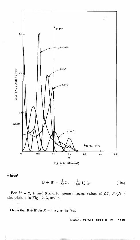
1.5
0.5
(0.0125)
where§
(0.182)
fdr- 0.625
0.750
_-0.875
(2.88X10⁻⁴)
2 0 2.5
Fig. 5 (continued).
1 1B + Bt = - I if 11.131 1112
(b)
3.0
(124)
For /II = 2, 4, and 8 and for some integral values of fdT, Pv(f) isalso plotted in Figs. 2, 3, and 4.
§ Note that B Bt for K = 1 is given in (74).
SIGNAL POWER SPECTRUM 1119

2.0
1.5
1.0 -
0.5
r fdT=0.125
(2.673X10⁻²)
0.250
/7
0.500
(4.064X10⁻²)
0.375
(1.192X10⁻⁴)
(a)
0.5 1.0 15
fT
2.0 2 5 3.0
Fig. 6-Spectral density of quaternary FSK system with raised -cosine signalingand pulse duration 2T. K = 2.2fd is the spacing between two adjacent a priorichosen frequencies.
1120 THE BELL SYSTEM TECHNICAL JOURNAL, JULY-AUGUST 1975

1.0
a(3.206X10⁻²)
0.750
0.5 - fdT=0.625
(2.87X10⁻²)
(b)
1.000
4,1%4 A
/ A
// (1.98X10⁻²)// 0.875
0 0.5 1.0 1.5
f T
Fig. 6 (continued).
2.0 2.5
7.2 Raised cosine overlapping signal pulses: K = 2
If a raised -cosine signal pulse just fills up two time slots,
6,2rfd (1 + cos 1-tLT) < t 71,
Am
g(t)] =
Id > o
3.0
0], otherwise, (125)
K = 2, and the spectral density may be calculated from Sections 4.2,V, or 6.2 according to whether
la.v._,01(U2)] = 1 (126)
orla_; (-72) I < 1. (127)
If O1= 1, 0.'_ -1, 63 = 3, O4= 3, y
p1-1= (211-1),AM = (Ill - 1), (116) can be shown to be satisfied if and only if2fdT is an integer. Further,
I/ = 0,and
= z,
if fdT = 1, 2, 3, ,if fdT = 2, 1, 2,
(128)
(129)
SIGNAL POWER SPECTRUM 1121

In this case, note that1 sin (21117fdT)
1. q(T)1111 sin (2lrfdT)
In this case, the FSK spectrum contains line components, and the con-tinuous and line spectra for 111 = 2 and 4 are shown in Figs. 5 and 6.
If 2fdT is not an integer, the FSK spectrum does not contain any lines,and the continuous spectrum given by (97) to (98) for 111 = 2 and 4is also plotted in Figs. 5 and 6.
Several observations can be made from Figs. 2 to 6. For both K = 1and K = 2, discrete spectral lines appear as fdT approaches the limitingvalue and the power in the lines is substantial for K = 1 and M = 2.Also note that power in the line components with K = 2 is smallerthan the power in the lines with K = 1.
For the same value of fdT and K, the principal portion of the spec-trum of binary FSK is narrower than that of quaternary FSK. For K = 1,quaternary FSK spectrum is narrower than that of octonary FSK spec-trum for the same value of fdT.
Since lines can appear in the spectrum for a set of values of fdT,the FSK spectrum is quite different from the PSK spectrum even whenlines are present in the FSK spectrum.
VIII. SUMMARY AND CONCLUSIONS
(130)
Matrix methods are given to express the spectral density of a carrier,frequency -modulated by a random baseband pulse train, in a conciseand computable form. Arbitrary pulse shapes may be used for M-arydigital signaling, and they may overlap over a finite number of signalintervals.
The spectral density is expressed as a compact Hermitian formsuitable for numerical computation by a digital computer. The com-puter is readily programmed to perform matrix operations directly,rather than expanding the Hermitian form and evaluating the indi-vidual terms. In this way, quite complicated cases involving multilevelsignal pulses overlapping several time slots may be treated simply.
Simple conditions in terms of the modulation parameters are givenunder which discrete spectral lines are present in the spectrum. Amethod is given to evaluate the power in the discrete spectral lines.The utility of the method is illustrated by giving several examples.
The present results are restricted to independent signal pulses,except for the very special case of nonoverlapping (K = 1) signalpulses with line spectra present [see footnote following (72)]. In Ref. 1we saw that for overlapping signal pulses with K = 2 (i.e., signalpulses that occupy no more than two time slots), PSK with correlated
1122 THE BELL SYSTEM TECHNICAL JOURNAL, JULY -AUGUST 1975
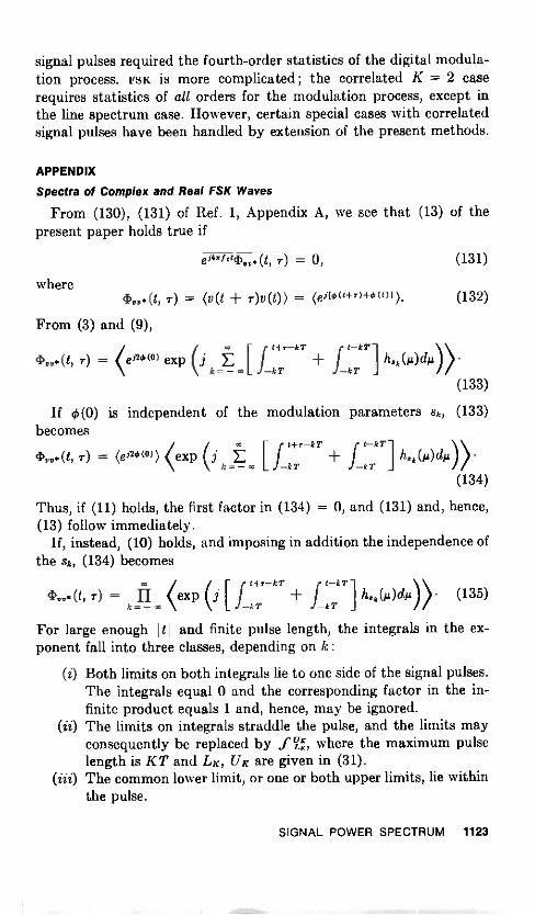
signal pulses required the fourth -order statistics of the digital modula-tion process. FSK is more complicated ; the correlated K = 2 caserequires statistics of all orders for the modulation process, except inthe line spectrum case. However, certain special cases with correlatedsignal pulses have been handled by extension of the present methods.
APPENDIX
Spectra of Complex and Real FSK Waves
From (130), (131) of Ref. 1, Appendix A, we see that (13) of thepresent paper holds true if
eorfac13.(t, r) = 0, (131)
where43.(t, r) = (v(t r)v(t)) = (eaks(g1-7)+0(0)). (132)
From (3) and (9),t-kTt-i-r-kT
]liak(14)4))k=- .1-kr -kT
(133)
If gt, (0) is independent of the modulation parameters sk, (133)becomes
t+r-kT
kT4),*(t, T) = (02")) (exp (j E
k= - L
(134)
Thus, if (11) holds, the first factor in (134) = 0, and (131) and, hence,(13) follow immediately.
If, instead, (10) holds, and imposing in addition the independence ofthe sk, (134) becomes
ao r f t+r-kTCva(t, r) = II( J-
exp (j - /4,044)). (135)k=- L kr kr
For large enough I tl and finite pulse length, the integrals in the ex-ponent fall into three classes, depending on k:
(i) Both limits on both integrals lie to one side of the signal pulses.The integrals equal 0 and the corresponding factor in the in-finite product equals 1 and, hence, may be ignored.
(ii) The limits on integrals straddle the pulse, and the limits mayconsequently be replaced by fa, where the maximum pulselength is KT and LK, UK are given in (31).
(iii) The common lower limit, or one or both upper limits, lie withinthe pulse.
SIGNAL POWER SPECTRUM 1123
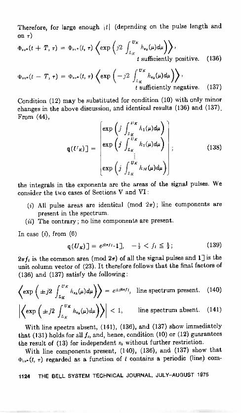
Therefore, for large enough I ti (depending on the pulse length andon r)
UK
CD *(t T, 7) = (13* (t, r) (exp (j2L
14,(1)4)) Kt sufficiently positive. (136)
UK
,,.(t - T, r) = 7-) (exp -j2 f h.,(µ)4)),LK
t sufficiently negative. (137)
Condition (12) may be substituted for condition (10) with only minorchanges in the above discussion, and identical results (136) and (137).From (44),
q( UK)] =
K
UKexp hi(A)dii)
LUK
exp h2(12)41)LK
UK
J h MOAN!)exp (j
(138)
the integrals in the exponents are the areas of the signal pulses. Weconsider the two cases of Sections V and VI :
(i) All pulse areas are identical (mod 2r) ; line components arepresent in the spectrum.
(ii) The contrary ; no line components are present.
In case (i), from (6)
q(UK)] = ei2T/111, < fi S I; (139)
27rfi is the common area (mod 2r) of all the signal pulses and 1] is theunit column vector of (23). It therefore follows that the final factors of
(136) and (137) satisfy the following :
(exp j2 fLKUK h8k(u)dm)) = e±'4.1`, line spectrum present. (140)
(exp (± j2 fLuKK h.k(A)diA)) < 1, line spectrum absent. (141)
With line spectra absent, (141), (136), and (137) show immediatelythat (131) holds for all f,, and, hence, condition (10) or (12) guaranteesthe result of (13) for independent sk without further restriction.
With line components present, (140), (136), and (137) show that7-) regarded as a function of t contains a periodic (line) corn -
1124 THE BELL SYSTEM TECHNICAL JOURNAL, JULY -AUGUST 1975

ponent. Therefore, we write
43.(t, r) = c13. (t, r)/ (1)-.(1, T)c, (142)
where
and4).* (t, 7). = 0, I t I sufficiently large, (143)
4)vv*(t, = ej4.1.1(tIT) cOn(T)ei"2.(e1T).n = -oce
(144)1
Only the line component (144) can possibly contribute to the averageon the left-hand side of (131) :
eorfac13.(t, T)r) lirn1 A ej2r[2.1,1-(2. i+n)I T1 tdt
n = - A-.. 2A -Asin 27[2b (2fi n)/TJA
27[2b (2fi n)/T]A (145co(r) iim)The lim 0 if 2b (2f1 n)/T X 0 for every integer n, thussatisfying (131). Hence, condition (10) or (12) and
2 ( IT; ) X Tn, it. = 0, 1, 2, 3, , (146)
guarantees the result of (13) for independent sk. Since, by (72), the linespectral components of v(t) occur at (ft n)/T, (146) is equivalent torequiring that the line components of v(t)el2rict and of v*(t)e-j2i1.'never coincide. Note that condition (5) of Ref. 1 is the special case of(146) above for ft = 0.
Finally, (135) to (140) of Ref. 1, Appendix A apply also in the presentcase, and establish that (13) is a good approximation if fc is high enoughso that there is no significant overlap between the two terms of (13).
REFERENCES
1. V. K. Prabhu and H. E. Rowe, "Spectra of Digital PM by Matrix Methods,"B.S.T.J., 53, No. 5 (May -June 1974), pp. 899-935.
2. W. R. Bennett and S. 0. Rice, "Spectral Density and Autocorrelation FunctionsAssociated with Binary Frequency Shift Keying," B.S.T.J., 42, No. 5 (Septem-ber 1963), pp. 2355-238.3.
3. R. R. Anderson and J. Salz, "Spectra of Digital FM," B.S.T.J., 44, No. 6 (July -August 1965), pp. 1165-1189.
4. J. E. Mazo and J. Salz, "Spectra of Frequency Modulation with Random Wave-forms," Information and Control, 9, No. 4 (August 1966), pp. 414-422.
5. 0. Shimbo, "General Formula for Power Spectra of Digital FM Signals," Proc.IEE (GB), 113, No. 11 (November 1966), pp. 1783-1789.
6. F. A. Graybill, Introduction to Matrices with Applications in Statistics, Belmont,Calif.: Wadsworth, 1969, Section 8.8.
7. D. E. Cartier, "The Power Spectrum of PCM/FSK-AM/PM," IEEE Trans. onComm., (70M-21, No. 7 (July 1973), pp. 847-850.
'These (PH are generalizations of those in (133) of Ref. 1, Appendix A.
SIGNAL POWER SPECTRUM 1125

11Mt MERIAE,t ,1,1*
Copyright © 1975 American Telephone and Telegraph CompanyTHE BELL SYSTEM TECHNICAL JOURNAL
Vol. 54, No. 6, July-August 1975Printed in U.S.A.
Analysis of Trunk Groups Containing Short -Holding -Time Trunks
By L. J. FORYS and E. J. MESSERLI(Manuscript received July 1, 1974)
This paper presents models for the behavior of trunk groups containingshort -holding -time faulty trunks. The models, referred to as ordered selec-tion, two-sided selection, random selection, or queuing selection, areapplicable to selection procedures used by a number of switching systems.Each model is analyzed to obtain the fraction of group attempts carriedon a faulty trunk in the group, and the corresponding fraction of groupattempts that find all trunks busy (blocking or overflow). Numericalresults for the basic models are also presented. The results indicate thatfactors such as the trunk selection procedure or the type of group (highusage or final) can lead to significant differences in the performance of agroup containing a faulty trunk.
I. INTRODUCTION
A message trunk, the basic connecting link in the switched telephonenetwork, provides the supervising, signaling, and ringing capabilitiesessential to call set-up, as well as the communication path. When acondition that prevents proper functioning of a message trunk occurs,and causes a call failure, the trunk is normally released by a switchingsystem on customer abandonment of the failed attempt and is thenavailable to fail another call. As a result, a single undetected faultytrunk can fail a disproportionate fraction of the offered attempts to agroup. Figure 9 shows an illustrative case where one trunk, subse-quently verified to have been faulty, carried 35 out of 77 attemptsoffered to a trunk group during one hour. Because of their potentialservice impact, such trunks are of major concern throughout the BellSystem and the object of many preventive maintenance and troubledetection programs.
This paper presents models and analyses for the behavior of trunkgroups containing short -holding -time trunks. This terminology is usedto emphasize that the faulty trunks of interest are accessible by thecustomer, as opposed to faulty trunks that inhibit seizure by aswitching system (false busys) or that result in an automatic retrial on
1127
another trunk when an abnormal condition is detected. The modelswere developed to provide tools for quantifying the potential impactof short -holding -time trunks, to help determine more effective waysto use the trouble detection resources in the network. Although themain emphasis here is on the analytical development of the models,some numerical results are also presented. The reader primarilyinterested in these results can refer directly to Section III. (Necessaryterminology and the relationship of the idealized models to switchingsystems are summarized in Section 2.1 and Table I, respectively.)A more detailed outline follows.
The basic models studied, referred to as ordered selection, two-sidedselection, random selection, and queuing selection, and the switchingsystems to which they primarily apply, are summarized in Table I.Justification for the choice of the models is given in Ref. 1. Basicassumptions are Poisson input, exponential holding times for bothnormal- and short -holding -time trunks,* and no retrials because ofblocked or ineffective attempts.t Within this framework, the impactof a short -holding -time trunk depends on its position in the group andon the way idle trunks are selected. Impact is quantified in terms of thefraction ineffective (fraction of offered attempts carried on the short -holding -time trunk) and the blocking (fraction of offered attempts thatfind all trunks busy in the group). These measures enable total ineffec-tives for both high usage groups (fraction ineffective) and final groups(fraction ineffective plus blocking) to be determined, as well as permitthe distortion in standard traffic measurements (group usage andcounts of offered and overflow attempts) owing to a short -holding -time trunk to be assessed. It should be noted that blocking, used herein a conventional traffic engineering sense, is used by some to referto call failures resulting from any cause.
In Section II, prior work is briefly discussed and analysis for thevarious models is developed. Terminology common to the models issummarized in Section 2.1. In Section 2.2, ordered selection is con-sidered. An exact solution for the fraction ineffective is obtained. Thecomputations for the special case of one short -holding -time trunk aresummarized in (14) to (18). Blocking is treated in an approximate way,using the equivalent random method.'
For two-sided selection (Section 2.3), the fraction ineffective isapproximated by using results for ordered selection. The computa-
Although our main interest is short -holding -time trunks, some results hold for ashort or long holding time on one trunk. In these cases, the trunk is referred to asabnormal.
t The models, however, can be used with retrials, if these are also treated as Poisson(this approximation was found to be reasonable). However, the inclusion of retrials(which are an important factor in considering volume changes) does not substan-tially change the service impact of a short -holding -time trunk.
1128 THE BELL SYSTEM TECHNICAL JOURNAL, JULY-AUGUST 1975

Table I - Summary of models for machine trunk selection
Trunk SelectionModel Description
Ordered selection
Two-sided selection
Random selection
Queuing selection
Fixed -order hunt for an idletrunk.
Traffic split into two parts. Eachpart uses a fixed -order hunt foran idle trunk, with the twoorders reversed.
Equally likely choice of an idletrunk.
Trunk that has been idle thelongest is chosen.
Switching System*
Step-by-step, Panel, No.4 Crossbar
No. 1 Crossbar, Cross-bar Tandem, No. 4Crossbar (two-way)
No. 5 Crossbar
No. 1 Electronicswitching system
* Groups are assumed one-way (trunks are selected from only one end of thegroup), except for No. 4 Crossbar (two-way), where a two-way group between No. 4Crossbar systems is assumed. The applications are not always precise; trunk assign-ments to frames, gradings, and certain subgrouping arrangements can affect theselection procedure of some systems.
tions summarized in (25) to (37) give good results for the fractionineffective. Blocking is also treated in an approximate way.
Random and queuing selection are considered in Section 2.4. It isshown that, for fraction ineffective and blocking, these are equivalent.Simple exact solutions involving the Erlang B formula are obtained.Equation (60) gives the fraction ineffective, and eq. (61) gives theblocking.
Numerical results are given in Section III. For reasonable valuesof normal- to short -holding -time ratios as suggested by field data(about 5 to 30, depending on the type of fault and type of traffic), theresults confirm that a single short -holding -time trunk can have asevere impact on service. For example, Fig. 6 shows the impact of oneshort -holding -time trunk in a group with random/queuing selection.It is apparent that the short -holding -time trunk has a significantimpact over a wide range of conditions.
For any group, assuming that a short -holding -time trunk is equallylikely to be in any position,* the various disciplines can be compared.We find that (see Fig. 8)
Averagefractionineffectiveforrandom orqueuingselection
Averagefractionineffectivefortwo-sidedselection
Averagefractionineffectivefororderedselection
For random/queuing selection, the position is irrelevant.
SHORT -HOLDING -TIME TRUNKS 1129
i.e., the random/queuing selection tends to minimize the impact of ashort -holding -time trunk. Of course, for a fixed position for a short -holding -time trunk, either ordered or two-sided selection can have asignificantly lower fraction ineffective than random/queuing (e.g.,last trunk for ordered selection). These results suggest that, if ex-pected service improvement is used as a criterion, then, all otherthings being equal, there is a higher service payoff in eliminating faultsfrom trunk groups in older switching systems than in more modernsystems. Conversely, the more modern systems provide better servicefor a given level of trunk faults.
Section 3.5 briefly discusses practical limitations to the modelassumptions and gives further consideration to Fig. 9.
II. ANALYSIS MODELS FOR GROUPS CONTAINING SHORT -HOLDING -TIMETRUNKS
In this section, the equilibrium behavior of groups containing short -holding -time trunks is considered. Prior work in this area is limited.Klimontowicz3 appears to be the first to give the problem attention,considering random selection of idle trunks, ordered selection, andcyclic random (sequential with initial starting point chosen randomly).He develops some analytic results for special cases such as zero holdingtime on the abnormal trunk, but relies on simulation for most of hisresults. In support of work to detect faulty trunks from operatortrouble reports,4 Forys" has considered ordered selection for a trunkgroup with mean holding time dependent on trunk position. In thisgeneral case, the fraction of attempts carried on any trunk can bedetermined by applying renewal theory, but the results are numeri-cally inconvenient. (For completeness, these results are included inSection 2.1.) However, ordered selection with a single abnormal trunkpermits application of a known recursion formula from Ref. 6, to givethe computationally convenient solution developed in Section 2.1.
The random selection model has also been considered in the contextof fault detection from trouble reports.' Except for limiting cases,analytic solutions were not obtained in Ref. 7 ; numerical solutions ofthe state equations to determine equilibrium occupancy probabilitieswere obtained. For a single abnormal trunk in the group, however,a simple exact solution to the state equations is possible. This is givenin eq. (62). Subsequently, Kaufman' has shown that this solutioncan be generalized to an arbitrary number of abnormal trunks. How-ever, the fraction ineffective and the blocking can no longer be ex-pressed in terms of the Erlang B formula, which is the case for oneabnormal trunk.
1130 THE BELL SYSTEM TECHNICAL JOURNAL, JULY -AUGUST 1975

2.1 Terminology
N Number of trunks in group, considered to be numbered from1, 2, , N. (For ordered selection, search for an idle trunk isfrom 1, 2, , N. For two-sided selection, one traffic parcelsearches from 1, 2, , N, and the other from N, N - 1, , 1.)
K Number of the short -holding -time trunk.A Arrival rate for the Poisson traffic offered to the group.
Hang-up rate for normal trunks, i.e., the holding -time distribu-tion is F (x) = 1 - e -Ax, x > 0.Hang-up rate for short -holding -time trunk.
r Normal- to short -holding -time ratio (VA).a Normal offered load to the group (X//2). (For two-sided selec-
tion, a = al + a2, where al corresponds to the load offered indirection 1, , N and a2 the load offered in direction N, N - 1,
1)
P Fraction ineffective (probability that an offered attempt iscarried on the short -holding -time trunk).
B Blocking* (probability that an offered attempt finds all trunksbusy in the group).
2.2 Analysis for ordered selectiont
In this section, we derive results used to determine the effects ofan abnormal trunk in a trunk group with an ordered selection of
idle trunks. We first derive results for the case where each trunk hasa different holding time. We then specialize our results to the case of
one abnormal trunk because convenient computational algorithmsare available for this case, and because it is the case of most interest.
Of main interest is the proportion of offered calls serviced by eachtrunk (in equilibrium). Denote these by PK, K = 1, 2, , N. ThePics may be obtained by first calculating the stationary occupanyprobabilities. If plc is the stationary occupancy probability of theKth trunk, then, using (for example) Little's Law,9 one can show that
PK = AKPKIX, (1)
where AK is the hang-up rate for trunk K.The method used to compute the pics is conceptually straightfor-
ward. The interarrival time distribution function of the traffic pre-sented to the Kth trunk is determined, and known results for a singletrunk with renewal inputs are used to find plc.
The term blocking is used without reference to whether a group is a high usageor final. Blocked attempts for finals are also ineffective attempts.
This section reproduces and extends some of the results in Ref. 5.
SHORT -HOLDING -TIME TRUNKS 1131

Thus, if the interarrival distribution function of the traffic into theKth trunk is A K(t), and
aK(s) = f e-"dA x(t), (2)0
aK = f tdAK(t),0
1PK- I
aKIIK
then, using the results in Ref. 10, p. 93,
PK = PKE1 - aiC(IIK)1
Hence, the proportion of calls carried by the Kth trunk is
PK = [1 - aKOIK)1/aKA.
Following the same argument as in Ref. 10, p. 37, we can obtain
(3)
(4)
(5)
(6)
t
A K(t) = f { exp (- A ic-iX) + [1 - exp (p.x-ix)1A.K(t - x)}dAK_1(x).0
(7)
The idea behind the argument is to consider that an overflow fromthe (K - 1)st trunk occurred at time 0. In order for the next overflowto occur in less than t, we have two cases : an overflow occurs from the(K - 2)nd trunk at time x, 0 < x < t and the (K - 1)st trunk isbusy, or the (K - 1)st trunk was free at time x, and so the next over-flow from the (K - 1)st trunk must come in less than t - x units oftime.
Since the input to the entire trunk group is Poisson,
A1(t) = 1 - e-xe
andX
al (s) =s -I- X
Taking the Laplace-Stieltjes transform of (7), we obtain
aK(S) = 1i - alc_1(8) + aK-1(8 + 1I K-1)
a K -1(S + Ai K-1)
(8)
(9)
(10)
Equation (10) can be used to obtain alc (AK) for computing PKvia (6). Unfortunately, this computation is quite cumbersome if Kis large.
1132 THE BELL SYSTEM TECHNICAL JOURNAL, JULY -AUGUST 1975

To evaluate ax, we make use of the fact that
After some algebra,
and, hence,
where ai(p.;)bine to give
dic = -d-d aK (s)8=0
1aK = ax_i
1aK =
Xai (iii)a2(1.42) a x--i (AK -1)
can be obtained from (10). Equations (6) and (13) corn -the obvious result,
PK = 11 K = 1ai(121) a K-1(2 K-1) (1 -a K(LK)), K > 1, (14)
i.e., the probability that an offered attempt is carried on trunk K is theprobability it is blocked on the first K - 1 trunks times the probabilityit is carried on trunk K, given that it is offered to trunk K. The prob-ability that a call is blocked on the first K - 1 trunk is simply theproduct of the individual call congestions, i.e., BK = B K-1aK(AK))where BK is the blocking probability on K trunks, with Bo = 1.
In the special case of = = 1, 2, , K - 1 and Aix = weobtain from (10) and (13)
1 + E1 . x-'s(s + 1.,) (s + (j - 1)A)aK(s) = .7=1K (1(
1 + E . x-fs(s + (s (j - 1)0j=1
aK = 1/XB(K - 1, a). (15)
Here B (n, a) is the Erlang B formula for n trunks offered load a,(a = X/A).
In this case, a simple recursion exists for aK(s). From Ref. 6 we canobtain
s X (j - 1)µ(s) = - 1)11' o for j 5 K. (16)
X X
There is also a simple recursion for B (j, a):
with
B-1(1-, a) = 1 + aB(j _ 1, a) (17)
B(0, a) = 1. (18)
SHORT -HOLDING -TIME TRUNKS 1133

Use of recursion (16) with s = p, together with (17) makes the cal-culation of the fraction ineffective P K = B(K - 1, a)[1. - alc(11)]straightforward.
The blocking B (the probability of a call finding all N trunks oc-cupied) can be obtained by calculating the load overflowing the lasttrunk. Thus,
B = aN(AN)/XaN. (19)
Even in the case where there is only one abnormal trunk in thegroup, this calculation of B can be quite tedious. This is especiallytrue in the case where a large number of trunks follow the abnormaltrunk in the ordering. Instead of (19), we shall approximately calcu-late B for the special case = j K.
We consider offering the overflow from trunk K to a hypotheticalinfinite trunk group with normal holding times. The mean m andvariance v of the number of occupied trunks in the infinite group canbe calculated from (this follows from Ch. 3 of Ref. 11, or p. 36 ofRef. 10)
nt = 1 hialc±i (20)
1v= m[ 1- aK+1(1) M .](21)
Using (13) and (10), we obtain
m = alc(171)/aKAL = aB(K - 1, a)« K(µ) (22)
[v = m 1 - in + alc(p. + µ)1 (23)1 -cz(ti)Recursions (16) (used with s = µ, ti , µ + iz) and (17) again make thecalculation of m, v straightforward.
We now apply the equivalent random method.' That is, we approxi-mate the overflow from trunk K by the overflow from an "equivalent"trunk group having normal trunk holding times, and which producesthe same in, v on a hypothetical infinite trunk group. To determineblocking, we proceed along the same lines as in the equivalent randommethod, giving
B XeB (N -K Ne, e )/X, (24)
where Ne is the number of trunks in the equivalent group and Xe isthe attempt rate for the traffic offered to the equivalent group. (Thisapproximation is exact where one trunk follows trunk K. In othercases, small errors can be expected.)
Although the results in this section have assumed that the inputstream is Poisson, it is a simple matter to extend them to handle
1134 THE BELL SYSTEM TECHNICAL JOURNAL, JULY-AUGUST 1975

peaked* (overflow) traffic. In particular, one can use the equivalentrandom method to model the peaked traffic as the overflow from asingle trunk group offered Poisson traffic, append this "primary"group to the trunk group of interest, and assume an ordered huntselection for the extended trunk group. The hunting is done first overthe primary group. Thus, if the Kth trunk were faulty in the trunkgroup of interest and there were Ne trunks in the primary groupmodeling the peaked traffic, the faulty trunk will now be in the(N K)th position.t The proportion of calls carried by the faultytrunk is determined by solving the extended trunk group problem andscaling the resulting proportion up by the ratio of the mean trafficintensity of the input to the extended group to the mean traffic in-tensity to the original trunk group.
This completes our treatment of ordered selection. Numerical resultsare given in Section III.
2.3 Analysis for two-sided selection
In this section, two-sided selection is considered. We derive approxi-mations for the fraction ineffective P and for the blocking B.
First, consider the extreme case with trunk K having zero holdingtime. The fraction ineffective seen by each traffic is Pi = B (K - 1, al) ,P2 = B(N - K, a2), where B( ,) is the Erlang B formula. Thiscase motivates the approximation to be described which, in its simplestform, ignores interaction between the separated subgroups of goodtrunks, and in more refined form accounts for some interaction.I Thisapproximation, which is quite accurate, was used because a computa-tionally feasible solution to the state equations proved difficult.
The notation to be used in this section is indicated in Fig. 1: mi, viare the mean and variance of the traffic offered to trunk K, andcii, v1, are the mean and variance of the "crossover traffic." To use theconvenient recursions developed in the preceding section, only themean of the crossover traffic is used. This has a negligible effect onthe computation for P, but can have a somewhat larger effect on thecomputation for B, because the peaked crossover traffics would ex-perience a higher blocking than the Poisson traffics. However, theirmean is normally small compared to the Poisson traffic, which reducesthe effect of their peakedness somewhat. In particular, for al = a2
The peakedness factor z(A) of a traffic stream is the equilibrium variance -to -meanratio of busy servers when this traffic is offered to an infinite group of exponentialservers with service rate A. The peakedness factor is larger than one for overflowtraffic.
t Since nonintegral Are can occur in the equivalent random method, interpolationmay be necessary.
The only real difference is that the refined form requires iteration.
SHORT -HOLDING -TIME TRUNKS 1135

TRUNK K(HANG-UP RATE )
n1 = K-1 TRUNKS I I n2 = N-K TRUNKS(HANG-UP RATE IA) I (HANG-UP RATE p.)
(m1iyi) I (ci2Y12)
a1 al' = a1 + c21
_1 L------(c21 I (n12.v2)
a2.4 --
Fig. 1-Terminology for two-sided selection.
a2' = a2 c12
(the condition for which the approximation is intended) we usuallyhave c12 << a2, c21 << al. When this is not the case, such as a largetrunk group with the short -holding -time trunk in the first position,so that c12 may be of the same magnitude as a2, then c12 has a lowpeakedness.
To describe the computations, assume that the ci; are given andindependent of the ai. Thus, consider a load a; = ai cii (treated asPoisson) offered to a group of ni trunks with hang-up rate 12, overflow-ing to a trunk with hang-up rate /7. From the results in Section 2.1,the mean and variance of the overflow (in terms of hang-up rate 17)can be determined. First, we define X; = a;44, and solve the recursion[see (16)]
given
-1 17 + X; (j 1)14a = i(j- 1)X; Xi
(25)
;= (26)
+ Xi
for j = 1, 2, , ni + 1. The parameter ai = «14.1 is the call con-gestion on a (fictitious) trunk with hang-up rate The mean andvariance of the offered load to this trunk is
, 1 ,= a;) (27)
1vi = mi m",) (28)1 -
We must now get the mean and variance of the overflow traffic corre-sponding to ai, i.e., for the traffic offered to trunk K. Since cii is
treated as Poisson, clearly
mi = -1 aiB(ni,
1136 THE BELL SYSTEM TECHNICAL JOURNAL, JULY-AUGUST 1975
(29)
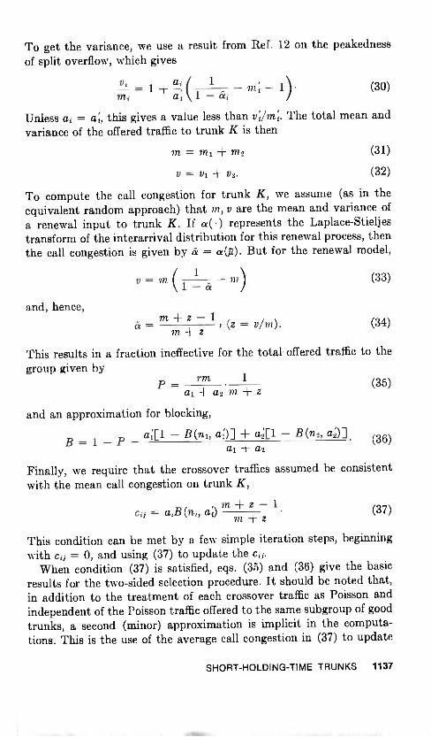
To get the variance, we use a result from Ref. 12 on the peakednessof split overflow, which gives
vi 1
i a ik 1 -m - 1) (30)
Unless ai = a;, this gives a value less than v;/m;. The total mean andvariance of the offered traffic to trunk K is then
= 1111 ± 1112
V = vl + V2.
(31)
(32)
To compute the call congestion for trunk K, we assume (as in theequivalent random approach) that m, v are the mean and variance of
a renewal input to trunk K. If a( ) represents the Laplace-Stieljestransform of the interarrival distribution for this renewal process, thenthe call congestion is given by a = a (A). But for the renewal model,
and, hence,
V = 1111 in)
k -_ z - 1a=
z(z = v/m).
(33)
(34)
This results in a fraction ineffective for the total offered traffic to the
group given byillP - r
a2 z(35)
and an approximation for blocking,
a;[1. - B(ni, a;)] - B(n2, as)]B= 1 -P - (36)a2
Finally, we require that the crossover traffics assumed be consistentwith the mean call congestion on trunk K,
1cif = aiB(ni, a1)
z - (37)z
This condition can be met by a few simple iteration steps, beginningwith ci; = 0, and using (37) to update the cif.
When condition (37) is satisfied, eqs. (35) and (36) give the basicresults for the two-sided selection procedure. It should be noted that,in addition to the treatment of each crossover traffic as Poisson andindependent of the Poisson traffic offered to the same subgroup of goodtrunks, a second (minor) approximation is implicit in the computa-tions. This is the use of the average call congestion in (37) to update
SHORT -HOLDING -TIME TRUNKS 1137
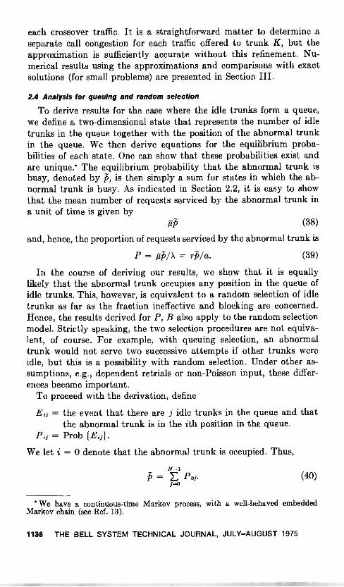
each crossover traffic. It is a straightforward matter to determine aseparate call congestion for each traffic offered to trunk K, but theapproximation is sufficiently accurate without this refinement. Nu-merical results using the approximations and comparisons with exactsolutions (for small problems) are presented in Section III.
2.4 Analysis for queuing and random selection
To derive results for the case where the idle trunks form a queue,we define a two-dimensional state that represents the number of idletrunks in the queue together with the position of the abnormal trunkin the queue. We then derive equations for the equilibrium proba-bilities of each state. One can show that these probabilities exist andare unique.* The equilibrium probability that the abnormal trunk isbusy, denoted by fo, is then simply a sum for states in which the ab-normal trunk is busy. As indicated in Section 2.2, it is easy to showthat the mean number of requests serviced by the abnormal trunk ina unit of time is given by
rifi (38)
and, hence, the proportion of requests serviced by the abnormal trunk is
P = = rf)/a. (39)
In the course of deriving our results, we show that it is equallylikely that the abnormal trunk occupies any position in the queue ofidle trunks. This, however, is equivalent to a random selection of idletrunks as far as the fraction ineffective and blocking are concerned.Hence, the results derived for P, B also apply to the random selectionmodel. Strictly speaking, the two selection procedures are not equiva-lent, of course. For example, with queuing selection, an abnormaltrunk would not serve two successive attempts if other trunks wereidle, but this is a possibility with random selection. Under other as-sumptions, e.g., dependent retrials or non -Poisson input, these differ-ences become important.
To proceed with the derivation, define
Ei; = the event that there are j idle trunks in the queue and thatthe abnormal trunk is in the ith position in the queue.
Pi; = Prob 1E111.
We let i = 0 denote that the abnormal trunk is occupied. Thus,
N-1= E Poi. (40)
We have a continuous -time Markov process, with a well-behaved embeddedMarkov chain (see Ref. 13).
1138 THE BELL SYSTEM TECHNICAL JOURNAL, JULY-AUGUST 1975

The following equations can be readily derived relating the Pii's :
EA. (N - 1);dPoo = XP01 (41)
CA (N - j - 1)11 + x1P01 = xPo,3+1 + (N - DAPod-ifor 1 < j < N - 1, (42)
X1P0,N-1 = XP1N APo,N-2) (43)
- X1P.-; = (N - 1)APi,1_1 XPi+1,1+1
for 0<i<j.N, (44)
UN - .i)/2 + = 11P0,;_1 + X/3J+1,,.÷1
for 0 < j < N, (45)
and, trivially,Pi; = 0 for i > j, or j > N;Poi = 0 for j N.
These equations appear quite formidable because of the apparent lackof simple structure. A brute force algebraic approach seems unfruitful,as does a generating function approach.
Instead, we make the conjecture that
P13= P2j = ' =P;; for all j 1. (46)
We should note that (46) is equivalent to assuming that the idletrunk is selected at random. This is true because Pi; represents theprobability of seeing the state (i, j) at a random instant in equilibriumand Poisson arrivals see the same distribution.
We justify our conjecture by using (46) in (41) to (45) togetherwith the fact that the probabilities must add to 1 and showing thatthe resulting equations have a simple solution. This solution can besubstituted into the original equations to show that we indeed havethe correct solution. However, since there exists a unique equilibriumsolution to these equations and we have, in effect, solved them byadding additional constraints, the proof is complete without this step.
Proceeding in the manner described, we first use (46) in (41) to (45)and obtain the following equations :
CA (N - 1)A1Poo = XPoi (47)
CA (N - j - 1)12 + xipo; = + (N Aid3o,J-1 XPJ+1.J+1for 1 j < N - 1, (48)
CA XiPo,N-1 = XPNN AP0,N-2, (49)
UN - + X = (N - .1+ 1)03.i_1,;_1 +for 0 < j < N, (50)
SHORT -HOLDING -TIME TRUNKS 1139

and[(N - ± XiPi; = 11Poi-1 XPi+1,J+1
for 0 < j =< N. (51)
Putting j = N in eq. (50), recalling that P N+1,N+1 = 0, we get
P N -1,N-1 = PNN = aP NN (52)
Repeatedly reducing j by 1 and solving for in terms of PNN,we get
a,v-;Pj = PNN, 1, , N. (53)
(N - j)!
Using (53) in (51) results in
X aANP05 = P N
(117 - - 1) !
Finally, from (47) we getaN-1
Poo - P N(N - 1) !
(54)
(55)
One can check that expressions (53), (54), and (55) satisfy eqs. (48)and (49), which proves the conjecture.
We compute PNN from the fact that the sum of the probabilitiesmust be 1. This yields
r aN IN- j1V-1 N 1,1
aiN +NT/1)-F +1]. (56)
Thus,
and
N-1 a;Ata E -N -1 j=0E Po, -
5=0 AN EN a.j ( N 1
N-1 ai
P - 7.15 - 5=0
a N ai /N -j j j )'N ;=0 j! N rN
recalling that r = 12/12.
1140 THE BELL SYSTEM TECHNICAL JOURNAL, JULY -AUGUST 1975
(57)
(58)
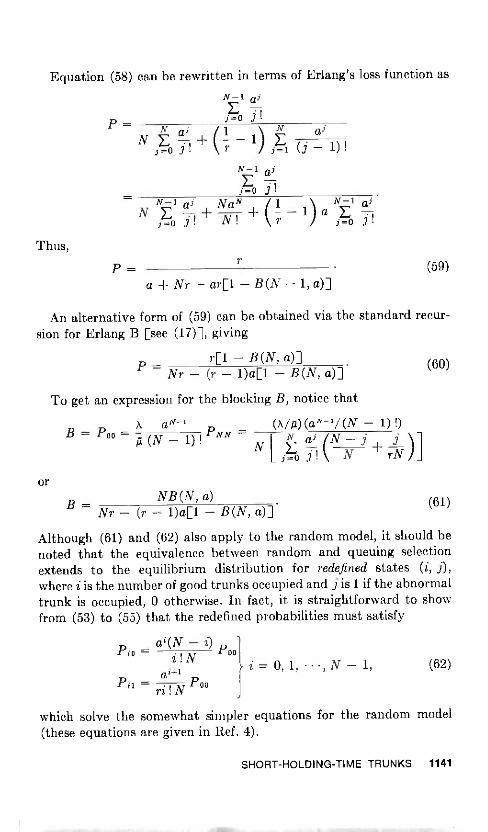
Equation (58) can be rewritten in terms of Erlang's loss function as
Thus,
P=
N -1 jaj=0 3
ajN =aj / _ \ -'1N4
j .1! r (j - 1)
N a' NaN (1 N -I a;N ,
J=0 ./ . A !- 1) a
=o
'P = 7 (59)
a + Nr - arE1 -B (N -L
An alternative form of (59) can be obtained via the standard recur-sion for Erlang B [see (17)], giving
?D. - B(N, a)]P = (60)Nr - (r - 1)a[1. - B(N, a)]
To get an expression for the blocking B, notice that
X a N-1 (X/p)(aN-7(N - 1) !)B - Poo = P N N(IV - 1) ! aj iN - j j
L .fr=0 j! N rN
Or
NB (N , a)B = (61)
Nr - (r - 1)a[1 - B(N, a)]Although (61) and (62) also apply to the random model, it should benoted that the equivalence between random and queuing selectionextends to the equilibrium distribution for redefined states (i, j),where i is the number of good trunks occupied and j is 1 if the abnormaltrunk is occupied, 0 otherwise. In fact, it is straightforward to showfrom (53) to (55) that the redefined probabilities must satisfy
Pi0 = 00N i = 0, 1, , N - 1, (62)ai+'
Pil = Poori! N
which solve the somewhat simpler equations for the random model(these equations are given in Ref. 4).
SHORT -HOLDING -TIME TRUNKS 1141

III. NUMERICAL RESULTS
This section presents selected numerical results obtained with thesolution procedures of Section II.
3.1 Ordered selection (Figs. 2 to 5)
Figure 2 gives the fraction ineffective for r = 5 and the blocking* forr = 5, N = 20. Even for this relatively small value of r, the short -holding -time trunk has a significant impact, which decreases as the positionin the order of selection increases. For large values of offered load, thedependence of fraction ineffective on K (position of the short -holding -time trunk) is decreased. In fact, it follows from Little's Law° that,for all K (and all selection procedures), P r/a, with the boundapproached as the time congestion on the short -holding -time trunkapproaches 1.0; i.e., for very large a. For a = 25, K = 1, we note thatP= 0.17, r/a = 0.2.
The results for fraction ineffective do not depend on the totalnumber of trunks N > K. For blocking, N is important. For N = 20,r = 5, blocking is decreased from Erlang B blocking by about s in the(design) range for 20 to 30 percent overflow, with the decrease rela-tively insensitive to K. Blocking results are approximate, with errorsresulting only from the application of the equivalent random method.In cases where exact solutions were compared to the approximate,the agreement was good. The decreased overflow resulting from ashort -holding -time trunk can contribute substantial errors in estima-tion procedures for which overflow enters. Usage measurements arealso affected by a short -holding -time trunk, with mean carried usagegiven by aP/r a(1 -P - B).
Figure 3, for r = 15, is similar to Fig. 2, but with larger impactsand more spread between the curves. The ratio r = 15 is typical for ashort -holding -time trunk and shows that P > 0.4 can easily occur,even for relatively large loads. The limiting ratio r = co (zero -holding -time trunk) would result in Pa° = B(K - 1, a), and B°' = 0, whichare substantially different from the r = 15 results. For example,P°°= 1 for K = 1.
3.2 Two-sided selection (Figs. 4 and 5)
Figure 4 gives the behavior for N = 5, r = 15, including a com-parison with the exact solution obtained by solving the state equationsfor the system. The approximation for P displays essentially no errorfor low blocking. This is to be expected for conditions under which the
" Recall that blocking refers to the fraction of attempts that find all trunks busy inthe group, whether or not it is a final or high -usage group.
1142 THE BELL SYSTEM TECHNICAL JOURNAL, JULY-AUGUST 1975
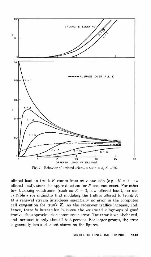
0.2
B
0.1
P
0
1.0
0.8
0.6
0.4
0.2
0
0 5
ERLANG B BLOCKING
10 15 20
OFFERED LOAD IN ERLANGS25
Fig. 2-Behavior of ordered selection for r = 5, N = 20.
30
offered load to trunk K comes from only one side (e.g., K = 1, lowoffered load), since the approximation for P becomes exact. For otherlow blocking conditions (such as K = 3, low offered load), no dis-cernible error indicates that modeling the traffics offered to trunk Kas a renewal stream introduces essentially no error in the computedcall congestion for trunk K. As the crossover traffics increase, and,hence, there is interaction between the separated subgroups of goodtrunks, the approximation shows some error. The error is well-behaved,and increases to only about 2 to 3 percent. For larger groups, the erroris generally less and is not shown on the figures.
SHORT -HOLDING -TIME TRUNKS 1143

B
0.2
0.1
0
5 10 15 20
OFFERED LOAD IN ERLANGS
25
Fig. 3-Behavior of ordered selection for r = 15, N = 20.
30
Errors in the blocking are larger. Since peakedness is ignored indeterminining the crossover traffics and the carried load on the goodtrunks, this is to be expected. However, the absolute error does notincrease significantly with offered load. As the change from Erlang Bblocking is the important factor in applications, this error behavior isacceptable. As for ordered selection, the blocking is relatively insensi-tive to K.
The interesting behavior for K = 1 is apparently due to the sizeof the group. For K = 1, N 2, qualitatively, one would expect thatthe fraction ineffective seen by load al monotonically decreases from
1144 THE BELL SYSTEM TECHNICAL JOURNAL, JULY-AUGUST 1975
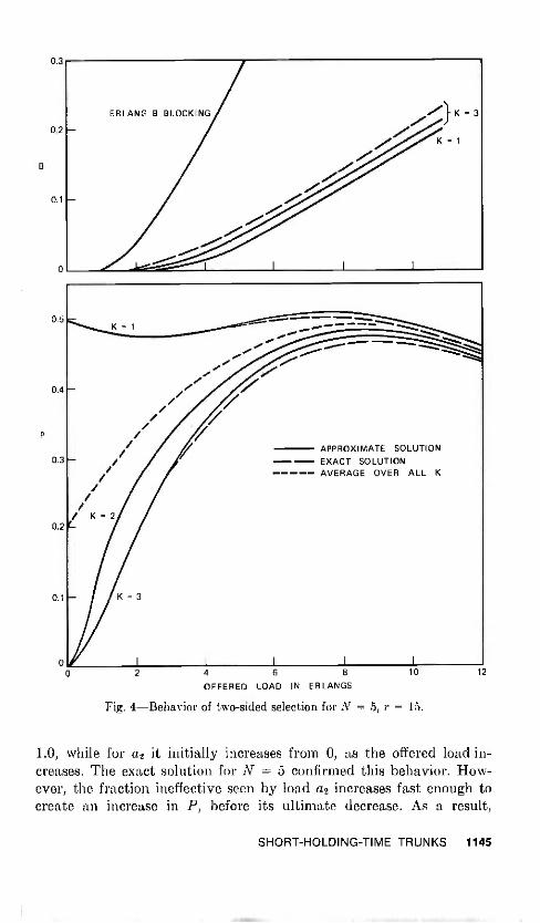
B
P
0.5
0.4
0.3
0.2
0.1
ERLANG B BLOCKING
APPROXIMATE SOLUTION-- EXACT SOLUTION
AVERAGE OVER ALL K
=3
2 4 6 8 10 12
OFFERED LOAD IN ERLANGS
Fig. 4-Behavior of two-sided selection for N = 5, r = 15.
1.0, while for a2 it initially increases from 0, as the offered load in-creases. The exact solution for N = 5 confirmed this behavior. How-ever, the fraction ineffective seen by load a2 increases fast enough tocreate an increase in P, before its ultimate decrease. As a result,
SHORT -HOLDING -TIME TRUNKS 1145
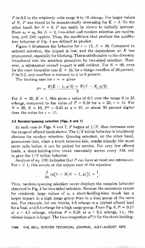
P 0.5 in the relatively wide range 0 to 10 erlangs. For larger valuesof N, P was found to be monotonically decreasing for K = 1. On theother hand, for N = 2, P can easily be shown to initially increase.Since al = a2, for N = 2, two-sided and random selection are equiva-lent, and (59) applies. Thus, the conditions that produce the qualita-tive behavior of Fig. 4 are difficult to predict.
Figure 5 illustrates the behavior for r = 15, N = 20. Compared toordered selection, the impact is less, and the dependence on K lesspronounced, especially for blocking. This is attributable to the diversityintroduced into the selection procedure by two-sided selection. How-ever, a substantial overall impact is still evident. For N = 20, evenfor the most favorable case K = 10, for a design overflow of 20 percent,P 0.2, and overflow is reduced to 5 to 6 percent.
The limiting case for r = oc gives
B(K - 1, a/2) B(N - K, a/2)=
2
For N = 20, K = 1, this gives a value of 0.5 over the range 0 to 25erlangs, compared to the value of P = 0.29 for a = 25, r = 15. ForN = 20, K = 10, P°' = 0.35 at a = 25, or about 50 percent higherthan the value for r = 15.
3.3 Random/queuing selection (Figs. 6 and 7)
In each case in Figs. 6 and 7, P begins at 1/N, then increases overthe range of offered loads shown. The 1/N initial behavior is intuitivelyobvious for random selection. Queuing selection, on the other hand,guarantees that, when a trunk becomes idle, trunks already idle mustserve calls before it can be picked for service. For very low offeredloads, a short -holding -time trunk essentially serves every Nth callto give the 1/N initial behavior.
Analysis of eq. (59) indicates that P can have at most one extremum.For r > 1, this occurs at the unique root of the equation
a{ aE1 - B(N -L ---
Thus, random/queuing selection never displays the complex behaviorobserved in Fig. 4 for two-sided selection. Because the extremum occursfor relatively large values of a, a short -holding -time trunk has alarger impact in a high usage group than in a final group of the samesize. For example, for ten trunks, 4.5 erlangs is a typical offered loadfor a final, and 9.5 erlangs for a high usage group. From Fig. 6, P = 0.17at a = 4.5 erlangs, whereas P = 0.28 at a = 9.5 erlangs, i.e., therelative impact is larger. The time congestion aP/r for the short -holding -
1146 THE BELL SYSTEM TECHNICAL JOURNAL, JULY-AUGUST 1975

B
P
0.3
0.2
0.1
0
0.5
0.4
0.3
0.2
0.1
=1
=5
K = 10
5
---- AVERAGE OVER ALL K
10 15 20
OFFERED LOAD IN ERLANGS25 30
Fig. 5-Behavior of two-sided selection for N = 20, r = 15.
time trunk is 0.052 at a = 4.5 erlangs, and 0.175 at a = 9.5 erlangs,i.e., the absolute impact of the short -holding -time trunk is over threetimes as much for the high -usage application. In terms of the expectedtime congestion with a short -holding -time trunk equally likely in anyposition, this general behavior also holds for two-sided and orderedselection. This follows from the increase in average fraction ineffectiveas the offered load increases.
SHORT -HOLDING -TIME TRUNKS 1147

8
0.3
0.2
0.1
0
0.5
0.4
0.3
0.2
0.1
0
0 5 10 15 20
OFFERED LOAD IN ERLANGS26
Fig. 6-Behavior of random selection for r = 15, N = 5, 10, 20.
30
Figure 7 displays the behavior of random/queuing selection as rvaries. In all cases, P is close to its maximum over a fairly wide range.The limiting case r = 00 gives [see (59)]
Pc° - N - aD. - B(N - 1, a)]For N = 20, a = 25 erlangs, Pc° = 0.36, compared to the r = 20
1148 THE BELL SYSTEM TECHNICAL JOURNAL, JULY-AUGUST 1975
1

B
P
0.3
0.2
0.1
0
0.3
0.2
0.1
ERLANG B BLOCKING r = 5
= 10
= 15
= 20
r = 20r = 15
= 10
r = 5
10 15 20
OFFERED LOAD IN ERLANGS
25
Fig. 7-Behavior of random selection for N = 20, r = 5, 10, 15, 20.
30
value from Fig. 7 of P = 0.23. Since P is no more difficult to computethan Px, the upper bound Px is of limited use in this case.
3.4 Comparison of selection procedures
To compare selection procedures, the measure taken is the expectedvalue of P, denoted by P, given that a short -holding -time trunkis equally likely in any position. Computationally, it was found that
Random'or Two-sided Orderedqueuing selection = selection '
selection
with equality occurring only at a = 0. Figure 8 for N = 20, r = 15 dis-plays typical behavior. The differences are substantial. It is likely that
SHORT -HOLDING -TIME TRUNKS 1149

0.3
0.2p-
i
0.1
P
ERLANG B BLOCKING
10 15 20
OFFERED LOAD IN ERLANGS
RANDOM
TWO-SIDEDAND ORDERED
25 30
Fig. 8-Comparison of selection procedures for short -holding -time trunk equallylikely in any position (N = 20, r = 15).
any improvement over the random/queuing behavior would requirea selection procedure based on more information. For example,choosing the idle trunk whose last holding time was longest wouldfurther reduce the impact of a short -holding -time trunk.
The expected blocking does not show much difference from one selec-tion procedure to another, but all disciplines show a substantial reduc-tion from the Erlang B results.
3.5 Validation remarks
The basic traffic assumptions of the model concern holding timesand the arrival process. For normal trunk holding times (which resultfrom a mix of conversations, busys, don't answers), the exponentialassumption is reasonable. For short -holding -time trunks, this assump-tion may be less valid. For example, trunks resulting in immediate
1150 THE BELL SYSTEM TECHNICAL JOURNAL, JULY-AUGUST 1975
reorder returned to the customer would not likely display the expo-nential behavior. However, since the Erlang B formula holds forarbitrary holding -time distributions, it is reasonable to expect that theresults should not be too sensitive to the form of the distribution.
The Poisson assumption for the arrival process can be invalidateddue to time variations, to peakedness (for groups receiving overflowtraffic), or to retrial behavior. For ordered selection with K = 1,peakedness clearly reduces the impact of a short -holding -time trunk.This behavior may be reversed for higher values of K since peakednessincreases the mean attempt rate to trunk K. For example, for r = 00,K >= 2, P is increased. However, several peaked traffic computationsfor r = 15 give values of the fraction ineffective that are very closeto the Poisson value.
Even if the Poisson assumption is valid with all trunks good, it canbe violated in the presence of a short -holding -time trunk. The shorttime between a retrial and the failure that initiated it gives the retriala high probability of meeting the same conditions as the initial failure.For two-sided, ordered, and random selection, this could increase theimpact of the short -holding trunk over what would be expected froma Poisson assumption.
The model is also susceptible to variations from the idealized selec-tion procedures. This holds particularly for applications to oldersystems where grading and multipling arrangements can lead to manydifferent selection procedures. It also holds for applications to 5XBsystems, where any irregularity in the distribution of trunks on theframes can distort the selection procedure from the idealized randomselection model. In fact, individual circuit usage results would seem toindicate that significant discrepancies from (cyclic) random selectionmay be quite common in 5XB. Thus, for any specific application,suitability of the model would have to be determined.
Figure 9 shows data obtained by special measurements from a Cross-bar Tandem group containing a short -holding -time trunk. The pegcount and usage measurements during the study hour indicate thattrunk 2 had a short holding time relative to other trunks in thegroup, and a failure condition was subsequently verified. Thus, all35 attempts on the trunk are assumed to have failed. The large im-balance in the offered attempts from either side of the group could bestatistical, or it could be due to irregularities in incoming trunkassignment to frames (which determines the order of selection). It ismore likely due to retrials. Thus, the reasonable assumption thatal = a2 can be violated in some situations.
Since the measured hour was not the busy hour, the left side of thegroup can be treated like ordered selection. The estimate for a mean
SHORT -HOLDING -TIME TRUNKS 1151
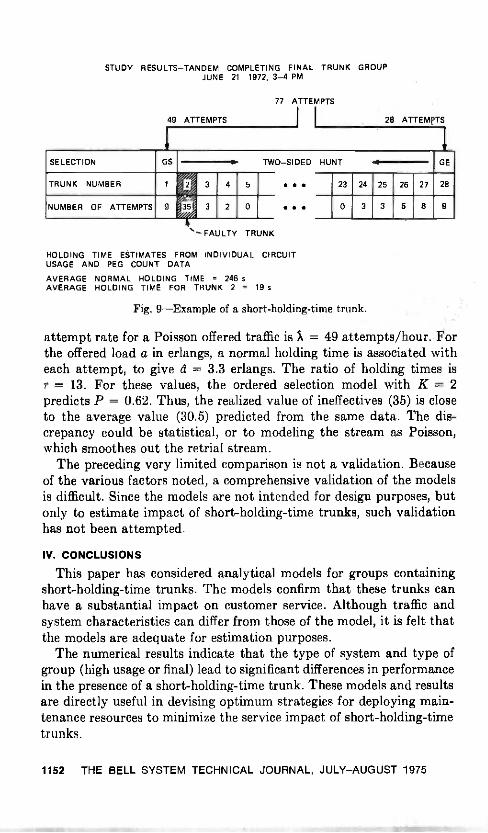
STUDY RESULTS-TANDEM COMPLETING FINAL TRUNK GROUPJUNE 21 1972, 3-4 PM
49 ATTEMPTS
77 ATTEMPTS
I I28 ATTEMPTS
SELECTION GS TWO-SIDED HUNT
TRUNK NUMBER 2
NUMBER OF ATTEMPTS 35
- FAULTY TRUNK
HOLDING TIME ESTIMATES FROM INDIVIDUAL CIRCUITUSAGE AND PEG COUNT DATA
AVERAGE NORMAL HOLDING TIME = 246 sAVERAGE HOLDING TIME FOR TRUNK 2 = 19 s
GE
23 24 25 26 27 28
9
Fig. 9-Example of a short -holding -time trunk.
attempt rate for a Poisson offered traffic is X = 49 attempts/hour. Forthe offered load a in erlangs, a normal holding time is associated witheach attempt, to give a = 3.3 erlangs. The ratio of holding times isr = 13. For these values, the ordered selection model with K = 2predicts P = 0.62. Thus, the realized value of ineffectives (35) is closeto the average value (30.5) predicted from the same data. The dis-crepancy could be statistical, or to modeling the stream as Poisson,which smoothes out the retrial stream.
The preceding very limited comparison is not a validation. Becauseof the various factors noted, a comprehensive validation of the modelsis difficult. Since the models are not intended for design purposes, butonly to estimate impact of short -holding -time trunks, such validationhas not been attempted.
IV. CONCLUSIONS
This paper has considered analytical models for groups containingshort -holding -time trunks. The models confirm that these trunks canhave a substantial impact on customer service. Although traffic andsystem characteristics can differ from those of the model, it is felt thatthe models are adequate for estimation purposes.
The numerical results indicate that the type of system and type ofgroup (high usage or final) lead to significant differences in performancein the presence of a short -holding -time trunk. These models and resultsare directly useful in devising optimum strategies for deploying main-tenance resources to minimize the service impact of short -holding -timetrunks.
1152 THE BELL SYSTEM TECHNICAL JOURNAL, JULY-AUGUST 1975

V. ACKNOWLEDGMENTS
The authors gratefully acknowledge comments by S. Horing, dis-
cussions with M. F. Morse on trunk selection, and the programmingassistance of Mary Zeitler and Anne Vottero. Data for the Fig. 9 ex-ample were supplied by J. L. Laude.
REFERENCES
1 L. J. Forys and E. J. Messerli, "Analysis of Trunk Groups with a Short HoldingTime Trunk," unpublished work.
2. R. I. Wilkinson, "Theories for Toll Traffic Engineering in the U. S. A.," B.S.T.J.,35, No. 2 (March 1956), pp. 421-514.
3. Andrezej Klimontowicz, "Grade of Service for Full Available Trunk Groups withFaulty Trunks," Proceedings of the 6th International Teletraffic Conference,Munich, 1970, pp. 212/1-212/6.
4. P. J. Bogert, W. S. Gifford, and I. J. Shapiro, "Directed Maintenance: TroublesEncountered in Placing DDD Calls," unpublished work.
5. L. J. Forys, "Occupancy Probabilities for an Ordered Hunt Group with UnequalService Times," unpublished work.
6. A. Descloux, "On Overflow Processes of Trunk Groups with Poisson Input andExponential Service Time," B.S.T.J., 42, No. 2 (March 1963), pp. 388-397.
7. W. S. Gifford and J. Shapiro, "Effect of the Change in Mean Holding TimeAssociated with an Equipment Irregularity on Network Trouble Detectionand Customer Service," IEEE Trans. Communications, COM-21, No. 1(January 1973), pp. 1-6.
8. J. S. Kaufman, "Distribution of Busy Trunks in a Random Hunt Group Con-taining Killer Trunks," unpublished work.
9. J. D. C. Little, "A Proof of the Queueing Formula: L = NW," Operations Re-search, 9, No. 3 (May -June 1961), pp. 383-87.
10. J. Riordan, Stochastic Service Systems, New York : John Wiley, 1962.11. L. Taktics, Introduction to the Theory of Queues, New York: Oxford University
Press, 1962.12. A. Descloux, "On the Components of Overflow Traffic," unpublished work.13. J. G. Kemeny and J. L. Snell, Finite Markov Chains, Princeton, N. J.: Van
Nostrand, 1960.
SHORT -HOLDING -TIME TRUNKS 1153

la1104.111.111.1MilaNii.4.10: Was . 411111011111111kailiam,

Copyright 1975 American Telephone and Telegraph CompanyTHE BELL SYSTEM TECHNICAL JOURNAL
Vol. 54, No. 6, July -August 1975Printed in U.S.A.
Entropy Measurements for Nonadaptive andAdaptive, Frame -to -Frame, Linear -
Predictive Coding of Video -telephone Signals
By B. G. HASKELL(Manuscript received January 7, 1975)
Linear predictive coding is an efficient method for transmitting theamplitudes of moving -area picture elements (pets) in a conditional re-plenishment coder for video -telephone signals. It has been conjectured thatif the linear predictor can dynamically adapt to the speed and direction ofmotion in the scene, then greatly improved performance should result. Totest this conjecture and to get a first -order estimate of the possible saving,computer simulations were carried out using pairs of video -telephoneframes stored on digital discs. Using this data, picture quality could notbe studied. However, differential signal entropies could be estimated, andthis was done for several nonadaptive and adaptive linear predictors.Entropies (in bits per moving -area pel) for adaptive linear predictorswere significantly lower than for nonadaptive predictors, indicating thatsubstantial bit -rate savings should be possible. However, simpler imple-mentations will have to be devised before adaptive prediction becomespracticable.
I. INTRODUCTION
In coding television pictures for transmission over a digital channel,it is well known that the required bit rate can be significantly reducedby removing various redundancies that exist in the signal, and inrecent years methods for removing frame -to -frame redundancy havebeen investigated.' In a conditional replenishment' system, only thepicture elements (pels) that have changed significantly since theprevious frame are transmitted. Their amplitudes as well as theirlocations must be sent ; however, most of the transmission capacityis used in sending the amplitudes. During periods of rapid motion, onlyevery other moving -area pel need be transmitted, i.e., the moving areaof the picture can be subsampled3,4 at half -rate with the unsampledpels being replaced by the average of their neighbors.
1155

Linear predictive coding is an efficient method of transmitting theseamplitudes. Channel rates of 1 bit per pel and below have been ob-tained.4-7 With this technique, a prediction is formed of each pel tobe sent by computing a linear combination of previously transmittedpels. The difference between the actual value and prediction is thenquantized and coded for transmission. Since the differential signal issmall usually and large only occasionally, variable word -length codingcan be used to good advantage in reducing the overall bit rate.
The entropy of the quantized moving -area differential signal pro-vides an estimate of the average number of bits required to transmita pel. Thus, it is a good yardstick for comparing the performance of
various frame -to -frame predictive coders. The entropy will depend onthe amount of detail (frequency and amplitude of brightness varia-tions) in the moving area of a frame as well as on the speed of move-ment in the scene. The overall bit rate, however, is strongly dependenton the number of pels in the moving area which, in turn, is deter-mined by the type of picture to be transmitted. See Ref. 8 for statisticson the number of moving -area pels per frame in typical video -telephonesignals.
In Refs. 9 and 10, and by simple extension of the techniques of Ref.11, it is suggested that if the predictor can dynamically adapt to thespeed and direction of motion in the scene, then greatly improvedperformance should result. For example, if an object is moving leftto right at a speed of about 1 pel per frame period (PEF) then for eachmoving -area pel of the present frame a very good prediction shouldbe obtainable by going back to the previous frame and looking 1 pelto the left. Other types of adaptive linear prediction are described inRefs. 12 to 14. They suggest that the weighting coefficients in thelinear predictor be varied adaptively to make the differential signalsmaller.
II. COMPUTER SIMULATION
To get some comparison between nonadaptive and adaptive, frame -to -frame, linear predictors, computer simulations were carried outusing about three dozen video -telephone picture sequences stored as8 -bit PCM on digital disc (two successive frames per sequence). Withonly two frames available per sequence, picture quality could not bestudied. However, moving -area differential signal entropies could beestimated, and this was done for several nonadaptive and adaptivepredictors.
Characteristics: 30 -Hz frame -rate, 271 lines, 2:1 interlace, 3 dB down at 1 MHz,2 -MHz sampling -rate, 8 bits/sample, 210 visible samples/line.
1156 THE BELL SYSTEM TECHNICAL JOURNAL, JULY-AUGUST 1975
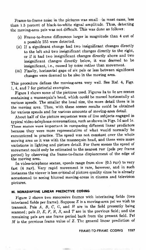
Frame -to -frame noise in the pictures was small-in most cases, lessthan 1.5 percent of black -to -white signal amplitude. Thus, detectingthe moving -area pels was not difficult. This was done as follows :
(i) Frame -to -frame differences larger in magnitude than 4 out ofa possible 255 were detected.
(ii) If a significant change had two insignificant changes directlyto the left and two insignificant changes directly to the right,or if it had two insignificant changes directly above and twoinsignificant changes directly below, it was deemed to beinsignificant, i.e., caused by noise rather than movement.
(iii) Finally, horizontal gaps of six pels or less between significantchanges were deemed to be also in the moving area.
This procedure defines the moving -area very well. See Ref. 4, Figs.1, 4, and 7 for pictorial examples.
Figure 1 shows some of the pictures used. Figures la to lc are scenescontaining a mannequin's head, which could be moved horizontally atvarious speeds. The smaller the head size, the more detail there is inthe moving area. Thus, with these scenes results could be obtainedfor various speeds and for various amounts of moving -area detail.
About half of the picture sequences were of live subjects engaged intypical video -telephone conversations, such as shown in Figs. ld and le.These scenes were important in comparing different linear predictorsbecause they were more representative of what would normally beencountered in practice. The speed was not constant over the wholemoving area as it was with the mannequin head, and there were morevariations in lighting and picture detail. For these scenes the speed ofmovement could only be estimated to the nearest PEF (pels per frameperiod) by observing the frame -to -frame displacement of the edge of
the moving area.In video -telephone scenes, speeds range from slow (0.5 PEF) to very
fast (4 PEF). Very rapid movement is rare, however, and in suchinstances the viewer is less critical of picture quality since he is alreadyaccustomed to seeing blurred moving -areas in cinema and televisionpictures.
III. NONADAPTIVE LINEAR PREDICTIVE CODING
Figure 2 shows two successive frames with interlacing fields (twointerlaced fields per frame). Suppose Z is a moving -area pel we wish totransmit. Pels A, B, C, G, and H are in the field presently beingscanned ; pels D, E, F, R, S, and T are in the previous field ; and theremaining pels are one frame period back from the present field. PelM is the previous frame value of Z. The general linear prediction of
FRAME -TO -FRAME CODING 1157
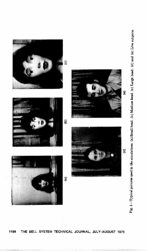
(a)
(d)
(b)
(e)
(c)
Fig.
1-T
ypic
al p
ictu
res
used
in th
e si
mul
atio
ns. (
a) S
mal
l hea
d. (
b) M
ediu
m h
ead.
(c)
Lar
ge h
ead.
(d)
and
(e)
Liv
e su
bjec
ts.

PRESENTFIELD :.- D E F
......- -311. A B C
::....PE LS
..........41
---- a. G H ®R S T'dir-
I J
\ PREVIOUSU LON V.* - -) FRAME
// PE LS- - -
0 P Q
***".PREVIOUS'FIELD
PE LS
Fig. 2-Two successive television frames with interlacing assumed (two interlacedfields per frame). Pels Z and M are exactly one frame period apart.
Z based on the previously transmitted pels, which are nearby bothspatially and temporally, is given by
Pz = a1A + a2B a3C + + a22V, (1)
where al, a2, , a22 are the weighting coefficients.Since Z is 8 -bit PCM and Pz is clipped to 8 -bit PCM, the differential
signal Z-Pz can assume any of 511 levels. The entropy of the 511 -levelsignal is a measure of the relative performance of different predictors.However, in practice, a more coarsely quantized signal (consistentwith acceptable picture quality) would probably be transmitted toreduce the overall bit rate.
Picture quality could not be observed in the simulations. However,to get a rough estimate of bit rate for linear predictors with coarserquantization, a compromise 35 -level' quantization scale was chosenthat is slightly coarser than the quantizer of Ref. 4 for frame differ-ences and somewhat finer than the one used in Ref. 7 during periodsof movement for element differences. Using this quantization scale,slope overload rarely occurs, and the predominant picture degradationis granular noise in the moving areas. This has been verified in recentpreliminary simulations using thirty consecutive frames stored ondigital disc. Using the nonadaptive and adaptive linear predictorsmentioned in this paper, there is little difference in picture qualityin the limited picture sample studied. However, much work remains tobe done in this area.
On a scale of 0 to 255, the levels are: 0, ±5, ±14, ±22, ±30, ±40, ±50, ±60,±70, ±82, ±94, ±106, ±118, ±130, ±142, ±154, ±166, and ±178.
FRAME -TO -FRAME CODING 1159

The effects of the predictive coder feedback loop are ignored inthe entropy measurements. Feedback can affect results to a significantdegree if quantization is extremely coarse. Even so, the entropy mea-surements reported here are in close agreement with those of Refs.4 and 7.
For various nonadaptive linear predictors, Figs. 3 to 8 show theentropy (bits per moving -area pel) of the differential signal as a func-tion of the speed of movement (pels per frame period or PEFs). Resultsare summarized in Table I. For these cases, more moving -area detail(smaller head) resulted in somewhat higher entropies, as would beexpected, but moving -head results were still fairly close to each other.The live -subject entropies were close to the moving -head entropies forthe most part, even though there was considerable variation in moving -area picture detail.
6
5
4
3
2
1
0
......---'
A
1
A
A
A
...-..."'
A
t511 LEVELS
..---35 LEVELS
117
0 LARGE HEADX SMALL HEAD0 MEDIUM HEADA LIVE SUBJECTS
1
0 0.5 1.0 1.5 2.0 2.5 3.0 3.5 4 0
SPEED IN PELS PER FRAME INTERVAL (PEF)
Fig. 3-Entropy of the frame difference signal in the moving area versus speed.Pz = M. Starting with 8 -bit PCM as was done in these simulations the differentialsignal could assume any of 511 levels. Results are also shown for coarser quantization.to 35 levels which still gives very good picture quality. Solid curves are for the man-nequin head at various distances from the camera. Unconnected points are for livesubjects, such as in Figs. ld and le.
1160 THE BELL SYSTEM TECHNICAL JOURNAL, JULY-AUGUST 1975
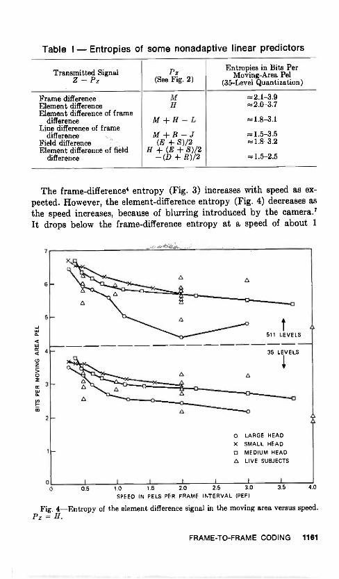
Table I - Entropies of some nonadaptive linear predictors
Transmitted SignalZ - Pz
Pz(See Fig. 2)
Entropies in Bits PerMoving -Area Pel
(35 -Level Quantization)
Frame differenceElement differenceElement difference of frame
differenceLine difference of frame
differenceField differenceElement difference of field
difference
MH
M H -LM B -J(E S)/2
H (E S)/2- (D R)/2
2.1-3.9=2.0-3.7
1.8-3.1
- 1.5-3.51.8-3.2
1.5-2.5
The frame -difference' entropy (Fig. 3) increases with speed as ex-pected. However, the element -difference entropy (Fig. 4) decreases asthe speed increases, because of blurring introduced by the camera.'It drops below the frame -difference entropy at a speed of about 1
7
6
5
4
3
2
0
0 LARGE HEADX SMALL HEADCI MEDIUM HEADA LIVE SUBJECTS
0 0.5 1.0 1.5 2.0 2.5 3.0
SPEED IN PELS PER FRAME INTERVAL (PEF)
Fig. 4-Entropy of the element difference signal in the moving area versus speed.Pz = H.
3.5 4.0
FRAME -TO -FRAME CODING 1161

PEF.7 Subsampling at half -rate, however, causes it to rise above thelevels shown in Fig. 4.
The element difference of frame -difference entropy" and line differ-ence of frame -difference entropy'6 (Figs. 5 and 6) are very close toeach other even though with interlace (see Fig. 2) the previous line isfurther away from pel Z than is the previous element. D. J. Connorhas pointed out that this occurs because movement in the scenes ismostly in the horizontal direction. However, the line -difference offrame -difference signal has the advantage of being unaffected bysubsampling along the line.
The field -difference entropy" (Fig. 7) is lower than the frame -differ-ence entropy, except at very slow speeds, because of the spatial andtemporal closeness of the previous field pels. It compares well evenwith the double derivative signal of Figs. 5 and 6. The element differ-ence of field -difference entropy (Fig. 8) is smaller than any of theothers and, other factors ignored, would be the logical choice in a non -adaptive, frame -to -frame, linear predictive coder. However, sub -
7
6
5
4
3
2
1
0
A
A
A
A
x-11--.44-----4< A 0
iA
A
O
AG a
a
t511 LEVELS
35 LEVELS
O
0 LARGE HEADX SMALL HEAD0 MEDIUM HEADA LIVE SUBJECTS
aAa
aa
0 0.5 1.0 1.5 2.0 2.5 3.0 3.5 4.0
SPEED IN PELS PER FRAME INTERVAL (PEF)
Fig. 5-Entropy of the element difference of frame -difference signal in the movingarea versus speed. Pz = M + H - L.
1162 THE BELL SYSTEM TECHNICAL JOURNAL, JULY-AUGUST 1975

7
6
5
4
3
2
00
O LARGE HEADX SMALL HEADO MEDIUM HEADO LIVE SUBJECTS
0.5 1.0 1.5 2.0 2.5 3.0
SPEED IN PELS PER FRAME INTERVAL (PEF)3.5 4.0
Fig. 6-Entropy of the line difference of frame -difference signal in the movingarea versus speed. Pz = B - J.
sampling along the line leads to a considerable increase in entropy,putting it above the line difference of frame -difference entropy.Furthermore, conditional vertical subsamplingim makes impracticablethe use of any predictive coder that uses previous field pels.
IV. ADAPTIVE FRAME -DIFFERENTIAL CODING WITH MOVEMENTCOMPENSATION
In Refs. 9 and 10, and by simple extension of the techniques ofRef. 11, frame -differential coding is adapted to the speed and directionof movement in the scene. Thus, if in Fig. 2 the speed of the movingobject is about 1 PEF left to right, then pel L is a much better predic-tion of Z than M is. Similarly, if movement is 1 PEF right to left, thenpel N is a better prediction. Such a coder must first estimate the veloc-ity (speed and direction) of the moving object and then transmit thisestimate to the receiver before sending the quantized moving -areadifferential signal.
FRAME -TO -FRAME CODING 1183

7
6
5
4
3
2
a
A
A
A
t511 LEVELS
35 LEVELS
a
0 LARGE HEAD
X SMALL HEADO MEDIUM HEADA LIVE SUBJECTS
O I 1 1 I 1
0 0.5 1.0 1.5 2.0 2.5 3.0 3.5 4 0
SPEED IN PELS PER FRAME INTERVAL (PEF)
Fig. 7-Entropy of the field -difference signal in the moving area versus speed.Pz = (E 8)/2.
Some computer simulations were carried out to test such schemes.First, each field was divided into 64 smaller blocks of 27 pets X 16 lineseach, in an attempt to accommodate velocity variations within thefield. Within a block the velocity was assumed constant. Then, forpel Z in the moving -area of a block, the 17 differences (see Fig. 2)Z -D, Z -E, , Z -Q were computed between Z and the six previousfield pels and the 11 previous frame pels located relative to Z, as shownin Fig. 2. The magnitudes of these 17 differences were each summedover the moving area of the block. Following this, the 17 accumulatedsums were examined to determine the smallest one. Then, for eachmoving -area pel Z, the pel in the relative position that yielded thesmallest accumulated sum was used as a prediction within that block,and statistics of Z-Pz were measured.
This technique always gave a prediction which corresponded to thecorrect direction of motion, and was fairly accurate with regard to speedfor speeds s 2 PEF. However, for a given block, the accumulated sumswere all quite close to each other, reflecting the high pel-to-pel correla-
1164 THE BELL SYSTEM TECHNICAL JOURNAL, JULY-AUGUST 1975

7
6
5
4
3
2
00
0 LARGE HEADX SMALL HEAD0 MEDIUM HEADA LIVE SUBJECTS
0.5 1.0 1.5 2.0 2.5 3.0
SPEED IN PELS PER FRAME INTERVAL (PEF)3.5 4.0
Fig. 8-Entropy of the element difference of field -difference signal in the movingarea versus speed. Pz = (E S)/2 H - (D R)/2.
tion present in most television pictures. In low -detail moving areas,of course, tracking was less accurate ; but in these regions choice of thepel to be used as a prediction was also less important since they all hadapproximately the same value anyway.
Entropies of the differential signal Z-Pz are shown in Fig. 9, againwith no additional quantization and with 35 -level quantization. Re-sults are comparable to those for the element difference of field differ-ence, but they are much less regular. In addition, there is a sharp diparound 1 PEF where, for the moving head at least, pel L (see Fig. 2)should be a near perfect predictor of pel Z. There is another less sharpdip near 2 PEF. These results are encouraging, but they indicate thatmovement at a nonintegral number of PEF should be handled in someother manner.
V. MINIMUM MEAN -SQUARE -ERROR LINEAR PREDICTION
In the general case of adaptive linear predictive coding, the weight-ing coefficients of eq. (1) are changed periodically to obtain a small
FRAME -TO -FRAME CODING 1165

7
6
5
4
3
2
0 I
0 LARGE HEAD
X SMALL HEADMEDIUM HEAD
A LIVE SUBJECTS
0 0.5 1.0 1.5 2.0 2.5 3.0
SPEED IN PELS PER FRAME INTERVAL (PEF)
35 LEVELS aaa
3.5 4 0
Fig. 9-Entropy of the differential signal in the moving area when movementcompensation techniques are carried out. In this case,P z equals the pel in the previousfield or frame that gives the smallest I Z - Pz averaged over the moving area. Asharp dip in the entropy occurs near 1 PEF.
entropy for the differential signal Z -P z. If a block of pels is scannedbefore coding to derive an appropriate set of a's, then these wouldhave to be sent to the receiver, followed by the moving -area differentialsignals Z -P z.
In general, it is not known how to find the a's that minimize theentropy of Z -P z. It is possible, however, to determine the a's thatminimize the mean squared value of Z -P z. As will be seen later, theresulting entropy turns out to be smaller than with any of the pre-viously discussed methods. In fact, using search techniques, it isnot possible to find a's yielding entropies very much smaller than thoseobtained using minimum, mean -square -error (MsE), linear prediction.
Let DR be the set of moving -area pels in the block of pels presentlybeing scanned, and let Zi be the ith member of arE. Let Yil = Ai,Viz = B,, Yi3,= Ci, , Yi22 = Vi be the pels located relative to Zi,as shown in Fig. 2. Then, to minimize the mean squared prediction
1166 THE BELL SYSTEM TECHNICAL JOURNAL, JULY-AUGUST 1975

error over art it is sufficient to minimize22
Q = E (zi - Pzi)2 = E (zi -E (2)
Set the partial derivatives with respect to al, a2, , a22 all equal tozero, i.e., for k = 1, 2, , 22
aQ 22- 2(Zi - E criY,J)Yik = 0. (3)oak - 2-1
In matrix notation, these simultaneous equations can be written
as = 133, (4)
where the jkth element of the square matrix a is
E (5)
the kth element of the column matrix 63 is
E ziYik, (6)
and the kth element of the column matrix a is ak.a inverse,
solution. Otherwise, many solutions exist. Furthermore, any solutionto (4) will minimize the Q of (2) since Q is a convex downward functionof a.
This procedure should take advantage of many types of redundancyin the picture. By tracking movement in the scene, frame -to -frameredundancy is removed. By using pels in the present and previous field,intraframe redundancy is also removed.
VI. ADAPTIVE CODING USING ONE SET OF a's PER FIELD
In the simulations to be described next, a set of a's was chosen tominimize the squared differential signal averaged over the moving areaof the entire field. That is, in the preceding equations, summationswith respect to i were over the entire moving area of each field. In thiscase the a's can be sent using negligible channel capacity.
Entropy results are shown in Fig. 10. Values are significantly lessthan all of the previously described results. The live subject resultsare not as good as those of the moving head, however, mainly becauseof the velocity variation within the moving area of a field. At speedsabove about 2 PEF, results are surprisingly good given the pel con-figuration of Fig. 2, which would, at first, be expected to encompass
FRAME -TO -FRAME CODING 1167
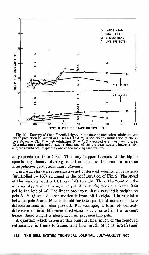
7
6
5
4
3
2
1
=--A A
A
A
t511 LEVELS
35 LEVELS
aa
A
A
A
AA
A
A
C. LARGE HEADX SMALL HEADO MEDIUM HEADA LIVE SUBJECTS
A
A
A
AA
00 0.5 1.0 1.5 2.0 2.5 3.0 3.5 4 0
SPEED IN PELS PER FRAME INTERVAL (PEF)
Fig. 10-Entropy of the differential signal in the moving area when minimum MBElinear prediction is carried out. In each field Pz is the linear combination of the 22pets shown in Fig. 2, which minimizes (Z - Pz)2 averaged over the moving area.Entropies are significantly smaller than any of the previous results ; however, livesubject results are, in general, above the moving area results.
only speeds less than 2 PEF. This may happen because at the higherspeeds, significant blurring is introduced by the camera makinginterpolative predictions more efficient.
Figure 11 shows a representative set of derived weighting coefficients(multiplied by 100) arranged in the configuration of Fig. 2. The speedof the moving head is 0.63 PEF, left to right. Thus, the point on themoving object which is now at pel Z is in the previous frame 0.63pel to the left of M. The linear predictor places very little weight onpels K, N, Q, and V, since motion is from left to right. It interpolatesbetween pels L and M as it should for this speed, but numerous otherdifferentiations are also present. For example, a form of element -difference of field -difference prediction is attempted in the presentframe. Some weight is also placed on previous line pels.
A question which arises at this point is : how much of the removedredundancy is frame -to -frame, and how much of it is intraframe?
1168 THE BELL SYSTEM TECHNICAL JOURNAL, JULY-AUGUST 1975

Thus, some simulations were carried out where the predictor wasonly allowed to use pels from the previous frame in its prediction. Thisis done by deleting in eq. (4) the rows and columns of matrix a andthe elements of column vectors a and ea that correspond to the unusedpels. Entropy results are shown in Fig. 12.
The results are practically the same as in Fig. 10 up to a speed
of about 1.3 PEF which is nearly the range of speeds for which oneshould expect good performance, given the configuration of Fig. 2.
Thus, most of the redundancy removed is frame -to -frame redundancy.Intraframe redundancy becomes important only when the speed is
outside the tracking range of the algorithm.Some simulations were also carried out to test the effect of sub -
sampling at half rate. In this case the predictor is only allowed to usepels B, D, F, G, J, M, P, R, T, U, and V in the prediction. Entropyresults are shown in Fig. 13 for the speed range of 1 to 4 PEF, whichis where subsampling would normally be carried out.
Subsampling increased the entropy as one would expect, but theamount of the increase depended on how much detail there was in themoving area of the scene. With 35 -level quantization, subsamplingincreased the entropies by factors ranging from 1.5 to 2.3 for the largehead, 1.7 to 2.9 for the medium head, and 3.2 to 4.6 for the small head.As the size of the head decreases, the amount of detail increases and,thus, so does the detrimental effect of subsampling. Of course, if theentropy is more than doubled by subsampling, then subsampling athalf rate does not pay.
PRESENT ---..--- .---
---.1m. 6
-12FIELDPELS
..-0..f...
.-- ---II. 2 18
-8
-19 -32 3 011- -..
-12 48 0-2 0 .4....> PREVIOUS.".FRAME
1 -9 5 +/- ---- PE LS
31 9
25 -9!024 -10.4'
-...-...- >PREVIOUS
..---.1 FIELD
PE LS
Fig. 11-A representative set of 22 minimum MSE weighting coefficients multipliedby 100 (see Fig. 2). The mannequin head was moving at 0.63 PEF. Thus, a movingobject point which is at Z in the present frame was 0.63 pels to the left of M in theprevious frame.
FRAME -TO -FRAME CODING 1169
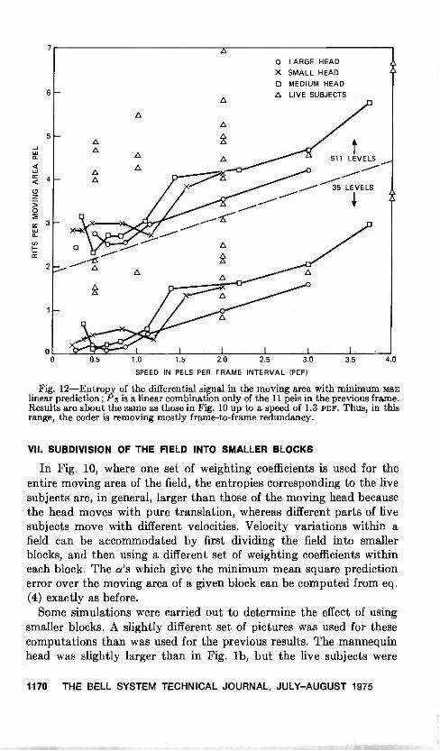
7
6
5
4
3
2
O LARGE HEADX SMALL HEAD0 MEDIUM HEADA LIVE SUBJECTS
A
A
A
A
A
A
A
A
0.5 1.0 1.5 2.0 2.5 3.0
SPEED IN PELS PER FRAME INTERVAL (PEF)
511 LEVELS
35 LEVELS
A
3.5 4 0
Fig. 12-Entropy of the differential signal in the moving area with minimum MBElinear prediction; Pz is a linear combination only of the 11 pels in the previous frame.Results are about the same as those in Fig. 10 up to a speed of 1.3 PEF. Thus, in thisrange, the coder is removing mostly frame -to -frame redundancy.
VII. SUBDIVISION OF THE FIELD INTO SMALLER BLOCKS
In Fig. 10, where one set of weighting coefficients is used for theentire moving area of the field, the entropies corresponding to the livesubjects are, in general, larger than those of the moving head becausethe head moves with pure translation, whereas different parts of livesubjects move with different velocities. Velocity variations within afield can be accommodated by first dividing the field into smallerblocks, and then using a different set of weighting coefficients withineach block. The a's which give the minimum mean square predictionerror over the moving area of a given block can be computed from eq.(4) exactly as before.
Some simulations were carried out to determine the effect of usingsmaller blocks. A slightly different set of pictures was used for thesecomputations than was used for the previous results. The mannequinhead was slightly larger than in Fig. lb, but the live subjects were
1170 THE BELL SYSTEM TECHNICAL JOURNAL, JULY-AUGUST 1975

7
6
5
4
3
2
00 0.5
A
A
A
o LARGE HEADX SMALL HEADO MEDIUM HEADA LIVE SUBJECTS
A
0
A
t511 LEVELS
A
A
35 LEVELS
A
1.0 1.5 2.0 2.5 3.0 3.5 4.0
SPEED IN PELS PER FRAME INTERVAL (PEF)
Fig. 13-Entropy of the differential signal in the moving area with minimum MSElinear prediction with subsampling, i.e., Pz is a linear combination only of pels B,D, F, G, J, M, P, R, T, U, and V.
about the same as in Figs. ld and le. It was found in the simulationsthat the determinant of matrix a in eq. (4) was frequently zero, indi-cating nonunique solutions, i.e., one or more of the a's could be chosenarbitrarily. In this case, the arbitrary a's were set equal to zero and,whenever possible, they were chosen to correspond to pels in thepresent frame.
Figure 14 shows entropies for 511 -level differential signals. Theuppermost curve and its associated live -subject points are obtainedwith no subdivision, as in Fig. 10. The single points are all above themoving -head curve, as before.
The middle curve and points are the entropies which result fromsubdividing the field into 120 blocks (10 horizontal X 12 vertical) andusing a different set of weighting coefficients for each block. Each blockis 21 pels X 10 lines. Not only are the single points closer to the moving -head curve, but all of the points are considerably below those obtainedusing no subdivision. Using smaller blocks, therefore, not only ac -
FRAME -TO -FRAME CODING 1171
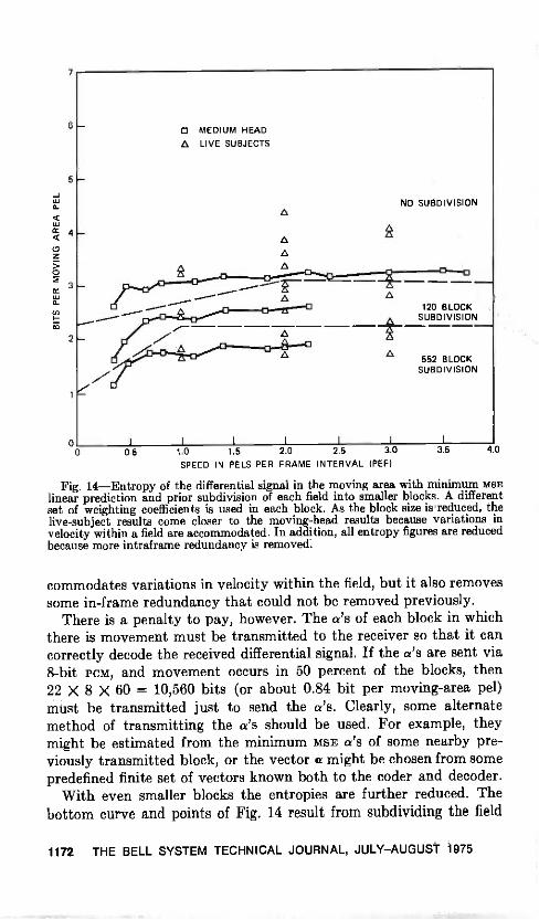
7
6
5
4
3
2
0
MEDIUM HEAD
A LIVE SUBJECTS
A
AAA
A
NO SUBDIVISION
120 BLOCKA SUBDIVISION
A 552 BLOCKSUBDIVISION
0 0.5 1.0 1.5 2.0 2.5 3.0
SPEED IN PE LS PER FRAME INTERVAL (PEF)
3.5 40
Fig. 14-Entropy of the differential signal in the moving area with minimum MSElinear prediction and prior subdivision of each field into smaller blocks. A differentset of weighting coefficients is used in each block. As the block size is reduced, thelive -subject results come closer to the moving -head results because variations invelocity within a field are accommodated. In addition, all entropy figures are reducedbecause more intraframe redundancy is removed.
commodates variations in velocity within the field, but it also removessome in -frame redundancy that could not be removed previously.
There is a penalty to pay, however. The a's of each block in whichthere is movement must be transmitted to the receiver so that it cancorrectly decode the received differential signal. If the a's are sent via8 -bit PCM, and movement occurs in 50 percent of the blocks, then22 X 8 X 60 = 10,560 bits (or about 0.84 bit per moving -area pel)must be transmitted just to send the a's. Clearly, some alternatemethod of transmitting the a's should be used. For example, theymight be estimated from the minimum MSE a's of some nearby pre-viously transmitted block, or the vector a might be chosen from somepredefined finite set of vectors known both to the coder and decoder.
With even smaller blocks the entropies are further reduced. Thebottom curve and points of Fig. 14 result from subdividing the field
1172 THE BELL SYSTEM TECHNICAL JOURNAL, JULY-AUGUST 1975
into 552 blocks (23 horizontal X 24 vertical). Each block is 9 pels X 5lines. Coarse quantization of the differential signal in this case giveszero nearly always. Thus, nearly all of the information about the pelsis carried in the weighting coefficients which, with 50 percent of thearea moving, require 48,576 bits for transmission using 8 -bit PCM. Soif the blocks are made too small, the algorithm is inefficient becauseof the bits required to send the a's.
VIII. CONCLUSION
In a conditional replenishment system for transmitting video -tele-phone pictures, the moving -area picture elements can be coded fortransmission in many ways. Sending frame -to -frame differences andsubsampling at half rate during active movement is simple, reasonablyefficient, and does not fail catastrophically with an occasional trans-mission error. Sending line -to -line differences of frame -differences andsubsampling during active motion is even more efficient and is rea-sonably simple, but it is somewhat less impervious to transmissionerrors.
Adaptive linear predictive coding, which takes into account thespeed and direction of movement in the scene, results in much greatercoding efficiency, indicating that substantial bit -rate savings shouldbe possible. However, system complexity and vulnerability to trans-mission errors are increased accordingly. This means that some kindof error detection -correction scheme is absolutely necessary if adaptivecoding is to be used.
Adaptive coding, which handles speeds of a nonintegral number ofPEFs, performs better than if an integral number of PEFs is assumed.Relatively good results are obtained if for each block in the picture theweighting coefficients are chosen to minimize the mean squared moving -area differential signal. This technique requires transmission in someway of the weighting coefficients so that the decoder can correctlydecode the received differential signal. Thus, if the block size is toosmall, then the system is inefficient because of the number of bitsrequired to send the coefficients. However, even using only one set ofweighting coefficients per field (block size = entire field), significantreductions in differential signal entropies are measured comparedwith nonadaptive coding.
Much work remains to be done before these techniques can be usedin a practical coder. For example, the subjective aspects of interframecoders which track moving objects are as important as the statisticalaspects which are discussed in this paper. Also, many short cuts inimplementation must be developed before these methods are economi-cal. Nevertheless, these results provide a valuable yardstick with which
FRAME -TO -FRAME CODING 1173

simpler and more practical adaptive frame -to -frame coders can becompared.
IX. ACKNOWLEDGMENTS
Much use was made of the picture -processing computer facilityconstructed by R. C. Brainard and J. D. Beyer. Without it these resultswould not have been possible. Also, many fruitful discussions were heldwith D. J. Connor, J. 0. Limb, R. F. W. Pease, and F. W. Mounts.
REFERENCES
1. B. G. Haskell, F. W. Mounts, and J. C. Candy, "Interframe Coding of Video -telephone Pictures," Proceedings of the IEEE, 60, No. 7 (July 1972), pp. 792-800.
2. F. W. Mounts, "Video Encoding with Conditional Picture Element Replenish-ment," B.S.T.J., 48, No. 7 (September 1969), pp. 2545-2554.
3. R. F. W. Pease and J. 0. Limb, "Exchange of Spatial and Temporal Resolutionin Television Coding," B.S.T.J., 50, No. 1 (January 1971), pp. 191-200.
4. J. C. Candy et al., "Transmitting Television as Clusters of Frame -to -FrameDifferences," B.S.T.J., 50, No. 6 (July -August 1971), pp. 1889-1917.
5. J. B. Millard, Y. C. Ching, and D. M. Henderson, private communication.6. D. J. Connor, B. G. Haskell, and F. W. Mounts, "A Frame -to -Frame Picture -
phone® Coder for Signals Containing Differential Quantizing Noise," B.S.T.J.,52, No. 1 (January 1973), pp. 35-51.
7. J. 0. Limb, R. F. W. Pease, and K. A. Walsh, "Combining Intraframe and Frame -to -Frame Coding for Television," B.S.T.J., 58, No. 6 (July -August 1974),pp. 1137-1173.
8. B. G. Haskell, "Buffer and Channel Sharing by Several Interframe Picture -phone® Coders," B.S.T.J., 51, No. 1 (January 1972), pp. 261-289.
9. F. Rocca, "TV Bandwidth Compression Utilizing Frame -to -Frame Correlationand Movement Compensation," Symposium on Picture Bandwidth Compres-sion (M.I.T.), Gordon and Breach, 1972.
10. B. G. Haskell and J. 0. Limb, "Predictive Video Encoding Using MeasuredSubject Velocity," U. S. Patent No. 3,632,865, January 1972.
11. F. K. Manasse, "Directional Correlation-A Technique to Reduce Bandwidthin PCM Television Transmissions," IEEE Transactions on CommunicationTechnology, COM-15, No. 2 (April 1967), pp. 204-208.
12. A. V. Balakrishnan, "An Adaptive Nonlinear Data Predictor," Proc. 1962National Telemetry Conference, 2, Session 6-5.
13. L. D. Davisson, "Theory of Adaptive Data Compression," in Advances in Com-munication Systems, 2, New York: Academic Press, 1966.
14. R. W. Lucky, "Adaptive Redundancy Removal in Data Transmission," B.S.T.J.,47, No. 4 (April 1968), pp. 549-573.
15. F. W. Mounts, private communication.16. D. J. Connor, private communication.17. R. F. W. Pease, private communication.18. R. F. W. Pease, "Conditional Vertical Subsampling-A Technique to Assist
in the Coding of Television Signals," B.S.T.J., 51, No. 4 (April 1972), pp.787-802.
1174 THE BELL SYSTEM TECHNICAL JOURNAL, JULY -AUGUST 1975

Contributors to This Issue
James E. Bennett, B.Sc. (Met. E.), 1959, Carnegie Institute ofTechnology; M.Sc. (Metallurgy), 1961, and Ph.D. (Metallurgy), 1965,Case Institute of Technology; General Electric Refractory MetalsLaboratory, 1964-1966 ; Battelle Memorial Institute, 1966-1968 ; BellLaboratories, 1968-. At the Columbus Laboratories, Mr. Bennett hasbeen conducting fundamental studies on the interaction of liquidmercury with contact metals, interdiffusion in connector materials,phase transformations in and processing behavior of Fe/Co/2-3% Valloys, and contact materials development. Member, AIME, IMS,Alpha Sigma Mu, Sigma Xi.
Dan Bisbee, B.S., 1965, Monmouth College; Bell Laboratories,1955-. Mr. Bisbee has worked on the design and measurement ofmillimeter waveguide components. He has also been involved with thestudy and measurement of transmission losses in bulk glass and optical -fiber waveguides. He is presently engaged in developing techniques forsplicing optical fibers and cables.
Edwin L. Chinnock, Stevens Institute of Technology; Bell Labora-tories, 1939-. Mr. Chinnock has worked on microwave components,microwave radio relay, and helix waveguide fabrication. He is presentlyworking on optical waveguide components.
Leonard J. Forys, B.S.E.E., 1963, University of Notre Dame; M.S.and E.E., 1965, Massachusetts Institute of Technology; Ph.D., 1968,University of California at Berkeley; Acting Assistant Professor ofElectrical Engineering, University of California at Berkeley, 1967-1968; Bell Laboratories, 1968-. Upon joining Bell Laboratories, Mr.Forys was engaged in research and consulting on communication andcontrol theory problems. He later was involved in studies of the anal-ysis and control of an air traffic system and worked on the real-timeprediction of demands for a domestic satellite system. He is currentlysupervisor of the Traffic Studies Group doing capacity studies of elec-tronic switching machines.
D. Gloge, Dipl. Ing., 1961, Dr. Ing., 1964, Technical Universityof Braunschweig, Germany ; Bell Laboratories, 1965-. Mr. Gloge'swork has included the design and field testing of various optical trans -
1175

mission media and the application of ultra -fast measuring techniquesto optical component studies. He is presently engaged in transmissionresearch related to optical -fiber communication systems.
Barry G. Haskell, B.S., 1964, M.S., 1965, and Ph.D. (ElectricalEngineering), 1968, University of California, Berkeley; ResearchAssistant, University of California, 1965-1968; Bell Laboratories,1968-. Mr. Haskell is a member of the Visual Communication Re-search Department. His primary interest is the efficient coding ofpictures for transmission at reduced bit rate. Member, Phi Beta Kappa,Sigma Xi, IEEE.
Sing-Hslung Lin, B.S.E.E., 1963, National Taiwan University;M.S.E.E., 1966, and Ph.D., 1969, University of California, Berkeley;Bell Laboratories, 1969-. At the Electronics Research Laboratory,University of California at Berkeley, Mr. Lin was engaged in researchon antennas in plasma media and numerical solutions of antenna prob-lems. Mr. Lin is presently working on wave propagation problems onterrestrial radio systems and earth -satellite radio systems. Member,IEEE, Sigma Xi, AIAA.
Dietrich Marcuse, Diplom Vorpruefung, 1952, Dipl. Phys., 1954,Berlin Free University; D.E.E., 1962, Technische Hochschule, Karls-ruhe, Germany ; Siemens and Halske (Germany), 1954-1957 ; BellLaboratories, 1957-. At Siemens and Halske, Mr. Marcuse was en-gaged in transmission research and studying coaxial cable and circularwaveguide transmission. At Bell Laboratories, he has been engaged instudies of circular electric waveguides and work on gaseous masers. Hespent one year (1966-1967) on leave of absence from Bell Laboratoriesat the University of Utah. He is presently working on the transmissionaspect of a light communications system. Mr. Marcuse is the author ofthree books. Fellow, IEEE; member, Optical Society of America.
J. E. Mazo, B.S. (Physics), 1958, Massachusetts Institute of Tech-nology; M.S. (Physics), 1960, and Ph.D. (Physics), 1963, SyracuseUniversity; Research Associate, Department of Physics, University ofIndiana, 1963-1964; Bell Laboratories, 1964-. At the University ofIndiana, Mr. Mazo worked on studies of scattering theory. At BellLaboratories, he has been concerned with problems in data transmis-sion and is now working in the Mathematical Research Center.Member, American Physical Society, IEEE.
1176 THE BELL SYSTEM TECHNICAL JOURNAL, JULY -AUGUST 1975
E. J. Messerli, B.A.Sc. (E.E.) 1965, University of British Columbia;M.S. (E.E.) 1966, University of California at Berkeley; Ph.D. (E.E.and Comp. Sc.) 1968, University of California at Berkeley; ActingAssistant Professor of Electrical Engineering, University of Californiaat Berkeley, 1968-1969 ; Bell Laboratories, 1969-. Mr. Messerli hasbeen involved in studies on the analysis and control of an air trafficsystem and on the demand assignment of capacity for a domesticsatellite system. He has also worked on the development of optimiza-tion algorithms. Since 1971, his work has been concerned with tele-phone traffic analysis and modeling. Currently, his work is concernedwith the effect of measurement and forecasting errors on the trunkprovisioning process.
M. Robert Pinnel, B.Sc. (E.E.), 1966, M.Sc. (Met.E.), 1968, andPh.D. (Materials Sci.), 1970, Drexel University; Bell Laboratories,1970-. Mr. Pinnel has been engaged in research on the characterizationof the physical and mechanical behavior of numerous copper -basedalloys used as spring materials, interdiffusion in electrical connectormaterials, the detailed characterization of the Fe/Co/2-3% V alloysystem, and the interaction of liquid mercury with numerous metallicelements. His current interests are in the areas of magnetic materialsand solid-state diffusion. Member, ASM, AIME, Tau Beta Pi, PhiKappa Phi, Alpha Sigma Mu, Eta Kappa Nu.
Vasant K. Prabhu, B.E. (Dist.), 1962, Indian Institute of Science,Bangalore, India; S.M., 1963, Sc.D., 1966, Massachusetts Instituteof Technology; Bell Laboratories, 1966-. Mr. Prabhu has been con-cerned with various theoretical problems in solid-state microwavedevices, noise, and optical communication systems. Member, IEEE,Eta Kappa Nu, Sigma Xi, Tau Beta Pi, and Commission 6 of URSI.
Harrison E. Rowe, B.S., 1948, ALS., 1950, and Sc.D., 1952, Massa-chusetts Institute of Technology; Bell Laboratories, 1952-. Mr.Rowe's fields of interest have included parametric amplifier theory,noise and communication theory, modulation theory, propagation inrandom media, and related problems in waveguide, radio, and opticalsystems. Fellow, IEEE; member, Sigma Xi, Tau Beta Pi, Eta KappaNu, and Commission 6 of URSI.
Adel A. M. Saleh, B.Sc. (Electrical Engineering), 1963, Universityof Alexandria, Alexandria, Egypt; S.M., 1967, Ph.D. (Electrical
CONTRIBUTORS TO THIS ISSUE 1177

Engineering), 1970, Massachusetts Institute of Technology ; Universityof Alexandria, 1963-1965, Instructor and Demonstrator; Bell Labora-tories, 1970-. Mr. Saleh is engaged in studies of millimeter -wavecomponents, devices, and propagation. Member, Sigma Xi, IEEE.
Peter W. Smith, B.Sc., Mathematics and Physics, 1958, and M.Sc.and Ph.D., Physics, 1961 and 1964, McGill University; VisitingMackay Lecturer in Electrical Engineering, 1970, University ofCalifornia, Berkeley; Bell Laboratories, 1964-. Mr. Smith has in-vestigated a number of systems for obtaining single -frequency laseroperation and is currently investigating the use of waveguide tech-niques for producing miniature gas lasers. Member, American PhysicalSociety, Optical Society of America, IEEE.
Richard H. Turrin, B.S.E.E., 1956, Newark College of Engineering;M.S.E.E., 1960, New York University; Bell Laboratories, 1956-.Mr. Turrin has been concerned with propagation and antenna workat micro- and millimeter wavelengths. He participated in the designof the Telstar® satellite ground -station antennas and is presentlyengaged in studies of satellite antennas. Member, IEEE, Eta KappaNu, Tau Beta Pi.
1178 THE BELL SYSTEM TECHNICAL JOURNAL, JULY -AUGUST 1975