The Australian National University

Centre for Economic Policy Research

DISCUSSION PAPER

What's love got to do with it? Homogamy and dyadic approaches to understanding marital instability

Rebecca Kippen, Bruce Chapman, Peng Yu

DISCUSSION PAPER NO. DP631

January 2010

ISSN: 1442-8636 ISBN: 978-1-921693-12-0

Dr Rebecca Kippen, Australian Demographic and Social Research Institute, The Australian National University Ph: +61 2 6125 3759, Fax: +61 2 6125 2992, Email: rebecca.kippen@anu.edu.au Professor Bruce Chapman, Crawford School of Economics and Government, The Australian National University Dr Peng Yu, Department of Families, Housing, Community Services and Indigenous Affairs

ii

Abstract

The determinants of marital instability is an important area of research for demography,

sociology and economics, with a host of public policy outcomes being significantly affected

by family breakdown. This paper improves our understanding of the issue through the use of

rich longitudinal data and the application of advanced research approaches. In both method

and data terms our approach represents a significant advance in this research area.

Using data from waves 1–7 of HILDA, 2,482 married couples—where both partners are

respondents in the first wave—are traced over six years to identify factors associated with

marital instability. The data are analysed dyadically; that is, the characteristics of both

partners in each couple are considered in tandem. This allows assessment of whether

marriages between partners with similar characteristics (homogamy) are more likely to last

than are marriages between dissimilar partners, or whether particular characteristics of wives

or husbands—independent of their partners’—are more strongly associated with marital

stability. A Cox proportional hazards model with time-varying covariates is used to assess the

association of characteristics with marital separation.

We find the following factors are associated with higher risk of marital separation: spousal

differences in age, education, preference for a(nother) child, and drinking and smoking

behaviours; dissatisfaction with the relationship; low household income; husband’s

unemployment and perceived financial stress; young age at marriage; separation of parents;

second-plus marriage; and resident children born before marriage.

JEL Codes: J10; J12; R20 Keywords: marriage, marital separation, divorce, Australia, dyadic, homogamy.

1

Introduction Based on 2000–2002 marriage and divorce rates, 72 per cent of the Australian population will legally marry at some point in their lives; of these marriages, one-third are expected to end in divorce (Jain 2007) and others will end in permanent separation without the formality of divorce (Hewitt, Baxter and Western 2005). Marital breakdown is experienced by a significant proportion of the Australian population. The apparent economic and social consequences of marital breakdown are well documented. Divorced people have lower levels of general wellbeing (Amato 2000), lower rates of home ownership and less wealth in later life than do the married (de Vaus et al. 2007). Children of divorced parents have lower scores on indicators of behaviour, psychological adjustment, scholastic success, social interactions and self-concept than do children of continuously married parents (Amato 2001). The economic cost of divorce to the Australian community is large: direct costs were estimated at three billion dollars per annum in the mid-1990s (HOR 2008). The financial costs to mothers and their children are considerable as well (Gray and Chapman 2007). Using data from the first seven waves of the Household, Income and Labour Dynamics in Australia Survey (HILDA), this study adds to previous Australian and international research on the correlates of marital dissolution by investigating individual and couple characteristics associated with marital instability. Critically, and for the first time in combination, we employ sophisticated econometric methods (time-varying covariates), longitudinal data and dyadic information (information concerning both individuals in the marriage). The paper begins with a review of relevant literature and theory, after which the data and method are described, followed by discussion of the results. Theory: Becker’s model of marital utility This study takes its cue from the seminal work by Becker, Landes and Michael (1977), which states that the only circumstance under which a marriage will dissolve is if the joint marital utility is less than the joint utility of ending the marriage. Thus marriages of homogamous couples are likely to be more stable than those of couples with dissimilar characteristics, since like traits such as religion and age are complementary and tend to maximise gain from the marriage (Becker 1973). Homogamous attributes considered in this research include country of birth, age, preference for a child or another child, religiosity, education, and drinking and smoking behaviours. According to Becker et al. (1977), exceptions to the homogamy hypothesis are traits associated with the division of labour within marriage. All else being equal, spouses who assume distinct marital roles—such as wage earner and child rearer—have lower marital dissolution rates than do couples with less differentiated duties, since specialisation means greater gain from remaining married (Becker et al. 1977). An extension of this is the ‘independence hypothesis’; that women with higher human capital in terms of market productivity are more likely to divorce, because their marital utility is lower than that of wives in traditional breadwinner-model marriages. They have the means and resources to leave a marriage (Chan and Halpin 2003). In this framework, rising divorce rates over the twentieth century are considered to have resulted—in part—from rising female labour force participation rates (Jalovaara 2003). Others argue that the specialisation model

2

and independence hypothesis are becoming increasingly irrelevant as gender roles continue to blur (Lyngstad 2004). Although the focus of this paper is the association between marital homogamy and marital stability, we also test the independence hypothesis by considering the impact of wives’ economic-utility characteristics controlling for their husbands’ characteristics. The expected effect is not always clear. For example, for some given distribution of marital duties, more-educated couples will have higher utility on average than will less-educated couples, decreasing their risk of union dissolution. However more-educated couples are also less likely to specialise (that is, assume traditional gender roles), increasing the probability of dissolution (Becker et al. 1977). Additionally, educated wives are more likely to have the resources required to survive post-married life, which reduces their marital utility relative to the utility of becoming single. Under the independence hypothesis, more highly educated women, women who are employed, or women with a strong work history would be associated with higher marital separation rates than other women. The sections below discuss characteristics of husbands and wives—individually and dyadically—that have been found to be associated with marital instability. Empirical results from the literature

There is a considerable empirical literature concerned with the determinants of marital (in)stability. However, while there is agreement about the essential questions this is not the case with respect to research methods, data and statistical approach. Even so, it is possible to document areas of some agreement with respect to results, and these factors can be categorised as ‘Homogamous’, ‘Satisfaction’, ‘Socio-economic’ and ‘Marriage and children’ variables. Homogamous variables Ethnicity. A number of studies have found an association between differing ethnicities and risk of marital dissolution. Becker et al. (1977) hypothesise that interracial marriages are at greater risk than are same-race unions due to lower marital utility. Research in the United States supports this hypothesis (Bratter and King 2008; Bumpass, Martin and Sweet 1991; Lehrer 2008). Partners of differing ethnicities are more likely to have dissimilar cultural backgrounds and views of marriage (Bratter and King 2008; Hewitt 2008; Lehrer 2008) and may encounter disapproval of their relationship (Bratter and King 2008), leading to reduced gains from marriage. In addition, if one or more partners have migrated, this may add to marital stress (Hewitt 2008). Age difference. Many studies show that disparities in age between husband and wife are associated with higher rates of divorce. This is especially true if a man is significantly younger than his wife (Chan and Halpin 2003; Lehrer 2008; Teachman 2002). This may be due to differences in values associated with birth cohort, or marital strain caused by power imbalances within the union (Bumpass and Sweet 1970). Preferences for more children. According to the homogamy hypothesis, partners with the same desires for future children should have stronger unions than couples with dissonant

3

fertility preferences. Research findings have been mixed. A longitudinal U.S. study found that marriages were more likely to end if the wife wanted fewer children than her husband (Coombs and Zumeta 1970). Clarkwest (2007) concluded that differences between spouses in desired number of children is correlated with a higher risk of marital dissolution. However Thomson (1997) found that a couple’s childbearing intentions or desires are not associated with union breakdown. Religion and religiosity. If homogamous marriages are more stable, then couples with shared religious beliefs—or shared lack of religious beliefs—and similar levels of religiosity would be expected to have a lower risk of separation than couples with different religions and levels of religiosity. However this effect might be confounded through the influence of religion itself. Many religions’ teachings on the sanctity of marriage and primacy of the family unit may mean that the religiosity of one spouse has a protective effect on the marriage through increased psychological costs of union dissolution, irrespective of the beliefs of the other partner (Lehrer 2004). Education. The expected effect of education on the risk of marital dissolution depends on which theory is applied. Under the homogamy hypothesis, couples with similar levels of education have increased value consensus, leading to raised marital utility and lower separation rates. However more-educated couples are likely to have less-defined marital roles, increasing the probability of marriage breakdown (Becker et al. 1977). Under the independence hypothesis, educated women are more likely to have the resources required to survive post-married life, increasing the gain of becoming single relative to the gain of remaining married. Some studies conclude that educational homogamy is correlated with marital stability (Jalovaara 2003; Tzeng 1992; Weiss and Willis 1997). Others find no such effect (Chan and Halpin 2003; Lyngstad 2004). Recent Australian research reported that educationally heterogamous marriages were at greater risk of dissolution, particularly those in which the wife was much more highly educated than her husband (Butterworth et al. 2008). Alcohol consumption. Applying the homogamy hypothesis, couples with similar drinking patterns should be less likely to end their marriage than couples with disparate levels of alcohol consumption. This is in fact what some research has found: unions are more stable if husband and wife have concordant drinking patterns (Homish and Leonard 2007; Ostermann et al. 2005). Ostermann et al. (2005) outline three ways in which high alcohol consumption by either partner could raise the risk of marital dissolution. The first is that sustained heavy drinking during the search for a spouse could lead to a suboptimal match. Heavy drinkers are more likely to marry young, suggesting a shorter search time for a mate. They may also be viewed as inferior potential partners because of their high alcohol consumption, and associated problems such as poor health; Second, alcohol abuse may hinder fulfillment of the agreed marital role—including basic domestic tasks or participation in the workforce—leading to decreased marital utility and a higher probability of separation. Finally, the spouse of a heavy drinker may anticipate that the drinking will reduce or stop at some point. If this does not occur, the perceived gain from ending the marriage may increase (Ostermann et al. 2005).

4

In their study of middle-aged Americans, Ostermann et al. (2005) found that heavy drinking by one or both partners was associated with marital breakdown. However other research concludes that high alcohol consumption is linked to increased risk of union dissolution (Caces 1999; Power and Estaugh 1990). Smoking. Similar to the homogamy argument for alcohol consumption, couples who either both smoke or both do not smoke should be at less risk of separation than couples in which one partner smokes and the other does not, all else being equal. However Butterworth et al. (2008) find that smoking by one or both spouses is associated with higher probability of marital breakdown. They conclude that individuals who smoke are more likely to be socially and economically disadvantaged, and these people are at greater risk of marital instability. A study based on the U.S. National Longitudinal Survey of Youth (Fu and Goldman 2000) found an elevated risk of marital dissolution for smokers, but were unable to test the impact of concordant smoking behaviour in a couple. Using the same dataset, Compton (2009) argues that couples in which one or both partners ‘heavily discount the future’ are more likely to indulge in risky practices such as smoking, and are also more likely to end a marriage. Thus the association between smoking and marital dissolution works through the relationship of both to an individual’s rate of time preference. Satisfaction variables Satisfaction with life/satisfaction with relationship. Clearly, couples who rate their relationship highly are more likely to have a stable union than couples who are unhappy with their marriage. In the mid-1970s, Ross and Sawhill (1975) hypothesised that as divorce became more normative and, as the traditional demarcation of marital roles became more relaxed, couples in unsatisfying marriages would be more likely to end their relationship. This would mean a lower proportion of marriages succeeding, but those that did would in general be more satisfying than those in the past. Research in the Western world consistently shows that marital separation is more often initiated by the wife than by the husband (Hewitt et al. 2006; Kalmijn and Poortman 2006; Smith 1997; Zeiss et al. 1981). Given this, it might be expected that a wife’s satisfaction with the marital relationship, and with life in general, would be a more significant determinant of marital stability than is her husband’s satisfaction. Socio-economic variables Employment status. Previous research in Australia indicated that the relationship between women’s employment and marital instability had attenuated over time (Bracher et al. 1993), and a recent study found no correlation (Butterworth et al. 2008). This lends credence to the argument that the independence hypothesis is less relevant in an era where most women work outside the home (Lyngstad 2004). However research in Australia (Bracher et al. 1993; Butterworth et al. 2008) and internationally (Hansen 2005; Jalovaara 2003; Jensen and Smith 1990; Kiernan and Mueller 1999) consistently finds strong effects for unemployment, particularly male unemployment, on the risk of marital dissolution.

5

Financial status. Economic hardship can increase personal stress levels, leading to strained marital relations (Bradbury and Norris; Wolcott and Hughes 1999). In addition, reduced financial resources within the marriage may raise the relative utility of ending the relationship. Research findings have been mixed. Some studies have found that household income is inversely associated with the risk of union dissolution (Chan and Halpin 2003; Jalovaara 2003) while others find no correlation (Jensen and Smith 1990). Marriage and children variables Separation/divorce of parents. A strong predictor of marital dissolution is separation or divorce of the parents of either husband or wife, or both (Amato 1996; Bratter and King 2008; Bumpass et al.; Butterworth et al. 2008; Hewitt et al. 2005; Wolfinger 2003). Amato (1996) concludes that intergenerational transmission of divorce occurs because children of divorced parents are more likely to see marital dissolution as normative, and are more likely to have interpersonal styles that are not conducive to marital harmony. Butterworth et al. (2008) and Bumpass et al. (1991) find that the association between parental divorce and marital instability is stronger where the marriage of the husband’s parents failed, while Amato (1996) found the risk of marital dissolution was higher when wives’ parents had divorced. Marital duration. In general, the length of a marriage is inversely related to its likelihood of dissolution. This is partly due to heterogeneity in the married population; those most likely to separate tend to do so early. In addition, accumulation of marital-specific capital—including children, spousal compatibility and familiarity—increases marital utility over time (Becker et al. 1977; Bracher et al. 1993). Age at marriage. Early age at marriage is found to be correlated with an increased risk of marital instability (Becker et al. 1977; Chan and Halpin 2008; Lehrer 2008). Young newly-weds will likely have spent a shorter period on the marriage market than older people, and will have less idea of what constitutes an optimal match, increasing the probability of low marital gain and, hence, union dissolution (Becker et al. 1977). Young people are also more likely to be lacking the interpersonal skills and economic resources associated with marital success (Hewitt 2008). However marriage at ages beyond the norm may also be associated with higher rates of dissolution. Similar to the reasoning above for marriage order, those marrying at older ages have less choice on the marriage market, and may enter sub-optimal relationships. Women especially may choose to reduce their expectations of a partnership so as to marry before reaching the end of their reproductive years (Becker et al. 1977). Marriage order. Second and higher-order marriages—where the previous marriage or marriages ended in divorce—are known to be less stable in general than first marriages. Poortman (2007), following Becker et al. (1977), posits four main reasons for this. The first is that people in second-plus unions are selected on the basis that their former marriage did not last, and are thus more likely to have personal characteristics that increase the risk of marital separation. Secondly, children and other connections to previous unions may increase conflict in the current relationship. Third, the marriage market will probably be smaller second time around, making it less likely that a good match will be found. Finally, the experience of marital breakdown may result in greater caution and lower levels of commitment in a subsequent marriage. Cohabitation. The overwhelming bulk of research on cohabitation and marital instability finds that cohabitation before marriage is linked to a greater probability that the marriage will fail

6

(Amato 1996; Hohmann-Marriott 2006; Teachman 2002; Wagner and Weiss 2006). This is in line with prior Australian research (Bracher et al. 1993; Butterworth et al. 2008; Hewitt, Baxter and Western 2005). De Vaus et al. (2003) consider three possible reasons for this relationship. The first is that the process of cohabitation can cause or strengthen convictions that marriage is not inviolate, leading to an increased propensity to end a marriage once it is contracted. Second, the link between cohabitation and divorce may work through individual characteristics; people with certain combinations of traits are both more likely to enter de facto relationships, and to divorce, independent of whether or not they cohabited before tying the knot. Third, comparing dissolution rates by length of marriage may lead to overestimation for marriages preceded by cohabitation, since these unions extend back before the beginning of formal marriage. In this case, comparing dissolution rates by living-together duration may give more accurate results. De Vaus et al. (2003) posit that if the second reason above is correct, then its effect should decrease as the proportion of the population who live together before marriage increases. This is because people who form de facto relationships are less and less likely to have personal characteristics associated with marital instability. In support of this hypothesis, de Vaus et al. (2003) find that—with and without a control for living-together duration—the difference in marital separations between couples who cohabited before marriage and those who did not, is statistically insignificant for recent marriage cohorts. Children before the marriage. As noted in the discussion above on marriage order, children from previous unions may bring about conflict in subsequent marriages, resulting in reduced probability that the marriage will be maintained. Similarly, children from a current union, but born before marriage, may be associated with increased risk of marital dissolution if birth prompted a marriage that otherwise would not have occurred (Hewitt 2008). Number and age of resident children. According to Becker et al. (1977), all else being equal, couples with young children have more stable marriages than do couples without children, since children are ‘marital-specific capital’. An Australian study found that resident children aged five years and under decreased the probability of marital dissolution. The study concluded that this may be because wives—as primary care givers—are more dependent on their partners when young children are present, and thus will be less likely to terminate the union. Alternatively, couples who would otherwise separate may choose to remain together for the sake of the children (Bracher et al. 1993). Recent research from the United Kingdom finds that there the effect of children has been reversed; the presence of children, especially two or more children, raises the risk of divorce for recent marriage cohorts. The authors speculate that attitudes towards children may have changed; fathers may now be more likely to shirk their paternal responsibilities; or the norming of divorce may mean that recent cohorts see ending a marriage as an acceptable response to the stress of parenthood. Finally, the authors conclude that they ‘are more inclined to seek the answer in changes in the timing of fertility in interaction with the changing timing and nature of partnership, than in profound changes in the moral disposition of the British population’ (Chan and Halpin 2003).

7

Are there stylised facts? From the myriad of different research, using dissimilar data and methods, several findings appear to be shared. These include that the probability of marital separation is negatively associated with: marriage duration, age at marriage, parental divorce, the overall level of education of the couple, and husband’s experiencing unemployment. There is little to report that is consistent with respect to homogamy, measured in various ways. Data The data used in this study are from the Household, Income and Labour Dynamics in Australia Survey (HILDA), a household-based representative longitudinal survey that currently has available seven annual waves for the period 2001–2007. Wave 1 sampled 7,682 households. The sample for this study is limited to the 2,482 couples who were legally married, co-resident, 58 years or less, and both interviewed in the first wave of HILDA. These couples are traced over the subsequent six waves to determine which remained together, and which divorced or separated. The number of male and female respondents by characteristics in our wave 1 sample, and the proportion who had separated by wave 7, are shown in Table 1. For characteristics of the marriage—such as marital duration and number and age of co-resident children—results are shown in the ‘Females’ column. Where different marriage characteristics were reported by husband and wife, the wife’s responses are reported. In total, 10.7 per cent of couples had separated by wave 7 of the survey. Table 2 shows the breakdown of the dyadic variables used in the analysis, with characteristics of husbands and wives considered in tandem. Again, the number of cases in wave 1, and the percentage separated by wave 7 are given. Below is a list of the data in Tables 1 and 2. Current age. Calculated from date of birth and date of wave 1 survey. Age at the time of the survey does not enter our analysis, since we account for both age at marriage and length of marriage. However, from the descriptive data, there appears to be a strong inverse relationship between age at wave 1 and subsequent marital breakdown.

Education (‘Looking at SHOWCARD C7a, what qualifications have you completed?’). Data are grouped as ‘Bachelor degree or above’, ‘Other post-school qualification’, ‘Completed high school’, and ‘Did not complete high school’.

Equivalised household income. This is a derived variable based on annual income of household residents from all sources, adjusted by the Consumer Price Index to 2001 dollars (ABS 2009), and adjusted for number of household residents using the Australian Bureau of Statistics’ equivalence scale (ABS 2006).

Employment status. Data for this variable are categorised as ‘Works 0–34 hours per week’ (part time), ‘Works 35 or more hours per week’ (full time), ‘Unemployed’ and ‘Not in the labour force’.

Years in paid employment (‘Now of these years/months [since you left full-time education for the first time], how many years/months in total have you spent…in paid work?’).

8

Length of marriage. This variable is calculated from date of marriage (‘In what month and year were you married?’) and date of wave 1.

Age at marriage. Calculated from date of birth and date of marriage.

Lived together before this marriage (‘Some people live together before marrying, did you and your wife/husband live together before marrying?’).

Children before this marriage. Calculated from dates of birth of resident children and date of marriage.

Number of resident children. Calculated from natural, adopted, step, and foster children who usually reside in the household.

Age of youngest resident child. Calculated from dates of birth of natural, adopted, step, and foster children who usually reside in the household.

Like to have a(nother) child (Would you like to have [a child of your own /more children] in the future?:.. Pick a number between 0 and 10… The more definite you are that you would like to have [a child/more children], the higher the number you should pick. The more definite you are that you do not want to have [a child/more children], the lower the number’).

Country of birth (‘In which country were you born?’). HILDA does not record ethnicity or race, so we use country of birth to proxy ethnicity and culture.

Age difference. Calculated from spousal dates of birth.

Difference in preference for a(nother) child (Would you like to have [a child of your own /more children] in the future?:.. Pick a number between 0 and 10…’). This variable is categorised as ‘Husband and wife have similar preference’ (same or one point difference), ‘Wife moderately stronger preference’ (wife 2–4 points higher), ‘Wife much stronger preference’ (wife 5–10 points higher), ‘Husband moderately stronger preference’ (husband 2–4 points higher), and ‘Husband much stronger preference’ (husband 5–10 points higher).

Religiosity (‘On a scale from 0 to 10, how important is religion in your life?’).

Difference in education. Using the four education categories from Table 1, spouses were classified as having the same level of education if they fell into the same category. Husband’s education was much higher if the wife did not complete high school and the husband had a post-school qualification or a bachelor degree or above, or if the wife completed high school and the husband had a bachelor degree or above. Husband was higher if the wife did not complete high school and the husband completed high school, or the wife completed high school and the husband had other post-school qualification, or the wife had other post-school qualification and the husband had a bachelor degree or above. Similar logic was used to classify into ‘Husband lower’ and ‘Husband much lower’.

Standard drinks per day (‘On a day that you have an alcoholic drink, how many standard drinks do you usually have? 13 or more / 9 to 12 / 7 to 8 / 5 to 6 / 3 to 4 / 1 to 2’. Skipped for ‘I have never drunk alcohol’ and ‘I no longer drink’ which were classified as 0).

Smoking (‘Do you smoke cigarettes or any other tobacco products? No, I have never smoked / No, I have given up smoking / Yes’).

Satisfaction with life (‘All things considered, how satisfied are you with your life?: ..Pick a number between 0 and 10 to indicate how satisfied you are.’).

Satisfaction with relationship (‘How satisfied are you with your relationship with your partner?’).

9

Perceived prosperity (‘Given your current needs and financial responsibilities, would you say that you and your family are…Prosperous / Very comfortable / Reasonably comfortable / Just getting by / Poor / Very poor’). ‘Prosperous’, ‘Very comfortable’ and ‘Reasonably comfortable’ are classified as ‘Comfortable to prosperous’; ‘Just getting by’, ‘Poor’ and ‘Very poor’ classed as ‘Very poor to just getting by’.

Parents ever separated/divorced (‘Did your mother and father ever get divorced or separate?’).

Marriage order (‘How many times, in total, have you been legally married?’). Method Divorce or separation was considered to have occurred if at least one partner was interviewed in a wave subsequent to wave 1 and reported their marital status as either separated or divorced. Couples were censored at the date (month and year) of separation/divorce. Couples in which neither partner was interviewed in subsequent waves were right censored at last wave of interview. The death of a spouse also led to right censoring. All couples still married at wave 7 were right-censored at that point. We recognise that our results may be affected by attrition bias if couples who separated were more likely to leave the survey than those couples who stayed together. Separation usually causes a residential shift for one or both partners, which may mean that respondents cannot be located in survey waves subsequent to their separation, and thus their separation is not recorded. This bias, if it exists, would tend to weaken our conclusions, since the inclusion of these cases would increase explanatory power of the model. Cox proportional hazards model was used to measure the hazard of marriages—observed in wave 1 of HILDA—ending in separation or divorce by wave 7. The Cox hazard function takes the form:

ii xthth exp0 [1]

where hi(t) is the hazard of separation/divorce occurring at marriage duration t for the ith couple; xi is the set of covariates specific to the ith couple; is the set of coefficients estimated to fit the Cox model; and h0(t) is the baseline hazard function—the hazard function resulting from covariate values all set to zero (Cox 1972; DeMaris 2004). One advantage of the Cox model is that the functional form of the hazard over time t does not have to be defined. Dividing both sides of equation [1] by h0(t) gives:

ii xth

thexp

0

[2]

where th

thi

0

is the ratio of the separation hazard of the ith couple relative to the baseline

hazard. The hazard ratio is assumed to be constant over marital duration t, with the hazard for couple i equal to ixexp multiplied by the (undefined) baseline hazard. That is, any two

10

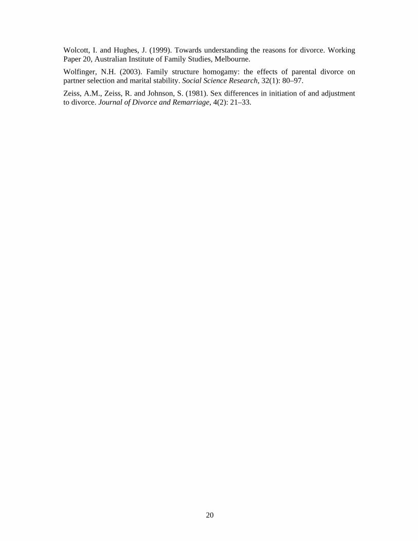
hazards are proportional over time (Cox 1972; DeMaris 2004). We verified the proportional hazards assumption by analysing the Schoenfeld residuals (Cleves et al. 2004). In using the Cox model, we set time t equal to marriage duration, since the risk of separation varies over the life of a marriage. Our observation begins at wave 1 of couples who are already married. This means, in all cases, there is some unobserved duration between the commencement of marriage (t=0) and wave 1 of HILDA. The Cox model deals with this through left truncation or delayed entry, recognising that couples were at risk of separation for some known, but unobserved, period before the survey, and that entry to observation is conditional on the marriage having survived to the point of observation (DeMaris 2004). The Cox model allows for time-varying covariates; that is, independent variables that change over the period of observation—such as number and age of children—can be altered in the model at the point t of change. In this research we use this feature to update marital characteristics at each survey wave in the analysis. A number of previous studies have used HILDA data to consider correlates of marital instability. De Vaus et al. (2003; 2005), Hewitt et al. (2005; 2006), Hewitt (2008) and Hewitt and de Vaus (2009) based their research on marital histories of respondents collected in the first wave of HILDA, and so were able to examine characteristics of one partner associated with union dissolution. Bradbury and Norris (2005), Butterworth et al. (2008) and Butterworth and Rodgers (2008) tracked couples in wave 1 of HILDA over succeeding waves to determine individual and couple characteristics at wave 1 that were correlated with subsequent marital breakdown. To our knowledge, this is the first marital-dissolution study based on HILDA that uses Cox regression and time-varying covariates updated for each observed survey wave. This allows us to consider the impact of potentially impermanent characteristics (such as education and religiosity) as immediate factors associated with marital instability. Results Figure 1 shows the Kaplan-Meier marriage survival curve, a non-parametric estimate of the probability that a married couple has not experienced separation by marital duration t, based on unweighted HILDA data:

t

j j

jj

n

dntS

0

[3]

where jn is the number of couples at risk of separation at marriage duration j and jd is the

number of separations at duration j. This can be regarded as a cross-sectional, or period, measure of the cumulative risk of separation. That is, the figure shows a survival curve for a hypothetical marriage cohort based on duration-specific marital separation probabilities observed over the period 2001–2007. It shows that about 25 per cent of couples can expect to experience separation by marriage duration 6 years, and 50 per cent by duration 26 years. Figure 2 shows the monthly hazard of separation associated with Kaplan-Meier survival curve. Separation risk peaks at marital duration five years, and declines steadily after 20 years. Since under the Cox model any two hazards are proportional over time (time in this

11

case being defined as marital duration), a shift in population characteristics will move this curve up or down but not change its basic shape. Cox model results are shown in Table 3. The ‘Hazard ratio’ is the impact on the probability of marital separation of the given category relative to the reference category, controlling for all other variables. For example, a hazard ratio of 1.90 means that the probability of separation for the given category is 90 per cent higher than for the reference category. A hazard ratio of 0.65 means the probability of separation for the given category is 35 per cent less than for the reference category. The ‘p-value’ column gives the probability of a Type-I error: what is the probability of the sample yielding the observed separation hazard ratio, if the given category and the reference category actually had the same separation hazard in the population from which the sample was drawn? In this paper, p-values of less than 0.05 are heavily shaded and p-values between 0.05 and 0.10 are lightly shaded. Model 1 analyses all the variables previously outlined. Model 2 excludes the ‘Satisfaction with life’ and ‘Satisfaction with relationship’ covariates, since these may mediate the effect of the other variables if certain characteristics lead to dissatisfaction with either life or the relationship, which then leads to separation. Variables are grouped as ‘Homogamous’, ‘Satisfaction’, ‘Socio-economic’, and ‘Marriage and children’. Results of Model 1 are discussed first and shown in Table 3. Model 1: Homogamous variables Differences in country of birth and religiosity between spouses were not significant in terms of impact on marital separation. These two variables were entered into the model using various classifications, however none of them were significant. Age difference between husband and wife was clearly linked to marital instability. Unions in which the husband was two or more years younger than his wife were 53 per cent more likely to experience separation or divorce than couples where the husband was one year younger to three years older. Additionally, husbands nine or more years older than their wives were associated with a doubled risk of separation. Marriages in which the wife had a much stronger preference than her husband for a child, or another child, were at twice the risk of separation than marriages where preferences were in agreement. No other child preference differentials were significant. Education differences were significant. Husbands with a higher education than their wives were linked to an increased hazard of marital breakdown compared to husbands with the same level of education as their wives. Marriages in which the wife drinks more than her husband have a two-thirds higher probability of separation than marriages in which both partners have 0–2 standard drinks on the days that they consume alcohol. This result is marginally significant. Smoking couples are not significantly different from non-smoking couples in terms of separation risk. However couples where one spouse smokes but the other does not are at increased risk of marital separation.

12

Model 1: Satisfaction variables As might be expected, satisfaction with the relationship was strongly correlated to the probability of marital separation. A dissatisfied husband and a satisfied wife had 36 per cent less chance of separation than a dissatisfied couple, while a satisfied husband and dissatisfied wife had half the risk of a dissatisfied couple. Couples with both partners satisfied with the relationship experienced less than one-fifth the separation risk of partners where both were dissatisfied. Their risk was significantly less than that of the other three categories. Satisfaction with life was not significantly associated with the hazard of marital breakdown, controlling for other variables. Model 1: Socio-economic variables Independent of her husband’s education level, a woman’s education is not associated with the probability of marital separation; neither is her employment status nor years in paid employment. However husband’s unemployment was associated with a more-than-tripled probability of separation, and his years in paid employment were marginally inversely associated with separation risk. Couples with equivalised household income of $30,000–$39,999 in 2001 dollars had half the risk of separation of couples with household income less than $20,000. Perceived prosperity is not significant in Model 1. Model 1: Marriage and children variables Couples in which one or both sets of parents had separated or divorced were at significantly increased risk of separating themselves compared with couples whose parents stayed together. The marginally significant result for ‘Both sets separated/divorced’ is likely due to the small number of cases in this category (n=76, Table 2). Husband’s age at marriage under 25 years was associated with a doubled risk of marital breakdown compared to other age categories. Couples for whom the union was a second or higher-order marriage for both partners had an increased likelihood of separation of 78 per cent compared to spouses both in their first marriage. This result is marginally significant. Resident children born before the marriage under consideration increased the probability of marital separation by almost two-thirds. A strong preference of the wife for a(nother) child reduced the hazard of separation. Each increase in 1 point on the 0 to 10 scale for ‘Would you like to have a(nother) child in the future?’, decreases the risk of separation by 6 per cent. Cohabitation before marriage, and number and age of resident children do not significantly affect separation risk in Model 1.

13

Model 2: Satisfaction variables removed A second model is given in Table 3 to determine whether the ‘Satisfaction with life’ and ‘Satisfaction with relationship’ variables are mediating the effect of other variables. Removing the two satisfaction variables in Model 2 changes some results in small ways. Three important changes are noted here. First, for the homogamous variable ‘Preference for a(nother) child’, the category ‘Husband much stronger preference’ shifts to marginally significant, and is associated with a 59 per cent increase in risk compared to couples with similar preferences for future childbearing. However this increased risk is still much lower than that associated with couples in which the wife wants a(nother) child much more than does the husband. Second, husband’s perceived prosperity goes from being insignificant in Model 1 to highly significant in Model 2, suggesting that unhappiness with the relationship was dampening this effect in Model 1. Relationships in which the husband feels the family is very poor, poor or just getting by—independent of his wife’s perception—have a two-thirds higher probability of separation than relationships in which both husband and wife indicate that they are comfortable to prosperous. Third, ‘Lived together before this marriage’ becomes marginally significant, with couples who cohabited before formally tying the knot at 38 per cent increased risk of separation. Discussion Using seven waves of data from the HILDA survey, 2001–2007, we examine the hypothesis that homogamous marriages are more stable than unions in which couples have dissimilar characteristics. Couples with similar characteristics may be less likely to separate because shared values, beliefs and social status increase compatibility and marital utility (Ortega et al. 1988). In contrast, heterogamous unions may be inherently unstable due to ‘conflict, dissonance and power imbalance’ (Butterworth et al. 2008). A particular strength of our research is that fact that the characteristics of both partners in a couple are analysed in tandem, and that the characteristics are collected close to the time of marital breakdown rather than some years after (as in retrospective analysis), or some years before (as in prospective analysis with time-invariant covariates). We find some support for the homogamy hypothesis. Couples close in age, where the husband is one year younger to three years older than his wife, have less than half the separation risk of couples where the husband is nine or more years older than his wife, and about two-thirds the risk of unions in which the husband is two or more years younger (Table 3, Model 1). Spouses with similar preferences for a(nother) child experience 50 per cent fewer separations than couples where the wife expresses a strong desire for another child, but the husband does not. Partners with a similar level of education are at significantly less risk of union dissolution than couples in which the husband is more highly educated than his wife (Table 3, Model 1). Relationships in which one partner smokes are at increased risk of separation of between 76 and 95 per cent over relationships in which both husband and wife do not smoke, while a wife

14

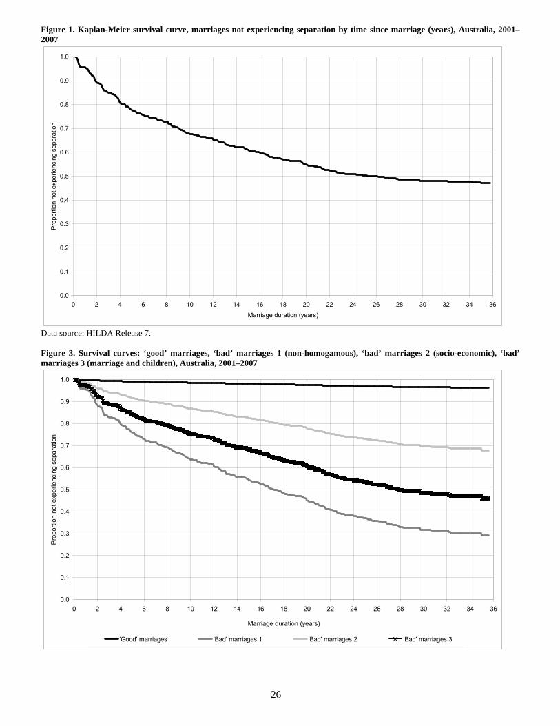
who drinks more than her husband is associated with a two-thirds greater hazard of separation (Table 3, Model 1). However homogamy in terms of country of birth and religiosity are not important (Table 3). The independence hypothesis postulates that women are more likely to leave a marriage if they have the resources to do so, measured in terms of education and connection to the labour force. Using Australian data we find no support for this. Wife’s education, employment status and years in paid work have no significant correlation with the risk of marital separation (Table 3). However we find that some economic variables—particularly those signalling financial stress—are important. Controlling for other variables, couples with an equivalised househould income of less than $20,000 (roughly the bottom 25 per cent of the sample) have twice the separation risk of couples with an equivalised househould income of between $30,000 and $40,000 (corresponding to the second highest quintile). An unemployed husband has more than three times the risk of separation of a working man. In Model 2, unions in which the husband indicates that his family is very poor, poor, or just getting by are associated with an increased risk of two-thirds over couples in which both partners signal they are comfortable, very comfortable or prosperous (Table 3). Other variables associated with marital instability are as follows. Separation of the parents of one or both spouses increases the probability that they will also separate, as does a second-plus marriage for both partners. Interestingly, the former result is more significant than the latter. That is, in terms of union dissolution risk, it is more important that a person’s parents’ marriage dissolved than that the person had a previous marriage of their own which ended. A husband’s age at marriage under 25 years doubles the risk of separation. Resident children born before marriage, either to the couple or in a previous union, lift the separation hazard by almost two-thirds. The number and age of resident children have no effect, however the wife’s desire for a(nother) child significantly reduces the risk of separation. In Model 1, marriages in which only one partner is dissatisfied with the relationship have reduced risk of separation compared to marriages in which both spouses are dissatisfied. Satisfaction of both partners is associated with a separation hazard one-fifth that of unions in which both spouses are dissatisfied. ‘Good’ and ‘bad’ marriages Using the analysis outlined above, we can identify characteristics from the data associated with ‘good’ marriages—those at lower risk of dissolution—and those correlated with ‘bad’ marriages. In terms of ‘good’ marriages, our laundry list might read (from Model 2): a. Husband 1 year younger to 3 years older than his wife b. Husband and wife have similar preference for a(nother) child c. Husband and wife have same level of education d. Both 0-2 standard drinks per day e. Both do not smoke f. Equivalised household income is $30,000–$39,999

15

g. Husband works 35 or more hours per week h. Husband perceives the family as comfortable to prosperous i. Both sets of parents did not separate/divorce j. Husband’s age at marriage is 30–34 years k. First marriage for both l. No children born before marriage m. Wife ‘8’ on would like another child The survival curve for marriages with these characteristics is shown in Figure 3 (‘good’ marriages). The probability of separation is less than one per cent over the first five years, and less than four per cent over 35 years. In contrast, ‘bad’ marriages in terms of (1) homogamy, (2) socio-economic variables, and (3) marriage and children variables can be defined respectively. In terms of (1) homogamy, characteristics associated with increased separation hazard include: a. Husband 9 or more years older than his wife b. Wife 5–10 points higher than husband on preference for a(nother) child c. Husband’s education much higher than wife’s education d. Husband 0–2 drinks, wife 3+ drinks e. Husband does not smoke, wife smokes For (2) socio-economic variables: f. Equivalised household income is under $20,000 g. Husband is unemployed h. Husband perceives the family as very poor to just getting by For (3) marriage and children: i. Both sets of parents separated/divorced j. Husband’s age at marriage is under 25 years k. Second-plus marriage for both l. Children born before marriage m. Wife ‘2’ on would like another child Survival curves for these three sets of characteristics are also shown in Figure 3. It is assumed that characteristics not listed are as for ‘good’ marriages. The combination of characteristics for the first set of ‘bad’ marriages—where partners are set to be non-homogamous in age, preferences for children, education, and drinking and smoking behaviours—results in a cumulative separation risk of one-quarter over the first five years of marriage and 70 per cent over 35 years. Eight per cent of ‘bad’ marriages 2—with low incomes and unemployed and financially stressed husbands—dissolve after five years, and 32 per cent after 35 years. ‘Bad’ marriages 3—associated with risky marriage-and-children characteristics—would experience separation rates of 16 per cent after five years and 52 per cent after 35 years.

16

Conclusion Our research on the determinants of marital (in)stability utilises the unusual strengths of HILDA in two main ways. First, in terms of method we have, for one of the first times, exploited a strength of panel data by incorporating the effects on marital separation of changes over time in the independent variables. Second, because HILDA has similar information on all adult family members, the analysis has been able to determine relationships dyadically; that is, by testing interactive effects between variables measured for each of the individuals in a couple. As well, we have been able to use the technique of varying covariates which, in combination with the usefulness of the data, suggest strongly that we should have significant confidence in the veracity of the findings when considered in the context of the literature. We have been able to test: the role of homogamy (similarities between partners); the efficacy of the so-called ‘independence hypothesis’ (are women with greater market opportunities more likely to separate); and the impact of socio-economic and marriage-and-children variables. With respect to the first, couple concordance in age, preferences for future children, education and smoking and drinking practices are associated with marital stability. Perhaps surprisingly, we find that differences in country of birth and religiosity are not associated with separation. Non-homogamy variables, those that are not a reflection of similarities or differences between spouses, can be critical to marital stability or instability. The most important of these from our exercise are level of relationship satisfaction, household income, unemployment of the husband, and husband’s age at marriage. In line with work by de Vaus et al. (2003; 2005) we find only a weak link between cohabitation and subsequent marital separation. We also confirm strongly the negative association between marriage duration and the probability of separation, although issues of endogeneity necessarily mean that a straightforward interpretation of this association is not forthcoming. It is clear that characteristics of men and women can have quite different impacts on marital stability. Unemployment of the husband, but not the wife, and perceived financial stress by the husband, but not the wife, are associated with increased risk of marital separation. Similarly, a wife with a much stronger desire than her husband for a future child raises the risk of separation. However the reverse situation only does so in Model 2, and not to the same extent. Our analysis also provides insights into the independence hypothesis—the notion that marriages are more likely to last the more clearly defined are marital gender roles, and the less it appears that woman are able to be economically independent. We find no evidence for this proposition, in terms of the role of female education and labour market status. This might, of course, be a relatively recent phenomenon. Acknowledgements Analysis in this paper was carried out using Stata. This paper uses confidentialised unit record file from the Household, Income and Labour Dynamics in Australia (HILDA) survey. The HILDA Project was initiated and is funded by the Commonwealth Department of Families, Housing, Community Services and Indigenous Affairs (FaHCSIA) and is managed by the Melbourne Institute of Applied Economic and Social Research (MIAESR). The findings and

17

views reported in this paper, however, are those of the authors and should not be attributed to either FaHCSIA or the MIAESR. An earlier version of this paper was presented at the Biennial HILDA Survey Research Conference, 16–17 July 2009, Melbourne. Thanks go to Ruth Weston for valuable comments on an early draft of this paper. References

Amato, P.R. (1996). Explaining the intergenerational transmission of divorce. Journal of Marriage and the Family, 58(3): 628–640.

Amato, P. (2000). The consequences of divorce for adults and children. Journal of Marriage and the Family, 62(4): 1269–1287.

Amato, P. (2001). Children of divorce in the 1990s: an update of the Amato and Keith (1991) meta-analysis. Journal of Family Psychology, 15(3): 355–370.

Australian Bureau of Statistics [ABS] (2006). Household Expenditure Survey and Survey of Income and Housing: User Guide, catalogue number 6503.0, Canberra.

Australian Bureau of Statistics [ABS] (2009). Consumer Price Index Australia, catalogue number 6401.0, Canberra.

Becker, G.S. (1973). A theory of marriage: part 1. Journal of Political Economy, 81(4): 813–846.

Becker, G.S., Landes, E.M. and Michael, R.T. (1977). An economic analysis of marital instability. Journal of Political Economy, 85(6): 1141–1187.

Bracher, M., Santow, G., Morgan, S.P. and Trussell, J. (1993). Marriage dissolution in Australia: models and explanations. Population Studies, 47(3): 403–425.

Bradbury, B. and Norris, K. (2005). Income and separation. Journal of Sociology, 41(4): 425–446.

Bratter, J.L. and King, R.B. (2008). “But will it last?”: Marital instability among interracial and same-race couples. Family Relations, 57(2): 160–171.

Bumpass, L.L. and Sweet, J.A. (1972). Differentials in marital instability: 1970. American Sociological Review, 37(6): 754–766.

Bumpass, L.L., Martin, T.C. and Sweet, J.A. (1991). The impact of family background and early marital factors on marital disruption. Journal of Family Issues, 12(1): 22–42.

Butterworth, P., Oz, T., Rodgers, B. and Berry, H. (2008). Factors associated with relationship dissolution of Australian families with children. Social Policy Research Paper No. 37, Australian Government Department of Families, Housing, Community Services and Indigenous Affairs, Canberra.

Butterworth, P. and Rodgers, B. (2008). Mental health problems and marital disruption: is it the combination of husbands and wives’ mental health problems that predicts later divorce?. Social Psychiatry and Psychiatric Epidemiology, 43(9):758–763.

Caces, M.F., Harford, T.C., Williams, G.D. and Hanna, E.Z. (1999). Alcohol consumption and divorce rates in the United States. Journal of Studies on Alcohol, 60(5): 647–652.

Chan, T.W. and Halpin, B. (2003). Union dissolution in the United Kingdom. International Journal of Sociology, 32(4): 76–93.

18

Clarkwest, A. (2007). Spousal dissimilarity, race, and marital dissolution. Journal of Marriage and Family, 69(3): 639–653.

Cleves, M.A., Gould, W.W. and Gutierrez, R.G. (2004). An Introduction to Survival Analysis Using Stata, Stata Corporation, Texas.

Compton, J. (2009). Why do smokers divorce? Time preference and marital stability. Department of Economics, University of Manitoba, Winnipeg.

Coombs, L.C. and Zumeta, Z.(1970). Correlates of marital dissolution in a prospective fertility study: a research note. Social Problems, 18(1): 92–102.

Cox, D.R. (1972). Regression models and life tables. Journal of the Royal Statistical Society. Series B (Methodological), 34(2): 187–220.

de Vaus, D., Qu, L. and Weston, R. (2003). Premarital cohabitation and subsequent marital stability. Family Matters, 65: 34–39.

de Vaus, D., Qu, L. and Weston, R. (2005). The disappearing link between premarital cohabitation and subsequent marital stability, 1970–2001. Journal of Population Research, 22(2): 99–118.

de Vaus, D., Gray, M., Qu, L. and Stanton, D. (2007). The consequences of divorce for financial living standards in later life. Research Paper 38, Australian Institute of Family Studies, Melbourne.

De Maris, A. (2004). Regression with Social Data: Modeling Continuous and Limited Response Variables, John Wiley & Sons, New Jersey.

Fu, H. and Goldman, N. (2000). The association between health-related behaviours and the risk of divorce in the USA. Journal of Biosocial Science, 32(1): 63–88.

Gray, M. and Chapman, B. (2007). Relationship breakdown and the economic welfare of Australian mothers and their children. Australian Journal of Labour Economics, 10(4): 251–275.

Hansen, H. (2005). Unemployment and marital dissolution: a panel data study of Norway. European Sociological Review, 21(2): 135–148.

Hewitt, B. (2008). Marriage breakdown in Australia: social correlates, gender and initiator status. Social Policy Research Paper No. 35, Australian Government Department of Families, Housing, Community Services and Indigenous Affairs, Canberra.

Hewitt, B., Baxter, J. and Western, M. (2005). Marriage breakdown in Australia: the social correlates of separation and divorce. Journal of Sociology, 41(2): 163–183.

Hewitt, B., Western, M. and Baxter, J. (2006). Who decides? The social characteristics of who initiates marital separation. Journal of Marriage and Family, 68(5): 1165–1177.

Hewitt, B. and de Vaus, D. (2009). Change in the association between premarital cohabitation and separation, Australia, 1945–2000. Journal of Marriage and Family, 71(2): 353–361.

Hohmann-Marriott, B.E. (2006). Shared beliefs and the union stability of married and cohabiting couples. Journal of Marriage and Family, 68(4): 1015–1028.

Homish, G.G. and Leonard, K.E. (2007). The drinking partnership and marital satisfaction: the longitudinal influence of discrepant drinking. Journal of Consulting and Clinical Psychology, 75(1): 43–51.

19

House of Representatives Standing Committee on Legal and Constitutional Affairs [HOR] (1998). To Have and to Hold: Strategies to Strengthen Marriage and Relationships, Parliamentary Paper 95/1998, Commonwealth of Australia, Canberra.

Jain, S. (2007). Lifetime marriage and divorce trends. Australian Social Trends, Australian Bureau of Statistics, catalogue number 4102.0, Canberra.

Jalovaara, M. (2003). The joint effects of marriage partners’ socioeconomic positions on the risk of divorce. Demography, 40(1): 67–81.

Jensen, P. and Smith, N. (1990). Unemployment and marital dissolution. Journal of Population Economics, 3(3): 215–229.

Kalmijn, M. and Poortman, A. (2006). His or her divorce? The gendered nature of divorce and its determinants. European Sociological Review, 22(2): 201–214.

Kiernan, K. and Mueller, G. (1999). Who divorces? in S. McRae (ed.) Changing Britain: Families and Households in the 1990s, Oxford University Press, Oxford, 377–403.

Lehrer, E.L. (2004). Religion as a determinant of economic and demographic behavior in the United States. Population and Development Review, 30(4): 707–726.

Lehrer, E.L. (2008). Age at marriage and marital instability: revisiting the Becker–Landes–Michael hypothesis. Journal of Population Economics, 21(2): 463–484.

Lyngstad, T.H. (2004). The impact of parents’ and spouses’ education on divorce rates in Norway. Demographic Research, 10(5): 121–142.

Ortega, S.T., Whitt, H.P. and Williams Jr, J.A. (1988). Religious homogamy and marital happiness. Journal of Family Issues, 9(2): 224–239.

Ostermann, J., Sloan, F.A. and Taylor, D.H. (2005). Heavy alcohol use and marital dissolution in the USA. Social Science and Medicine, 61(11): 2304–2316.

Poortman, A. and Lyngstad, T.H. (2007). Dissolution risks in first and higher order marital and cohabiting unions. Social Science Research, 36(4): 1431–1446.

Power, C. and Estaugh, V. (1990). The role of family formation and dissolution in shaping drinking behaviour in early adulthood. British Journal of Addiction, 85(4): 521–530.

Ross, H.L. and Sawhill, I.V. (1975). Time of Transition: The Growth of Families Headed By Women, The Urban Institute, Washington D.C.

Smith, I. (1997). Explaining the growth of divorce in Great Britain. Scottish Journal of Political Economy, 44(5): 519–544.

Teachman, J.D. (2002). Stability across cohorts in divorce risk factors. Demography, 39(2): 331–351.

Thomson, E. (1997). Couple childbearing desires, intentions, and births. Demography, 34(3): 343–354.

Tzeng, J.M. (1992). The effects of socioeconomic heterogamy and changes on marital dissolution for first marriages. Journal of Marriage and the Family, 54(3): 609–619.

Wagner, M. and Weiss, B. (2006). On the variation of divorce risks in Europe: findings from a meta-analysis of European longitudinal studies. European Sociological Review, 22(5): 483–500.

Weiss, Y. and Willis, R.J. (1997). Match quality, new information and marital dissolution. Journal of Labor Economics, 15(1): S293–S329.

20

Wolcott, I. and Hughes, J. (1999). Towards understanding the reasons for divorce. Working Paper 20, Australian Institute of Family Studies, Melbourne.

Wolfinger, N.H. (2003). Family structure homogamy: the effects of parental divorce on partner selection and marital stability. Social Science Research, 32(1): 80–97.

Zeiss, A.M., Zeiss, R. and Johnson, S. (1981). Sex differences in initiation of and adjustment to divorce. Journal of Divorce and Remarriage, 4(2): 21–33.

21

Table 1. Data description. Sample by sex and other covariates in wave 1, and % separated by wave 7 Males Females Covariate Number % separated Number % separated Total 2,482 10.7 2,482 10.7 Current age 18–29 years 197 19.8 301 17.6 30–39 years 781 13.4 940 12.6 40–49 years 901 10.2 837 9.0 50–58 years 603 5.0 404 5.0 Education Bachelor degree or above 599 8.8 564 8.9 Other post-school qualification 1,037 11.6 546 11.5 Completed high school 239 12.1 404 11.9 Did not complete high school 607 10.5 967 10.9 Equivalised household income Under $20,000 636 14.6 $20,000–$29,999 759 10.7 $30,000–$39,999 557 8.8 $40,000+ 530 8.1 Employment status Works 0–34 hours per week 158 10.8 907 10.4 Works 35+ hours per week 2,064 10.5 792 10.0 Unemployed 69 20.3 58 20.7 Not in the labour force 190 9.5 725 11.2 Years in paid employment 0–14 years 447 17.4 1,159 12.4 15–19 years 390 11.8 483 11.8 20–29 years 908 11.1 637 8.3 30+ years 734 5.6 202 5.9 Length of marriage 0–4 years 474 17.7 5–9 years 428 14.5 10–19 years 801 10.9 20+ years 779 4.2 Age at marriage Under 25 years 1,013 10.1 1,416 9.5 25–29 years 764 9.0 604 9.9 30–34 years 400 11.3 283 13.4 35+ years 304 16.4 179 19.0 Lived together before this marriage No 1,332 6.4 Yes 1,150 15.7 Children before this marriage No 2,067 8.9 Yes 415 19.8 Number of resident children 0 596 8.4 1 510 12.7 2 839 11.1 3+ 537 10.8 Age of youngest resident child 0–4 years 685 14.2 5–14 years 791 11.6 15+ years 408 6.6 Like to have a(nother) child Would not like (0–2) 1,586 10.3 1,721 9.8 Unsure (3–7) 271 12.9 226 15.0 Would like (8–10) 428 13.1 456 13.2 Data source: HILDA Release 7.

22

Table 2. Dyadic data description. Sample characteristics in wave 1, and % separated by wave 7 Covariate Number % separated Country of birth Both born in Australia 1,572 10.8 Both born in same country (not Australia) 296 8.1 Born in different countries 614 11.7 Age difference Husband 1 year younger to 3 years older 1,463 9.5 Husband 4–8 years older 597 9.4 Husband 9+ years older 155 16.8 Husband 2+ years younger 267 16.9 Difference in preference for a(nother) child Husband and wife have similar preference [–1 ≤ W–H ≤ 1] 1,778 9.8 Wife moderately stronger preference [2 ≤ W–H ≤ 4] 135 15.6 Wife much stronger preference [5 ≤ W–H ≤ 10] 112 17.9 Husband moderately stronger preference [–4 ≤ W–H ≤ –2] 124 16.1 Husband much stronger preference [–10 ≤ W–H ≤ –5] 119 14.3 Religiosity Both religion is unimportant (0–4) 785 13.6 Husband unimportant, Wife important 541 10.4 Husband important, Wife unimportant 217 12.0 Both important (5–10) 936 8.1 Difference in education Both same level of education 960 9.5 Husband much higher 639 11.3 Husband higher 351 12.3 Husband lower 316 11.7 Husband much lower 215 10.7 Standard drinks per day Both 0–2 1,102 8.9 Husband 0–2, Wife 3+ 136 14.0 Husband 3+, Wife 0–2 673 10.1 Both 3+ 341 15.0 Smoking Both do not smoke 1,598 8.0 Husband does not smoke, Wife smokes 305 14.1 Husband smokes, Wife does not smoke 177 14.7 Both smoke 235 20.4 Satisfaction with life Both dissatisfied (0–7) 292 14.7 Husband dissatisfied, Wife satisfied 473 13.3 Husband satisfied, Wife dissatisfied 360 14.2 Both satisfied (8–10) 1,353 8.1 Satisfaction with relationship Both dissatisfied (0–7) 211 21.8 Husband dissatisfied, Wife satisfied 166 20.5 Husband satisfied, Wife dissatisfied 237 15.2 Both satisfied (8–10) 1,681 7.5 Perceived prosperity Both comfortable to prosperous 1,376 7.9 Husband comfortable to prosperous, Wife very poor to just getting by 210 12.4 Husband very poor to just getting by, Wife comfortable to prosperous 239 13.4 Both very poor to just getting by 483 16.6 Parents ever separated/divorced Both sets did not separate/divorce 1,730 8.2 Husband’s separated, wife’s did not 318 14.5 Husband’s did not separate, wife’s did 358 17.0 Both sets separated/divorced 76 22.4 Marriage order Both 1st marriage 1,996 9.7 Husband’s 1st marriage, Wife’s 2nd+ marriage 177 11.3 Husband’s 2nd+ marriage, Wife’s 1st marriage 160 13.8 Both 2nd+ marriage 149 20.1 Data source: HILDA Release 7.

23

Table 3. Cox regression results, dyadic analysis, marital dissolution across 7 waves by selected covariates MODEL 1 MODEL 2

Covariate Hazard ratio p-value Hazard ratio p-value Homogamous Country of birth Ref cat: Both born in Australia Both born in same country (not Australia) 1.033 0.911 1.112 0.699 Both born in different countries 0.825 0.267 0.887 0.486 Age Ref cat: Husband –1 to 3 years older Husband 4–8 years older 1.402 0.083 1.315 0.152 Husband 9+ years older 2.235 0.019 1.853 0.068 Husband 2+ years younger 1.526 0.044 1.443 0.078 Preference for a(nother) child Ref cat: Husband and wife have similar preference Wife moderately stronger preference 1.305 0.367 1.543 0.138 Wife much stronger preference 1.980 0.038 2.639 0.003 Husband moderately stronger preference 1.160 0.587 1.313 0.315 Husband much stronger preference 1.343 0.257 1.593 0.068 Religiosity Ref cat: Both religion is unimportant (0–4) H unimportant, W important 0.991 0.964 0.990 0.958 H important, W unimportant 1.119 0.621 1.221 0.377 Both important (5–10) 0.882 0.529 0.848 0.397 Education Ref cat: Both same level of education Husband much higher 1.730 0.021 1.721 0.020 Husband higher 1.564 0.058 1.656 0.033 Husband lower 1.287 0.291 1.198 0.447 Husband much lower 0.919 0.765 0.874 0.630 Standard drinks per day Ref cat: Both 0–2 Husband 0–2, Wife 3+ 1.650 0.067 1.689 0.054 Husband 3+, Wife 0–2 1.113 0.548 1.073 0.696 Both 3+ 1.265 0.245 1.386 0.102 Smoking Ref cat: Both do not smoke Husband does not smoke, Wife smokes 1.954 0.000 2.314 0.000 Husband smokes, Wife does not smoke 1.756 0.019 2.076 0.002 Both smoke 1.469 0.089 1.476 0.082 Satisfaction Satisfaction with life Ref cat: Both dissatisfied (0–7) Husband dissatisfied, Wife satisfied 0.822 0.373 Husband satisfied, Wife dissatisfied 1.075 0.736 Both satisfied (8–10) 0.853 0.433 Satisfaction with relationship Ref cat: Both dissatisfied (0–7) Husband dissatisfied, Wife satisfied 0.639 0.037 Husband satisfied, Wife dissatisfied 0.491 0.001 Both satisfied (8–10) 0.184 0.000 Data source: HILDA Release 7.

24

Table 3 cont. Cox regression results, dyadic analysis, marital dissolution across 7 waves by selected covariates MODEL 1 MODEL 2 Covariate Hazard ratio p-value Hazard ratio p-value Socio-economic Wife’s education Ref cat: Bachelor degree or above Other post-school qualifications 1.018 0.939 0.897 0.640 Completed high school 0.930 0.796 0.757 0.320 Did not complete high school 0.820 0.512 0.682 0.201 Equivalised household income Ref cat: Under $20,000 $20,000–$29,999 0.855 0.410 0.911 0.623 $30,000–$39,999 0.506 0.005 0.550 0.014 $40,000+ 0.774 0.320 0.827 0.467 Husband’s employment status Ref cat: Works 0–34 hours per week Works 35+ hours per week 1.039 0.887 1.095 0.737 Unemployed 3.318 0.019 3.652 0.010 Not in the labour force 0.7045 0.474 0.613 0.309 Wife’s employment status Ref cat: Works 0–34 hours per week Works 35+ hours per week 1.236 0.203 1.252 0.171 Unemployed 1.424 0.407 1.613 0.256 Not in the labour force 0.749 0.225 0.683 0.106 Husband’s years in paid employment 0.966 0.067 0.969 0.084 Wife’s years in paid employment 0.999 0.916 0.993 0.615 Perceived prosperity Ref cat: Both comfortable to prosperous H comfortable/prosperous, W very poor/just getting by 0.646 0.151 0.748 0.340 H very poor/just getting by, W comfortable/prosperous 1.318 0.204 1.664 0.018 Both very poor to just getting by 1.317 0.135 1.706 0.003 Marriage and children Parents ever separated/divorced Ref cat: Both sets did not separate/divorce Husband’s separated, wife’s did not 1.845 0.002 1.739 0.004 Husband’s did not separate, wife’s did 1.610 0.011 1.550 0.016 Both sets separated/divorced 1.774 0.059 2.008 0.019 Husband’s age at marriage Ref cat: under 25 years 25–29 years 0.507 0.001 0.498 0.000 30–34 years 0.403 0.001 0.428 0.002 35+ years 0.477 0.078 0.579 0.184 Marriage order Ref cat: Both 1st marriage H 2nd+ marriage, W 1st marriage 0.762 0.412 0.761 0.407 H 1st marriage, W 2nd+ marriage 0.730 0.316 0.912 0.761 Both 2nd+ marriage 1.781 0.072 1.768 0.071 Lived together before this marriage Ref cat: No Yes 1.292 0.151 1.377 0.071 Children before this marriage Ref cat: No Yes 1.632 0.019 1.498 0.051 Number of resident children Ref cat: 0 1 2.251 0.192 2.450 0.147 2 2.751 0.105 2.531 0.135 3+ 1.589 0.472 1.534 0.504 Age of youngest resident child 1.000 0.960 0.993 0.728 Wife would like to have a(nother) child 0.937 0.051 0.918 0.008

25

Data source: HILDA Release 7.

26

Figure 1. Kaplan-Meier survival curve, marriages not experiencing separation by time since marriage (years), Australia, 2001–2007

0.0

0.1

0.2

0.3

0.4

0.5

0.6

0.7

0.8

0.9

1.0

0 2 4 6 8 10 12 14 16 18 20 22 24 26 28 30 32 34 36

Marriage duration (years)

Pro

port

ion

not

exp

erie

ncin

g se

para

tion

Data source: HILDA Release 7. Figure 3. Survival curves: ‘good’ marriages, ‘bad’ marriages 1 (non-homogamous), ‘bad’ marriages 2 (socio-economic), ‘bad’ marriages 3 (marriage and children), Australia, 2001–2007

0.0

0.1

0.2

0.3

0.4

0.5

0.6

0.7

0.8

0.9

1.0

0 2 4 6 8 10 12 14 16 18 20 22 24 26 28 30 32 34 36

Marriage duration (years)

Pro

port

ion

not

expe

rienc

ing

sepa

ratio

n

'Good' marriages 'Bad' marriages 1 'Bad' marriages 2 'Bad' marriages 3

27

Figure 2. Monthly hazard of separation associated with Figure 1’s Kaplan-Meier survival curve, Australia, 2001–2007

0.0000

0.0002

0.0004

0.0006

0.0008

0.0010

0.0012

0.0014

0 2 4 6 8 10 12 14 16 18 20 22 24 26 28 30 32 34 36

Marriage duration (years)

Mon

thly

haz

ard

of s

epar

atio

n