Nuclear Instruments and Methods in Physics Research A 654 (2011) 653–660

Contents lists available at ScienceDirect

Nuclear Instruments and Methods inPhysics Research A

0168-90

doi:10.1

� Corr

E-m

journal homepage: www.elsevier.com/locate/nima

The atmospheric transparency measured with a LIDAR system at theTelescope Array experiment

Takayuki Tomida a,�, Yusuke Tsuyuguchi a, Takahito Arai b, Takuya Benno c, Michiyuki Chikawa c,Koji Doura c, Masaki Fukushima d, Kazunori Hiyama d, Ken Honda a, Daisuke Ikeda d, John N. Matthews e,Toru Nakamura f, Daisuke Oku a, Hiroyuki Sagawa d, Hisao Tokuno g, Yuichiro Tameda d,Gordon B. Thomson e, Yoshiki Tsunesada g, Shigeharu Udo h, Hisashi Ukai a

a Interdisciplinary Graduate School of Medicine and Engineering, Mechanical Systems Engineering, University of Ymanashi, Kofu, Yamanashi 400-8511, Japanb Research Institute for Science and Technology, Kinki University, Higashiosaka, Osaka 577-8502, Japanc Department of Physics, Kinki University, Higashiosaka, Osaka 577-8502, Japand Institute for Cosmic Ray Research, University of Tokyo, Kashiwa, Chiba 277-8582, Japane Institute for High Energy Astrophysics and Department of Physics, University of Utah, Salt Lake City, UT 84112-0830, USAf Kochi University, Faculty of Science, Kochi 780-8520, Japang Graduate School of Science and Engineering, Tokyo Institute of Technology, Meguro, Tokyo 152-8551, Japanh Kanagawa University, Yokohama, Kanagawa 221-8686, Japan

a r t i c l e i n f o

Article history:

Received 21 September 2010

Received in revised form

9 April 2011

Accepted 8 July 2011Available online 26 July 2011

Keywords:

Ultra High Energy Cosmic Rays

Fluorescence

Atmospheric transparency

LIDAR

02/$ - see front matter & 2011 Elsevier B.V. A

016/j.nima.2011.07.012

esponding author. Tel.: þ81 55 220 8418.

ail address: g08dm003@yamanashi.ac.jp (T. T

a b s t r a c t

An atmospheric transparency was measured using a LIDAR with a pulsed UV laser (355 nm) at the

observation site of Telescope Array in Utah, USA. The measurement at night for two years in 2007–2009

revealed that the extinction coefficient by aerosol at the ground level is 0:033þ0:016�0:012 km�1 and the

vertical aerosol optical depth at 5 km above the ground is 0:035þ0:019�0:013 . A model of the altitudinal aerosol

distribution was built based on these measurements for the analysis of atmospheric attenuation of the

fluorescence light generated by ultra high energy cosmic rays.

& 2011 Elsevier B.V. All rights reserved.

1. Introduction

Ultra High Energy Cosmic Rays (UHECRs) interact with thecosmic microwave background and produce a cutoff structure intheir energy spectrum (GZK cutoff) at the energy around 1019:8 eVas predicted by Greisen et al. [1,2]. The HiRes group reported thatthere is a GZK cut-off in their observed energy spectrum at theenergy it was predicted [3,4]. A similar suppression in the energyspectrum is reported by the Auger experiment in the SouthernHemisphere [5]. However, the AGASA experiment observed aspectrum which continued unabatedly with 11 events beyondthe GZK cutoff [6,7]. To understand this discrepancy, the Tele-scope Array (TA) experiment was constructed in the desert areanear the town of Delta in Utah, the USA. It is a hybrid detectorconsisting of Surface Detector (SD) array and three Fluores-cence Detector (FD) stations. It measures the energy spectrum,

ll rights reserved.

omida).

anisotropy and composition of UHECRs to identify their origin.The TA has three FD stations called ‘‘Black Rock Mesa’’ (BR), ‘‘LongRidge’’ (LR) and ‘‘Middle Drum’’ (MD), which have been installedsurrounding the SD array. The BR site (1404 m a.s.l.) is located atthe southeast corner of the SD array while the LR site (1554 ma.s.l.) is to the southwest. The BR and LR stations each have 12telescopes. The MD site (1610 m a.s.l.) is located at the northwest,and has 14 telescopes. The FD stations overlook an array of 507SDs (Fig. 1).

The UV fluorescence light generated by an air shower isscattered and lost along the path of transmission to the telescope.The main scattering processes are Rayleigh scattering by mole-cules and scattering by aerosols in the atmosphere. The Rayleighscattering process is well understood and the attenuation lengthcan be calculated using the Rayleigh scattering cross-section andthe molecular densities of the atmosphere [8–10]. In order tocalculate the molecular densities of the atmosphere, radiosondedata from Elko(Nevada) are used to obtain temperature, pressureand humidity around the TA observatory as a function of height.Sizes, shapes and spatial distribution of aerosols around the site

Fig. 1. Location of the LIDAR system. A left figure is a map of the TA experiment. Little black points are SDs, and three FD stations are shown by BR, LR, and MD. A right

picture shows the positions of BR-station and LIDAR dome. (For interpretation of the references to color in this figure legend, the reader is referred to the web version of

this article.)

T. Tomida et al. / Nuclear Instruments and Methods in Physics Research A 654 (2011) 653–660654

are not known, and are variable with time. Therefore, on-sitemonitoring of aerosols is essential in a fluorescence experiment.

In the TA, we employ a variety of measurements for atmo-spheric monitoring, using two laser systems and a cloud camera.The first laser system is the LIDAR (LIght Detection And Ranging,we call LIDAR) installed near the BR station, which injects apulsed laser light in the atmosphere and observes the back-scattered light at the same location. LIDAR is widely used inground based aerosol measurement. The LIDAR system is oper-ated before the beginning and after the end of an FD observation,twice a night. The second laser system is located at the geogra-phical center of the three FD stations. It fires a vertical laser beamof 355 nm and the scattered light by the atmosphere is observedby each fluorescence detector station. This system is called CLF(Central Laser Facility) [11,12]. We are shooting 300 shots of laserat 10 Hz from the CLF every 30 min during FD observation. Inaddition, we installed an infrared CCD camera for cloud monitor-ing near the LIDAR system, and take pictures of the night skyevery hour during FD observation [13]. Furthermore, the weathermonitors are installed in each of the FD stations and at the CLF toobtain the atmospheric status at the ground level.

In this paper, we report on the LIDAR system (Section 2), thedata set and the analysis method (Section 3), the determination ofthe Rayleigh scattering by the radiosonde data (Section 4), theresult of aerosol scattering by the LIDAR data (Section 5), and amodel of atmospheric transparency at the TA site (Section 6).

2. LIDAR system

A photograph of the LIDAR system is shown Fig. 2(a). TheLIDAR is composed of five basic system blocks. Those are (1) alaser, (2) a steerable telescope, (3) a photo-multiplier tube, (4) adigital oscilloscope, and (5) a control system as shown in Fig. 2(b).We use an air cooled Nd:YAG laser (Orion model by New WaveResearch) with a third harmonic oscillation module (355 nm). Thelaser fires a pulse with the width of 4–6 ns at 1 Hz. The maximumenergy of the laser pulse is 4 mJ. A MEADE LX200GPS-30 tele-scope with a diameter of 305 mm and a focal length of 3048 mmis used with a photo-multiplier tube (HAMAMATSU R3479)mounted at the focus of the telescope. A linear range of the

PMT was checked by simultaneously firing a series of UV-LEDpulses at the telescope overlaying with the laser shot, andconfirming that the overlaid signal has the same charge as theLED-only signal without the laser shot. The laser is attached to thetelescope mount, therefore the direction control of the laser-telescope-PMT system can be simply accomplished by commandsto the telescope mount. The back-scattered photons from thelaser are collected by the telescope, detected by the PMT, and thesignals are digitized with a digital oscilloscope (Tektronix 3034B)[11,14]. In addition, a portion of each laser shot is picked off formeasurement by an energy monitor.

By measuring the time structure of the back-scatteredphotons, we can determine the atmospheric conditions includingaerosol distributions along the path of the laser beam. Theoperation of the LIDAR is composed of horizontal shots in thenorth and vertical shots. The vertical operation was made in highð � 4 mJÞ and low ð � 1 mJÞ energies in order to measure theextinction coefficient a over a large range. The horizontal opera-tion uses only the high energy. In each vertical and horizontaloperation, 500 laser pulses are shot and recorded. A total of 1500shots composed one LIDAR operation. The pedestal level ismeasured in between each shot and is subtracted from the lasershot data in order to account for the background. In the followinganalysis, we use an average of the PMT signal profiles in order toreduce shot-to-shot fluctuations.

3. Data set and analysis method

A waveform W(t) is obtained by averaging the PMT signal for500 laser shots. A range corrected power return F(x) of the LIDARis defined by the waveform W(t) as a function of the distance x

from the LIDAR:

FðxÞ ¼WðtÞx2, x¼ tc

2ð1Þ

where c is the speed of light and t is the time from the laser shot.The solid angle correction is taken into account in the definition ofF(x). An example of W(t) and F(x) is shown in Figs. 3 and 4.

Laser Head

TelescopePMT

Steering System

Directioncontrol (θ, φ)

LocalComputer Control

back scatteredphotons

Digitaloscilloscope

Laser beam

PO 1:10

Energy probe

ADC

(Ethernet)

Fig. 2. The LIDAR system. A left picture is LIDAR’s optical system (telescope, laser, etc.). A right picture is a connection block diagram of device of LIDAR. (a) LIDAR telescope

and laser (b) Block diagram of the LIDAR system.

-16

-14

-12

-10

-8

-6

-4

-2

0

2

-20 0 20 40 60 80 100 120 140 160

volta

ge [m

V]

time [us]

Fig. 3. Example of W(t) for horizontal shots.

0.0001

0.001

0.01

0.1

0 5 10 15 20

Sca

tterin

g ph

oton

inte

nsity

[V k

m2 ]

Distance from LIDAR [km]

Fig. 4. Example of F(x) as a function of the distance x.

T. Tomida et al. / Nuclear Instruments and Methods in Physics Research A 654 (2011) 653–660 655

The extinction coefficient aðxÞ at a distance x is related withF(x) by the LIDAR equation:

1

FðxÞ

dFðxÞ

dx¼

1

bðxÞdbðxÞ

dx�2aðxÞ ð2Þ

where b is the back-scattering coefficient. The factor 2 of aindicates a round-trip photon propagation.

If the atmosphere is spatially uniform along x, such as the casefor the horizontal shots, dbðxÞ=dx¼ 0 and F(x) becomes exponen-tial. We can exactly solve the equation and obtain the extinctioncoefficient aðxÞ (the slope method [15,16]).

In the case of vertical laser shots, where the atmosphericcondition (a and b) changes with x, we need an additionalassumption on the relation between a and b and also a boundary

condition to solve the equation. In Klett’s method [17,18], aboundary condition is assumed that a at enough high altitude isgiven by that of Rayleigh scattering because the aerosol scatteringcan be neglected at high altitude. The back-scattering coefficient bis assumed to be bpak. The value of k is 1.00 for the molecularatmosphere but is known to vary significantly ð0:67oko1:30Þfor the atmosphere heavily loaded by the aerosol or with rain andsnow [18–21]. However, for a typical desert atmosphere of the TAsite, we found that the aerosol contribution increases towards thelower altitude and that it modifies the value of k from 1.00 at thehigh altitude up to 1.14 near the ground. In solving Eq. (2) byKlett’s method, we assume that b is in proportion to a for thewhole interval of x. We estimate a systematic error caused by thisassumption by the iterative method (see Section 5).

0

2

4

6

8

10

12

14

0.054 0.056 0.058 0.06 0.062 0.064 0.066 0.068

Ent

ries

The extinction coefficient of Rayleigh [/km]

Extinction coefficient of Rayleigh

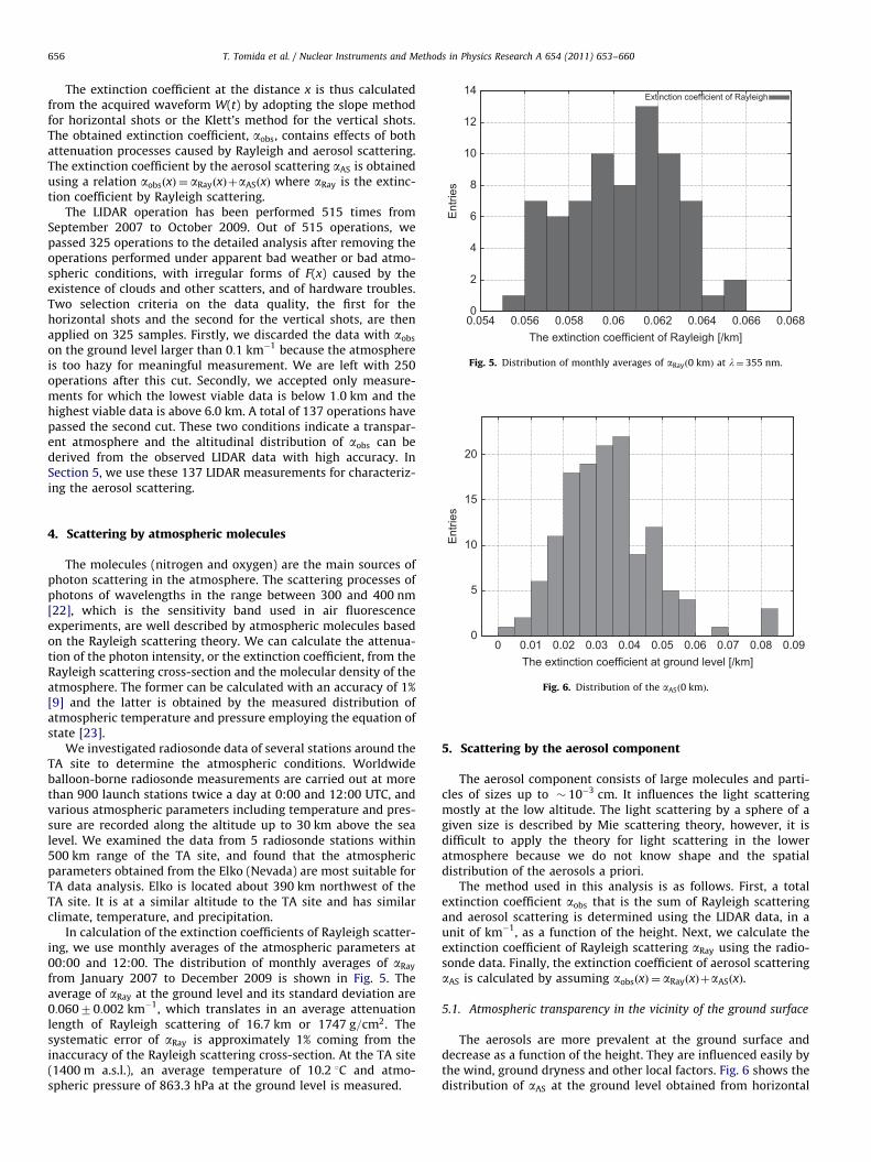
Fig. 5. Distribution of monthly averages of aRayð0 kmÞ at l¼ 355 nm.

20

T. Tomida et al. / Nuclear Instruments and Methods in Physics Research A 654 (2011) 653–660656

The extinction coefficient at the distance x is thus calculatedfrom the acquired waveform W(t) by adopting the slope methodfor horizontal shots or the Klett’s method for the vertical shots.The obtained extinction coefficient, aobs, contains effects of bothattenuation processes caused by Rayleigh and aerosol scattering.The extinction coefficient by the aerosol scattering aAS is obtainedusing a relation aobsðxÞ ¼ aRayðxÞþaASðxÞ where aRay is the extinc-tion coefficient by Rayleigh scattering.

The LIDAR operation has been performed 515 times fromSeptember 2007 to October 2009. Out of 515 operations, wepassed 325 operations to the detailed analysis after removing theoperations performed under apparent bad weather or bad atmo-spheric conditions, with irregular forms of F(x) caused by theexistence of clouds and other scatters, and of hardware troubles.Two selection criteria on the data quality, the first for thehorizontal shots and the second for the vertical shots, are thenapplied on 325 samples. Firstly, we discarded the data with aobs

on the ground level larger than 0:1 km�1 because the atmosphereis too hazy for meaningful measurement. We are left with 250operations after this cut. Secondly, we accepted only measure-ments for which the lowest viable data is below 1:0 km and thehighest viable data is above 6.0 km. A total of 137 operations havepassed the second cut. These two conditions indicate a transpar-ent atmosphere and the altitudinal distribution of aobs can bederived from the observed LIDAR data with high accuracy. InSection 5, we use these 137 LIDAR measurements for characteriz-ing the aerosol scattering.

0

5

10

15

0 0.01 0.02 0.03 0.04 0.05 0.06 0.07 0.08 0.09

Ent

ries

The extinction coefficient at ground level [/km]

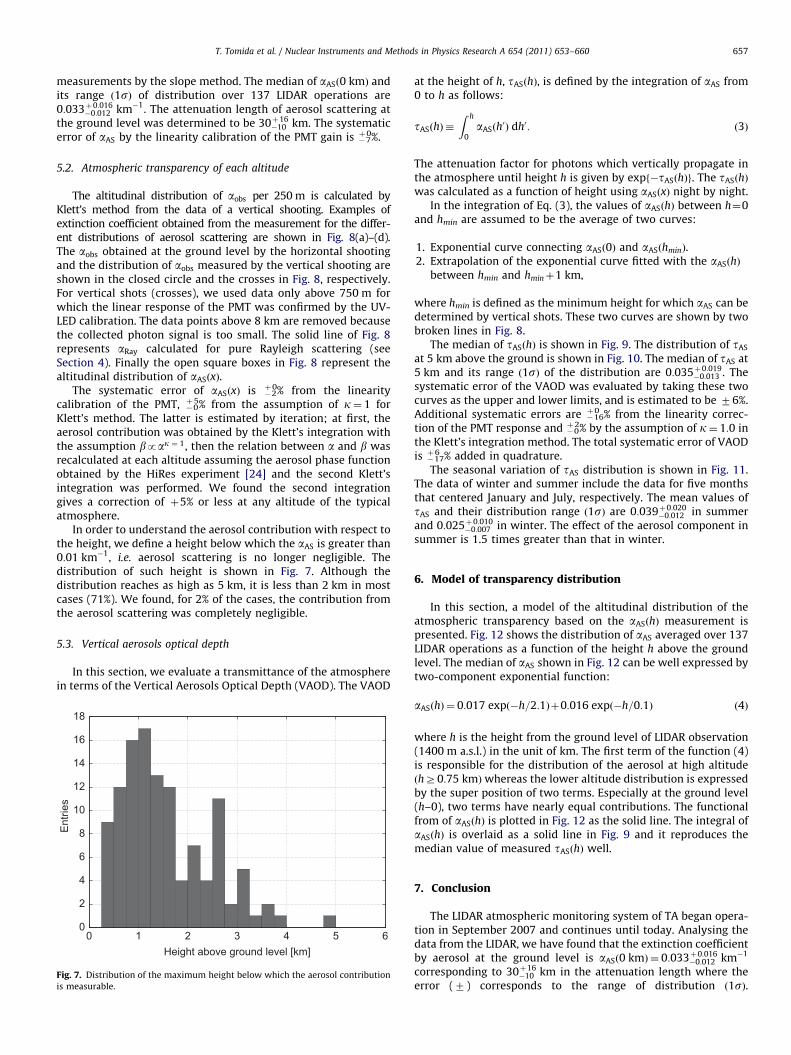
Fig. 6. Distribution of the aASð0 kmÞ.

4. Scattering by atmospheric molecules

The molecules (nitrogen and oxygen) are the main sources ofphoton scattering in the atmosphere. The scattering processes ofphotons of wavelengths in the range between 300 and 400 nm[22], which is the sensitivity band used in air fluorescenceexperiments, are well described by atmospheric molecules basedon the Rayleigh scattering theory. We can calculate the attenua-tion of the photon intensity, or the extinction coefficient, from theRayleigh scattering cross-section and the molecular density of theatmosphere. The former can be calculated with an accuracy of 1%[9] and the latter is obtained by the measured distribution ofatmospheric temperature and pressure employing the equation ofstate [23].

We investigated radiosonde data of several stations around theTA site to determine the atmospheric conditions. Worldwideballoon-borne radiosonde measurements are carried out at morethan 900 launch stations twice a day at 0:00 and 12:00 UTC, andvarious atmospheric parameters including temperature and pres-sure are recorded along the altitude up to 30 km above the sealevel. We examined the data from 5 radiosonde stations within500 km range of the TA site, and found that the atmosphericparameters obtained from the Elko (Nevada) are most suitable forTA data analysis. Elko is located about 390 km northwest of theTA site. It is at a similar altitude to the TA site and has similarclimate, temperature, and precipitation.

In calculation of the extinction coefficients of Rayleigh scatter-ing, we use monthly averages of the atmospheric parameters at00:00 and 12:00. The distribution of monthly averages of aRay

from January 2007 to December 2009 is shown in Fig. 5. Theaverage of aRay at the ground level and its standard deviation are0:06070:002 km�1, which translates in an average attenuationlength of Rayleigh scattering of 16.7 km or 1747 g=cm2. Thesystematic error of aRay is approximately 1% coming from theinaccuracy of the Rayleigh scattering cross-section. At the TA site(1400 m a.s.l.), an average temperature of 10.2 1C and atmo-spheric pressure of 863.3 hPa at the ground level is measured.

5. Scattering by the aerosol component

The aerosol component consists of large molecules and parti-cles of sizes up to � 10�3 cm. It influences the light scatteringmostly at the low altitude. The light scattering by a sphere of agiven size is described by Mie scattering theory, however, it isdifficult to apply the theory for light scattering in the loweratmosphere because we do not know shape and the spatialdistribution of the aerosols a priori.

The method used in this analysis is as follows. First, a totalextinction coefficient aobs that is the sum of Rayleigh scatteringand aerosol scattering is determined using the LIDAR data, in aunit of km�1, as a function of the height. Next, we calculate theextinction coefficient of Rayleigh scattering aRay using the radio-sonde data. Finally, the extinction coefficient of aerosol scatteringaAS is calculated by assuming aobsðxÞ ¼ aRayðxÞþaASðxÞ.

5.1. Atmospheric transparency in the vicinity of the ground surface

The aerosols are more prevalent at the ground surface anddecrease as a function of the height. They are influenced easily bythe wind, ground dryness and other local factors. Fig. 6 shows thedistribution of aAS at the ground level obtained from horizontal

T. Tomida et al. / Nuclear Instruments and Methods in Physics Research A 654 (2011) 653–660 657

measurements by the slope method. The median of aASð0 kmÞ andits range ð1sÞ of distribution over 137 LIDAR operations are0:033þ0:016

�0:012 km�1. The attenuation length of aerosol scattering atthe ground level was determined to be 30þ16

�10 km. The systematicerror of aAS by the linearity calibration of the PMT gain is þ0

�7%.

5.2. Atmospheric transparency of each altitude

The altitudinal distribution of aobs per 250 m is calculated byKlett’s method from the data of a vertical shooting. Examples ofextinction coefficient obtained from the measurement for the differ-ent distributions of aerosol scattering are shown in Fig. 8(a)–(d).The aobs obtained at the ground level by the horizontal shootingand the distribution of aobs measured by the vertical shooting areshown in the closed circle and the crosses in Fig. 8, respectively.For vertical shots (crosses), we used data only above 750 m forwhich the linear response of the PMT was confirmed by the UV-LED calibration. The data points above 8 km are removed becausethe collected photon signal is too small. The solid line of Fig. 8represents aRay calculated for pure Rayleigh scattering (seeSection 4). Finally the open square boxes in Fig. 8 represent thealtitudinal distribution of aASðxÞ.

The systematic error of aASðxÞ is þ0�2% from the linearity

calibration of the PMT, þ5�0% from the assumption of k¼ 1 for

Klett’s method. The latter is estimated by iteration; at first, theaerosol contribution was obtained by the Klett’s integration withthe assumption bpak ¼ 1, then the relation between a and b wasrecalculated at each altitude assuming the aerosol phase functionobtained by the HiRes experiment [24] and the second Klett’sintegration was performed. We found the second integrationgives a correction of þ5% or less at any altitude of the typicalatmosphere.

In order to understand the aerosol contribution with respect tothe height, we define a height below which the aAS is greater than0:01 km�1, i.e. aerosol scattering is no longer negligible. Thedistribution of such height is shown in Fig. 7. Although thedistribution reaches as high as 5 km, it is less than 2 km in mostcases (71%). We found, for 2% of the cases, the contribution fromthe aerosol scattering was completely negligible.

5.3. Vertical aerosols optical depth

In this section, we evaluate a transmittance of the atmospherein terms of the Vertical Aerosols Optical Depth (VAOD). The VAOD

0

2

4

6

8

10

12

14

16

18

0 1 2 3 4 5 6

Ent

ries

Height above ground level [km]

Fig. 7. Distribution of the maximum height below which the aerosol contribution

is measurable.

at the height of h, tASðhÞ, is defined by the integration of aAS from0 to h as follows:

tASðhÞ �

Z h

0aASðh

0Þ dh0: ð3Þ

The attenuation factor for photons which vertically propagate inthe atmosphere until height h is given by expf�tASðhÞg. The tASðhÞ

was calculated as a function of height using aASðxÞ night by night.In the integration of Eq. (3), the values of aASðhÞ between h¼0

and hmin are assumed to be the average of two curves:

1.

Exponential curve connecting aASð0Þ and aASðhminÞ. 2. Extrapolation of the exponential curve fitted with the aASðhÞ

between hmin and hminþ1 km,

where hmin is defined as the minimum height for which aAS can bedetermined by vertical shots. These two curves are shown by twobroken lines in Fig. 8.

The median of tASðhÞ is shown in Fig. 9. The distribution of tAS

at 5 km above the ground is shown in Fig. 10. The median of tAS at5 km and its range ð1sÞ of the distribution are 0:035þ0:019

�0:013 . Thesystematic error of the VAOD was evaluated by taking these twocurves as the upper and lower limits, and is estimated to be 76%.Additional systematic errors are þ0

�16% from the linearity correc-tion of the PMT response and þ2

�0% by the assumption of k¼ 1:0 inthe Klett’s integration method. The total systematic error of VAODis þ6�17% added in quadrature.The seasonal variation of tAS distribution is shown in Fig. 11.

The data of winter and summer include the data for five monthsthat centered January and July, respectively. The mean values oftAS and their distribution range ð1sÞ are 0:039þ0:020

�0:012 in summerand 0:025þ0:010

�0:007 in winter. The effect of the aerosol component insummer is 1.5 times greater than that in winter.

6. Model of transparency distribution

In this section, a model of the altitudinal distribution of theatmospheric transparency based on the aASðhÞ measurement ispresented. Fig. 12 shows the distribution of aAS averaged over 137LIDAR operations as a function of the height h above the groundlevel. The median of aAS shown in Fig. 12 can be well expressed bytwo-component exponential function:

aASðhÞ ¼ 0:017 expð�h=2:1Þþ0:016 expð�h=0:1Þ ð4Þ

where h is the height from the ground level of LIDAR observation(1400 m a.s.l.) in the unit of km. The first term of the function (4)is responsible for the distribution of the aerosol at high altitudeðhZ0:75 kmÞwhereas the lower altitude distribution is expressedby the super position of two terms. Especially at the ground level(h–0), two terms have nearly equal contributions. The functionalfrom of aASðhÞ is plotted in Fig. 12 as the solid line. The integral ofaASðhÞ is overlaid as a solid line in Fig. 9 and it reproduces themedian value of measured tASðhÞ well.

7. Conclusion

The LIDAR atmospheric monitoring system of TA began opera-tion in September 2007 and continues until today. Analysing thedata from the LIDAR, we have found that the extinction coefficientby aerosol at the ground level is aASð0 kmÞ ¼ 0:033þ0:016

�0:012 km�1

corresponding to 30þ16�10 km in the attenuation length where the

error (7) corresponds to the range of distribution ð1sÞ.

0

0.02

0.04

0.06

0.08

0.1

0.12

0.14

0 2 4 6 8 10

Ext

inct

ion

coef

ficie

nt [1

/km

]

Height from ground [km]

0

0.02

0.04

0.06

0.08

0.1

0.12

0.14

0 2 4 6 8 10

Ext

inct

ion

coef

ficie

nt [1

/km

]

Height from ground [km]

0

0.02

0.04

0.06

0.08

0.1

0.12

0.14

0 2 4 6 8 10

Ext

inct

ion

coef

ficie

nt [1

/km

]

Height from ground [km]

0

0.02

0.04

0.06

0.08

0.1

0.12

0.14

0 2 4 6 8 10

Ext

inct

ion

coef

ficie

nt [1

/km

]

Height from ground [km]

Fig. 8. Extinction coefficients as a function of the height from the ground level: (a) little aerosol scattering, (b) aerosol distributed only at low altitude, (c) aerosol

distributed up to high altitude, and (d) aerosol distributed at both altitudes.

0

0.01

0.02

0.03

0.04

0.05

0.06

0.07

0 2 4 6 8 10

Med

ian

of τ

AS

(h)

Height above the grond level [km]

1σ of distributionsystematic

Model

Fig. 9. Median of tASðhÞ.

0

5

10

15

20

25

0 0.02 0.04 0.06 0.08 0.1

Ent

ries

τAS at 5km above ground level

Fig. 10. Distribution of tAS at 5.0 km.

T. Tomida et al. / Nuclear Instruments and Methods in Physics Research A 654 (2011) 653–660658

The maximum altitude at which the contribution of the aerosolscattering was observed, excluding the cloud, is 5 km. Weobtained the VAOD at each altitude h (km), integrating aASðhÞ

from 0 to h. The median of the VAOD at 5 km above the ground is

tASð5 kmÞ ¼ 0:035þ0:019�0:013 with a systematic error of þ6

�17%. Theeffect of the aerosol in summer is found to be 1.5 times greaterthan that in winter at the observation site. The average altitudinaldistribution of aAS above the ground level (1400 m a.s.l.) is well

0

0.01

0.02

0.03

0.04

0.05

0.06

0.07

0 2 4 6 8 10

Med

ian

of τ

AS

(h)

Height above the grond level [km]

SummerWinter

5

10

15

0 0.02 0.04 0.06 0.08 0.1

Ent

ries

τAS at 5km above ground level

winter

5

10

15

Ent

ries

summer

Fig. 11. Aerosol scattering status for different seasons: (a) median of tASðhÞ for different seasons and (b) distribution of tAS at 5 km above ground level for summer (above)

and winter (below).

0

0.01

0.02

0.03

0.04

0.05

0.06

0.07

0 2 4 6 8 10

Med

ian

of α

AS

(h)

Height above the grond level [km]

1σ of distributionsystematic

Model

0.0001

0.001

0.01

0 2 4 6 8 10

Med

ian

of α

AS

(h)

Height above the grond level [km]

1σ of distributionsystematic

Model

Fig. 12. Distribution of aAS as a function of the height from the ground level. At each height, crosses show a median of aAS, broken error bars indicate the range (68%) of its

distribution: (a) linear scale and (b) log scale.

T. Tomida et al. / Nuclear Instruments and Methods in Physics Research A 654 (2011) 653–660 659

reproduce by the super position of two exponential functions:

aASðhÞ ¼ 0:017 expð�h=2:1Þþ0:016 expð�h=0:1Þ:

Acknowledgments

The Telescope Array experiment is supported by the Ministryof Education, Culture, Sports, Science and Technology-Japanthrough Kakenhi grants on priority area (] 431) ‘‘Highest EnergyCosmic Rays’’; by the U.S. National Science Foundation awardsPHY-0307098, PHY-0601915, PHY-0703893, PHY-0758342, andPHY-0848320 (Utah) and PHY-0649681 (Rutgers); by the KoreaResearch Foundation (KRF-2007-341-C00020); by the KoreanScience and Engineering Foundation (KOSEF, R01-2007-000-21088-0); a Korean WCU grant (R32-2008-000-10130-0) fromMEST and the National Research Foundation of Korea (NRF). Theexperimental site became available through the cooperation ofthe Utah School and Institutional Trust Lands Administration

(SITLA), U.S. Bureau of Land Management and the U.S. Air Force.We also wish to thank the people and the officials of MillardCounty, Utah, for their steadfast and warm supports.

References

[1] K. Greisen, Phys. Rev. Lett. 16 (1966) 748.[2] G.T. Zatsepin, V.A. Kuzmin, Sov. Phys. JETP Lett. 4 (1966) 78.[3] T.A. Zayyad, et al., Phys. Rev. Lett. 92 (2004) 151101.[4] T.A. Zayyad, et al., Astropart. Phys. 23 (2005) 157.[5] J. Abraham, et al., Phys. Rev. Lett. 101 (2008) 061101.[6] M. Takeda, et al., Phys. Rev. Lett. 81 (1998) 1163.[7] M. Takeda, et al., Astropart. Phys. 19 (2003) 447.[8] A. Bucholtz, Appl. Opt. 34 (1995) 2765.[9] H. Naus, W. Ubachs, Opt. Lett. 25 (2000) 347.

[10] M. Sneep, W. Ubachs, J. Quant. Spectrosc. Radiat. Transfer 92 (2005) 293.[11] T. Tomida, et al., in: Proceedings of the 31st International Cosmic Ray

Conference in Lodz, 2009.[12] S. Udo, et al., in: Proceedings of the 30th International Cosmic Ray Conference

in Merida, vol. 5, 2007, p. 1021.[13] Y. Tsunesada, et al., in: Proceedings of the 31st International Cosmic Ray

Conference in Lodz, 2009.

T. Tomida et al. / Nuclear Instruments and Methods in Physics Research A 654 (2011) 653–660660

[14] M. Chikawa, et al., in: Proceedings of the 30th International Cosmic RayConference in Merida, vol. 5, 2007, p. 1025.

[15] R.T.H. Collis, Quart. J. R. Meteorol. Soc. 92 (1966) 220.[16] W. Viezee, E.E. Uthe, R.T.H. Collis, J. Appl. Meteorol. 8 (1969) 274.[17] J.D. Klett, Appl. Opt. 20 (1981) 211.[18] J.D. Klett, Appl. Opt. 24 (1985) 1638.

[19] J.A. Curcio, G.L. Knestrick, J. Opt. Soc. Am. 48 (1958) 686.[20] R.W. Fenn, Appl. Opt. 5 (1966) 293.[21] S. Twomey, H.B. Howell, Appl. Opt. 4 (1965) 501.[22] A.N. Bunner, Ph.D. Thesis, Cornell University, 1967.[23] A. Bucholtz, Appl. Opt. 34 (1995) 2765.[24] R.U. Abbasi, et al., Astropart. Phys. 25 (2006) 74.