1

The Aquatic Insect Community Structure and Accompanying Physiochemical Parameters of Powers Creek

at Loyola University Retreat and Ecology Campus, McHenry County, IL 2016

Erica Becker and Lian Lucansky

Mentor: Stephen Mitten, S.J.

Institute of Environmental Sustainability Loyola University Chicago

Summer 2016

2

The Aquatic Insect Community Structure and Accompanying Physiochemical Parameters of Powers Creek at Loyola University Retreat and Ecology Campus, McHenry County, IL

2016

Erica Becker and Lian Lucansky Mentor: Stephen Mitten, S.J.

Institute of Environmental Sustainability

Loyola University Chicago

ABSTRACT

A baseline biodiversity assessment of the aquatic insect community was conducted along with the physiochemical characteristics of Powers Creek at the Loyola University Chicago Retreat and Ecology Campus in McHenry County, Illinois over the summer of 2016. Powers Creek makes up 3.98 sq. mi. of the Boone-Dutch Creek Watershed, which is approximately 8.7% of the total watershed. The biotic and abiotic elements were examined at ten different sites along a 700m transect in order to understand the health of the creek itself and the dynamics of the aquatic insect community. One notable non-chemical abiotic factor was water temperature, which fluctuated over 9oC, from 15.5 oC to 24.5 oC. Insects were classified to family, and habitat features were recorded to understand the living conditions that the creek provides. The total aquatic insect count was 5316 individuals represented by 65 families of which 58 of them were true aquatic representatives, the most prominent of which were Chironomidae, Elmidae, Simulidae, and Hydropsychidae. The results revealed a very significant difference in aquatic insect community structure paired with instream rock substrate. This research is a companion study to the research on the aquatic & shoreline terrestrial plant composition with floristic quality index of Powers Creek and contributes to the continuing biodiversity assessment of the entire property and is used to monitor ecosystem progression and change. INTRODUCTION BACKGROUND

A biodiversity evaluation can determine whether an ecosystem is healthy and is providing the necessary environmental goods and services, or if it is in need of restoration and preservation by human intervention. Greater biodiversity within an ecosystem generally indicates greater health; there is more genetic variation and more complex food chains with many trophic levels. However, biodiversity loss on a global scale is a very great concern, even compared to issues such as climate change and global freshwater use (Rockström J. et alt., 2009). Human activity is pushing earth into its sixth mass extinction, and the main cause is habitat destruction (Ceballos et alt., 2015). Habitat conservation and restoration needs to be a priority in order to sustain the planets ecosystems and life’s organisms. Loyola University Chicago has put this belief into action at their Retreat and Ecology Campus (LUREC). Restoration and conservation work has been underway since the property was acquired in 2010. Grants from the US Fish and Wildlife Service were obtained to have a landscape contractor bring in mechanized equipment to mechanically mow down and chip the invasive species of woody brush that had overtaken much

3

of the fen portion of the property. In addition, monthly workdays of volunteers and restoration interns have continued to herbicide reshoots and have cleared other more sensitive areas. Past efforts also have included biodiversity assessment of the property; (see references Olmedo and Mitten 2015; Pacholski et al. 2014; Perez and Mitten 2012).

Figure 1 – Boone-Dutch Creek Watershed-Based Plan, 2016

Powers Creek runs for approximately 685.8 m (2250 ft) along the northern LUREC

property line. The LUREC property is nearly 100 acres and currently consists of several habitats including prairie, wetland, human altered landscape, and woody shrub-land. The landscape immediately surrounding LUREC’s property is rural residential and agricultural. Agricultural land largely dominates 50% of the land use surrounding the watershed of Powers Creek, as seen in Figure 1. Like much of Illinois, LUREC’s property was once a natural wetland, which has since been drained. The creek that had been naturally formed was re-dug, and four man-made ponds were created. Therefore, this segment of Powers Creek’s headwaters has a history with direct human landscape alteration. In addition, LUREC’s portion of the creek has varying water sources and diversions, which are also a direct result of altered habitats. Overall, Powers Creek makes up 3.98 sq. mi. of the Boone-Dutch Creek Watershed, which is approximately 8.7% of the total watershed (Boone-Dutch Watershed-Based Plan, 2016). Ultimately Powers Creek makes up a portion of the headwaters for the Fox River, which flows into the Illinois River.

This research provides a baseline evaluation of the aquatic insects and abiotic elements of LUREC’s Powers Creek since it has never been extensively studied before. A companion study of the plants can be found at Panock, 2017. Thus the aquatic insects, the accompanying plant community and the water and soil quality were investigated. Water quality such as temperature, flow rate, turbidity, dissolved oxygen (DO), CO2, alkalinity, hardness, and pH define the living conditions of organisms in the stream. Soil is not only connected to plant life, but is also an important factor contributing to water quality, and therefore measurements of soil quality were also considered.

Individual taxa of aquatic insect representatives not only have different life histories, they also have a different feeding assemblage that allows them to represent their position in the trophic pyramid. A functional feeding group was assigned to each family in order to provide an alternate method for an ecological status ratio. The range and numbers of insects living in

4

different bodies of water can be a very important indication of the water quality in that body of water. Tolerance Values have been assigned to each family of aquatic insect by the EPA, which can wholly describe an aquatic insect’s ability to inhabit different habitats that are affected by a range of pollutants. Highly tolerant insects are in the 7-10 range, moderately tolerant insects are placed in the 4-6 range, and low tolerance insects are in the range of 1-3. This can be applied to each site and create an average assessment of the water quality of Powers Creek. STUDY AREA DESCRIPTION

LUREC is located at 2710 S. Country Club Road, Bull Valley, McHenry County, IL, and encompasses 98 acres (9.7 hectares) total. The property is located in Section 13, Township 44, North, Range 7, and East of the Third Meridian. LUREC, at its southeastern tip, is situated next to the Parker Fen, an Illinois Nature Preserve (Perez and Mitten, 2012). The creek was evaluated at ten separate sites, which span the entirety of LUREC's portion of Powers Creek. The sites therefore vary in habitat (see Figures 2 & 3).

Figure 2: A bird’s eye view of LUREC including habitat descriptions.

5

Figure 3: Site and Night Trap locations. Yellow stars represent the 10 testing sites. Site 1 is the creek’s spring source. The blue squares represent the 3 Night Trap (NT) locations. Sites lie along a predetermined transect line. Numbering of the Night Traps begin with 1 at the west most square and end with NT 3.

Site 1 was nearest the creek’s spring source (see Figure 3). The site was shady and had little ground cover or litter; the sediment was sandy, and the water was shallow. Site 2 was also sourced from the spring, but was at a lower elevation. It had full sun exposure with tall flowering plants, a large amount of plant litter, and large rocks. Site 3 also had near-full sun exposure. Tall, thick vegetation covers the stream, and emergent and floating vegetation within the stream were present. All three small trout ponds drained into site 3, and this was the last site before the stream flowed into the fourth and largest pond. Sites 4 and 5 were dug to function as drainage ditches, merely standing water was present. The banks of these sites were steep and eroded. Site 4 contained nearly no water, and if present at all was after a heavy rain and was very turbid. Slightly more water was present at Site 5. Site 6 was sourced the drainage from the largest pond. It was shaded by large detritus trees and tall leafy vegetation; the banks consisted of steep and eroded topsoil. While still present, erosion at Site 7 was not as severe. The site was in partial shade, and included large amounts of plant litter, such as larger fallen branches. Site 8 was similar to site 6 with steep and eroded banks, but with partial sunlight, and a large segment of a tree in the stream. Sites 9 and 10 were in the wetland at the eastern end of LUREC's property; this site's sediment is peat-like and saturated, and the ground is barely solid and sometimes not walkable. These sites were both surrounded by tall grasses, and had nearly full sun exposure. The creek at site 9 was shallow and murky, while site 10 was deeper and less vegetated.

METHODOLOGY

The 10 sites were laid down 76.2m (250 ft) apart with a 150ft tape measure beginning at

the creek’s spring source, and ending at a wetland at the east end of the property. Each of the ten sites was flagged, to easily find for repeated testing and each location’s geographic coordinates were recorded with a Garmin GPS device. The latitude and longitude of each point’s position are in Appendix 1. A 1x1 m quadrat was placed at the predetermined sites and all sampling was done within the quadrat.

1 2

7 8

9 10

3 4 5 6

6

Insect sampling and most water sampling was completed twice at each site throughout the study's two-month duration. These two sample sets were taken between the dates of June 9th and July 25th, 2016. There was an average of 31 days between Sample Set 1 and 2, which gives a more accurate representation of the summer aquatic insect populations at LUREC. It also illustrates fluctuation of the abiotic elements of the creek throughout the summer. Site sampling was random and therefore the numbers of days between sample sets vary. PHYSIOCHEMICAL PARAMETERS

All water samples were taken within the quadrat prior to any other sampling to avoid extraneous variables and/or disturbance to the water samples. The measurements taken on-site were depth, width, temperature, flow rate, carbon dioxide (CO2), pH, and dissolved oxygen (DO). The CO2 and pH were measured using the LaMotte Water Pollution Detection Kit. DO was tested using the LaMotte Water Quality Educator Kit. The remaining tests of nitrate, phosphate, and turbidity were not conducted on-site, but were instead performed with water samples brought back to the lab, as these measurements are not as time sensitive. However, these samples were refrigerated, and tests took place no more than 4 hours after the sampling. These in-lab tests were also conducted with the same two LaMotte kits as used in the field. Nitrate and phosphate were tested using the Water Pollution Detection Kit, and turbidity was tested with the Water Quality Educator Kit. In order to obtain more accurate results for alkalinity and hardness, water samples were transported and tested at the Institute of Environmental Sustainability lab at Loyola University Chicago’s Lakeshore Campus. Each site was sampled once, and each sample was tested three times for accuracy. Hardness determined using EDTA titration sequence. Alkalinity was tested using traditional H2SO4 titration (Methods 2320, 2340, Eaton et al. 2005). As previously mentioned, only some water tests were conducted to create two sample sets: depth, width, temperature, flow rate and turbidity. The other water tests (the remaining chemical tests) were taken only once: DO, CO2, pH, nitrate, phosphate, alkalinity, and hardness. Since there is no history of industrial work or other evidence of metal contaminants at LUREC, tests for heavy metal were not performed.

Nitrogen and pH of the soil was tested using the LaMotte Garden Guide. Soil was sampled no more than 12 inches from the creek’s edge, from within the quadrat, with a 12x1 inch soil corer. The sample was then taken back to the lab and air-dried on paper for at least 24 hours. Some samples took longer to dry, but as instructed by the protocol of the Garden Guide, an oven was not used to dry the samples. Soil sample measurements were conducted once. AQUATIC INSECT SAMPLING

A variety of collection methods were used to allow representation of as many aquatic insects as possible. Areas of different flow rates and substrate types were assessed (rock, detritus, benthic, vegetation) to ensure insects with different diets and habitats were not missed. Drop traps were also used to account for aquatic insects that may have their aquatic stage later in life, or for insects that have their larval or pupal stage terrestrially. Night traps were included in the sampling for this study to account for the different taxa that may have emerged earlier in the summer or the spring from their aquatic stage.

7

AQUATIC SITE SAMPLING All insect sampling was conducted after all abiotic measurements were completed and

taken within a 1x1m quadrat. At each site, five sample types were collected if present: 1) detritus, 2) rock, 3) benthic, 4) emergent vegetation, and 5) floating vegetation.

Benthic substrate samples were taken using a fine meshed net, as well as a sampling of the bottom’s substrate using a wide-mouthed 250 mL jar. If present, rock samples were collected and placed in a large water-tight bag, and taken to the lab where specimens were scraped off for identification. Three separate and random points in the quadrat were chosen for detritus, emergent vegetation and floating vegetation collection and placed in their respective 500 mL jar. INSECT SUBSTRATE SAMPLE ANALYSIS The contents of the emergent vegetation, floating vegetation, detritus, and rocks were sprayed with 70% ethanol for 20 minutes before inspection. Once settled, the benthic sample was separated by pouring the excess water from the top into a separate jar, and the settled benthic sample was sprayed with alcohol as well. Emergent vegetation and floating vegetation were sprayed down with water before each plant was examined under the microscope for insects. Detritus was sprayed down with water and individual layers peeled off each sample under a microscope looking for any hidden specimens. Rocks were sprayed with water before they were inspected under a microscope for any and all homes belonging to an insect. All insects were identified to family. Dates of each sample set were recorded (see Appendix 2). INSECT DROP TRAPS Each site had a 100 mL plastic cup filled halfway with 70% ethanol placed within 10-15 cm of the water’s edge in a hole that allowed the top lip to be unnoticeable. The traps were left out in the middle part of the day for about 3 hours for each trap, then were promptly collected and brought to the lab. The contents were identified to the family level. The dates the drop traps were employed were recorded (see Appendix 2). INSECT NIGHT TRAPS The Night traps accounted for any previously emerged or nocturnal aquatic insects June-August. This methodology used only 3 sites versus the 10 due to aerial accommodations for insects and was recorded only once. Three separate sites were sampled. The first Night Trap, A, was placed about 152m in from the starting Site on Powers Creek. The second Night Trap, B, was placed about 343m from Site 1 and the third Night Trap, C, was placed about 534 m and 152 m from site 10 (For Reference Site Placement see Figure 3 and for coordinates see Appendix 3). At night, traps were set with a tray filled with 70% ethanol placed directly under wooden stakes that held a LED flashlight about 70 cm from the ground. Traps were poured into collection containers and further analyzed back in the lab and identified to family. Sites were consistent in their distance from the creek - no further than 1m - and placed on even ground. Light traps were set around one hour before sunset - 7:30 pm - and then picked up one hour after sunset - 9:30 pm. (See photo of the tray and pole set-up in Appendix 4).

8

RESULTS PHYSIOCHEMICAL PARAMETERS

The results of the abiotic factors are depicted in the following figures:

Site Width (cm) Depth (cm) Flow Rate (m/sec) Turbidity (JTU) Temp (◦C)

1 43.0 2.50 0.1565 5.5 16.0

2 128.5 5.50 0.1380 16.5 15.5

3 155.0 11.50 0.1005 6.0 18.0

4 64.0 1.25 0.0000 40.0* 18.0*

5 100.0 1.50 0.0000 20.0 18.5

6 84.3 6.67 0.3333 9.3 23.8

7 111.5 6.50 0.2485 7.0 24.4

8 141.5 4.50 0.0945 15.0 21.5

9 80.0 13.00 0.0965 10.0 20.5

10 98.5 15.00 0.1175 8.5 19.5

Average 99.35 6.68 0.1327 13.78 19.66

Figure 4 - Non-Chemical Water Tests Summary. This table displays the non-chemical tests that were conducted at each site. (* indicates a single measurement instead of an average)

9

Figure 5 - Water Data: Chemical Tests Summary. This table shows all of the chemical tests conducted at each site. (* indicates a single measurement instead of an average)

Figure 6 - Alkalinity and Hardness from site to site, the specific values for each point can be found in Figure 5.

Site

Dissolved Oxygen (ppm)

CO2 (ppm)

pH Nitrate (ppm)

Phosphate (ppm)

Alkalinity (mg/L)

Hardness (mg/L)

1 7.2 9.0 8 1.5 0.0 363.60 536

2 7.5 15.0 8 1.2 0.1 387.84 544

3 4.4 6.0 7.8 1.0 0.0 383.80 540

4 N/A 5.0 8 0.5 0.2 448.44 556

5 1.6 25.0 7.2 0.5 0.2 468.64 540

6 2.2 3.0 8.2 0.5 0.0 205.24 384

7 3.8 4.5 7.8 0.5 0.0 204.87 356

8 4.6 4.0 7.6 1.0 0.0 242.40 400

9 5.0 4.0 8.2 1.0 0.1 242.40 420

10 4.9 4.0 8 1.0 0.0 242.40 392

Average 4.67 7.95 7.88 0.87 0.06 318.963 466.8

10

Figure 7 - Difference in DO and CO2 at all Sites. The values of each point can be found in Figure 5.

Site pH N

1 8.2 Trace

2 8 Trace

3 8.2 None

4 8 Trace

5 8.2 Trace

6 8.2 Trace

7 8.2 None

8 8.2 High/Low*

9 8.2 Low

10 8.2 Trace

Figure 8 – Soil Data Summary. The pH and nitrogen levels of the soil at each site.

11

AQUATIC INSECT RESULTS

At Powers’ Creek, 5316 specimens were identified to 65 taxonomic families within 10

orders of aquatic and semi aquatic insects (see Appendix 5). Of those 10 orders, the four semiaquatic representatives were within the orders Collembola, Thysanoptera, Hymenoptera, Lepidoptera; and the other six truly aquatic orders were within the orders of Diptera, Hemiptera, Coleoptera, Trichoptera, Ephemeroptera, and Odonata. The three richest orders in both number of families found and the number of specimens collected were Diptera – with 22 families identified, Coleoptera – with 17 families identified, and Hemiptera – with 9 families identified. As Hemipterans are truly aquatic insects, there is a true distinction within the order of families that are aquatic and terrestrial representatives. For this assessment, the family Aphididae – as well as 6 other semi-aquatic families – were included for the vegetation reference only, but they are not a true aquatic representative (see Appendix 6).

Of this total collection, 4,554 were truly aquatic representatives identified to 58 families. The most abundant order was Diptera, with 3684 individuals in 21 families. Coleoptera was the second most abundant aquatic order with 373 specimens collected, representing 16 families.

Figure 9 – Differences in Aquatic and Semiaquatic Insects found in each Sample Set at the Ten Sites. The range of numbers of families collected at each site at Sample set 1 and sample set 2 of sampling are represented respectfully as orange and grey. The overall combined count (green) for each site are shown in comparison to any families found in both sample sets (in dark blue) to indicate any similarities that that the two sample sets had in common.

12

Shannon's

(H) Evenness

(EH) Simpson's Index (D)

Simpson's Index of Diversity

(1-D)

Simpson's Reciprocal Index (1/D)

Richness (S)

Average Tolerance

Value 1 1.215 0.474 0.521 0.479 1.919 13 6.459 2 0.664 0.199 0.789 0.211 1.268 28 6.833 3 0.799 0.267 0.724 0.276 1.382 20 6.782 4 1.721 0.718 0.250 0.750 3.992 11 6.903 5 1.517 0.506 0.421 0.579 2.375 20 6.782 6 1.894 0.643 0.192 0.808 5.211 19 5.103 7 1.306 0.471 0.402 0.598 2.488 16 5.673 8 1.841 0.579 0.003 0.997 329.000 24 6.837 9 0.448 0.158 0.001 0.999 697.000 17 6.932

10 1.834 0.715 0.011 0.989 95.000 13 6.651 NT 2.533 0.876 0.087 0.913 11.555 18 5.807

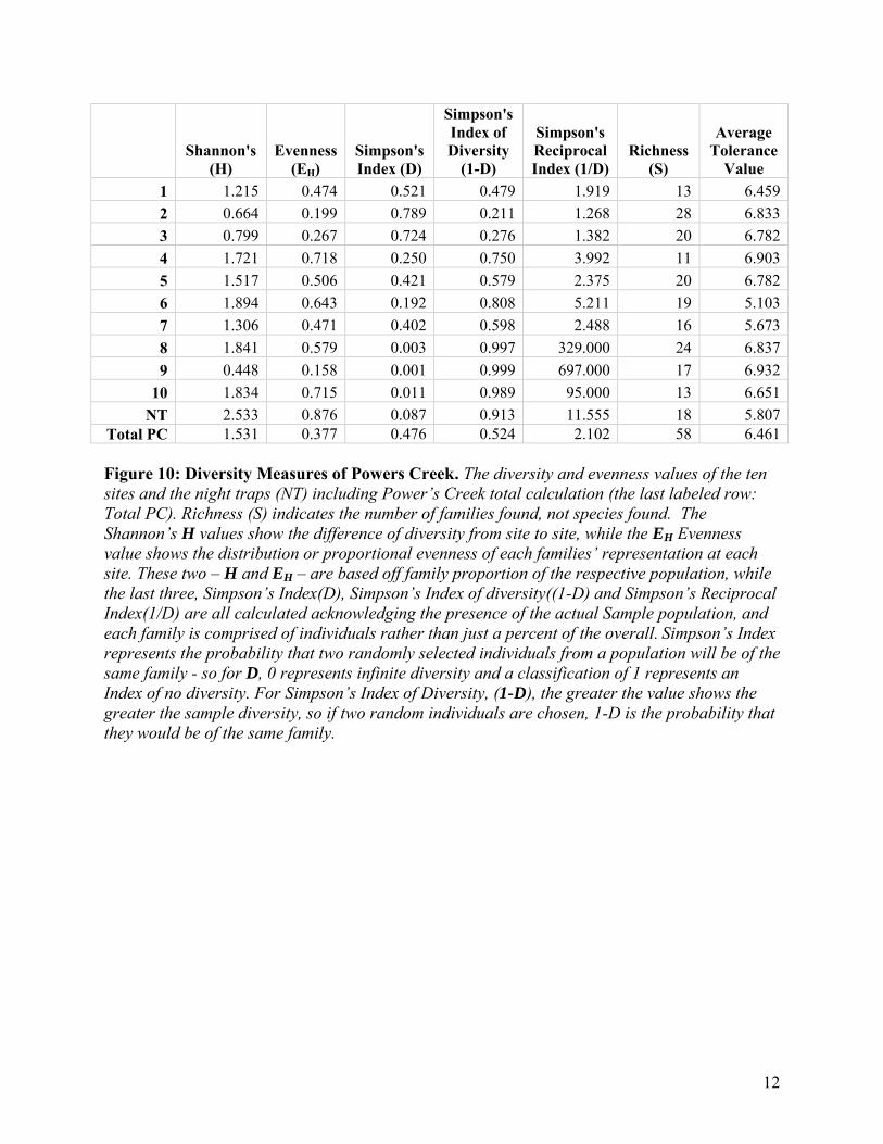
Total PC 1.531 0.377 0.476 0.524 2.102 58 6.461 Figure 10: Diversity Measures of Powers Creek. The diversity and evenness values of the ten sites and the night traps (NT) including Power’s Creek total calculation (the last labeled row: Total PC). Richness (S) indicates the number of families found, not species found. The Shannon’s H values show the difference of diversity from site to site, while the EH Evenness value shows the distribution or proportional evenness of each families’ representation at each site. These two – H and EH – are based off family proportion of the respective population, while the last three, Simpson’s Index(D), Simpson’s Index of diversity((1-D) and Simpson’s Reciprocal Index(1/D) are all calculated acknowledging the presence of the actual Sample population, and each family is comprised of individuals rather than just a percent of the overall. Simpson’s Index represents the probability that two randomly selected individuals from a population will be of the same family - so for D, 0 represents infinite diversity and a classification of 1 represents an Index of no diversity. For Simpson’s Index of Diversity, (1-D), the greater the value shows the greater the sample diversity, so if two random individuals are chosen, 1-D is the probability that they would be of the same family.

13

Figure 11: Substrate Collection: The numbers of individual insects found per substrate type at each site. The site’s available substrate affects the kind and the abundance of insect inhabitants.

Figure 12: Percent of Site's total count sampled from each substrate type. The overall percentage or proportions of each site’s collections are shown here, showing proportional significance of each substrate.

0

200

400

600

800

1000

1200

1400

1600

1 2 3 4 5 6 7 8 9 10Nu

mb

er

of

ind

ivid

ual

s co

llect

ed

an

d id

en

tifi

ed

Site

Data Collected at each Site with a Focus on Substrate Type

DROP TRAPS

DETRITUS

FLOATING VEG

EM VEG

BENTHIC

ROCK

0%

20%

40%

60%

80%

100%

1 2 3 4 5 6 7 8 9 10

Pe

rce

nta

ge o

f Sa

mp

le

Site

Percent of Sample Collected from Each Substrate

DROP TRAPS

DETRITUS

FLOATING VEG

EM VEG

BENTHIC

ROCK

14

Figure 13: The Average Tolerance Value of the Insects Collected at each Site. The Tolerance Value of an insect is low for less tolerant or more sensitive insects (specialists) and higher for more tolerant or less sensitive insects (generalists). (Not including the families Hebridae, Miridae, Noctuidae, and Ptilidae due to unknown tolerance value numbers.) (NT represents Night Traps)

Figure 14: The functional feeding groups of all specimens. Proportionality is shown to emphasize the aquatic insect's majority role as feeders and the importance of lower trophic levels that these insects belong to.

15

Figure 15: Distribution of Feeding Groups of the entire Power’s Creek Collection. The proportion of the feeding groups highlights the dominance of certain families that are in the Gathering Collectors Group. DISCUSSION

PHYSIOCHEMICAL PARAMETERS WATER ANALYSIS

Aquatic insect communities are determined by the abiotic parameters of the water in which they live. A number of these factors such as temperature, nutrient loads and pH were examined along Powers Creek to examine difference if any with respect to the insect communities. Figures 4 and 5 show the data for all water tests. Figure 4 displays the non-chemical tests (width, depth, turbidity, etc.) conducted at each site, while Figure 5 shows the chemical tests (pH, CO2, DO, etc.). As previously mentioned, non-chemical (Figure 4) sampling occurred twice; therefore the data displayed in in the figures is an average of the two sample sets. However, due to the poor conditions at site 4, some measurements were only able to be taken once, and therefore are not an average; these measurements in Figure 4 are marked with an asterisks (*). Though it was not in keeping with our intended methodology, all other chemical factors displayed in Figure 5 were sampled only once during the first sample set, due to lack of time and resources. While most of the measurements were similar between samples sets, others fluctuated greatly. The difference between sample set 1 and sample set 2 is assumed to be caused by natural changes in weather, such as rain and increase of heat over the summer months; all variables expected in an observational study. The averages of the two sample sets are displayed

83%

7% 6% 2%

1%

16

in order to create a better understanding of the creek’s structure (for raw data set see Appendix 7).

It was predicted that flow rate would be relatively low and depth would be shallow, given the initial walkthrough of the creek. Depth measurements ranged from 1.25-15 cm with an average of 6.68 cm. The creek was deepest at site 10, and shallowest at site 4. Flow rate had an average of 0.1327 m/sec; it never exceeded the measurement of 0.3333 m/sec at site 6, while the minimum flow rate was 0.0 m/s, which occurred at sites 4 and 5. Turbidity affects how much light can enter the water, which ultimately influences water temperature and what can grow and survive. Turbidity is caused by erosion and urban runoff, both of which were present during our initial walkthrough of Power’s Creek (EPA, 2014). Due to the amount of erosion around the stream, turbidity was predicted to be high. Turbidity had an average reading of 10.8 JTU, but fluctuated overall from 5.5-40 JTU. The clearest water occurred at site 1, while the highest turbidity was at Site 4. One of the two sample sets of turbidity measures at site 4 was unable to be collected due to the extreme shallowness of the water at time of sampling. Water temperature greatly affects what sort of organisms live in an area. Too hot or too cold temperatures not only directly affects an organism’s ability to survive, and but slight changes in temperature affects any chemical reactions taking place in the water, which could lead to creating unsuitable conditions (Senese, 2015). Temperature was expected to fluctuate throughout the creek. Temperature measurements ranged from 15.5-24.5oC, and the overall creek average was 19.66oC. Again, one of the two temperature samples from site 4 was unable to be obtained due to lack of water at the site at time of sampling, therefore the reading in Figure 4 for temperature is not an average between two sample sets, but is the reading from the single successful measurement.

High alkalinity and hardness were expected because of previously high readings and the calcium bicarbonate deposit creek source. Alkalinity and hardness did measure as high, though not directly at the spring source; the two measurements are directly compared in Figure 6. Alkalinity was highest at Site 5 at 468.64 (mg/L), and lowest at Site 7 at 204.87 (mg/L), with an average of 318.963 (mg/L). Hardness had an average of 466.8 (mg/L) with the highest value of 556 (mg/L) at Site 4, and lowest value of 356 (mg/L) at Site 7. Such high levels are considered normal as a result of the limestone bedrock through which the spring is sourced. However, alkalinity and hardness did not peak where the creek is spring-fed, at sites 1 and 2, which is where we predicted it to if water quality were a direct result of the spring. Fractured carbonate bedrock makes up the majority of Gratiot County; the consistently high alkalinity and hardness are more likely explained by the limestone bedrock throughout the property than as a direct result of the spring (Illinois State Geological Survey, 2016). There is an overall drop in the alkalinity and hardness levels after site 5, which can also be clearly observed in Figure 6. This may be caused by several variables; sites 1-5 and 6-10 were sampled in on two separate dates, and samples taken back to a lab at Loyola’s Lakeshore Campus. We attribute the difference between the sample sets to the rain which took place the night before samples for 6-10 were collected, the rainwater from which likely diluted the alkalinity and hardness within the sample. This decrease of alkalinity and hardness may also be partially due to the large pond which drains into the creek between site 5 and 6, which may dilute the water throughout the rest of the creek.

The pH affects how phosphorus and other chemicals are absorbed into the water and utilized by the organisms within it (USGS, 2016). Many aquatic organisms are held within a small pH threshold and therefore it was necessary to test. Due to Powers Creek’s expected high alkalinity and the direct correlation between alkalinity and pH, we predicted a high pH. The results of the pH tests did turn out to be high; which also corresponds with the results of the

17

water’s alkalinity and hardness tests. pH had an average value of 7.88, ranging from 7.2-8.2, lowest at site 5 and highest at sites 6 and 9. However, in contrast to the perceived pattern found in the alkalinity and hardness data where the levels dropped after site 5, the pH was fairly consistent, with a mode and median of 8 pH, and an average of 7.88 pH. There were no significant patterns to identify in this data set; the slight fluctuations are expected with many extraneous variables present along the creek.

DO is enriched by submerged aquatic plants and faster flowing water over rocks, roots, and other obstacles. Due to our initial observations of lack of aquatic plants in the creek, slow-flowing water, and history of eutrophication in the four ponds, we suspected lower ppm of DO in the creek. Moreover, CO2 is correlated to DO. The ratio of CO2 to DO should be relatively balanced, and an imbalance of either shows an unstable habitat. This is especially the case with high CO2, as a body of water with high CO2 is a key indicator of a distressed habitat (Great Lakes Lessons, 2016). High CO2 presence in water is often caused by eutrophication, which we assumed was high in this rural county with large farmlands, and therefore expected higher CO2 levels in the creek. CO2 levels also are an indicator of the ratio of respiring organisms versus photosynthesizers living in the ecosystem; high levels of CO2 indicate highly unbalanced ratio leaning towards respiring organisms. The values of each CO2 and DO test are compared directly in Figure 7. CO2 had an average value of 7.95 ppm, and DO an average of 4.58 ppm. CO2 ranged from 3 to 25 ppm, at sites 6 and 5 respectively. DO was highest at site 2 at 7.5 ppm, and lowest at site 5 at 1.6 ppm. Accurate DO sampling by the protocol of the test kit was not possible at site 4 due to shallowness, and therefore is marked in Figure 5 with a N/A, and is simply a gap in the Figure 7 trend line. The CO2 data is erratic at the first 5 sites, and therefore solid conclusions of the site based on this data cannot be made. However, there are characteristics of the data set which are worth noting. As mentioned before, there is an intrinsic connection between DO and CO2, and a balance between the two should be observed in a healthy habitat (Great Lakes Lessons, 2016). However, CO2 was particularly high at sites 2 and 5 which indicate a distressed habitat. This result is unexpected at site 2 as it has one of the higher flow-rates and the habitat contains large rocks that the water flows over and around. On the other hand, high CO2 at site 5 makes a great deal of sense given its habitat conditions. Both sites 4 and 5 are drainage ditches that catch runoff from the fields on either side; the water is predominantly stagnant and experiences direct sun exposure. These conditions and the result from site 5 then make the reading at site 4 seem uncharacteristically low. At sites 6-10, a balanced trend between DO and CO2 is observed. This too shows that this data set especially has many inconsistencies which prevent us from drawing conclusions upon the results.

Phosphorus and nitrogen are natural nutrients essential for plant growth; they are found in manure and commercial fertilizer, and used on farms, therefore we expected phosphorus and nitrogen levels to be slightly higher due to the agricultural land use in the area (USGS, 2016). However, nitrates and phosphates were both low and did not have much notable fluctuation or correlation. Nitrate measured its lowest values of 0.5 (ppm) at Sites 4, 5, 6, and 7; the highest value was 1.5 (ppm) at Site 1, and was an average of 0.87 (ppm) overall. Phosphate ranged from 0 (ppm) at Sites 1, 3, 6, 7, 8, and 10, to 0.2 (ppm) at Sites 4 and 5. These levels were normal and expected. Lower levels of nitrogen and phosphate may indicate that the agricultural runoff in the area does not affect LUREC’s portion of Power’s Creek very much, and not nearly as much as we predicted prior to this analysis.

18

SOIL ANALYSIS The soil data is displayed in Figure 8. The pH was consistent, and merely fluctuated

between 8 and 8.2; the median and average reading was 8.2, which was recorded at all sites except for sites 2 and 4. The nitrogen levels were also fairly consistent, with outlier of site 8. The reading at most sites was Trace (sites 1, 2, 4, 5, 6, and 10), and was lowest at sites 3 and 7 with a reading of None. In Figure 8, site 8 is described as having a “High/Low” reading because it was tested twice: high was the first result, low was the second. Because the first reading was so uncharacteristic of other sites, we wanted to retest it. Low was the second result, which is much more in line with the rest of the results. This outlier was probably due to test kit error. AQUATIC INSECTS COMMUNITY

A range of 13 to 31 families of aquatic and semiaquatic insects were identified at each site. Strictly aquatic insects have site richness values ranging from 13 to 28 families. The three sites with the highest richness are sites 2 with 28 families, Site 8 with 26 families and Site 5 with 23 families (Figure 9). There is a positive correlation between the individual site’s richness and the number of families found between the two rounds. Sample Set 2 resulted in higher richness of families found at the sites when compared to the first sample set. This is shown in seven out of the ten sites with more families recorded in the second round of sampling, (see dates Appendix 2).

Of the total families collected, we saw the highest numbers in the Chironomidae (midges), Simulidae (Black Flies), and Aphididae(Aphids) (see Appendix 6 and Appendix 9). Aphididae, was collected as a semiaquatic insect because of its presence on emergent and floating vegetation as well as other terrestrially growing vegetation that may become submerged from time to time. We will leave Aphididae presence out of discussion, but note the numbers in the Appendix 6 for any reference for future studies. So of the 65 families found and recorded, only 58 of them will be treated as aquatic insects for the purpose of discussion, omitting Bibionidae (1), Aphididae (721), Cicadellidae (14), Thripidae (24), Ichneumonidae (1), Coccinelidae (11), and Platygastridae (2) which make up 774 or 14.5% of original total count (see Appendix 6). This lowers the total count from 5316 to 4554 individuals within 58 families – lowered from 65 families – as our new respective total. We also lose two orders – Hymenoptera and Thysanoptera – when lowering the total aquatic orders down to 8. BETWEEN SAMPLE SETS

The second sample set yielded significantly higher individual counts than sample set one. In the first round of testing, the highest counts seen at any of the sites was 620 individuals in the Chironomidae (midge). In the second round of testing, the highest number count for the entire project was reached with 1204 individuals identified to the family Chironomidae at site 2 and another astonishing number of 635 at site 9. This is an example of the effect of the time of year yielding higher numbers (see Appendix 2).

Elmidae (riffle beetles), Pychopteridae (phantom crane flies), and Ceratopogonidae (crane flies) all were seen to have high numbers as well. The beetle family Elmidae, a generalist, was found in quite high numbers. This family was quite surprising, because the first sample set found many larval stages of this beetle, while the second sample set found more adult stages of this beetle. This larvae is adapted for low oxygen environments and have a fan like structure at the apex of their abdomen to increase surface area for oxygen diffusion (see Appendix 10). This

19

larva was normally found in detritus, which makes sense with its generalistic feeding preferences and for the low oxygen adaptations it possess. The Pychopteridae (phantom crane flies) possess this feature as well. The Tipulids (crane flies) and Pychopterids (phantom crane flies) are known to emerge midway through the summer, these are found at sites with low DO concentrations, and came in higher numbers towards the second round of collections. NIGHT TRAP COLLECTIONS

Night traps collected 70 individuals from 18 different families (see Appendix 9). Of the total count, night traps accounted for only 2% of the total specimen count, leading to less inquiry about the flying adult aquatic insects than we would have hoped. This is because emergence for many aquatic insects is in the earlier summer months. For most of the orders, the percent of the total count of Power’s Creek collected via night traps was less than 10%, but in the case of Ephemeroptera 2 of 9 individuals were collected from the night trap collection. These 2 were collected at Night Trap B, [between 7:47 and 9:38 pm on July 14].

Night traps had a relatively low tolerance value of 5.81, being the third lowest when compared along with the ten sites, the average tolerance value of the creek being 6.46 (see Figure 13). Lower tolerant insects with different life stages, such as those caught in the night traps, depend on stability of the ecosystem for each life stage, especially after emergence. Therefore, it is of good use to use this tolerance test to see the aerial community’s tolerance to disruption. Night trap data had a Simpson’s Index of Diversity value among the top three as compared with the ten sites with a value of 0.913 and it had the highest evenness value found among the sites. DROP TRAP COLLECTIONS

Drop Traps accounted for 83 total specimens from 7 different orders, 14 different families and this accounted for 2% of the specimen count (see Appendix 11). The drop trap data came from a collection over four days. The irregularities in weather and conditions between the days of drop trap collections could be an extraneous variable. The time of day and therefore lack of shade is an indicator as to why the lowest representatives for this sample type are pupae, because most drop traps were put out in the middle hours of the day. This testing technique was performed to collect the emerging pupae and contrary to prediction, many adult Dipterans were collected.

However, drop traps did prove to be quite useful for the collection of the semi-aquatic Collembolans, commonly known as springtails or snow fleas. We found 3 families of Collembolans in the drop traps, which was 48% of the total drop trap data, with 50 individual Collembola collected. This Hexapod relative was included in the aquatic insect count because of their similar nature to aquatic insects. Their occurrence indicates the quality of the soil at each location with higher collembolan numbers indicating a higher water content and overall moisture retention ability of the soil.

Also, some Hymenopterans (family Platygastridae) were discovered in the drop traps. Their presence indicates the connection to their host, an aquatic Lepidopteran pupa which they parasitize. This family of Lepidoptera, Crambidae, is usually hard to collect with the collection methods we employed. The larvae usually are found within the xylem of aquatic plants in which they feed and to conserve water. In this study, 11 Crambid specimens were identified and 10 of them were larva. Nine of the larvae found were collected from emergent plant substrates. The two platygastrids found in the drop traps were wingless, indicating that these specimens are ovipositing females, and female parasites in this family are known to protect and stay near their

20

host to ensure their egg’s incubation safety (Johnson, 2004). The moth Crambidae was also found at other sites, and due to the drop traps’ data, we can see interspecific relationships among these families of insects. SUBSTRATE ANALYSIS

Detritus was the substrate that had the most insect individuals found within its sample type. This substrate was found at most sites, but rocks were only found at two, and they were the next highest counts. The 2nd and the 6th site were the only sites where rock substrates were present. When referencing Figure 11 and Figure 12, the rock samples are responsible for the highest data collections. According to Merrit et.al 2008, aquatic insects are found in very high numbers in areas of a quickly moving stream that have rocky substrates so insects can cling onto. These sites are especially important for pupation. A stream bed containing large rocks is proven to be important for the colonial pupating Chironomidae and Simulidae. The time of year is also indicative of confirming the high numbers, for June-August will see dwindling, but still quite high numbers of these dipteran communities that are reliant on these loose, rocky bottoms.

At Site 2, aquatic insects from the rock substrate samples were an astonishing 90% (944/1050) of the whole benthic sample while only 10% (106/1050) came from the sampling of the creek bed. Of the 8 families found in this site's benthic sample, 4 were only found on rock substrates.

At Site 6, the individuals collected from the rock substrate accounted for 80% (320/398) of the of the combined benthic sample. There were 14 families represented in the overall 398 count. Site 6 was a well-shaded sandy-bottomed site with detritus. Site 6 also had more “even” counts for a diverse range of families (see Figure 10), and had the most specialist or low tolerant valued-families (see Figure 13). Other than the relatively high numbers of Chironomidae that was also found at the other sites, Site 6 had the highest count of Simulidae, Elmidae, and relatively high numbers of Hydropsychidae (Net-Spinning Caddisflies). Simulidae saw its highest count at Site 6 with 192 specimens identified, mostly in the pupal stage.

FEEDING GROUP ANALYSIS

Figure 14 and Figure 15 highlights the majority of the feeding groups (see references to Appendix 8 for background of FFG and Tolerance value of each family). Predators eat on live prey; Collectors are plait into two groups: Gatherers that collects and feed on course particulate organic matter (CPOM), and Filterers that collects and feed on fine particulate organic matter (FPOM). Scrapers eat algae and microbes stuck to surfaces. Shedders feed on living and dead plant vascular matter such as wood. Our results showed that Collector/Gatherers are the majority functional feeding group in these samples, with an astounding 83% of the specimens collected to be in this group. Not surprising, Filtering Collectors followed with 7%, predators with 6%, Shredders with 2%, and Scrapers accounted for the remaining 1% of the sample. Functional Feeding Groups were recorded at analyzed for patterns at each of the ten sites, (see Appendix 12). The sample data was used to find P/R ratios that predict each site’s heterotrophic or autotrophic state. All the sites in each sampling round were found to be so strongly heterotrophic (or reliant on material and energy from outside of the stream) that the most numbers were near zero. This could be due to the lack of scrapers that were found.

The CPOM to FPOM ratios were calculated for each site and all were each found to have very poor links with the riparian zone (see Panock, 2016). However since shredders were nearly absent in all sites samples, vegetation found in or around the sample sites in Power’s Creek is

21

quite inefficient as a food source for shredders. To have a functional riparian zone, there needs to be more shredders in the collection.

Site 6 was the only site to show a healthy amount of suspended loading of FPOM, probably due to this site having the highest number of Hydropsychidae (Common Net Spinning Caddisflies) with a count of 84 individuals. The Hydropsychidae are important Filtering Collectors and their dominance allows healthy loading of FPOM. Their abundance here at site 6 shows that the healthy amount of suspended FPOM is being turned over to benthic FPOM sufficiently.

Channel Habitat Stability was calculated and found to be sub-adequate with results all far below the threshold at all sites except Site 6. Only at this site was there an adequate array of stable substrates for a diverse amount of feeding groups to be present (see Appendix 12) Conclusion: While Powers Creek provides habitat for a variety of organism, its current conditions does not support a diverse variety of aquatic organisms that would likely otherwise be present. Fluctuations in physiochemical factors along LUREC’s property and the apparently limited variety of plants are too great to provide a well-supported habitat for a biotic community. There are many future implications of this study. Ecological studies usually take place over several years; therefore this study could serve as a starting point for a long-term observation of Powers Creek as Loyola continues with restoration work. A parallel study could be conducted at the conclusion of restoration in order to assess the restoration's effectiveness in improving habitat quality. The aquatic insect community should increase with greater plant variety increases once restoration is completed and the hydrology of the area improved. Acknowledgements: Special thanks are extended to Dr. Roberta Lammers-Campbell for her assistance in plant identification and various textual resources. Thanks to Samantha Panock for assistance with transect and photographing each site for reference. In particular, thanks to the wonderful staff at LUREC. Financial support was provided as a biodiversity internship by the Institute of Environmental Sustainability, Loyola University Chicago.

22

REFERENCES Aquatic Life Ambient Water Quality Criteria for Ammonia - Freshwater. Washington, D.C.:

U.S. Environmental Protection Agency, Office of Water, Office of Science and

Technology, 2013. Aquatic Life Ambient Water Quality Criteria For Ammonia –

Freshwater 2013. Environmental Protection Agency.

Ceballos, G. et alt. Accelerated modern human–induced species losses: Entering the sixth mass

extinction. 2015. Science Advances. 1:5.

Eaton, A.D., Clesceri, L.S., Greenberg, A.E., Rice, E.W., 2005. Standard Methods for the

Examination of Water andWastewater, twenty-first ed. American Public Health

Association. United Book Press Inc, Baltimore, Maryland.

"Issues in Ecology." Bulletin of the Ecological Society of America 86.4 (2005): 249-50.

"Illinois State Geological Survey." Illinois State Geological Survey Geologic Setting in

McHenry County, Illinois | ISGS. Prairie Research Institute, 2017. Web. 01 Mar. 2017.

Johnson, N. F. "Platygastroidea: Biology." Platygastroidea: Biology. National Science

Foundation, 17 Jan. 2004. Web. 02 Feb. 2017.

"Lessons and Data Sets." Teaching Great Lakes Science, n.d. Web. 01 Mar. 2017.

Merritt, R.W., K.W. Cummins, and M.B. Berg, eds. 2008. An Introduction to the Aquatic Insects

of North America. 4th Ed., Kendall/Hunt Publishing Co., Dubuque, Iowa.

Olmedo, G. and S. Mitten 2015. Environmental Changes of Three Calcareous Ponds at Loyola

Retreat and Ecology Campus.

http://luc.edu/media/lucedu/retreatcampus/pdfs/Environmental%20changes%20in%20three

%20Calcareous%20Ponds.pdf

Pacholski, C., S. Keyport, J. Gasior and S. Mitten 2014. Ecosystem Profile Assessment of

Biodiversity at Loyola University Retreat and Ecology Campus.

http://luc.edu/media/lucedu/retreatcampus/pdfs/Ecosystem%20Profile%20Assessment%20o

f%20Biodiversity%20at%20LUREC%20final%202.pdf

Panock, S. 2017 Aquatic and Shoreline Terrestrial Plant Composition with Floristic Quality

Index of Powers Creek at Loyola University Retreat and Ecology Campus,

McHenry County, IL 2016

Perlman, H. PH -- Water Properties. USGS. USGS Water-Science School, 2016.

Perlman, H. Phosphorus and Water. USGS. USGS Water-Science School, 2016.

23

Perez, E. and S. Mitten. 2012 Avian Species Structure at Loyola University Retreat and Ecology

Campus during the 2012 Summer Breeding Season.

http://www.luc.edu/media/lucedu/retreatcampus/pdfs/Avian%20Species%20Structure%20at%20

Loyola%20University%20Retreat%20and%20Ecology%20Campus%20Final-1.pdf

Rockstrom et alt. Planetary Boundaries: Exploring the Safe Operating Space for Humanity.

2009. Ecology and Society. (14:2. 32.)

Senese, F. Chemistry Online: FAQ: Solutions: Why Does the Solubility of Gases Usually

Increase as Temperature Goes Down? N.p., 2010. Web. 01 Mar. 2017.

Warner, K. L., P. J. Terrio, T. D. Straub, D. Roseboom, and G. P. Johnson. Real-time

Continuous Nitrate Monitoring in Illinois in 2013. Fact Sheet (2013): Water Quality

Association, 2014. Web.

The Watershed Management Plan. The Watershed Project Management Guide (2016): Fox River

Ecosystem. CMAP, Mar. 2016. Web. 17 Aug. 2016.

24

APPENDIX

Site Location

1 N 42.29010, W -88.36797

2 N 42.28991, W -88.36716

3 N 42.28948, W -88.36667

4 N 42.28964, W -88.36587

5 N 42.28958, W -88.36502

6 N 42.28956, W -88.36393

7 N 42.28956, W -88.36304

8 N 42.28955, W -88.36217

9 N 42.28957, W -88.36136

10 N 42.28938, W -88.36062

Appendix 1: The location of each site setup, shown by each site’s coordinates as seen in Figure 3’s aerial photo.

Appendix 2: Sampling Dates: used to lay out the time range of the data collected, and explain any population differences seen between samples taken.

25

Night Trap Number

Location

1 N 42.28978, W -88.36684

2 N 42.28956, W -88.36393

3 N 42.28955, W -88.36217

Appendix 3: The geographic locations of the night traps (in degrees).

Appendix 4: Night Trap Setup. Night trap set up the day of the Night traps, assessing placement for best tray placement and setting up the pole angle and placement.

Orders Sample 1 Sample 2 Drop Traps Night Traps Total Diptera 944 2634 29 38 3645 Collembola* 88 28 40 7 163 Hemiptera 623 273 8 13 917 Coleoptera 135 191 1 21 348 Trichoptera 145 39 0 1 185 Thysanoptera* 5 16 2 1 24 Hymenoptera* 1 0 2 0 3 Lepidoptera* 2 8 1 1 12 Ephemeroptera 6 1 0 2 9 Odonata 3 7 0 0 10 1952 3197 83 84 5316 Appendix 5: The aquatic and semi-aquatic total counts of individuals within each order at Power's creek from each sample set. All together making the summer's count of insects to be 5316 of aquatic and semi aquatic insects. (* Semi-aquatic orders marked.)

26

Order Family 1 2 3 4 5 6 7 8 9 10 NT Sum Diptera Bibionidae 0 0 0 0 0 0 0 0 1 0 0 1 Hemiptera Aphididae 0 162 4 133 161 13 37 199 5 5 2 721 Hemiptera Cicadellidae 0 0 1 0 0 1 0 1 0 0 11 14 Coleoptera Coccinellidae 0 0 0 3 3 0 0 1 0 4 0 11 Thysanoptera Thripidae 1 1 5 1 2 0 0 0 6 7 1 24 Hymenoptera Ichneumonidae 0 0 1 0 0 0 0 0 0 0 0 1 Hymenoptera Platygastridae 0 1 1 0 0 0 0 0 0 0 0 2

774 Appendix 6: The total counts of the semi-aquatic representatives omitted from aquatic discussion. The 774 individuals in this category would make up around 14.7% of all insect data collected. *NT represents Night Traps. Test Number

Width (cm)

Flow Rate (m/sec)

Temp (◦C)

Turbidity (JTU)

1.1 51 0.167 15 8 1.2 35 0.146 17 3 2.1 124 0.125 14 13 2.2 133 0.151 17 20 3.1 170 0.09 17 7 3.2 140 0.111 19 5 4.1 58 0 18 N/A 4.2 70 0 N/A N/A 5.1 110 0 18 10 5.2 90 0 19 30 6.1 77 0.33 23.5 8 6.2 66 0.42 24 10 7.1 110 0.25 24 10 7.2 113 0.247 25 4 8.1 140 0.04 21 10 8.2 143 0.149 22 20 9.1 65 0.11 19 10 9.2 95 0.083 22 10 10.1 107 0.105 17 12 10.2 90 0.13 22 5 Avg. 99.35 6.675 0.1327 19.65789474 Appendix 7: Raw data for water samples. All of the data which was taken in two sets of sampling. “Test Number” column indicates the site, and if it was sample set 1 or 2; for example, Test Number “8.2” means site 8, sample set 2.

27

Family Common Name

Tolerance Value

Functional Feeding Group

Aeshnidae Darner Flies 3 P Athericidae Water Snipe Flies 2 P Baetidae Small Minnow Mayfly 4 CG Calopterygidae Broadwinged Damselflies 5 P Carabidae Ground Beetles 4 P Cecidomyiidae Gall Midges 0.2 SH Ceratopogonidae Biting Midges 6 P Chironomidae Midges 7 CG Chrysomelidae Aquatic Leaf Beetles 5 SH Coenagrionidae Narrow-winged Damselflies 9 P Corixidae Water Boatmen 9 P Crambidae Snout moth 2.7 SH Culicidae Mosquitoes 8 CG Curculionidae Water Weevil 5 SH Dixidae Dixid Midges 1 CG Dolichopodidae Aquatic Longlegged Flies 4 P Dryopidae Long-toed Water Beetles 3.2 CG Dytiscidae Predaceous Diving Beetles 5 P Elmidae Riffle Beetles 3 CG Empididae Aquatic Dance Flies 3.5 P Entomobryidae Entomobryids 10 CG Ephydridae Shore Flies 6 CG Georissidae Mud Loving Beetles 5 P Gerridae Water Striders 5 P Gyrinidae Whirligig Beetles 4 P

Haliplidae Crawling Water Beetle 7 FC Hydrophilidae Water Scavenger Beetles 5 CG Hydropsychidae Common Netspinners 4 FC Hydroptilidae Micro Caddisflies 4 SC Hydroscaphidae Skiff Beetle 7 SC Lampyridae Fireflies 6 P Libellulidae Common Skimmers 7 P Limnephilidae Northern Casemakers 4 SH Metretopodidae Cleft Footed Mayfly 2 CG Microveliidae Short-Legged Water Striders 5 P Muscidae House Fly 6 P Nepidae Water Scorpions 8 P Pelecorhynchidae Rubber Flies 3 P Phoridae Humpbacked Flies 7 P Poduridae Podurid Springtails 10 CG

28

Psephenidae Water-penny beetle 4 SC Psychodidae Moth Flies 10 CG Ptilodactylidae Toe-winged Beetles 3 SH Ptychopteridae Phantom Crane Flies 7 CG Scathophagidae Dung Flies 6 SH Sciomyzidae Marsh Flies 6 P Scirtidae Marsh Beetles 7 SH Simuliidae Black Flies 6 FC Sminthuridae Sminthurid Springtails 10 CG Stratiomyidae Aquatic Soldier Flies 8 CG Tabanidae Horse and Deer Flies 4.6 P Thaulmaleidae Solitary Midges 8.8 - Tipulidae Crane Flies 3 SH Veliidae Short Legged Striders 6 P

Feeding Group/Trophic Relationship

CG = Collector/Gatherer CF=Collector/Filterer

SC = Scraper SH = shredder PR = predator

Appendix 8: The Common Name, Tolerance Values, and Functional Feeding Group of each of the aquatic insect families found in the study. Below the chart is the key for the abbreviated terms.

1 2 3 4 5 6 7 8 9 10 NT Total Aeshnidae 0 0 0 0 0 0 0 3 1 0 0 4 Athericidae 6 0 0 0 0 0 0 0 0 0 0 6 Baetidae 0 0 0 0 0 4 0 1 0 0 2 7 Calopterygidae 0 0 0 0 0 2 2 0 0 0 0 4 Carabidae 0 0 0 0 0 0 0 1 0 0 0 1 Cecidomyiidae 2 0 0 0 6 8 0 0 0 0 0 16 Ceratopogonidae 8 7 16 0 4 6 12 23 8 9 0 93 Chironomidae 158 1310 316 12 144 162 161 152 645 46 3 3109 Chrysomelidae 0 0 0 0 0 0 0 0 1 0 0 1 Coenagrionidae 0 0 0 0 1 0 0 0 0 0 0 1 Corixidae 0 0 0 0 0 0 0 0 2 0 0 2 Crambidae 0 1 0 5 0 0 1 3 0 0 1 11 Culicidae 0 0 1 0 0 1 0 1 0 0 0 3 Curculionidae 0 1 0 0 1 0 0 1 1 0 0 4

29

Dixidae 0 0 4 0 0 0 0 1 0 0 0 5 Dolichopodidae 0 2 0 0 0 0 1 0 0 0 6 9 Dryopidae 0 0 1 0 0 0 0 0 0 0 0 1 Dytiscidae 0 1 1 0 0 0 0 0 0 0 0 2 Elmidae 0 26 7 0 2 162 80 28 9 0 0 314 Empididae 0 6 4 0 2 26 7 6 1 3 1 56 Entomobryidae 0 0 2 0 0 0 0 2 0 0 0 4 Ephydridae 0 3 1 1 1 0 1 0 0 2 0 9 Georissidae 0 0 0 0 1 0 0 0 0 0 0 1 Gerridae 0 3 0 0 0 3 4 8 8 11 0 37 Gyrinidae 0 1 2 0 0 0 0 0 0 0 0 3 Haliplidae 0 0 0 0 1 0 0 0 0 0 0 1 Hebridae 0 13 0 0 0 0 0 0 0 0 0 13 Hydrophilidae 0 2 0 2 9 1 0 2 0 2 11 29 Hydropsychidae 19 15 0 0 0 82 1 0 0 0 1 118 Hydroptilidae 0 0 1 0 0 42 0 1 1 0 0 45 Hydroscaphidae 0 1 0 0 0 0 0 0 0 0 0 1 Lampyridae 0 0 0 0 1 0 0 0 0 0 1 2 Libuellidae 0 0 1 0 0 0 0 0 0 0 0 1 Limnephilidae 7 26 0 0 0 0 0 1 0 1 0 35 Metretopodidae 0 0 0 0 0 2 1 0 0 0 0 3 Microveliidae 0 0 0 0 0 1 0 0 0 0 0 1 Miridae 0 0 1 0 0 0 0 0 0 0 0 1 Muscidae 0 5 0 2 0 1 0 0 0 0 1 9 Nepidae 0 0 0 0 0 0 1 0 0 0 0 1 Noctuidae 0 0 0 0 1 0 0 0 0 0 0 1 Pelecorhynchidae 0 0 0 0 0 0 0 1 0 0 0 1 Phoridae 0 6 1 0 0 0 0 0 0 0 0 7 Poduridae 6 4 5 9 20 17 4 69 7 7 5 153 Psephenidae 0 0 0 0 0 0 0 0 0 1 0 1 Psychodidae 1 14 0 0 0 0 0 1 0 0 3 19 Ptiliidae 0 0 0 0 0 0 0 0 1 0 9 10 Ptilodactylidae 0 0 0 0 1 0 0 0 0 0 0 1 Ptychopteridae 2 2 0 29 17 0 3 0 0 5 2 60 Scathophagidae 0 1 0 0 0 0 0 2 0 0 0 3 Sciomyzidae 0 3 0 0 0 0 0 2 1 1 11 18 Scirtidae 0 0 0 1 0 0 0 0 0 0 0 1 Simulidae 2 0 2 0 0 192 1 0 0 0 2 199 Sminthuridae 0 2 0 0 0 0 0 0 1 2 2 7 Stratiomyidae 5 8 3 1 3 0 0 0 7 0 1 28 Tabanidae 0 1 0 2 0 0 0 2 0 0 0 5 Thalmaleidae 0 0 0 0 1 0 0 0 0 0 0 1 Tipulidae 3 1 1 0 6 2 0 6 1 0 8 28

30

Veliidae 2 11 2 1 4 2 4 13 3 6 0 48 Total 221 1476 372 65 226 716 284 330 698 96 70 4554

Appendix 9: These are the total counts for each site. Including the combined sample sets 1 and 2, drop trap data, and the Night Traps(the three locations combined). These are the fully aquatic species which are made up of 58 families and 4554 individual specimens.* NT stands for Night Traps.

Appendix 10: Elmidae (left) and Phychopteridae (right) Larvae. The two most common larvae families found. Total Families Total Specimens Diptera 5 29 Collembola* 3 40 Hemiptera 2 8 Coleoptera 1 1 Thysanoptera* 1 2 Hymneoptera* 1 2 Lepidoptera* 1 1 Drop Trop Total 14 83 Appendix 11: The Drop Trap Data. This shows the numbers of individuals found in each order and the number of families found in each order. Seven total were represented in the drop trap data. (* refers to a semi-aquatic representative)

31

Site Ecosystem Parameter

FFG Ratio Threshold Interpretation

1 P/R 0.00 > 0.75 Scraper Underrepresented 2 P/R 0.00 > 0.75 Scraper Underrepresented 3 P/R 0.00 > 0.75 Scraper Underrepresented 4 P/R 0.00 > 0.75 Scraper Underrepresented 5 P/R 0.00 > 0.75 Scraper Underrepresented 6 P/R 0.07 > 0.75 Strongly heterotrophic 7 P/R 0.00 > 0.75 Scraper Underrepresented 8 P/R 0.00 > 0.75 Scraper Underrepresented 9 P/R 0.01 > 0.75 Strongly heterotrophic

10 P/R 0.02 > 0.75 Very strongly heterotrophic Total PC: P/R 0.01 > 0.75 Scraper Underrepresented

1 CPOM/FPOM 6% > 0.25 Poor Shredder Link with Riparian 2 CPOM/FPOM 2% > 0.25 Very poor shredder link with riparian 3 CPOM/FPOM 1% > 0.25 Shredders Underrepresented 4 CPOM/FPOM 13% > 0.25 Poor Shredder Link with Riparian 5 CPOM/FPOM 8% > 0.25 Shredders Underrepresented 6 CPOM/FPOM 2% > 0.25 Very poor shredder link with riparian 7 CPOM/FPOM 0% > 0.25 Shredders Underrepresented 8 CPOM/FPOM 5% > 0.25 Very poor shredder link with riparian 9 CPOM/FPOM 0% > 0.25 Shredders Underrepresented

10 CPOM/FPOM 2% > 0.25 Shredders Underrepresented Total PC: CPOM/FPOM 2% > 0.25 Very poor shredder link with riparian

1 TFPOM/BFPOM 0.13 >0.5 Reduced Suspended Loading of FPOM 2 TFPOM/BFPOM 0.01 >0.5 Very Light Suspended Load 3 TFPOM/BFPOM 0.01 >0.5 Very Light Suspended Load 4 TFPOM/BFPOM 0.00 >0.5 Very Light Suspended Load 5 TFPOM/BFPOM 0.01 >0.5 Very Light Suspended Load 6 TFPOM/BFPOM 0.79 >0.5 Stable Substrates Abundant 7 TFPOM/BFPOM 0.01 >0.5 Very Light Suspended Load 8 TFPOM/BFPOM 0.00 >0.5 Very Light Suspended Load

9 TFPOM/BFPOM 0.00 >0.5 Very Light Suspended Load 10 TFPOM/BFPOM 0.00 >0.5 Very Light Suspended Load

Total PC: TFPOM/BFPOM 0.09 >0.5 Light Suspended Load

1 Channel Stability 0.12 >0.5 Stable Substrates Adequate

2 Channel Stability 0.01 >0.5 Stable substrates Sub-Adequate

32

3 Channel Stability 0.01 >0.5 Stable substrates Sub-Adequate

4 Channel Stability 0.00 >0.5 Stable substrates Sub-Adequate 5 Channel Stability 0.00 >0.5 Stable substrates Sub-Adequate 6 Channel Stability 0.89 >0.5 Stable Substrates Abundant 7 Channel Stability 0.01 >0.5 Stable substrates Sub-Adequate 8 Channel Stability 0.00 >0.5 Stable substrates Sub-Adequate 9 Channel Stability 0.01 >0.5 Stable substrates Sub-Adequate

10 Channel Stability 0.02 >0.5 Stable substrates Sub-Adequate Total PC: Channel Stability 0.10 >0.5 Stable Substrates Adequate

Appendix 12: Functional Feeding Group (FFG) Analysis of the site’s sample rounds at Power’s Creek. The P/R [=(Scrapers)/ (Total Collectors + Shredders)]; CPOM/FPOM [=(Shredders/Total Collectors)]; TFPOM/BFPOM [=(Filtering Collectors/Gathering Collectors)]; and Channel Habitat Stability [=(Scrapers + Filtering Collectors)/(Gathering Collectors + Shredders)].