the aplicacion of traffic appraisal to trunk roads shemes

November 1997

DESIGN MANUAL FOR ROADS AND BRIDGES

VOLUME 12 TRAFFIC APPRAISAL OFROADS SCHEMES

SECTION 1 TRAFFIC APPRAISALMANUAL

PART 1

THE APPLICATION OF TRAFFICAPPRAISAL TO TRUNK ROADSSCHEMES

AMENDMENT NO. 1

SUMMARY

These are consequential amendments to the TrafficAppraisal Manual arising from the publication of theDesign Manual for Roads and Bridges, Volume 12,Section 2, Part 3 - The National Trip End Model.

INSTRUCTIONS FOR USE

1. Remove existing contents page from Volume 12dated February 1997 and insert page datedNovember 1997.

2. Insert the replacement pages listed on theamendment sheet (Amendment no. 1), remove thecorresponding existing pages which aresuperseded by this amendment.

3. Archive this sheet as appropriate

Note: A quarterly index with a full set of VolumeContents Pages is available separately from theStationery Office Ltd.


May 1996


VOLUME 12 TRAFFI C APPRAISALOF ROADS SCHEMES

SECTION 1 TRAFFI C APPRAISALMANUAL

PART 1

THE APPLIC ATIO N OF TRAFFICAPPRAISAL TO TRUNK ROADSCHEMES

SUMMA RY

The Department of Transport Traffic Appraisal Manual(TAM) sets out the recommended practice for theappraisal of trunk roads schemes. This documentintroduces the TAM to the DMRB as Volume 12. DMRB12.1.1 is composed of two parts: an introduction to theTAM which specifies which parts of the August 1991reprint of the TAM are to be retained and the Manualitself, described as an Annex to the Introduction .

INSTRUCTIONS FOR USE

This is a new document to be incorporated into theManual.

1. Insert DMRB 12.1.1 into Volume 12 atSection 1 in Binder 12.

2. Remove the parts of the existing TAM whichhave been withdrawn. Check that the remainingsections are dated August 1991 and then insert inBinder 12 after DMRB 12.1.1.

3 Archive this sheet as appropriate.

Note:

A binder for this Volume (12) and a full set of VolumeContents Pages are available separately from HMSO. Areprint of the August 1991 edition of the TAM is alsoavailable separately from HMSO.

November 1997


VOLUME 12 - TRAFFIC APPRAISAL OF ROADS SCHEMES

Section 1 Traffic Appraisal Manual

Part 1 The Application of Traffic Appraisal to Trunk Road Schemes

VOLUME 12a (continuation binder)

Section 2 Traffic Appraisal Advice

Part 1 Traffic Appraisal in Urban Areas

Part 2 Induced Traffic Appraisal

Part 3 The National Trip End Model

The application of traffic appraisalto trunk road schemes

THE HIGHWAYS AGENCY

THE SCOTTISH OFFICE DEVELOPMENT DEPARTMENT

THE WELSH OFFICEY SWYDDFA GYMREIG

THE DEPARTMENT OF THE ENVIRONMENT FORNORTHERN IRELAND


Summary: These amendments to the Traffic Appraisal Manual arise from thepublication of the Design Manual for Roads and Bridges, Volume 12,Section 2, Part 3 -The National Trip End Model

IncorporatingAmendment no. 1dated November

1997

Volume 12 Section 1Part 1

November 1997

Traffic Appraisal ManualRegistration of Amendments

REGISTRATION OF AMENDMENTS

Amendment Page No Initials & Amendment Page No Initials &No Date of No Date of

incorporation incorporationof ofamendments amendments

One Part 1replace:

Nov header page1997

Part 1replace:1/1 to 1/6

Part 1 Annex

remove:all of chapter 4

insert:“withdrawn” header page

Part 1 Annex

remove:all of chapter 7

insert:“withdrawn” header page

Part 1 Annex

replace:chapter 12 header page12/3, 12/412/13, 12/14

Part 1 Annex

remove:Data Appendix Dl

Part 1 Annexreplace:Data Appendicesheader page

Volume 12 Section 1Part 1

May 1996

Registration of Amendments

REGISTRATION OF AMENDMENTS

Amend Page No Signature & Date of Amend Page No Signature & Date ofNo incorporation of No incorporation of

amendments amendments

November 1997

DESIGN MANUAL FOR ROADS AND BRIDGES____________________________________________________________________________________________

_________________________________________

VOLUME 12 TRAFFIC APPRAISALOF ROAD SCHEMES

SECTION 1 TRAFFIC APPRAISALMANUAL

________________________________

PART 1

THE APPLICATION OF TRAFFICAPPRAISAL TO TRUNK ROADSCHEMES

CONTENTS

Chapter

1. Introduction and Contents2. Enquiries

Annex Chapters 1, 2, 3, 5, 6& 8 to 19

Annex Data Appendix D13

Annex General Appendices A1, A17, A20

Volume 12 Section 1Part 1 Traffic Appraisal Manual

Chapter 1Introduction and Contents

Traffic Appraisal ManualNovember 19971/1

1 Introduction

1.1 The Traffic Appraisal Manual (TAM) setting out the recommended practice for the appraisal of trunk roadschemes was first published in 1981 and last reprinted in August 1991. The manual relates specifically totrunk roads in England, although in practice the document has been used as a reference document by otherorganisations and overseeing Departments. The manual covers procedures applicable in rural, inter-urbanand urban locations, with the predominant emphasis being towards the first two of these road types.

1.2 The Traffic Appraisal Manual is now available as an Annex to this document. It has been reprinted unchangedfrom the August 1991 reprint apart from the withdrawal of a number of Chapters, Tables and Appendices asset out below. References to TAM and to this document are therefore interchangeable. For example TAMsub-section 6.2 dated August 1991 is identical to sub-section 6.2 of this Annex (DMRB v12.1.1 Annexss6.2 - August 1991).

Complementary Advice on Traffic Appraisal

1.3 Advice on Traffic Appraisal in Urban Areas has been published to extend the general methods set out inTAM and its Scottish counterpart STEAM to the urban setting. This was published as Volume 12 Section 2Part I of the Design Manual for Roads and Bridges (DMRB v12.2.1). The most recent speed-flow relationshipsare described in its Appendix E. These supersede Appendix A9 (COBA9 speed-flow relationships) of theAugust 1991 TAM, which was therefore withdrawn in May 1996.

1.4 A volume of Guidance on the modelling of Induced Traffic, arising from the 1994 SACTRA report "TrunkRoads and the Generation of Traffic" was published in February 1997 as DMRB v12.2.2.

1.5 TA46 - Traffic flow ranges for use in the assessment of new rural roads - was also published in February1997, as DMRB v 5.1.3. Annex D to this document defines the concept of Congestion Reference Flows.

1.6 The National Trip End Model, and its associated planning data and car ownership forecasts, are now describedin DMRB v12.2.3. Chapters 4 and 7 of TAM have therefore now been withdrawn, as have subsection 12.2and example 12.1 of Chapter 12, and Appendix Dl. (Appendices D2 to D5 were withdrawn in May 1996).

1.7 These documents between them supersede the interim HETA guidance notes described in the May 1996update. In the longer term it is envisaged that other Chapters, Tables and Appendices of TAM will bereplaced by advice published in other Sections of DMRB Volume 12.

Superseded sections of TAM

1.8 The use of national (rather than local) expansion factors for converting short period counts to AADT andother periods is now no longer recommended. Consequently Appendix D14 has been withdrawn. LocalAutomatic Traffic Count data should be used instead.

1.9 Highways Economics Note No 2 was printed as DMRB Volume 13 Section 2, superseding Appendix A8 ofthe August 1991 TAM (and Annex II of COBA9). Appendix A8 has therefore been withdrawn.

1.10 The ROADWAY suite of computer software and TRAFFICQ computer program are no longer supplied orsupported technically by the owning Department. However, some of their sub-routines are still in use. Hence,details of these sub-routines are retained in Appendix A20, although the more general description ofROADWAY in Chapter 20 and Appendix A 13 on the arrangements for obtaining TRAFFICQ have beenwithdrawn from the reprinted TAM.

Traffic Appraisal Manual



November 1997

Contents

1. Introduction and Contents

2. Enquiries

Annex CHAPTER 1 : THE DEPARTMENT’S GENERAL APPROACH TO TRAFFIC APPRAISAL

1.1 BACKGROUND1.2 SCOPE1.3 REVISIONS TO DATA & METHODS1.4 ACKNOWLEDGEMENTSREFERENCE - Annex CHAPTER 1

Annex CHAPTER 2 : CARRYING OUT A TRAFFIC STUDY

2.1 INTRODUCTION2.2 REVIEW OF THE MAJOR FEATURES IN THE MANUAL2.3 DEFINING THE PROBLEM2.4 THE STEPS IN CARRYING OUT A TRAFFIC STUDYREFERENCES - Annex CHAPTER 2

Annex CHAPTER 3 : DEFINING THE STUDY AREA

3.1 CRITERIA3.2 DEFINING A STUDY ZONING SYSTEM & NETWORK3.3 DEFINING A SCHEME CORDON

Annex CHAPTER 4 : WITHDRAWN(was EXISTING DATA SOURCES)

Annex CHAPTER 5 : ALTERNATIVE MODEL FORMS AND THEIR APPLICABILITY

5.1 GENERAL5.2 SIMPLE GROWTH FACTOR BASED TECHNIQUES5.3 LOW COST TRAFFIC ESTIMATION TECHNIQUES5.4 NETWORK MODELS5.5 DYNAMIC TRAFFIC MODELS5.6 SUMMARY OF RECOMMENDED MODEL FORMS5.7 SELECTION OF TIME PERIOD FOR APPRAISALREFERENCES - Annex CHAPTER 5

1/2



Traffic Appraisal ManualNovember 1997

Annex CHAPTER 6 : SURVEY METHODOLOGY & ANALYSIS

6.1 CONDUCT OF SURVEYS & SURVEY DESIGN6.2 AUTOMATIC TRAFFIC COUNTS6.3 MANUAL CLASSIFIED COUNTS6.4 AXLE LOAD SURVEYS6.5 ROADSIDE INTERVIEWING6.6 HOME INTERVIEWS6.7 PUBLIC TRANSPORT SURVEYS6.8 REGISTRATION NUMBER SURVEYS6.9 JOURNEY TIME MEASUREMENT AND DELAYS6.10 FACTORING DATA6.11 SURVEY DATA PROCESSING SOFTWARE6.12 THE APPROXIMATE ESTIMATION OF ERRORS IN THE FITTED GRAVITY MODEL

(WHITTAKERS APPROXIMATION)REFERENCES - Annex CHAPTER 6

Annex CHAPTER 7 : WITHDRAWN(was NATIONAL SUB MODELS)

Annex CHAPTER 8 : THE PRODUCTION AND CALIBRATION OF A BASE YEAR TRIPMATRIX

8.1 GENERAL8.2 MATRICES FORMED BY EXPANDING OBSERVATIONS8.3 FITTING SYNTHETIC TRIP DISTRIBUTION MODELS OF THE GRAVITY TYPE8.4 THE USE OF MODEL ELEMENTS IMPORTED FROM OTHER STUDIES8.5 ESTIMATING MATRICES FROM TRAFFIC COUNTS8.6 DISAGGREGATION TECHNIQUES8.7 MERGING DATA FROM DIFFERENT SOURCES8.8 MATRIX MANIPULATIONREFERENCES - Annex CHAPTER 8

Annex CHAPTER 9 : ASSIGNMENT

9.1 PRINCIPLES OF ASSIGNMENT9.2 FORM OF ROUTE CHOICE COEFFICIENTS9.3 LINK SPEEDS9.4 MODEL STRUCTURE9.5 ASSIGNMENT METHODS9.6 IMPLEMENTING THE ASSIGNMENT MODELREFERENCES - Annex CHAPTER 9

1/3




November 1997

Annex CHAPTER 10 : THE ASSESSMENT OF ERRORS IN THE BASE YEAR

10.1 INTRODUCTION10.2 ERRORS10.3 ESTIMATING THE ACCURACY OF GROUND COUNTS10.4 ESTIMATING THE ACCURACY OF TRIP MATRICES10.5 ESTIMATING THE ACCURACY OF ASSIGNMENTS10.6 USING THE BASE YEAR ERROR ESTIMATES10.7 USING ACCURACY ESTIMATES IN MODEL DESIGNREFERENCES- Annex CHAPTER 10

Annex CHAPTER 11 : MODEL VALIDATION

11.1 INTRODUCTION11.2 VALIDATION OF THE NATIONAL TRIP END MODELS11.3 VALIDATION OF THE NATIONAL NETWORK11.4 THE LOCAL MODEL VALIDATION REPORT11.5 VALIDATION OF THE NATIONAL MODEL OF LONG DISTANCE MOVEMENTSREFERENCES - Annex CHAPTER 11

Annex CHAPTER 12 : FORECASTING

12.1 THE DEPARTMENT’S VIEW OF THE FUTURE12.2 WITHDRAWN

(was THE NATIONAL ROAD TRAFFIC FORECAST)12.3 LOCAL FORECASTING PROCEDURES FOR USE IN TRUNK ROAD APPRAISAL12.4 THE TREATMENT OF UNCERTAINTY IN TRAFFIC FORECASTING12.5 LOCAL FORECASTS AND NATIONAL CONSISTENCYREFERENCES - Annex CHAPTER 12

Annex CHAPTER 13 : OPERATIONAL APPRAISAL

13.1 GENERAL13.2 EXAMINING THE OPERATIONAL FEATURES OF A SCHEME13.3 THE TOOLS OF OPERATIONAL APPRAISAL13.4 THE USE OF CORDON ISOLATION TO EXAMINE CONGESTED NETWORKS13.5 JUNCTION APPRAISAL13.6 PREPARATION OF TRAFFIC FIGURES FOR USE WITH OTHER DEPARTMENTAL

PUBLICATIONSREFERENCES - Annex CHAPTER 13

1/4



Traffic Appraisal ManualNovember 19971/5

Annex CHAPTER 14 : ECONOMIC AND ENVIRONMENTAL APPRAISAL IN RELATION TOTRAFFIC APPRAISAL

14.1 INTRODUCTION14.2 TRAFFIC APPRAISAL AND FIXED TRIP MATRIX ECONOMIC EVALUATION

(COBA)14.3 TRAFFIC APPRAISAL AND VARIABLE TRIP MATRIX ECONOMIC EVALUATION14.4 TRAFFIC APPRAISAL AND ECONOMIC EVALUATION OF URBAN SCHEMES14.5 TRAFFIC AND ENVIRONMENTAL APPRAISAL

Annex CHAPTER 15 : PRESENTING THE RESULTS OF A TRAFFIC APPRAISAL

15.1 INTRODUCTION15.2 GENERAL ADVICE

Annex CHAPTER 16 : BEFORE & AFTER MONITORING

16.1 INTRODUCTION16.2 CATALOGUING THE “BEFORE” PREDICTIONS16.3 THE “AFTER” COUNTS

Annex CHAPTER 17 : ESTIMATING TRAFFIC UNDER MODAL COMPETITION

17.1 GENERAL17.2 APPRAISING COMPETITION FROM OTHER MODES17.3 SIMPLE TECHNIQUES FOR THE ASSESSMENT OF MODAL SPLIT17.4 MORE COMPLEX MODAL SPLIT MODELS17.5 LIAISON WITH OFFICERS FROM OTHER TRANSPORT AUTHORITIESREFERENCES - Annex CHAPTER 17

Annex CHAPTER 18 : APPRAISING TRUNK ROAD SCHEMES IN URBAN AREAS

18.1 GENERAL18.2 THE COMPREHENSIVE APPROACH18.3 URBAN TRAFFIC ENGINEERING TECHNIQUES18.4 TRAFFIC MANAGEMENT AND APPRAISAL IN URBAN AREASREFERENCES - Annex CHAPTER 18

Annex CHAPTER 19 : THE APPRAISAL OF SMALLER TRUNK ROAD SCHEMES

19.1 DEFINITION OF A SMALLER SCHEME19.2 THE APPRAISAL OF SMALL SCHEMES

Annex CHAPTER 20 : WITHDRAWN(was COMPUTER SOFTWARE)




November 19971/6

DATA APPENDICES

APPENDIX D1 : WITHDRAWN(was OTHER DATA SOURCES)

APPENDIX D2 : WITHDRAWN(was LIST OF CONTACTS)

APPENDIX D3 : WITHDRAWN(was PLANNING DATA PROJECTIONS -DEFINITIONS

& SOURCES)APPENDIX D4 : WITHDRAWN

(was DERIVATION OF 1981-BASED PLANNING DATAPROJECTIONS)

APPENDIX D5 : WITHDRAWN(was COUNTY LEVEL TABULATION OF PROJECTED

TRIP END GROWTH FACTORS)APPENDIX D13 : SAMPLINGAPPENDIX D14 : WITHDRAWN

(was FACTORING)

GENERAL APPENDICES

APPENDIX 1 : A SHORT INTRODUCTION TO THE STATISTICAL TERMS USEDIN THE MANUAL

APPENDIX 7 : WITHDRAWN(was STANDARD ERRORS OF COEFFICIENTS OF

TRIP END MODELS)APPENDIX 8 : WITHDRAWN

(was HIGHWAYS ECONOMICS NOTE NO. 2 (1989)VALUES OF TIME AND VEHICLE OPERATING COSTS

replaced by DMRB v13 s2)APPENDIX 9 : WITHDRAWN

(was COBA9 SPEED - FLOW CURVESreplaced by DMRB v12 s2 Part1 Appendix E)

APPENDIX 13 : WITHDRAWN(was ARRANGEMENTS FOR OBTAINING TRAFFICQ)

APPENDIX 17 : MODE CHOICE EQUATIONS

APPENDIX 20 : COMPUTER SOFTWARE

Summary

The Traffic Appraisal Manual (TAM) sets out the recommended practice for the appraisal of trunk roadschemes. Parts are withdrawn and the rest of the August 1991 reprint is reprinted unchanged in the Annex tothis document.


Chapter 2Enquiries

Traffic Appraisal Manua lMay 1996 2/1

2. Enquiries

All technical enquiries or comments on the Manual should be sent in writing as appropriate to:

Head of Highways Economics andTraffic Appraisal Division (HETA)Department of TransportGreat Minster House76 Marsham Street T WORSLEYLondon Head of Highways Economics andSW1P 4DR Traffic Appraisal Division

The Deputy Chief EngineerThe Scottish Office Development DepartmentNational Roads DirectorateVictoria Quay J INNESEdinburgh EH6 6QQ Director of Roads

Head of Roads Engineering (Construction) DivisionWelsh OfficeY Swyddfa GymreigGovernment BuildingsTy Glas RoadLlanishen B HAWKERCardiff CF4 5PL Head of Roads Engineering

(Construction) Division

Technical DirectorDepartment of the Environment forNorthern IrelandRoad Service HeadquartersClarence Court10-18 Adelaide Street V CRAWFORDBelfast BT2 8GB Technical Director

DEPARTMENT OF

TRAFFIC APPRAISAL MANUAL

TRANSPORT

MANUAL OF RECOMMENDED PRACTICE FOR TRAFFIC FORECASTING IN

L SCHEME APPRAISAL ON TRUNK ROADS.

CHAPTER 1 : THE DEPARTMENT’S GENERAL APPROACH TO

TRAFFIC AF’PRAISAL

1.1 BACKGROUND 1.2 SCOPE 1.3 REVISIONS TO DATA & METHODS 1.4 ACKNOWLEDGEMENTS REFERENCE - CHAPTER 1

CHAPTER 2 : CARRYING OUT A TRAFFIC STUDY

2.1 INTRODUCTION 2.2 REVIEW OF THE MAJOR FEATURES IN THE MANUAL 2.3 DEFINING THE PROBLEM 2.4 THE STEPS IN CARRYING OUT A TRAFFIC STUDY REFERENCES - CHAPTER 2

k

CHAPTER 3 : DEFINING THE STUDY AREA

3.1 CRITERIA 3.2 DEFINING A STUDY ZONING SYSTEM 8z NETWORK 3.3 DEFINING A SCHEME CORDON

CHAPTER 4 : EXISTING DATA SOURCES

4.1 GENERAL 4.2 DATA AVAILABILITY 4.3 THE DEPARTMENT’S NATIONAL ZONING SYSTEM 4.4 DEPARTMENTAL NETWORKS 4.5 REVISED PLANNING DATA 4.6 OTHER SOURCES REFERENCES - CHAPTER 4

CHAPTER 5 : ALTERNATIVE MODEL FORMS AND THEIR APPLICABILITY

5.1 GENERAL 5.2 SIMPLE GROWTH FACTOR BASED TECHNIQUES 5.3 LOW COST TRAFFIC ESTIMATION TECHNIQUES 5.4 NETWORK MODELS 5.5 DYNAMIC TRAFFIC MODELS 5.6 SUMMARY OF RECOMMENDED MODEL FORMS 5.7 SELECTION OF TIME PERIOD FOR APPRAISAL REFERENCES - CHAPTER 5

Traffic Appraisal Manual August 1991

Cm 6 : SURVEY METHODOLOGY & ANALYSIS

6.1 CONDUCT OF SURVEYS & SURVEY DESIGN 6.2 AUTOMATIC TRAFFIC COUNTS 6.3 MANUAL CLASSIFIED COUNTS 6.4 AXLE LOAD SURVEYS 6.5 ROADSIDE INTERVIEWING 6.6 HOME INTERVIEWS 6.7 PUBLIC TRANSPORT SURVEYS 6.8 REGISTRATION NUMBER SURVEYS 6.9 JOURNEY TIME MEASUREMENT AND DELAYS 6.10 FACTORING DATA 6.11 SURVEY DATA PROCESSING SOFTWARE 6.12 THE APPROXIMATE ESTIMATION OF ERRORS IN THE

FITTED GRAVITY MODEL (WHITTAKERS APPROXIMATION) REFERENCES - CHAPTER 6

d

CHAPTER 7 : NATIONAL SUB MODELS

7.1 GENERAL 7.2 CAR OWNERSHIP SUB-MODEL 7.3 TRIP END SUB-MODEL REFERENCES - CHAPTER 7

CHAPTER 8 : THE PRODUCTION AND CALIBRATION OF A BASE YEAR TRIP MATRIX

8.1 8.2 8.3

8.4

8.5 ESTIMATING MATRICES FROM TRAFFIC COUNTS 8.6 DISAGGREGATION TECHNIQUES 8.7 MERGING DATA FROM DIFFERENT SOURCES 8.8 MATRIX MANIPULATION

GENERAL MATRICES FORMED BY EXPANDING OBSERVATIONS FITTING SYNTHETIC TRIP DISTRIBUTION MODELS OF THE GRAVITY TYPE THE USE OF MODEL ELEMENTS IMPORTED FROM OTHER STUDIES

CHAPTER 9 : ASSIGNMENT

9.1 PRINCIPLES OF ASSIGNMENT 9.2 FORM OF ROUTE CHOICE COEFFICIENTS 9.3 LINK SPEEDS 9.4 MODEL STRUCTURE 9.5 ASSIGNMENT METHODS 9.6 IMPLEMENTING THE ASSIGNMENT MODEL REFERENCES - CHAPTER 9


CHAPTER 10 : THE ASSESSMENT OF ERRORS IN THE BASE YEAR

L

L

L

10.1 INTRODUCTION 10.2 ERRORS 10.3 ESTIMATING THE ACCURACY OF GROUND COUNTS 10.4 ESTIMATING THE ACCURACY OF TRIP MATRICES 10.5 ESTIMATING THE ACCURACY OF ASSIGNMENTS 10.6 USING THE BASE YEAR ERROR ESTIMATES 10.7 USING ACCURACY ESTIMATES IN MODEL DESIGN REFERENCES- CHAPTER 10

CHAPTER 11 : MODEL VALIDATION

11.1 INTRODUCTION 11.2 VALIDATION OF THE NATIONAL TRIP END MODELS 11.3 VALIDATION OF THE NATIONAL NETWORK 11.4 THE LOCAL MODEL VALIDATION REPORT 11.5 VALIDATION OF THE NATIONAL MODEL OF LONG

DISTANCE MOVEMENTS REFERENCES - CHAPTER 11

CHAPTER 12 : FORECASTING

12.1 THE DEPARTMENT’S VIEW OF THE FUTURE 12.2 THE NATIONAL ROAD TRAFFIC FORECAST 12.3 LOCAL FORECASTING PROCEDURES FOR USE IN TRUNK

ROAD APPRAISAL 12.4 THE TREATMENT OF UNCERTAINTY IN TRAFFIC

FORECASTING 12.5 LOCAL FORECASTS AND NATIONAL CONSISTENCY REFERENCES - CHAPTER 12

CHAPTER 13 : OPERATIONAL AF’PRAISAL

13.1 GENERAL 13.2 EXAMINING THE OPERATIONAL FEATURES OF A

SCHEME 13.3 THE TOOLS OF OPERATIONAL APPRAISAL 13.4 THE USE OF CORDON ISOLATION TO EXAMINE

CONGESTED NETWORKS 13.5 JUNCTION APPRAISAL 13.6 PREPARATION OF TRAFFIC FIGURES FOR USE WITH

OTHER DEPARTMENTAL PUBLICATIONS REFERENCES - CHAPTER 13


CHAF’TER 14 : ECONOMIC AND ENVIRONMENTAL APPRAISAL IN REL.ATION TO TRAFFIC APPRAISAL

14.1 INTRODUCTION 14.2 TRAFFIC APPRAISAL AND FIXED TRIP MATRIX

ECONOMIC EVALUATION (COBA) 14.3 TRAFFIC APPRAISAL AND VARIABLE TRIP MATRIX

ECONOMIC EVALUATION 14.4 TRAFFIC APPRAISAL AND ECONOMIC EVALUATION OF

URBAN SCHEMES 14.5 TRAFFIC AND ENVIRONMENTAL APPRAISAL

CHAPTER 15 : PRESENTING THE RESULTS OF A TRAFFIC APPFUISAL

15.1 INTRODUCTION 15.2 GENERAL ADVICE

CHAPTER 16 : BEFORE & AFTER MONITORING

16.1 INTRODUCTION 16.2 CATALOGUING THE “BEFORE” PREDICTIONS 16.3 THE “AFTER” COUNTS

CHAPTER 17 : ESTIMATING TRAFFIC UNDER MODAL. COMPETITION

17.1 GENERAL 17.2 APPRAISING COMPETITION FROM OTHER MODES 17.3 SIMPLE TECHNIQUES FOR THE ASSESSMENT OF MODAL

SPLIT 17.4 MORE COMPLEX MODAL SPLIT MODELS 17.5 LIAISON WITH OFFICERS FROM OTHER TRANSPORT

AUTHORITIES REFERENCES - CHAPTER 17

CHAPTER 18 : APPRAISING TRUNK ROAD SCHEMES IN URBAN AREAS

18.1 GENERAL 18.2 THE COMPREHENSIVE APPROACH 18.3 URBAN TRAFFIC ENGINEERING TECHNIQUES 18.4 TRAFFIC MANAGEMENT AND APPRAISAL IN URBAN

AREAS REFERENCES - CHAPTER 18


CHAPTER 19 : THE APPRAISAL OF SMALLER TRUNK ROAD SCHEMES

19.1 DEFINITION OF A SMALLER SCHEME 19.2 THE APPRAISAL OF SMALL SCHEMES

WITHDRAWN WAS CHAPTER 20 : COMPUTER SOFTWARE

DATA APPENDICES

APPENDIX Dl : OTHER DATA SOURCES

WITHDRAWN WAS APPENDIX D2 :




APPENDIX D13 : SAMPLING

WITHDRAWN WAS APPENDIX D14

GENERAL APPENDICES

LIST OF CONTACTS PLANNING DATA PROJECTIONS - DEFINITIONS & SOURCES DERIVATION OF 1981-BASED PLANNING DATA PROJECTIONS COUNTY LEVEL TABULATION OF PROJECTED TRIP END GROWTH FACTORS

FACTORING

APPENDIX 1 : A SHORT INTRODUCTION TO THE STATISTICAL TERMS USED IN THE MANUAL

WITHDRAWN WAS APPENDIX 7 :

WITHDRAWN WAS APPENDIX 8 :

STANDARD ERRORS OF COEFFICIENTS OF TRIP END MODELS HIGHWAYS ECONOMICS NOTE NO. 2 (1989) VALUES OF TIME AND VEHICLE OPERATING COSTS replaced by DMRB v13 s2

WITHDRAWN WAS APPENDIX 9 : COBA SPEED - FLOW CURVES replaced by DMRB ~12 s2 part1 App E

WITHDRAWN WAS APPENDIX 13 : ARRANGEMENTS FOR OBTAINING TRAFFICQ

APPENDIX 17 : MODE CHOICE EQUATIONS APPENDIX 20 : COMPUTER SOFTWARE


CHAPTER 1: THEi DEPARTMENT'S GENERAL APPROACH TO TRAFFIC APPRAISAL

1.1 BACKGROUND

1.2 SCOPE

1.3 REVISIONS TO DATA & METHODS

1.4 ACKNOWLEDGEMENTS

REFERENCE - CHAPTER 1

Traffic Appraisal Manual August 199 1

L

L

CHAPTES 1: THE

1.1 BACKGROUND

1.1.1 The report (ref

DEPARTMENT'S GENEZAL TO TRAFFIC APPRAISAL

APPROACH

1) of the Standing Advisory Committee on Trunk Road Assessment (SACTRA) on the Regional Highway Traffic Model (RHTM) Project recommended that the Department should publish a manual on traffic appraisal for

trunk roads:

“We recommend that the Department should prepare and publish a manual giving full information on the RHTM data and sub-models, and describing the recommended practices in survey work and modelling, and the tests which should be applied to models to ensure that local variants are not used without being sufficiently tested and validated”.

in July 1980, the Minister of Transport accepted the main conclusions of the SACTRA report. This manual describes the Department’s recommended practices, which generally follow the SACTRA recommendations. Certain sections represent procedures which are mandatory for trunk road appraisal, and these must be followed. Those sections which are mandatory are indicated in the text.

1.12 SACTRA also recommended that the managerial responsibility for producing forecasts of traffic flows for scheme assessment should be a local one, drawing on all available local, regional and central data, and, more recently, they have stressed this point in their recommendations for urban appraisals. It was recognised, however, that the Department would need to exercise some central oversight of the forecasts being used in different parts of the country. The Committees recognised that this local autonomy could result in inconsistency between individual scheme appraisals but advised that consistency although important, should not be considered a fundamental requirement. The work done in the RHTM project had resulted in greater consistency than hitherto between local practices in any event, through national definitions, zoning, and methods of forecasting planning data. The Committee also recommended that the Department should pay more attention to the statistical aspects of traffic data collection, analysis and estimation.

1.1.3 It will be for the Department’s local teams to decide upon the traffic appraisal methods for specific schemes, a point of special importance where urban appraisals are required. The local teams should be guided by the advice contained in this manual and they should comply with three particular requirements which are designed to ensure proper central oversight. These three are mandatory for trunk road appraisal:

i) Production of the Traffic Study Data Base - the data base must be agreed with Economic & Environmental Appraisal (EEA) Division.

Traffic Appraisal Manual l-l August 1991

ii) Model validation procedures - a “Local Model Validation Report ” is

required.

iii) Forecasting - the standard forecasting procedures and national parameters should be used.

In addition, a standard system of “Before and After Monitoring” of forecast and outturn flows on new road schemes is introduced.

1.1.4 The task of those undertaking traffic appraisals is to provide the best information that can be obtained within a reasonable time and budget, so that good value for money can be obtained from the roads programme in economic and environmental terms. Traffic estimation can never be precise, and should never be presented as such, because it involves assumptions about the future and about the behaviour of people. The quality of an appraisal should not be judged by the size of its traffic model, nor by its apparent sophistication, but by how quickly and how cheaply those responsible can be given sufficient information to make robust decisions. Moreover, it must always be appreciated that traffic appraisal is an intermediate step only, and that traffic flows alone cannot justify an investment. Schemes must be justified in economic and/or environmental terms, with operations consideration acting as a constraint; the traffic appraisal must serve these objectives.

l-l.5 The emphasis on good housekeeping in traffic appraisal work will mean that less work will be carried out in certain circumstances than might be considered by some to be ideal. But, in the Department’s view, the purpose of traffic appraisal is to provide sufficient information to allow good decisions to be made, and be seen to be made, and no more than this. The commonsense and judgement of the Department’s professional officers, based on experience (and properly presented), should be used to save time and expenditure in this field. This is of greatest importance in urban appraisals, where the boundaries of the study area must be closely restrained, the elements of the study carefully selected and the impact of the scheme clearly set out.

1.1.6 The problems of urban appraisals are generally more complex, but the same principles apply. It should be stressed that an urban setting does not in itself justify the use of more sophisticated methods. It must still be established that the extra costs involved are offset by the value of further information. The only justification for using comprehensive transport models is the need to make sound decisions on the scheme involved.

1.1.7 The same commonsense and judgement should be used to determine if and when it would be appropriate to introduce the concepts contained in this manual to stages of a study which have already been completed. Traffic studies can be time- consuming and expensive and the added value of re-working and the cost of delays must be considered. Generally speaking, studies should not be re-worked simply to bring them into line with current thinking. Evaluation is a continuing process, with general economic and environmental principles applied to all decisions, and it should be readily apparent whether these principles have been compromised by inappropriate

traffic appraisal procedures.

Traffic Appraisal Manual l-2 August 1991

If they have, the evolution of schemes normally provides opportunities to revise the traffic appraisal without incurring major additional expenditure. However, the approach described in the manual should be adopted for all new or substantially revised studies.


1.2 SCOPE

1.2.1 The manual is not a programmed text book. It has, however, been designed so that those new to traffic appraisal are provided with a logical progression through its chapters, with important cross-references to other material. A short introduction to the statistical terms used in this manual is given in Appendix 1.1.

1.2.2 The methods and practices described in this manual have been designed for the appraisal of trunk roads in England but they might apply equally well to roads which are the responsibility of other Highway Authorities, particularly those of an inter- urban nature. The various facilities described in the manual together with the computer software, documentation and so on will be available to local Highway Authorities.

1.2.3 Many of the methods and systems described in the following chapters were developed as part of the RHTM project. This project started in 1975 and was

concluded in 1979; the zoning system, the road network and the planning data sets recommended for use in the manual were all initiated during the project. The emphasis given to particular aspects, such as uncertainty, has also been confirmed by experience gained during the RHTM project.

1.2.4 The manual necessarily pays considerable attention to statistical methods. The need for improvement in existing practice in this respect emerges from both the RHTM project and the SACTRA recommendations.

1.2.5 The Department has developed a revised National Model of Long Distance Movements in response to Recommendation 8 of the SACTRA report. This national model uses the zoning system, road network and data collected and developed during the RHTM project, but the survey data has been re-analysed and a different method of model fitting used to produce estimates at a coarser level (447 zones as opposed to 3,613). Preliminary results from the model judged on conventional calibration criteria were encouraging and the final calibration of the model appeared promising. The model has been validated by a separate team of consultants using rigorous statistical techniques. The validation showed that the model did not hold out the full promise of the calibration stage, but that the output from the model could provide local teams with useful estimates of long distance traffic (subject to satisfactory local validation) and would be useful in local traffic study design. The results of the development, calibration and validation of this National Model have been reported to SACTRA and the proposed use of the model estimates incorporated in this manual endorsed by them.

1.2.6 The word error is used throughout this manual in its classical statistical sense. In this context the word does not carry the implication of mistake, or blunder as it does in everyday use. Statistical “errors”, from measurement, sampling and so on, cannot be avoided: it is not practical to stop every motorist on every journey to ask where he has come from and where he is going to. Nevertheless, even if the future traffic flows and their consequences cannot be estimated with great precision for a particular road scheme, it is usually possible to say that the forecast economic and environmental benefits are sufficiently certain to justify the investment.


1.2.7 In the future, appraisals will tend to be less complex than in the past because of the changing nature of the roads programme with its greater emphasis on smaller schemes, particularly local by-passes. Recent investigations into the nature of uncertainty also suggest that some of the more complex methods may, in fact, not increase confidence in the final results. This again points towards greater simplification.

1.2.8 Urban appraisals will continue to present more severe problems, and more definite guidelines will be provided in this area as current research comes to completion. Developments in urban appraisal will follow progressively from existing techniques. The principles and practices recommended at present in this manual will be extended as necessary; new approaches are seen to be required.


1.3 REVISIONS TO DATA & METHODS

1.3.1 The manual has been prepared so that the data, parameters and procedures used in providing traffic estimates, on which the economic appraisal is crucially dependent, are consistent as far as possible with COBA. The manual has been produced in loose leaf form to allow for easy amendment whenever new material, or the results of a research project, have effects which are significant enough to require revision. However, the updating of parameters and so on which would require the re- working of completed appraisals on current schemes will not be introduced piecemeal. In a changing world a manual of this nature could be revised from the day of its publication, but it is generally preferable to accumulate minor revisions until a comprehensive review can be undertaken. Normally this would also involve the economic appraisal program, COBA.

1.3.2 The methods described in the manual go beyond the consolidation of the Department’s view of current good practice to embrace recent research and development work. It recommends a new approach to traffic appraisal in several areas, particularly those concerned with accuracy and the uncertainty inherent in traffic estimation parameters and traffic models in the base year. Recent research in this area has led not only to improved advice on data collection, but also to a better understanding of the uncertainty inherent in traffic appraisal. The subjects of uncertainty and decision making are closely linked but, because the traffic appraisal precedes the economic and environmental appraisals on which decisions are based, this manual does not cover decision making.

Traffic Appraisal Manual 1-7 August 1991

1.4 ACKNOWLJZDGEhENTS

1.4.1 This manual has been prepared in consultation with the Department’s regional officers who will have management responsibility for trunk road traffic appraisal, and it encompasses the whole spectrum of tried and tested practices. Advice and assistance on the contents of the manual have also been received from consulting engineers, planners and statisticians, and from University departments. Advice has also been obtained in specialised areas from individuals in local highway authorities. The Department is grateful for all of this advice and for the general support it has received during preparation of this manual. It is especially grateful to SACTRA for the high quality of the advice contained in its comprehensive report on the RHTM project.


REFERENCE-CHAPTER1

1. “Forecasting Traffic on Trunk Roads: A Report on the Regional Highways Traffic Model Project”, The Standing Advisory Committee on Trunk Road Assessment, HMSO, December 1979.


b CHAFER 2 : CARRYING OUT A TRAFFIC STUDY

2.1 INTRODUCTION

2.2 REVIEW OF THE MAJOR FEATURES IN THE MANUAL

2.3 DEFINING THE PROBLEM

2.4 THE STEPS IN CARRYING OUT A TRAFFIC STUDY

REFERENCES - CHAPTER 2

c


CHAPTEX 2 : CARRYING OUT A !LWAF'FIC STUDY

2.1 INTRODUCTION

2.1.1 The first section of this chapter reviews the major technical content of the manual, and provides the essential information which those carrying out a traffic study will need to know about the manual. The next section discusses the definition of the traffic appraisal problem. The final section of the chapter contains a guide to how each chapter in the manual should be used.

Traffic Appraisal Manual 2-1 August 199 1

2.2 REVIEW OF THE MAJOR FEATURES IN THE MANUAL

General

2.2.1 The objectives of the manual are threefold:

i) to set out in one comprehensive document the Department’s view of how traffic appraisal on trunk roads should be carried out;

ii) to define for traffic engineers at various levels of responsibility the technical processes and information available for carrying out trunk road scheme appraisal;

iii) to define the areas where the requirements for central oversight impinge on local managerial responsibility in scheme appraisal.

2.2.2 This section contains a review of the chapters of the manual under the following headings:

i)

ii)

iii)

iv)

v)

vi)

vii)

viii)

ix)

designing a traffic study

collecting data

selecting and building a traffic model

the assessment of errors and the treatment of uncertainty

validation

forecasting

operational appraisal

economic and environmental appraisal

presenting results

2.2.3 The manual carries considerable statistical content, much of which is new to the field of traffic appraisal. An understanding of this material is however necessary if the objective of efficiently simplifying appraisals is to be rationally attained.

Designing a Traffic Study

2.2.4 Early chapters in the manual emphasise the importance of choosing both the smallest possible study area (Chapter 3) and the simplest method of traffic estimation consistent with the complexity of the problem (Chapter 5).


The availability 1

f data, and existing traffic models and computational facilities, will feature in the tr ffic engineer’s decision on the most effective appraisal method for providing the information required. The important point is made in this chapter that there is often very little advantage in carrying out time consuming and expensive work to estimate more accurately a marginal effect if this effect is subsequently dwarfed by, say, an unavoidable error in a later conversion factor.

Comnuter software & hardware

2.2.5 Much of the manual is concerned with those trunk road schemes which will require computer based traffic models. (A traffic model is a set of mathematical equations which when taken together provide an estimation of traffic flows: one of the equations might, for example, relate the speed of traffic on a road to the flow the road is carrying). The manual makes it clear that some smaller network appraisals do not need computer installations but can be handled manually or tackled with the latest generation of programmable calculators and microcomputers (both of which use “high level” languages).

2.2.6 The computer programs referred to in the manual are mainly those contained in the ROADWAY Suite. This suite, which is compatible with the national zoning and network system, was designed to meet the Department’s requirements and it is readily transfer-r-able to any mini or main frame computer: the suite was released in August 1980 by Highways Computing Division (HC). A range of ancillary software, and amendments to the existing programs, have been made to meet the recommendations in this manual. The Department’s ROUTE Suite is available on CDC machines. Whilst use of the ROADWAY suite is referred to, any commercial suite which offers similar facilities may be used: the only constraint being that relating to validation (see 2.2.30). Computer hardware and software are covered in Chapter 20.

Modal comnetition, urban and small schemes

2.2.7 Most of the manual is concerned with appraisal methods relevant to the typical new inter-urban scheme. Three chapters at the rear of the manual, however, discuss modal competition, urban schemes, and small schemes (as defined by the Department’s financial procedures).

2.2.8 Chapters 17 and 18 cover the special problems of modal competition and the treatment of schemes impinging on urban areas. This manual is concerned only with the appraisal of trunk road schemes and these two chapters are designed with this aim in mind: they contain a relevant description of the wider transport planning principles which are the province of other transport authorities and they emphasise the need for liaison where appropriate.

2.2.9 The proper consideration of modal competition, in the context of the appraisal of a particular trunk road scheme, is carefully described. Resources should only be expended on appraisals to provide information relevant to the decision on the trunk

road proposal.


d

4

An appraisal should always encompass the likely effects of the road scheme on other modes, but usually a reasoned statement will suffice rather than a costly study to conclude the obvious. Detailed consideration of other modes will, however, sometimes be required and Chapter 17 describes the recommended approach.

2.2.10 Chapter 18 describes the principles behind traffic management in urban areas. It describes methods which will not be applied directly by the Department (the Department is not, for the most part, the relevant transport authority). This chapter will be of most value to officers responsible for the management of the trunk road network.

2.2.11 Chapter 19 defines what the Department means by a “small scheme” and refers to the amended assessment Form 502 which, when introduced, will place assessment methods of small schemes on the same footing, suitably simplified, as their larger counterparts.

CollectinP Data

2.2.12 The manual pays considerable attention to data and makes clear the administrative requirements for the collection of new data. The Department is concerned to reduce to a minimum the number of surveys on trunk roads, and to pay particular attention to the quality of the work done. Collection and analysis of data is an expensive and time consuming process but it is the foundation of sound traffic appraisal.

2.2.13 Chapter 4 of the manual provides a comprehensive review of existing data sources, and it should ensure the maximum use of this material. In addition, a “Regional Data Manager” has been nominated in each RO to act as a focal point for information on local surveys. These officers, under the guidance of the EEA statistician, are also responsible for the maintenance of the national road networks and planning data sets; and service the Standing Traffic Data Liaison Committees (STDLCs.1 which are attended by representatives of the Department’s Regional Offices, Local Authorities and the EEA statistician.

2.2.14 Chapter 4 also includes a thorough description of the national network, zoning system and planning data sets which were first developed during the RHTM project. These data sets will play a crucial role in maintaining a common basis for the appraisal of schemes in different parts of the country but the planning data will now be maintained centrally only at Local Authority district level.

2.2.15 Chapter 6 of the manual describes the statistical principles and Departmental procedures which those undertaking traffic surveys should follow. The chapter describes the various types of traffic surveys commonly carried out. Apart from being an invaluable reference which should reduce abortive survey work, this chapter tackles three areas which impinge upon the value and transferability of data:

i) definitions; ii) sampling; and iii) factoring between bases.


2.2.16 Virtually all traffic surveys and counts involve sampling. Chapter 6 describes the relationships between accuracy and sampling fractions which are applicable to a wide range of traffic surveys. An inventory of factors, and their associated

accuracies, is also contained in this chapter together with methods for estimating the accuracy of cumulatively applied factors.

Selecting and Building a Traffic Model

2.2.17 Trunk road schemes range in scale from small local improvements to schemes with major effects on the road network. This in turn means that appraisals must be

appropriate for the problem at hand (ie “horses for courses”). A range of alternative methods, and their applicability, is described in Chapter 5. The model forms recommended for use are those for which there is a substantial basis of practical experience and which can take advantage of the national information set (zoning, networks, planning data and forecasts): particular emphasis is paid to low cost traffic estimation techniques.

2.2.18 A basic Departmental requirement of any traffic estimation procedure which is intended for use in forecasting is that it should reproduce the existing traffic flows of the base year. This allows both the necessary fitting (in the statistical sense) of the model parameters and an understanding of the quality of the model. The traffic modelling process at the base year falls into two natural categories:

i) estimation of a trip matrix in the base year;

ii) allocation of the trip matrix to the road network (assignment).

The trip matrix will either be directly formed from expanded interview data and/or be based on a gravity model (Chapter 8). The assignment may be by any one of a number of methods or combination of methods (Chapter 9).

2.2.19 One major change from current practice is that, when observed data matrices are built using a new ROADWAY matrix building program, the output is not only a trip matrix but also a second associated matrix containing an estimate of the statistical accuracy of each trip matrix cell. This associated matrix can be used in merging matrices to obtain the maximum accuracy of the combined result; in model design and validation; and may assist in interpreting the significance of model output. A similar matrix can be provided for gravity models containing estimates of the accuracy of each trip estimate due to statistical errors in sampling and measurement, but not due to errors in the model specification (ie the equations used to describe the linking of origins and destinations in the study area).

2.2.20 A further program has been developed to allow the detailed comparison of a modelled with an observed matrix. A theme of the manual, which is embraced in the program, is that a traffic model should provide its best information in the area of interest of the study: for example, it is of little practical consequence for a study in Devon that a model is able to describe the trips (or routes) between East Anglia and Wales well or badly.


As a general rule, therefore, models should be calibrated for best fit, and then validated, in the locations which are of particular importance rather than for overall performance.

2.2.21 The principle governing assignment (Chapter 9) is that, when a validated trip matrix is allocated, routes should be found which best reproduce observed traffic flows. Chapter 9 discusses the inherent uncertainty in predicting the routes drivers will take; the importance of model structure (the interaction between representation of the road network, the size of zones and the number of trips they contain); the determination of the ratio of time and distance (the route choice coefficients) to find the best routes; and the relationship between the route choice coefficients and the coded network speeds. Amendments to the ROADWAY suite have been made to determine situations where an assignment model is unstable, and to calculate statistics to assist in fitting the most appropriate route choice coefficients.

Selection of Time Periods for Daily Matrices

2.2.22 The use of associated matrices containing estimates of the accuracy of trip matrix elements means that new attention should be paid to the time periods for which matrices are built. It becomes good practice that matrices should not be unnecessarily factored prior to assignment - eg from a 12-hour interview period to 24 hour annual average daily traffic (AADT) - because these factors contain additional error which is passed into the associated matrix. If unnecessary factoring does take place, the additional error may adversely affect some potential future use of the trip matrix such as merging the trip matrix with another; or the model calibration or validation. (Model calibration and validation are affected because in these cases a modelled flow is being compared with an observed flow each of which has a tolerance. This tolerance is wider, for example, for a 24 hour AADT estimate than for an estimate of flow during the survey period in which interviews took place. It is therefore more difficult to distinguish the statistical differences between modelled and observed flows for an estimate of 24 hour AADT that for the interview period).

2.2.23 The time periods recommended for model building are the interview period of the major data set for observed data models (eg 12-hour in September); and annual average weekday traffic (AAWT) for models using trip end values from the national trip end models. The recommended interviewing period is 12-hour (7am-7pm) as recent research shows that the accuracy of estimates of 24 hour AADT from 12-hour counts are very close to that obtained from 16-hour counts. (The recommended practice for observed data models is to build matrices and undertake assignments for this 12-hour period: conversion of the resulting 12-hour survey period link flows to AADT is then undertaken by factoring the link flows). This recommendation is one of several in the manual which should lead to a reduction in survey costs without compromising quality (see section 8.1).

2.2.24 Models representing peak loadings may be required for operational appraisal. Trip matrices for these models will generally be obtained by factoring the daily matrix (see 2.2.36)


Commercial Vehicles

2.2.25 Commercial vehicle estimates are required for a number of purpose% and

there is no doubt that these vehicles cause more public concern than private vehicles. However, when the Department’s current requirements for quantitative estimates Of commercial vehicle flows are reviewed individually, it is found that existing estimating procedures are sufficiently sensitive to allow robust decisions. For

example, the difference between providing a pavement thickness to cope with 150 million standard axles (msa) rather than 30 msa adds about 5% to total works cost. And the amount of noise from road traffic is not sensitive to small changes in the percentage of heavy vehicles (a doubling of the percentage from 10% to 20% at a typical traffic speed might add 14 db(A)). The Department is however studying the report from Sir Arthur Armitage (ref 1) on commercial vehicles.

2.2.26 Commercial vehicle trip movements may either be estimated directly from roadside interview records or by the partial matrix method (Chapter 8). SACTRA acknowledged the RHTM commercial vehicle matrices to be the best source of national information available; these matrices should be validated locally before use in a particular scheme appraisal.

2.2.27 Very heavy vehicles (those greater than 25 tonnes gross vehicle weight) are predicted to grow faster than commercial vehicles of lower weight but unless special attention is paid to sampling, or a special modelling approach adopted, normal interviewing is unlikely to produce an adequate sample of these vehicles to allow separate identification of their movements. However an estimate of the proportion of these vehicles by different weights can now be obtained by road type although these estimates should be used with caution.

The Assessment of Errors and the Treatment of Uncertaintv

2.2.28 In order to understand the quality of the information available to the decision maker, it is essential that the accuracy of the information provided is quantified as far as possible. Errors in traffic estimates may be described in three categories:-

i) measurement and sampling error;

ii) model specification error; and

iii) forecasting error.

The first two are covered in Chapter 10 (The Assessment of Errors in the Base Year). The third, the treatment of forecasting error and the uncertainty it creates, is

covered in Chapter 12.

2.2.29 The approach to uncertainty and the assessment of errors in this manual is in two stages. Estimates of the accuracy in the base year are largely tractable and are required for validation.


When forecasting, the additional errors are largely intractable and alternative forecasts have been adopted as a policy which embrace the widest range within which it is sensible to plan.

Validation

2.2.30 Validation in the manual is defined as the qualitative comparison of estimates produced by a traffic model with information not used as a constraint in the model calibration or the direct estimation of the accuracy of the model estimates. It has the object:

i) to check that the calibration is valid;

ii) to assess the quality of the information provided by the model.

2.2.31 Whatever model form is selected, the calibration of the base year should be validated and reported in a “Local Model Validation Report” before the representation of the base year is used as a basis for forecasting. (Where a model is based mainly on data more than about 6 years old then the validation should be carried out on a “forecast” of the present day). The validation should seek to demonstrate that the traffic model is suitable for the purpose for which it is needed.

2.2.32 Chapter 11 describes the process of model validation and the recommended tests to check on the quality of the model. The validation is a natural part of the recommended practice described in the manual, and requires only a gathering together of information for comparison with model estimates. The preparation of the validation report will not only enable EEA to approve the quality of the input to the economic appraisal, but it will also provide the traffic engineer and decision maker with a proper understanding of the quality of information being used.

Forecasting

2.2.33 The forecasting of traffic on different road schemes should be carried out in a consistent manner to ensure an equitable distribution of the available funds. The forecasting procedures in the manual are designed to be sensitive to local variations in traffic growth whilst controlling the total of these local growths to an overall national figure. This is achieved by estimating a set of trip ends nationally for the present and for future years, using the national planning data set and the car ownership model and trip end model for each Local Authority district (there are 447 such districts). The growth in the sum of the trip ends over all the Local Authority districts is then controlled to the growth in vehicle kilometres given by the National Road Traffic Forecasts (NRTF). The factor which achieves this control is called the National Forecast Adjustment Factor and it allows the NRTF assumptions of changing vehicle kilometres per car with increasing fuel price and GDP to operate through the trip end estimates (Chapters 7 and 12). The results of research work on the stability of car driver trip rates through time are being considered by the Department.


22.34 Central oversight therefore takes place at district level and allows proper variations in different parts of the country to be reflected in the traffic forecasts. Operating at this district level has two advantages. Firstly, it means that planning

data is maintained centrally only at a level which is manageable and robust and does not require frequent updating (yet provides local offices with freedom to vary allocations within a district to reflect changed local plans). Secondly, the

Department is developing a national estimate of longer distance trips which, if successful, will be issued as district to district trips for integration with local traffic models.

2.2.35 In addition to the control on trip ends, which applies only to private vehicles, the manual sets out procedures to be used for forecasting once a base year traffic model has been calibrated and validated. These forecasting procedures, which depend on the type of model used, are designed to provide maximum compatibility with the forecasting model used in the economic appraisal program, COBA.

Onerational ,Anpraisal

2.2.36 Operational appraisal is a particularly detailed form of traffic appraisal which is needed particularly in urban areas. Its purpose is to:

i) identify features which might argue either for or against a particular design, or suggest amendments;

ii) highlight areas where a traffic model or COBA assessment may be oversimplified; and

iii) identify where action should be taken by bodies responsible for road operations (eg bus operators or Local Authorities).

2.2.37 The most important information required from a traffic model are estimates of 24 hour AADT on links. This is the unit of flow on which the economic appraisal is based and to which most publications relating to design are being amended. Most inter-urban studies concerning new road proposals can obtain adequate peak period information by factoring link flows. This will not universally be the case and on rare

occasions, usually in congested urban areas, a peak period may need to be modelled. It is important to understand that a peak period model built directly from peak period data and then forecasted for a future year carries very great uncertainty. This is mainly due to the difficulty in obtaining an adequate data base in peak periods (usually interviews), but more onerous assumptions are also required of forecasting parameters.

2.2.38 Both the economic and environmental appraisals on which a scheme is justified will be largely based on broad calculations of traffic that the scheme will carry over its economic life and its resulting effects. All that is normally required of a peak period model (for operational appraisal) is a description of the traffic conditions likely to result from peak (or lesser) loadings.


This loading, in most cases, is best derived by factoring the daily trip matrix rather than by a direct peak model building. A tight cordon can then be drawn around the congested area of the network, and an “isolation matrix” extracted. A dynamic traffic model designed for the analysis of congested networks (or other model) can then be used.

22.39 Chapter 13 describes analyses that may need to be carried out, in conjunction with other Departmental publications as appropriate, when appraising a trial network. The preparation of traffic estimates for use with Departmental publications and the impact of new programs available for use in operational appraisal are both considered.

Economic and Environmental ADDraisal

2.2.40 Traffic appraisal provides basic information that is required for economic and environmental appraisal. The purpose of the economic appraisal is to ensure that money spent on road proposals, in its entirety and in its details, provides value for money. The purpose of the environmental appraisal is to ensure that the effects of a scheme that cannot be expressed in monetary terms are given due consideration in scheme assessment.

2.2.41 COBA is the Department’s major economic appraisal tool and all larger scheme appraisals should present the results of COBA runs. The COBA method is however not the sole method of economic appraisal acceptable, but it is a benchmark from which other relevant factors should be developed.

2.2.42 The Department has developed both an automatic interface from ROADWAY into COBA and further ROADWAY- compatible economic appraisal diagnostic tools. These latter programs describe the location in a road network where benefits are being obtained and also the particular movements which are deriving these benefits. Economic appraisal is covered in Chapter 14.

2.2.43 Chapter 14 also describes those elements of environmental appraisal for which traffic estimates are required.

PresentinP the Results of a Traffic ADDras

2.2.44 The objective of those carrying out trunk road appraisal is to provide traffic information. This information, however, needs to be provided at a number of different stages during the course of the promotion of a trunk road scheme and to a number of audiences. It is vital that the end product - information - should be communicated in a suitable form.

2.2.45 Information may have to presented to professional staff, the Department’s senior officers, headquarters divisions, and at public consultation and inquiry: all these audiences have distinct requirements.


2.2.46 The expenditure of resources in preparing necessary information in a suitable

form for an audience is always justified. The emphasis of the presentation should be unrelated to the amount of work each element has required. The presentation should provide what the audience wishes to know and should always provide what the audience does not wish to know but must. Those needing information to take

decisions should be provided with a careful explanation of the quality of the information they are being given: firm conclusions should be made where possible (eg scheme 1 would certainly perform better than scheme 2) and they should be distinguished from uncertain conclusions (eg it is likely that scheme 3 would perform better than scheme 2 but we cannot be certain).

2.2.47 The presentation of results is covered in Chapter 15.

Before and After Monitoring

22.48 In order that the Department can monitor the quality of traffic appraisal work and identify any shortcomings, and be accountable for the allocation of road programme funds, Chapter 16 contains a form for the cataloguing of the details of traffic appraisals (data base, forecasting parameters and procedures, and the “before” estimate) together with the “after” count on a road scheme. The “before” section of the form is also used in the Local Model Validation Report.


2.3 DEFINING THE PROBLEM

2.3.1 One of the aims of this manual is to recommend the practice to be adopted in order to achieve cost effective traffic appraisals for trunk road schemes. When striving for this goal, the first requirement is for a concise definition of the problem which any proposed scheme is to alleviate, so that the traffic appraisal can be tailored to produce results to a level of detail and accuracy appropriate to the decisions to be taken. The specialist working in any field must always remember that studies are carried out purely to enable investment decisions to be made and explained, and any work which does not further this objective is wasteful. The practitioner also has a duty to the decision maker to provide information which is robust and does not imply levels of accuracy which are not achievable in practice. He must also ensure that any differences identified between alternatives are real and not a product of the techniques used in the appraisal.

2.3.2 A number of objectives have been set for the trunk road programme, an example of which are contained in the White Paper “Policy for Roads: England 1983” (Cmnd 9059). These may be summarised as:-

i) firstly, to aid economic recovery and development which can be furthered by the relief of congestion, serving the needs of industry and improving the roads to the ports;

ii) to provide environmental benefits by the removal of heavy traffic from environmentally sensitive areas; and

iii) to preserve the existing investment in roads by a continued commitment to highway maintenance.

The overriding constraint is that any investment (or maintenance expenditure) should provide value for money. Clearly these are policy objectives which will require elucidation for any particular scheme. These policies should, however, be borne in mind when defining the problem to be examined in any trunk road appraisal.

2.3.3 When defining the problems which a trunk road proposal is to ameliorate, attention should be given to the following areas:-

i) the identification of stress points in the existing road network; namely the junctions at which queues form, heavily trafficked links, accident black- spots and environmentally sensitive areas subjected to heavy traffic. An attempt should be made to assess whether problems are seasonal and whether they occur throughout the day or are confined to peak periods;

ii) the investigation of any local or regional planning policy which will be likely to influence the local situation, and any Local Authority highway proposals which might significantly affect the proposed trunk road scheme; and

Traf fit Appraisal Manual 2-13 August 199 1

iii) any strategic road policies which might influence the scheme, in particular whether the scheme is free-standing or part of an overall route improvement.

2.3.4 Having closely defined the problem the next step is to identify the possible solutions. The first consideration will be whether traffic management options are possible. If this is rejected, it will be necessary to decide whether mode choice is likely to be significantly influenced by any trunk road improvement proposed (see Chapter 17). The aim is to enable the area of influence of the scheme to be identified together with the trip purposes and modes of travel which are of particular interest. This will enable the area for which detailed modelling is necessary, and the most appropriate form of model to supply this information, to be defined.

2.3.5 It is essential that those matters are fully considered before a scheme is admitted to the Preparation Pool to ensure that the proposed investment is likely to be justified and that further scheme preparation is warranted. This cannot be determined on traffic grounds alone, no matter what the traffic conditions, but will rest upon economic and environmental considerations.

2.3.6 Once a scheme has been admitted to the Preparation Pool, an initial attempt to define the problems which a road scheme is to alleviate will have been made in the Planning Brief issued by Highways Financial Control Division (HFC). Where the planning brief is a recent one, it will have drawn upon the best local information available and will be drafted with current policies and expectations in mind. As such, it could well be a sufficient definition of the problem. Where the planning brief was issued some time ago, however, whilst the objectives will provide background information they may well have been invalidated by the passage of time. Under these circumstances an updated definition of the problem may well be necessary, and a revised planning brief agreed with HFC.


2.4 THE STEPS IN CARRYING OUT A TRAFFIC STUDY

L

2.4.1 Having defined the problem to which the trunk road proposal is addressed, identified the possible solutions to these problems, and provisionally established that these are likely to be justified in environmental and economic terms, the traffic study can now be planned in detail. Setting out the practice to be followed when building and using local traffic models occupies much of this manual. The remainder of this section can be looked upon as a guide to the manual and the way in which it is anticipated it will be used.

2.4.2 The first step in the traffic appraisal is to decide upon the geographical area within which the scheme will significantly affect the travel pattern and hence define the study area (Chapter 3). The majority of Trunk Road schemes will be rural in nature and it will only be the more strategic of these which are likely to have a significant impact upon public transport operations (Chapter 17). Some schemes will impinge upon or lie wholly within urban areas, and these schemes (Chapter 18) and smaller trunk road schemes in general (Chapter 19) will require appraisal techniques which are different to those applied to rural and larger schemes.

2.4.3 Having identified the area within which detailed modelling is to be confined, the availability of existing data with which to construct the local model or of an existing model should be researched (Chapter 4) and the final decision concerning the type of model (if any) most appropriate for the appraisal in question taken (Chapter 5). The additional survey data required to construct a local model of the appropriate form can now be defined and the surveys planned and executed (Chapter 6). Wherever possible (ie subject to appropriate validation) use should be made of the National Sub-Models (Chapter 7) thus saving on data collection and enabling consistency with national forecasts to be more easily attained.

2.4.4 The calibration and validation of a local traffic model is easily dismissed in a few short words but it is a most critical phase (Chapters 8, 9 and 11) and one which consumes a large volume of resources. Whilst the area of model calibration and validation may not have received a large amount of attention in the past, the Department regard it as essential that adequate validation of traffic models takes place.

2.4.5 Once representation of the base year has been achieved (by whatever technique is most cost effective for a particular study), the standard forecasting procedures and parameters appropriate to the particular technique should be adopted (Chapter 12). The predictions produced by the model when run in forecasting mode are the inputs to the operational (Chapter 13) and economic and environmental appraisals (Chapter 14).

2.4.6 A recent addition to the field of traffic appraisal for trunk roads has been the assessment of errors and the treatment of uncertainty when forecasting (Chapters 10 and 12). The techniques involved are, quite complex although the layman can understand the general principles.


It is essential that these concepts, and their implications for trunk road design and assessment, are presented to non-specialists both within and outside the Department in terms which may be readily understood, and that the results and limitations of an appraisal can be explained to the public at large. For these reasons attention should be paid to the presentation of results (Chapter 15).

24.7 Two final elements of this manual remain to be introduced. Before and After Monitoring (Chapter 16) should be carried out on all new roads constructed by the Department. A few more detailed studies may also be undertaken into the performance of the models used for both traffic and economic appraisal. Computer programs for use when carrying out trunk road traffic appraisals as described in this manual have been developed and the majority are available in standard Fortran ready for mounting on most computer installations (Chapter 20).



1. “Report of the Inquiry into Lorries, People and the Environment”, HMSO, December 1980.


CHAPTER 3 : DEFINING THE STUDY AREA

3.1 CRITERIA

3.2 DEFINING A STUDY ZONING SYSTEM & NETWORK

3.3 DEFINING A SCHEME CORDON


CHAETER 3 : DEFINING THE STUDY AREA

3.1 CRITJZRIA

3.1 .l The study area for a scheme is defined as the area within which link flows will be significantly affected by the implementation of the scheme. The accurate location of this boundary is important for any scheme for which a traffic model is to be built, because within this area the network and zoning system will need to be of sufficient detail to represent adequately the changes in link loading brought about by any scheme option, whereas outside it the only requirements is to maintain the integrity of the link loadings at the boundary crossing points. The decision on where to locate this boundary, therefore, will have a significant influence upon the cost of the ensuing study.

3.12 There are two ways in which the study area boundary may be fixed, either:-

i) by an experienced traffic engineer using his judgement; or

ii) by comparing assignments of a regional matrix to appropriate networks which first include and then exclude the scheme.

3.1.3 For the first approach, the traffic engineer will need to take account of:-

i) the location of the scheme and whether it is isolated or part of a comprehensive route improvement. In the latter case (eg a series of local bypasses on a long distance route) it is likely to be more efficient to construct a single model to examine major reassignment due to the improvement(s) as a whole, and to isolate a local cordon from this model to evaluate each individual scheme (see 3.3);

ii) the density of the existing trunk and principal road network and the location of any competing routes;

iii) the conflicting requirements of the small increase in information available from a wider study area with the high costs of collecting additional survey data for that area, and the subsequent increase in running costs for the study itself; and

iv) the existing and any known future land use patterns and changes which will have an influence upon the scheme, along with the influence of any Local Authority road proposals adjacent to the proposed trunk road scheme.

The overriding consideration when defining a study area is that the boundary should be drawn as close to the scheme as possible consistent with the need to provide the information necessary to make robust decisions.

Traffic Appraisal Manual 3-l August 199 1

3.1.4 The alternative approach is to carry out two assignments of an existing regional all-vehicle matrix (if available), one to a network which does not include the scheme (or whole route improvement) and the other to one which does. The comparison of loaded networks will indicate where link flows are changed by the implementation of the scheme and the study area boundary can be located where these changes are judged to become significant, say a change of about 200 vpd on link flows below 10,000 vpd or about 2% on link flows above 10,000 vpd.

3.1.5 Having defined the study area, attention can be turned to producing a study network and zoning system.


3.2 DEFINING A STUDY ZONING SYSTEM & NETWORK

3.2.1 The recommended starting point for defining a study network and zoning system for a local model (where one is necessary - see Chapter 5) is the national files which are fully described in Chapter 4 “Existing Data Sources”, to which reference should be made for any detail not covered here. The national network and the associated zoning system have been defined to a level of detail adequate to predict the traffic flows on the major inter-urban highway network and the principal feeder roads to it. When working on a specific study this level of detail is excessive in areas remote from the scheme under consideration but may not be detailed enough in areas adjacent to the scheme.

32.2 The first step when producing a study network and zoning system from the national files is to define a more coarse (compressed) zoning system outside the study area boundary. The intention here is to produce the fewest number of zones outside the study area boundary which will maintain the link flows at the study area boundary that would occur with the finer zoning system, the only constraint being that the zoning system adopted should be compatible with the chosen computer software package to be used in the study. The rate at which aggregation is achievable as one moves away from the scheme will depend upon the density of the network at the boundary of the study area and the associated population density; the more sparse the network the quicker aggregation will be possible and the fewer external zones will be necessary. When working with a regional or national model, the actual effect of the aggregation may be checked by assignment. When this is not the case, the traffic engineer is the sole arbiter.

32.3 Having defined the external zoning system, a compatible network can be produced by “thinning out” the national network to remove those links which are redundant, in the sense that they are not used in routes selected when travelling from one zone in the compressed network to another. An automatic procedure has been developed to reduce the size of a network extracted from the national network files.

32.4 The first step in this process is to extract and build a network from the national network files, possibly by using the programme NETTLE. The network should be specified such that the centroid connectors appropriate to the finest level of zone in each county in the final compressed network are extracted and included in the built national network. The true system of zone centroid connectors appropriate to the final compressed zoning system will be developed later. At this stage the area within the study area boundary is held at local zone level. The built network file is input to the program TREACLE which builds trees between all the zones in the input zoning system and outputs a reduced network file from which any anomalies created by the reduction process have been removed. For the purposes of network reduction it is recommended that a single set of “All or Nothing” trees are used. The output network can be further simplified by the removal of modes into which only 2 links connect, by the use of the program REDLINK. Under these circumstances the length and travel time the new link is the aggregate of the constituent links. Account can be taken of capacity indices or jurisdiction codes within REDLINK if necessary.


These computer programs (NETTLE, TREACLE & REDLINK) are machine specific and are available (through EEA division) on the computer installations which hold the national network files.

3.2.5 The way in which the remaining modifications are to be made to the network will depend upon whether the study is to be carried out using the ROUTE suite or the ROADWAY program suite on computer installations suitable to each, or any other package of programs. Using the ROUTE suite further modifications can be carried out using the program NETMOD. With ROADWAY the time is right to convert the network to the appropriate format by running the network through the program RDTNET. Modifications to ROADWAY networks are carried out using the program RDNET. The remainder of this section will describe the modifications to be made: these are independent of the program which will be used to achieve them.

3.2.6 The study network file still contains zone centroid connectors for a uniform zoning system within each county zone. For county zones which are not uniformly zoned at any level in the hierarchical system within the chosen compressed zoning system, the redundant fine level zone centroids should be edited out of the network files and the relevant higher level zone centroids added.

3.2.7 Having completed the compression of the network and zoning system outside the study area, attention can be turned to the representation of the road system adjacent to the scheme. The national network was defined specifically to load traffic onto the major inter-urban highway network. Locally, most schemes will require additional network detail; extra zones will also be needed to load traffic onto the local road network in an acceptable way. Additional links are best identified by comparing the 1: 100,000 national network drawings with a smaller scale map of the road network in the area under study. The additional zones and their associated zone centroid connectors should be identified at the same time, taking into account the usual criteria for defining zones, namely homogeneity of land use and maintaining aggregates of Wards and Parishes such that land use planning data can be assembled for each zone. The level of detail adopted will be a matter of judgement by the local modeller. He must bear in mind, however, that although a finer zoning system and network will give a better loading of traffic onto the local road system, this better definition is achieved either at the cost of reduced accuracy from the planned data collection or at the cost of increased data collection if the level of accuracy of zone to zone movements is to be maintained. The costs of running the model will also be increased. The governing constraint is the computer software limit which (in ROADWAY and ROUTE) allows a maximum of 9 scheme zones in any local zone within the hierarchical system, if adopted. Throughout this work it must be remembered that the sole purpose of producing a traffic model is to provide results which assist in the making of decisions and the level of detail chosen must be pertinent to the type of decisions to be made.

3.2.8 Networks will need to be produced for the base year and any forecast years to be used in the study. Each network should be derived from the appropriate national file by following the process described. Modifications made after “thinning out” the network may be repeated rather than re-defined each time.


3.3 DEFINING A SCHEME CORDON

3.3.1 The previous section was concerned with developing a framework for modelling the study area within which the construction of the scheme or route improvement would significantly affect the traffic flows. As mentioned in section 3.1, when considering one section of a route improvement, or analysing the difference between options for a particular system, or for some aspects of operational appraisal (see 13.4) it may be possible to reduce the area modelled by restricting the area over which the scheme’s impact is considered by drawing a cordon tightly around the scheme. A reduced network and trip matrix is produced for this area from the study area data by a process called “cordon isolation”.

3.32 The isolation process is achieved by first defining the cordon boundary by identifying the zones which are to remain within the cordon. A set of “All or Nothing” all-vehicle trees are then built on the study network and the entry and exit link identified for any trip which crosses the boundary. A new matrix is then formed with each cross-cordon link designated as a zone; the trips using each cross-cordon link are treated as though they start or finish at the cordon crossing point and are allocated to the appropriate cell of the new matrix. The end product is a new trip matrix with one row and column for each zone inside the cordon and for each link which crosses the cordon: details of the true origins and destinations outside the cordon of trips which cross it are lost. A compatible network is also produced with the network outside the cordon being discarded and a zone centroid added to each link which crosses the cordon.

3.3.3 The processes for isolating a cordon are different in ROUTE and ROADWAY. In the ROUTE suite, cordon isolation is carried out by the program REGCORD. The program requires as input the trip matrix and the associated network from which the cordon is to be isolated, and the definition of the boundary of the cordon. A cordon matrix and a fully developed parallel network is output.

3.3.4 With ROADWAY the process is rather more complicated. The cordon matrix is isolated by RDSELC which again required a trip matrix and network to be input along with the definition of the cordon boundary. Only a cordon matrix is output, however, leaving the associated cordon network to be developed using RDNET.


Traffic Appr aisal Manual November 1997

CHAPTER 4 : WITHDRAWN

(was EXISTING DATA SOURCES)

The description of data sources previously contained in this chapter is now out of date, so thechapter has been withdrawn. But the principle remains. No new traffic survey should beundertaken unless it is clear both that the survey is technically necessary and that therequirement for data cannot be met from any existing source.

Details of the planning data projections underlying the National Trip End Model are to befound in DMRB v12.2.3.

A review of availabl e RoadSide Interview data was carried out for the Department of theEnvironment, Transport and the Regions during 1997. For details of this and of otheravailable data sources, contact any of the Department’s Statisticians.

APPLICABILITY

5.1 GENERAL

5.2 SIMPLE GROWTH FACTOR BASED TECHNIQUES

5.3 LOW COST TRAFFIC ESTIMATION TECHNIQUES

5.4 NETWORK MODELS

5.5 DYNAMIC TRAFFIC MODELS

5.6 SUMMARY OF RECOMMENDED MODEL FORMS

5.7 SELECTION OF TIME PERIOD FOR APPRAISAL


CHAPTER 5 : ALTERNATIVE MODEL FORMS AND THEIR


CHAPTER 5 : ALTERNATIVE MODEL FORMS AND THEIR APPLIa4BILITY

5.1 GENERAL

5.1.1 The most fundamental decision the traffic engineer is whether to use a traffic model and, if so, of what form.

has to make at the start This early decision will

often dictate the cost, accuracy, and length of the study. The nature of the traffic study will also depend on whether the scheme under examination has implications for public transport (see Chapter 17) or is in an urban area (see Chapter 18); or is a small scheme as defined by the Department’s financial procedures (see Chapter 19).

5.12 There are several different types and variations of traffic model that are available for use or for further development. However this manual is concerned only with forms for which there is both a sound theoretical footing and a substantial basis of practical experience.

5.1.3 In Chapter 1 the Department’s commitment to a cost effective approach was explained. The form of traffic model adopted must be as straightforward as possible, consistent with the need to ensure that soundly based decisions are made, and seen to be made, in spending money on road investments.

5.1.4 The different decisions to be taken at each stage of the scheme are reflected in differences in the type and quality of information required from traffic appraisal. In the early stages, the relative merits of the route options may be clear from a simple appraisal, whereas the final decision to implement a scheme might require more sophisticated methods and more extensive data to determine the current status of the scheme in the trunk roads programme.

5.1.5 Other important factors in the choice of model form are the availability of existing models and data, and the depth of study required (eg for corridor selection or more detailed design). A further constraint on the choice of model is the structure of the national information set (zoning, networks, land use planning data and national forecasts) and the requirement to integrate local models within this system. But it cannot be stressed too strongly that the choice of a traffic model should only be influenced by the decisions that need to be made, or demonstrated to be valid.

5.1.6 This chapter first describes the general circumstances in which each of the major categories of model should be used. The methods are:

i) simple growth factor based techniques;

ii) low cost traffic estimation techniques; and

iii) network models.

Traffic Appraisal Manual 5-l August 1991

Comprehensive transport models are not generally appropriate, except in those urban situations where the choice of travel mode or alternative trip destinations will be affected by the scheme being considered. The various model forms which are available for practical use are described and then summarised. The question of modal competition is taken up in Chapter 17. The chapter concludes with a discussion on the relevant time periods for modelling.


5.2 SIMPLE GROWTH FACTOR BASED TECHNIQUES

5.2.1 The simplest traffic prediction tool is the growth factor. Where an existing road is to be improved or replaced, or where an estimate of the total vehicles that an existing road will carry over a period is required, then growth factor methods have clear advantages of cheapness and speed. The method has clear advantages in terms of costs and resources and should be used unless there is good reason to believe that significant traffic will be attracted to or diverted from the link as a result of local network or land use changes.

5.2.2 A recent study on the future traffic levels on the Severn Bridge usefully demonstrated the applicability of national forecasts. The Severn Bridge is one of a handful of sites where annual traffic can be obtained from direct and audited measurement over a period of years via the toll booths: negligible uncertainty thus attaches to the traffic counts. Many reasons could be advanced why growth factors might not be applicable to estimate future traffic on the bridge. For example, the differing economic development patterns of Bristol and south Wales; the relocation of jobs and homes made possible by the new bridge; the unusual trip length distribution on the bridge caused by the volume of traffic from London and the South East; the importance of the route and so on. However, Table 5.1 compares AAWT (Annual Average Weekday Traffic) as counted and AAWT as “predicted” from the index of national vehicle kilometres (all vehicles, all roads from Transport Statistics 196819781 using 1973 as datum. It can be seen that the different between observed and “predicted” is so small between 1972 and 1978 that it is even possible to suggest the amount of traffic attracted to the bridge when M4 was first fully opened.

5.2.3 Appropriate growth factors may either be calculated using a combination of origin/destination surveys on the road in question and the national trip end files; or national average forecasts may be used as given in the National Road Traffic Forecasts as appropriate (in both cases see 12.5). The use of either of these methods allows common treatment between schemes in the roads programme.


5.3 LOW COST TRAFFIC ESTIMATION TECHNIQUES

5.3.1 Many schemes in the roads programme such as by-passes or major junction improvements have limited local network effects. (A series of local improvements may, however, have effects equivalent to a new route.) The estimation of traffic levels on the network after the introduction of such a scheme requires origin and destination information on trips, but does not necessarily require formal computer- based network models. Fairly complex studies can now be handled with programmable calculator. Diversion curve applications (see 9.5) or other assignment methods can be similarly computed. It is not, however, usually cost effective to stretch the capability of particular machine when a machine of higher capacity is available. The new generation of machines does however allow another dimension of choice (see also 20.4).

5.3.2 For simple studies, manual or semi-automatic methods can have substantial advnatages over those computer methods which rely entirely on mathematical relationships. All mathematical models are at best simplifications of the real world which can only be applied to schemes with the appropriate professional judgements. For example, a common problem faced by traffic engineers is estimating the volume of traffic that will use a new by-pass. The use of a mathematical assignment technique might result in an estimate that a certain volume of traffic will use the new road. The traffic engineer might know, however, that the by-pass is being provided for environmental reasons and that traffic management measures, such as signing and access only restrictions, would be applied if necessary to direct at least certain categories of traffic onto the by-pass. Such normal traffic engineering and management measures can be difficult to model directly but can be applied with little difficulty where the rigid framework of a conventional model is either not used or used only to provide information on movements in a small area under detailed study (eg the links surrounding a proposed scheme).

5.3.3 A typical small network problem can be analysed and the future traffic on links estimated using the following steps:

Base Year

i) A 12-hour origin-destination survey and enumeration count to provide base year trip information by vehicle class and/or purpose (see 6.5) and a matrix of trip movements.

ii) A simple network description containing measurements of journey time and link length (see 6.9).

iii) An assignment technique that reproduces base year link flows in the survey period (diversion curves are particularly appropriate for small problems) (see 9.5).

iv) Traffic counts for model calibration and validation (see 6.2, 6.3 and Chapters 8 and 11).

Traf fit Appraisal Manual 5-5 August 1991

Future years

i) A forecasting procedure to factor the base year 12 hour trip matrix. This may either be a uniform factor from the National Road Traffic Forecasts or based on the growth of trip ends in the study area (see 12.5).

ii) The assignment technique used in the base year.

iii) Factors to convert the 12 hour estimated future year link flows to any desired base (see 6.10).

5.3.4 For some small schemes, all the trip information necessary may be obtainable from direct observation (eg the proportion of vehicles stopping and the proportion passing through a High Street); or by registration number matching (see 6.8) Such surveys have the advantage that the public are not imposed upon.

5.3.5 A formal computer network model based on ROADWAY and the national Network and zoning system as described in 15.3 and 15.4 is recommended for schemes where the trip matrix contains more than 30 zones. For less than this number of zones, ROADWAY may be used where manual or semi-automatic analysis is not being used: in many of these smaller cases, a direct coding of network and zoning will be preferred to the use of the national system.

5.3.6 It is recommended that low cost techniques are used whenever possible; they should always be considered in the analysis of schemes to by-pass small towns or villages, subject to there not having been a major study where the route is part of a cumulative improvement. When such techniques are used it is important that the assumptions, judgements and calculations on which traffic analysis is based should be set out clearly so that arguments can be re-traced.


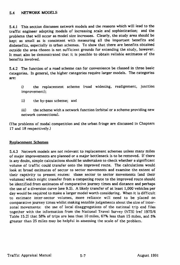
5.4 NETWORK MODELS

5.4.1 This section discusses network models and the reasons which will lead to the traffic engineer adopting models of increasing scale and sophistication; and the problems that will occur as model size increases. Clearly, the study area should be

kept as small as is consistent with measuring all the important benefits and disbenefits, especially in urban schemes. To show that there are benefits obtained

outside the area chosen is not sufficient grounds for extending the study, however. It must also be demonstrated that it is possible to obtain reliable estimates of the benefits involved.

5.4.2 The function of a road scheme can for convenience be classed in three basic categories. In general, the higher categories require larger models. The categories are:

i) the replacement scheme (road widening, realignment, junction

improvement);

ii) the by-pass scheme; and

iii) the scheme with a network function (orbital or a scheme providing new network connections).

(The problems of modal competition and the urban fringe are discussed in Chapters 17 and 18 respectively.)

Renlacement Schemes

5.4.3 Network models of major improvements

are not relevant to replacement schemes unless many miles are planned or a major bottleneck is to be removed. If there

is any doubt, simple calculations should be undertaken to check whether a significant volume of traffic could transfer onto the improved route. The calculations would look at broad estimates of sector to sector movements and examine the extent of their captivity to present routes: those sector to sector movements (and their volumes) which might transfer from a competing route to the improved route should be identified from estimates of comparative journey times and distance and perhaps the use of a diversion curve (see 9.5). A likely transfer of at least 1,000 vehicles per day would be required to make a larger model worth considering. When it is difficult to estimate inter-sector volumes, more reliance will need to be placed on comparative journey times whilst making sensible judgements about the size of inter- zonal movements: the use of local disaggregations of the national trip end files together with the information from the National Travel Survey (NTS) (ref 1975/6 Table 15.2) that 58% of trips are less than 10 miles, 67% less than 15 miles, and 5% greater than 25 miles may be helpful in assessing the scale of the problem.


BY-Pass Schemes

5.4.4 Most by-passes can be handled adequately with models of less than a hundred links and even a major scheme of considerable length does not necessarily demand a major modelling effort. Section 7.3 described how many small by-pass schemes

may be handled. Again, the amount of traffic likely to be diverted from other routes will be the determining factor.

Schemes with a network function

5.4.5 A by-pass scheme will not normally require major network modelling unless it has a network function, usually of a collector-distributor type. Schemes with network functions might typically have either (or all) of : a long length (say greater than 10 kms); many interchanges (say greater than 5); and substantial traffic desires in several directions across the scheme and not solely along its axis. The scheme is likely either to hug an urban area or to be situated between major centres of population.

5.4.6 The scale of the appraisal problem grows broadly in line with the product of the number of zones and links involved. This is not just in the consumption of computer processing time (which is becoming less important as computing costs fall) but also in the requirements of the data base. The number of roadside interview stations required to produce a cordon or screenline also grows rapidly, as do other data requirements, as the study area increases. As models grow in size, the demand for data increases and so, to minimise survey requirements, observed data is translated into sub-models which produce estimates of links speeds, accident rates, and finally trip ends and inter-zonal movements.

5.4.7 Complex models create special problems of model control: as a model expands the traffic engineer must rely more heavily on the model specification; calibration adjustments become more difficult and their effects more subtle. As data in large models will be culled from many sources, special attention needs to be given to the consistency of definitions and the quality of conversion factors.

5.4.8 Whilst trip matrices will have differing demands made of them for accuracy in different sections of the matrix (usually the corridor and local area of scheme require greater accuracy), the number of cells in a large matrix which are relatively unimportant is very much larger; these latter cells can often contain estimates of low accuracy without affecting the model’s suitability for the scheme under appraisal.


‘L

54.9 This section has discussed the relationship between network models of increasing size and the different types of schemes which may require appraisal. The principles discussed apply equally to rural or urban roads, and it is not the physical size of the scheme but its implications for travel behaviour which determine the method of appraisal. In summary, the traffic engineer should always be reluctant to increase the scale and complexity of a network model unless he is satisfied that the extra costs involved (and probably the extra data collection and the lengthening of the study period as well) are justified by the problem in hand.

5.4.10 In choosing the appraisal method, the traffic engineer should always start with the simplest approach that could be hoped to give the required information and extend this only when it becomes clear that the modelling of important aspects of the scheme is inadequate. Every effort should be made to complete the development of the method before survey work has commenced, however, as it is inefficient to design and implement traffic surveys in piecemeal fashion.


5.5 DYNAMIC TRAFFIC MODELS

L

L

L

5.5.1 Since the mid 197Os, a number of dynamic traffic models have been developed. Usually based on a hybrid of analytic and simulation techniques, these models provide a means of synthesising vehicle (or pedestrian) movements around road and junction layouts. The effect of changes to the road network on traffic flows and delays can thus be observed and reported. Two types of model are currently employed in the UK.

5.5.2 Traffic assignment models have been developed to provide more accurate descriptions of traffic movements in urban areas, where journey times can be greatly increased in congested conditions and the effects of traffic management schemes must be considered. These models have as inputs the desired trip matrix (perhaps as a function of time) and the cost/flow characteristics of the road network. Traffic is then assigned to the network by a variety of methods, and flows, delays and journey costs are monitored. There are a number of models available in the UK at present, depending on the information required for the appraisal:

i) the option to vary demand over time is provided by CONTRAM (ref 21, SATURN, HINET, TRIPS, for the assessment of peak traffic.

ii) the detailed modelling of junctions and the coordination of traffic signals, which may be important in urban studies, are features of SATURN, and to a lesser extend of JAM and HINET; TRIPS and CONTRAM provide an indirect form of signal coordination.

iii) in addition to journey time information, SATURN and CONTRAM model fuel consumption.

iv) facilities for comprehensive transport planning are provided by TRIPS and ASSIGN, as would be required in appraisals where trip distribution and mode choice were important.

5.5.3 Simulation models for more detailed modelling of traffic management schemes have been developed, for example TRAFFICQ (ref 3). This program provides information in terms of journey times, costs and delays for individual vehicles on selected routeings through the networks, but a wide range of traffic management options can be evaluated, including priority and signal controlled junctions, roundabouts and pedestrian crossings. It should be noted, however, that TRAFFICQ is not an assignment programme and the routs taken by trips through the network

must be specified.

5.5.4 The use of these models in trunk road appraisal is also discussed in Chapter 14. They are used primarily for the analysis and design of traffic management schemes and the operational analysis of congested networks. They will be most commonly applied to urban problems, but it should again be stressed that an urban setting does not in itself justify their use. It must still be established that the extra costs involved are offset by the value of the information obtained.


5.5.5 The problems remaining are those associated with variable trip matrices. The origins of the extra traffic may be generated trips, trips attracted from other origins / destinations, traffic attracted from parts of the network external to the scheme, trips made by other modes, or trips made at a different time of day. If possible, changes in the trip matrix should be estimated once and for all and re-assigned to the network, but in large urban schemes this process may need to be iterated until a satisfactory solution is found.

5.5.6 A fundamental difficulty with variable trip matrices arises in the economic assessment of the scheme, when the benefits accruing to trips which were not being made before the improvement must be estimated. The information required for this purpose can be expressed in terms of the elasticity of demand (for trips of a particular type) with respect to the generalised cost of travel; so as travel times in the peak increase, a proportion of travellers will re-time their journeys to travel at less congested times, and the objective of research here is to quantify this effect. A number of research studies which bear on these problems are going on at present.


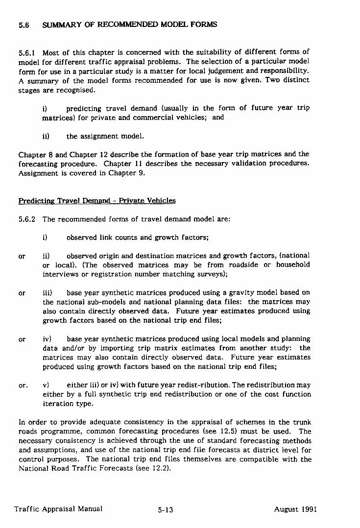
5.6 SUMMARY OF RECOMMENDED MODEL FORMS

5.6.1 Most of this chapter is concerned with the suitability of different forms of model for different traffic appraisal problems. The selection of a particular model form for use in a particular study is a matter for local judgement and responsibility. A summary of the model forms recommended for use is now given. Two distinct stages are recognised.

i) predicting travel demand (usually in the form of future year trip matrices) for private and commercial vehicles; and

ii) the assignment model.

Chapter 8 and Chapter 12 describe the formation of base year trip matrices and the forecasting procedure. Chapter 11 describes the necessary validation procedures. Assignment is covered in Chapter 9.

Predicting Travel Demand - Private Vehicles

5.6.2 The recommended forms of travel demand model are:

or

or

or

or.

i) observed link counts and growth factors;

ii) observed origin and destination matrices and growth factors, (national or local). (The observed matrices may be from roadside or household interviews or registration number matching surveys);

iii) base year synthetic matrices produced using a gravity model based on the national sub-models and national planning data files: the matrices may also contain directly observed data. Future year estimates produced using growth factors based on the national trip end files;

iv) base year synthetic matrices produced using local models and planning data and/or by importing trip matrix estimates from another study: the matrices may also contain directly observed data. Future year estimates produced using growth factors based on the national trip end files;

v) either iii) or iv) with future year redist-ribution. The redistribution may either by a full synthetic trip end redistribution or one of the cost function iteration type.

In order to provide adequate consistency in the appraisal of schemes in the trunk roads programme, common forecasting procedures (see 12.5) must be used. The necessary consistency is achieved through the use of standard forecasting methods and assumptions, and use of the national trip end file forecasts at district level for control purposes. The national trip end files themselves are compatible with the National Road Traffic Forecasts (see 12.2).


Predicting Travel Demand - Commercial Vehicles

5.6.3 Commercial vehicle estimates may be required in traffic studies for a number of purposes. Estimates are required for COBA; for geometric design; for the calculation of standard axles in pavement design; for environmental appraisal

(particularly in the calculation of road traffic noise); and in the detailing of designs and ancillary traffic management.

5.6.4 There is no doubt that these vehicles cause more public concern than private vehicles and the estimation of commercial vehicle volumes is a most important element of traffic appraisal. In particular, the Minister has recently received a report by Sir Arthur Armitage (ref 4) which is at present being studied. When the Department’s current requirements for quantitative estimates of commercial vehicle flows are reviewed individually it is found that, whilst estimates of commercial vehicle volumes are vital, the quality of the forecasts from current appraisal procedures will be sufficiently sensitive for most uses. For example, the difference between providing a pavement thickness to cope with 150 million standard axles (msa) rather than 30 msa adds about 5% to total works cost; similarly, the amount of noise from road traffic is not sensitive to small changes in the percentage of heavy vehicles (a doubling of the percentage of commercial vehicles from 10% to 20% at a typical traffic speed might add 14 dB(A)).

5.6.5 The estimation of commercial vehicle trip movements will rely heavily on direct estimates from roadside interviews with the possibility of infilling by use of the partial matrix method (see 8.3). SACTRA acknowledged the RHTM commercial vehicle matrices to be the best source of national information available but these should be validated locally before use in a particular scheme appraisal (see 8.4).

5.6.6 Very heavy vehicles (those greater than 25 tonnes gross vehicle weight) are predicted to grow faster than commercial vehicles of lower weight: these vehicles also have a very much longer than average length of haul (see Figure 5.1). But unless special attention is paid to sampling or a special modelling approach adopted, normal interviewing is unlikely to produce an adequate sample of these vehicles to allow separate identification of their movements. However estimation of the proportion of these vehicles by different weights sufficient for some purposes can be obtained by road type after assignment (see 12.3).

5.6.7 The recommended forecasting procedure for commercial vehicles, and that used in COBA, is based on national growth factors which are now applied by 3 weight classes. The range of the NRTF for this sub-group of vehicles, when taken together with the uses of commercial vehicle forecasts, is sufficiently wide for local planning purposes (see 12.3). Local re-distribution of commercial vehicle trip matrices may however be undertaken within the forecasting procedures (see 12.3), providing that the growth predicted in the commercial vehicle kilometreage of the study area is constrained to that of the predicted NRTF growth (see 12.3).


5.6.8 A report on commercial vehicle forecasting undertaken under the purview of the RHTM Project (ref 5) reviewed trends from the continuing Survey of Roads Goods Transport (see 4.7) and discussed the problems inherent in disaggregate commercial vehicle forecasting. The Department is considering whether it is desirable to develop improved commercial vehicle forecasting methods for scheme appraisal.

Methods of Assignment

5.6.9 The allocation of a trip matrix to a network (assignment) may be carried out by a number of methods which are described in Chapter 9. The simple assignment methods are:

i) manual assignment (including multi-routeing by use of diversion CUIWS);

or ii) all-or-nothing assignment.

More complex methods can be classified according to the particular facilities which they contain (they are not mutually exclusive). For studies of networks with closely competing routes in the corridor of interest, it is necessary to share traffic between those routes to some extent. In such cases a multi-routeing facility may be necessary. For problems which involve congested networks, which are only found in larger urban areas, capacity restraint or where junctions significantly effect one another, dynamic traffic models are available (see 13.4).


FIG. 5.1

TRIP LENGTH & LENGTH OF HAUL BY VEHICLE SIZE 1973-1978

L1 - 60,

-. c

-28 - 32 tonnes

/-1 over 32 tonnes

40

1 --\ 20

_- *. urldc~ 5zc _ _ - - - - .*.______-----

tonnes

I__ ,.~~ , T 1 T ---1 1970 1974 1975 1976 1977 1978

TRIP LENGTH BY VEHICLE SIZE LENGTH OF HAUL BY VEHICLE SIZE

14c

120

40

20

b

1 1

1

I ”

n over 32 tonnes

~~~-~~~

_--

___a-- --\

lnder S’$J- . .

,

. . ,’

tonnes \------’

-T--~- T ANT 7.- --1

1973 1974 1975 1976 1977 1978

_ _

5.7 SELECTION OF TIME PERIOD FOR APPRAISAL

L 5.7.1 There are two levels of traffic analysis. Firstly, for appraising the overall

worth of a scheme, an estimate is needed of the total traffic that the scheme will carry during its economic life, together with an estimate of the frequency and duration of different loadings. Secondly, and as an extension to the first, there is often a need for a more detailed analysis in the immediate locality of a scheme to ensure that the local impact of alternatives is fully appreciated: this is known as operational appraisal (see Chapter 13).

5.7.2 For most appraisals, both economic and operational, the assigned daily link flows can be factored to give estimates of any desired traffic loading (see 6.10). This is the procedure COBA uses.

L

5.7.3 In some cases, usually in congested networks, the more detailed operational appraisal may demand that behaviour under congestion be specifically examined. There may be concern that traffic will come to a halt (for example, gyratory systems may “lock” because of inadequate queueing space) or that the local road network cannot disperse traffic terminating from a new route. In virtually all cases a factored daily trip matrix should provide an adequate representative peak loading under which to examine a scheme or provide an hourly flow rate suitable to produce an appropriate set of routes for capacity restrained assignment (see 9.5). Directionality can also be obtained by factoring.

5.7.4 In extremely rare cases in trunk road appraisal, a direct peak period model (that is, based on directly formed matrices from peak period interviews) may be judged to be preferable: such models are usually the preserve of short term urban forecasters or studies where an exceptional interview base can be obtained in the peak period. Before a decision to use such a model is made, the following questions should be considered:

i) What is the purpose of the model ? What decisions are required of it? Would decisions based on a peak hour model be different or better than those based on a factored daily model?

ii) The accuracy of the trip matrix elements, whether the matrices are observed or synthetic, is related to the number of interviews on which the estimates are based. How many interviews will be required, compressed into the peak period, to make the forecasts significantly different from a forecast factored daily matrix?

iii) What is the definition of the peak period to be modelled? Why is this definition better than a factored daily model ? If directionality is important, how many peak periods should be considered?


5.7.5 In summary, it is the Department’s view that daily trip matrices (based on 12 hour weekday interviewing) are usually preferable for trunk road appraisal purposes (see 8.1). The few appraisals requiring peak period matrices can obtain these by factoring the daily matrix (see 6.10); these matrices will often be cordon matrices and will be applied to congested areas of network probably using dynamic traffic engineering methods (see 13.4). Peak period routeing effects can be embraced in capacity restrained assignment (see 9.5).



1. Robertson D I: “TRANSYT - a traffic network study tool”, LR253, TRRL 1969.

2. Leonard D R, Tough J B and Baguely P C: “CONTRAM - a traffic assignment model for predicting flows and queues during peak periods”, LR841, TRRL 1978.

3. Logie D M W: “TRAFFICQ - A Comprehensive Model for Traffic Management Schemes”, Traffic Engineering and Control, November 1979.

4. “Report of the inquiry into Lorries, People and the Environment”, HMSO, December 1980.

5. Jam&on Mackay and Partners: “Commercial Vehicle Forecasting”, RHTM project, Department of Transport, 1980.


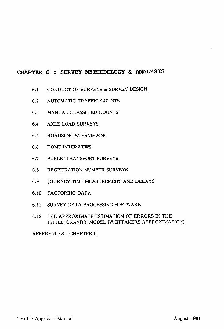
6.1

6.2

6.3

6.4

6.5

6.6

6.7

6.8

6.9

6.10

6.11

6.12

6 : SURVEY METHODOLOGY & ANALYSIS

CONDUCT OF SURVEYS & SURVEY DESIGN

AUTOMATIC TRAFFIC COUNTS

MANUAL CLASSIFIED COUNTS

AXLE LOAD SURVEYS

ROADSIDE INTERVIEWING

HOME INTERVIEWS

PUBLIC TRANSPORT SURVEYS

REGISTRATION NUMBER SURVEYS

JOURNEY TIME MEASUREMENT AND DELAYS

FACTORING DATA

SURVEY DATA PROCESSING SOFTWARE

THE APPROXIMATE ESTIMATION OF ERRORS IN THE FITTED GRAVITY MODEL (WHITTAKERS APPROXIMATION)



CHAPTER 6 : SURVE~YMETHODOL~GY &ANALYSIS

6.1 CONDUCT OF SURVEYS & SURVEY DESIGN

Necessitv of Surveys (General)

6.1 .l DTp Ministers are concerned to ensure that survey work is directly relevant to policy needs (immediate & long-term), provides value for money, and minimises the burden on respondents. This means that no traffic survey should be planned

unless it is clear why the information is needed, that there are no alternative sources for this information, and that the cost, timing and location of the survey are reasonable. A review of current data available, and planned data collection, should be carried out both nationally (see Chapter 4 for a review of available data) and locally, to ensure that the requirement for data cannot be met from an existing source.

6.12 Survey approval must be obtained from EEA division before fieldwork can start. Discussions with EEA Division should take place at an early stage so that the data base for appraisal and (where necessary) a programme of data collection can be agreed.

6.1.3 If a survey is essential, care should be taken in deciding its form. A distinction should be made between those surveys which involve disturbing the public, particularly interview surveys, and those which do not, eg traffic counts. When the data needed can be collected economically in different ways, the least intrusive should be chosen. For example, registration number matching techniques may sometimes be suitable for small origin and destination surveys and these are, on balance, less intrusive than roadside interviews.

6.1.4 An ‘interview survey’ is an enquiry for which the purpose (or part purpose) is to compile statistics for administrative or research use whether by a full census or a sample survey, regular or ad hoc, conducted by post, telephone, or face to face interview. The respondents may be individuals, households, businesses, local authorities, or other bodies outside central government. Roadside and household interviews both come within this definition.

6.1.5 The handling of survey data must conform to data protection standards. Results must be presented anonymously, and should not otherwise be divulged without appropriate authority. A confidentiality assurance to this effect may be given as part of the data collection procedure.

Control of Roadside Interview Surveys

6.1.6 EEA Division has delegated authority to process and clear all roadside interview surveys pertaining to the roads programme. They will inform project managers when a survey has been approved and notified to the Minister and the

Survey Control Unit (STDS).


Other surveys, eg surveys of households, businesses or local authorities, are dealt with by the Survey Control Unit.

6.1.7 The procedures for controlling roadside interview surveys carried out by the Department are outlined in a Heads of Division circular, which is revised from time to time. In particular, note that Ministerial approval will be necessary to start or continue surveys during a General Election campaign. Planning for roadside

interviews is unlikely to be disrupted by local government elections, unless the survey is somehow associated with a controversial local issue. EEA division should be informed if this is the case.

6.1.8 Detailed arrangements for roadside interview surveys are as follows. At least 4 weeks before fieldwork is due to start, the following revised forms and attachments must be forwarded to EEA Division:

Technical Vetting Form (SCU) Customer Division Form (CD) Traffic Survey checklist draft Press notice plan showing location of interview sites.

The SCU form, CD form & checklist should be copied to STD3.

6.1.9 The proposed new roadside interview survey must be reported to EEA Division in time for discussions to take place on the necessity for and extent of the survey, and the locations where survey sites are thought necessary. Approval may be delayed if the information sent to EEA is incomplete. In particular, project managers are asked to ensure that the cost of the survey to the Department is correctly shown. It is important that financial provision for survey work has been made.

6.1.10 Note that roadside interview surveys carried out by Local Authorities for their own purposes are not within the scope of the system outlined above. However the Local Authority does need Department of Transport permission to carry out surveys on a Trunk Road. The granting of this permission is delegated from the Secretary of State to the Regional Office. The Advice Note on Roadside Interviews (ref 1 )

contains detailed advice on the layout of the interview sites which should be noted by the Regional Office when considering requests from Local Authorities


This completed form must be returned to: SURVEY CONTROL UNIT (SCU)

STD3, B6+4 ROMNEY HOUS&, 43MARsRAM STREfi LONDON,SWlP 3PY 07 l-276 8269

via the customer division as follows: standard traffic, follow-up, repeat, pilot household surveys and household surveys which are part of an agreed EC initiabve, an approved research project, or COI campaign b at least 2 weeks before start of fieldwork

other surveys b at least 4 weeks before start of fieldwork

IA] SPONSOFUNG DIVISION TO COMPLETE

Name of contact

Division

Address

Date forwarded to customer divtsion

Customer diviston

Customer division contact

Teiephone Latest date for submtssion by customer dinston to SCIJ __

Al TITLE OF SURVEY

A2 PURPOSE OF SURVEY

1 Type of survey: ad hoc/vohtnt&/statutoty - --

2 Indicate which (if any) of the followmg applies:

The survey repeats earlier work 0

The survey has been piloted 0

>e survey is a pilot study 0

The survey IS a fo~ow-up study 0

3 Detatls of any earlier relevant sweys

Expected response rate

Tie burden on each respondent _

Dates and durahon of fieldwork

Is part or all of survey to be carried out by a ‘body outsIde Ihc depanment

YESO -nameofbody

-fee(mc. VAT) L _

NOI

.,.

10 Estimated internal cost to the department of carrying ou! the

survey (including staff and compuang costs) C _-_ 4 Respondents: BusmessIHouseholds or

indtviduals/Local Authonhes

5 Number of respondents

11 Estimated date (month/year) of publication of results _

L, lB] (SPONSORING DMS

For appratsal of scheme in road! programme

Part of approved research programme

Already approved. in pnnclple. by mmlsters (includmg agreed EC mitlattve)

Fol!ow-up to an earher approved survey or a repeat survey

L Xher suney

i

COMPLETE ONE SECTION ONLY V

ls appraisal expected mthm next 12 months?

ls completed checklist attached?

=I

NO0

=O NO0

SAG reference number Attach copy of relevant Project Record

Date of approval Attach copy of relevant references. mth Muuster’s name

Date of prevtous survey

Date of mmlstenal approval Attach copy of relevant references

Traffic Appraisal Manual 6-3

Pass form to EtiA (copled to SCU) for completion of C3 and c4 -

Pass form to customer Qvlston for completion of Cl, C3 and c4

Pass form to customer dlvlsion for completion of Cl. C3 and c4

Pass form to customer dlvls:on for complehon of C3 and C4

Pass form to customer dmsron Ior compbnon of sectton C _.. _

August 1991

[C] POLICY SUPPORT (CUSTOMER DMSION TO COMPLETE)

COMPLETE Cl OR C2, AND C3 AND C4

Ci The survey has already recewed mmistenal approval. or is part of an approved research programme or an agreed EC mtmv4

d a. Does the survey/research programme sull have customer YESO

drwslon support? NO c]

b. Are the content, tlmmg. and location of the survey acceptable? YESO

NO 0

C2 The survey has not yet received prior authonsaoon

a. Poky )ustAcanon:

_- .-

b. Does the informanon to be collected justify the estimated costs? y=czl 4

NO 0

c. Are the content. nming. and location of the survey reasonable? =I

NO0

C3 Comment (if any)

i --

C4 Name (Grade 5 or above) Date --

Signature

Customer divisron contact Divtslon ---

Address and telephone

Date forwarded to SCU

[D] TECHNICAL ASSESSMENT (FOR SCU USE. see Note)

Dl Recognmon provided by CSO (SCUI Not requued I In pnnclple / -’ Full

D2 Recogmaon proovlded by DTp WV Not requtred I In pnnciple I Full

[El MINISTERIAL APPROVAL (FOR SCU USE)

El Mimstenal Approval requued

E2 Mlmstenal Approval obtamed

Date

File Ref.

Note: Dl applies to surveys of busmesses or local authonties

* D2 applies to surveys of households or mdividuak

Traffic Appraisal Manual 6-4 Au/just 1991

SURVEY CONTROL: REGIONAL OPERATING UNITS - TRAFFIC SURVEYS CHECKLIST

1.

u

2.

Title of Survey

Date of Survey

3.

4.

Survey Control Form completed

II II 11 sent to EEA Division

5. II II II copied to SCU Romney House

6. Customer Division Form (Parts A & B) completed

7. II II II sent to EEA Division

b 8. II II copied to SCU Romney House

9.

10.

11.

L- 12.

13.

Press Notice - prepared/drafted

- sent

Letter to MPs - prepared/drafted

- sent

Police consulted

Police attendance at site arranged

Highway authorities consulted

---

Please d Box

When completed, this form - together with items 3, 6, 9, and 10 above - should be forwarded to EEA Division with copies to the Survey Control Unit. Addresses are as follows:

EEA Division Room S4/19

Survey Control Unit Room B644

2 Marsham Street Romney House LONDON 43 Marsham Street SWlP 3EB LONDON SWlP 3PY


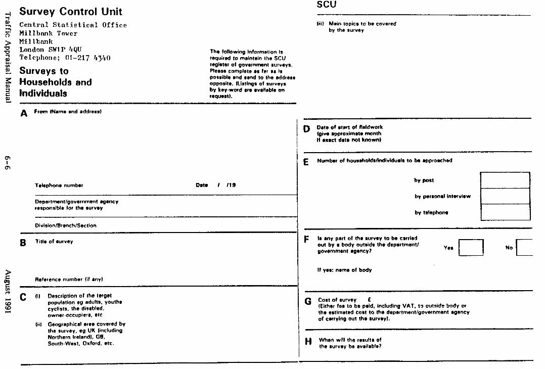
Survey Control Unit Central Statistical Office Millhnnk Tower Milllxnlc London SHlP 4QU Telephone; 01-217 4340

surveys to

Households and Individuals

lho foltowing fnformstion Is required lo maintain the SCU register of government rurveys. Pleese complete as far as fs possible and send to the eddrssr opposite. (Listing8 of l urvevs bv key-word 8re l veil&fe on requert).

A From IName rnd rddresrt

Tekqhone numbef tme I 119

Department/government egency responsible for the rurvry

DivisionlBranchlSection

B Tit10 of survey

Reference number fif rnyl

Description of the target populetion eg sdults. youths cyclists. the disabled. owner-occupiers, 0tC

Geogrsphicsl erect covered by the survey, sg UK (including Northern Ireland), GE. South-West. Onford, etc.

scu

fiii) Main topics to be covered by the survey

D Date of start of ftefdwork fgive l pproxirnato month If exact date not known)

E Number of houreftofds/tndividuaIr to be agproeched

b mt

by personel interview

by telephone

F Is my part of thr rurvev to be carried out by l body outside the depmrtmentl government egencv? Yes I] No r

If yes: nrme of body

G Cost of survey E (Either fee to be peid, including VAT. to outside body or the estimated cost to the department/government agency of currying out the rurveyl.

H When will the result@ of the survey be rvrilrble?

Planninn A Survey

6.1.11 The following subsections summarise the technical and organisational decisions to be made in the course of planning a successful interview survey.

Obiectives and Resources

6.1.12 The survey objectives must be precisely laid down. It is not enough to say that the survey is intended to find out about ‘travel habits’. The initial statement should say why the survey is being done, exactly what questions will be asked and the kinds of results expected.

6.1.13 Writing such a statement will clarify requirements in the mind of the person responsible, and should lead to a more efficient survey. Once objectives are settled, the plan is to achieve them to required accuracy and within the given resources.

6.1.14 When the objectives of the survey are clear, the review of current data available should take place. If available data sources are inadequate then planning of a new survey can proceed.

Coverage

6.1.15 The population (the aggregation of persons or objects under investigation) to be studied must be defined - the geographical area, the road, the households - all need to be spelt out. If people are to be interviewed, the method of selecting the interviewees has to be determined to ensure a statistically valid sample.

6.1.16 The person responsible will be faced with a list of questions such as: What type of sample is to be used ? What is the appropriate sampling unit (LA District or constituency; ward or polling district; household, family or individual; car occupants or driver only etc)? What sampling frame (a list of some sort of the population being studies) is available in the case of household interviews? What are the deficiencies of any such sampling frame or list ? How big a sample is required for the desired accuracy? How big a sample is feasible within the constraints of the available resources?

Method of data collection

6.1.17 The choice of method used for collecting the data depends on the subject, who the respondents are and the scale of the survey. For household surveys, postal questionnaires with or without a follow-up personal interview, or purely personal interviews can be used. For roadside surveys a short interview is normally conducted.


Ouestionnaires

6.1.18 Many types of surveys use questionnaires of one sort or another. This is perhaps the most neglected survey task. It is vital that decisions in areas such as the scope of the questionnaire, the definitions and instructions, and the wording and order of the questions are taken only after proper consideration. Before the questionnaire is finalised the Survey Control Unit (see 6.1.2 above) must be consulted via the EEA Statistician and STD Division.

Timinz of surveys and cost

6.1.19 Factors to be taken into account to decide when surveys should be carried out include the time(s) of the year - are holiday periods etc to be avoided ? - the day(s) of the week, the time(s) of the day. Also, if a sampling frame such as the electoral register, which is updated annually, is being used it might be worth waiting until just after it has been updated.

6.1.20 Once the date of the survey is fixed a timetable can be drawn up for each stage and a cost estimate made. Standing instructions in a Heads of Divisions Notice (THOD 3/84) state that MPs should be alerted when the Department proposes to carry out a field experiment to conduct a survey which is likely to impinge on local issues in their constituency. Draft letters to MPs should be submitted by the Head of Division to the Private Office of the relevant Minister. If a press notice with a compliments slip from the Minister will suffice, the Head of Division should make the necessary arrangements with the Private Office.

Fieldwork

6.1.21 The quality of interviewing is of obvious importance in both household and roadside interviews. Training of interviewers needs to be taken into account, as does the extent and method of field supervision. Checks on the integrity and efficiency of interviewers should not be neglected.

6.1.22 Respondents should always be told, by letter or handout, how they were chosen, whether co-operation is voluntary, the purpose of the survey, who it is for, what confidentiality arrangements apply, and where to make enquiries. Copies of the letter or handout should be sent to STD Division, via the EEA Statistician.

Processing and Analvsis

6.1.23 The processing and analysis of survey data is a very large area of work. When questionnaires or data sheets come into an office, or earlier if possible, they must be scrutinised for errors, omissions and ambiguous classifications, before they are ready for coding and tabulating. In order to facilitate this an editing scheme should be devised, together with code lists and some ideas for tabulations and analysis plans.


Samnlinn factors

6.1.24 The method of analysis to be used, ie whether manual or computer analysis, should be decided. If the latter, the programs will either have to be selected or written (if a suitable program is not available). If weighting or grossing up is to be carried out the method and means of doing this should be decided. A survey analysis package to link in with ROADWAY is under development.

Pilot Survevs

6.1.25 From the brief review of the considerations mentioned already it will be clear that a number of things need to be known before an efficient survey can be planned. Where historical data or prior experience is not available the best way of acquiring this knowledge is by undertaking a small survey, known as a pilot survey. A pilot survey will provide guidance on:

i) the adequacy of the sampling frame;

ii) the variability of the population being studied;

iii) the non-response rate to be expected;

iv) the suitability of the method of data collection;

v) the adequacy of the questionnaire;

vi) the efficiency of the instructions and general briefing of interviewers;

vii) the codes chosen for pre-coded questions;

viii) the probable cost and duration of the main survey;

ix) the efficiency of the organisation.

6.1.26 These are dealt with separately in the sections covering the different types of surveys.

Confidence limits

6.1.27 When an estimate of traffic flow has been made, it is desirable to know not only the estimated value but also how reliable this estimate is. A convenient way of expressing the precision is to state limits which, with a given probability (usually 95%) include the true value. It is then possible to state, for example, that the true value is unlikely to exceed some upper limit, or to be less than a lower limit, or to lie outside a pair of limits. This information may be more important than the estimate itself.


These limits are known as “confidence limits”, ie they are limits within which it can be stated, with a given degree of confidence, that the true value lies.

6.128 The adoption of a particular confidence interval implies a decision concerning the accuracy required of the information presented: for example, a 95% confidence interval accepts the chance that the true value will lie outside the given limits only 5 times in 100 occurrences. The greater the accuracy demanded of the data the wider the confidence interval will be, as follows:-

accepting 32 occurrences in 100 outside the limits by chance gives limits f 1 standard deviation

accepting 5 occurrences in 100 outside the limits by chance gives limits of f 2 standard deviations

accepting 1 occurrence in 100 outside the limits by chance gives limits of L 2.58 standard deviations


6.2 AUTOMATIC TRAFFIC COUNTS

L

L

6.21 Automatic traffic counting (ATC) is an operation requiring a substantial investment in instruments, ancillary equipment, transport, data handling systems and staff time. The volume of data that can be collected is considerable, but the effort expended can prove fruitless and the data obtained worthless if any one of the many constituent processes involved in collecting and processing the data is deficient. At the same time a balance has to be struck between the considerable additional effort that could be expended and the limited additional accuracy or detail of the data then obtained.

6.2.2 The purpose of ATC is to obtain a best estimate of the volume of traffic on a section of road. The manual produced by EEA division (A Manual of Practice on Automatic Traffic Counting - ref 2) provides guidance on the conduct of ATC whether it is being carried out at a site over a short period, regularly, or continuously, and which when followed will meet the objective in a way which is consistent with the resources and effort put into the work.

6.2.3 Little definitive work has been published concerning the accuracy of traffic counts by automatic traffic counters. Experience suggests that the errors are machine and (particularly) installation dependent, TRRL Supplementary Report 5 14 (ref 3) contains some useful results on the efficiency and accuracy of annual estimates from short period counts. For longer term counts, the frequency and diligence of the station monitoring and servicing will be crucial.

6.2.4 Intrinsically, inductance loop detection should be more reliable than pneumatic tube detection. However, to obtain high quality results with loop detectors on multi- lane sites it is essential that the loop installation is of the highest quality and generally implies the use of a frequency meter. The major drawback with pneumatic tube detection, now that high quality electronic air switches are available, is that they count the number of axles (or pairs of axles) rather than the number of vehicles which is the required quantity. A factor must then be applied to convert to the number of vehicles that went by, an additional source of error over and above the “mechanical” error of the counting apparatus itself. The use of a single loop detector on a multi-lane road is bound to result in undercounting. TRRL Supplementary Report 473 (ref 4) describes a theoretical method of allowing for this undercounting.

6.2.5 Using the limited information available, the current best “working” estimate of the accuracy of measurement of the number of vehicles that passed an automatic traffic counter is that the 95% confidence interval of a count of longer than 12 hours duration is of the order of f 5% of the total count (Before and After studies: Stage II Report - ref 5). This assumes that the counter was installed and maintained to the standards laid down in “A Manual of Practice on Automatic Traffic Counting” (ref 2). Recent work by the GLC supports this assertion (ref 6). While counting for longer periods will yield more data, and will help to reduce the impact of human blunders and mechanical errors, it is unlikely that confidence intervals can be much reduced. This is because the data are correlated, the same counting equipment being used on the same site on contiguous days, and independent data are required to substantially increase accuracy.


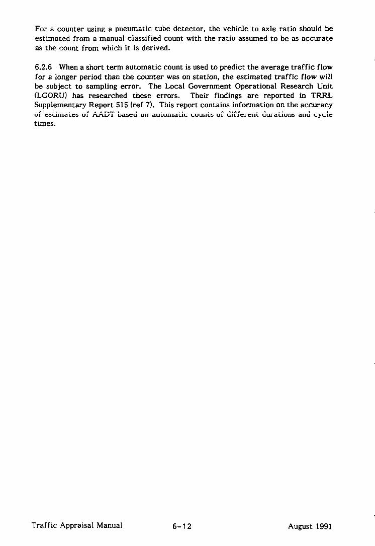
For a counter using a pneumatic tube detector, the vehicle to axle ratio should be estimated from a manual classified count with the ratio assumed to be as accurate as the count from which it is derived.

6.2.6 When a short term automatic count is used to predict the average traffic flow for a longer period than the counter was on station, the estimated traffic flow will be subject to sampling error. The Local Government Operational Research Unit (LGORU) has researched these errors. Their findings are reported in TRRL Supplementary Report 515 (ref 7). This report contains information on the accuracy of estimates of AADT based on automatic counts of different durations and cycle times.


6.3 MANUAL CLASSIFIED COUNTS

s

L

General

6.3.1 There are no general guidance rules for carrying out Manual Classified Counts. The number of enumerators required will depend on the flow on the road under consideration. As a rough guide one enumerator could probably handle about 500-600 vehicles per hour.

6.3.2 If each enumerator is assigned particular types of vehicles this will help to spread the load.

6.3.3 Detailed advice on counting can be obtained from STC Division in the Department.

Instructions to Enumerators

6.3.4 The form currently used by the Department and Traffic Census Division is shown at figure 6.2. This is slightly different to that used in the RHTM project. This is found to work well in practice. A fresh sheet should be used for each hour or half hour. As each vehicle is counted the next number in the appropriate box should be cancelled. At the end of the hour or half hour or other short period the last cancelled number should be entered in the appropriate total box. A note should be kept of any events which seriously affect flow in any hour, eg weather, road works (including diversion from another road), accidents and convoys of many vehicles. These can be coded at the bottom of the sheet. For high volumes, the use of hand tallies can be valuable.

Vehicle Catepories

6.3.5 The types of vehicles to be distinguished are shown on each form with a silhouette showing one example of the various vehicle types covered in each section. The following explains what the categories cover:

i) Two wheeled motor vehicles include motor cycle combinations.

ii) Cars and Taxis include estate cars and all light vans with side windows to the rear of the driver’s seat (eg minibuses, “Microbuses” and “Dormobiles”). They also include three wheeled cars, “bubble cars”. and motor invalid carriages.

iii) Buses & Coaches include works buses, but not minibuses or

“Microbuses”.

Traffic Appraisal Manual 6-l 3 August 1991

AAS AND TAXlS

2 3 4 5 6 8 9 10 11 12 13 14 15 16 17 18 19 20 21 22 2: 24 25 26 27 28 2 30 31 32 33 34 35 36 37 38 3Q 40 41 42 43 Lo 45 46 47 48 49 50 51 52 53 54 55 56 57 58 59 60 61 62 63 64 65 66

67 68 69 70 71 72 73 74 75 76 77 78 79 90 81 02 83 84 85 86 97 88 89 90 91 92 93 94 95 % 97 96 %1001011021031M1051%107108109110111112113114115116117118119120 121 122123124 125126127 128 129 130131132133134135136137 138 139140141 142 143 144 145 146 147 148 149 l!Y_l 111 152 153 154 155 156 157 158 159 160161 162 163164 165 1% 167 168 169 170171 172 173 174 175176 177 178 179180181 182183184 185 188187188189190191 192193194 195 196 197198 1992W2Ot 2022032042OS 2062012082OQ210211 2122132142152162172r82r9220221222223~42252262272?B ~230231232233234235238237i382392402412422432U24S2~247208249250291252253254255 ~2572~2592~26126226326*2652%2672%2692702712722732742?5276277278279280281282 1831Bot8S3862872~8289f90t41t92t93~~S298297298199~30130230330rl305306307308309 31031131231331431531631731831Q32032132232332432532632732832933C331332333334335336 U735835Q3oO341~23a3jM3a6306407Y83493507513523533~355356357356359360361362353 ~365366367368369370371372373374375376377378379JBO381382383384185386U17388~Q3QO 391 3923933943953%397398~*00rO1*02L03oOa~*08U)?U)80094104114124134144154t6417 4184194204214224234244X4264274284X4304314324534JO~5436437438439M0rO1042*O3~ US**6M7U8UQ4604614524534544554%4574%459~061*62063*6r)~5166o87*68069470471 4724734744?4476477478479400~l*82183~~5486*874884894904914924Q3494495496497498 ~S~5015M5035M505506507508509510511512513514515516517518519520521522523524525 526527529529530531 532533534535536537 538539S40541542 5d354454564654754654955055l 552 553 554555556657 5% 559560561 562 5635645655% 567 568569670571572573574S75576 57-l 570579 590 581 582 583 584585 586 587 588 589 590591 592S93 594 595 596 597 598 5% 600601 602 603604605606 807606609610611612613614615616617618619620621622623624625626627626629630631632633 gja6366366376386396+0~lr2br13~6*5~607~~96x,651652653654655656657658659660

76 77 78 79'80 81 8? 83 64 85 86 88 89 90 91 92 93 94 9S 96 97 98 99100101 102 103 104 105 106107 1oB 106 110111112113 1 15116117 118119 120121 122123 124125 126 127 128129 130 131 132 133 134 135 136 137 138 139140 1 42143 lUl46 146147 148 149 150 151 152153 1541551% 157 158 159 160 161 162 163164165166167 1 69170171 172173174175176 (77178 179 180181182183

HEAVY GOODS V' HICLESWITW 3 AXLES

WEAVYOOODSVE~ICLESWITH AAXLESIAATlCUUlEDORWlTn TRAILER)

COMMENTS lif l vl Flooding-A Fog-C Aahntaawootw-E Wetred-G

Figure 6.2 horr-8 Rod Watu- D Dlvwsmn-F


71

Tl,

12 23 24 25

26 27 29 2Q 30

7

59 60 61 62

pq-j-q---

4

4

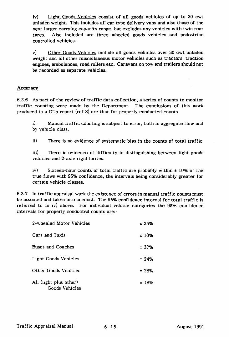
iv) Light Goods Vehicles consist of all goods vehicles of up to 30 cwt unladen weight. This includes all car type delivery vans and also those of the next larger carrying capacity range, but excludes any vehicles with twin rear tyres. Also included are three wheeled goods vehicles and pedestrian controlled vehicles.

v) Other Goods Vehicles include all goods vehicles over 30 cwt unladen weight and all other miscellaneous motor vehicles such as tractors, traction engines, ambulances, road rollers etc. Caravans on tow and trailers should not be recorded as separate vehicles.

Accuracv

6.3.6 As part of the review of traffic data collection, a series of counts to monitor traffic counting were made by the Department. The conclusions of this work produced in a DTp report (ref 8) are that for properly conducted counts

i) Manual traffic counting is subject to error, both in aggregate flow and by vehicle class.

ii) There is no evidence of systematic bias in the counts of total traffic

iii) There is evidence of difficulty in distinguishing between light goods vehicles and Z-axle rigid lorries.

iv) Sixteen-hour counts of total traffic are probably within + 10% of the true flows with 95% confidence, the intervals being considerably greater for certain vehicle classes.

6.3.7 In traffic appraisal work the existence of errors in manual traffic counts must be assumed and taken into account. The 95% confidence interval for total traffic is referred to in iv) above. For individual vehicle categories the 95% confidence intervals for properly conducted counts are:-

2-wheeled Motor Vehicles 2 35%

Cars and Taxis f 10%

Buses and Coaches f 37%

Light Goods Vehicles f 24%

Other Goods Vehicles * 28%

All (light plus other) Goods Vehicles

f 18%


Short Period Counts

6.3.8 A short period count can be used to provide estimates of traffic flows of sufficient accuracy for some purposes (eg section 11.4). A 4-hour count of total vehicles might, for example, allow an estimate of annual flow with a coefficient of variation of about 10% for an urban road.

6.3.9 Table 1 in Appendix D14 gives factors by road type, and their associated

coefficients of variation, for conversion of short period counts to estimates of 16 hour and annual flows (see also section 6.10).


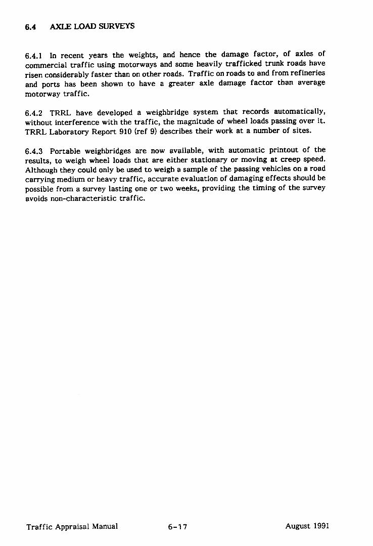
6.4 AXLJZ LOAD SLJRIEYS

6.4.1 In recent years the weights, and hence the damage factor, of axles of commercial traffic using motorways and some heavily trafficked trunk roads have risen considerably faster than on other roads. Traffic on roads to and from refineries and ports has been shown to have a greater axle damage factor than average motorway traffic.

6.4.2 TRRL have developed a weighbridge system that records automatically, without interference with the traffic, the magnitude of wheel loads passing over it. TRRL Laboratory Report 910 (ref 9) describes their work at a number of sites.

6.4.3 Portable weighbridges are now available, with automatic printout of the results, to weigh wheel loads that are either stationary or moving at creep speed. Although they could only be used to weigh a sample of the passing vehicles on a road carrying medium or heavy traffic, accurate evaluation of damaging effects should be possible from a survey lasting one or two weeks, providing the timing of the survey avoids non-characteristic traffic.

k


II

n

InfervIewer ! ROADSIDE INTERVIEW

VEHICLE TYPE

1 2-wheeled m v

2 Car/Taxi

3 Lt9hl Goods Veh

4 HGV (2 Axle)

5 HGV (3 Axle1

. . . . . . . . . . . . .

. . . . . . . . . . . . . .

llr 2 cw/7sm

3 Light Goods Hh

4 HGV (2 Axle)

SHGV (3Aalel

OIhtV

. . . . . . . . . . . . . .

. . . . . . . . . . . . . .

121 I 2-wheeled m v

2 Cw/Tar,

3 C~hl Goods Veh

4 HGV I2 Axlcl

SHGV 13 Axle) BHGV (4 Axle)

Of more

Other

. . . . . . . . . . . . . .

. . . . . . . . . . . . .

131 1 2 -wheeled m ”

2 cwpaxt

3 Lqht Goods Veh

4 HGV II Axle1

5HGV (3 Axle1

6 HGV I4 Axle)

. . . . . . . . . . . . . .

. . . . . . . . . . . . . .

141

NO. OF XXUPANT?

1 8

2 9

3 10

4 II

5 12

6 13 ?

I

1 S

2 9

3 10 4 11

-5 12

6 13 7

I

I 8 2 9

3 10 4 11

5 12

6 13

7

I 1 8 2 9

3 10 4 11

5 $2

6 13 7

DESTINATION (Full Postal Address)

DESTINATION PURPOSE

z-zone COUllly number

. . . . . . . . . . . . . . . . . . . . . . . . . . . . . . . . . . . . 5EdBJc*rb POSlCOd.2

6 Shwvnp . . . . . . . . . . . . . . . . . . . . . . . . . . . I TPW, tlU¶

....................................... NON FREIGH?

Z-.?OiW Cowls 5Educsl0n . . . . . . . . . . . . . . . . . . . . . . . . . . . . . . . . . . . . . . . number

Postcods 6 Shoppmg

. . . . . . . ..a.................. 7Pcrs Bus

. . . . . . . . . . . . . . . . . . . . . . . . . . . . . . . . . . . . . . .

Z-Zone ClXlnty 5 Educrlmn . . . . . . . . . . . . . . . . . . . . . . . . . . . . . . . . . . . . . . number

Poslcode 6 Shovow

. . . . . . . . . . . . . . . . . . . . . . . . . . . . . 7Ferr Bus Frtcnds

No ’ s”eel . . . . . . . . . . . . . . . . . . ..*...............

Town . . . . . . . . . . . . . . . . . . . . . . . . . . . . . . . . . . . . . . . .

z-zone 1 Count” . . . . . . . . . . . . . . . . . . . . . . . . . . . . . . . . . . . . number

Poslcode 6 Shoppq ._.,................ . . . . . . 7 Pets Bus

6 V,s~l Ft,end?l

46 I I I I I I . 9Aec/Lelsure

49 . . . . . , . . 57

jlalton Time Pertod Uumber Date .Sta11

. . . . . . . . . . . . . . . . . . . . . . . . . . . . . . . . . . . . . . . . . . . . . . . . . . . . . . . . . . . . . . . . . . .

ORIGIN ORIGIN (Full Postal Address) PURPOSE

Address Fsm or 1 Home HOU5enPmC..................................~2HOIHOmC

0 Vn~l Ffnnds

. . . . . . . . . . . . . . . . . . . . . . . . . . . . . . . . . . . . . . .

Postcode

6.5 ROADSIDEINTER-G

6.5.1 Advice Note TA 1 l/81 (Traffic Surveys by Roadside Interview - ref 1) recommends standard practice, procedures, site layout, and interview techniques for conducting traffic surveys by roadside interviews. This Advice Note should be regarded as part of this manual (but see below).

6.5.2 The success of traffic surveys by roadside interview depends to a great extent on the voluntary co-operation of the public as vehicle drivers, and the assistance of the police. The use of the standard practice recommended by the Advice Note will cause less inconvenience, greater co-operation from the public and closer co- operation with the police, enabling better and more accurate information to be obtained.

6.5.3 It must be noted that the interviewer has an important role toi play. interviewers can affect the answers and careful training will increase the accuracy of the data.

Coding of Addresses

6.5.4 The Advice Note (ref 1) mentioned above recommends the use of postcodes in the coding of addresses. EEA division now recommends that at least 6 digit Ordnance Survey Grid Reference (OX%) should be used wherever possible. It will probably be found necessary to use 8 digits in the area of the scheme.

6.5.5 It is important that the addresses of origins and destinations in surveys are collected and coded in a manner which allows the survey information to be used, in conjunction with other survey information, by EEA Division (in connection with the development of the National Model), RCUs and Local Authorities.

6.5.6 The aim is to obtain accurate coding of origins and destinations, whether local or remote, to at least 6 digit OSGR. How this is achieved is a matter of local preference and resources. The important thing is that the method should be reliable and accurate. Remote addresses need to be accurately coded so that there is no ambiguity about the location and so that the information can be stored in a form usable by others. It should be noted that the OS Gazetteer lists 6 digits OSGRs for all place names on 1:250,000 series maps. A single reference is given to places such as Birmingham or Bolton.

6.5.7 There are several ways of obtaining 6 digit OSGRs:

i) Code directly to OSGR from addresses using the OS Gazetteer, and OS maps in the study area if more detail is required.


ii) Code directly to OSGR from addresses using the automatic coding method developed by Openshaw and Ramsey. (ref 10).

iii) Code to Post Codes from addresses and then to OSGRs using the Post Code/OSGR file originally developed by the Department and now maintained by the Office of Population, Censuses and Surveys (OPCS).

6.5.8 There is some evidence to suggest that post codes supplied by respondents are subject to error. Careful consideration should therefore be given to whether it is feasible to use post codes without checking them.

6.5.9 If a local ‘study zone’ coding is required this can be combined with a 6 digit OSGR to produce a coding system which is both specific to the scheme appraisal and usable by other parties.

Samnling

6.5.10 The Advice Note contains a small section on sampling size. Appendix D13 discusses the question of estimating the sample size needed to give results to the level of accuracy required in more detail.

Interview Forms

6.5.11 Computer software is being developed which will produce data files from a standard roadside interview from. An example of such a form, with the appropriate punch column numbers is shown at Fig 6.3.

6.5.12 Address coding is acceptable by this software in one of three formats:

i) postcodes;

ii) up to 8 digit OSGR; and

iii) zone code.


6.6 HOME INTERVIEW6

c

6.6.1 A survey interview is a conversation between interviewer and respondent with the purpose of eliciting certain information from the respondent. It may involve leaving a diary or something similar for the respondent to complete at a later stage, eg a travel diary for the following seven days. Whatever form the arrangements take there are three broad concepts which are necessary conditions for a successful interview.

6.6.2 The first is the accessibility of the required information to the respondent. If the respondent does not have the information he cannot answer the question. This may arise because he has forgotten it - this may be important in an interview involving recall of past events.

6.6.3 The second condition is that of understanding by the respondent of what is required of him. The respondent needs to know what is required. He needs to know what is relevant and what is not. It is part of the interviewers job to teach the respondent his “role” in the survey.

6.6.4 The third requirement is motivation on the part of the respondent to answer the questions accurately. It is part of the interviewer’s job to reduce the effect of factors tending to decrease the level of motivation and to build up the effect of those tending to increase it.

6.6.5 Consideration of these concepts shows that the interviewer has an important role to play. They cannot be regarded as merely a means of extracting and recording information. They can affect the recorded answers. One way to increase the accuracy of interview data is by careful interview training.

6.6.6 The coding of addresses is covered in section 6.5. The same considerations apply equally to household as to roadside interview surveys.

Samnle Selection

6.6.7 The first step in selecting the sample is to define the ‘population’ of interest. This will usually be the households or individuals in a particular area. The next step is to decide whether the whole household is of interest or whether it is car drivers, adults, public transport users or some other category.

6.6.8 Having defined the population a list of this population or an approximation to it is needed. The Electoral Register will serve as a list for households or for people over 17/18 years of age. The Valuation List will serve as a list of rateable units, in most cases houses or flats. Both of these lists have their deficiencies. The former is out of date as far as the names of people are concerned but this is not important since the people of interest will normally be the ones living in the area at the time of the interview. It can also undercount households in areas of multi-occupation.


This can be checked for at the time of the interview. The Valuation List suffers from this same deficiency.

6.6.9 Having said this however, as a list of addresses, either will serve. The Electoral Register is probably the easiest to work with. It contains within each Polling District the streets in alphabetical order. If the streets in the area of interest are listed their details can be extracted from the Electoral Register. A recommended procedure for sampling from the Electoral Register is given in an HMSO booklet (ref 11).

6.6.10 Having got the list and decided on the sample size (see following sub-section), the next step ls to select the sample. Ideally, in order for the resulting sample to have reasonable statistical properties, this should be done randomly. However, this is a time-consuming process and the usual technique is to select every nth address where n is selected to give the required sample size.

6.6.11 The technique is as follows: Suppose it is decided to carry out 1000 interviews and that there are 20,000 addresses in the area of interest. Then

R_ 20000 -20 1000

ie every 20th address is used. This is referred to as a ‘sampling interval’ or ‘sampling faction’ of 1 in 20. In order to start the sampling, one address in the first 20 would be selected at random (numbered pieces of paper in a hat, or a table of random numbers) and then every 20th address after that would be selected.

6.6.12 It will sometimes be the case that a ready made sample is already available for the area, from previous traffic work or from other types of market research. Sample survey firms often provide pre-selected samples at modest cost. It should be considered whether such an approach can be used for reasons of economy.

Samde size

6.6.13 There are two calculations that need to be carried out in order to arrive at the required sample size. The first is very similar to that described in the roadside interview section. Decide on the attribute of interest and how accurately it needs to be measured, and then the sample size can be calculated. The Appendix to the Roadside Interview chapter deals with proportions and the formula given is:

9- P(1 -PlQ3

( &)2(Q-1 )+PU-p)Q2 .

where q = required sample size

Q = total flow


6.6.16 If it is not proportions under investigation then something needs to be known (or guessed) about the variance of the variable of interest. If, from a pilot study, or by some other method it is known that the sample variance of the variable is S*, then the required sample size is:

n- S2

[S.E(E) I2

where S.E(3E) is the required standard error of the mean value of the variable under investigation. Eg if it is required to estimate the number of trips per day of a particular type, and it is required that this estimate be accurate to with f a% then SE 0 is known, and knowing (or assuming) something about S*, the required sample size can be calculated.

6.6.17 The subject of sample size is a very large one and it is recommended that if there are any problems the statistician in EEA Division should be consulted.

6.6.18 Having decided the required sample size, it is necessary to allow for non- response by grossing up the calculated sample size. If, for instance the calculations show that 1,000 interviews are required and it is known that about 70% response will be achieved then 1000 interviews (ie 1430) will need to be attempted.

0.7

Questionnaire De&m

6.6.19 There are no hard and fast rules for questionnaire design. The aim is to collect the required information as accurately and efficiently as possible. In most cases, the shorter the questionnaire, the better. It is always worthwhile outlining the table or tables which will be the output of the survey when the questionnaire is drafted: questionnaire design and final data requirements are closely linked.


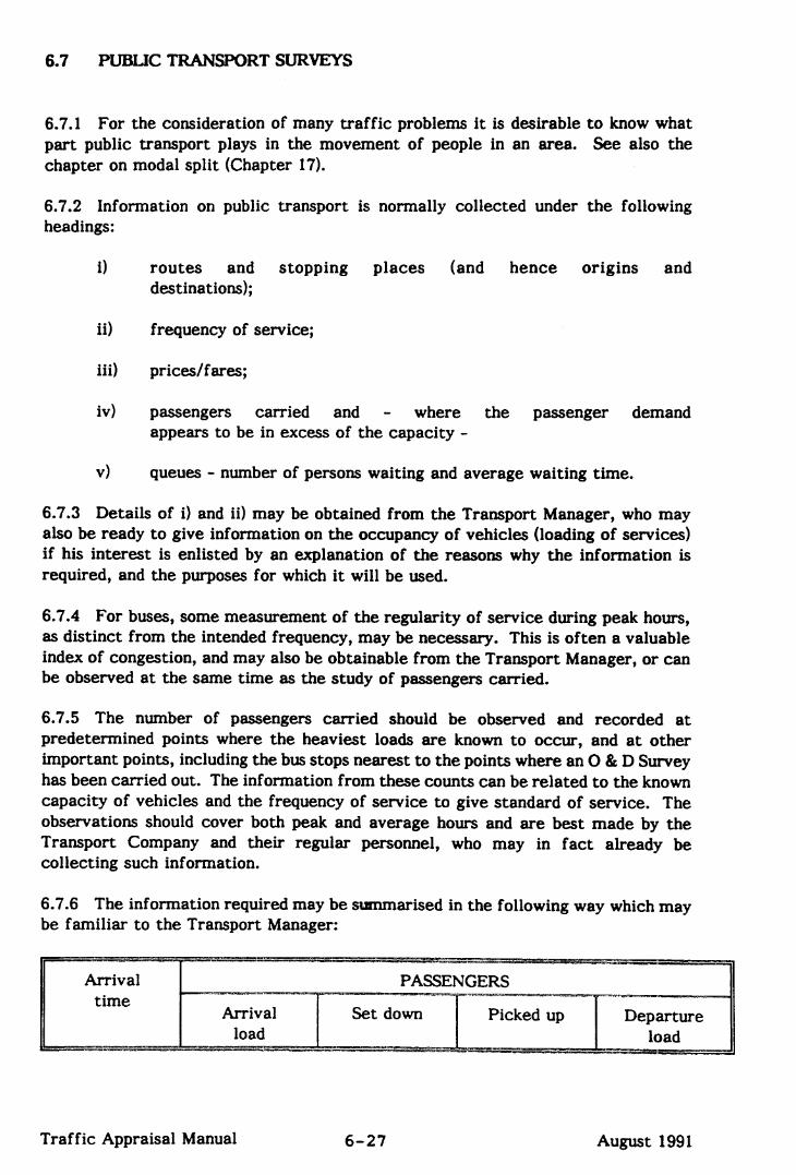
6.7.7 In the relatively few cases where the information cannot be obtained though the Transport Manager, it will be necessary to make special studies.

6.7.8 The number of passengers on single-deck buses can generally be counted by an observer walking along the pavement whilst the bus is stationary. The procedure varies according to the loading as follows:

light loading: count passengers

heavy loading: count empty seats and subtract from the known capacity

loading in excess count number of standing passengers and add to the known capacity

6.7.9 For double-deck buses it will be necessary for the observer to travel a short distance on the bus, and for this purpose it will be necessary to make arrangements with the Transport Manager.

6.7.10 A note should be made of scheduled stops where passenger demand exceeds capacity and the number of intending passengers waiting.

6.7.11 This information will be useful in assessing the density of the passenger traffic at the particular point. The arrival times give the required check on the regularity of service.

6.7.12 Measurements of queues should also be made during peak and non-peak hours. The number of people waiting in the queue should be counted at regular intervals, preferably not exceeding 5 minutes, throughout the hour. The total number of people joining the queue during the hour (=n) should also be noted. The average waiting time or delay in seconds may then be calculated as:

d= 3t600pseconds n

where p is the average number waiting in the queue as given by the periodic counts.

6.7.13 In some areas the effect on road traffic of passengers or goods arriving or departing by rail can be significant. The frequency of rail services, the number of passengers or volume of goods carried and the amount of road traffic generated should be measured, particularly at peak hours. This generated road traffic may of course comprise pedestrians, cars, buses, or goods vehicles.


6.8.8 A problem associated with the collection of partial registration numbers is the possibility that matches may occur between different vehicles, ie spurious matches. These tend to occur where a relatively low proportion of recorded vehicles actually travels between entry and exit stations and where recorded flows are heavy. The number of spurious matches may be estimated approximately by the following formula:

(V-2) ( tfz )

where v= no. of vehicles passing through the entry station

P= the probability of any two partial registration numbers being the same.

(Where these are of the form “123.R” and vehicles have been classified, a typical value of P is 0.000098.)

N= no. of vehicles passing through the exit station

D= difference between the fastest and slowest transit time between entry and exit points (minutes) time

T= duration of survey (minutes)

Z- total number of matches (ie both genuine and spurious)

For a cordon survey, the formula should be applied for each combination of entry and exit stations and the estimate summed over all pairs, although 2 should be set equal to the total matched vehicles at each entry. Provided there is a large element of through traffic, the resulting estimate may be fairly insignificant. There will be a trade-off between the potential error involved and the extra cost of obtaining full registration numbers by automatic methods.

6.8.9 Another benefit of using automatic methods is the avoidance of errors associated with manual recording. In a recent DTp study, involving 10 separate number plate surveys and associated control surveys, only between 88% and 96% of vehicle numbers were found to be recorded correctly, much depending on flow and visibility conditions. Automation may also help to reduce transcription errors and ensure 100% sampling, but may introduce problems of reliability of equipment.

d


6.9.8 If q = average number of vehicles passing through the section in unit time in one direction

X=

Y’

w=

a t

1 =

Q=

D-

then

average number of vehicles counted in this direction when the test car is travelling in the opposite direction

average number of overtaking vehicles less the number overtaken when the test car is travelling in the direction of q

average journey time taken by the test car to travel over the section in the direction of q (hours)

average time taken in the opposite direction (hours)

link length (km)

queue length (km)

delay time (hours)

the average flow q = x + v vehicles per hour a+w

the average journey time of the stream is t = w - y/q hours

the average journey speed of the stream = l/t km/hour

the average running speed = 1_ km/hour 1-D

and average queue speed = Q/D km/hour

6.9.9 A variant of this method is to drive the test vehicle so that the number of vehicles overtaken is the same as the number of overtaking vehicles. The test vehicle is then travelling at the mean speed of the traffic. Timed runs of this kind can serve several purposes and they have been recommended by the Standing Advisory Committee on Trunk Road Assessment. The Department is in favour of including timed runs in traffic studies whenever they are appropriate (see paragraph 6.9.2 above).

Other Methods

6.9.10 Registration Number Surveys are described in section 6.8. By matching the records, and their associated times, it is possible to calculate journey times. However, this method requires a large amount of input to produce reasonable results, and careful thought should be given before it is used.


6.9.18 The average delay to pedestrians in waiting. to cross the road can be found in the same way. The total number n of pedestrians crossing the road is counted and during the same hour an instantaneous count is made at one-minute intervals of those waiting to cross. If p is the average of the one minute counts then the average delay is given by:

d = $600 x D seconds n

There is evidence that the public places greater weight on pedestrian delay than on vehicle delay. Accordingly, pedestrian delay can sometimes be a more important part of a traffic study than vehicle delays.


6.10.7 The ‘road type’ classification of roads is described in the COBA manual. The road types used in COBA are

i) Main Urban

ii) Inter-Urban

iii) Recreational Inter-Urban.

6.10.8 Table 3 in Appendix D14 gives the E-factors (and their coefficients of variation) for converting 12 hour flows to 16 hour flows.

6.10.9 Table 4 in appendix D14 gives the M-factors (and their coefficients of variation) used to estimate AADT from the 16 hour estimate.

Peak Period Factors

6.10.10 Table 5A in Appendix 014 gives for the ‘road type’ classification used in COBA (see above) factors to convert from: AADT and AAWT to PHF (peak hourly flow) and the 10th 3Oth, SOth, 100th and 200th highest hour. Table 5B gives the corresponding coefficients of variation.


Traffic Appraisal Manual November 1997

CHAPTER 7 : WITHDRAWN

(was NATIONAL SUB MODELS)

The National Trip End Model, its underlying planning data projections and car ownershipforecasts, and its relationship with the National Road Traffic Forecasts, are fully described inDMRB v12.2.3.

CHAPTER 8: THE PRODUCTION AND CALIBRATION OF A BASE YEAR TRIP MATRIX

8.1

8.2

8.3

GENERAL

MATRICES FORMED BY EXPANDING OBSERVATIONS

FITTING SYNTHETIC TRIP DISTRIBUTION MODELS OF THE GRAVITY TYPE

8.4 THE USE OF MODEL ELEMENTS IMPORTED FROM OTHER STUDIES

8.5

8.6

8.7

8.8


ESTIMATING MATRICES FROM TRAFFIC COUNTS

DISAGGREGATION TECHNIQUES

MERGING DATA FROM DIFFERENT SOURCES

MATRIX MANIPULATION


CHAPTER 8: THE PRODUCTION AND CALIBRATION OF ABASE YEARTRIPMATRIX

8.1 GENERAL0

Introduction

8.1 .l This chapter is concerned with the production of the base year trip matrices which form the foundation for the forecast year trip matrices used in scheme appraisal. It may be assumed that a study area has been defined and a compatible scheme zoning system and network developed (chapter 3); the choice of model form will have been made (chapter 51, and the data necessary to construct the chosen model obtained (chapters 4 and 6).

8.1.2 Where the assessment of a scheme necessitates the use of a complex, matrix- based model, it will generally be necessary to create base year trip matrices for that scheme using whatever existing sub-models and data are appropriate, supplemented by local data. Trip matrices from the RHTM project, or from the revised National Model, or from a regional model, or a model from an adjacent scheme, should however be used where this would be cost effective, and where the trip matrix can be validated adequately in the area of interest (see chapter 11).

8.1.3 A reasonable estimate of longer distance movements is available from the National Model of long distance movements. The calibration and validation of this model has been reported to SACTRA (ref 9). The main use of data from this model will be in survey design, but the estimates of long distance traffic from the model may be used in a local model, and should be seriously considered where much new survey data would otherwise be needed. As usual, it will be necessary to validate this external data in the context of the particular problem in hand. Further information on the development and use of the National Model is available from EEA in the form of the National Model Report and the National Model User Guide. The validation of the National Model is reported in section 11.5 of this manual. The data available from the National Model is described in section 4.2.

8.1.4 A number of methods are now available, and acceptable, for producing base year trip matrices. The aim of this chapter is to describe good practice, document recent advances in technique, and advise on the circumstances in which the various methods are appropriate.

8.1.5 Two methods of preparing base year trip matrices are described:-

i) trip matrices which contain only expanded observed trip data (sometimes known as a saturated model);

ii) synthetic trip matrices produced by gravity trip distribution models which may include input from sub-models of either local or national derivation. The case for replacing model estimates with sampled observed trip data is also considered.


Whilst other trip distribution models are available, they are not often appropriate for trunk road appraisal. But EEA Division would be pleased to discuss any proposal to use an alternative model form for a particular scheme.

8.1.6 After describing the acceptable model forms, the chapter covers the disaggregation of trip matrices to a finer level of zoning and the merging of trip matrices from different sources. The chapter concludes with a description of the matrix manipulation software that is available and its use in the formulation of the trip matrices for input to assignment models.

The Selection and Treatment of Trio Fbmoses. Vehicle TYDCS and Time Periods

8.1.7 The recommended trip purpose and vehicle type combinations for which individual trip matrices should normally be produced for assessment purposes are:-

Cars and Vans - Journey to/from work Cars and Vans - On Employers Business Cars and Vans - All other purposes Goods Vehicles - All purposes

Vans are defined as all commercial vehicles of less than 30 cwt (1.5 tonnes) unladen weight, that is commercial vehicles with only 2 axles and with a total of 4 tyres on both axles.

Vans are classified by trip purpose and grouped with cars because their private use and impact upon assessment are similar to private cars. However, limitations in current forecasting techniques require that matrices of cars on employer’s business are developed and stored separately to those of vans on employer’s business (see 12.3). Goods vehicles are all commercial vehicles of greater than 30 cwt (1.5 tonnes) unladen weight, that is, commercial vehicles with more than 2 axles or with more than 4 tyres on 2 axles. Where there is a very high proportion of goods vehicles, particularly very heavy goods vehicles with 4 axles or more (about 25 tonnes or more) or where there is a high proportion of longer distance trips, consideration should be given to modelling these very heavy goods vehicles separately to ensure that they are adequately considered in the scheme assessment. This is necessary because these very heavy goods vehicles have a high predicted growth rate and this could impact upon design considerations. The public are also more aware of very large lorries and the effect they have on the environment. Where it is thought necessary to model very heavy goods vehicles separately, special attention should be paid to sampling from this vehicle category to ensure that adequate data is collected, as absolute numbers will be relatively small.

8.1.8 Current assessment methods do not utilise all of the above trip purposes and vehicle type combinations separately: however, changes are in the pipeline which are expected to do so in the medium term future.

8.1.9 When using a synthetic trip distribution model to produce trip matrices, it may well be necessary to model more trip purposes than the above in order to reflect adequately differences in trip making behaviour.


k,

Home-based trip purposes are usually treated in a different way to non-home-based trips. By convention, every trip to or from a home base is considered as if it started from home. The ensuing home-based trip matrices have to be converted into genuine origin and destination trip matrices prior to assignment by a process of matrix manipulation (see 8.8). The vehicle types and trip purposes modelled will depend upon the data to which the models are to be fitted: the minimum number which reproduce the variation in the observations being adopted.

The Selection of Time Periods for Daily Matrices

8.1.10 This chapter is concerned with the preparation of a base year matrix of trips between zone pairs which is the best estimate of the number of trips between each zone pair for the time period covered by the matrix. Recent work on the assessment of errors has resulted in an understanding of the need to pay new attention to:-

i) the time period for which traffic models are built; and

s

ii) the way in which the outputs required for scheme assessment are derived using factors (which may carry appreciable error) to convert data from one base to another.

8.1.11 The end product of a traffic appraisal is the link flows used in scheme assessment, a major requirement being the 24 hour AADT link flow estimates used in economic appraisal. Trip matrices are an important intermediate component in estimating link flows, and can be of considerable descriptive value in operational appraisal. However, robust quantitive estimates of trip movements (divorced from the roads on which they take place) are not directly necessary for environmental or economic appraisal (in COBA or NETBEN), or for other elements in the assessment framework.

8.1.12 If factoring takes place at too early a stage in the analysis of traffic data, the uncertainty of the factor will be added to that of the sampled data itself, and this could have an adverse effect on some potential future uses of the data - particularly in model validation or when merging trip matrices - and on the ability of the model to discriminate between alternative schemes. During model validation, for example, observed and assigned link flows, each of which has a tolerance, will be compared. The tolerance on the link flows will be much greater for an estimate of 24 hour AADT flows than for an estimate of flow during the survey period in which interviews took place (due to the uncertainty of the factors used - see 10.7, for example). This wider tolerance makes it much more difficult to distinguish the statistical differences between observed and modelled flows.

8.1.13 As a consequence, the time periods recommended for model building are:-

i) For models based upon expanded the interview period of the observations major data set (eg 12 hour

September Weekday);


ii) For synthetic trip distribution - models using trip end estimates from the national trip end models as a calibration constraint in the base year.

24 hour Annual Average Weekday Traffic (AAWT)

8.1.14 Traffic estimates required for time periods outside the modelled period can be obtained by factoring link flows after assignment (eg 12 hour September weekday to 24 hour AADT) as described in Section 6.10. A major result of this approach is that when interview period models are built, because the accuracy of an estimate of 24 hour AADT is very similar when based upon a 12 hour link flow or a 16 hour link flow (refs 1 and 21, the shorter time period can be adopted without compromising the quality of the information produced. The recommended period for interviewing for models based upon expanded observations becomes a 12 hour weekday (7 am to 7 pm, Monday to Thursday) during the months of April, May, June, September and October (the so-called “neutral” months for which the conversion factors to give annual average daily traffic flows have the smallest coefficient of variation).

8.1.15 When using a synthetic trip distribution model with an estimate of the 24 hour annual average weekday trip ends from the national trip end models, the observations from the interviews will have to be factored to represent 24 hour annual average weekday movements prior to input to the trip distribution model calibration. This involves two steps:-

i) factor the interview period observations to the total 24 hour classified count using site specific factors dependent upon the vehicle class of the interviewed vehicles; and

ii) factor each interview from the 24 hour interview day to represent 24 hour annual average weekday movements.

Conventionally, roadside interviews of 16 hours duration (6 am to 10 pm) have been used here. It is not known whether the use of 16 hour interview information gives a substantially more accurate picture of the number and distribution of trips in the 24 hour annual average weekday than would 12 hour interviews. Neither is the effect upon the final output, the 24 hour annual average daily traffic flows, known (these areas may be investigated by EEA in due course). In the absence of further information, interviewing for longer than 12 hours may be considered where a 24 hour annual average weekday model is to be built.


8.2 MATRICES FORMED BY EXPANDING OBSERVATIONS

8.2.1 The simplest way to produce a trip matrix is to form it directly from expanded observed trip records. This may be termed a saturated model with one observation for each parameter estimated. Matrices of this type may be used:-

i) in their own right for scheme evaluation purposes; and

ii) as an input to synthetic trip distribution models.

8.2.2 All that is required to build an observed data trip matrix is a file of trip information with the trip origins and destinations coded to the scheme zones. Each trip record is read in turn and the number of trips represented by each interview is calculated by expanding it on the basis of the factors appended to the records, eg the proportion of interviewed counted traffic in the time period. The resulting number of trips is accumulated with all other records sharing the same origin zone and destination zone in the matrix cell defined by the origin zone (row number) and destination zone (column number)

82.3 Trip matrices formed directly from expanded observations will contain an estimate of the total numbers of those movements intercepted by the survey. They will only contain an estimate of all the trip interchanges between each zone pair if the survey has included interviews on all possible routes between all the zones (saturation interviewing). This would be an expensive procedure which is not recommended. Similarly, traffic within each roadside interview cordon will not have been sampled unless household interviews were carried out within the cordon. A diagram illustrating this is at figure 8.1.

8.2.4 When using an observed data trip matrix as input to a synthetic trip distribution model, it is imperative that only those movements which have been fully surveyed (ie where interviews have been conducted on all the possible routes between the zones) are included in the input trip matrix (such movements are usually called “fully observed” movements). This is because every cell value in the input trip matrix is treated in the calibration process as though it were fully observed and the inclusion of any partial data would bias the model fitted to the data.

8.2.5 A trip matrix formed from expanded observations will contain (often a fairly large proportion of) cells with a zero value, indicating that no trips between these particular zone pairs were intercepted by the survey. The zero cells may be of two types:-


FIG 8.1

MOVEMENTS OBSERVED BY INTERVIEWS

) Roadside interview Cordon only

B-B lnlervaew

i D

Only trtps which cross the Intervtew Cordon WIII be surveyed as lollows -

Internal to External frlps - A-A - fully surveyed;

Internal to Internal trlps -B-B - not surveyed :

External to External trips -c-c - not surveyed : but

Some External to Externai trips - D-D - may be partially surveyed

ij Roadside Interview Cordon surrounding a Home Interview area

D

A-A

t

-I---

c-c

Home lnlerv8ew

Area Roadsde lnlervtew

i

Cordon

B-B

I f D

Internal to External trips - A -A - fully surveyed tn roadside IntervIews. all trips by restdents surveyed In home lntervlews

internal to Internal trips -B-B- all trips by resrdents surveyed In home tntervlews.

External to External trips -C-C - all trips by residents surveyed In home Interviews.

D-D - may be partially surveyed In roadslde IntervIews


i) structural zeros - where both zones are outside, (or with roadside interviews inside) the interview cordon, the survey is unlikely to intercept any trips between the zones - eg an interview cordon around London is unlikely to intercept any trips between Birmingham and Nottingham; and

ii) observed zeros - where one zone is within the interview cordon and the other without (or both within with household interviews), the trips between the zones will have been fully surveyed (ie all the trips between then will have been included in the total population from which the interview sample was drawn) but, by chance, none were intercepted in the sample interviewed. For example, a roadside interview cordon around London would include within the total population of trips from which the interview sample is drawn the one trip (say) which took place on the day of the survey between London and Penzance, but if this vehicle was not stopped at an interview station (perhaps a 3 in 4 or 75% chance) no trips between London and Penzance would be recorded.

In a sense, these are “phoney” zeros because in neither case does a zero cell entry guarantee that there were no trips between the zones during the survey period.

8.2.6 The ROADWAY suite program which builds trip matrices from a file of individual trip records is called RDMVAR. The trip data file input to RDMVAR is prepared by either RDRISP, for data from roadside interviews, or RDHISP, for data from household interviews. These programs select trips of the required trip purpose and vehicle type combinations and produce a file of trip records with the data arranged in the most efficient from for inputting to RDMVAR.

8.2.7 RDMVAR includes an option to construct a matrix containing the index of dispersion (the variance to mean ratio) for each observed cell calculated from sampling theory, including that of the observed zeros. The calculated index for a cell is the effective scaling up factor for observed trips in the cell, allowing for uncertainty in the various scaling up factors as well as the sampling process itself. For the observed zeros, the average effective scaling up factor for the complete survey is adopted. The methodology used is described in chapter 10 and in the program documentation. This information is needed to assess the accuracy of the observed cell values, of aggregations of cell values into sectors and corridors, and, ultimately, of assigned link volumes. The relative accuracies of observed data trip matrices can also be taken into account when matrices are combined. All of these areas are more fully explored in section 8.6 and in chapter 10.


8.3 FITTING SYNTHETIC TRIP DMRIBUTION MODELS OF THE GRAVITY TYPE

General Princioles

8.3.1 The gravity model is the name given to the form of synthetic mathematical trip distribution model most often used in transportation studies in this country. Put simply, the model states that the chance of a visit to a town is proportional to the size of that town and the inverse of the intervening distance.

8.3.2 A fully synthetic trip distribution model provides a full matrix of trips between all the zones in a given zoning system without the need for saturation interviewing (see 8.2). It uses a mathematical model to calculate how many trips will be made between each zone pair, the parameters of the model being derived from a sample survey. A full matrix of trips is required to provide estimates of the total traffic flows on all roads in the study area, although this level of detail is only needed in exceptional circumstances. A further benefit of using this modelling

technique (see below) is that the model can be used in the forecasting mode to predict the traffic flows likely to be generated by a development to a “green field” site, or a major network change such as an estuary crossing, where substantial changes to the existing trip pattern can be expected.

8.3.3 The equation chosen for the gravity trip distribution model is typically of the form:-

t ij = a; bj f(Cij)

where tij is the number of trips from zone i to zone j,

ai is a factor associated with travel from zone i,

b_i is a factor associated with travel to zone j,

‘ij is the “cost” of travel from zone i to zone j, and

f(Cij) is a measure of the resistance to travel on the highway network between zones i and j.

8.3.4 Mathematical models of this type use simple mathematical equations to describe human behaviour (which is anything but simple). Equations are used to represent the way in which people behave, on average, without any attempt to relate the figures to an individual’s trip making or destination choice. The basic model can be elaborated in the following ways:-

i) the segregation of data for different vehicle types and trip purpose combinations to which individual models are fitted, thus allowing for variations in trip making behaviour; and


ii) the incorporation of different functions (f) depending on the characteristics of the origin and destination zones. This allows movements made inside a town, and travel from that town to other areas to be treated separately should the input data support such action.

8.3.5 The process of estimating the parameters of a gravity trip distribution model, using the characteristics of an observed trip matrix and a road network, is known as calibration. The process is iterative with successive updating of the row, column and cost factors (function values). The parameters obtained from the calibration process may then be used to predict the number of trips which take place between each zone pair, and a complete trip matrix emerges. This trip matrix is a fully synthetic matrix and is known as the base year forecast trip matrix.

8.3.6 The ROADWAY suite program which calibrates gravity trip distribution models is called RDGRAVZ. Details of the program are contained in documentation available from Highway Computing, division (HC). A further description of the facilities available within RDGRAVZ is to be found later in this section. Other commercially available programs may be equally suitable for most applications.

8.3.7 When calibrating trip distribution models, the resistance to travel between zones should be measured in “generalised cost” units. Generalised cost is a weighted combination of the time taken and the distance travelled between zones. In more complex models, it may also include other elements such as terminal costs (parking charges etc). The generalised cost of travel between each zone pair should be measured along a single route through the road network chosen to minimise the generalised cost of travel through the network. Routes may be obtained using the ROADWAY program RDSKIM which will output a matrix of the generalised cost of travel between each zone pair, generally known as a “skimmed tree” matrix. The generalised cost of travel will be calculated either in monetary units (pence) or in time units (minutes).

8.3.8 The coefficients for use in the generalised cost equation vary with different trip purpose and vehicle type combinations. The recommended coefficients are published in the current version of Highways Economics Note 2 (HEN 2) which is reproduced in appendix 8.1. Where the routes selected for assignment are not obtained by minimising the generaiised cost using the coefficients recommended in HEN 2, consideration should be given to whether the generalised cost values obtained from the assignment routes would be appropriate for trip distribution purposes. This is particularly relevant to the modelling of commercial vehicles where route choice studies suggest that lorry drivers do not always seek to minimise operating costs. EEA division would be pleased to advise on any problems encountered in this area.

8.3.9 To assist in the fitting of gravity trip distribution models, a program has been developed to compare a synthetic trip matrix with the observed trip matrix from which it was developed. This program is called RDCOSM. The program calculates a number of statistics based upon the residual errors in the fitted model, ie the difference between observed and modelled values for the observed cells. It is envisaged that this program will be of use to practitioners in the fitting of gravity trip distribution models by helping to identify which of a number of trial fitted models most accurately reproduces the input data.


L Calibratinc Partial, Map-@, ,.‘&chpiauq

Comparative statistics of this kind are still experimental, however, and advice on the use of RDCOSM will be available from EEA.

8.3.10 Having described the general principles of gravity trip distribution models, the following sections describe more fully the different methods available for calibrating these models. The following methods are described:-

i)

ii)

the partial matrix method; and

other methods of calibration, including:-

a.

b.

C.

estimating the base year matrix as a prediction;

the synthetic trip end technique; and

a combination of the partial matrix and synthetic trip end techniques (sometimes know as the “Top-L” method).

8.3.11 The input data required for a partial matrix calibration includes an observed trip matrix, containing the trips from those movements which have been fully observed in the survey (see 8.21, and a matrix of the generalised cost of travel between each zone pair, which is known as the skimmed tree matrix. The technique is named after the “partially observed” trip matrix which is the major input to the calibration.

8.3.12 The steps in carrying out a partial matrix calibration are as follows:-

i) prepare the input observed data trip matrix (see 8.2) and the skimmed tree matrix and submit these to the gravity model calibration program;

ii) the program makes a first estimate of the value of the column and cost factors and computes for each row the factor which satisfied the row constraint: at the same time the sums required to update the column and cost factors are accumulated. At the end of each pass through the matrix (known as an iteration) the column and cost factors are updated. This process is repeated until a pre-set number of iterations have been completed or until any specified closure statistics have been satisfied; and

iii) a trip matrix is then computed using the row, column and cost factors fitted during the calibration. The output is a matrix with a synthetic estimate in each cell known as the base year forecast matrix.

8.3.13 The constraints satisfied by a partial matrix estimate are:

i) modelled and (grossed-up) observed trip numbers will agree for each row and column; and


ii) for an exponential cost function, modelled and observed mean trip costs will be the same. For a Tanner (two parameter) cost function, modelled and observed mean trip costs, and mean logarithms of trip costs, will be the same. For an empirical (tabular) function, the

modelled and observed number of trips will agree in each cost band.

8.3.14 RDGRAVZ, the ROADWAY suite program which calibrates gravity trip distribution models, includes the facility to fit a base year trip matrix using the partial matrix technique. With Poisson sampling for the trips in each cell (ie random sampling from an infinite population), partial matrix fitting is maximum likelihood estimation when the sampling fractions (expansion factors) are the same in each cell. If the sampling fractions vary (the true case with household and roadside interview data) it is similar, but not identical to maximum likelihood. The fitting method may be interpreted as minimising the discrepancy between modelled and observed values, with the discrepancy measured in a particular way (which, for small discrepancies, is like the Chi-squared measure).

8.3.15 RDGRAV2 is a modified version of an earlier program. The modifications provide Monte Carlo estimates of the variance of the fitted model parameters due to sampling errors. This is achieved by first fitting the model to the observed data to obtain a “reference” trip matrix. From the reference matrix random samples of the cell values are drawn in a way similar to the real sample. Each synthetic sample is fitted, and the variance of the model parameters calculated from these independent estimates. The use of this information is discussed in Chapter 10. RDGRAV2 is now available.

8.3.16 The adequacy of a calibration to a partial matrix of trips, as measured by the accuracy of the fitted model’s estimates, depends for a well fitting model upon the number of sample counts (that is unexpanded trips) in each row, column and cost band. The method will give zero estimates for a row or column in which there are no observations, and clearly cannot give an accurate estimate if the number of observations is very few. Thus, the whereabouts and amount of data should be chosen to achieve sufficient sample (unexpanded) trips in the partial row and column totals and the cost function values to which the model is fitted.

8.3.17 One of the problems encountered when calibrating gravity trip distribution models using the partial matrix technique is that the model estimates for the unobserved cells may not converge to a unique solution. The estimates for the observed cells will always be unique. Estimates for the unobserved cells are obtained from the factors fitted in the calibration. If the pattern of observed cells is sparse in an unfortunate way, it can happen that there is more than one set of factors which give the same estimates in the observed cells but different values in some of the unobserved cells (ref 3). When this “non-identifiability” occurs, the results in the unobserved cells are essentially arbitrary (depending upon accidental details of the starting values and how the program operates). This will not occur if there are enough occurrences of each cost band in different rows and columns of the observed cells, or if an analytical (exponential or Tanner) function is used. It is also unlikely with a smoothed empirical function, such as those produced by the monotonically decreasing or cubic spline automatic smoothing options included in RDGRAV2.


8.3.18 A method of checking whether the conditions which cause “non-identifiability” exists in a particular case has been proposed. Essentially, this involves solving the problem twice from different starting points to see whether the row, column and cost factors differ. The facilities to enable this may be included in RDGRAVZ in the future.

8.3.19 Advice on the amount and location of the data necessary to a satisfactory partial matrix calibration is expected to follow the completion of a research commission. The best advice currently available is that the proportion of observed cells should be reasonably high (a minimum of about 70%) and the input data should be well dispersed over the matrix. In effect, it may be safer to collect a small

amount of data for many O-D pairs rather than much data for a small number of O-D pairs.

8.3.20 The major benefit of this method is that a full base year trip matrix can be synthesised from trip information collected at roadside interview stations, thereby avoiding the costly process of collecting household interview data and calibrating car ownership and trip end models. Once again it should be emphasised that this base year trip matrix is a base year forecast derived using the model parameters calibrated against the input data and does not contain the input data itself. Advice on when, if ever, the observed trip data is to be preferred in use to the model estimate of the same movements will be given when the results of a current research commission are available.

Other Methods of Calibration

8.3.21 It has been found in practice that the estimates given by the partial matrix technique for the unobserved cells - and thus for trip end estimates in partially observed rows and columns - can be relatively unreliable. Whilst this problem can be reduced by a well-chosen spread of data over the matrix (see 8.3.151, the adequacy of the estimates for the unobserved cells is conditioned by the assumption that the model is not only a good “fit” for the observed cells, but also, in a sense, a good “fit” for the unobserved cells. In practice, of course, it is difficult to ensure that such a condition holds in advance.

8.3.22 Practitioners have therefore attempted to control what, under the partial matrix technique, might have been unacceptably inaccurate estimates in the unobserved cells, by allowing externally derived estimates of trip-end totals (taken from a trip end model) to affect the result of the distribution model. this has been achieved in one of three ways:-

i) estimating the base year matrix as a prediction using the deterrence function from a prior partial matrix calibration to distribute the base year trip ends predicted by the trip end model (sometimes known as the two-stage process);

ii) the synthetic trip end method, where the model is calibrated directly to the trip ends predicted by the trip end model using the characteristics of an observed trip matrix; and


iii) a development of the synthetic trip end technique which uses synthetic trip end constraints for selected zones and partial observed trip ends as a constraint for the remainder (sometimes known as “Top-L” calibration). This method is fully described in ?

All these methods may be executed by the ROADWAY program RDGRAV2.

8.3.23 Whilst all these techniques have the advantage of using essentially only minor adaptations to the iterative procedures used for the partial matrix technique, they all suffer from the disadvantage that, unlike the partial matrix technique, they are not underpinned by a sound statistical methodology in that no formal minimising function has been defined for them, and other inputs (for example the trip end estimates) are taken to be “correct” when they are in fact subject to the errors of estimation. It would be more appropriate to use an estimation procedure, such as maximum likelihood, in which simultaneous account is taken of the numbers of trips in the observed cells and their error distribution. The principles and procedures necessary to achieve this have been assessed by Kirby et al at the Institute for Transport Studies, the University of Leeds, and what has come to be known as the “combined estimation procedure” has been propounded (ref 4). This procedure has not been further developed, or tested, and no software is available which incorporates it. Consideration is being given by EEA to further development of the procedure.

8.3.24 The following paragraphs describe the three techniques outlined above. EEA division will be happy to advise on the validity of other proposed methods of calibration.

Estimating the base year as a medict.

8.3.25 This is a two-stage procedure:-

i) estimate the parameters (a;, bj and f(C)) of the gravity model by fitting to an observed trip matrix using the partial matrix technique; and

ii) take the deterrence function, f(c) from this calibration and use it, unchanged, to distribute an estimate of the row and column trip ends.

The output trip matrix, if the trip end estimates represent the base year, is an estimate of the base year situation produced as a prediction. This technique will control the ‘wilder’ estimates of trips in the unobserved cells, probably at the cost of a less good fit to the observed cells. When this technique is to be used to forecast future year flows (by inputting future year trip end estimates) the base year trip matrix estimated as a prediction is the trip matrix which must be validated (chapter 11) as that upon which future year trip matrices will be based.


The synthetic lri~ end method.

8.3.26 This technique is a single stage procedure with an observed trip matrix and an estimate of the row and column trip ends being input simultaneously to a single calibration and trip matrix production run. This procedure allows the trip end

estimates to influence the values of the fitted deterrence function, f(C). The number of parameters fitted in this model does not permit the constraints of the absolute number of trips in each row and column and the absolute number of trips in each cost band of the deterrence function to be satisfied simultaneously, there being one factor too few in the model to be fitted. To overcome this, one of the constraints must be relaxed, or made relative rather than absolute. Thus, either the constraint of the number of trips in each cost band of the observed trip cost distribution is relaxed (the shape being maintained but the absolute number of observed trips in each cost band of the trip cost distribution not being reproduced by the model), or the trip end constraint is relaxed (the total number of trips in the matrix being allowed to alter to the number required to satisfy the absolute number of observed trips in each cost band of the observed trip distribution). The relative adjustment should be small in either case if the model is to be considered an adequate fit to the data. The problem of non-identifiability (see 8.3.16) is not thought to arise with models fitted using the synthetic trip end technique.

TOD-L” calibration

8.3.27 This method is a development of the synthetic trip end technique, in that the model is fitted such that a number of aggregate quantities from the input data are exactly reproduced by the fitted model. In this case the aggregate quantities are the total row and column trips ends estimated by the trip end models where these are applied (as in the synthetic trip end method), the number of trips in the observed cells in the remaining rows and columns (as in the partial matrix method), and the number of observed trips in each cost band of the trip cost distribution. As with the synthetic trip end technique, this method has more independent constraints than variables unless additional factors are introduced. In this case two are required which may apply either to the internal trip end model attractions and generations (leaving the observed data intact), or to the observed data and the attraction trip ends (leaving the trip end generations intact). The method, which enables a trip matrix to be developed for a study area which is not bounded by an interview cordon but for which some trip information is available, reduces the amount of new survey data required by removing the need for an interview cordon around the study area, whilst allowing the incorporation of existing observations within the study area. Movements between zones outside the study area (external to external movements) may be supplied by an external model (such as the revised national model mentioned in section 8.1) or from expanded observations - the estimates produced by the model for such external movements should only be used with caution (see 8.3.20). The model requires as input an observed trip matrix, a matrix of the travel cost between zones, and the zonal trip ends for those rows and columns to which the synthetic trip end constraint is to be applied.


8.4 THE USE OF MODEL ELEMENTS IMPORTED FROM OTHER STUDIES

General

8.4.1 The range of existing traffic models available throughout the country includes local town and county models developed by Local Authorities, regional studies carried out by Department of Transport or bodies such as the British Airports Authority, and those developed during the Regional Highway Traffic Model (RHTM) project and the National Model of Long Distance Movements which cover the whole country. Clearly, it is sensible, and cost effective, to utilise existing models for the

assessment of trunk road proposals where these models can be demonstrated to be adequate for the purpose. Whilst ultimately, this will rest upon the results of

validation tests described in chapter 11, there are several technical and other issues which must be considered.

8.4.2 The use of an existing model will reduce the costs of data collection (surveys) and model production. Less tangible, though no less real in the local context, are the benefits of close liaison with the planning authority concerned and the use of common data for local and Departmental decision-making, leaving only the interpretation of results to be debated.

8.4.3 On the other hand a number of problems are likely to arise from a decision to adapt an existing model. The greatest of these is that the model will not have been produced with a particular trunk road scheme in mind, but for some other specific purpose. A number of ways in which this could manifest itself include:-

i) the model structure could be too fine or too coarse in the study area for the trunk road proposal, with too much, or too little, detail elsewhere;

ii) the model could include alternative modes of travel which are not effected by the trunk road proposals, leading to additional model operating costs;

iii) the local model is likely to have been quite properly calibrated and validated with the town centre problems in mind. The trunk road proposal, by the very nature of trunk roads, is likely to be in the periphery of the town. The result could well be that the trunk road assessment will rely upon elements of the model which are of secondary importance to the local study and to which little attention has been paid in the model calibration and validation;

iv) vehicle type and trip purpose definition could have been used which do not accord with the standards laid down in chapter 6 of this manual;

v) the error structure of the data upon which the model is based may not be known; and

vi) the standard errors of the estimates of the model parameters may not be known.


8.4.4 With these potential problems in mind it is recommended that any existing model which is being considered for incorporation into a trunk road study should be subjected to an audit to confirm its integrity for trunk road appraisal purposes before the decision to use it is taken. The audit should pay particular attention to the data base of the model, its specifications and the documentation available to support the model calibration. The objectives of the audit will be to ensure that the model calibration has been carried out in accordance with good practice (such as laid down in this manual) and to confirm that the model is suitable for the proposed purpose. However, it would not be sensible to apply this policy generally to those trunk road studies which are already completed or well advanced.

8.4.5 The final hurdle, as in the case of all models to be used for project appraisal, is an acceptable validation of the model output by comparison with independent data (ie data which has not been used in the model calibration). The procedure for validation is described in chapter 11, Model Validation.

8.4.6 Where an existing model is based upon observations taken more than about 6 years ago, it is recommended that the forecasting procedure to be used should be tested by forecasting to the present day and comparing the model estimates with recently collected data.

8.4.7 These are general considerations which relate to all models. The approach will vary slightly depending upon which model elements are to be imported; these differences are discussed in the following sections.

Models Develoned During the Regional Highwav,.Traffic Model Row

8.4.8 It may be appropriate to use the models developed during the Regional Highway Traffic Model (RHTM) project for particular schemes, and consideration should always be given to this possibility. The Standing Advisory Committee on Trunk Road Assessment (SACTRA) has examined this project (ref 5). A conclusion of their report was that “local teams should be encouraged to use the data and sub- models developed as part of the project wherever it can be demonstrated that they are well validated for the scheme being investigated” (recommendation 6).

8.4.9 The national car ownership and trip end models described in sections 7.2 and 7.3 have been developed using the car ownership and trip end models from the RHTM project. In order to minimise the amount of survey work needed, it is recommended that the use of these models is always considered (but see Chapter 7) before the preparation of locally derived trip end models is undertaken.

8.4.10 The base year private vehicle trip matrices obtained during the RHTM project have not been further developed since the project ended in October 1979. The preparation of these matrices is catalogued in a selection of RHTM reports (refs 4, 10-13). These base year trip matrices may be used in scheme appraisal where this would be cost effective and where they can be shown to validate adequately in the context of the particular study. Details of the availability of these matrices are in appendix 20.1.


8.4.1 1 SACTRA commented upon the RHTM base year commerciaI vehicle matrices in the following way: “We conclude that the matrices are the best infumstfon available on commercial trips at the national level fur the base year, and recommend thst they should be available for scheme assessment, subject to checks of their validity in the area being studied’’ (recommendation 16). The calibration of the base year commercial vehicle trip matrices is described (ref IO). Details of the availability of these matrices are also in appendix 20.1.

8.4.12 The suwey data coIlected during the RHTM project has been archfved. Full details of the data and its availability are given in chapter 4, Existing Data Sourcm.

8.4.13 Local: car ownership and trip end models should have been calibrated tu local conditions, but a check on the integrity of the calibration should be made to support their use in representing the base year situation. A major difficulty arises when local sub-models are used for forecasting but the problem can be Overcome by imposing cootrd totals of future vehicle kilometres derived from national sources, This effectively restricts the local model to a distributive role. This is further described in chapter 12.

8.4.14 A problem which is often encountered in local models is the incorporatfun of independent variables which are difficult to forecast. Urban studies with small zones and highly disaggregated purpose splits are particularIy vuherabk in this respect with trip end models calIing for predictions of land use parameters which are difficult to measure in the base year, let done forecast fur years ahead. ExampIes of such parameten are number of education places, floor areas of retail outlets and the availability of recreational facilities, each of which might be required at a zonal IeveI. The sensitivity of mod& which require such detailed inputs should be explored by sensitivity testing so that the scheme assessment can take accuunt of the possible outcome should local aspirations not be fulfilled.

TriD Matrices from ExternaI Models

8.4.15 In common with any other trip matrices, those developed fur use in local studies cannot usualIy be given an overall dassificatlon of either good or bad in their representation of the true situation, but will prubabIy be good in some parts and bad in others. I t is important, therefore, to identify those areas of the trip matrix which are particularly relevant to the trunk road appraisaI at hand, and to concentrate upon those matrix elements when consideringwhether or not a model is adequate for the intended purpose.

8.4.16 Problem arising from external matrices are usually related to the scale or structure of the model. If the zone system and network are compatible with the local objectives, then the central 8rea of the town, say, wiII be modelled to a very high level of detail. This will have two consequences: firstly, the model will be more costly to use and, secondly, the relief to the network from an investment is likely to be widely distributed over a fine netwurk.

Traffic Appraisal Manual 8-7 9 August 1991

This may well be more realistic - as traffic reverts to the main road from rat-runs - but i t makes the benefits due to the new road difficult to quantify and to present to the publk. However, problems of thh nature can be overcoma.

8.417 Matrices of district to district trips by private vehicles are available fm the National Model of Long Distance Movements. I t may be appropriate to use those estimates of longer distance movements in scheme appraisab and consideration should alwnys be given to this passibility, particularly where much new suwey data would othenvise be needed. Use of these trip data in local studies would be dependent upon a successful local validation to ensure that no par;)icular biases are present in that location. The National Model resub, with their associated accuracies, also have a role as a "prior model" (ie 8 pilot study ) for local traffic study dtsign where analysis of the emom in relation to local requirements wiIl assist in defining supplementary data and modelling needs.

8.4.18 The development of the National Model of Long Distance MwementS is described in the National Model Report which is available from EEA Division. The validation of the National Model is descrrbed in section 11.5 of this manual.

8,4.19 The use of the National Model in survey and model design is descrfbed in Chapter 6, The software for thii exercise is described in detail In the National Model

JIJSWS Guide which is available from EEA Division.

8.4.20 As part of the development of the National Model, the roa&ide and household intewiew data collected during the RHTM project was examined. These data have now been manalysed and merged into 8 single observed U'ip matrix file. h11 details of this dmta and its avaitability are given in Chapter 4, Existing Data Sources.


8.5.1 The idea of producing trip matrices from traffic counts is very attractive because counting traffic is a relatively low cost exercise and non-disruptive to travellers. At present, however, no acceptable technique €s available for estimating trip matrices from counts alone.

8.5.2 There are several indirect methods of producing up-to-date trip matrices that are not based solely on expanded obswved 0-D trip data. The following methods are in use in traffic appraisal:

i) The trip matrix is synthesized by a trip distribution model. The calibration of such 8 model requires some direct 0-D data collection (see 8.3).

ii) An old trip matrix is updated using estimated growth in trip ends. The calculated growth, might be uniform over the study area or it might be different for trip ends in individual zones. In the former case, a uniform growth factor is applied to the trip matrix, in the latter, the Furness growth factoring technique is used. it is important to ensure that the calculated growth is consistent with observed national and local growth.

iii) An old trip matrix is updated using obsewed growth in traffic. The growth is obtained from repeat traffic counts a t cordon points of the original traffic stmey, and is applied via trip expansion factors.

iv) An old trip matrix is partially updated using growth factors derived from assigned and newly observed movements on selected screenlines. A uniform growth factor is applied to the remainder of the matrix.

v) The trip matrix for a small study area is extracted from a trip matrix of a larger surveyed area. The process, known as "cordoning" a trip matrix, produces a matrix which depends on the cordoning method and route choice model used.

vi) The trip matrix is produced by 8 combination of direct and indirect methods. For instance, the missing elements of a sparse matrix might be synthesized by a distribution model. The synthesis is normally applied to movements that will not affect the mad scheme significantly.

8 3 . 3 There me techniques of estimating matrices from traffic counts and trip data. The technique described here, matrix estimation by maximum entropy (ME2 in short), derives a most likely trip matrix consistent with the infomation contained in observed traffic counts and an historic (prior) matrix. The ME2 technique can be regarded as no more than an alternative to updating of an old trip matrix using estimated growth in trip ends or obsewed growth in traffic. Along with other indirect methods, the estimated matrix needs to be validated against independent obsewations, before it can be accepted for forecasting purposes.


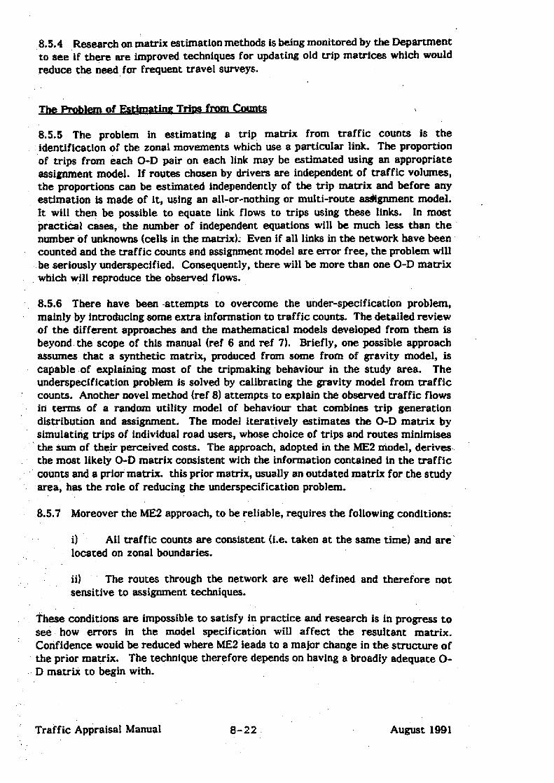
8.5.4 Research on matrix estimation methods is being monitored by the Department t o see ff there are improved techniques for updating old trip matrices which would d u c e the need for frequent travel surveys.

8.5.5 The problem in estimating a trip matrix from traffic counts is the identification of the zonal movments which use a particular link. The proportion of trips from each 0-D pair on each link may be estimated using an appropriate assignment model. If route chosen by drivers are independent of traffic volumes, the proportions can be estimated independently of the trip matrix and before any estimation is made of it, using an all-or-nothing or multi-route dgnment model. I t will then be possible to equate link flows to trips using these links. In most practical cases, the number of independent equations will be much less than the number of unknowns (cells in the matrix). Even if all Iinks in the network have been counted and the traffic counts and assignment model are error free, the problem will be seriously underspecified. Consequently, there will be more than one 0-D matrix which will reproduce the 0-4 flows.

8.5.6 There have been attempts tu overcome the under-specification problem, mainly by introducing some extra information to traffic counts. The detailed review of the different approaches and the mathematical models developed from them is beyond the scope of this manual (ref 6 and ref 7). Briefly, one possible approach assumes that 8 synthetic matrix, produced from some from of gravity model, is capable of explaining most of the tripmaking behaviour in the study area. The underspecification problem is salved by calibrating the gravity madel from traffic counts. Another novel method (ref 8) attempts to explain the observed traffic flows in terms of a random utility model of behaviour that combines trip generation distrfbution and assignment. The model Iteratively estimates the 0-D matrix by simulating trips of individual road users, whose choice of trips and routes minimises the sum of their perceived costs. The approach, adopted in the ME2 model, derives the most likely O-D matrix consistent with the infomation contained in the traffic counts and 8 prior matrix. this prior matrix, usually an outdated matrix for the study area, has the role of reducing the underspecification problem.

8.5.7 Moreover the ME2 approach, to be reliable, requires the following conditions:

i) located on zonal boundaries.

All traffic counts are consistent (i.e. taken at the sane time) and are

ii) sensitive to assignment techniques.

The routes through the network are well defined and therefore not

These conditions are impossible to satisfy in practice and research is in progress to see bow mors in the model specifiation wiIl affect the resultant matrix. Confidence wouid be reduced where ME2 leads to a major change in the structure of the prior matrix. The technique therefore depends on having 8 broadly adequate 0- D matrix to begin with.

’ Traffic Appraisal Manual 8-22 August 1991

8.5.8 The ME2 model estimates s matrix which is 8s close as possible to the prior matrix but reproduces the traffic counts when loaded onto the network. Closeness may be defined in tsrms of either absolute numbers of trips between each 0-D pair or prupurtiuns of total trlps that take p k e between each U-D pair, If there are no significant changes in travel patterns over the perhd of updating of the prior matrix, the two approaches will produce similar results. Otherwise, the resulting estimated matrices w€lI be different.

8.5.9 The matrix is estimated iteratively, whtch works typically as follows:

i) technique.

Tbprior matrix is assigned to the road network using an appropriate

ii) with the traffic count figure and an updating factor is calculated.

For the first traffic count the assigned flow on the link €s compared

iii) Thfs factor is applied to each 'relevant' cell in the prior matrix. A cell is relevant only if trips between the origin and destination zones use the counted link under consideration.

iv) factor based on the second traffic count is calculated,

The modified matrfx is then assignEd to the network and the updating

The procedure is followed for each traffic count in turn and repeated until the flows on all links in the network are in close agreement with the observed values.

8.5.10 At present, there is insufficient experience on the use of a ME2 model to provide advice on how to obtain 8n acceptablehse year trip matrix as a matter of routine.

8.5.1 I The basic requirements, given here, should only provide the conditions necessary to estimate a trip matrix which when loaded onto the network reproduces the observed link flows to 8 reasonable degree of accuracy, The acceptability of a base year trip matrix must depend on the outcome of checks of 0-D movements against independent obsewations. The basic requiremen= of the Matrix Estimation Technique are:-

i) The prior matrix should be obtained, in the main, from obseryed trip data. The matrix should reflect a pattern of tripmaking broadly similar to that implidt in the current traffic counts for the entire study area.

.

ii) of junction tuyning movements at critical intersections.

A good network definition should be used, which may include definition


ffi) The mute choice mode& used to esdmate the proportions of trip usfng each Iink, should be the most appropriate tu the study &re& conditions. This might be estabiished by checkfng the estimated proportions against observed f hWS.

iv) The number of independent traffk counts, following corrections for normal f b w continuity conditions (flows into a node equals flows out of the node), should be at least equal to the number of zones in the study area. If a good prim matrix is available, fewer counts might be sufficient. The counts should be spread throughout the network, covering links close to zone boundaries and highest trafficked links especially. While link fIows should be the bash of the input data, the input and rriodelling of junction turning counts at critically intersections will ensure a better C8libr8tiOn.

8.5.12 All indirect methods of producing up-to-date trip matrices, inchding the ME2 technique, are prune to model specification errors. Matrices 50 produced should not be accepted for forecasting purposes without some' form of validation (see section 11-41. Research to date has not demonstrated that an ME2 estimated mstrix reproduces the observed matrix more accurately than B matrix obtained by the alternadve growth factoring technique. Although both techniques may produce simflar results, the validation of a traffic model based on an estfrnated matrix could be different from the one based on a growth factored matrix.

8.5,13 The ME2 model is constrained to reproduce observed flow on selected links and these flows cannot be used for psignment model validution purposes. To validate the assigned traffic fiows, the model output should be compared witb count infomation resewed from that assembled for the matrix esth8tion. For a model based on 3 growth factored matrix (eg estimated growth in trip ends), the assembled count information shuuld be sufficient for assignment model validation purposes (see f 1.41-


8.6. I Disaggreg8dm is the process of breaking down output from 8 modd caifbrsted at one level of zone size to relate to zones of a smalier she. In this section, the term "parent zoned' is adopted to desaibe the large zones from the original system, with zonesw for the smaller zones, on the understanding that disaggregation will only he carried out Iocaliy for scheme evaluation ptnposes.

8.6.2 The tupics covered in detail in this section me:-

i) dkaggregathg land use planning data;

ii) disaggregsting the national car ownership made1 output;

iiil disaggregating the national private vehicle trip end model output; and

iv) disaggregating tr€p matrices,

8.6.3 Before becoming entangled in the details of disaggregating particular mode1 outputs, it is worth considering the techniques available for dhggregation fa general. The technique used will depend upon the form of the model. Models which are household or person-based will be almost independent of the zoning system for which they were developed and model output can be disaggregated shp ly by r e - m n g the model with input at the scheme zone level. However, models which rely upon zonal characteristics for the cdibratfon of model parameters cannot m a r i l y be -8ted In this way and other means must be found.

8.6.4 One general point cuncernfng dissggmgatfon, at aI1 times the aim is to redistribute the output from the parent zone which w€lI be assumed as a control total,

8.6.5 For estimates of land use planning data a t scheme zone level it will be necessary to go back tu the original SOUTCES (see section 4.5) and it is important tu remember that all estimates of I8nd use planning data are fnherently uncertain. When developing data for scheme zones ft Is to be expected that different sppmaches tu the problem will yieid different answers and one is left with the problem of deciding which of two or more estimates is the more valid. As always the solution is to test the sensitivity of model output t o see whether the differences are significant. NomalIy, because of the control to parent zone data, dffferences will not be great and c8n be ignored: if they are, and Cannot be resalved fn discussion with the Local Authority, the sensitivity tests ~ € 1 1 be iooked at to determine the effects of the uncertainty.

Trafffc Appraisal Manus1 8-25 August ,1991

8.6.6 The national car ownership model is essentially a household based model. Zone dependent facturs are included, however, in the form of the mean zonal income and the model is banded into six ieveL of urbanisation for which model parameters 8re independently estimated. A full description of the mode1 is given in sectfun 7.2.

8.6.7 Scheme zone data can be produced from this model by running the model at scheme zone level using the mean local zonal income and the level of urbanisatfon factors appropriate tu the parent (in the case hcaI) zone. However, if there are more than 10 or so scheme zones in a local zone, then the mean zonal income for each scheme zone should be estimated from census data. This process is not straightforward, being derived from car ownership estimates in the census and the inverse car ownership to income relationship, The level of urbanisation is a come factor whkh will not vary for any scheme zone in a local zone. Details of how tu run the model at acheme zone level, and advice on how to estimate rhe mean 20x181 income from census data, are available from EEA division.

Disaggremt inn the National Private Vehicle T r i ~ End M o d d c h r w

8.6.8 For the purposes of dissggregating model output, the nation81 private vehicle trip end modeh can be spIit into two categories:-

1) household-based models; and

ii) zuna1-based models.

Further details of these models are to be found in section 7.3.

8.6.9 The home-based work, home-based employer's business and home-based-other trip generation models are all household-based models which are banded only by zone type. Scheme zone data can be produced directly from these modeh by running the model with scheme zone input data using the model. band appropriate to the parent fIocaI1 zone.

8.6.10 The non-home-based trip creation model, the non-home-based trip alIocation model snd the home-based trip atvactian models are all zonal-based mode15 calibrated by regressing zonal trip ends agsinst zonal characteristics. Thk means that the calibrated model parmeten may be related to the size of zone fur which they were estimated snd I t cannot be assumed that these parameters wfIl be appropriate to any other zone site.

8.6.1 1 When using trip end models i t must be remembered that trip attractions are balanced to trip generations over specified areas. This makes it doubly important to control trfp ends at the scheme zone level to the parent zone totals to ensure the adoption of the sppropriate scaling factor for the trip attractions.

Traffic Appraisal Manual 8-26 August I99 1

FIG. 8.2

Matrix disaggregation by simple mathematical proportioning

'

0

3nslder a 3 r o n e t r i p matrix of which one zone ( A ) IS to b e disaggregated into 3 zone

15 1 21 I 24 90 30

3 0 0 ~ 3001 3 0 0 a 4 0 0 ~ SO- 0 . 2 5 ~ 0 . 3 5 ~ 0 . 4 ~ 1 . 0 ~ 1 - 0 s

AY : 0 . 4 ; AZ = 0.3.

It

Attractions AX : 0 . 2 5 : AY 0.35: A 2 8 0.4.

Original trip matrix

I600 5750 5300 Z1650

AX AY A L B C

P I ?.Ox( 1.031 r . o x l 1 . o x l 1.011

Disaggregated trip matrix

1 f

S 180

Z 240

I180

5 730

I f600


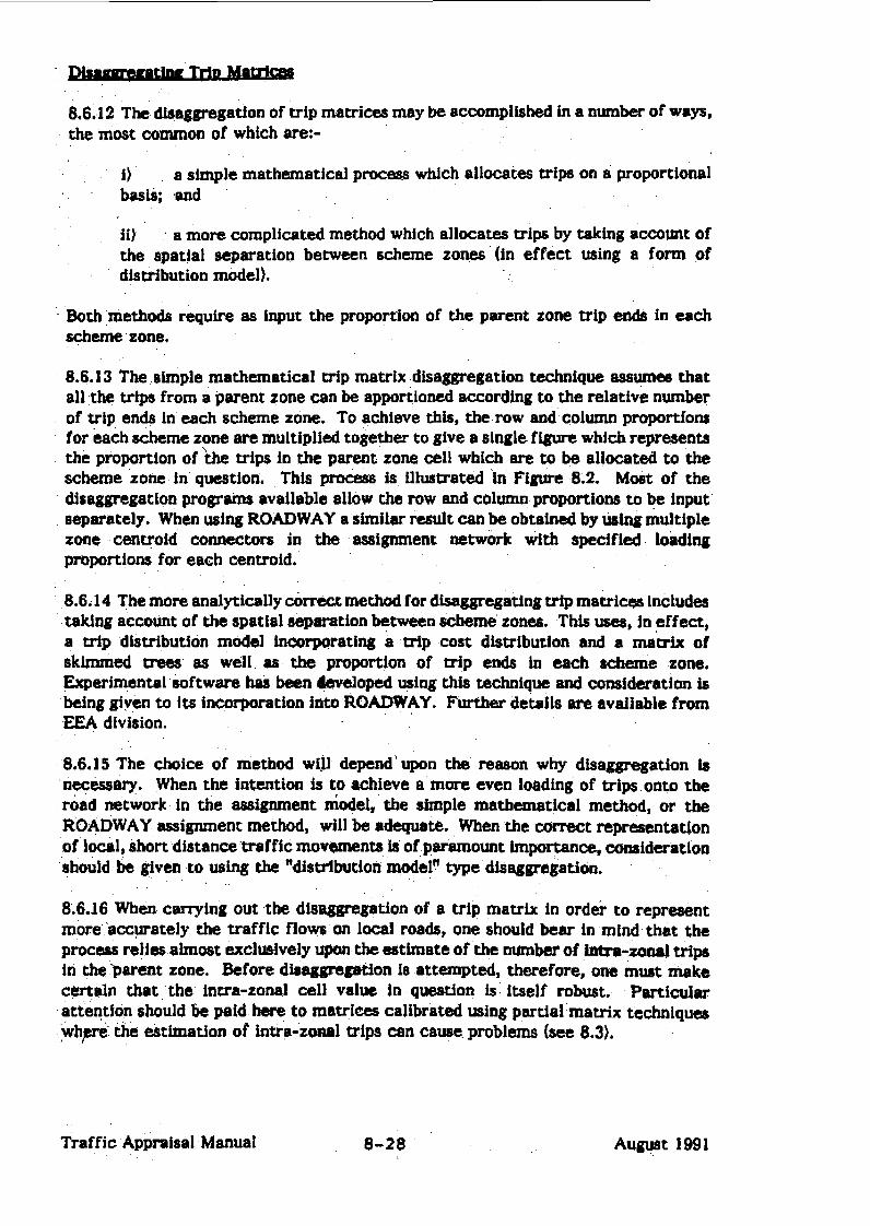
8,6,12 The ctbaggregatfon of trip matrim may be accomplished in a n u m b of ways, the most common of which are:-

I ) bash; and

a simple mathematical process which aIIocates trfps on a proportional

ii) a more complicated methud which allocates trips by taking account of the spatial separation between scheme zones (in effect using a form of distribution model).

Both methods require as input the proportion of the parent zone trip ends in each scheme zone.

8.6.13 The a h p l e mathematical trip maWx disaggregation technique assumw that all the trips from a parent zone can be apportioned according to the relatfve number of trip ends in each scheme zone. To achfeve this, the row and column proportfons for each scheme zone are multiplied together to give a single figure which represents the proportion of 'the trips in the parent zone cell which are to be aIIocated to the scheme zone fn question. This procerr~ is fliustrated in Figure 8.2. Mwt of the disaggtegatfon program available 8How the row and column proportions to be input sepatately. When using ROADWAY a similar result c m be obtained by using multiple zone mtrofd c o ~ e c t o m in the assignment network w€th specified loading pruprttons for each centroid.

8.6.14 The more analytically comkt method for disaggregating trip maul- includes taking account of the spatial separation betweun scheme zones. This USES, in effect, a trip distribution model InCorporatfng a trip cost dismbution and a mawix of skimmed treehi as we11 as the proportion of trip ends in each scheme zone. Experimental software han been &veloped wing this technique and considcretfon being given to iu incwporation into ROADWAY. Futthr detalls are avriiable from EEA division.

8.6.15 The choice of method will depend'upon the reason why disaggregation is neceamy. When the intention is to achieve a more wen loading of trips onto the road network In the Sssignment mod& the simple mathem~tlcal method, or the ROADWAY assignment method, will be adequate-. When the correct reprmentation of local, short distance traffic movements k of p&ramount importance, amideration should be given M uslng the "distribution mod@ type disagjpgation.

8.6.16 When carrying out the dimaggregation of a trip matrfx in order to r e p r a t more accurately the traffic flows on local roads, one should bear in mfnd that the process relies a h m t exclusively upan the %stImate of the "bw of m-zaad trips in the Parent zone. Before disagpgstion is attempted, therefore, one must make certain that the intra-zonal cell value in question is itself robust. Parciaiar attentlon should be paid hure to matrices calibrated using partial matrix techniques whpe the estimation of intra-zoml trips can cause problems (see 8.3).

Traffic Apprrrisal ManuaI 8-28 August I991

Fur these reasons it is not recumended that the national commescial vehicb trip matrices are disaggregated for use fn scheme appraisaI wfthout a thorough varidation of the resulting trip matrices.

8.6.17 Trip matrices formed from ubsented data can be created at a finer zoning level by going back to the original trip records and the problem should usually be approached in this way. However, disaggregation may be appropriate either when the survey records are suspect or when the problem is simply one of giving a more even loading of trips on to the road netwurk in the assignment model.

Traffic Appraisal Manual 8-29 August I991

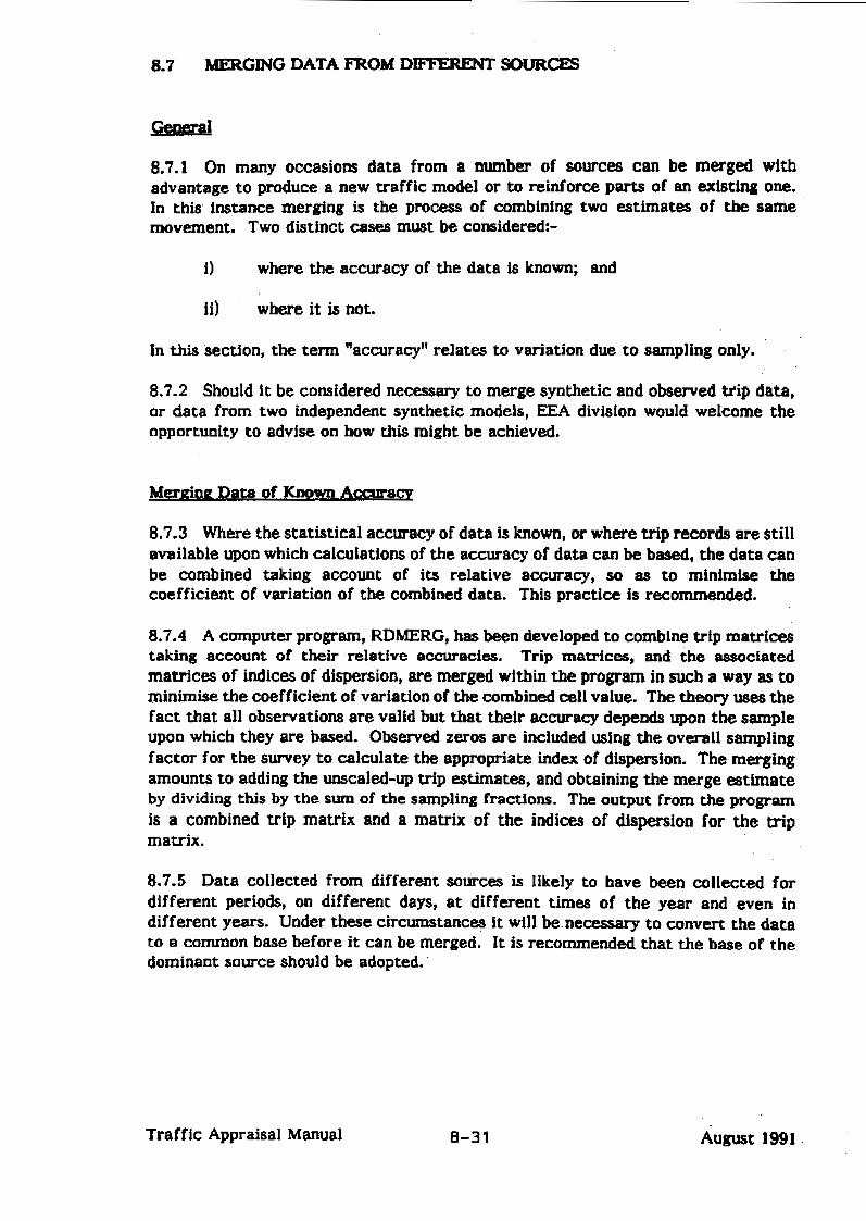
8.7 MERGING DATA FROM DIFFERENT SOURCES

8.7.1 On many occasions data from a number of suurces can be merged with advantage to produce a new traffic model or to reinforce parts of an existing one. in this’ instance merging is the process of combining two estimates of the same movement. Two distinct c a w must be considered:-

i) where the accuracy of the data is known; and

ii) where it is not.

In this section, the term “accuracy” relates to variation due to sampling only.

8.72 Should it be considered necess- to merge synthetic and observed trip data, or data from two independent synthetic models, EEA division would welcome the opportunity to advise on how this might be achieved.

8.7.3 Whwc the statistical accuraq of data is known, or where trip records are still available upon which calculations of the accuracy of data can be based, the data can be combined taking account of its relative accuracy, so as to mIn€mise the coefficient of variation of the combined data. This practice is recommended.

8.7.4 A computer program, RDMERG, has been developed to combine trip matrices taking account of their relative accuracies. Trip matrices, and the assodated matrices of indices of dispersion, are merged within the program In such a wry as to minimise the coefficient of variation of the combined cell value. The theory uses the fact that all observations are valid but that their accuracy depends upon the sample upon which they are based. Observed zeros are included using the overall sampling factor for the surrey to calculate the appropriate index of dispersion. The merging amounts to adding the unsealed-up trip estimates, and obtaining the merge estimate by dividing this by the sum of the sampling fractions, The output from the program is a combined trip matrix and a matrix of the indices of dispersion for the trip matrix.

8.7.5 Data collected from different sources is likely to have been collected for different periods, on different days, at different times of the year and even in different years. Under these circumstances it will be necessary to convert the data to a common base before it can be merged. I t is recommended that the base of the dominant source should be adopted. ’


8.7.6 The merging of data from different sources when the relative accuracy of the data is not known statistically will depend upon the information available to the traffic engineer. When possible, an estimate of the relative accuracies of the trip matrices should be made wing the average scaling-up factor for the observed cells in each survey. The average scaling-up factor for a survey is the estimated number of trips crossing an interview cordon divided by the number of intemiews sccumpIished. The relative accuracies can be estimated and the data merged giving greater weight to the more accurate data.

8.7.7 When even rudimentary information on the sampling framework of the srvreys is not available, the traffic engineer must use his judgement to decfde how to use the data. The options are:-

i) number of trips recorded in the surveys;

where the surveys are considered to be of equal merit, to average the

i i ) data from this survey in preference to the others; and

when one survey is considered to be better than the others, select the

iii) weights).

to merge giving greater weights to one than another (eg 2 to 1

Person81 knowledge of one survey is a valid factor and shouid be aIlowed to influence the decision.

Traffic Appraisal Manual 0-32 August I991

8.8.1 Matrix manipulation is primarily a mechanical process. exercised to ensure that matrix operations are valid and necessary.

Care should be

8.8.2 Matrix manipulation is necessary to convert gravity trip distribution model output from generation 8nd attraction (G-A) format to the origin and destination (0- D) fonnat required for assignment. The pracfss assumes that of the trips generated by a household, half will be made away from the home end, and half towards it. The G-A matrix will& subjected to the following operations:-

i) transpose the E A trip matrix to give matrix Z;

ii) add matrix 2 to the G-A matrix to give matrix Y; and

iii) divide &mix Y by 2 to give the 0-D trip matrix required.

8.8.3 The ROADWAY program RDMAT includes routines to cmy out the above, and many other, matrix manipulations, AddMonally, RDMERG should be used to add together trip matrices when the acctrracy of the cell estimates due to sampling theory is known. This will be appropriate when trip matrices for individual trip purpose and vehicle types are combined prior to assignment, RDMERG outputa a summated trip matrix and a matrJx of the indices of dispemion for the combined trip matrix.


Tref f ic Appraisal Manual 8-34 August 1991

1. Phillips G (LGORU): "Accuracy of annual traffic flow estimates from short period counts", TRRL Supplementary Report 514.

2. Phillips G (LGURU): 'Accuracy of annual traffic flow estfmates from automatic costs", TRRL Supplementary Report 515.

3. Day M J L and Hawkins A F: "Partfa1 matrices, empir€cal deterrence functions and ill-defined results", Traffic Engineerfng and Control, AugustISeptember 1979, p429-433.

4. Gunn H F, Kirby H R, MurchIand J D and Whittaker J C: "RHTM: Trip Distributfon Investigation?', The Instftute for Transport Studies UhIversfty of LeeddAlasmir Dick and Associates, May 1980.

5. "Forecasting Traffic on Trunk Roads: A Report on the Regional Highway Traffic Model Projectnf the Standing Advisory Committee on Trunk Road Assessment, HMSO, December 1979.

6. Van Zuylen H S and WiIlumsen L G: 'The most likely trip matrix esthated from traffic counts", Transpn Res B. Vu1 14B pp 281-293, Pergamon Press Ltd. 1980.

7, WiIhuxnsen L G: "ShpIified tansport models based on traffic counts"; Transportat€un 10 (1981) pp 257-278; EIservier Scientffic Pubhhfng CO, Amsterdam.

8. Robertson D I: Tstimating or€gin-destination flows by simulatfng trip choice"; Traffic Enjgineering & CuntroI, July 1984.

9. SACTRA P(82114: The Development, Calibration and Validation of the National Model of Long Distance Traffic: Unpublished)

10. "RHTM: Project Review"; Alastak Dick 8d Associates, September 1978.

11. "RHTM: Development of Private Vehicle Base Year Matrices based upon the Hybrid Approachw; Ahstair Dick and Associates, September 1978.

12. T€HTM: Private Vehicle Base Year M 8 t r i W ; Calibration and Validstion Comparisons, February-May 1979" ; Alastair Dick and Associates, 1 June 1979.

13. ?RHTM: Private Vehide Base Year Matrices; Calibration and VaIidadon Comparisons, August-October 1979"; Alasteir Dick and Assodates. 31 October 1919

Traffic ApprsiSaI Manu81 8-35 August 1991

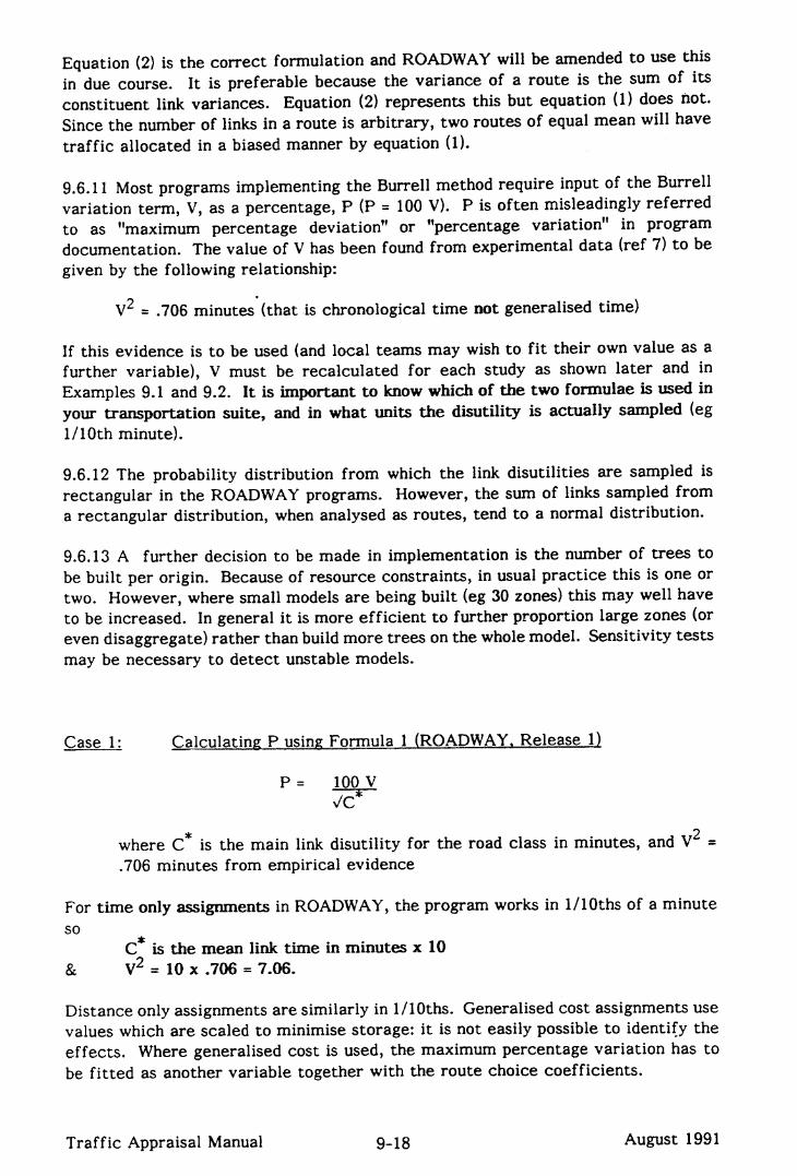
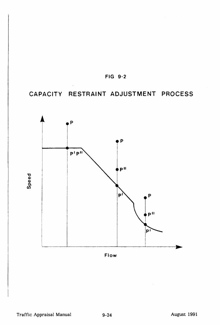
k

CHAETER 10 : THE ASSESSMENT OF ERRORS IN THE BASE YEAR

10.1 INTRODUCTION

10.2 ERRORS

10.3 ESTIMATING THE ACCURACY OF GROUND COUNTS

10.4 ESTIMATING THE ACCURACY OF TRIP MATRICES

10.5 ESTIMATING THE ACCURACY OF ASSIGNMENTS

10.6 USING THE BASE YEAR ERROR ESTIMATES

10.7 USING ACCURACY ESTIMATES IN MODEL DESIGN

REFERENCES- CHAPTER 10

Traf fit Appraisal Manual August 1991

C!HlWER 10 : THE ASSESSMENT OF ERRORS

IN THE BASE YEAR

10.1 INTRODUCTION

10.1 .l The results obtained from all traffic appraisals are uncertain. That is not to say that we do not know what the results are! Rather that any set of results is produced using a combination of input forecasts and modelling assumptions for which alternative values could have been substituted to give another set of values which might be equally valid. The total uncertainty of an estimate resulting from the use of a traffic model is a combination of the statistical errors of measurement and sampling, the specification errors of the mathematical models used, and the errors implicit in forecasting. It is essential that the uncertainty in model output is recognised, and quantified as far as possible, so that due allowance can be made for it when decisions are taken.

10.12 The treatment of uncertainty adopted in this manual is in two stages. There are recognised statistical methods of assessing errors in the base year which is the subject of this chapter: these lead to an improved understanding of the quality of the information produced by a traffic appraisal. Uncertainty in forecasting is not capable of assessment in the same way, and while research is continuing in this area the emphasis is rather on how to take account of it in decision making. The approach to be adopted when forecasting traffic flows on trunk roads is set out in Chapter 12.

10.1.3 This chapter initially explores the nature of the “errors” implicit in traffic models, and the way in which allowance for these errors can be made. Further sections cover the use of the accuracy estimates produced and the way in which the lessons learned can be fed back into the system to improve the cost effectiveness of the models.


10.2 ERRORS

General

10.2.1 Attempts to quantify uncertainty involve the concept of error. The word error, in this context, is used in its classical statistical sense: it does not mean a blunder or mistake (although these will always occur when human beings are involved in data collection and processing, and are also discussed here), but refers to the differences which arise from alternative measurements of a quantity using different measuring techniques or samples.

10.2.2 When dealing with traffic models, these errors, may be grouped under three headings:-

i) data errors;

ii) model specification errors; and

iii) forecasting errors.

Statistical techniques can be used to minimise the first during model fitting and to estimate the second. Forecasting errors will not be further discussed here, but in chapter 12.

Data Errors

10.2.3 Data errors are concerned with:-

i) errors due to sampling;

ii) measurement errors; and

iii) blunders.

Sarmlinn errors

10.2.4 Sampling is the process of drawing a representative set from a population with the intention of using the characteristics of this set to describe the population as a whole. Sampling error is the variation in the estimation of the characteristics of the whole population which could arise from measurements based upon one or more samples drawn independently from the population. The variation due to sampling can be estimated if reasonable assumptions are made about the way in which the sample is drawn.

Traffic Appraisal Manual 1 o-3 August 1991

10.25 Sampling errors arise in traffic appraisals because most of the data upon which the models are based is sampled data. A roadside interview will embrace only a

proportion of the traffic during the survey period: household interviews usually cover only a small percentage of the total households in an area: both methods sample trips for a limited period, perhaps only one day, and this is taken as being representative of a longer period.

Measurement errors

10.26 Measurement errors can arise from using different methods of measurement to quantify a parameter. For example, network links may be measured precisely using a horizontal alignment program, or scaled from maps: land use planning data for small areas can also vary greatly between national estimates and those produced locally, sub-divisions of employment data are particularly sensitive. Measurement errors can also occur due to the adoption of definitions which can be ambiguously interpreted resulting in data being mis-classified. Definitions have proved difficult to interpret in interviews: for example, asking a driver to discriminate between a journey to work and a journey carried out on his employer’s business can cause problems. Allocating the correct purpose to “serve passenger” trips, such as taking one’s children to school whilst on one’s way to work or “kiss and ride” trips, can also cause problems.

Blunders

10.2.7 No matter how many coding and data checks are carried out, pure blunders will still arise in any data which has been collected from and by human beings. A comprehensive set of data checks will minimise these, however. A further check when fitting a model is to examine the outliers (extreme values) in the residual model errors to ensure that the data are valid. Any blunders which do not appear as extreme values are unlikely to significantly affect the model calibration.

Model specification errors

10.2.8 Model specification error can be defined as the difference between the true value of a dependent variable tie, a perfect measurement without error) and the model prediction of the value. Such errors arise when a mathematical model is not a perfect representation of the true situation.

10.2.9 All the mathematical models used in traffic modelling are attempting to represent human behaviour. it is axiomatic that such models can only approximate behaviour and will, therefore, be subject to specification errors. It is possible to specify very complex models in an attempt to take into account the many variables which in reality influence travel behaviour. But these models would probably be of limited value in forecasting - the inputs being as difficult to forecast as the final result.


In practice, therefore, the variables included in a traffic model are chosen as those which it is sensible to assume do influence why people buy a car, choose a destination, select a route and so on; and which can be forecast with a reasonable degree of confidence.

10.2.10 Model specification error is inherently difficult to quantify. The errors may be revealed in a poorly fitted base year model, but more often the errors become apparent through time, the chosen variable ceasing to be strongly correlated with the true causal variables. As all the available data is commonly used to decide upon the model specification and to calibrate the parameters of the chosen model, only comparison with independent data during model validation or monitoring the performance of the model through time can reveal model specification errors.

10.2.11 One interesting case of specification error has recently come to light with the “Disaggregate Model of Household Car Ownership” developed by Bates, Gunn and Roberts which was published as DoE/DTp Research Report 20 (ref 1). The model was calibrated to data from the Family Expenditure Survey for the period 1965-1975 and used household income relative to car prices to predict household car ownership. This was a rigorous piece of research and the resulting model appeared to be well specified in that the unexplained variation in the data was negligible. The error in model specification appeared in respect of data for the period 1976 to 1978. During this period car prices rose in real terms whilst real gross household income rose to a much lesser extent; a combination of circumstances which were not experienced between 1965 and 1975 and which, according to the model, should cause a fall in car ownership. in fact car ownership has continued to increase. There are many plausible explanations for the continued increase in car ownership which are not relevant here, suffice it to say that on the basis of the data available up to 1975 the model appeared well specified, but since that time circumstances have changed and the model specification now appears less satisfactory. The model has been amended subsequently and SACTRA has commented upon its use in producing national forecasts (ref SACTRA - National Traffic Forecasts - March 1980 (Unpublished)).

10.2.12 When fitting a model, the best guide to the adequacy of the model specification in the year of calibration are the residual errors, that is the difference between the observed and modelled values. General advice on what to look for when fitting models would include the following points:-

i) examine the independent variables and judge whether the apparent relationships to the dependent variable are meaningful with a “causal” foundation and not coincidental;

ii) ensure that the independent variables are easier to forecast than the dependent variable;

iii) when choosing between highly correlated independent variables, only one of which should be included in the model, ensure that the variable included is that which is most likely to explain changes over time and for which future values can more easily be forecast; and

Traffic Appraisal Manual 1 o-s August 199 1

iv) examine the residual errors thoroughly, including by plotting, to ensure that the residual errors are normally distributed and do not display any bias.

102.13 These then are the various types of error with which we are concerned in the base year. The following sections consider how the errors affect the data collected, models fitted to that data, and the interpretation of the results produced by the models.

Traffic Appraisal Manual 1 O-6 August 1991

10.3 ESTMATING THE ACCURACY OF GROUND COUNTS

10.3.1 Ground counts are :-

i) counts carried out by automatic traffic counters (ATCS); and

ii) classified counts by both manual and automatic means.

These basic methods count the traffic passing a point on a road. They are different in terms of the data collected, the method of collection, and the assessment of the likely errors.

Automatic traffic counters

10.3.2 Little definitive work has been published concerning the accuracy of traffic counts by automatic traffic counters. Experience suggests that the errors are machine and (particularly) installation dependent. For longer term counts, the frequency and diligence of the station monitoring and servicing will be crucial.

10.3.3 Intrinsically, inductance loop detection should be more reliable than pneumatic tube detection. However, to obtain high quality results with loop detectors on multi- lane sites it is essential that the loop installation is of the highest quality and the electronic detection equipment correctly adjusted. This generally implies the use of a frequency meter. The major drawback with pneumatic tube detection, now that high quality electronic air switches are available, is that they count the number axles (or pairs of axles) rather than the number of vehicles which is the required quantity. A factor must then be applied to convert to the number of vehicles that went by, an additional source of error over and above the “mechanical” error of the counting apparatus itself.

10.3.4 Using the limited information available, the current best “working” estimate of the accuracy of measurement of the number of vehicles that passed an automatic traffic counter is that the 95% confidence interval of a count of longer than 12 hours duration is of the order of f 5% of the total count (Before and After studies: Stage II report - ref 2). This assumes that the counter was installed and maintained to the standards laid down in the “Manual of Automatic Traffic Counting Practice” (ref 3). Recent work by the GLC supports this assertion (GLC TSN 232: Blackfriars Bridge Road Traffic Counters Experiment: May 1980 - ref 4). While counting for longer periods will yield more data, and will help to reduce the impact of human blunders and mechanical errors, it is unlikely that confidence intervals can be much reduced. This is because the data are correlated with the same counting equipment being used on the same site on contiguous days, and independent data are required to substantially increase reliability. For a counter using a pneumatic tube detector, the vehicle to axle ratio should be estimated from a manual classified count with the ratio assumed to be as accurate as the count from which it is derived.


10.3.5 When a short term automatic count is used to predict the average traffic flow for a longer period than the counter was on station, the estimated traffic flow will be subject to sampling error. The Local Government Operational Research Unit

(LGORU) has researched these errors on behalf of TRRL. Their findings are reported in TRRL Supplementary Report 515 “Accuracy of annual traffic flow estimates from automatic counts” (ref 5). This aspect of sampling error is more fully covered in section 6.2.

Classified Counts

10.3.6 Classified counts have traditionally been carried out manually, but an automatic classifier has been developed by TRRL. A statistical study of the reliability of manual classified counts (MCCs) has been carried out in DTp which is reported in a paper entitled “Checks on the Accuracy of Manual Road Traffic Counts, August 1979” (ref 6). The study consisted of an analysis of parallel counts recorded simultaneously by separate local authority and DTp teams at 13 of the 200 point census sites. The counts were subject to both counting error and vehicle classification error. The conclusion reached was “the true 16 hour flow of all motor vehicles at a given site lies, with 95% confidence, within an interval of about f 10% of the Local Authority count. The intervals for separate classes, except probably cars and taxis, would be wider than this.” The figure of f 10% is based upon the assumption that the variance of the DTp counts, taken by a dedicated experienced team, was half that of the LA counts. The 95% confidence intervals for some individual vehicles classes were:-

All Vehicles and Cars and taxis f 10%

Light Goods Vehicles + 24%

Other Goods Vehicles + 28%

All (light plus other) Goods Vehicles f 18%

The relatively wider confidence intervals for individual Goods Vehicle classes results largely from mis-classification between them, the accuracy of the total number of Goods Vehicles will be better than for an individual class. The intervals for individual hours are likely to be larger but the 16 hour figures can be taken as a guide. These results are reinforced by the GLC study mentioned in 10.3.4.

10.3.7 The eventual intention is that the core census count sites in the national census will be converted to use automatic classifying equipment when available. Production of this equipment in commercial quantities is still some way ahead and a complete assessment of the accuracy and reliability of both counting and classification will have taken place by then. It seems likely that this equipment will be fairly expensive and will demand a high initial investment at each monitoring site, rendering it suitable only where long term classified data is essential.


10.3.8 Once again sampling errors will come into play when a one day classified count is used to predict the average traffic flow over a longer time period. LGORU has also researched this problem, again on behalf of TRRL, as reported in TRRL Supplementary Report 514 “Accuracy of annual traffic flow estimates from short --T.;rrB-I -n.,ntr” (ref 71 yw IV&I b”UIAW which ic flrrther riicrr~rc~Tj in cprtinn 6,3, I ,, “AA&b.& .U l “I %...“a YlYYYYYYY 1.. “___-.e--

10.3.9 To assist in the application of the errors arising from ground counts, EEA division has developed general purpose computer software (RDCVAR) to process count data to yield the coefficient of variation of any estimate (say AADT) made from 12 or 16 hour counts on any day. The software, written in portable Fortran to HC specifications is available for use on mini and micro computer installations.

k


10.4 ESTIMATING THE ACCURACY OF TFUF’ MATRICES

10.4.1 When estimating the accuracy of trip matrices, there are different sources of error associated with:-

ij trip matrices formed directiy from expanded observations; and

ii) trip matrices output by a gravity trip distribution model.

Observed data triD matrices

10.4.2 Once the appropriate data checks have been carried out, trip matrices formed directly from expanded observations will be subject to errors due mainly to the use of sampled data. RDMVAR is a matrix building program which has been developed for addition to the ROADWAY suite. The program estimates the variance of each observed cell due to sampling and outputs a matrix of the index of dispersion for each -L------l --.I observea ceil. * _.__ L__ _c __& __---C_--LLI_ ^^^ _._^ c:-,- L __._ e.. L., . . . .._..l~.L A IlUIIlDer 01 IlOL-UIII-edSOIldUlt: kiSSUIlll)L1U113 IlilVC

a finite

A single a number

hnttxrman nhctanmwl t-nllr urnnrltl nnd +n he r~lp~~latd (if nnccihlp) and . aA IOllbW Y~LW~c.~, ““OCII .bU UUII.? ““USU “bL.U C” “U “U*“Y.YCYY \a. y”YY’Y’v, V-I-

allowed for in each calculation. This simplification seems most likely to underestimate the variance of each cell by an amount dependent upon the correlation between cells;

iii) the data are assumed to be hierarchical in nature in the calculation of individual cell variances. This is a flexible assumption which allows the data to be properly d~cribed. The talc-elation allows a factor -~hlch affects large

amounts of data to be applied in such a way that the variance of the cells affected will be higher than when applied at a lower level. This will tend to offset the underestimation due to ii); and

iv) when estimating the index of dispersion for observed cells which are zero by chance, an overall grossing up factor for the whole screenline or cordon is adopted.

The precise effects of these assumptions will be fully investigated during the program testing and demonstration phases which are due to be completed in the ROs early in 1981.


TriD matrices from pravitv models

10.4.3 Trip matrices output by gravity trip distribution models will contain both specification errors and errors in the fitted parameters due to fitting to sampled data. Two methods of estimating the errors due to fitting the model parameters to sampled data are available:-

i) multiple fitting of the model using a Monte Carlo simulation with alternative sampled data drawn from the reference model first fitted to the observed data. The parameters fitted by successive calibrations are stored and the coefficients of variation of the fitted parameters calculated. Individual cell variances can then be estimated from this data; and

ii) analytical methods which would give a direct estimate of the cell (or fitted parameter) variance due to sampling variation in the input data.

Monte Carlo simulation (i) has been incorporated into RDGRAV2 and can be used with any of the available fitting methods. Advice on the use of this technique is given in the documentation supporting the program. An analytical method (ii) has been derived from the partial matrix fitting method. This is known as “Whittakers Approximation” and the technique and its use in survey design is fully described in section 6.12.

Snecification error

10.4.4 Specification error in trip matrices produced by gravity trip distribution models is difficult to assess. As is generally the case, the approach is to minimise specification error in the base year by fitting the model using all the available data, and examining the residual errors (the difference between observed and modelled cell values) as thoroughly as possible to ensure that the errors are random and normally distributed. A program called RDCOSM has been developed to calculate a number of statistics related to the residual errors to assist with these comparisons. Indicators of this type, based upon measures of difference, are experimental and experience of their use alongside existing criteria will be necessary before their usefulness can be assessed. RDCOSM is planned for release early in 1981.

10.4.5 When assessing the accuracy of trip matrices the purpose for which the trip matrix will be used is important and must be taken into account. The assessment will be concerned with whether the trip matrix is suitable for the intended use rather than if it might be classified overall as good or bad. In order to be acceptable for the intended use, a trip matrix must adequately reflect the traffic movements in the area of interest, or the corridor into which a scheme is to be inserted. For example, in the evaluation of a scheme in the Manchester to Birmingham corridor, the trips between Stafford and Stoke will be important but those from Stoke to Derby will have little influence upon the evaluation. All the software described in this section can be used to examine selected parts of a trip matrix: decisions on acceptability should be based upon the accuracy of the crucial parts of the trip matrix and upon validation criteria as described in chapter 11.


10.5 ESTIMATING THE ACCURACY OF ASSIGNMENTS

10.5.1 As the last model in the chain, the output of the assignment model is often more critically assessed than that of the other models. This is to be expected because it is the assignment model which produces the link flows by which the performance of the complete model will be judged, and the impact of highway proposals assessed.

10.5.2 The purpose of an assignment model in the base year is to predict link flows which are compatible with observed counts. To produce link flows the model fits representative routes through the network on the basis that travellers try to minimise some function of time, distance or weighted combination of the two. The real reasons why people choose a route are thought to vary greatly and are, to some extent, obscure: an assignment model will, therefore, contain specification errors. In addition, an assignment model will inherit the errors of the input trip matrix (see section 10.4) and road network.

_ ^ -. iO.5.S .l.he road network is subject to:-

i) measurement errors in the characteristics of the links included; and

ii) specification errors in the structure of the network, the selection of links and the number and location of zone centroid connectors (along which trips gain access to the network).

10.5.4 A measure of the variance of assigned link volumes due to sampling errors in the trip matrix can be obtained by loading a matrix of cell variances to the road network using the same trees as were used to load the trip matrix. Once again the assumption is that each cell is independent and, because correlations are ignored the -,el..,rl . ...11 as.1.. ,,,,,-*:-..b, a-L.1 ..-..:AW.-r. Ld........-- s.--,.:AI ..,.,C..l IlICLIIUU WI11 uu1y qJjJ1 UAlIllaLc Lilt: vu 1a11c;ts.

It .ai::, 11UW~VIsl) y1uv1uc: 8 U3lzll.u

indication of the accuracy obtainable. The steps involved are described in section 11.4.

10.5.5 Readers of previous sections will anticipate that the key to minimising model specification error in the year of calibration is the examination of residual errors (the difference between observed and modelled values). With assignment models it is recommended that a statistic of the Chi-squared form

{Observed - Modelled12 Modelled

is calculated and summed over a selection of links in the area of interest: the form of the model which yields the lowest value being adopted. Care must be taken when selecting the links to be included in ‘the calculation, particularly with observed data trip matrices, to ensure that all the trips likely to be assigned to a chosen link are included in the trip matrix. For this reason, the links which cross interview cordons or screenlines should be included. The fitting of assignment models is fully described in chapter 9.


10.6 USING THE BASE YEAR ERROR ESTIMATES

Introduction

10.6.1 The assessment of errors in the base year has two main applications:-

i) in model validation (chapter 11); and

ii) in the assessment of a model’s ability to discriminate between the traffic effects of alternative schemes.

The Assessment of a Model’s Ability to Discriminate

10.6.2 The traffic estimates which the traffic engineer produces from a study will form the basis for scheme assessment and will usually be used to test different options. When this is the case it would be helpful to determine whether differences in the traffic effects between alternatives are real and significant or whether they could have occurred by chance within the error structure of the model. Excluding forecasting error (which will be discussed in chapter 12), the two other sources of error (discussed in this chapter) are errors due to measurement and sampling, and model specification. In determining whether the traffic effects of alternatives are r:r....:C:~.-.“.e,.. rl:CC-,^,e IL, I?,-,- _^__ L- ^^^^^^^ 2 L-- -II___& ̂ ^LI_CL_ -_J ..L- ICLL__ 31~~llllLallLly UII 1 t21 CllL Lllt: 1 UI IllCZI lllklj’ Ut: LiSStZSStXJ LJJ’ UITtKL fZSL1IIldL.t: dIlU Lilt: IdLLtX-

by sensitivity testing. These techniques are discussed in this sub section.

Testinn whether Model OutDut is Simrificantly Different due to Measurement and SamDlinn Error

rn c 3 T, _--*:__ rn * ._~~l_-:-._-_ --- >-_-_lL_-l _..Lf-I_ _11_... AL- ---1---z-- -c -L- 1u.u.3 III S~LLIUII IV.*, ~ecnruques are aescx-meu wmcn allow rne esr;imai;lon or me

errors in the base year trip matrix due to measurement and sampling errors. Using this information, it may be possible to estimate the probability that the differences in assigned link flows predicted with alternative schemes are truly different. This is under investigation by EEA division, and further advice will be issued in due Pnl l?-CP “VU* “U.

Sensitivity Tests

10.6.4 Sensitivity tests may be considered in three categories:-

;\ emnll ~.-%,4...~L.~nc;~~r n+- CL._ -r...lP.l nrr-rrm-4-,.-- ..--A :- ---- -c AL_ ___I __=_‘l_ 11 5~~1411 yr;l LUI U~LIVIID UI LI~C I~IUUCI yai all1c~c13 u3eu III auy 01 Lue suD-moueIs

to ascertain the sensitivity of each sub model to the choice of parameter

value;

ii) selective sensitivity testing where the full feasible range of a parameter might be selected to ascertain the resulting range of a particular flows; and

Traffic Appraisal Manual 1 o-1 5 August 1991

iii) systematic sensitivity testing (ST). A structured approach to sensitivity testing which seeks to paint a picture of the likely range of outcomes by running a set of models with each parameter carefully chosen from a range.

Within the procedures recommended by this manual i) is used both in the base year and when forecasting, and is of particular relevance to the assignment model: ii) and iii) are used when forecasting and are covered in chapter 12.

10.6.5 To assist in determining whether the differing traffic effects of alternative schemes are not real and significant but due to specification and parameter errors it is necessary to ascertain the sensitivity of the output link flows to the choice of model form and the chosen model parameters. Tests of this kind are usually associated only with the assignment model where the fitting process is more difficult to control statistically than elsewhere: it is therefore recommended that small changes in the route choice parameters should be made (for example, a 10% change in the b/a ratio) and the assignment reproduced to assess model sensitivity. This process will draw upon the knowledge gained from fitting the assignment model in section 9.6. Judgement should then be used to assess the significance of differences in model output.

Traffic Appraisal Manual 1 O-l 6 August 1991

10.7 USING ACCURACY ESTIMATES IN MODEL DESIGN

10.7.1 A number of themes run through this manual with the common aim of achieving cost effective traffic appraisals. ‘FL- -^c-_ __^^ -c ^-^_--L-__ -I----2L--l I-..--

1 Ilt: Iilt5dSLKt!S 01 tlr;r;Ul-dCJJ’ UBCI-IUBU IIlLtX-

alia are the first comprehensive attempts to quantify the errors in traffic models used for trunk road appraisal: armed with these weapons it is possible to examine critically the performance of each model to define the contribution of the errors in each to the overall result. This section is concerned with the way in which the leccnnc tn hP learnd will he fd hark intn tho cvctem tn .W”“..” C” Y” A”“. ..“V ..A.. “U .“U “Y”‘. I.._” C..” “,“CY*** C”, ifi time nntimico tho C....“, “~C.*aI~U~ L,,b

balance between cost and accuracy of the modelling stream.

10.7.2 The learning process begins with the examination of the accuracy of the models currently in use to highlight where:

i) additional data collection will significantly improve the accuracy of the fitted model;

ii) little accuracy in the fitted model would be lost with significant reductions in data requirements;

iii) an existing model specification is inadequate suggesting that research into alternative model forms might be worthwhile.

Traffic modelling is a sequential process and the optimum combination would seem to be when all the models are equally accurate, since the least accurate tends to dominate the accuracy of the overall result. To illustrate this it is possible at a roadside interview station to interview all, or a very high proportion of, the vehicles which oass through the station on the survey day, Whilst this wil! give a high!y r ~~

accurate estimate of the observed trip matrix for that day (accuracy being dependent upon sampling rate), the estimate of 24 hour AADT obtained will be governed by the accuracy of the assignment model and the conversion factor used. A significant reduction in the number of interviews might have a small impact upon the final level of accuracy attained.

10.7.3 The “horses for courses” argument (the selection of the simplest form of model appropriate to the current appraisal) is also relevant here. Each model should be of a form chosen to achieve the specified objectives of the current appraisal and should provide a level of accuracy appropriate to the decision at hand. The lowest level of accuracy will be required for the feasibility study when all the information concerning the proposal will be highly inaccurate (eg construction costs): the usefulness of data from the fringes of existing models in use for other studies should not be overlooked here. The highest accuracy will be required to discriminate between the traffic effects of alternative schemes and for design purposes. It should be recognised that traffic models cannot be built on a once and for all basis: different levels of data are necessary as a scheme proceeds through the preparation process with more detail being added as time goes by, either by means of a new traffic study or by enhancing the existing one -..-- --._ o -__-: This will be particularly jmnnrtcint y”A CUIlL

when the preparation of a scheme has been interrupted.

IO-17 A.._- -1 .r\n. August lYY1

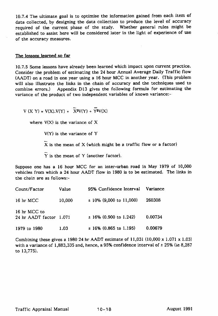
10.7.4 The ultimate goal is to optimise the information gained from each item of data collected, by designing the data collection to produce the level of accuracy required of the current phase of the study. Whether general rules might be

established to assist here will be considered later in the light of experience of use of the accuracy measures.

The lessons learned so far

10.7.5 Some lessons have already been learned which impact upon current practice. Consider the problem of estimating the 24 hour Annual Average Daily Traffic flow (AADT) on a road in one year using a 16 hour MCC in another year. (This problem will also illustrate the links in the chain of accuracy and the techniques used to combine errors.) Appendix D13 gives the following formula for estimating the variance of the product of two independent variables of known variance:-

v (X = V(X).V(Y) + XWY) + *v(x)

where is the variance X

Suppose has a MCC an

lo-18 August 1991

10.7.6 The MCC could have been made absolutely accurate (by video recording and multiple interpretation), but would a worthwhile increase in accuracy result? Using the above information with the variance of the MCC equal to zero gives an estimate of 11,031 + 23% (ie 8531 to 13531), hardly any increase in accuracy. This is because the accuracy of the estimated 1980 24 hr AADT traffic flow depends largely upon the accuracy of the 16 hr MCC to 24 hr AADT and the year to year factors, which are the most uncertain elements. The overall accuracy of the 24 hr AADT estimate is not surprising; in effect, the 16 hour count is being used to predict the traffic flow in a calendar year of 8,760 hours, a sampling rate of about 1 in 550.

10.7.7 This result has a number of implications for practical traffic modelling:-

i) the simple fact of collecting more (accurate) observations does not necessarily result in worthwhile increase in the accuracy of the final result;

ii) data should be factored as few times as possible to avoid the cumulative effect of uncertain factors, particularly prior to validation;

iii) where local factors are derived for use in specific studies, the accuracy of each factor should be calculated and taken into account in its use (the accuracy of a factor is dependent upon the number of observations from which it has been derived, and their variability); and

iv) in producing estimates of AADT for assessment purposes, the accuracy of the factors used is crucial: EEA will consider ways in which the accuracy of these factors might be improved.


REFERENCES- CHAPTER 10

1. Bates J, Gunn H and Roberts M: “A disaggregate Model of Household Car Ownership”, DTp Research Report 20.

2. Alastair Dick & Associates: iiBefore and After Studies”, Stage Two - Finai Report, March 1979, P 125.

“A Manual of Practice on Automatic Traffic Counting - March 1981”, DTp, favaiiable from EEA division).

4. “Blackfriars Bridge Road Traffic Counters Experiment”, GLC TSN 232, May 1980.

5. Phillips G (LGORU): “Accuracy of annual traffic flow estimates from automatic counts”, TRRL Supplementary Report 515.

6. “Checks on the Accuracy of Manual Road Traffic Counts” STC Division, DTp, August i979.

7. Phillips G (LGORU): “Accuracy of annual traffic flow estimates from short period counts”, TRRL Supplementary Report 514.


11.1 INTRODUCTION

11.2 VALIDATION OF THE NATIONAL TRIP END MODELS

11.3 VALIDATION OF THE NATIONAL NETWORK

11.4 THE LOCAL MODEL VALIDATION REPORT

11.5 VALIDATION OF THE NATIONAL MODEL OF LONG DISTANCE MOVEMENTS



CHAPTER 11 : MODEL VALIDATION

11.1 INTRODUCTION

11.1.1 This chapter is concerned with traffic model validation, that is, the assessment of the validity of a model and of the adequacy of model output for its intended use as a base for forecasting. This will be achieved by:

i) checking that the calibration is valid; and

ii) assessing the quality of the information provided by the model.

The most important test is the ability of the complete model to reproduce measured traffic flows in the year of calibration: this is a necessary condition which may not ho rrrffiriont hnwsxmr hnrallcp nf the nnccihilitv nf rnmnpncatinv errnrs in the innlIt Yb UUA a auaurrb, a.” VT U. “1 , ““V”““” V. s...” y”YY.Y...“J v. YV...y-..w.-L-“‘0 _. . _. _ . . . . . .._ ..‘r--

sub-models. Therefore, it is also important to examine (as far as is practically possible and resource efficient) the validity of the sub-models.

11.12 Validation should be distinguished from calibration. In this manual the definitions are:-

calibration: the estimation of the parameters of a chosen model by fitting to observations;

validation: the assessment of the validity of a calibrated model, either by the qualitative comparison of estimates produced by the model with information not used as a constraint in the model calibration, or by the direct estimation of the accuracy of model estimates.

This definition of calibration is somewhat different to that of past practice where a model was not considered to be successfully “calibrated” until a number of checks concerned with the validity of the model output were satisfactory. The definitions given here allow all the checks concerned with the validity of model output to be properly documented as validation.

11.1.3 Data with which model estimates may be compared for validation purposes can be grouped under two headings:-

i) information from the observations to which the model was fitted but to which the calibration was not constrained (eg when calibrating a gravity trip distribution model incorporating independent trip end estimates, total - and individual zone to zone - ‘cross interview-cordon trips); and

ii) independent observations.

The comparison of model estimates with information from the observations to which the model was fitted but not constrained may well be sufficient to reject the chosen model. It is likely, however, that comparison with independent data not used in the model calibration will be necessary to confirm the adequacy of model estimates for the purpose intended.

11.1.4 In addition, for some sub-models (notably for trip matrices formed directly from expanded observations) techniques described elsewhere in this manual (Chapter 10) allow the direct estimation of the accuracy of model estimates. Where possible the estimated accuracy is to be obtained because it gives a single measure by which adequacy for use may be judged.

11.1.5 When presenting validation evidence, the estimated accuracy of the observations with which model estimates are compared should always be quoted, that of model estimates being included where available. The inclusion of the estimated accuracy will allow meaningful conclusions to be drawn (eg the mean of the model estimate lies within the 95% confidence interval of the independent observation). When two estimates of the same quantity are presented without any information on the accuracy of either, a meaningful conclusion may be impossible (eg if A = 10,000 and B = 11,000 then A and B are not equal but are not too different either and may well be valid estimates of the same quantity).

11.1.6 To judge a model by its suitability for an intended use requires clear thinking about the intended use. The accuracy of any model, indeed even count data, cannot be expected to represent reality except within a range or tolerance. Moreover, in most cases it is not necessary to go to great lengths to reduce that range and seek greater precision. What is important is to ensure:

i) that the degree of accuracy is adequate for the decisions which need to be taken;

ii) that the decision makers understand the quality of the information with which they are working; and

iii) that they take the inherent uncertainties into account in reaching decisions.

1 I. 1.7 In theory, the adjustment of a model subsequent to a validation exercise to take account of independent observations will improve the model calibration but the model is no longer independently validated. In practice, if a model has performed adequately at validation, then the independent data may be absorbed to achieve an improved calibration. This should, however, be a considered decision taken after validation has been completed (and reported as in section 11.4). Under these circumstances an addendum to the calibration report should be prepared to document the fitting to the enlarged data base and to catalogue the effects of the recalibration.


11.1.8 The practice recommended in this manual is such that validation is a natural part of the modelling process; solely a gathering together of information for comparison with the estimates produced by the model or the estimation of the accuracy of the model elements. There are no tests recommended inter alia by which a model might “pass” or “fail”. The tailoring of a model to produce output for a specific purpose is a theme of this manual, together with the recognition that some elements of a model have little bearing on its intended use and their accuracy is almost irrelevant to any decision concerned with suitability. Overall tests thus have no place here.

11.1.9 This chapter first references the validation of the national trip end models and the national networks. It then describes the information to be included in the local model validation report which is a mandatory requirement for those undertaking trunk road appraisals.

Traffic Appraisal Manual 11-3 Augus,t 199 1

11.2 VALIDATION OF THE NATIONAL TFUP END MODELS

11.2.1 The national trip end models have been developed from those produced during the RHTM project. The checks concerned with the validity of the estimates produced by these models are referenced in section 7.3 where a description of the models, their preparation and limitations is to be found.


11.3 VALIDATION OF THE NATIONAL NETWORK

11.3.1 The national network was developed during the RHTM project: it is fully described in section 4.4. A number of checks were carried out by way of validation:-

i) range checks The coded link speed for each link was checked to ensure that it lay within the pre-set speed range for the appropriate class of link, or differed for a valid reason.

ii) link lengths The coded link length was checked against the crow-fly distance between the nodes at each end of the link, calculated by reference to their grid references.

iii) route checking The minimum path routes through the network chosen by trees built from selected zones were examined to ensure that the chosen routes were feasible and accorded with common sense.


11.4 THE LOCAL MODEL VALIDATION REPORT

Introduction

11.4.1 The local model validation report is a mandatory requirement for those undertaking traffic appraisals for trunk roads subsequent to the publication of this manual (May 1981). The validation report, which is prepared for discussion with EEA division, is to be undertaken as part of the original model development before the model is used for forecasting, or at any major updating when significant changes are made to the model. For stages of studies completed at the time of publication of this manual a report will be necessary when the model is next updated.

11.42 The validation report should contain the following elements:-

i) network validation;

ii) trip matrix validation;

iii) validation of assigned link flows;

and, where the model relies mainly upon observations more than about 6 years old,

iv) present year validation.

Of these the assignment validation, that is the comparison of modelled and observed traffic flows, is the most important because it is the link flows which form the basis of scheme assessment. The components are also important if compensating errors are to be avoided.

11.4.3 In addition, where a model has been recalibrated subsequent to validation to take account of the data used in the validation, an addendum is to be included in the report to document the procedure followed in, and the overall effects of, the recalibration.

11.4.4 The standard form of LMVR is not appropriate to the simplest trunk road scheme traffic appraisals. Where the evaluation of a scheme is based wholly upon traffic count data, a simplified report may be prepared to describe the derivation of the traffic flow data input to the economic evaluation. This “Report on the Traffic Flows input to COBA” should detail the traffic count data upon which the evaluation is based, present any supporting data (as validation) and estimate the accuracy of the data used. Particular attention should be paid to any local factors used and to the basis of any manual re-assignment of traffic. Data supporting the choice of road type, ‘M’ factor, flow group definitions and vehicle type composition could usefully be included as could a note of the forecasting method used (see section 12.3). The simplified report will normally be appropriate for traffic appraisals which do not use a computer based traffic assignment model. EEA should be consulted where the appropriate form of report is in doubt.

Traffic Appraisal Manual 11-9 August, 199 1

11.4.5 The Before and After Monitoring form TAM 16.1, Section A (see Chapter 16, section 16.2) must be completed and included in the LMVR or the Report on the traffic flows input to COBA.

Network Validation

11.4.6 The validation of a scheme network will involve checks similar to those carried out on the national network. The aim of these checks is not primarily to ensure that the absolute value of each coded characteristic of each link is correct (an ideal but unobtainable goal) but rather to check that the network is consistent and that the reiativities are correct. The amount of validation necessary will depend upon the way in which the local model network has been derived. When the local model network is based upon the national network files only the changes and additions will need to be checked for consistency: when derived in another way the entire network should be checked.

11.4.7 The following checks should be considered:-

i) range checks the characteristics of each link as coded, particularly the link speed, should be checked to ensure that the characteristics fall within the ranges appropriate to that link’s classification, or differ from it for a valid reason.

ii) link length the coded link length should be checked against the crow-fly distance between the nodes at each end of the link to ensure that the coded link length is between 1.1 and 1.3 times the crow-fly distance. Any link length which falls outside this range should be checked.

iii) route checking all-or-nothing treeS should be built through the network from selected zones and the routes chosen examined to ensure that they accord with common sense.

iv) journey times timed runs between decision points in the network may be carried out using the methods described in section 6.9. Such information will be of particular interest where the relative journey times by closely competing routes, and their subsequent use in the assignment model, is a feature of the appraisal.

11.4.8 If journey times are to be used directly in the economic assessment then the need for thorough validation is greater. This will usually be the case in congested urban schemes, and it will then be necessary to validate peak and off-peak journey times separately. Observations of average j0urney.time.s for the periods appropriate to the appraisal should aim to achieve a 95% confidence interval of +lO%, though in cases where journey times are very variable a lower standard may be acceptable.


“--’

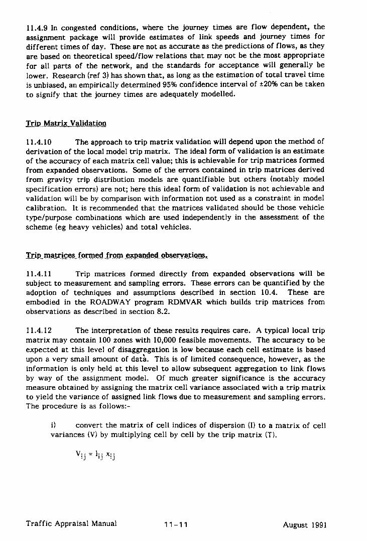
L

11.4.9 In congested conditions, where the journey times are flow dependent, the assignment package will provide estimates of link speeds and journey times for different times of day. These are not as accurate as the predictions of flows, as they are based on theoretical speed/flow relations that may not be the most appropriate for all parts of the network, and the standards for acceptance will generally be lower. Research (ref 3) has shown that, as long as the estimation of total travel time is unbiased, an empirically determined 95% confidence interval of 220% can be taken to signify that the journey times are adequately modelled.

Trip Matr&_Validation

11.4.10 The approach to trip matrix validation will depend upon the method of derivation of the local model trip matrix. The ideal form of validation is an estimate of the accuracy of each matrix cell value; this is achievable for trip matrices formed from expanded observations. Some of the errors contained in trip matrices derived from gravity trip distribution models are quantifiable but others (notably model specification errors) are not; here this ideal form of validation is not achievable and validation will be by comparison with information not used as a constraint in model calibration. It is recommended that the matrices validated should be those vehicle type/purpose combinations which are used independently in the assessment of the scheme (eg heavy vehicles) and total vehicles.

Trip_matrice,~formed ,fr,fm -ended., obervations.

11.4.11 Trip matrices formed directly from expanded observations will be subject to measurement and sampling errors. These errors can be quantified by the adoption of techniques and assumptions described in section 10.4. These are embodied in the ROADWAY program RDMVAR which builds trip matrices from observations as described in section 8.2.

11.4.12 The interpretation of these results requires care. A typical local trip matrix may contain 100 zones with 10,000 feasible movements. The accuracy to be expected at this level of disaggregation is low because each cell estimate is based upon a very small amount of da&. This is of limited consequence, however, as the information is only held at this level to allow subsequent aggregation to link flows by way of the assignment model. Of much greater significance is the accuracy measure obtained by assigning the matrix cell variance associated with a trip matrix to yield the variance of assigned link flows due to measurement and sampling errors. The procedure is as follows:-

i) convert the matrix of cell indices of dispersion (I) to a matrix of cell variances (V) by multiplying cell by cell by the trip matrix ET).

'ij = 1;; Xij .t


ii) load the matrix of cell variances onto the highway network using the trees used to load the trip matrix in the assignment model. Beware of number overflows here: the variance of a link flow is likely to be a very large number which may well overflow the space allocated in the assignment program. Should this occur, factor the variance matrix by dividing by 100 and try again; remember to factor the answers up again.

iii) the resultant output is the variance of the assigned traffic flow on each link due to measurement and sampling error in the trip matrix. No allowance is included for specification errors in the assignment model.

A summary of the results of this assignment should be included in the validation report. This summary should cover all the cordons and screenlines for which count data is available in disaggregate form along with selected links and corridors which are important in the scheme appraisal. The overall accuracy of cordon and screenline by the assignment model will be minimised by the amalgamation process. Alternatively, a sector compression (see 11.4.17) may be preferred, particularly where independent observations permit a comparison.

11.4.13 The approach to validation with local model trip matrices produced by gravity trip distribution models is different to that for observed data trip matrices: this is because the model estimates are affected by model specification error, which cannot be quantified, as well as by measurement and sampling errors, which can. The ideal validation can be approached, however, by the adoption of an accuracy measure based upon the errors in the trip matrix due to measurement and sampling using the techniques and assumptions described in section 10.4. Once again the procedure described in 11.4.12 should be used to aggregate the data to a meaningful level.

11.4.14 To give an absolute measure of the significance of the estimates produced by gravity trip distribution models, it is necessary to compare the model output with information which was not used as a constraint in the model calibration. This information can be classified under two headings:

i) information derived from observations to which the model was fitted but not constrained; and

ii) information from independent observations.

I1.4,55 The data available from observations to which the model was fitted but not constrained will depend upon the method of calibration and the precise constraints apphed. Partial matrix calibration is constrained, in RDGRAV2 and traditionally, to the total trips from and to the observed cells in each row and column, and some function of the trip length distribution of the trips in the observed ~~11s. This Ieaves the individLla1 zone to zone movements which have not been used as a constraint. Synthetic trip end calibration is constrained, in RDGRAV2 and tr -1dit ionall>, ec the input e.u~-nally derived trip ends and a function of the trip IL:lg~h diistribiitim of the 0bswvation.S.


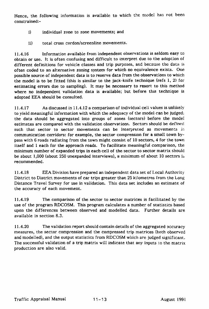
Hence, the following information is available to which the model has not. been constrained:-

i) individual zone to zone movements; and

ii) total cross cordon/screenline movements.

11.4.16 Information available from independent observations is seldom easy to obtain or use. It is often confusing and difficult to interpret. due to the adoption of different definitions for vehicle classes and trip purposes, and became the data is often coded to an alternative zoning system ,for which no equivalence exists,, One possible source of independent data is to reserve data from the observations to which the model is to be fitted (this is similar to the jack-knife technique (refs 1, 2) for estimating errors due to sampling). It may be necessary to resort to this method where no independent validation data is available; but before this technique is adopted EEA should be consulted.

11.4.17 As discussed in 11.4.12 a comparison of individual cell values is unlikely to yield meaningful information with which the adequacy of the model can be judged: the data should be aggregated into groups of zones (sectors) before the model estimates are compared with the validation observations. Sectors should be defined such that sector to sector movements can be interpreted as movements i:: communication corridors: for example, the sector compression for a small town by- pass with 6 roads radiating from the town might consist of 10 sectors, 4 for the town itself and 1 each for the approach roads. To facilitate meaningful comparison, the minimum number of expanded trips in each cell of the sector to sector matrix should be about 1,000 (about 250 unexpanded interviews), a minimum of about 10 sectors is recommended.

11.4.18 EEA Division have prepared an independent data set of Local Authorita, District to District movements of car trips greater than 25 kilometres from the Long Distance Travel Survey for use in validation. This data set includes an estimate of the accuracy of each movement.

11.4.19 The comparison of the sector to sector matrices is facilitated by the use of the program RDCOSM. This program calculates a number of statistics based upon the differences between observed and modelled data. Further details are available in section 8.3.

11.4.20 The validation report should contain details of the aggregated accuracy measures, the sector compression and the compressed trip matrices (both observed and modelled), and the output statistics from RDCOSM which are judged significant. The successful validation of a trip matrix will indicate that any inputs to the matrix production are also valid.


Validation of ,.Assimed kink Flows

11.4.21 As the output of the last model in the chain, the assigned link flows are doubly important because they represent not only the output of the assignment model, but also the final output by which the performance of the complete model will be judged. The purpose of the assignment model in the base year is to predict link flows which are compatible with observed counts. To achieve this, a fitting procedure may be adopted which utilises count information for a selection of links in the area of interest as the basis for choice between alternative assignment techniques or parameters (see Section 9.6). The output link flows will reflect not only the errors of the assignment model itself, but also those inherited from the input trip matrix and road network.

11.422 To validate the traffic flows estimated by the assignment model the model output should be compared with count information reserved from that assembled for the model calibration (see section 9.6). The number of validation counts required will depend upon the scale of the model: for very small schemes comparison with 10 counts or less may suffice, for a typical scheme 20 counts is the likely minimum with many more points being added as the scale of the study increases. Where insufficient count data exists to permit both calibration and validation comparisons of the order required, additional counts should be undertaken. Counts of relatively short duration (eg a 4 hour manual count) will provide sufficient accuracy (the accuracy of counts of short duration is referred to in section 6.3).

11.4.23 The validation comparisons should be tabulated in the validation report. The estimated accuracy of the observations should be included in the tabulation (the 95Ox1 confidence interval is a useful measure) along with the estimated accuracy of the modelled flows due to measurement and sampling errors in the trip matrix when available. Example 11.1 illustrates a possible method of presentation of this data.

m_s__e_nt_Year Validat1oS

11.424 Where the trip information used in a traffic appraisal relies largely upon observations taken more than about 6 years ago it will be necessary to ensure that this information is still valid. This will be achieved by producing a forecast of the current situation and comparing the forecast link flows with count information.

11.4.25 The current year trip matrix should be derived using the appropriate forecasting technique described in section 12.3. It should be assigned to a current year network using the chosen assignment technique.

11 p4.26 The count information assembled should cover the area of interest of the study and should be grouped into cordons and screenlines whenever possible to facilitate comparison. Repeat counts at stations used in the original model calibration will be particularly useful. Relatively short duration counts (eg a 4 hour manual count) will be sufficient as long as the accuracy attained will allow meaningful comparison. The number of counts should be similar to those required under 11.4.22


11.4.27 These validation comparisons should be tabulated in the validation

report. The accuracy of the observations should be included in the tabulation (the 95% confidence interval is a useful measure).


r,--

EXAMPLE 11.1

VAUDATION RESULTS PRESENTATION OF ASSIGNED LINK FLOW Both a tabular and graphrca! presentatron should be presented

Tabular presentatton:

Comparrson of modelled and observed traffic flows (12 hour September 1980 weekday bast

Traf f t c Count lnformat ion

95% Confidence

Road Name Link TYW Duration Count Interval Modelled Ltn

Number of 12 hour flow flow

High Street 101-112 MCC 4 hr 6,400 16.700- 22,100 18.100

Low Road 121- 110 ATC 7days 17,500 10,900 - 12,100 12,300

Median Avenue 93- 57 ATC 7 days 15,900 15,100- 16,700 15.100

Coast Road 61-73 MCC 12 hr 9.900 9,000- 10,900 10.800 ~-_l__ll___

GraphIcal presentatton

22

1

T 95% Conftdence Interval

Y 1

of observattons shown

\I

Modelled Flow <

5

E L Ty Median -Avenue

C E 14-

v 3 0 =

I Low Road Ta

i Coast Roa

I “--- _

I i-----


11.5 VALIDATION OF THE NATIONAL MODEL OF LONG DISTANCE MOVEMENTS

11.5.1 The validation of the National Model of Long Distance Movements was undertaken for the Department by a team of consultants who had not been involved in the development of the model. The validation was undertaken in two parts. A

transportation consultant examined the output matrices and compared them to the calibration data and to other independent survey data (the external validation). A second (academic) consultant carried out a technical audit of the model specification, and the input data, and estimated the accuracy of the model output (the internal validation).

11.5.2 The validation using statistical techniques developed for this manual in the light of SACTFU’s advice, showed that the model did not hold out the full promise of the calibration stage. The academic consultants, for example, commented in their report:

“Whilst the evidence for the accuracy of the input data and of the fitted model may appear alarming at first sight, this may be something one has to get used to in transportation modelling. No similar transportation study in the country (and we suspect anywhere else in the world) has been subject to such detailed scrutiny as has the National Model and its predecessor, the Regional Highways Traffic Model. Transportation planning will have to recognise that the kinds and magnitudes of errors presented in this report are likely to arise in very many applications - and greater attention will have to be paid to getting clean data and an appropriate model specification”.

11.5.3 The transportation consultants noted that the passing or failing of various goodness of fit tests they had carried out could not be the final work in deciding whether the results were suitable for a particular practical purpose: the local scheme teams must rely upon criteria relevant to their particular problems. The consultants did, however, conclude that specific parts of the matrices were for practical purposes unsatisfactory; and show that there were biases in different parts of the country; and that the accuracy in different areas did very much depend on whether the survey data directly contributed to the model results in that area.

11.5.4 The consultants’ recommendations to the Department were:

i) The matrices should be made available to allow scheme teams to decide whether to use them in particular local studies.

ii) The Department should issue a practical methodology so that local teams can estimate the accuracy of each National Model cell in the zoning system of a particular local study, a method now being available from this project.


iii) The National Model results could be considered by local teams for use in studies for long distance trips where the smoothing effect of the model could make its estimates more reliable than the observed calibration data: any use of the model in local studies would require validation using the observed calibration data, this validation should seek to ensure no significant biases are present in a particular modelling needs.

iv) The National Model results, with their associated accuracies, have a role as a “prior model” (ie pilot study) for local traffic study design. Analysis at a model design stage of errors in relation to local requirements would assist in defining supplementary data and modelling needs.

VI In order to gain a more thorough knowledge of how and where the National Model can be applied, experience of local use and validation of the model should be collated centrally.

vi) Because there is still some uncertainty as to how well the National Model fits areas other than those to which it was fitted, it is recommended that the Department undertakes comparisons against District to District matrices based on the independent Long Distance Travel Survey (LDTS) data. Because of the national coverage of LDTS this would provide more conclusive evidence than the validation given by the independent data sets in this study. Consideration should be given to merging those LDTS matrices with the National Model matrices to improve the accuracy of long distance travel data.

vii) Because the inherent statistical error of the distribution model and the trip end estimates is high, it is unlikely that further development of the National Model is worthwhile. It is therefore recommended that no further major development is undertaken except to meet the needs of a specific local study. However, prior to issue of the matrices, it will be necessary to correct them in some way to take account of inconsistencies, particularly those related to trip ends, which were found during the course of the “internal validation”.

viii) Given the inherent error of the model, it is unlikely that it could be applied satisfactorily in a forecasting mode for scheme appraisal. It is also unlikely that it could be used to forecast differential traffic growth by region. It is therefore recommended that the National Model should not be used to model future year trips.

11.5.5 The Department has accepted the recommendations of the consultants. The full results of the validation are reported in refs 4 and 5.



1. Miller R G “The Jackknife - a review”, Biometrika 61, 1974, ~1-15.

2. Bissel AF and Furguson R A “The Jackknife - Toy, Tool or Two-edged Weapon?, The Statistician, Volume XXIV Number 2, June 1975, p79-100.

3. Van Vliet, unpublished report of the study by Greater Manchester Council and ITS of Leeds.

4. The Internal Validation of a National Model of Long Distance Trips; H R Kirby. J D Murchland; Technical Note 95, April 1982; Institute of Transport Studies, University of Leeds.

5. Validation of the National Model of Long Distance Trips: Final Report: May 1982: Howard Humphreys & Partners in association with Transportation Planning Associates and the Institute for Transport Studies, University of Leeds.




12.1 THE DEPARTMENT’S VIEW OF THE FUTURE

12.2 WITHDRAWN(was NATIONAL ROAD TRAFFIC FORECASTS)

12.3 LOCAL FORECASTING PROCEDURES FORUSE

IN TRUNK ROAD APPRAISAL

12.4 THE TREATMENT OF UNCERTAINTY IN TRAFFIC FORECASTING

12.5 LOCAL FORECASTS & NATIONAL CONSISTENCY



12.1 THE DEF’ARTMENT’S VIEW OF THE FUTURE

General

12.1.1 New road schemes represent a major investment by the country for the future: once a road is built it will last for many years. New road schemes also take several years to plan, discuss, and construct. For both these reasons it is necessary

to estimate the future traffic flows which will use a new or improved road. It would not be sensible to construct a road which failed to meet its objectives soon after opening.

12.1.2 The need for credible forecasts of traffic in future years is greatest in the case of urban appraisals, where it is important to know, and present to the public, the impact the scheme will have when it is implemented. There are also the schemes where conditions on the network can be expected to change over the foreseeable future, and the implications for the economic and environmental assessments must be considered. Some guidance on the choice of future years is given in section 12.3

12.1.3 But the Department has also declared its commitment to build roads only where there are pressing current problems. Because traffic forecasts are subject to considerable uncertainty, it is not a robust strategy to bring forward to construction schemes which are justified solely on traffic needs well into the next century. In practical terms, construction to meet pressing current problems means construction to provide relief where traffic problems are now evident or are expected by about the time a scheme is opened because of definite events on the planning horizon (eg opening of a neighbouring scheme or a major land use development).

12.1.4 Forecasts of traffic on a new or improved road, and on roads which will be affected by changes elsewhere, are essential to both the design and the assessment of a scheme. These forecasts consist of two main elements: the extent to which traffic would divert now to the new or improved road, and the expected growth in traffic. This chapter is primarily concerned with the second element, the actual growth of traffic. The SACTRA report on RHTM (ref 1) recommended that the Department maintain a central oversight of forecasts used locally. This is because the trunk road network is a national system of through routes, competing for a common budget, which should be planned on the basis of common assumptions about traffic growth.

12.1.5 This chapter describes the mechanisms for ensuring that local forecasts of traffic are consistent, one with another, while sharing a common basis with the National Road Traffic Forecasts (NRTF) (ref 2).

Traffic Appraisal Manual 12- 1 August 1991

Traffic Appraisal Manual November 1997 12-3

SECTION 12.2 HAS BEEN WITHDRAWN,

SUPERSEDED BY THE 1997 NATIONAL ROAD TRAFFIC FORECASTS

12.3 LOCAL FORECA!STING PROCEDURES FOR USE IN TRUNK ROAD APPRAISAL

General

12.3.1 Regional Offices and headquarters divisions were fully consulted over the forecasting procedures described in this section. The procedures allow central oversight of local forecasts (reference SACTRA recommendation 8) but are responsive to local variations. (The subject of local forecasts and national consistency, which mainly concerns larger schemes, is discussed in 12.5). These procedures are mandatory and must be followed by all those carrying out trunk road appraisals. Those appraising small schemes are particularly referred to 12.3.16(i) and (ii) and 12.3.21 of this section.

Forecasting From Different Bases

12.3.2 Data used for forecasting purposes is available for a number of different bases. Tables 12.1 and 12.2 contain the appropriate economic parameters and indices of vehicle travel which should be used to convert between temporal bases.

Future Road Network

12.3.3 The Department’s current road programme is published in the White Paper ‘Policy for Roads: England 1983 (CMND 9059). The national road network progressively contains these road schemes in future year networks according to their planned timing, until, by 2001, the entire preparation pool is entered (except schemes under review). This implies an average expenditure on roads over this period slightly below the current rate whilst even the low growth assumption in the National Forecasts assumes a small growth in GDP over this period. The national networks therefore are again realistic but cautious as discussed in section 12.2.

12.3.4 However, whilst these networks represent the most reasonable scenarios for the national network, the significance of some of these assumptions must be considered during individual studies. Where a scheme under appraisal is likely to be significantly affected by a proposed neighbouring scheme, then the scheme should be tested with the neighbouring scheme in and out of the future network or at an alternative timing. Such testing should be reported in Technical Appraisal Reports (TARS), and if the integrity of one scheme stands upon the existence of another this must be clearly stated.

Traf fit Appraisal Manual 12 - 5 August 1991

TABLE 12.1

Index of Traffic (1976 = 1001

Year

1976

1981

1983

Year

1976

1980

1981

1982

1983

cars & Taxis

100.0

102.8

107.2

108.2

116.6

117.4

123.9

126.9

Light Goods

Vehicles

<30 cwt ULW

100.0

101.8

104.7

104.1

108.6

110.1

112.1

112.9

Gross

Danestic

Product

(GDP)

per head*

100.0

102.6

105.7

108.3

105.6

103.6

Retail

Price

Index

(RPI)

100.0

115.8

125.5

142.3

167.9

187.8

203.9

213.3

other Goods Vehicles

>30 cwt ULW

100.0

98.5

102.7

104.0

103.7

102.3

99.4

99.8

All Motor

Vehicles

100.0

102.2

106.5

107.4

114.5

115.2

120.4

122.9

Fuel Prices

fin

Behav-

ioural

(pimp price)

100.0

92.6

81.4

94.3

102.4

109.1

107.6

109.9

real terms)

Resource

(net of

tax)

100.0

92.6

79.8

101.7

108.4

100.5

97.1

99.1

Source: Transport Statistics GB 1973-1983

TABLE 12.2

Recent Chanqes in Economic Parameters (1976 = 100)

Road

Ccmstruc-

tion

Price

Index

(RCPI)

100

119

148

183

238

217

224

229

* Real values of time and accidents costs should be assumed to vary in line with those of GDP per

head.

Sources: United Kingdom National Accounts, C-W; Monthly Digest of Statistics, CSD; Department

of the Envircrunent (SC Division); Transport Statistics GB.

Traffic Appraisal Manual 12 - 6 August 991

12.3.5 There are a few schemes and comprehensive route improvements in the roads programme which may have impacts on schemes in more than one region. In general, these schemes should be appraised by the most appropriate region without regard to administrative boundaries and in consultation with headquarters divisions. In the rare cases where this is not practical because major choices in route for large volumes of traffic over long distances are involved, agreement should be reached with EEA and the other affected regions on a common approach. Chapter 13 describes operational appraisal techniques which can be used in these cases.

Choice of Future Years

12.3.6 Where a traffic model is being used in a study, assignments in the opening year and possible other future years will have to take place to allow the estimation of flows on the network required by the economic and operational appraisals. For simple schemes the opening year will suffice; for more complex cases, especially urban appraisals, assignments will be required for other future years as well. Results should be presented for the opening year and, where appropriate, for the final modelled future year.

12.3.7 An estimate of traffic on a new road in the first year of opening is required by TRU 608 for public consultation purposes and an assignment should normally take place for this year. The flows on links for years required by the operational appraisal, for low and high growth, may be calculated simply by using the local growth factors to be input into COBA (see 12.3.22) providing that link speeds are not adjusted in future networks and there is no major “step function” (see 12.3.4) to be considered. This is because routes through a network remain constant under these conditions if temporally stable route choice coefficients are used. (This does not imply that speeds do not change in future years, only that the routes which traffic takes do not change as a result of any speed changes. This is a shared assumption with COBA which does not consider assignments to change between flow groups, nor between years except for those in which a fresh assignment is input; but COBA does change speeds for all years in all flow groups when undertaking economic calculations).

12.3.8 One future year other than the first year of opening should be considered for networks where link speeds are adjusted in future years (eg capacity restrained assignments). As half the economic benefits from a scheme usually arise in the first ten years, and earlier years are less uncertain to forecast, an assignment ten years after opening may be considered. This should generally be back projected by half the difference between the year of opening assignment and second assignment year (for example, the first assignment covers years l-5, the second 6-30). The local growth factors input into COBA applied to the relevant assignments may again be used to estimate the flows on links required in any other year. (Common flow estimates between economic and operational appraisal also result).


12.3.9 If a number of small schemes are being assessed, then their interaction should be taken into account. Forecasts of traffic at different stages in the implementation of the overall strategy will be required, as each individual scheme is opened. This is requisite for the economic assessment, and the steps to be followed in the

evaluation of a series of schemes are clearly laid out in the COBA manual. This procedure would also be useful for urban schemes as their wider implications would then be better understood.

123.10 Where a major “step function” in road user costs is likely to occur, usually due to the projected opening of a neighbouring scheme, further assignments should take place on each occasion (usually with and without the change, see 12.3.4). Only major land use changes should raise the need for further modelling. The effects of land use changes are usually relatively minor and generally best considered as part of operational appraisal (see Chapter 13).

Outnut from the National Sub Models

12.3.11 The national sub models are described in Chapter 7.

12.3.12 Local forecasts of car ownership, together with forecasts of cars per person, have been produced which agree fully with those produced nationally. The estimates of cars per household and the proportions of households in each of the 3 car owning categories are consistent.

12.3.13 Local zone forecasts of private vehicle trips have been produced using compatible car ownership estimates.

12.3.14 Outputs from the National Sub-Models are available as described in Appendix 20.1.

Future Year Route Choice Coefficients

12.3.15 The route choice coefficients fitted in the base year can generally be used in producing assignments for economic appraisal for ail future years. Sensitivity testing may take place as judged necessary using other route choice coefficients (see section 12.4). The choice of future year coefficients is fully discussed in section 12.5.

Forecastinn Procedure for the Different Model Forms - Private Vehicles

12.3.16 A summary description of the model forms available for trunk road appraisal is contained in section 5.6. The following procedures are applicable for the 5 travel demand model forms described for private vehicles only. The “National Forecast Adjustment Factor” is explained in section 12.5. Forecasting methods are described in Appendix 12.4.


c

i) Simnle Link Counts and Growth Factors NRTF forecasts of the increase in vehicle kilometres should be used as growth factors.

ii) Observed Origin and Destination Matrices and Growth Factors

a. NRTF forecasts of the increase in vehicle kilometres should be used as growth factors in the assessment of small schemes (ie “Form 502” schemes) as defined in 19.1;

b. Uniform local growth factors may be used where growth is considered by the traffic engineer to be broadly homogeneous over the study area. The growth factor should be the trip end growth over the scheme study area or, for small schemes, the effective area of influence of the scheme (normally l-3 counties): the national forecast adjustment factor must be applied; or

C. Furness procedures may be used based on the growth in trip ends in individual zones; the national forecast adjustment factor must be applied.

iii) Base Year Synthetic Matrices with Growth Factors based on National Sub-Models

As in ii) above.

iv) Base Year Synthetic Matrices based on Local Planning Data and Local Sub-Models with Growth Factors for Forecasting

As in ii) above. In addition, the growth in trip ends should be controlled at Local Authority District Level to be compatible with those of the National Sub-Models. It is desirable that local car ownership and planning data are close to national estimates at District Level.

v) Model Forms iii) or iv) with Future Year Redistribution When a future year re-distribution or cost function iteration is to be carried out the following steps should be taken:

a. the national forecast adjustment factors should be applied:

b. the base year generalised cost parameters must be used. This is because any future year effects have already been embraced in the trip end models and the national forecast adjustment factors; and

C. the growth in vehicle kilometres should be inspected and compared with the national forecasts to ensure that the effects of redistribution are reasonable.

Traffic Appraisal Manual 12 - 9 August 199 1

12.3.17 Changes in total vehicle kilometres in a traffic model are acceptable when arising for the following reasons (extreme effects should be referred to EEA Division):

i) because of the presence of new schemes; or

ii) because of redistribution (but inspection should be carried out as described in v) c. above); or

iii) in sensitivity tests using differing route choice coefficients; or

iv) because of capacity restrained modelling effects.

12.3.18 It should be noted that in all cases where local forecasts are used the national forecast adjustment factors are applied.

12.3.19 Private vehicle trip end growth may be applied either to separate trip purpose matrices or in total. Models which do not hold trip information by purpose, and most smaller models based upon trip matrices formed by expanding observations, should adopt the latter course. Where local private vehicle trip end growth is applied it is necessary to prepare local growth factors for COBA. Where separate trip purpose matrices are used, the local split between travel in course of work and for other purposes will also have to be taken into account. A procedure for estimating this is described in detail in chapter 4 of the COBA manual.

12.3.20 Where private vehicle trip end growth is applied to the separate trip purposes recommended in section 8.1, that is:

i) Cars and Vans - Journey to Work; ii) Cars and Vans - On Employer’s Business; iii) Cars and Vans - All Other Purposes; and iv) Goods Vehicles - All Purposes,

these purposes have to be reconciled with the trip ends that are available from the national sub-models for forecasting, that is:

Home-Based Work (HBW); Home-Based Employer’s Business HBEB); Home-based Other (HBO); None-Home-Based Employer’s Business (NHBEB); and Non-Home-Based Other (NHBO)

As there is no trip end model for vans on employer’s business (or for goods vehicles) the National Road Traffic Forecasts (NRTF) must be used. The formation of the future year matrices can be undertaken as follows:

i) Cars and Vans - Journey to Work The growth factor is the trip end growth of the Home Based Work purpose in the national trip end files. The National Forecast Adjustment Factor must be

applied.


ii) Cars and Vans - On Emnlover’s Business The future year matrix is formed from 3 components:

a. Home-based employer’s business (HBEB)

b. Non-home-Based employer’s business (NHBEB)

C. Vans on employer’s business

The matrix must be formed by the addition of 2 separately forecast matrices, the second matrix being that of vans on employer’s business which it was explained in 8.1 would have to be maintained separately for forecasting purposes. The growth factor for the first matrix is the trip end growth of a. and b. combined from the national trip end files. The National Forecast Adjustment Factor must be applied. The growth factor for the second matrix is obtained from the NRTF (no adjustment factor is required).

iii) Cars and Vans - All Other Furnoses The matrix growth factor is produced by combining the Home Based Other and Non Home Based Other purposes from the national trip end files to provide the forecast trip end growth. The National Forecast Adjustment Factor must be applied.

iv) Goods Vehicles - All Purnoses As described in 12.3.21

Forecast Procedure for the Different Model Forms - Commercial and Public Service Vehicles

12.3.21 The NRTF growth factors should be used in all cases for light commercial vehicles, other goods vehicles and public service vehicles. This control may be applied uniformly over the study area, or at District or County level to allow for local variation where growth is not expected to be spatially homogeneous. Disaggregation of other goods vehicles (OGVs) greater than 30 cwt to estimate the proportion over 25 tonnes may be carried out on a link basis after assignment (though national estimates should be used with caution, see ref 31, but unless special attention has been paid to sampling, or a special modelling approach has been adopted (see section 8.1), this should not be attempted on a matrix basis (see section 8.5).

Calculation of Local Annual Growth Factors for InDut to COBA

12.3.22 Traffic is split into 5 standard classes in COBA 9 (Chapter 4 of the COBA Manual) and different values of time and vehicle operating cost are attributed to each of these 5 vehicle classes. The classes are:

1. Cars: including taxis, estate cars and light vans with rear windows.

Traffic Appraisal Manual 12- 11 August 1991

2. Light Goods Vehicles (LGV): all goods vehicles up to 3.5 tonnes design gross vehicle weight. This includes light vans and light goods vehicles and equates approximately to up to 30 cwt unladen weight (in practice, vehicles with 2 axles fitted with a total of 4 tyres).

3. Other Goods Vehicles (OGV): All goods vehicles over 3.5 tonnes design gross vehicle weight (in practice, vehicles with 2 axles fitted with more than 4 tyres, and vehicles with more than 2 axles. This equates approximately to greater than 30 cwt unladen weight). This category can be split as follows:

i) Vehicles less than 25 tonnes design gross vehicle weight identified as less than 4 axles;

ii) Vehicles greater than 25 tonnes design gross vehicle weight identified as 4 axles or more.

4. Buses and coaches: including works buses but not mini-buses excluding caravans or other types of car and trailer.

12.3.23 An option exists in COBA to input local annual growth factors for each of the vehicle classes, otherwise the NRTF are used (see Chapter 4 of COBA manual). For trunk road appraisal, local growth factors for Class 1 (of 12.3.22 above) must be used where the forecast trip matrices are based on growth derived from the national trip end files: NRTF growth should be used for the other vehicle classes. The proportion of travel within Class 1 which is carried out in course of work can also be varied over time within COBA 9. Where local forecasts have been based upon separate trip purposes (see 12.3.19) then the varying proportion of travel in course of work should be allowed for in COBA evaluation (see Section 4 of COBA manual).

12.3.24 Local growth factors must be constrained to Local Authority District level trip end growth with the national forecast adjustment factor applied (see section 12.5). However, the national trip ends models are only run at the (census) years 1981, 1986, 1991 for which there is forecast planning data. Intermediate years should be produced by interpolation between these years.

Reuorting the Forecasting Method Used

12.3.25 The forecasting method used, the way in which control to NRTF has been achieved and the network changes assumed in the scheme traffic forecasts should be reported to EEA when the economic evaluations are submitted. The report may either be appended to the Local Model Validation Report or included in the report on the traffic inputs to COBA.



EXAMPLE 12.1 HAS BEEN WITHDRAWN,

SUPERSEDED BY VERSION 10 OF THE COBA PROGRAM


.

EXAMPLE 12.1 HAS BEEN WITHDRAWN,

SUPERSEDED BY VERSION 10 OF THE COBA PROGRAM

12.4 THE TREATMENT OF UNCERTAINTY IN TRAFFIC FORECASTING

L Introduction

12.4.1 An outcome is considered uncertain when it cannot be assigned a probability. Traffic forecasts are uncertain; the total uncertainty of the model output is a combination of the uncertainty of the forecasting process, the statistical errors of measurement, sampling and parameter estimation, and the specification errors of mathematical models which simplify the complexities of the real world. The uncertainty of the overall estimate must be recognised when traffic study results are used in decision making.

12.4.2 The treatment of uncertainty in traffic forecasting adopted by the Department relies upon the use of a range of forecasts which have been adopted as a matter of policy for trunk road planning purposes. The range has been defined by the adoption of alternative views of the economic future of the nation as described in the National Road Traffic Forecasts (see section 12.2). The alternative results form the basis for decisions.

12.4.3 This TAM is not concerned with giving advice on decision making but with assembling information as an input for decision making. For the purposes of this section, however, three stages of decision making under uncertainty within traffic appraisal will be assumed:

i) the identification of the range of feasible traffic estimates which it is sensible to consider;

ii) the identification and evaluation of options appropriate to these estimates; and

iii) the selection of the preferred option.

L

It is the task of those carrying out traffic appraisals to identify the range of feasible traffic estimates and to provide the data upon which the evaluation of the options proposed can be based.

12.4.4 This section first considers the treatment of uncertainty in forecasting adopted by the Department, and how this is used to identify the range of feasible traffic estimates. It then describes the forecasting errors which cause the uncertainty, and sensitivity tests which may be used to describe the uncertainty.

Identifying the Range of Feasible Traffic Estimates

12.4.5 As discussed in section 10.1, the current state of the art of the treatment of uncertainty put forward in this manual is in two partx-

i) The assessment of errors in the base year (Chapter 10); and


ii) the treatment of uncertainty in forecasting.

With the aid of the techniques described in Chapter 10, it is possible in many cases to directly estimate (using standard statistical methods) the accuracy of model

estimates in the base year. When forecasting, however, a number of assumptions of

unknown accuracy are made and the probability of any outcome cannot be directly assessed. To take account of uncertainty in forecasting, the Department has adopted as a policy a range of forecasts of the national growth in vehicular traffic.

12.4.6 The range of forecasts in the NRTF has been produced by inputting alternative economic scenarios to two forecasting models. The resulting forecasts represent a realistic view of the future. It is not intended that the NRTF range should be further widened by the superimposition of measurement and sampling errors from the base year data or errors from local forecast parameters. In this way the Department’s procedures are designed so that forecasting errors are correlated between appraisals and hence across all schemes. Funds can therefore be fairly allocated in the knowledge that assessments are based upon the same Departmental view of the future.

12.4.7 The procedure for producing forecast year traffic flows for any year is therefore a straightforward growthing up of base year counts or matrices using the two sets of indices (high and low growth) from the NRTF (or local growth factors based on the national trip end models) to give the full range of estimated future traffic by the procedures described in section 12.3.

Forecastinrz Errors

12.4.8 Forecasting errors are the difference between the predicted future values of input data required by the model, and the outturn values. Predictions of future year values of inputs are uncertain, that is the precise future value of any variable is unknown, and the probability of any particular outcome cannot be exactly assessed.

12.4.9 Model inputs for which future year forecasts are required when using a model in predictive mode can be categorised as:-

i) parameters which are assumed to be stable over time, ie constants;

and

ii) parameters where future values are different to current values, ie

variables.

Examples of the former are calibrated model parameters; and of the latter are Gross Domestic Product (from which incomes are estimated), petrol prices, values of time for different purposes, population forecasts and the highway network. Future year values of all these parameters are subject to forecasting errors. When a parameter which is assumed to be a constant is, in fact, a variable this might alternatively be called a model specification error.


‘d

d

L

L

124.10 Forecasting errors are likely to increase with the time span of the forecasts and, as such, will be minimised by reducing the forecasting horizon to the shortest possible.

Sensitivitv Tests

12.4.11 Sensitivity tests, which were introduced in section 10.6, may be considered in three categories:-

i) small perturbations of the model parameters used in any of the sub-models to ascertain the sensitivity of each sub-model to the choice of parameter value (particularly relevant to the assignment model);

ii) selective sensitivity testing where a high and a low value are chosen towards the extremes of the feasible range of values for each parameter to ascertain the resulting range; and

iii) systematic sensitivity testing (SST). A structured approach to sensitivity testing which seeks to paint a picture of the likely range of outcomes by running a set of models with each parameter carefully chosen from a range.

12.4.12 Selective sensitivity testing (where a high and low value is chosen for each parameter, and the model run) is the approach adopted in both the National Road Traffic Forecasts and the economic evaluation using COBA. Whilst useful for identifying the full range of feasible outcomes, the information gained does not necessarily assist in determining whether the effects of alternatives are significantly different, and hence, with the making of decisions.

12.4.13 Work is at present being examined in EEA on systematic sensitivity testing (SST). In this procedure, which is an outcome of the research into uncertainty carried out by EEA division (as EH), input data and model parameters are purposively selected from a range of possible values and the model run. This process is repeated a small number of times so that the likely range of final link flows and the probability of each occurrence can be described. The process encompasses measurement and sampling errors, model specification errors and forecasting errors: the need for independent tests for each type of error is in this way removed as their joint effect is described. The rationale behind SST is that sensitivity tests should be part of an overall programme of tests used to define the probability of various outcomes not just to identify random or extreme points. The aim, therefore, is to develop a structured approach from which the maximum information can be extracted.


12.5 LOCAL FORECASTS AND NATIONAL CONSISTENCY

Gfznfzral

12.5.1 The Department now has at its disposal a number of tools which allow local practitioners to use both a traffic appraisal technique appropriate to a particular local problem, and to integrate local traffic forecasts into a national framework where direct application of NRTF growth is not appropriate (see 12.3). Not all of the tools are applicable to every case. The tools are:-

i) a national zoning system (see 4.3);

ii) a national network (see 4.4);

iii) a national set of planning data (see 4.5 and 4.6);

iv) the national sub-models of car ownership and trip ends (see Chapter 7);

v) common software for traffic appraisal (see 20.3);

vi) an agreed set of mechanical procedures for forecasting; and

vii) advice provided by this Traffic Appraisal Manual and the COBA manual.

The first four of these tools were first developed during the RHTM project.

12.5.2 It is not possible to ensure that the sum of vehicle kilometres produced by local forecasts equates to that predicted by the national forecasts: to do so would require a national traffic model of a type that is not currently available.

12.5.3 What can be achieved is sufficient commonality of modelling practice to allow decisions on schemes to be made on a rational and consistent basis throughout the country. Schemes under appraisal must therefore share common assumptions about the amount and manner of traffic growth.

Control of Local Forecasts to National Estimates

12.5.4 Central oversight of forecasts and a common approach to forecasting throughout the country is achieved by centrally produced trip end estimates acting as a control on local traffic growth (see 7.3). The estimates are produced by the national sub-models fed by the national planning data set (see 4.6). The planning data set is constrained such that the sum of local zonal projections is constrained to total national projections (eg population). ‘The lowest level zone at which this can sensibly be achieved is Local Authority District level: the national zoning system contains 447 District level zones. Using the same structure in the national sub-models as were used in the NRTF, and the national planning data set, a national set of trip ends can be produced at Local Authority District level compatible with the NRTF.


To make local forecasts of travel completely compatible with NRTF requires one extra factor - the national forecast adjustment factor.

The National Forecast Adjustment Factors

12.5.5 Because the NRTF assume that kilometres per car will vary with the change in real income and petrol price over time, an assumption which the national trip end models do not embrace, compatibility requires that small adjustments have to be made in local forecasting procedures.

12.5.6 To implement the NRTF assumption of changing kms/car, it is not necessary to determine whether this change is to apply to the number of trips or the length of trips or to both: nor is there, yet, any conclusive time series data. Because the factors are small, and because of the costs incurred and the model specification errors introduced by adjusting trip lengths (particularly with respect to observed trip matrices), the adjustment factors are assumed to apply only to trip ends. The national forecast adjustment factors are therefore the factors that control the growth in the total of trip ends from the national trip end sub-model to that of vehicle kilometres forecast in the NRTF.

12.5.7 in addition to the main purpose of the national forecast adjustment factors, the factors also correct for small technical differences caused by the use of different estimating methods in the trip end model and NRTF, eg the effects of grouped estimates. These technical adjustments amount to about 2% of total trips.

12.5.8 The factors are given in Table 7.1. Thus, if the number of trips in the base year were 1.1x106, and in the first year of opening (from Furnessing) were 1.2x106, and the national forecast adjustment factor was 1.02 then growth in vehicle kilometres (excluding assignment and redistribution effects) should be

(1.2 x 106) x 1.02 1.1

The national forecast adjustment factors can be applied directly to the trip ends.

12.5.9 The fitting of route choice coefficients, and their relation with network speeds, was described in 9.6. In some studies it has been the practice not to assume temporal stability of the fitted route choice coefficients where the coefficients of time and distance used were derived from behavioural generalised cost calculations: these coefficients being assumed to be linked to the value of time and the cost of petrol and so to vary with assumed changes in these parameters.

12.5.10 There are a number of arguments for and against maintaining the coefficients fitted at the base year in trunk road appraisal. The main arguments for maintaining the base year values are:


i) the high and low growth forecasts already embrace a cautious and carefully chosen wide range of possible outcomes. The assumption of temporal instability introduces further widening so that the forecast range may resemble, for some schemes, two unlikely outcomes rather than being the maximum range within which it is sensible to plan (see section 12.4). In reality, many compensating effects are likely to drive the forecasts within the predicted range;

ii) cheaper traffic studies result in some cases because the same set of routes, for a given network, can be used for any forecast year and any trip matrix (except where future year network speeds are adjusted eg capacity restraint);

iii) the evidence linking the route choice coefficients with generalised cost is not conclusive (see 9.2). Without time series data proving the hypothesis, many practitioners are reluctant to abandon the fitted coefficients which reproduced the base year traffic flows;

iv) the coefficients of time and distance already depend on network speed coding methods; and

v) the Department is committed to building only where there are pressing current problems (see 12.1): so both decision making, and the discounting process in economic appraisal, should be weighted towards earlier years.

12.5.11 The main arguments against maintaining the base year values are:

i) the resource costs used in COBA change their values with changing GDP and fuel costs. It would be more consistent to allow the behavioural values of time and distance used in estimating rout= to change in the same way;

ii) it is reasonable to expect that if the real cost of motoring rises faster then real earnings than drivers will pay more attention to distance travelled in selecting routes; and

iii) the estimation of the effects of tolls is more straightforward where generalised cost is used.

12.5.12 questions:

Whatever the balance of the above arguments, there are two pertinent

i) is the future relationship of time and distance in the generalised cost formulation very different from that of the base year?

ii) is the adoption of either assumption likely to lead to bias in the appraisal of road schemes?


In practice it is found that the mid-point of future year values of generalised cost are close to the base year values (see figure 12.1); and there is little evidence to suggest that the allocation of funds over the trunk roads programme would differ with the adoption of either temporally stable or changing coefficients.

12.5.13 In most cases it appears adequate to assume that the assignment coefficients remain stable and therefore for a given network, if no congestion occurs, that routes remain unchanged. Bearing in mind the simplicity and economy in maintaining the base year coefficients, it is expected that most studies will adopt this course. However it is advisable to undertake some sensitivity testing as described in section 12.4 (see also 10.6) to ensure that the significance of the assumption is understood.


Traffic

Appraisal

Manual

12 - 23 A

ugust 1991

REFERENCES-CHAPTER12

L.-’ 1. “Forecasting Traffic on Trunk Roads: A Report on the Regional Highway Traffic Model Project”, The Standing Advisory Committee on Trunk Road

Assessment; HMSO, December 1979.

2. National Road Traffic Forecasts 1984; EEA Division Department of Transport, 2 Marsham Street, London SWl.

3. Table 2.4, Transport Statistics Great Britain 1969-1979; Department of Transport, Welsh Office, Scottish Development Department; HMSO 1980.

4. “Report of the Inquiry into Lorries, People and the Environment”, HMSO, 1980.


CHAEYCER 13 : OPEFULTIONAL APPRAISAL

13.1 GENERAL

13.2 EXAMINING THE OPERATIONAL FEATURES OF A SCHEME

13.3 THE TOOLS OF OPERATIONAL APPRAISAL

13.4 THE USE OF CORDON ISOLATION TO EXAMINE CONGESTED NETWORKS

13.5 JUNCTION APPRAISAL

13.6 PREPARATION OF TRAFFIC FIGURES FOR USE WITH OTHER DEPARTMENTAL PUBLICATIONS


Traffic Appraisal Manual Augus-t 1991

CHAPTER 13 : OPERATIONAL APPRAISAL

13.1 GENERAL

13.1.1 Operational Appraisal is a detailed form of Traffic Appraisal which is needed particularly in urban areas. It has two main applications. Firstly, during early stages of building a traffic model it is necessary to examine model output to ensure that results are reasonable. Later on in a study, the operational appraisal should highlight areas where a traffic model (and COBA) is oversimplified so that results from the model can be qualified where appropriate.

13.1.2 Secondly, the operational appraisal should describe the local impact of a scheme so that the strengths and weaknesses of a proposal can be identified (eg are any junctions likely to become overloaded ?I. This will often suggest beneficial amendments to the detailed design such as ancillary traffic management. The appraisal will also identify areas where complementary action will be needed by statutory and other bodies such as Local Authorities or bus operators.

13.1.3 The first section of this chapter sets out a check-list of operational features which may be relevant in examining a particular scheme. The second section describes methods which will be of value in examining the model itself, as well as in assisting understanding of traffic behaviour. The third and fourth sections concern networks and junctions, the latter usually being the kernel of most traffic problems. The final section describes the preparation of traffic figures for use with other Departmental publications and discusses some of the problems inherent at these interfaces.


13.2 EXAMINING THE OPERATIONAL FEATURES OF A SCHEME

h-’

13.2.1 Most features requiring consideration in operational appraisal lie within the vicinity of a scheme. Occasionally, remote features such as signing or an estimate

of increased loadings on unsuitable link roads will require consideration. No checklist of features requiring examination can be exhaustive because the nature of operational appraisal is its case dependence. However the following check-list

contains some common features for consideration many of which can be examined using the tools described later in 13.3 (a full list of references relating to design is given in DTp Circular 4/79, ref 1).

i) Safety: is this option, in its detailed layout, the most cost effective which can be designed ? What are the accident costs estimated by COBA? Could small changes in layout and signing encourage greater volumes of traffic to use roads with lower accident rates or pass through fewer junctions? Can pedestrians be further segregated from traffic?

ii) Network balance: for example, does the relief of one bottleneck (which is not part of a comprehensive route improvement programme) cause longer queues at the next bottleneck thereby reducing the peak period economic benefits calculated by COBA? Do climbing lanes following a long stretch of single carriageway with restricted overtaking provide considerable benefits which are underestimated by COBA?

iii) Pedestrians: Will pedestrian facilities be necessary that will alter the attractiveness of a scheme? For example, a new pelican crossing on a new dual carriageway (thereby negating much benefit); or a new footbridge or subway (with the associated capital cost).

iv) Interacting Junctions: Does the pattern of release of flow from one junction affect another downstream ? (This can be a positive or a negative effect; it can be positive particularly when the downstream junction is of the major/minor type and the minor road flow needs breaks in the major road flow).

v) Access: Are there any restrictions (eg height, weight, turning radii, traffic management policies) which prevent traffic from using the modelled routes? Should some accesses be closed for safety or capacity reasons? Does the scheme attract traffic down undesirable routes to gain access to it? (eg residential areas, unsuitable country lanes, town centre etc).

vi) Junctions: Which junctions, if any, are likely to become overloaded? (Junctions which are likely to become overloaded should be identified in the traffic model).

vii) Planning Policies: Does the scheme close or assist land development options?


viii) Enforcement: Are there any traffic orders (clearways, banned turns, parking, access restrictions, traffic signals, speed limits, etc) which are essential to the viability of the scheme (or a staged opening), for ‘which police agreement is required?

ix) Maintenance: What are the maintenance implications? What traffic costs will be incurred during maintenance ? Maintenance considerations are a major item in decisions on option viability and standards of carriageways and junction provision. (As traffic continues to grow, and the age of the road network increases, maintenance considerations are increasingly important).

x) Staged Onenings: Does a temporary terminal point, which may last many years, have adequate capacity to cope? Do any of the previous nine points have relevance to temporary stages?

13.2.2 When carrying out operational appraisal on new road schemes, it is important to distinguish between those operational features which fundamentally affect the decision on the viability of a scheme (eg demolition of buildings to provide necessary junction capacity); and those features which are marginal details that can be amended at low cost after a scheme has settled in (eg traffic signal settings).


13.3 THE TOOLS OF OPERATIONAL APPRAISAL

13.3.1 There is a range of diagnostic quantities which can be used in appraising the

impact of a scheme. Nearly all can be extracted from a traffic model and are of

assistance in understanding, and explaining to others (see Chapter 151, what a particular scheme would achieve. They are also of value in optimising detailed aspects of particular solutions but, when a choice between alternative solutions is to be made, they must take second place to the formal economic and environmental

appraisals.

13.32 Operational appraisal is by its nature scheme dependent and the responsibility of local practitioners. The following items are amongst those of value:

i) J ournev Times: The estimated journey time for a vehicle using the whole of a new route as against the old. For large schemes this can be done for major sub routes. Figure 13.1 shows how a map can be prepared in critical sections of a network showing speeds.

ii) Maior Volumes: Where a scheme is on a route between two major towns, the volume of traffic between those two towns can be shown. Desire Line diagrams (figure 13.2) showing the origins and destinations of major flows can be plotted (program RDSELC): best results are obtained by grouping traffic into no more than 20 sectors containing zones of homogeneous traffic interest.

iii) “Select link plots” (figure 13.3) as produced by programs RDSELC and RDPLOT, showing the traffic contribution to the network of traffic on a chosen link (usually a major scheme link or a link of interest such as a High Street.) Separate vehicle classes (eg commercial vehicles) or purpose types can be examined if appropriate.

iv) Estimated loadinps that major links may experience over their

economic life can be plotted as in Figure 13.4. This figure can be extended to illustrate the uncertain opening of a neighbouring link (Figure 13.5). The base need not be AADT: it could, for example, be a COBA flow group.

v) Traffic Routes: The routes to certain selected origins (Figure 13.6) used by the model in assignment can be plotted (programs RDTREE and RDPLOT). Centres of major towns, terminal points of routes, or potential sites of major interchanges are commonly chosen.

vi) Junctions: A broad estimate of the capacity of any junctions in the vicinity of the scheme which may become overloaded. (Junctions are discussed in 13.5).

vii) Economic Diagnostics: Use of NETBEN AND MATBEN (see Chapter

14) to illustrate which links, and which movements through the network are gaining respectively benefits and disbenef its.


viii) Network Comparisons: Two loaded networks (eg do minimum and do something) can be compared and plotted such that all links whose volumes change by more than a specified amount can be identified (programs RDCOMP, RDFLOW and RDPLOT). This is a very powerful tool for larger network models.


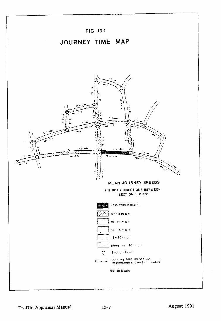
FIG 13-l

JOURNEY TIME MAP

MEAN JOURNEY SPEEDS

(IN BOTH DIRECTIONS BETWEEN

SECTION LIMITS)

Less than 8 mph

10-12 mph

I 12-16mp h

-

f 16-20m p h

L---_-j Mc?re than 20 m p h

0 Sectton limit

c h_ Journey tame on sectlon II-I direct IOn shown ( m mmutes 1

Not to Scale


Traffic

Appraisal

Manual

13-8 A

ugust 1991

FIG. 13.5

SCHEME AND SECTION: M999 BARNBURY- MIDDLEWAYfINCL A777 OPENING OPTION)

lOAD CLASSIFICATION MAIN -URBAN STANDARD: 02 ALL PURPOSE WITH AT GRADE JIJNCTION!

NO HARDSHOULDERS r / . . / HC

32000.

31000

30000

29000

28000

27000

2bOOO

35000

23000

?:I000

22000

2 1000

20000

19000

I8000

17000

16000

~~~_-_____-----------

”

HrI I

Urlcertai. openlncj

LOW nn

i

BROOKFIELD

CROFTDOWN \CARCH wAYo

! KENTISH


- ~_. .-.. ~

NETWORK SELECT LINK PLOT FIGURE 13.3 1

SW ESTATE

BROOKFIELD -96

758


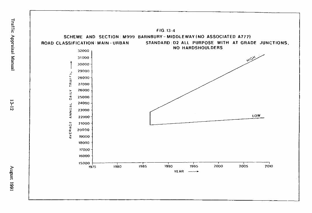
FIG. 13.4

SCHEME AND SECTION: M999 BARNBURY - M I

ROAD CLASSIFICATION : MAIN - URBAN STANDARD

32000

31000

30000

29000

28000

27000

26000

25000

24000

23000

2 2000

21000

20000

19000

18000

17000

16000

15000 l!

DDLEWAY (NO ASSOCIATED A7771

02 ALL PURPOSE WITH AT GRADE JUNCTIONS. NO HARDSHOULDERS

I I 1 I I 1 1 ‘5 1980 1985 1990 1995 2000 2005 2010

YEAR -

6

13.4 THE USE OF CORDON ISOLATION TO EXAMINE CONGESTED NETWORKS

13.4.1 In all traffic models, except the very smallest of less than about 30 zones, the use of cordon isolation software to extract a sub-network from the model being used can provide a powerful tool for the appraisal of difficult areas such as sections of congested network. A cordon matrix can be extracted in ROADWAY using RDSELC. A cordon network extraction program may be available in 1981.

13.4.2 The cordon isolation should be as small as is feasible to surround the problem area. Small models with less than 30 zones or 60 links are highly intelligible and controllable for detailed operational appraisals and embrace all the major influence of the usual features under examination (eg one or two bottlenecks; interacting junctions; a new land use development; terminal arrangements of a new road) which any model is capable of discerning. This is because traffic quickly, but not instantly, disperses over the network (see Fig 13.7) and the difference in delays to traffic at a junction approach at varying traffic loadings is very small providing the junction approach is working a little below capacity. If a junction approach is working near capacity and above, the rate of change of delay with flow is very fast, and so very small changes in flow at junctions well remote from the influence of the scheme can show up as major effects in a traffic model. In reality many minor adjustments take place in traffic demand (ref 2) which remove the major operational problems predicted by traffic models at small flow changes (these small changes in traffic demand do of course carry associated costs to traffic). The analysis of congested networks is described in the TRAFFICQ user manual (see Appendix 13.1).

13.4.3 The time periods for use in such appraisals were discussed in 5.7. Any factored daily matrix (see also 6.10) which will place the design under feasible peak loadings of the type of interest in the area of interest will be suitable. (There is an analogy here with the load testing of structures). Factoring to make the design respond under directional loadings may be injected if required. For small matrices, ad hoc methods of factoring the daily matrix will be sufficient: for example, a factor based on the ratio of peak period flow in the direction being considered to the daily flow on cordon crossing points.

13.4.4 The following two methods are among the approaches suitable for larger matrices. In the first, a peak period matrix may be built at, or compressed to, a very coarse sector level (perhaps 5 sectors of homogeneous traffic interest) and be divided by the daily matrix compressed to the same level: this then gives a directional peak to daily factor for each sector. Each cell in the uncompressed daily matrix can then be factored by the appropriate sector factor (eg there will be 25 factors for a 5 sector system). This coarse sectoring process overcomes peak period sampling problems because the factors are drawn from a data base which contains sufficient interviews during the peak period to derive a directional relationship with the daily matrix.


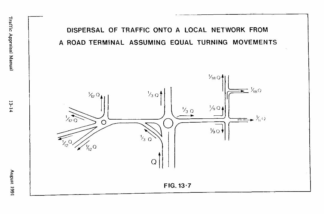
DISPERSAL OF TRAFFIC ONTO A LOCAL NETWORK FROM

A ROAD TERMINAL ASSUMING EQUAL TURNING MOVEMENTS

‘A3 Q I

L

13.4.5 A second method which can be adopted, which is more convenient to apply to synthetic models than to observed data models, is to take “slices” of daily purpose matrices and assemble these into a peak period matrix. In this method, the data base is examined to establish the percentage and direction of trips from each purpose in the time period of interest (and this is sometimes only done for home based journey to work trips). For example, in the morning peak period a substantial percentage of the home based journey to work trips will take place, travelling to work. The morning peak matrix might therefore be of the form:

am peak = al % G/A journey to work + a*% G/AT journey to work

+ bl % G/A home based other + b2% G/AT home based other

+ . .

where G/A =

G/AT =

. . .

generation/attraction matrix

G/A transposed

and al .> a2

This method also overcomes peak period sampling problems.

13.4.6 The choice of model to be used once a cordon matrix and network has been extracted is quite wide (see also 5.3):

i) ii) iii) iv)

Manual or Semi-Automatic Methods. The Cordon Matrix and Cordon Network Model. TRAFFICQ. CONTFZAM.

Manual or Semi-Automatic Methods

L 13.4.7 Manual assignment, or the use of the diversion curve in 9.6 together with calculations of junction delays based on the calculations described in the COBA Manual Section 6.

The Cordon Matrix and Cordon Network Model

13.4.8 This model will generally require minor refitting. It may be necessary to improve the level of model detail within the cordon by means of increased zone and network definition and the use of more complex assignment procedures (ie capacity restraint, multi-routeing). If Burrell multi-routing is used, a substantial number of trees per origin (perhaps up to 100) may be needed with a small number of zones (eg 30) to achieve stability (see 9.5).


Speed-flow curves can have substantial shortcomings in capacity restraint at this level of detail: because they are link based, the sum of flows on links entering a junction estimated by the model may easily exceed finite junction capacities. This can be partially overcome by the use of notional links describing junction delays at critical junctions: delays are then calculated at each iteration considering each junction as a whole. Several commercially available transportation suites do this mechanically but for small networks manual intervention to undertake these calculations can speed up convergence and be profitable in interpreting the behaviour of the network. Manual intervention becomes too time-consuming for networks with greater than about five critical junctions.

TWFICQ

13.4.9 TRAFFICQ (ref 3) was outlined in section 5.5. TRAFFICQ operates at the most detailed level of techniques widely used in the UK, by following individual vehicles through the network and registering their progress through queues; waiting for traffic signals to turn green; waiting for gaps to execute right turns; and so on. For a given traffic demand in a small congested network, TRAFFICQ is suitable for examination of:

i) a new road;

ii) road widenings or flaring of junction approaches or exits;

iii) change in form of junction control or layout;

iv) change in location of a pedestrian facility;

v) introduction of bus lanes, banned turns, one-way systems etc;

vi) the effect of changed traffic demand or behaviour - say from a new industrial estate, superstore, or car park.

13.4.10 One of the virtues of using TRAFFICQ for small networks is that whilst all route choice options (including multi-routeing) are open, a full route choice model does not have to be fitted because manual assignment is used (diversion curves, see 9.6, or other methods external to the program can of course be used): this makes for very fast appraisal. However this property ceases to be a virtue on networks much larger than 30-50 links. The detail output by TRAFFICQ in networks over the 50 link size is also too large to be examined critically.

13.4.11 TRAFFICQ is supported on behalf of the Department through the arrangements described in Appendix 13.1. A comprehensive user and applications manual is available.


CONTRAM

134.12 CONTRAM which was also outlined in 5.5, is a dynamic traffic model developed by TRRL (ref 4) which embraces route choice as an important feature of the program. The only extension in data requirements over its conventional steady

state capacity restraint counterparts is the need to provide:

i) details of junctions; and

ii) origin and destination movements with associated times of departure from the origin.

For operational appraisal this associated time of departure can either be measured, or constructed using a flow profile, or simply assumed to be constant over the time period being considered.

13.4.13 An advantage of CONTRAM is that the program has undergone calibration and validation tests using purposively collected data rather than relying solely on “Case Law” generally used in traffic models.

13.4.14 In one study CONTRAM has been used to investigate traffic delays during maintenance operations.


\-

13.5 JUNCTION APPRAISAL

General

13.5.1 Junctions, of whatever type, are the kernel of most operational problems and almost exclusively so in urban areas. There are 4 major types of junction:

i) grade separation;

ii) traf fit signals;

iii) roundabouts; and

iv) major/minor junctions

Similar problems arise at the discontinuities:

i) climbing lanes and lane drops;

ii) pedestrian crossings (zebra and pelican);

iii) level crossings;

and at the system solutions such as gyrator&s, G-turns and Q-turns which generally aim at re-routeing right turning traffic.

13.5.2 Well-chosen and well-designed junctions can provide very great benefits at low cost. For example, if just one extra lane can be provided at an over-saturated traffic signal approach, discharging for only 30 seconds per minute, this can remove queuing vehicles from the approach at a typical rate of 5 kilometres of queue per hour.

13.5.3 The major operational features of the junction types can be summarised as follows:

i) Grade Senaration: varies in scale from a simple half diamond up to a fully free flowing interchange (eg Almondsbury M4/M5); effective in reducing accidents and delays; can be intrusive with large land take and cause severance; construction can cause considerable disruption, and the diversion of statutory undertakers’ equipment in urban areas can be an insurmountable problem; provision for pedestrians may involve them in considerable detours.

ii) Traffic Signals: mainly applicable to existing urban junctions where other possible solutions would involve property demolition; cope well with heavy flows with small turning movements; more delay incurred outside peak hours than with other junction types; not as safe as roundabouts, particularly on high speed roads; maintenance can be a problem but the facility for varying timings gives operational flexibility; can be useful in area control policies as junctions can be linked; adaption for pedestrians fairly easy.


iii) Roundabouts: vary in size but provide a good solution for moderate to high flows in both urban and rural situations; especially good in suburban areas and where heavy turning movements occur; safest form of at grade junction; in rural areas deflection of through vehicle paths normally determine the size as opposed to flow considerations; in urban areas heavy goods vehicle characteristics can determine minimum size; all through-traffic delayed; can cause problems when associated with linked urban traffic signals; may need complementary pedestrian facilities.

iv) Maior/minor nrioritv junctions: the most common form of junction;

suitable for low to moderate flows; not as safe as traffic signals or

roundabouts; there are three standard types - simple T, ghost islands and single lane dualling; on single carriageways, ghost islands and lane separation can reduce overtaking opportunities; ghost islands in the mouth of the minor road and physical and ghost islands on the major road decrease accidents; main road through traffic is not delayed.

v) Hybrids and others: used only to overcome specific site problems; can be difficult to sign and can cause access problems.

Cauacitv and Delay

13.5.4 Any formula for assessing delay is only as good as the information on capacity and traffic flows fed into it. Very small changes in either when a junction approach is operating near or above capacity will have substantial impact on results. A junction approach has three identifiable states of operation:

i) under canacitv (the steady state condition where the arrival of traffic during one interval has no impact on traffic arriving in subsequent intervals);

ii) around cauacitv (the arrival rates of traffic during some, but not all, intervals in a larger time period is greater than the capacity of the junction); and

iii) over canacitv

(the arrival rate of traffic is greater than the capacity of the junction approach and the queue is growing steadily).

13.5.5 The following data is required to operate the “time dependent” formulae that can evaluate all three of the states in 13.5.4 above:

i) the geometry of the junction;

ii) the arrival flow during an interval at each junction approach;

iii) the capacity at each junction approach for the interval;

iv) the queue at each junction approach at the start of the interval; and


VI the nature of arrivals and departures from the junction (eg random arrivals, regular departures).

13.5.6 A version of these time dependent formulae is now a component part of the following programs (see also section 6 of COBAS Manual):

i) COBA

ii) ARCADY

iii) PICADY

iv) MIDAS

The formulae are applied in two forms, “high definition” or “low definition”, depending on the type of appraisal. Strategic appraisals such as COBA cannot realistically estimate detailed 5-minute by 5-minute flows for new roads over 30 years: in these cases the formulae are applied in low definition using a “block time” based on average surveyed profiles to allow representation of the build up and decay of traffic.

13.5.7 ARCADY (refs 5 and 6) and PICADY (ref 6) are programs requiring input in short time intervals which output queue lengths and average delays over these intervals: ARCADY is concerned with isolated roundabouts and PICADY with isolated major/minor junctions. Both these programs are powerful tools for understanding how junctions operate and therefore for both improving existing junctions and allowing improved advice to be issued on new designs. Because of the uncertainty of forecast future year turning movements at new junctions, they cannot be directly applied in these cases without careful formulation of the design problem (see 13.5.10).

13.5.8 MIDAS (ref 6) allows an independent “low definition” economic appraisal of junction types and is more flexible than the junction economic appraisal included in COBAS. It does not, however, consider all the factors necessary to allow a full assessment of junction choice.

13.5.9 Section 6 of the COBA manual describes calculation of delays at junctions in more detail.

Estimation of flows at junctions from a Traffic Model

13.5.10 Traffic models cannot, in general, directly provide reliable estimates of the forecast year peak period turning movements which may be required in design publications. The traffic model, in’an area with fully modelled movements, will usually be adequate to estimate the following (in descending order of accuracy) for the high and low growth estimates:

i) the sum of the approach flows to the junction in AADT;


ii) the two way link flow on each of the significant junction arms in

AADT; and

iii) the balance of the turning movements at the junction. For example, for a three arm major/minor junction, considering the minor arm, either

a. all movements in and out equal; or

b. left in, right out dominant; or

C. left out, right in dominant.

13.5.11 It is therefore recommended that the turning movements used for junction design are not those output directly from the traffic model but those of the approach flows apportioned to reflect dominance and symmetry (unless there are good reasons for non-symmetrical flows) factored to the peak values required for design (see section 13.6). For example, in iii)b above, having established the dominance, for design purposes the minor arm flow might be apportioned 66% to the right turning movement. Similarly, the apportionment for iii)c above might be 33% of the minor arm flow to the right turning movement.

Traffic Appraisal Manual 13-Z August 1991

13.6 PREPARATION OF TRAFFIC FIGURES FOR USE WITH OTHER DEZPARTMENTAL PUBLICATIONS

General

13.6.1 The existing range of Departmental publications for use in design which require estimates of traffic volumes are given in ref 1. These publications cover:

- economic appraisal

- calculation of road traffic noise

- road pavement design

- geometric design.

In general, these publications have evolved using flow definitions that could be measured at the present day (eg “highest flow for any specific hour of the week averaged over any consecutive 13 weeks during the busiest period in the year”). The definitions of flow, and those of vehicle class, also vary between the publications. The forecast flows of traffic, however, which traffic engineers can estimate, are based on parameters which are in the main daily or annually based (eg national road traffic forecasts). The publications, many of which are due for replacement for other reasons, are to be systematically revised as convenient to be consistent with traffic forecasting methods. This section discusses the flow estimates required from the traffic appraisal by these publications.

13.6.2 There are two general points to be made. Firstly, the unit of flow with which all traffic appraisals can sensibly end is 24 hour Annual Average Daily Traffic and this unit will be adopted by the revised design publications which use forecast flows. Peak hourly flows can only usually be obtained by factoring (see 5.7). (Appendix D14 contains factors to convert link flows after assignment from the base of a trip matrix to 24 hour AADT; see also 6.10 and 8.1). The calculation of 24 hour AADT will depend on which of 3 road type classifications is given to a link as discussed in 6.10.

13.6.3 Secondly, a rigid approach to major investment decisions, such as the choice of road type, can lead to sub-optimal designs because it takes no account of factors which may be specific to a particular scheme, ie construction costs, environmental impact, traffic benefits, accident reductions, delay costs to traffic during maintenance, plans for the future, and so on. Departmental publications such as Departmental Standard TD 9/81 on Highway Link Design have made clear both the importance of a flexible approach and the role of economic appraisal, but in some instances the full dimensions of a choice have been insufficiently examined and too much reliance has been placed on tables and figures relating to operational characteristics. Clearly, overall value for money, taking into account all the above factors, must be the determining factor.


Economic ADDraisal

13.6.4 The COBAS and QUADRO manuals are sister publications to this manual and, as far as is possible, recommendations, definitions, procedures, factors and data are consistent between the three manuals.

13.6.5 Attention has been paid to making the following compatible:

i) road classification;

ii) count conversion factors;

iii) forecasting parameters;

iv) vehicle class definition;

VI speed-flow geometry relationships; and

vi) flow groups.

It is recommended that those commencing new studies adopt the same standards as COBAS and TAM wherever possible.

13.6.6 Interface programs from ROADWAY have been produced to pass input files directly into COBA (see 14.2). COBAS accepts directly the following flows:

12 hour weekday flows (0700-1900) period models are recommended models);

in any month (12 hour interviewing in TAM for new observed-data

16 hour weekday flows (0600-2200 hours) in any month; and

AAHT (Annual Average Hourly Traffic).

Environmental ADDraiSd

13.6.7 Traffic figures are needed as a basis for the assessment of the main components of an environmental appraisal. In all cases high growth figures should be used. The simplest areas are those of Community Severance and Visual Intrusion. Here the highest AADF during the 15 years after opening should be used. For Air Pollution and Driver Stress the applicable figure is the annual average peak hour flow in the same period coupled with the speeds and % HGVs relevant to those flows. Similar information is needed for noise calculations except that the flows should be 18 hour AAWF in the worst month of the worst year.


Road Pavement Desipn

13.6.8 Technical Memorandum H6/78 is the current Departmental publication which updates Road Note 29 (third edition) on pavement design. The traffic estimate required in the memorandum is the cumulative number of million standard axles (msa) that will pass over a pavement during its design life. Appendices A, B and C of H6/78 contain a worked example of msa calculation. The 24 hour average daily traffic should be taken to be AADT and commercial vehicles to be those vehicles greater than 30 cwt (1.5 tonnes) unladen weight.

Geometric Design

13.6.9 Most of the geometric design publications use definitions of peak hour flow. However, peak hour flow forecasts using the centrally available data and forecast parameters can only be achieved for future years by factoring from daily estimates. Factors have been prepared using the Department’s Traffic Flow Monitoring sites, grouped to the road classification system shared by TAM and COBAS, to allow 12 hour flows, AAWT and AADT to be factored to the 30th, 50th, 100th and 200th highest hour of flow in a year. This has also been done for the peak hourly demand as defined in Technical Memoranda H6/74, H9/76, Hl8/75 and Hl2/76. These factors (contained in Appendix D14 with their associated coefficients of variation) can be used to interpret the operational information contained in memoranda which refer to peak hourly flows.

13.6.10 Recent work (ref 7) has, however, assisted understanding of the accuracy and value of peak hour flow estimates obtained from daily traffic measurements at the present day. In particular:

i) the peak hour/daily flow ratio (PDR) has been found not sufficiently to vary between sites to be of the value previously thought;

ii) factors deriving the 30th highest hourly flow (not dissimilar from peak hourly demand) from a perfectly known annual flow embrace a 95% confidence interval from the 10th to the 150th highest hour; and

iii) the definition of peak hourly demand, which has been found in practice difficult to estimate, does not have superior qualities of stability over a 30th highest hour.

Emphasis is now placed by the Department on 24 hour AADT (for example, as in the Design Standards of Highway Link Design - TD9/81) so that the basic traffic unit for the economic appraisal, traffic appraisal, and operational appraisal become consistent.


Traffic Signals

13.6.11 The criteria for traffic signals at junctions are described in Circular Roads 5/73 and technical memorandum H1/73. The flow unit used is the four busiest hours in a day. Traffic signals can however be reset after installation based on observation and estimates of future volumes for setting signals is therefore not critical. The criteria for signal installation are not solely a matter of estimating future traffic volumes but where these are important, the factors converting 24 hour AADT to the second highest flow group in COBA may be of value.


REFERENCES-CHAPTER13

‘w

k

1.

2.

3.

4.

5.

6.

7.

DTp Highways and Bridges Departmental Standards and Advice Notes - Technical memoranda - 1983 Numerical Index, May 1981.

Dawson J A L: “Comprehensive Traffic Management in York: the Monitoring and Modelling”, Traffic Engineering and Control, October 1979.

Logie D M W: “TRAFFICQ: A Comprehensive Model for Traffic Management Schemes”, Traf fit Engineering and Control, November 1979.

Leonard D R, Tough J B and Baguley P C: “CONTRAM: A Traffic Assignment Model for Predicting Flows and Queues During Peak Periods”, TRRL LR841, 1978.

Advice Note on The Effect of Entry-Circulation Flow Based Capacity Methods of Roundabout Selection and Design; also New Visibility Criteria, Department of Transport, RLT Directorate, May 1981.

User Manual for Junction Appraisal Programs ARCADY, PICADY and MIDAS, Department of Transport, Highway Engineering Computer Branch, 1981.

Machin H A: “Design Parameters for Rural Roads and their Estimation” (unpublished), STG Division, DTp, 1977.


c-14: ECONOMIC AND EiNVIRONJXENTAL APPRAISAL IN RELATION TO TRAFFIC APPRAISAL

14.1 INTRODUCTION

14.2 TRAFFIC APPRAISAL AND FIXED TRIP MATRIX ECONOMIC EVALUATION (COBA)

14.3

14.4

14.5

TRAFFIC APPRAISAL AND VARIABLE TRIP MATRIX ECONOMIC EVALUATION

TRAFFIC APPRAISAL AND ECONOMIC EVALUATION OF URBAN SCHEMES

TRAFFIC AND ENVIRONMENTAL APPRAISAL

Traffic Appraisal Manual August 199 1

cHAETER14: ECONOMIC AND ENVIRONMENTAL APPRAISAL IN RELATION TO TRAF'FIC APPRAISAL

14.1 INTRODUCTION

14.1.1 Traffic appraisal is not an end in itself. Its purpose is to produce estimates of traffic flow which contribute to the process of forming decisions on the overall justification for a trunk road scheme, choice of route and alignment, link and junction standards. The Department has adopted the recommendation of the Advisory Committee on Trunk Road Assessment (ACTRA) that such decisions should be made in the context of the “framework” approach. The framework lists all the significant economic, environmental and policy impacts of the options under consideration. To estimate many of these effects, including economic (COBA) effects, it is necessary to use estimates of traffic flow. In this chapter, the relationship between traffic appraisal on one hand and environmental and economic appraisal on the other is described.



14.2 TRAFFIC APPRAISAL AND FIXED TRIP MATRIX ECONOMIC EVALUATION (COBA)

14.21 The Department’s standard method of economic appraisal for trunk road schemes is COBA 9. This is fully described in the COBA 9 Manual. COBA 9 is applicable to most trunk road schemes with the following exceptions:

i) schemes which have significant trip redistribution, generation or modal split effects - COBA is only applicable to schemes which conform to the fixed trip matrix assumption. Variable trip matrix economic evaluation methods are described in Chapter 1 of the COBA 9 Manual;

ii) a few schemes in urban areas where the formulae in COBA 9 are considered to be inappropriate, eg some conurbation junction schemes. The use of non-COBA evaluation techniques is referred to in Chapter 3 of the COBA 9 Manual; and

iii) those schemes costing under &lm where simpler, manual methods of appraisal are often considered to be more appropriate. This is described in Chapter 19 of this manual.

14.22 The essence of economic evaluation is the estimation of the Net Present Value (NPV) of a scheme, which is defined as discounted economic benefits minus discounted costs. In the estimation of the magnitude of discounted benefits (time, accident and vehicle operating cost savings), traffic flow estimates play a crucial role - both volume of flow and pattern of assignment. The relationship between traffic modelling and economic evaluation is set out schematically in Figure 14.1.

Traffic Assignment and COBA

14.2.3 To use COBA, it is necessary to define the road network with and without the scheme and to input to COBA traffic flows on these networks. The traffic assignment can be carried out manually although larger schemes normally involve modelled assignments. Traffic assignments can be input to COBA for a single year or for more than one year; this is discussed in Chapter 4 of the COBA 9 Manual. Methods of assignment are discussed in Chapter 9 of this manual. Assignments appropriate to high and low traffic growth forecasts should be prepared for input to COBA. Where there is uncertainty about the likely assignment pattern eg in terms of routeing behaviour, COBA sensitivity tests using different assignments may be considered.

TBE TRAFFIC XODEL SOFTWARE e.g. ROADWAY SUITE

This produces: i) Do-Minimum (DM) and Do-Something (DS) trip

matrices ii) DM and DS network assignments iii) DM and DS cost matrices (for variable matrix

evaluation)

TBE INTERFACE PRoGRAn e.g. BINT/SWOP

This transfers the assigned link flows from the traffic model to the economic evaluation model (usually COBA 9).

Junction programs (e.g. COJUNC) are available t establish and transfer turning movements from t traffic model to COBA 9.

OTBEB MODELLED COBA 9 INPUTS

Models may be used in conjunction with the main traffic model to produce input data for economic evaluation (usually COBA 9):

i) QUADRO II produces traffic- related maintenance works and traffic delay user cost profiles for DM and DS

ii) delays during construction may be modelled e.g. with QUADRO II or COBA 9.

THE FIXED TRIP HATRIX ECONOMIC EVALUATION

Normally COBA 9

COBA 9 produces estimates of Present value of benefits (PVB), Present value of costs (PVC), and Net Present Value (NPV= PVB-PVC).

he

/I

TBEVABIABLE TBIPMATBIX ECONOWIC EVALUATION

eg NETBEN, MATBEN, RDEVAL

These can be used to produce PVB, PVC and NPV as in COBA 9, but including trip redistribution. Unlike COBA 9 benefits are calculated for a single year(s) and have tc be interpolated over 30 years. Accident savings have to be calculated separately.

FIGURE 14.1 - TBAFFIC AND ECONOMIC EVALUATION MODELS


The Relationshin between the COBA and Assknment Networks

14.24 In principle, it is desirable that the definition of the network used for assignment and COBA should be the same. However, it may occasionally be desirable on computational cost grounds to compress the assignment network for COBA evaluation purposes. This can be done automatically from ROADWAY using the BINT program which prepares a COBA network from the RDFLOW loaded network file: the program SWOP prepares a COBA 9 input file (see fig 14.1 and Appendix 20.2). The relationship between the assignment and COBA networks is described in Chapter 4 of the COBA Manual, which also describes methods of transferring data from the assignment model to COBA.

The Treatment of Assigned Daily Traffic Flows in COBA

14.2.5 Where annual average daily traffic flows (AADT) are output from the traffic model and input to COBA, they are converted by COBA to average hourly flows by dividing by 24, and then converted to the representative flows for each COBA flow group. The flow groups are used as the basis for user cost calculations. Thus no data beyond the assignment flows are required from the traffic appraisal process. However, exceptionally, local flow groups may be input to COBA, based on local annual traffic count information (see Chapter 4 of the COBA 9 Manual and Chapter 6 of this manual). Where modelled or observed traffic flows for a particular day are input to COBA, the COBA program converts these first to annual flows by multiplying by a standard M-factor and then converts to average hourly flows by dividing by 8760. The flow group factors are then applied as for AADT flows. Exceptionally, local M-factors may be used where reliable annual traffic counts support this. These are described in the chapters referred to above.

Traffic Growth and COBA

14.2.6 COBA does not necessarily require the user to input traffic growth forecasts. National traffic forecasts for cars, LGVs, OGVs under and over 25 tons, and buses are contained as default values in the COBA program. However, if a local traffic growth model has been used, the COBA user should input assigned traffic flows for the modelled assignment years (see Chapter 9 of this Manual) and input a local growth profile for the 30 year evaluation period (see section 12.3). The derivation of local growth profiles is also discussed in Chapter 4 of the COBA 9 Manual.

14.2.7 The traffic forecasts operate on the link and junction flows input to COBA. The flows are disaggregated into vehicle categories - cars, LGVs, OGVs over and under 25 tons, and buses. These vehicle proportions should normally be input to COBA for a single year, usually the base year vehicle proportions from the traffic model or the average observed vehicle proportions on the main links of the existing network. Where there is reliable ,local evidence on the proportion of cars in work/non-work time, this should be input to COBA, along with the change in the proportion over time (see Chapter 4 of the COBA 9 Manual).

Traffic Appraisal Manual 14-S August 1991

Evaluation of Junctions

14.2.8 The modelling of junctions in COBA 9 is discussed in Chapter 6 of the COBA 9 Manual, which also describes the recommended approach to choice of junction type. This should be read in conjunction with Chapter 13 of this manual, which describes the operational appraisal of junctions. Both economic and non-economic characteristics of different junction types should be considered. One way of doing this is to set these out in a “mini” framework.


14.3 TRAFFIC APPRABAL, AND VARIABLE TRIP MATRIX ECONOMIC EVALUATION

14.3.1 In the few trunk road cases where a significant redistribution of trips, change in modal split or generation is expected when the proposed scheme is built, a variable trip matrix traffic and economic evaluation model should be used. Possible candidates include long new inter-urban routes, major estuary crossings, and major schemes in congested conurbations. The principles of evaluation should be consistent with COBA 9. The economic methodology for variable trip matrix estimation of benefits is described in Chapter 1 of the COBA 9 Manual. Traffic modelling techniques for estimating trip redistribution are described in Chapter 8 of this manual; modal split modelling is described in Chapter 17. The Department is developing the MATBEN/NETBEN programs which allow a matrix and network based variable matrix economic evaluation respectively (other methods consistent with MATBEN/NETBEN are acceptable). These programs allow comparisons with a COBA fixed trip matrix “benchmark” evaluation which is normally required when a variable trip matrix evaluation is carried out; and identify the benefits being obtained by different movements (MATBEN) and different links (NETBEN).

k

14.3.2 Past evidence suggests that benefits attributable to redistribution are unlikely to add to the benefits derived from a fixed matrix evaluation by more than about 10% in most cases. Accordingly if a variable trip matrix evaluation shows benefits as more than 10% greater than those derived from the COBA benchmark, the analysis will need to be checked carefully to ensure that it is free from error.


14.4 TRAFFIC APPRAISAL AND ECONOMIC EVALUATION OF URBAN SCHEMES

14.4.1 For most trunk road schemes which affect urban areas, COBA 9 is the appropriate economic evaluation tool. The application of COBA 9 to urban schemes is discussed in Chapter 3 of the COBA 9 Manual. That section also refers to the use of non-COBA evaluation methods. On the one hand, it is possible to carry out manual calculations of NPV based on detailed journey time measurements to determine the Do Minimum user costs where the COBA 9 formulae are considered inappropriate. On the other hand, high definition junction/assignment modelling techniques such as CONTRAM may be appropriate, using manual calculations to aggregate economic benefits. With both methods, the estimate of a 30 year benefit is based on single year evaluations and the methods are recommended only in special cases. Urban modelling techniques are described in Chapters 13 and 18 of this manual.

14.42 When urban road schemes are being considered, the range of alternatives may include traffic management or restraint schemes, which involve not so much increasing the capacity of the road network as re-ordering the priority for use of the network (eg between local and trunk traffic) or suppressing private vehicle movements, eg through parking restraint. Traffic management schemes which essentially involve a reassignment of traffic can be assessed from an economic point of view by inputting the with/without traffic management assignments into COBA; COBA prints out both single year and 30 year benefit figures. More sophisticated modelling techniques such as CONTRAM may be more appropriate, although economic evaluation has to be calculated manually.

14.4.3 Where traffic management schemes breach the fixed trip matrix assumption, variable trip matrix evaluation methods should be adopted. The need for such economic evaluation of traffic management schemes is very rare in the case of trunk road schemes and the Department has not issued a standard traffic management economic evaluation program. EEA advice should be sought in individual cases.

14.4.4 Some travel behaviour changes are difficult if not impossible to assess in monetary terms, eg the loss of benefit to trip makers from having to change the time of day of the trip. Chapter 18 of this Manual discusses such urban traffic appraisal problems. Environmental relief is often a primary objective of traffic management schemes. This should be given full consideration along with economic effects.


14.5 TRAFFIC AND JWVIRONMENTAL APPRAISAL,

L

L

14.5.1 Departmental Standard TD 12/83 defines the format and main headings of the appraisal frameworks to be used for trunk road schemes and the Manual of Environmental Appraisal (MEA) describes the main steps in the preparation of the appraisal frameworks.

14.5.2 The framework is a form of environmental impact statement and lists all the main impacts of the Do Something Options and the consequences of the Do Minimum. An important feature of the framework is that it identifies the groups of the community affected by the trunk road proposals - both those who benefit and those

who are adversely affected. The impacts are listed under six headings or groups: Travellers; Occupiers; User of Facilities; Policies for conservation and Enhancement; Transport Development and Economic Policies; and Financial Effects. The framework does not produce a ranking of options or an aggregate net benefit figure. It is neither feasible nor desirable to aggregate the diverse effects on the different groups listed in the framework. The assessment or trade-off between the various impacts must always be a matter of judgement. The relationship between economic (COBA) evaluation and the Framework is described in Chapter 3 of the COBA 9 Manual.

14.5.3 Many but not all of the framework entries are traffic-related and therefore the effects entered in the framework will depend on the estimated traffic flows in the Do Something options and the Do Minimum. Some traffic related entries are quantified using traffic flow estimates from the traffic model; others are assessed qualitatively, although the assessment is based on quantified traffic flows:

14.5.4 The distinction between quantified and non-quantified effects is not always as clear-cut as table 14.1 suggests. For example visual obstruction can be assessed qualitatively in terms of the views obstructed or quantitatively in terms of the number of properties subject to obstruction.

14.5.5 Environmental impacts will not normally be particularly sensitive to the difference between high and low growth traffic forecasts. High growth traffic flows in the fifteenth year after road opening should normally be used for the evaluation of individual impacts eg noise. However where the environmental impact is sensitive to the choice of high/low growth, (and assessment year, ie whether opening or future year traffic flows are to be used), the range should be noted in the framework, together with the basis of assessment. EEA should be consulted if in doubt.


Table 14.1:

quantified effects

safety and severance of

2. Occupiers Noise impact on Visual obstruction/intrusion (to

property occupiers Disruption during construction (to some extent).

3. Users of facilities Noise impacts on Enhancement or deterioration in

users of facilities the quantity or quality of use of

4. Policies for Enhancement or deterioration of

Conservation and nature or man-made areas of Enhancement particular conservation value.

5. Transport Assessment of impact of traffic

Development flow changes in terms of central

and Economic and local government transport Policies or other policies.

6. Financial Effects

COBA benefits

14.5.6 The Department is preparing adviceon the assessment of a number of specific impacts in the framework: traffic noise, community severance, agricultural

severance, air pollution, pedestrian amenity, visual impact, heritage and conservation, disruption due to construction, view from the road. The advice will cover the application of traffic forecasts where these are relevant.


cxaPTER 15 : PRESENTING THE RESULTS OF A TRAFFIC APPRAISAL

15.1 INTRODUCTION

15.2 GENERAL ADVICE


CHAPTER 15 : PRESENTING THE RESULTS OF A TRAFFIC APPRAISAL

15.1 INTRODUCTION

15.1.1 The objective of appraisal is to provide input to decision making. Different traffic information (or, more likely, similar information but to a different level of detail) will be required at the various stages of scheme preparation, and will need to be presented to a number of different audiences. This chapter is concerned with presenting the results of a traffic appraisal. In many cases this will be as part of an assessment framework, but traffic figures may also be presented in isolation in technical reports, in presentations, and in submissions drawing from the framework. This chapter is particularly relevant to these areas. This first issue should be regarded as a “holding” chapter giving general advice only: more substantial guidance may be issued in due course when the reporting procedures within the Department are reviewed.


15.2 GENEFIAL ADVICE

L

L

152.1 When presenting traffic information the overriding requirements are clarity and conciseness. The presentation must be tailored to the audience; a different level of comprehension can be anticipated when preparing a technical report (such as the validation report referred to in chapter 11) than should be assumed when preparing information for decision making, or for the public. However, because technical reports may be read by lay people, it is generally safer to avoid technical terms unless they are fully explained.

15.2.2 Traffic flows should never be presented with spurious accuracy. Not only is this potentially misleading; it also raises doubts among knowledgeable critics about the competence and understanding of those carrying out the work. All flows, be they counts or model estimates, are subject to error and this should be acknowledged by presenting an estimated confidence interval (where available) for the base year (chapter 10) or a range of uncertainty when forecasting (chapter 12). Link flows, both counted and predicted, should be rounded prior to presentation to decision makers or to the public; perhaps to the nearest 500 vehicles per day (vpd) for traffic flows up to 10,000 vpd, and to the nearest 1,000 vpd above this. In technical reports, however, the raw data should be presented as a record of the actual observations and model estimates.

15.2.3 One property often claimed of traffic flows is that they demonstrate the “need” for a scheme. No matter what the prevailing traffic conditions, or those predicted, traffic numbers alone will not demonstrate that a scheme must be implemented. The traffic appraisal will estimate the traffic effects of implementation, and these effects are an input to the economic, environmental and operational appraisals, but it is only through an assessment of the differences in all these impacts between the existing and proposed situations that a scheme may be judged and decisions taken.

15.2.4 The traffic information to be presented will vary with the proposal under investigation, but the essential basic information will be a comparison of the estimated traffic flows with and without the proposed scheme. Section 12.3 indicates that traffic flow estimates should be prepared for the year of opening of the scheme, and these estimates will provide a clear illustration of the initial impact of the proposal. In general, 24 hour annual average daily traffic (AADT) flows should be presented for all vehicles combined: information concerning individual vehicle classes or hourly traffic flows should also be provided where it is clearly relevant - for instance where there are particular peak problems or where the removal of heavy goods traffic from a community is an important objective of the proposed scheme.

15.2.5 A wide range of computer software is available for obtaining output from a traffic model in different forms (see section 13.3). Care must be exercised in choosing the right output and presenting it in the most appropriate form. A diagrammatic presentation is often to be preferred. Changes, such as the estimated drop in heavy goods vehicles caused by a proposal, are often most illuminating when expressed in percentage form.


Careful definition is essential when quoting percentages, however, to avoid misconceptions which may be very difficult to correct.

15.26 Traffic information is often used comparatively, that is, the differences between alternative strategies are the key issues (do-something against do-nothing or another do-something option). Comparative information is often more easily understood when presented in a graphical form, backed up by the appropriate numbers; and, as few people can appreciate the traffic conditions implied by a traffic flow number on a particular road, the presenter must illustrate by reference to conditions which the audience is likely to have experienced. With a local audience, the best reference point will be the existing traffic levels in the locale; other audiences may require additional examples. A histogram type of presentation which has been used successfully is illustrated at figure 15.1.

15.2.7 The presenter must be certain to impart not only that information which the audience wishes to know, but also that which it may not wish to know but must because it is relevant. For example, the traffic flow on scheme A will be 15,000 to 18,000 vehicles per day in 1985 if the motorway is also constructed, or whilst the traffic flow through the town will be reduced with the new scheme, the flow on the B9999 through the village will be increased.


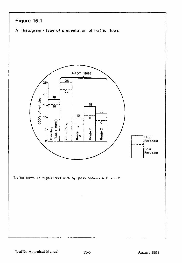
Figure 15.1

A Histogram - type of presentation of traffic flows

AADT 1986

/ *

25

12

-a_ 9

u

3!

z eE:

Traffic flows on High Street with by-pass options A, 8 and C

-. -


1 High Forecast

Low Forecast

August 1991

CHAETER 16 : BEFORE & AFTER MONITORING

16.1 INTRODUCTION

16.2 CATALOGUING THE “BEFORE” PREDICTIONS

16.3 THE “AFTER” COUNTS


CHAPTER 16 : BEFORE & AFTER MONITORING

16.1 INTRODUCTION

16.1.1 The Department operates a system of “Before and After monitoring” which compares the traffic flows resulting from the implementation of a trunk road scheme with those predicted during the scheme’s preparation. To facilitate these

comparisons, EEA division has set up a standard system for recording the forecast traffic flows and for collecting and reporting the traffic counts taken after the scheme has been opened. The aims of this procedure are :-

il to satisfy the demands of good management and public accountability by providing the answers to questions about the effect of a new or improved road;

ii) to identify the strengths and weaknesses in the techniques used for appraising schemes, so that confidence in the roads programme is maintained;

iii) to allow the predictive ability of the models used to be monitored to see whether any particular form of model is consistently more reliable than the others in general use; and

iv) to assist in assessing compensation under Part I of the Land Compensation Act 1973 for depreciation due to the physical factors caused by the use of public works.

The collection of the “after” count information one year after opening is an integral part of scheme preparation and is to be undertaken as a matter of course. The counts are also important in defining the new levels of traffic flow on all links affected by the scheme, and should therefore be incorporated into the National Traffic Count Database held by STC.

16.1.2 The system includes all schemes that are in the National Roads Programme and have reached Order Publication Report Stage since April 1981.


16.2 CATALOGUING THE “BEFORE” PREDICTIONS

L

b

16.2.1 To ensure that the maximum benefit is extracted from the monitoring system, it is essential that the assumptions implicit in the predictions are catalogued in a

uniform manner. This will facilitate the comparisons of traffic forecasts with the after counts for individual schemes and also in assessing the performance of models which may be used in later studies. A standard form TAM 16.1 (reproduced at Figure 16.1) is used for this purpose. The completion of this form is mandatory for the appraisal of trunk road schemes.

16.2.2 For all schemes reaching Order Publication Report stage the procedure for completing the Before form is as follows:-

i) For schemes in the National Roads Programme for which Regional Offices have delegated authority, the Appraisal Certifying Officer is to fill in the form. This is to be sent to EEA when OPR clearance is given.

ii) For schemes which are sent to EEA for endorsement of the economic appraisal the “Before” form will be completed by the appropriate EEA scheme team member. A copy will be sent to Regional Offices for information and comment.

16.2.3 If there are any subsequent changes in the modelling techniques and/or forecasts a revised TAM 16.1 must be produced. However it is expected that the final decision on a scheme will be based on the presentations given at the OPR stage.

16.2.4 When the TAM 16.1 is being prepared EEA will nominate in liaison with the Regional Offices up to four road links affected by the scheme on which “After” counts are to be obtained about one year after opening to traffic (this will include the scheme itself). In reaching the decision as to which roads to include in this exercise, account should be taken of the requirements of public accountability which suggests that traffic flows should be measured where significant changes in flow are anticipated during the assessment of the scheme. Regional Offices may carry out “After” counts at more than just these four locations, if so this information should also be sent to EEA.


16.3 THE “AF-lER” COUNTS

16.3.1 “After” traffic counts, that is counts taken once the improved road has been opened to traffic, may be either:-

i) Counts taken soon after opening, possibly as part of a local “before and after study” to assess the immediate effects of the scheme; or

ii) counts taken in a suitable “neutral” month one year after opening, ie during either April, May, June, September or October.

The first set of counts will provide information about the initial use of the road. The second set of counts will provide long term information and will also provide information useful is assessing compensation under Part I of the Land Compensation Act 1973 for depreciation in the value of interests. in land caused by the use of a new or altered highway. (Part I of the Land Compensation Act 1973, as modified by the Local Government Planning and Land Act 1980, states in Section 4(2) that “In assessing depreciation due to the physical factors caused by the use of any public works, account shall be taken of the use of those works as it exists on the first claim day . ..‘I. The first claim day is the first anniversary of the opening of the scheme to public traffic). Information on the use of new or altered highways may also be of use to District Valuers in the assessment of compensation.

16.3.2 The “After” traffic counts may be either automatic or manual counts and should be undertaken on both new links and those on which major flow changes were expected (suggested links will have been nominated on the Before form). It is recommended that the counts should include 12 hour (7am to 7pm) classified counts where the removal of heavy goods vehicles from a community was a feature of the proposal. The “after” counts taken one year after opening should be as far as possible compatible with the forecast flows.

16.3.3 It is the responsibility of the Regional Offices to collect the “After” counts. The information obtained one year after the opening of the scheme is to be sent to EEA division, on the standard form TAM 16.2 (reproduced at Figure 16.2). As the form seeks the actual count information, it should also be copied directly to STC Division for inclusion in the National Traffic Count Database. For the purposes of “before and after monitoring” it is this information that is required. However there is space on the form for any other counts which may have been taken.

16.3.4 There may be a few schemes for which the traffic counts one year after opening may not fully reflect the effect of the scheme.

i) A scheme may form part of a larger development eg a new motorway. If the traffic model took into account the existence of the other parts of the new road then, and only with the agreement of EEA, the after form can be submitted for counts taken one year “After” the complete development has been open to traffic for one year.


ii) Some roads may have a longer term effect on local traffic patterns than could occur within only one year. However, “after” counts will still be required for the situation one year after opening. Regional off ices may submit to EEA further after forms for later years, if they consider that effects modelled at OPR Stage have been realised at this later time.


APM Division Depanment of Transport 2 Marsham Street London SW1 P 3EB

TAM16.1

APM File ..............................................................

L Telephone 01-212 3162 Contact .................................................................

Before and After monitoring Date . . . . . . . . . . . . . . . . . . . . . . . . . . . . . . . . . . . . . . . . . . . . . . . . . . . . . . . . . . . . . . . . . . . . . .

Record of the “Before” study and Predictions

PartA - General Information

1. (i) Submitting Office:

(ii) Study carried out by:

2. (i) Route number and name of scheme:

(ii) County (if MET County give District or Borough):

3. HMIS Number:

4. Stage of Scheme Preparation Reached (tick one) 0 1. TAR (Technical Appraisal Report) 0 2. Public Consultation q 3. Preferred Route Announcement q 4. OPR (Order Publication Report) 0 5. Public Inquiry 0 6. Works Commitment 0 7. Other (Please specify)

5. Approximate location of scheme (including OSGR):

6. Length of scheme and proposed level of provision:

Classification:- 1. Urban .................................................. .._. km.

2. Rural ....................................................... km.

3. Suburban ....................................................... km.

4. Combination ....................................................... km.

Standard:-

Junctions:-

1. Single 2 lane .......................................... km.

2. Wide single 2 lane ......................................... km.

3. Dual 2/3 lane A/P .......................................... km.

4. Dual 21314 M/Way ......................................... km.

1. Grade Separated

2. Roundabouts

3. Priority junctions

4. Traffic Signals

.......................................... no ..

........................................... no.

........................................ .-no.

.......................................... no.

7. Outline objecti#jes of the scheme:

1. Improvement on existing line

2. Improvement on new alignment

3. Bypass

4. New Route

5. Junction improvement

6. Other (Please specify)

Total Length of Scheme

........................ km.

......................... km.

........................ km.

........................ km.

........................ km.

........................ km.

km.

8. Is the scheme isolated, or part of a larger improvement? (Please specify).


‘APM Use Only

Ref rJo mm Y Y

8 cl

4’url 44 q

August 1991

PartA - Details of the Traffic Model

9. Type of model used (tick one):- 0 1. Link Count only D 2. Junction Count only 0 3. Observed Matrix 0 4. Synthetic Matrix 0 5. Partial Matrix 0 6. Combination of Observed and Synthetic 0 7. Other (Please Specify):-

10. Scale of model: Number of Zones . . . . . . . . . . . . . . . . . . . . .

Number of Links . . . . . . . . . . . . . . . . . . . . .

Matrices Built:- All vehicles only Yes0 Non if no please specify

Private Vehicle Purposes . . . . . . . . . . . . . . . . . . . . . . . . . . . . Commercial Vehicle Purposes . . . . . . . . . . . . . . . . . . . . . . . . . . .

. . . . . . . . . . . . . . . . . . . . . . . . . . . . . . . . . . . . . . . . . . . . . . . . . . . . . . .

. . . . . . . . . . . . . . . . . . . . . . . . . . . . . . . . . . . . . . . . . . . . . . . . . . . . . . .

. . . . . . . . . . . . . . . . . . . . . . . . . . . . . . . . . . . . . . . . . . . . . . . . . . . . . . .

. . . . . . . . . . . . . . . . . . . . . . . . . . . . . . . . . . . . . . . . . . . . . . . . . . . . . . .

11. Model database.

1.

2.

3.

4.

5.

6.

7.

8.

9.

Household Interviews

Roadside Interviews

Manual Classifieo Counts

Automatic Traffic Counts

Junction Counts

Link count only

Reg No Survey

Commercial vehicle survey

Other (Please Specify):-

Date Date Date

.................... .................... .....................

.................... ................... .....................

.................... ................... .....................

.................... ................... .....................

.................... ................... .....................

.................... ................... .....................

.................... ................... .....................

.................... ................... .....................

.................... ................... .....................

12. Base of model: Hours . . . . . . . . . . Days . . . . . . . . . . . . . . . . Month . . . . . . . . . . . . . . . Year . . . . .._.........

Vehicle types modelled: Cars/LGV/OGVl/OGV2/MC/PSV (delete as appropriate)

13. Present Year Validation: Yes Cl Non if Yes state Year . . . . . . . . . . . . . . . . . . . . . . . . . . . . . . . . . .

14. Details of any sub-models used:

Computer Suite Used . . . . . . . . . . . . . . . . . . . . . . . . . . . . . . . . . . . . . . . . . . . . . . . . . . .._........................

Car Ownership model - YesO Nom

Trip End Model - YesO Noa

Trip Distribution Model- Yeso Non

Assignment Model - Yes 17 Nonif yes please specify:-

1. All vehicle

Was any fitting of route choice parameters undertaken? Yes 0 Nom

45-7

““CcIrl ““17

54 q 55

PV iI 56

cv q

hhdmmvy

‘2) J J J J J J

“ll


15. Was modal competition assessed?

If yes please specify:-

Yes 0 No 0

16. Details of network speed coding

El 1.

x f : b 4. Cl 5.

(please tick relevant coding):- LF 170 Advice Note 1A COBA Curves Observed Journey Times Other (Please Specify): -

17. Were the conversion factors used to convert survey data to the traffic model base derived from (please tick): 0 1. Local Data

0 2. National Data 0 3. Combination of local and national data

Part B - The Forecasting Process

18. Predicted year of opening: ........................................................................................................

Year(s) for which traffic forecasts have been produced .............................................................

19. Are network changes assumed between the base year and forecast years?

(in addition to the scheme studied): Yes 0 No 0

If yes please list schemes:-

43rl

Traffic Appraisal Manual 16-9 August. 1991

20. Derivation of forecast land use planning or trip end data used: (eg National Planning Data Files (PD86D), National Trip End Files (TAB 86D))

1. From National Trip End Data Files?


Yes Cl

2. From National Planning Data Files?


Yes Cl

3. From Local Planning Data? If yes please specify:-

Yes Cl

4. Were any major developments considered separately? YesO If yes please specify:-

21. National Forecasts used and how control was applied:

Vehicle Type

1. Private Vehicles

2. Commercial Vehicles

Section of Matrh eg External/ Internal, All

Uational Forecasl !g NRTF and JFAF. No :ontrol

Stage at which :ontrol applied eg Trip Ends, Matrix Totals

Level at which control applied eg District,

County, Matrix total

The’ Results of the Traffic Appraisal

22. Please attach a schematic diagram of the scheme study area showing the base year and the do- minimum and do-something range of predicted traffic flows in the forecast years for the preferred route and those roads which receive substantial relief. (Maximum size A3). Please state traffic flow units.

52 q

53 q

54 cl

55

n

56177

.- ‘I 31

flow (000’S)

2 std year low - high

link A I

Link: m

16 ~IinkC ! I1 -


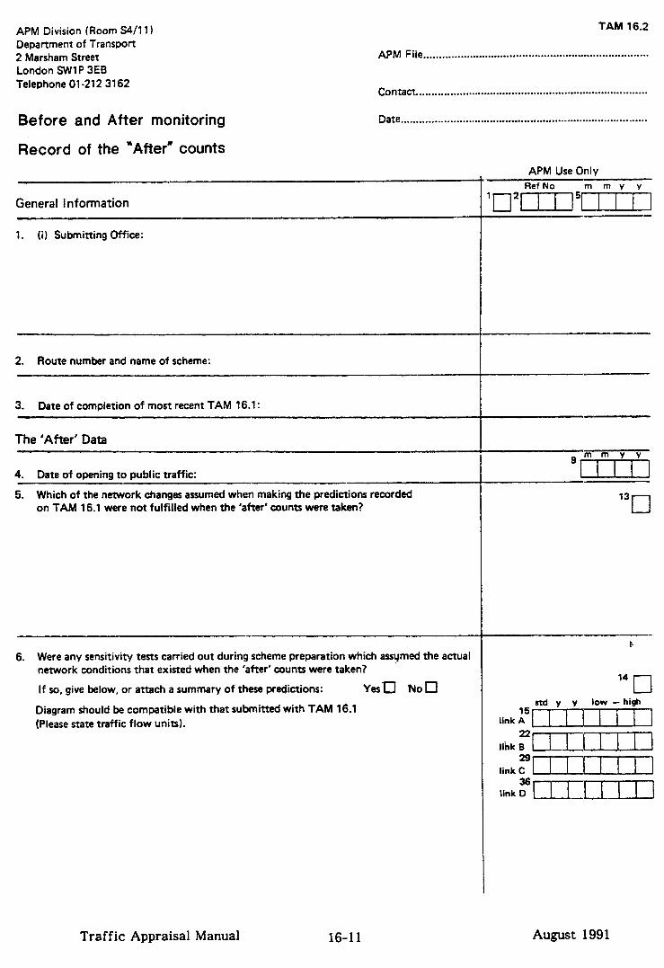
APM Division (Room M/l 1) Department of Transport 2 Marsham Street London SW1 P 3E6 Telephone 01-212 3162

Before and After monitoring

Record of the “After” counts

TAM 16.2

APM File . . . . . . . . . . . . . . . . . . . . . . . . . . . . . . . . . . . . . . . . . . . . . . . . . . . . . . . . . . . . . . . . . . . . . . . . .

Contact ...........................................................................

Date ................................................................................

I APM Use Only

I Ref No m my Y

General Information

1. (i) Submitting Office:

‘n2KII15uul

2. Route number and name of scheme: Ll

3. Date of completion of most recent TAM 16.1:

The ‘After’ Data

5. Which of the network changes assumed when making the predictions recor on TAM 16.1 were not fulfilled when the ‘after’ counts were taken?

L

6. Were any sensitivity tests carried out during scheme preparation which assumed the actual network conditions that existed when the ‘after’ counts were taken?

If so, give below, or attach a summary of these predictions: Yesa No0

Diagram should be compatible with that submitted with TAM 16.1

(Please state traffic flow units).

Traffic Appraisal Manual 16-1 I August 1991

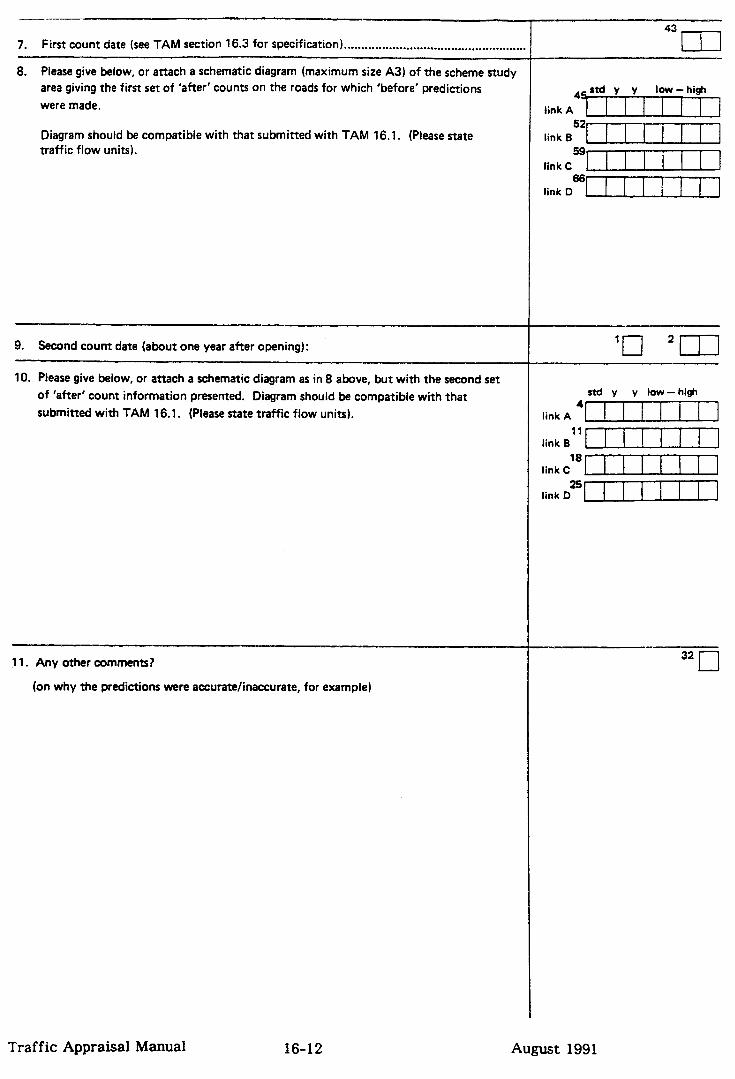
7. First count date (see TAM section 16.3 for specification) . ..-................................................

8. Please give below, or attach a schematic diagram (maximum size A3) of the scheme study

area giving the first set of ‘after’ counts on the roads for which ‘before’ predictions

were made.

Diagram should be compatible with that submitted with TAM 16.1. (Please state

traffic flow units).

10.

9. Second count date (about one year after opening):

Please give below, or attach a schematic diagram as in 8 above, but with the second set

of ‘after’ count information presented. Diagram should be compatible with that

submitted with TAM 16.1. (Please state traffic flow units).

Il. Any other comments?

(on why the predictions were accurate/inaccurate, for example)

43ll I 1 I

link A

link B “‘I

link C ““I-l_r

link D “I

std Y y low-high

link A *EIIlImn

link B “m

link C ‘“II

““I link D

32 q


czH2wmR 17 : ESTIMATING TRAF'FIC UNDER MODAL COMPETITION

17.1 GENERAL

17.2 APPRAISING COMPETITION FROM OTHER MODES

17.3 SIMPLE TECHNIQUES FOR THE ASSESSMENT OF MODAL SPLIT

17.4 MORE COMPLEX MODAL SPLIT MODELS

17.5 LIAISON WITH OFFICERS FROM OTHER TRANSPORT AUTHORITIES



c!mPTEx 17 : ESTIMATING TEtAF'FIC UNDER MODAL COMPETITION

17.1 GENERAL

17.1.1 This chapter deals with the procedures and techniques for assessing the effects of modal competition where they are relevant.

Section 17.1 sets out the findings of The Standing Advisory Committee on Trunk Road Assessment (SACTRA), before describing the procedures to be followed to deal with the modal split question.

Section 17.2 discusses the issues related to the estimation of modal split.

Section 17.3 deals with simple techniques for the assessment of modal split.

Annendix 17 describes simple methods for the estimation of modal split and changes in modal split. It contains formats for work-sheets and a set of curves of modal split vs. difference in travel impedances between public and private transport; and changes in modal split due to changes in difference in travel impedances between public and private transport.

Section 17.4 discusses some of the issues related to conventional multi-stage transport models that include a modal split phase and

Section 17.5 discusses procedures for liaising with officers from other transport authorities. Finally,

Annendix 17.2 discusses the problems associated with the development of the simple technique for the assessment of modal split and gives an indication of the limitations of the method.

17.1.2 SACTRA reported that “The proportion of journeys by public transport varies greatly. in particular it is heavily used for journeys in major inter-urban corridors and for journeys to work within conurbations. For example, . ..“. (SACTRA 8.32).

17.1.3 They concluded that “It is essential that an adequate representation of the base year flows be obtained before making a judgement on those circumstances in which a multi-modal approach to forecasting will be appropriate. For this reason we think that it would be unwise for any future models to assume that modal share considerations are irrelevant to traffic forecasts for particular schemes without thorough investigation. Nevertheless, we believe that there will be many cases where a single-mode approach to forecasting will, in practice, be adequate”. (SACTRA 8.341.

17.1.4 The Department accepts the conclusions in principle. In the appraisal of many, if not most, trunk road schemes, a single-mode approach will be adequate.


Very occasionally, and only when the planning brief requires it, should an examination of modal competition be undertaken. The recommended procedures to be followed are shown on Fig 17.1 with which the following description should be read.

17.1.5 If the planning brief does not require an examination of modal competition or if commonsense and judgement indicate that no work on modal split should be done because the scheme is so minor and/or remote from competitive public transport facilities, then a reasoned statement should be prepared for traffic appraisal reports. This should set out the likely effects of the scheme, and give a short inventory of public transport facilities available in the vicinity of the scheme. This procedure is also to be followed if the public transport operator does not believe that the scheme will have an appreciable impact on his operations.

17.1.6 If the public transport operator considers that the scheme is likely to have a significant impact on his operations but has no firm new proposals of his own likely to compete for trunk road traffic, then he should be requested to produce estimates of revenue loss or gain. The Department will then have to discuss and reach agreement on the estimates produced by the operator. If agreement is reached then a statement should be prepared for traffic appraisal reports and no further work on modal split would be required.

17.1.7 If the public transport operator has firm new proposals or is unable to provide estimates of revenue loss or gain of his operations then the implications of the road proposal and public transport operations will have to be examined.

17.1.8 If existing recent local transportation study data or national census data are available on mode shares and are adequate to derive information for assessments on likely revenue changes, public transport usage, etc then no further work would be required on modal split for the preparation of a statement for traffic appraisal reports.

17.1.9 If no suitable data on modal split are available, but if the scheme is not too large nor part of a complex network and therefore lends itself to appraisal by simple techniques, then the method described in Appendix 17.1(l) can be used to assess the modal split. If the estimate of modal split is adequate to derive information for assessments on likely public transport revenue change, public transport usage, etc then no further work would be required on modal split for the preparation of a statement for traffic appraisal reports.

17.1.10 If the estimate of existing modal split from existing data sources or the use of a simple technique is not adequate to derive information for assessments, but if the scheme is of suitable size and nature (see 17.1.9) then the change in modal shares may be assessed by using the simple technique described in appendix 17.1(5). If the estimate of change in mode shares is adequate to derive information for assessments, then no further work would be required on modal split for the preparation of a statement for traffic appraisal reports.

17.1.11 If no suitable data on modal split are available or if the scheme cannot be assessed by the use of a simple technique, then EEA Division in HQ should be contacted about the need for complex mode split modelling.


( 1 Q

Is the scheme so minor andj?or remote from public transpor! alternatives that commonsense and judgement say that no work should be done on modal split?

a 1

Does the public transport operator belleve that the scheme will have an appreciable impact on his operations 7

NO\ \

\t

YES

/’

Prepare a reasoned statement in traffic appraisal reports setting out the likely effects of the scheme

transport alternatives

t YES

NO 1

1 bar lpro

on : salsj

i

NO

Does existing census data or local transportation study data give adequate information on share of travel by mode?

I

t

YES

-E

Is it adequate to derive information for decisions e. estimates 0 8’ revenue change use ot public transport bv

-2

FLOW-CHART OF PROCEDURES FOR THE ASSESSMENT OF MODAL SPLIT

FIG. 17*1

to proposals be

estimated by

17.2 APPRAISING COMPETITION FROM OTHER MODES

17.2.1 The measure of competitiveness between modes for passenger transport has been generally assessed in past urban transportation studies by an analysis of the following factors:-

i) the characteristics of the trip eg length, purpose, time of day;

ii) the characteristics of the traveller eg socio-economic group, car ownership;

iii) the characteristics of the transportation system eg accessibility, travel time, travel cost, comfort and convenience.

The choice of a particular mode is influenced by a combination of several factors such as the availability and reliability of travel modes, journey length, speed and cost; socio-economic traits of the traveller and comfort and convenience of travel. Some of these factors such as convenience are difficult to quantify and are treated as having little influence on mode choice or are incorporated as proxies with other more readily quantifiable parameters such as waiting and transfer time for public transport.

17.22 National census and local study (eg West Yorkshire, Bristol, GLTS) data sources indicate that although the total number of long distance trips is proportionately small, rail plays a more than marginal role in this field and its relative importance increases with increasing trip length. Rail’s share of journeys made between individual origins and individual destinations varies considerably. It is particularly important in London for both commuting and for long distance business trips. The radial nature of rail in the cities is a contributory factor to the use of rail for travel to city centres, particularly for journeys to work. National long distance coach trips are naturally weighted towards longer distances and 50% of such trips are over 25 miles in length.

17.2.3 Peak trips within built-up areas are largely work trips of short lengths, whilst inter-urban trips tend to be long and for a mix of purposes. Public transport is a major competitor with private transport in and around the conurbations. In the majority of inter-urban cases the effect of competition from other modes may not be significant in terms of estimating traffic volumes on trunk roads. However, there may be instances where the existence of parallel facilities as viable alternatives to private transport necessitate the consideration of modal competition. This has been recognised in a number of past studies that have used multi-mode transport models to cope with modal choice. The decisions whether to model modal choice or not has to be taken by a consideration of the relevant factors in each case. If it is decided that modal split should be modelled, ‘then the choice of model would be dictated by the nature and location of the scheme.


17.2.4 In the estimation of trunk road traffic, consideration will have to be given to the competition to private transport from bus, rail and long distance coaches. It is, however, unlikely that air and water transport would provide viable alternatives to road transport except in a few special cases which are not relevant to the current road construction programme.

17.2.5 The characteristics of freight traffic are different from those of passenger traffic. Passenger behaviour is closely related to the cost and quality of transport services. This is not true of freight traffic where the direct cost of transport usually only comprises a small proportion of the total cost of a commodity. British and continental studies (eg ref l-3) have shown that reliability and speed play a greater part than cost in the mode choice decisions for freight.


17.3 SIMPLE TECHNIQUES FOR THE ASSESSMENT OF MODAL SPLIT

17.3.1 If the scheme is not too large and is located where its effects are unlikely to spread over a wide area of the network, then the modal competition between the scheme and existing or proposed public transport facilities near the scheme may be assessed using the technique described in Appendix 17.1, or some other similar method.


17.4 MORE COMPLEX MODAL SPLIT MODELS

17.4.1 If a scheme is located in an area where extensive public transport facilities exist and its effects are likely to spread over a wide area of the network, then it may require a more sophisticated approach to the modelling of mode-choice. This is likely to involve the building of a public transport network along with the highway network for the study area, and a modal split phase in a conventional transport model. The choice of approach to modelling modal split must relate to the decisions to be taken and be tailored to the availability and quality of data and the availability of an appropriate model. Current practice is largely dependent on the existence and availability of local models. This is understandable, as the additional accuracy that can be achieved by developing a model for a specific application may not justify the effort in time and money associated with model development. If a preliminary examination of census or other survey data, or the use of a simple modal split model indicates a complex modelling approach, EEA Division in HQ should be consulted before any detailed work is undertaken.

Annroaches to Mode Choice Modelling

17.4.2 Figure 17.2 illustrates the different stages of the conventional comprehensive transport model. Modal split can be introduced at different points in the modelling process, which is a reflection of the interactive nature of mode choice decisions. Modal split can be considered:

i) at the trip generation stage,

ii) after generation and before distribution,

iii) as part of distribution,

iv) after distribution.

The factors which can be taken into account and the method of doing so are largely determined by the stage at which the calculation is introduced. In past studies, at the generation phase factors such as household income and composition and car ownership have been included in regression analysis or category analysis. Households have been classified into car-owning and non-car-owning to approximate the effect of mode availability. It has been assumed that the majority of trips by non-car- owning households are captive to public transport. Trips by car-owning households have been split into private and public transport trip ends by means of zonal accessibility indices included either in the regression equations or as an additional category for category analysis. With modal split after generation and before distribution, the total trip ends by all modes for each purpose are split into the proportions using the different modes by multiple regression analysis. The dependent variables would be proportion of home-based work trips by car, proportion of home- based other trips by car, etc. The independent variables would be similar to those in the previous case and would not include trip characteristics such as length, travel cost, etc.

Traffic Appraisal Manual 17-9 August 199i

When modal split is part of the distribution phase or is after distribution, generation factors (eg purpose, mode availability) as well as journey characteristics (eg length, cost) are taken into account. These models allocate proportions of given trip movements to alternative modes by regression techniques and more usually by the use of ‘diversion curves’ in the case of post-distribution modal split models.

17.4.3 There are no overwhelming reasons for selecting a particular modelling procedure a priori, and decisions on model adequacy and sophistication must be based on information acquired through observation. Little information is readily available about the performance of modal split models used in past studies. Model validation is, however, an essential part of the modelling process and efforts should, therefore, be made to determine how well the model performs against observed data.


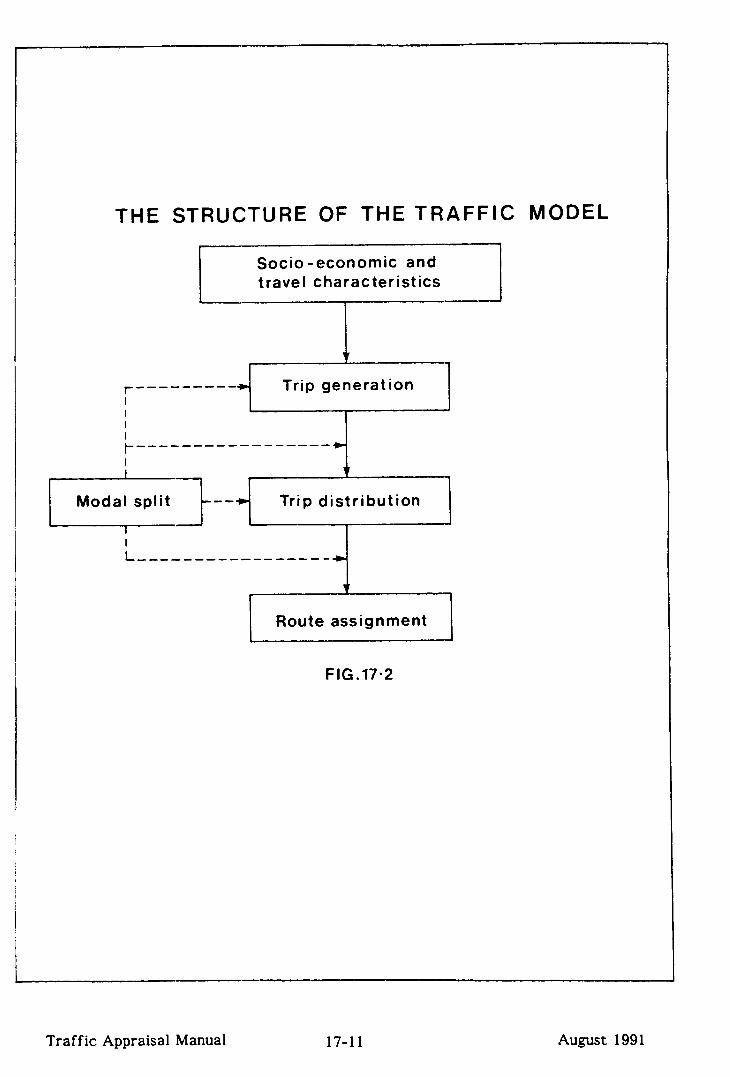
THE STRUCTURE OF THE TRAFFIC

_-----a-- Trip generat ion

I I

~______--_--------

rip distribution

I Route assignment I

FIG .17-Z

MODEL


17.5 LIAISON WITH OFFICERS FROM OTHER TRANSPORT AUTHORITIES

17.5.1 Modal choice decisions are often influenced by changes to the transportation system. Prior knowledge of such changes would enable proper decisions being taken about the manner of handling mode-choice. It is therefore necessary to develop and maintain channels of communication with other transport authorities so that exchange of information on proposed changes to transportation systems can be of mutual benefit and promote co-ordinated planning effort. 1

17.52 If it is considered that a proposed scheme is in competition with an alternative mode, then the relevant public transport authority has to be consulted. Rail and bus services are provided by British Rail (BR), National Bus Company (NBC) subsidiaries, private and/or municipal undertakings. However, where local authorities provide financial support, local service levels are influenced by the Metropolitan County Councils in conjunction with the Passenger Transport Executives (PTE) in metropolitan counties, and by the County Councils in shire counties. In London, most bus and all underground services are operated by London Regional Transport (LRT) whilst BR are responsible for rail services. Initially, therefore, the PTE, County Council or LTE has to be approached and through it the operator concerned, be it the NBC subsidiary, private or municipal operator or BR Region. If matters cannot be resolved at a local level particularly with regard to rail services then EEA Division should be contacted for liaison with BR HQ through the appropriate HQ Directorate.

17.5.3 When alternative transport solutions to a trunk road scheme involve public transport modes then their operational feasibility and financial viability have to be considered. In such cases the capital and revenue costs, staff and service levels, and routes and schedules, besides the travel demand and mode share, have to be worked out in conjunction with the appropriate public transport authority. Every attempt must be made to arrive at agreed figures.


REFERJSCES - CHAPTER 17

1. Bayliss B T & Edwards S L: “Industrial Demand for Transport”, HMSO, 1970.

2. “Review of the Commodity Flow Studies (1975-79)“, extracts from research report no 36, University of Newcastle-upon-Tyne.

3. Chisholm M & O’Sullivan P: “Freight Flows and Spatial Aspects of the British Economy”, Cambridge University Press, 1973.


CHAPTER 18 : APPRAISING TRUNK ROAD SCHEMES INURBANAREAS

18.1 GENERAL

18.2 THE COMPREHENSIVE APPROACH

18.3 URBAN TRAFFIC ENGINEERING TECHNIQUES

18.4 TRAFFIC MANAGEMENT AND APPRAISAL IN URBAN AREAS



CHApTER 18 : APPRAISING TRUNK INURRANAREAS

ROAD SCHEMES

18.1 GENERAL

18.1.1 Some of the most difficult appraisal problems are found close to and in urban areas, and the framework approach for the assessment of trunk road schemes has a heredity which can be traced to this source. The importance of elements in the framework which are difficult or impossible to quantify in monetary terms is even greater in the typical urban and peri-urban scheme then in its general rural counterpart. The information provided by the traffic appraisal should reflect the complexity of the situation, striking a balance between the need to model elements of the transport system in a realistic way, and the objective of providing only sufficient information for good decisions to be made, and no more.

18.1.2 Analytical techniques which work reliably in rural areas may not be valid for urban traffic appraisal, and a variety of techniques have been developed for use in the urban setting. The choice of techniques appropriate to a particular urban scheme should be a matter for local judgement and responsibility. Before adopting more complex methods, the short-comings of the simplest techniques should be fully explored, to provide the justification for adopting more sophisticated and extensive methods. While there are cases where comprehensive transport models will be required, or the interaction between the transport system and land use must be taken into account, these options should only be considered when it is clear that simpler approaches would give misleading results.

18.1.3 This manual is primarily concerned with the appraisal of trunk road schemes, but this chapter contains some discussion of the wider transport planning principles which are, for the most part, the province of other transport authorities. The need for liaison with these authorities is emphasised, but it must be remembered that they will have different objectives, and while there should be no conflict of objectives, they will have a wider remit than those carrying out the traffic appraisal.


18.2 THE COMPRJZHENSI’IE APPROACH

L,-

L

18.2.1 The traffic engineer appraising a road scheme in or near an urban area cannot be concerned solely with moving general traffic faster. Whilst this objective is valid in most cases, it can conflict with other objectives concerning, for example, public transport or the attractiveness of a busy shopping street. No network of roads is without traffic management, even if only by default. In recent years the sum of individual traffic management measures has been recognised to have an effect much greater than its component parts, and planning frameworks known as “Comprehensive Traffic Management” (UK) or “Transport Systems Management” (US) have evolved to allow the design of urban transport in a structured way. Within Comprehensive Traffic Management (CTM), road building has to be considered for its overall place and contribution because CTM can take place with or without a new road as a component part. Figure 18.1 and Figure 18.2 are idealised flow charts of the CTM approach and the working out of CTM options respectively.

18.2.2 An important principle of CTM is that traffic must be understood as a derived demand for the movement of people and goods, not just as road vehicles. The approach to movement in CTM passes through three stages as the demand for road space exceeds supply: this is closely correlated to city size (see Figure 18.3). These stages are:

i) Manage for canacitv: traffic management (including construction) can be applied to keep all traffic moving;

ii) Manage for nriority: there is inadequate capacity for general traffic, but priority measures can be taken to redistribute delays to benefit selected types of movement; and

iii) Manage demaa: action can be taken to deter or remove traffic from the road network. (Parking control is generally the most effective measure).

18.2.3 The component tools of CTM are summarised in Table 18.1. (An important difference between construction and management measures is that the latter are generally reversible and can be applied using experimental orders in the first instance: in practice, many experimental orders are modified or rescinded).

18.2.4 A standard procedure in the design of traffic management schemes is to distinguish between 3 types of traffic:

i) through traffic (external-external);

ii) internal traffic (internal-internal); and

iii) terminal traffic (external-internal, internal-external)

and to attempt to identify the function which roads in the urban network should perform ie:


i) primary distributors;

ii) district distributors; and

iii) local distributors.

Trunk roads are generally identified as having the function of primary distributors carrying through traffic: they will also serve, perhaps even dominantly in terms of vehicle numbers, lower level functions as well.

TABLE 18.1

Components of Comprehensive Traffic Management

Turning Restrictions One-Way Streets

Construction

Traffic Route Signing

Bus Priority at Signals Pedestrianisation

Street Parking Control

Junction Design

Partial Closure of Urban Traffic Control


CTM OPTIONS

2. GOALS ACHIEVED

IMPLEMENT

EXTERNALITIES

PROCESS STEPS

AN APPROACH TO DESIGN FOR COMPREHENSIVE TRAFFIC MANAGEMENT

FIG.18.1


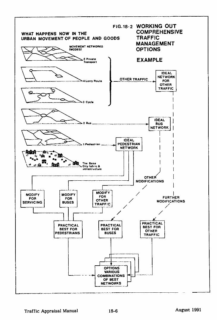
FIG.18.2 WORKING OUT WHAT HAPPENS NOW IN THE COMPREHENSIVE URBAN MOVEMENT OF PEOPLE AND GOODS TRAFFIC

NT NETWORKS

5 Private Transport

MANAGEMENT OPTIONS

EXAMPLE

OTHER TRAFFIC

2 Bus BUS

1 Pedestrian

The Base City fabric & mfrastructurc

MODIFY FOR

SERVICING

I I

I OTHER

MODIFICATIONS / I / I / I

/ FURTHER

MODIFICATIONS

/ /


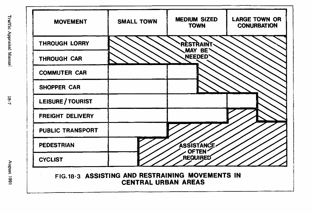
I I I I SMALL TOWN MEDIUM SIZED LARG

TOWN COI munurv UVII

iE TOWN OR UI IDDAIInN

MOVEMENT

THROUGH LORRY

THROUGH CAR

COMMUTER CAR

FIG.1&3 ASSISTING AND RESTRAINING MOVEMENTS IN CENTRALURBAN AREAS

18.25 The Departmental objectives (which will usually concern more than just the urban area) and those of Local Authorities (county and district) will need to be considered in the design of a successful urban and inter-urban transport system. In most cases these objectives will be shared; for example, the provision of a trunk road by-pass which removes through traffic may be the key to a CTM scheme including pedestrianisation of the High Street and much else. There will be rare but perhaps unavoidable occasions where the role of the trunk road as seen by the Department will conflict with the local view of transportation priorities. The conflict may arise because of different judgements on environmental impact or other benefits; or because the provision of increased road capacity is incompatible with local authority traffic restraint policies.

18.2.6 The position of some inner cities can be particularly difficult in this respect. The Local Authorities responsible for these areas can often point to their low car ownership and heavy reliance on public transport: traffic problems in their view are caused by commuter traffic from more prosperous suburbs travelling through the inner city to the central business district. The management policy of these authorities is often carefully thought out and determined as they seek to channel through traffic away from residential areas on to primary distributors on which they have provided extensive bus priorities (bus lanes, priority turns, selective detection at signals and so on).

18.2.7 Attention should therefore be paid to the interface of trunk roads with the Local Authority network and the associated management required to make a trunk road scheme work. This should be done, if possible as a joint exercise with the Local Authority, once options that are otherwise feasible have been developed.

18.2.8 In some cases, trunk road objectives may be met by CTM alone. A CTM scheme, with the associated low costs, can give a very high rate of return. CTM schemes are difficult to design and can require considerable planning. In addition, the distribution of their costs and benefits are likely to be different in many respects from a construction alternative.

18.2.9 Further, the construction alternatives considered should not solely be restricted to general all-purpose roads: for example, segregation of buses, cycles or commercial vehicles on to separate tracks or the completion of a one-way system with a new link might be considered (Figures 18.4-7 illustrate three alternative approaches for construction).


FIG. 18.4

AN EXISTING

NETWORK

FIG. 18.5

THE TRADITIONAL MAJOR

CON STRUCTION SCHEME

IdAY 1981


FIG.18.6

A CUT PRICE CONSTRUCTION ALTERNATIVE

FIG. 18.7

A COST EFFECTIVE AND BALANCED CONSTRUCTION ALTERNATIVE


18.3 UREUW TRAFFIC ENG INEERING TECHNIQUES

18.3.1 The analytical tools and techniques involved are not wholly unique to urban areas, and are described in chapter 13.

18.3.2 References 1 to 14 are relevant publications concerning the implementation of urban traffic engineering measures. Attention is particularly to be drawn to reference 2 which contains references to publications which supersede particular sections of the 1966 publication “Roads to Urban Areas” (ref 1). The Institute of Highways and Transportation is currently undertaking a study of design standards and procedures for roads in urban areas (to be completed in 1985).


18.4 TFtAFFIC MANAGINENT AND APPRAISAL lNuFu3ANAREAs

18.4.1 This section discusses some of the more difficult areas of traffic and economic appraisal where traffic management is involved.

18.4.2 The appraisal of schemes can be considered in three categories (as in section 18.2):

i) appraisals concerned only with capacity;

ii) appraisals concerned with priority (but not demand management); and

iii) appraisals concerned with demand management.

18.4.3 Those undertaking appraisal of trunk road schemes should always consider the “do minimum” condition carefully. The local authority proposals for traffic management (as in the case of construction) can often affect the rate of return of a trunk road scheme substantially. Traffic management may indeed be an alternative option.

18.4.4 Considerable thought should however be given to the requirements of the appraisal. What is done should be relevant to the problem under consideration. If the scheme is a localised traffic management improvement where fine tuning is required then detailed calculations, perhaps including the number of vehicle stops and starts, may be required and a single year rate of return may be appropriate. The analysis of most major urban trunk road schemes will require the COBA approach as used in all major trunk road schemes. Advice on economic appraisals in urban areas falling outside situations described in Chapter 14 and covered in the COBA manual should be freely sought from EEA scheme teams.

18.4.5 The appraisals in this category are the main stream of trunk road work. However, the use of speed-flow curves alone (which incorporates some allowance for junction delays) may well prove inadequate where some junctions are expected to operate either close to or over capacity; or to interact one with another (see also 13.5).

Annraisals Concerned with priority

18.4.6 Where schemes are being appraised which involve priority, estimates of time savings and losses, and operating costs of the different threads of movement (cars, cyclists, buses, commercial vehicles, pedestrians) should be undertaken as appropriate. Appraisals will usually be undertaken for peak and off-peak periods and an economic rate of return based on one year calculated: for more strategic schemes, a future year return should be calculated as well and benefits interpolated and discounted over thirty years.


184.7 Where buses are involved and the objective of a scheme (perhaps a public transport alternative) is aimed at achieving more economical schedules for a given pattern of service, or more extensive service without increase of fleet, then a different approach may be required. Rescheduling cannot be done to save only part of a bus, and there are many constraints arising from the nature of bus operation (crew roistering, passenger requirements and so on). In the case of tactical schemes which are well developed then it may be appropriate to switch from the usual average benefits method (embraced by the “value of time” approach) to a micro- economic analysis agreed with the public transport authority (see also 17.5). (Ref 15) contains an appraisal of the average benefits type; (ref 16) “Bus Selective Detection in Swansea’ covers an appraisal of the micro-economic type.

ADDraidS under Demand Management

184.8 Appraisals under demand management will be very rare.

184.9 Economic appraisals undertaken by the Department are of the consumer surplus type (see COBA manual). In application there is an important distinction between an elastic and inelastic demand for travel with respect to cost of travel. An inelastic demand (as in COBA) allows the simple difference in user costs between an economic base and an alternative to represent benefits. An elastic demand requires both a model to estimate changed travel demand and a different analytical method to allow computation of benefit.

18.4.10 Most elastic travel demand models are of the gravity type, concerned solely with redistribution (change of origin or destination) and additionally in major models with simple change of mode, not with the full range of options in practice adopted by travellers. This is not surprising as there is no body of theory, practice or supporting data base to model the more complex interactions that can occur in practice over the urban area. For example:

Pure restraint: “I will watch television rather than go to the cinema now that I have to park five minutes walk away”.

Reassignment in time: “If I get up earlier than I would like, I can drive in before the rush hour starts. It takes me twenty minutes then: it takes me forty in the rush hour.

I would like to go in the rush hour if it took me thirty minutes as it did before they closed off my little back route”.

Reliability: “I go by the by-pass rather than the town centre. On average it’s quicker through the centre but sometimes I get held up and get into work very late”.


Transferabilitv: “Darling, will you pick up a loaf of bread on your way home. They have put double yellow lines outside the ‘Golden Loaf”‘.

Consolidation: “I decided to get that new washing up bowl when I went to the library today rather than go out tomorrow. I could not face that trip in again with that stupid one-way system”.

Comnlex Mode Cho& “Mr Jones next door used to drop me off at the bridge where I could pick up the bus. Now with the cycle route through the park, on Tuesday and Friday I dump my bike at Aunty Joan’s when her friend Harry can drive me in”.

18.4.11 A model structure has been proposed by Robertson and Kennedy (ref 17) and two household based procedures which consider these more complex interactions

- -i - caiied HATS (Househoid Activity Travel Slmuiatorj and CARLA (Combinatorial Algorithm for Rescheduling Lists of Activities) - have been developed by Oxford Transport Studies Unit (refs 18 and 19). Some of these interactions are satisfactorily described at macro-level by redistribution models and small scale use of techniques such as HATS can provide qualitative information as well as giving guidance on appropriate survey and modelling techniques. There is however no parallel accepted economic procedure which has been developed which embraces all effects.

18.4.12 Some of the detailed effects of demand management are likely to be so uncertainly estimated (and expensive to estimate) that their overall impact is best considered within the context of the framework. If the condition arises that user benefits are being achieved at the expense of suppressed trips then the framework must make this quite clear.

18.4.13 EEA should always be consulted in the case of economic evaluation of restraint schemes.


L

t

REFJSENCES - CHApllER 18

(Note: This is not a complete list of relevant Departmental Publications. A full list of technical memoranda, departmental standards, advice notes and circular roads is available from Room P3/030, 2 Marsham Street, London SWl).

1.

2.

3.

4.

5.

6.

7.

8.

9.

10.

11.

12.

13.

14.

“Roads in Urban Areas”, Ministry of Transport, Scottish Development Department, The Welsh Office, HMSO, 1966.

“Roads in Urban Areas, Supplement, A Guide to Revisions 1979”, Department of Transport, Scottish Development Department, The Welsh Office, HMSO, 1979.

Webster F V and Cobbe B M, “Traffic Signals”, Road Research Technical Paper No 56, TRRL, 1966.

Robertson D I, “TRANSYT: a traffic network study tool”, TRRL, LR253, 1969.

Vincent R A, Mitchell A I, Robertson D I, “User guide to TRANSYT version 8”, TRRL, LR888, 1980.

I ecnnicai Memorandum Hi/73 - “Criteria for traffic light signals at junctions”.

Technical Memorandum Hl l/76 - “The design of major/minor priority junctions”.

Technical Memorandum HZ/75 - “The design of major/minor priority junctions”. iSee aiso TE design Note i j.

Technical Memorandum H6/76 - “Implementation of bus priorities”.

Technical Memorandum HZ/77 - “Bus Priority at Traffic Signals Using c~‘~.+;..~ na+a-+:rr-n &nzI’z~CI.‘z u=L=L’.L”‘I .

Circular Roads 42/73 - “Pedestrian Safety” Manual.

Circular Roads 8/78 - “Conversion of Normal Roundabout to Mini or Midi Roundabout”.

“-r,,rc:, ,l--r-----L --_a ~--l-f_-” x,f-:-&-_ -c CT----- __ “LI~JAL IVAS~II~~AII~;IIL iiuu rar-KIII~ , NIIIIISU~ 01 I ransport, ‘Welsh Office; Department of Transport, Room P1/097, 2 Marsham Street, London SWl.

“Ways of Helping Cyclists in Built-Up Areas”, Department of Transport, Welsh Office; Local Transport Note l/78; Department of Transport, Room P1/046, 2 Marsham Street, London SW1


15. Cooper B R, Vincent R A and Wood K, “Bus-actuated traffic signals - initial assessment of part of the Swansea bus priority scheme”. TRRL, LR925, 1980.

16. “Bus Selective Detection in Swansea”, Traffic Advisory Unit, Department of Transport, Room P1/085, 2 Marsham Street, London SWl.

17. Robertson D I and Kennedy J V, “The Choice of route, mode, origin and destination by calculation and simulation”, TRRL, LR877, 1979.

18. Jones P M, Dix M C, Clarke M I, Heggie I G, “Understanding Travel Behaviour”, Report 119/PR, 1980, Transport Studies Unit, Oxford University.

19. Clarke M I and Dix M C, “An Activity Scheduling Model for Generating Feasible Travel Choice Sets”, Report 129/CP, 1980, Transport Studies Unit, Oxford University.


CHAPTER19 :THEAPPRAISALOFSMALLER

TRUNK ROAD SCHEMES

19.1 DEFINITION OF A SMALLER SCHEME

19.2 THE APPRAISAL OF SMALL SCHEMES


c

cHAP!rER 19 : !rHE APPRAISAL OF SMALLER TRUNK ROAD SCHEMES

19.1 DEFINITION OF A SMALLER SCHEME

19.1.1 The effects of a highway scheme depend on its size and location. Large schemes, naturally, produce greater impacts on their surroundings than do smaller ones in similar locations. On the other hand, if the scheme is an integral part of a complex network in a built up area, its effects will be greater than a scheme of comparable size in a rural setting. Because the scale of effects vary with scheme size and location, different assessment methods are used to evaluate them.

19.1.2 A small scheme is defined for this purpose as one with a total cost (works and land) of less than El,OOO,OOO. Schemes costing over UOO,OOO require individual assessments. The results of assessments of schemes costing over &ZOO,000 are recorded on Form 502. The current version of Form 502 is compatible with TAM procedures and has also been updated in line with the NRTF and the latest GDP forecasts. Schemes costing between ElOO,OOO and ;E200,000 are not subject to such formal assessments but the methods used should be consistent with the general approach applied to the more expensive schemes, perhaps by using simpler methods. Schemes costing over e500,OOO require approval by FH division.


19.2 THE APPRAISAL OF SMALL SCHEMES

19.2.1 The need for most schemes is indicated by deficiencies in one or more of three basic elements: traffic delays and related difficulties, safety problems, or significant environmental nuisance. The justification of a scheme will probably include more than one of these elements and they must each be identified and assessed on the common basis of an appropriate traffic appraisal.

19.2.2 The method of traffic appraisal associated with a small scheme should be commensurate with the scale of the problem. Generally, much simpler techniques than those used for major trunk road schemes would be adequate, and commonsense and local judgement should be exercised in the choice of method. Where appropriate the general approach to appraisal recommended in other sections of this manual, especially the early parts of chapter 5 and chapter 13 should be used. Where the problems are of a special nature, EEA Division should be consulted.

19.2.3 It would not be sensible to subject all schemes costing between ~200,000 and El,OOO,OOO to analysis as sophisticated as a COBA assessment, but on the other hand, there are some schemes in this category for which COBA could, and should, be used. The choice of economic assessment tool for specific schemes will be determined in the regional office, in consultation with EEA Division if necessary.


CHAPTER 20 : WITHDRAWN - WAS COMPUTER SOFTWARE

The ROADWAY suite of computer software and TRAFFICQ computer program are no longer supplied or supported technically by the Department of Transport. However, some of their sub-routines are still in use. Hence, details of these sub-routines are retained in Appendix A20, although the more general description of ROADLVAY in Clnapter 20 and Appendix Ai on the arrangements for obtaining TRAFFICQ have been withdrawn from the reprinted TAM.

A ..n...n+ 1 nn1 rlU~L4DC I771


DATA APPENDICES

APPENDIX D13: SAMPLING

THE FOLLOWING DATA APPENDICES HAVE BEEN WITHDRAWN:

APPENDIX D1: OTHER DATA SOURCES-DESCRIPTION & CONTACTS

APPENDIX D2:LIST OF CONTACTS

APPENDIX D3:PLANNING DATA PROJECTIONS - DEFINITIONS & SOURCES

APPENDIX D4: DERIVATION OF 1981-BASED PLANNING DATA PROJECTIONS

APPENDIX D5: COUNTY LEVEL TRIP END GROWTH FACTORS

APPENDIX D14:FACTORS FOR SECTION 6.10

The National Trip End Model, and its associated data interrogation program -TEMPRO, should be used for forecasting purposes and hence Appendices D1 to D5(giving details of the 1981 Projections and associated data sources) have beenwithdrawn from the reprinted TAM.

The use of national (rather than local) expansion factors for converting short periodcounts to AADT and other periods is now no longer recommended. Consequently

APPENDIX D13 : SAMPLING

Contents

Dl3.1 This appendix contains

i) basic theory

ii) a summary of notation and equations

iii) a set of examples

Basic Theorv

D13.2 First consider one site where the total flow of the vehicle type of interest is Q for the period under consideration (probably an hour or a day). During this period a sample of q vehicles of this type are interviewed. It is discovered that qa of them have the attribute of interest (eg origin zone I to destination zone J, journey for nurnose of work etc). The number of vehicles in the total flow with this attribute rm X-mm (Q,) is estimated by

Q.=*Q

The ratio Q/q is referred to as the sampling factor.

D13.3 The variance of Q, is

WQ,) = 0. (Q-a) q2. (q-1)

. s,. (q-q,)

(1)

(2)

When Q is large and qa is small this can be approximated by the simpler expression:

WQJ =($j2.qa (3)

D13.4 Providing Q, is reasonably large it can be regarded as being normally distributed, and a 95% confidence interval calculated as

If Q, is not reasonably large, say less than 100, then the Poisson distribution must be used. For qa ~50, a 95% confidence interval is calculated using Table A below:

-S .Lower to 'a q,

-.Upper q,

(5)

Traffic Appraisal Manual Dl3-1 August 1991

For qa > 50 a 95% confidence interval is calculated as:

Qa(-1.96+,/4qa-1)2 to Qa(1.96+,/4(qa+1)-1)2 4 l c&j 4. G&j

(6.1

D13.5 Returning to equation (l), this may be considered as the product of two independent random variables Q and qs/q. Now

v& q) = (Q-s) (q-qJ q2(q-1) ” Q

(7)

Thus, from the fact that, for two independent random variables X and Y

vom = V(X) .V(y) + X2.V(YJ + V(X) .Y2 (8)

the true variance of Q, may be calculated using what is known about the errors in Q, whether based on manual, or automatic traffic counts (see relevant sections in Chapter 6).

D13.6 Taking equation (4) and defining

E = 1.96Jm- (9)

it can be rewritten as

In this equation E can be thought of as the ‘level of accuracy’ of the estimate Q,.

D13.7 Before a survey takes place, a desired level of accuracy can be stated. This would typically take the form:- the estimate of Q, (ie Qa) is required to be accurate within + c% (with eg c = 5, 10, 20 etc) at the 95% confidence level. In other words a 95% confidence interval of

Qa f $Qa (10)

Comparing equations 9a and 10 gives

E= LQa 100

(11)

So for example, if Qa = 2,500 and the estimate is required to be accurate to +lO% then c = 10 and E = 250.

D13.8* Again before the survey takes place, a prior estimate of Q, may be defined as Q, . This prior estimate may be at best based on a previous survey or on a pilot survey, or at worst a guess.

Traffic Appraisal Manual D13-2 August 1991

This gives an estimate of the proportion of the total flow with the attribute of interest as

(12) c

Note that, after the survey, the estimate of this proportion will be

(13)

D13.9 Given Q, P and E, the sample size needed to achieve the required level of accuracy is

4” P(l-P) Q3

( -&-)2(Q-1) + PO-Pm2 .

or very nearly

Q E2

l.962P(1--P)Q +1

when Q is large.

(14)

(15)

i Suppose the traffic flow on a particular road is Q=30.000 vpd. The estimate, or guess, is that i i the proportion of vehicles with a particular attribute is unlikely to exceed 20%. ie P = 0.2. f ; It is required to ba able to say within f 5x what the estimate of the attribute is.

i The level of accuracy E= 5 x 6000 x6-

(6000 = 20% of 30.000) i

= 300

i Therefore the number of intewiews required is (using equation 14)

9= ( - 0.2) 3oooo3 ( 300 / 1.96 yC2 (3:OOO - 1) + 0.2 (1 - 0.2) 300002

= 5102

1 ie about 17% of the total flow.

i ( using the approximation in equation (15) gives q = 5101)

i Note that P = 0.8 gives the sama answer.

. . . . . . . . . . . . . . . . . . . . . . . . . . . . . . . . . . . . . . . . . . . . . . . . . . . . . . . . . . . . . . . . . . . . . . . . . . . . . . . . . . . . . . . . . . . . . . . . . . . . . . . . . . . . . . . . . . . . . . . . ...... “..._.._ ........... _...” .._......._...............” ....................._.” ...... _..:


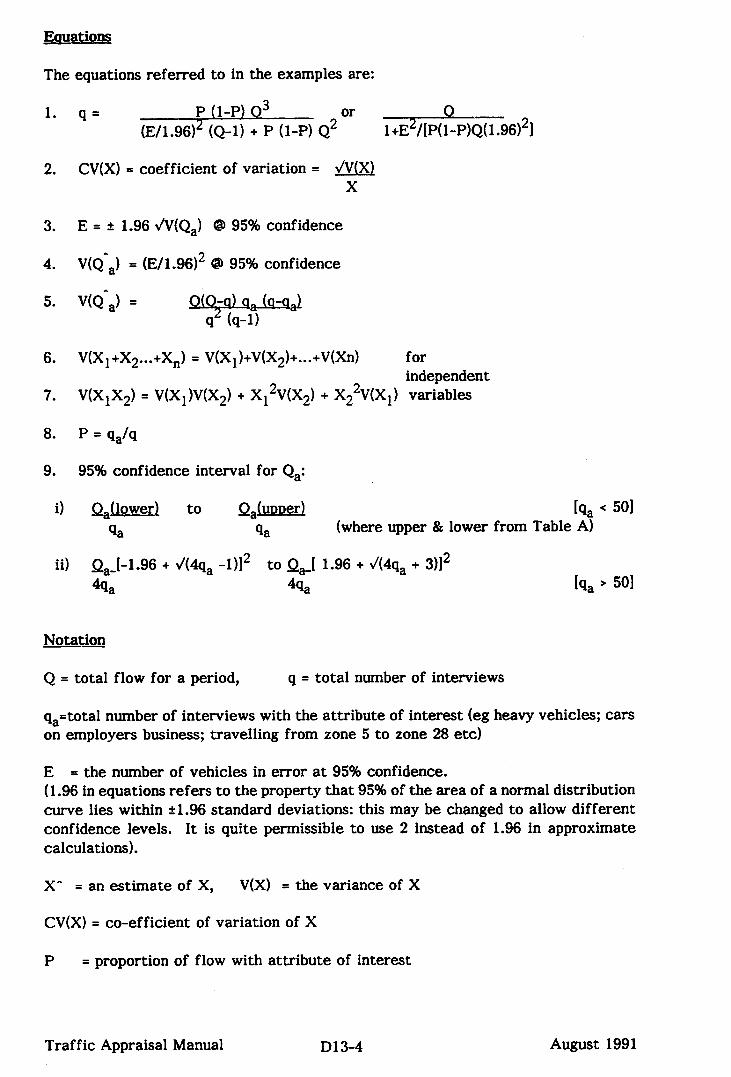
The equations referred to in the examples are:

1. q= P (1-P) o3 Or 0 (E/1.96)2 (Q-1) + P (1-P) Q2 l+E2/[P(l-P)Q(1.96)21

2. CV(X) = coefficient of variation = JV(X) X

3. E= + 1.96 &(Q,) 0 95% confidence

4. V(Q-a) = (E/1.96)2 @ 95% confidence

5. V(Q-,I =

6. V(XI+X2...+XJ = V(Xl)+V(X$+...+V(Xn) for independent

7. V(XlX,) = V(Xl)V(X2) + X12V(X2) + Xs2V(Xl) variables

9. 95% confidence interval for Qs:

i) QJlower) to Q.&nner) [qa ( 501

qa Qa (where upper & lower from Table A)

ii) Qa-[-1.96 + d(4qa -1)12 to Q,t 1.96 + J(4q, + 3)12

4qa 4qa [qa ’ 5ol

Notation

Q = total flow for a period, q = total number of interviews

q,=total number of interviews with the attribute of interest (eg heavy vehicles; cars on employers business; travelling from zone 5 to zone 28 etc)

E = the number of vehicles in error at 95% confidence. (1.96 in equations refers to the property that 95% of the area of a normal distribution curve lies within 21.96 standard deviations: this may be changed to allow different confidence levels. It is quite permissible to use 2 instead of 1.96 in approximate calculations).

X- = an estimate of X, V(X) = the variance of X

CV(X) = co-efficient of variation of X

P = proportion of flow with attribute of interest


Lo

\

TABLE A

‘b

Qa Lower UP1

0.0000 .0253 .242 .619 i nn 1.UJ

Q

3.69

5.57 7.22 8.77

tn r)~ &U.&-a

5 1.62 11.67 6 2.20 13.06 7 2.81 14.42 8 3.45 15.76 9 4.12 17.08

10 11 12 13 14

4.80 18.39 5.49 19.68 6.20 20.96 6.93 22.23 76x 39 AQ .."" LIV.1"

15 8.40 24.74 16 9.15 25.98 17 9.90 27.22 18 10.67 28.45 19 11.44 29.67

20 12.22 30.89 21 13.00 32.10 22 13.70 33.31 23 14.58 34.51 24 15.36 35,?1

25 16.18 36.90 26 16.93 38.10 27 17.79 39.28 28 18.61 40.47 29 19.42 41.65

30 20.24 42.83 35 24.38 48.68 40 28.00 54.47 45 32.82 60.21 50 37.11 65.92


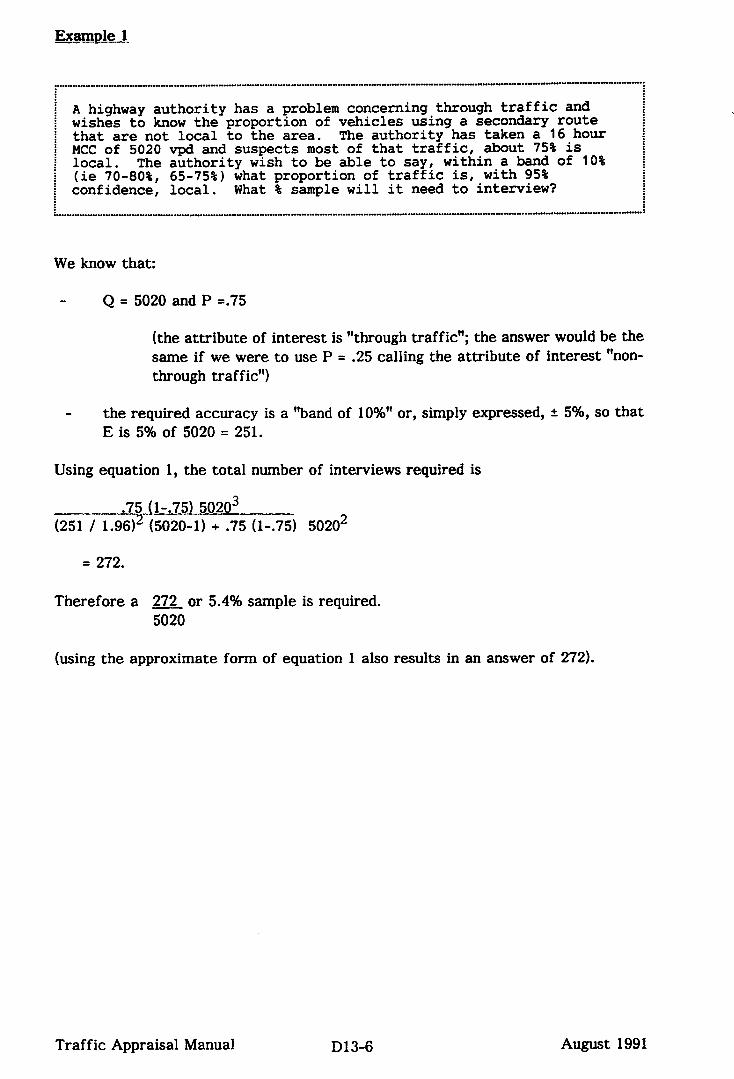
Exam-

. . . . . . . . . . . . . . . . . . ” . . . . . . . . . . . . . . . . . . . . . . . . . ” . . . . . . . . . . . . . . ” . . . . . . . . . . . . . . . . . . . . . . . . . . . . . . . . . . . . . . . . . . . . . . . . . . . . . . . . . . . . . . . . . . . . . . . . . . . . . . . . . . . . ” . . . . . . . . “ . . . . . . . “ ” . . . . . . . . . . . . . . . . . . . . s . . . . . . . . . . . . . “ . . “ . “ . . . ~

A highway authority has a problem concerning through traffic and wishes to know the proportion of vehicles using a secondary route that are not local to the area. The authority has taken a 16 hour MCC of 5020 vpd and suspects most of that traffic, about 75% is local. The authority wish to be able to say, within a band of 10% (ie 70-80%, 65-75%) what proportion of traffic is, with 95% confidence, local. What % sample will it need to interview?

. . . . . . . . . . . . . . . . . . . . . . . . . . . . . . . . . . . . . ..." . . . . . . . ..-................................................................... " . . . . . . . . . . . . . . . . . . . . .,.. . . . . . . - . . . . . ..." . . . . . . . . . . . I.."......"... . . . . . . . . . . .

We know that:

Q = 5020 and P =.75

(the attribute of interest is “through traffic”; the answer would be the same if we were to use P = .25 calling the attribute of interest “non- through traf f it?‘)

the required accuracy is a “band of 10%” or, simply expressed, + 5%, so that E is 5% of 5020 = 251.

Using equation 1, the total number of interviews required is

5020*

= 272.

Therefore a 272 or 5.4% sample is required. 5020

(using the approximate form of equation 1 also results in an answer of 272).


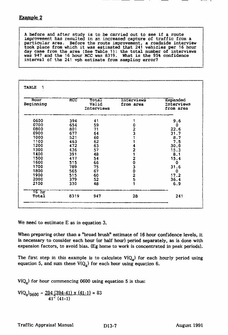
Examnle 2

: . . . . . . . . . . U.““.“...” . . . . . . . . . . . . . . . . . . . . . . . . . . . . . . . . . . . . . . . . . . . . . . . . . . . . . ..-.......................-... ” . . ...” _._. ““..._“.” . . .._ ““..“..“.-.“.......“....I....-... . . . . I . . . . . _...I.....

i A before and after study is to be carried out to see if a route i improvement has resulted in an i

inrtnscaa rsntllra of traffic from a . . . ..~_"_"I" vurr-r particular area. Before the route improvement, a roadside interview

i took place from which it was estimated that 241 vehicles per 16 hour i day came from the area (See Table 1): the total number of interviews i was 947 and the 16 hour MCC was 8319. What is the 95% confidence i interval of the 241 vph estimate from sampling error?

_....._........ ~.. ___.._I -I.-..ei......* . . . . . . . . . . . . . . . . . . . . . . . . . . . . . . . . . . . . . . . . . . . . . . . ...” . . . . . . . . . . ...” . . . . . I...” . . . . . . . . . . . “.,......“......“.._...“............s..”.”-”.....“...- . . . . . . . . . . . . . . . . . . . .

TABLE 1

Hour Beginning

MCC Total Interviews Expanded Valid from area Interviews

Interviews from area

0600 394 1 9.6 0700 654 :; 0800 801

:: 20 22'6

0900 677 3 31:7 1000 521 1 8.7 1100 463 :: 1200 472 63 : 3::; 1300 436 5? 2 15.3 1400 391 1500 417 ;: 1

8.1 15.4

1600 515 66 1700 789 z 31'6 1800 565 ::: i, 1900 515 60 ZD 17.2 2000 379 5 36.4 2100 330 :: 1 6.9

16 hr Total 8319 947 28 241

We need to estimate E as in equation 3.

When preparing other than a “broad brush” estimate of 16 hour confidence levels, it is necessary to consider each hour (or half hour) period separately, as is done with expansion factors, to avoid bias. (Eg home to work is concentrated in peak periods).

The first step in this example is to calculate V(Q,) for each hourly period using equation 5, and sum these V(Q,) for each hour using equation 6.

V(Q,) for hour commencing 0600 using equation 5 is thus:


and for all hours is:

From equation 6, the combined variance is:

‘(%)16 hour = 83 + 0 + 229 + 294.. + 128 + 211 + 40 = 1,838

and from equation 3 we have

E = r 1.96 d/1,838 = r 84.

The 95% confidence interval of the 241 estimate is then 241 + 84 (or 241 r 35%).


;

1 A 16 hour manual classified count has been undertaken to estimate i the 24 hour flow of cars on the day of the count. The 16 hour MCC

i

f gave 20000 vehicles. What is the 95% confidence interval of the 24 .i

i hour estimate? i

From section 6.3, the 95% confidence interval is given as + 10% for cars. The variance of the estimate of flow V(Q,) of 20000 vehicles is given by equation 4.

Where E = (10) x 20000 = 2000 (ie 10% of 20000) 100

V(Q,) = (2000 / l.96j2 = (lO20)2

Suppose the coefficient of variation for expansion of a 16 hour to a 24 hour count is 2.8% and the factor is 1.08. The estimate of 24 hour flow is thus: 20000 x 1.08 = 21600.

The variance of a product of variables is given in equation 7.

In the case X1 = 20000, X2 = 1.08,

V(X,) = 10202, V(X,) = (2.8% of l.0812 = (.0312

v(X,X,) = 10202(.03)2 + (20000)2 (.03j2 + l.082 (l020)2

V(X,X,) = 1574459

Using equation 3 we now have E, the estimate of error range at 95% confidence.

E = + 1.96 Jl574459 = f 2460

Therefore the 24 hour flow estimate of cars on a given day from a 16 hour MCC is 21600 f 11.4%.

(NOTE: The process can be further repeated to estimate AADT or AAWT etc).

Traffic Appraisal Manual Dl3-9 August 1991

“ “ ‘ “ “ “ “ ” . . . . “ . I . . . . . I . . . . . . . . . . . . . . . . I . . . . . “ . . . “ . “ “ ” . . . . . . . . . . . . . . . . . . I . . . . . . . “ ” . . . “ . . . ” . . . . . . . . . . ” . . . . . . . . . . . . . . . ” “ . . . “ . “ “ “ “ “ . “ “ “ . ~ . “ “ “ . “ ~ “ - . - - - “ “ . ” ” ” ” ” ” - ” - :

i During a study of movements in an off-peak base year traffic model i i where the matrix has been formed directly from roadside interviews, i f a traffic engineer wishes to understand the 95% confidence interval i of certain typical movements (as follows) from sampling error:

i

/ Station Zone(s) Zone(s) Unexpanded Expansion Estimated No I J Interviews Factor Tij . -----------------__-------------------------------------- 10 1 4 2 3.0 6

20 2 All zones 55 4.86 170

30 3 7+8+9 5 4.0 20 1 ) =32

40 3 7+8+9 2 6.0 12 1

40 All zones All zones 1057 6.06342 north south

: -------_____________-------------------------------------

Case 1

Taking the first case (zone 1 to zone 4 interviewed at Station lo), we establish that

qa = 2: the attribute of interest is travel from zone 2 to zone 4 and there are 2 interviews of this movement.

Now since qa < 50, we take equation 9i) to determine the 95% confidence interval for Q, (ie the estimated movement from zone 1 to zone 4 which is 6).

Referring to Table A, the lower limit value for qa = 2 is .242 and the upper value limit is 7.22 which when substituted into equation 9i) gives a 95% confidence interval between

5 x .242 and 5 x 7.22 2 2

= .726 and 21.66

thus the 95% confidence interval of the estimate 6 lies between 1 and 22.


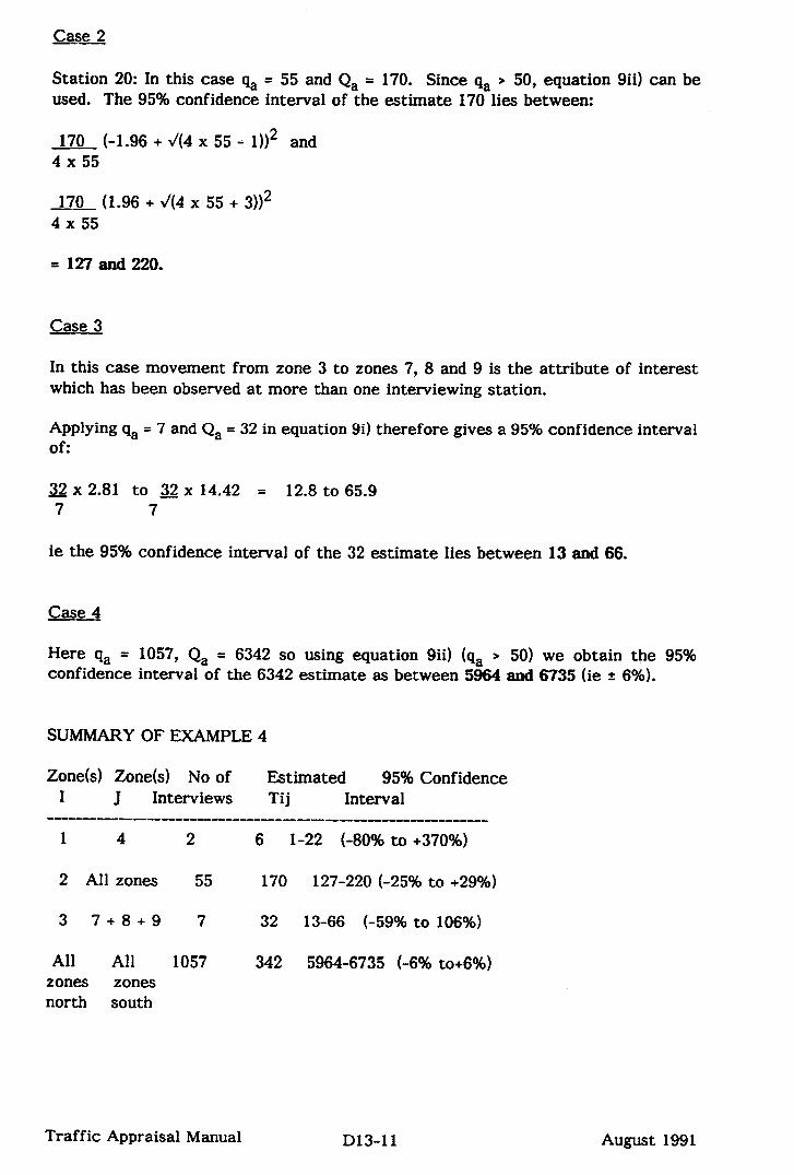
Case 2

Station 20: In this case qa = 55 and Qa = 170. Since qa * 50, equation 9ii) can be used. The 95% confidence interval of the estimate 170 lies between:

(-1.96 + d/(4 x 55 - l))* and 170 4 x 55

170 _ (1.96 + J(4 x 55 + 3))* 4 x 55

= 127 and 220.

Case 3

In this case movement from zone 3 to zones 7, 8 and 9 is the attribute of interest which has been observed at more than one interviewing station.

c-

‘--

Applying qa = 7 and Q, = 32 in equation 9i) therefore gives a 95% confidence interval of:

32 x 2.81 to 32 x 14.42 = 12.8 to 65.9 7 7

ie the 95% confidence interval of the 32 estimate lies between 13 and 66.

Case 4

Here qa = 1057, Q, = 6342 so using equation 9ii) (qa > 50) we obtain the 95% confidence interval of the 6342 estimate as between 5964 and 6735 (ie + 6%).

SUMMARY OF EXAMPLE 4

Zone(s) Znn&) _&l of Ectimsrtd QGqC. CnnfidDnPa -I.II*“bYY Y” I” -“‘*a l V”a*“e I J Interviews Tij Interval

____________________~~~~~~~~~~~~~~~~~~~~~~~~~~~~~~~~~~~~~~~~~

1 4 2 6 l-22 (-80% to +370%)

2 All zones 55 170 127-220 (-25% to +29%)

3 7+8+9 7 32 13-66 (-59% to 106%)

1 . . - -- _ ^_-

342 . ----

All All 1057 5964-6735 (-6% to+6%) zones zones north south


. . . . . . . . . . . . . ” . . . . ..s...........” . ...” . . . . . . . . . . . . . . . . . . . . . . . . . . . I.“...“..“..” . . . . . . . . . . . “.” . . . . . . . “.... . . . . . . . . . . I..... . . . . “........“.......“.“““.... .“..“...“.............a . . . ..I . . . . ““.“S

f A Highway Authority has built a new by-pass which it is just about ; to open. Using traffic orders the Authority confidently expects to I bar all by-passable traffic from the town. A roadside interview has : also just been undertaken at a neutral time of year (April) from i which 154 interviews out of a total of 384 have been classified as : "by-passable traffic"; 1

the total 16 hour flow through the interview station by manual count was 25100. What is the 95% confidence of

f AADT on the by-pass in the first year of opening? z......"."..." . . . . . . . . .."".."........" . . . . . . . . . . . . . . . . . . . . . . . . . . . . . . . . . . . . . . . . . . ..." . . . . . . . . . . . . . . . . . . . . . . ..." . . . . . . . . . . . . . . . . . . . ..."..." . . . . . . . . . . . . . . . . . "..... . . . . . . . . ..." . . . . . . ...** . . . . . "... . . . . G

In this example there are 3 types of measurement error:

i) measurement error in the manual count;

ii) sample error in estimating the proportion of by-passable traffic;

iii) sampling error in estimating AADT from a 16 hour count.

i) Measurement error From section 6.3, the measurement error in i) is + 10% @ 95% confidence, ie from equation 4,

V(Q,) = (.l x 25100 / 1.96)2 = (1280)2

where total flow is the attribute of interest being estimated.

ii) Samnle error From undertaking detailed calculations hour by hour as in Example 2 (data and calculations not shown) we could estimate that the sampling error in this case of the estimates of by-passable traffic, 10066 (ie 25100 x 154/384) is f 12.2% @ 95% confidence. The variance of the proportion of by-passable traffic (154 / 384 = .4) is thus

(.4 x (12.2 / 100) / 1.96)2 = (.025)2.

iii) Factor error From Appendix 2 of TRRL SR 514 (ref 3) we may take an M-factor (16 hour to total annual traffic) of 373 for a rural long distance traffic site which has an associated coefficient of variation of f 9.8%. The 16 hour to AADT factor is thus

373 / 365 = 1.02

and the variance =

LO98 x 1.0212 = .012.


The product of ii and iii has a variance, using equation 7, of

V(25100 x _lJ& x 10066) = (12802 x .02S2) + (251002 x .02S2) 384 + .42 x 1280 2 = 656924

where X1 = 25100; X2 = .4; V(Xl) = 12802; V(X,) = .02S2

The product of i) and ii) and iii) has a variance of

V(lOO662 x 1.02 = 10267) = (656924 x

(1 022 x 656;:) ;9,66”,““” x .O1) + . =

where X1 = 10066; X2 = 1.02; V(X,) = 656924; V(X,) = .012

Thus using equation 3, AADT = 10267 r 1632 (+ 16%) @ 95% confidence.


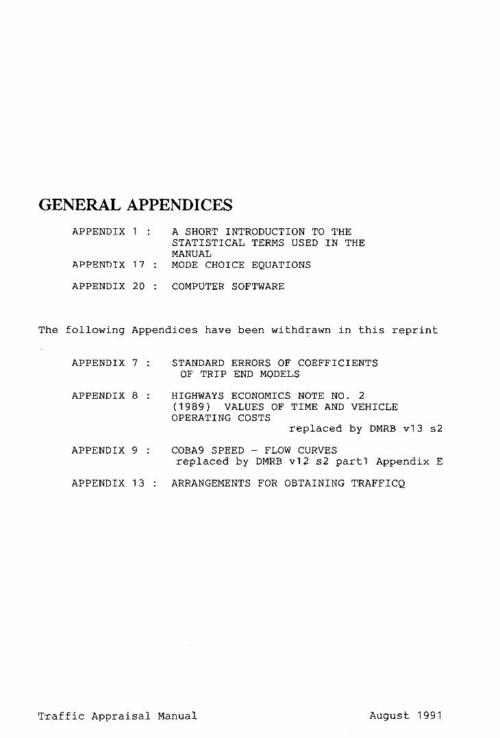
APPENDIX 1 : A SHORT INTRODUCTION TO THE STATISTTCAT TERMS USED IN THE L -__- --c _ - ___1

MANUAL APPENDIX 17 : MODE CHOICE EQUATIONS

APPENDIX 20 : COMPUTER SOFTWARE

The following Appendices have been withdrawn in this reprint

APPENDIX 7 :

APPENDIX 8 :

APPENDIX 9 :

APPENDIX 13 :

STANDARD ERRORS OF COEFFICIENTS OF TRIP END MODELS

HIGHWAYS ECONOMICS NOTE NO. 2 (1989) VALUES OF TIME AND VEHICLE OPERATING COSTS

replaced by DMRB v13 s2

COBA SPEED - FLOW CURVES replaced by DMRB v12 s2 part1 Appendix E

ARRANGEMENTS FOR OBTAINING TRAFFICQ

Traffic Appraisal Manual August i99i

APPENDIX 1: A SHORT INTRODUCTION TO THE SI’ATISTICAL TERMS USEDINTHEMANUAJa

Al.1 For a single variable the fundamental measure of error is the variance (o*): the expected squared error about the mean (equation 1 below). This is fundamental in the sense that the variance of the sum of two statistically independent variables is the sum of the two variances. The standard deviation (a) is the square root of the variance (equation 2), and has the same dimension as the variable itself. The standard deviation of the mean is often referred to as the standard error of the mean or s.e.(x) (equation 3).

Al.2 It is hard to think of any variable entering into traffic appraisal which can validly have negative values. For inherently positive variables, it is convenient to consider several measures relative to the mean. The ‘relative variance’ is the variance to square of mean ratio (equation 4). The dimensionless relative standard deviation is the standard deviation to mean ratio, usually referred to as the ‘coefficient of variation’ (equation 5). Whenever error is referred to as a percentage of the mean, it is probably the coefficient of variation which is meant.

Al.3 A further ratio, the variance to mean ratio (equation 6), or ‘index of dispersion’, has dimensions (those of the mean) and is often useful in summarising the error law of a variable as the mean changes (for example, it might be assumed that the variance bears a constant relationship to the mean, giving a constant index of dispersion). In particular if a l/S sample of a large population is taken at random, and n of the sample are found to have a particular attribute, the estimate Sn of the number in the whole population with the attribute has index of dispersion S. To understand an index of dispersion it has to be converted back into a standard deviation or coefficient of variation (equation 7).

Al.4 A basic understanding of statistics is useful for those involved with traffic appraisals. There are many standard statistical texts but particularly popular references are:

Moser C A and Kalton G: “Survey Methods in Social Investigation”, H E B Books;

Moroney M J: “Facts from Figures”, Pelican Books;

Hayslett H T: “Statistics Made Simple”, W H Allen; and

Hoe1 P G: “Introduction to Mathematical Statistics”, Wiley.

Confidence intervals are discussed further in section 6.1 of this manual.

Traffic Appraisal Manual Al-l August 1991

The estimate of the variance o2 from a sample of n measurements is given by:

S2 = &, t (XiwTlJ2 1=1

where Xi is the value of the ith measurement (i = 1,2,3,...n)

n is the number of measurements

ie x is the arithmetic mean of the n measurements

jT,1 n

c n l=l

xi

2. The estimate of the standard deviation u is given by

3. The standard error of the mean is given by

a2 s.e. (Z)= n J----

and estimated by J(S2/n) , where S2 is defined as in eq 1.

4. The relative variance is estimated by s2 / ‘;;2

5. The relative standard deviation is estimated by s / 2 This is usually expressed in percentage terms and referred to as the coefficient of variation:

ie c”=(s/x).100%

6. The variance to mean ratio, or index of dispersion is estimated by:

7.


s = JI’fsx

Al-2 August 1991

AF’FXNDIX 17 : MODE CHOICE EQUATIONS

A simnle techniaue to assess modal choice 0~~0rhmities

A17.1 The procedure for mode-choice described here is based on the gravity model formulation. The model should be applied to only that part of the population for whom a choice is available. In the absence of better information from a comprehensive study, it may be assumed that only people from car-owning households have a choice between public and private transport. The major input is person trips between zones and the output public transport person trips and private mode person trips. The latter is converted to vehicle trips by the application of car occupancy factors. The model is of the form:-

GiAj exp (-9Iijm) (1) T.. =

1Jm c jm

Aj em(-eI;j,)

where Tijm = trips from zone i to zone j by mode m;

Gi = generations from zone i;

Aj = attraction factor to zone j;

0 = a calibration constant that varies with trip Purpose;

I ijm = a measure of impedance between zones i and j by mode m; generally expressed as ( 1.0 x in-vehicle time ) + (w x out-of-vehicle time) + (trip cost) / (value of time)

W = conversion factor ( = 2 unless local data suggest otherwise);

and exp(x) = ex ; e = 2.71828

A17.2 From this equation it is possible to directly determine the proportion of trips made by public transport:-

mst

expkJ =

expt-BIt) + exp(BI 1 - c

= 1 (2) 1+ exp(8 (It - I,))

Traffic Appraisal Manual A17-1 August 1991

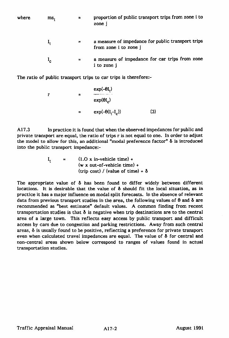
where = proportion of public transport trips from zone i to zone j

It = a measure of impedance for public transport trips

from zone i to zone j

= a measure of impedance for car trips from zone i to zone j

The ratio of public transport trips to car trips is therefore:-

r exd-BIJ

= expO31,)

= exp(-B(It-I,)) (3)

A17.3 In practice it is found that when the observed impedances for public and private transport are equal, the ratio of trips r is not equal to one. In order to adjust the model to allow for this, an additional “modal preference factor” 6 is introduced into the public transport impedance:-

I, = (1 .O x in-vehicle time) + (w x out-of-vehicle time) + (trip cost) / (value of time) + 6

The appropriate value of 6 has been found to differ widely between different locations. It is desirable that the value of 6 should fit the local situation, as in practice it has a major influence on modal split forecasts. In the absence of relevant data from previous transport studies in the area, the following values of 8 and b are recommended as “best estimate” default values. A common finding from recent transportation studies is that b is negative when trip destinations are to the central area of a large town. This reflects easy access by public transport and difficult access by cars due to congestion and parking restrictions. Away from such central areas, 6 is usually found to be positive, reflecting a preference for private transport even when calculated travel impedances are equal. The value of 6 for central and non-central areas shown below correspond to ranges of values found in actual transportation studies.


Trin Purnoses

home-based work (HBW)

home-based other (HBO)

non home-based (NHB)

CA = Central Area

A17.4 This simple model is suitable for application to most trunk road schemes serving local functions. However, for the minority of schemes where a significant proportion of trips is longer than about 25 miles, the ability of the model to perform satisfactorily cannot be assumed. In such cases EEA Division in HQ should be consulted.

Selection of Study Area and Zoniw System

A17.5 Define the area likely to be affected by the scheme. Using the national or local zoning system select those zones which cover the area of interest. Zones should be aggregated to give the minimum number possible, subject to the following constraints:-

i) Zones should be limited in size so that the longest access distance from any significant concentration of population to public transport service (eg bus stop or railway station) is not more than 2.5 km, and the diameter of the populated area should not exceed 5 km.

ii) It is desirable in most cases to have separate zones feeding into distinctly different public transport services (eg different railway stations, or bus routes on widely separated - more than 2 km - roads).

iii) The zoning system should be compatible with the zoning system of any other data sources to be used in the study.

Select zone pairs between which it is desired to investigate trips. Trips between some zone pairs in the zoned area will not be affected by the scheme, and are therefore not relevant to the scheme appraisal. Such zone pairs should be noted, and no data need be collected from them.

Traf fit Appraisal Manual A17-3 August 1991

Data Reauh-ed for AIx&ation

A17.6 Theusezmustmakeeveryefforttotakeadvantageoflocal modelsand parameter values. Only where such information is not available should default values be used. Table 1 lists the data items required for the application of the mode choice procedures. In the majority of cases most of these data items will already be available eg highway distances, costs from skim trees. There may also be instances when zone to zone travel impedances are available. In such cases the particular calculation steps described in the following sections will be unnecessary.

A17.7 Notes on items in Table 1:

Highway Distance The straight-line distance between zone centroids can be directly scaled off from maps. Road distances can be estimated as 1.22 x straight-line distance. Alternatively, actual distances can be measured on a map.

INPUT DATA ITEMS

Highway distance

Public transport connection

Public operating cost

Vehicle operating cost

Attraction end parking cost

Matrix of zone to zone private transport trip times

Matrix of zone to zone public transport trip

Values of coefficients 8 and 6

Median income

Access time

TABLE 1.

Public TransDort Connection Zone pairs without public transport service should be identified and eliminated from the analysis.


Public Transnort Fares A matrix of zone to zone public transport fares should be built up from knowledge and supplemented by information from service operators’ published fare tables.

Vehicle OneratinP Costs The latest values developed by EEA should be used to compile the vehicle cost matrix.

Attraction End Parkinn Cost Trip duration varies by purpose and consequently parking costs will be necessary for each trip purpose. As a guide, a nine hour duration may be assumed for HBW and two hours for HBO and NHB. These values have been adopted from recent transportation studies. Half the actual parking charges associated with a round trip should be used in the calculations. The parking costs for a zone should be developed on the b

r is of

all available parking (free and paid) in a zone for each trip purpose or altem ,tively the definition of a separate purpose for those with free and those with paid parking in city centres should be made. This is a matter for local judgement.

Matrix of Zone to Zone Private Transnort TriD Times This may be available from previous studies in the area, with suitable estimates for updating if necessary. If no such data are available, times will have to be calculated from a knowledge of highway distances and observed or estimated average speeds.

Matrix of Zone to Zone Public Transnort Trin Times To matrix of zone to zone public transport trip times can be built up from local knowledge and the use of public transport operators’ time-tables. There may be instances where local conditions such as severe congestion or other operating difficulties cause major differences between published time-tables and the service actually provided. In such cases suitable adjustments should be made to the estimate of trip times. This is a matter for local judgement. Some zone pairs will be found to have no convenient public transport service even by making interchanges. In such cases the estimated number of public transport trips would be zero. It is assumed that all trips from such zone pairs would be made by private mode either as drivers or passengers. These movements can therefore be eliminated from the analysis. If the service differs significantly between the peak and off-peak periods, separate service descriptions would be required. As a general rule, the peak system would apply to the HBW trip purpose whilst the off-peak system would apply to the HBO and NHB trip purposes.

Values of Coefficients 6 and 6 In the absence of local information the default values given earlier in section 1 should be used.

Median Income The median income value is required to determine the value of time for conversion of vehicle operating costs, parking costs and public transport fares to equivalent minutes. National values should be used only if local estimates are unreliable or unavailable. For studies where this simple technique is applicable a single value of median income may be used for the whole study area.


Access Time Access time is the time between leaving the origin to entering the vehicle (public transport or private) plus the time between leaving the vehicle and reaching the trip destination. For public transport trips, it will include waiting time and it may also include time to transfer between vehicles. This is also referred to as out-of-vehicle time. Waiting time is normally estimated to be half the headway between services.

Person Trip Table A zone to zone person trip matrix is required for each trip purpose to be analysed. It may be assumed that trips in the peak period are for HBW purpose and trips outside the peak period are for the combined OHB and NHB purposes. It is assumed that public transport usage by passengers without a choice of mode will not be affected by highway improvements or public transport service changes.

A17.8 Therefore, only public transport trips by persons for whom a choice of mode is available need be considered for the purposes of the assessment described here. In order to estimate the number of public transport passengers who have a choice of mode, two approaches are possible depending on the data that is available:-

i) A zone to zone matrix of trips by all persons from car-owning households. It is assumed that such persons have a choice of mode. This matrix might be derived by the use of household interview data or data from the Census of population in a simple trip distribution model. The number of public transport passengers (with choice of mode) could be obtained from this by estimating the value of mst (the proportion of all person trips made by public transport).

ii) A zone to zone person trip matrix of all people travelling by private transport. This would normally be available from roadside interview surveys, supplemented by traffic counts. If a private vehicle trip matrix is available then it should be converted to a person trip matrix by the use of appropriate vehicle occupancy factors. The number of public transport passengers could be derived from this by estimating the value of r (the ratio of public transport to private transport person trips).

Amkation of the procedurerr qmde-choice estimation

A17.9 Figure 1 is a generalised flow chart of the procedure to be adopted. The procedure cycle shown in Figure 1 must be completed once for each trip purpose. The three main steps of the procedure are:-

Determine nrivate and nublic traniort imDeda=

A17.10 The first and most difficult task is the determination of the zone to zone impedances. Figure 2 shows “Work Sheet A” used for the application of the procedures.


In some cases it may be possible to reduce the level of effort by compressing the square person-trip table into a triangular one and summing the trips to the total movement between i and j; if travel characteristics between i and j are assumed to be equal to j to i. This may not be true in many areas where the inbound public transport service may differ markedly from the outbound service as in peak period commuting, destination parking costs are likely to be different, etc. In such cases no attempt must be made to reduce the square person-trip table to a triangular one.

A17.11 The following information should be entered for each zone pair; public transport fare (F), highway distance (D,), public transport trip time (Tt), car (private transport) trip time (T,), public transport access time (A,), car access time (A,), public transport fare divided by value of time (F/V), parking cost (P,) divided by the value of time (P/V), and the highway distance times vehicle operating cost (V,)

divided by the value of time (Dc x V,/V).

Calculate the public transport and car impedance values:

I, (public transport impedance) = T, + (w x At) + F/V)

I, (car impedance) = T, + (w x Ac) + P,/V + (Dc x V,/V)

where V = value of time

w = conversion factor (=2 unless local data suggest otherwise)

Enter these values on the work sheet.

Determine Public Transst Mode Share

A17.12 Depending on the nature of the person trip data to be used (see 3.111, it is necessary now to estimate either the value of public transport mode share (ms,) or the ratio of public to private transport mode shares (r). If a programmable calculator is available mst and r can be calculated from equations (2) and (3) respectively (see section 1) using appropriate b values in the public transport impedances (It). Alternatively mst can be read off Fig 3 and r off Fig.4


Determine Public Transnort and Car Persons-Trins

A17.13 Depending on the data available:

i) If a matrix of total person trips by those with a choice of mode is available then Work Sheet B shown on figure 5 should be prepared. The total person trips between pairs of zones for the trip purpose under investigation should be recorded on the work sheet, also the percentage public transport share (mst). Multiplying the total number of trips by mst will give the number of public transport person trips expected to occur between zones. Subtracting the public transport person trips for that particular zone pair from the total person trips will yield the number of private (car) person trips for the zone pair.

ii) If a matrix of person trips by private transport is available then Work Sheet C shown on figure 6 should be prepared. The number of private transport person trips (N,) between pairs of zones for the trip purpose under investigation should be recorded on the work sheet. The value of the ratio of public to private transport mode shares (r) should also be entered on the work sheet. Multiplying N, by r gives the number of public transport person trips (Nt) for that particular zone pair.

The completion of Work Sheet B or Work Sheet C finishes the mode-choice analysis for the trip purpose. The procedure is repeated for each trip purposes.


PRIVATE IMPEDANCE DETERMINATION

l Vehicle time matrix

@Vehicle cost matrix

l Access time and parking cost

l Private impedance

PUBLIC TRANSPORT IMPEDANCE DETERMlNATlOh

l Public transport trip time matrix

l Fare matrix

l Access and waiting times

l Public Transport impedance

for appropriate trip

BASIC METHODOLOGY

Public Transport and Private Person-Trip


AND ZONE

T-

lie Transport tare

C = Car (Highway) distance

t Public Transport trip time

Tc -Car trip time

Lt = Public Transport acooas time

Zar access time

= Parking cost

Iii Transport impodanom (@min

impodanco (oquiv.miu.)

ick operating Coat

I&)

+ If triangular work sheet is required, all cells vertically below the shaded cells should be eliminated

It=Tt +(wxAt)+F/v

Ic=Tc+(wxAc)+Pc/y+(DcXVc/v)

w I 2 (unless local data suggest otherwise)

mst should be replaced by r( the ratio of public to private transport

mode shares) where appropriate

Work Sheet A

FIG. 2


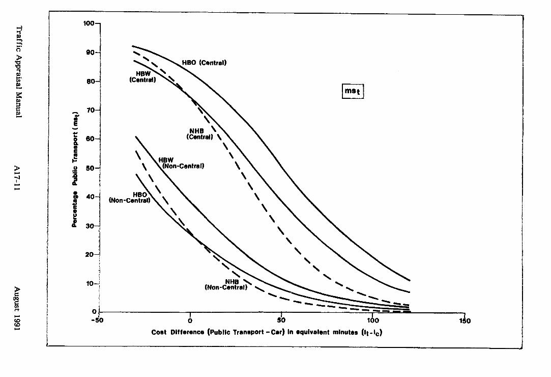
80

I I 0 60

Cost Difference (Public Transport -Cer) In equivalent minutes (It-l,) Cost Difference (Public Transport -Cer) In l qulvalent minutes (It-l,)

I I 8 0

I ” 7

\ g

\ \’ \ \ 2

\

\

\

\z, :

\P Is

\; ;

\* 5 \% =

-.

Cost dlfterence (Public Transport - Car) In equivalent mtnutes (It- 1,)


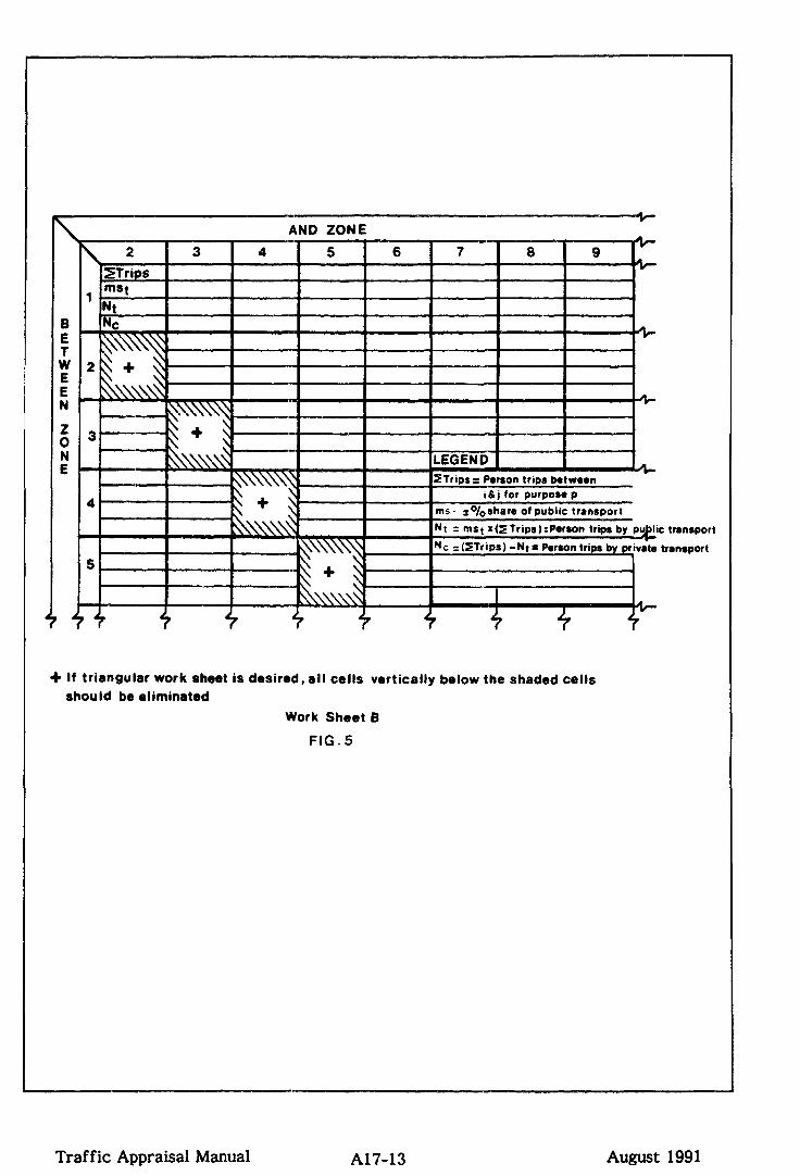
AND ZONE

Efripsz Person trips batwoen

IC tranrport

transport

+ If triangular work sheet is desired, all cells vertically below the shaded cells

should be eliminated

Work Sheet 8

FIG.5


AND ZONE

person lr10s

+ If triangular work sheet IS desrred. all cells vertically below the shaded cells should be ellmmated

Work Sheet C

FIG.6

Traffic Appraisal Manual Al?-14 August 1991

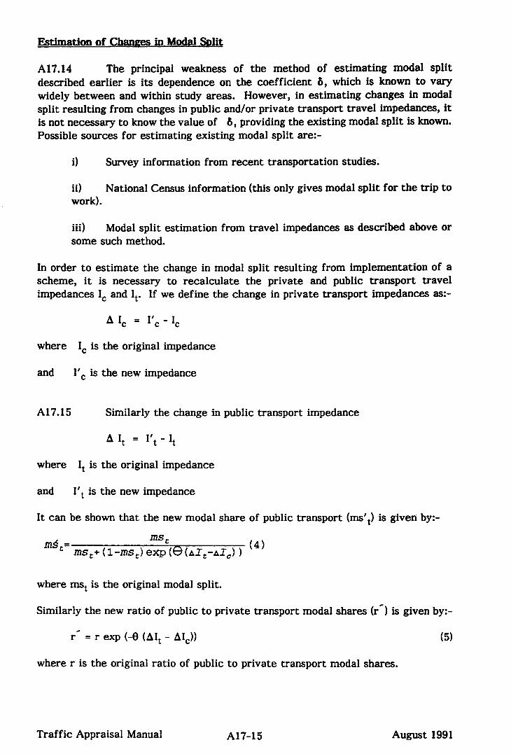
Estimation of Chmes in Modal Slit

r- = r exp (-9 (AI, - AI,))

Al7.14 The principal weakness of the method of estimating modal split described earlier is its dependence on the coefficient 6, which is known to vary widely between and within study areas. However, in estimating changes in modal split resulting from changes in public and/or private transport travel impedances, it is not necessary to know the value of b, providing the existing modal split is known. Possible sources for estimating existing modal split are:-

i) Survey information from recent transportation studies.

ii) National Census information (this only gives modal split for the trip to work).

iii) Modal split estimation from travel impedances as described above or some such method.

In order to estimate the change in modal split resulting from implementation of a scheme, it is necessary to recalculate the private and public transport travel impedances I, and I,. If we define the change in private transport impedances as:-

A I, = I’, - I,

where I, is the original impedance

and I’, is the new impedance

Al7.15 Similarly the change in public transport impedance

A I, = I’, - I,

where I, is the original impedance

and I’, is the new impedance

It can be shown that the new modal share of public transport (ms’,) is given by:-

mst m~C~mst+~l-mst~exp(~(~It-~lZ,)) (4)

where mst is the original modal split.

Similarly the new ratio of public to private transport modal shares (r-1 is given by:-

where r is the original ratio of public to private transport modal shares.

Traffic Appraisal Manual Al7-15 August 1991

A17.16 These values can either be calculated, if a programmable calculator is available, or values of ms-t read off figures 7 and 8 for home based trips (work and other) and NHB trips respectively and r* can be read off figures 9 and 10 for home based trips (work and other) and NHB trips respectively. Work sheets similar to those in figures 5 and 6 may be prepared if they are considered to be useful in aiding the computational effort.


100

90,

90

70

90

so

w

30

20

lo

Q

CHANGES IN PUBLIC TRANSPORT SHARE

DUE TO CHANGES IN COST DIFFERENCE [A(&/&]

IN EQUIVALENT MINUTES


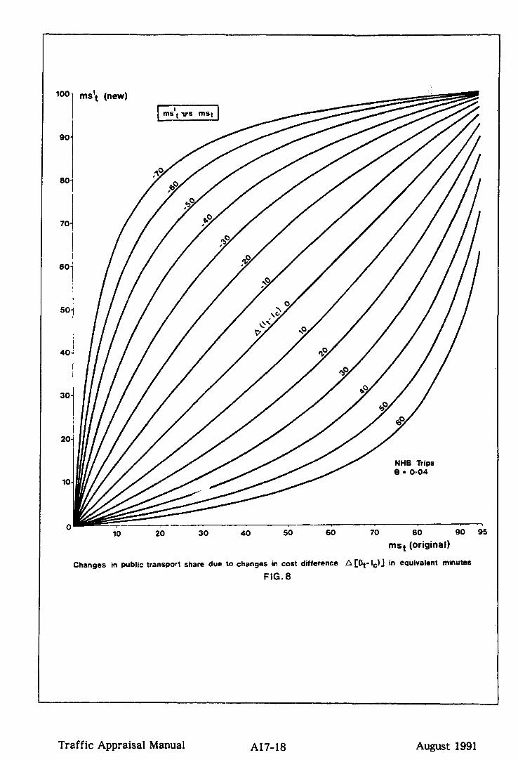
100 1 rnsi (new)

10 20 30 40 50 60 70 00 90 95

mst (original)

Changes in public transport share due to changes in cost difference A [(It- Ic)J in equivalent minutes

FIG.8


2+ r’ (new)

2.5

2.4-

2.3-

1-8-

Home based trips (work and other)

"0 .i .j .h .j .b .i .g 1:o 1; 112 1:3 19 1.5 l-6 l-7 :

Changes in modal ratio due to changes in cost difference [AtIt-I,)] in equivalent minutes r&i$w;l)g


CheWor in model mtio due to chenges in cost difference A [(It-lc.] in l quivelent minutes I (originat)

FIG. 10


APPENDIX 17.2: PROBLEMS ENCOUNTERED IN THE DEVELOPMENT OF A SIMPLE MODAL SPLIT MODEL

A17.17 The purpose of a ‘simple’ modal split model is to enable estimates of modal split (or of changes in modal split) to be made in circumstances where only very limited survey data is available. It is assumed that such data would be insufficient to calibrate a model (ie estimate the values of the model coefficients) so that recourse has to be made to past experience of modal split modelling.

A17.18 In the last ten years there have been many major transportation studies in the UK in each of which a great amount of survey data has been collected and modal split models have been calibrated. In principle therefore there should be more than sufficient information from which to develop a ‘simple’ model. In practice it is very difficult to reconcile information from different studies and to produce a common model applicable to all situations. The problems are of two kinds, structural and numerical.

Structural Droblems

A17.19 Almost every transportation study has some unique features in its model structure which make it different from any other transportation study. These differences have occurred for a number of reasons, including local peculiarities in the region being studied, an improving understanding of the modelling processes, personal preferences of the consultants involved, and availability of particular computer program suites. The main dimensions along which differences have occurred are market segmentation, the simultaneous/sequential structure, and the use of analytical or empirical deterrence functions.

Market segmentation

A17.20 Instead of developing a single model to cover all types of trip, it is usual to develop a set of models, each of which is matched to a particular type of trip. Normally all the models would have the same basic structure, but would have different values for the estimated coefficients. Such market segmentation usually differentiates between different trip purposes (eg work, home-based non work, non home-based, etc) and between different person types, the latter commonly being defined in terms of household car ownership (eg no car, one car, two or more cars). Unfortunately different studies have used widely varying degrees of complexity of market segmentation, and even where the number of divisions (eg in trip purposes) are the same, the actual classification boundaries differ slightly. It is therefore very difficult to obtain exact comparisons between the estimated coefficients for different studies.


Simultaneous/seauential model structures

A17.21 The traditional ‘four stage’ model used in many transportation studies uses separate sub-models, applied sequentially, for each of the stages; trip generation, trip distribution, modal split, and assignment (route choice). In such cases the modal split sub-model can be used as an independent model, which is directly applicable in any comparison between modal split models. However, in some studies a combined distribution / modal split model has been used, in which both operations are carried out simultaneously. In some cases there have been problems in deriving an equivalent independent modal split model which can be used for comparative purposes.

Analvtic and emuirical modal snlit functions

A17.22 in the early days of transport modelling, modal split was sometimes derived as a function of the ratio of generalised costs (impedance) for travel by alternative modes, and sometime as a function of the difference of generalised costs.

In more recent studies, the use of cost ratios as a determinant of modal split has been abandoned, and all modal split models depend on a function of generalised cost differences. There are good theoretical grounds for preferring this form, but it is not known whether there has ever been a conclusive demonstration from survey results that this form actually provides a better fit to reality than the cost ratio form. It is not in general possible to equate the two forms exactly, due to the impossibility of finding sets of coefficients which will cause the two types of model to predict both the same modal split and the same elasticity. However, over a limited range of costs an acceptable approximation may be possible.

A17.23 Ideally modal split would be presented as a smooth curve showing the relationship between the proportion of trips by a particular mode and the difference in generalised costs. In practice there is usually considerable scatter of individual points plotted to show the relationship. The majority of transportation studies assume that the relationship follows a logit curve, and ‘calibration’ consists of estimating the values of the coefficients which give the ‘best fit’ logistic curve. Some studies have not attempted to use an analytic approximation, and have drawn an empirical ‘best fit’ curve through the data points; this curve is then presented as a ‘diversion curve’ to be used for forecasting future modal splits in the region. These studies do not generally describe the statistical method by which the empirical curve is produced. In order to compare the results of studies of this type with studies in which logit coefficients are derived it is necessary to estimate a ‘best fit’ logit equation for the empirical curve. This is statistically unsatisfactory, compared with estimating the logit coefficients from the original data points.


4

4

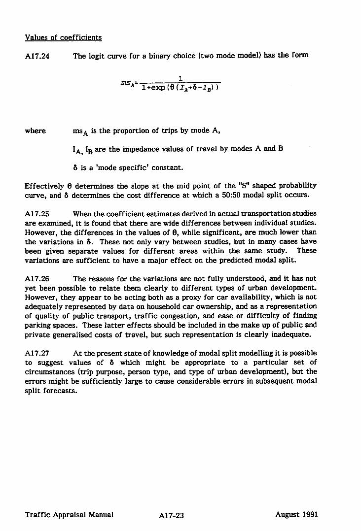
Values of coefficients

A17.24 The logit curve for a binary choice (two mode model) has the form

msA= 1 +exp (8 (iA+* -IB) )

where msA is the proportion of trips by mode A,

IA, IB are the impedance values of travel by modes A and B

8 is a ‘mode specific’ constant.

Effectively 6 determines the slope at the mid point of the “S” shaped probability curve, and 6 determines the cost difference at which a 50:50 modal split occurs.

A17.25 When the coefficient estimates derived in actual transportation studies are examined, it is found that there are wide differences between individual studies. However, the differences in the values of 6, while significant, are much lower than the variations in b. These not only vary between studies, but in many cases have been given separate values for different areas within the same study. These variations are sufficient to have a major effect on the predicted modal split.

A17.26 The reasons for the variations are not fully understood, and it has not yet been possible to relate them clearly to different types of urban development. However, they appear to be acting both as a proxy for car availability, which is not adequately represented by data on household car ownership, and as a representation of quality of public transport, traffic congestion, and ease or difficulty of finding parking spaces. These latter effects should be included in the make up of public and private generalised costs of travel, but such representation is clearly inadequate.

A17.27 At the present state of knowledge of modal split modelling it is possible to suggest values of 6 which might be appropriate to a particular set of circumstances (trip purpose, person type, and type of urban development), but the errors might be sufficiently large to cause considerable errors in subsequent modal split forecasts.


Conclusion

A17.28 It appears possible to develop a simple modal split model which would use only limited data on travel times and costs as an input. However, the errors of forecasting modal split by such a model could be considerable, and its value will depend on its intended use. The addition of any data on actual modal split in the relevant area could considerably improve the forecasting accuracy of such a model, as this would eliminate the large and unknown bias caused by errors in 6. Possibly census information could be used to provide such data for peak hour trips to work. It seems likely that the use of such data could also improve forecasting accuracy for trips made for other purposes, for which no survey data is likely to be available.

Traf fit Appraisal Manual A17-24 August 1991

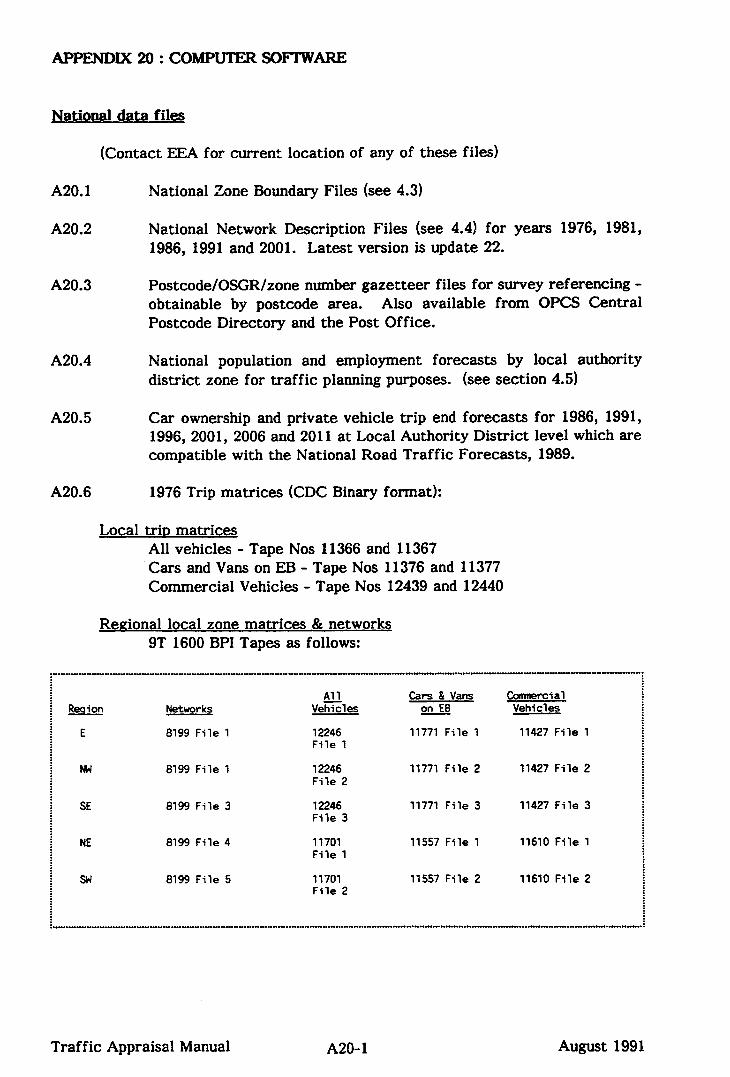
L

APPENDIX 20 : COMPUTER SOFIWARE

National data files

(Contact EEA for current location of any of these files)

AZO. 1

A20.2

National Zone Boundary Files (see 4.3)

National Network Description Files (see 4.4) for years 1976, 1981, 1986, 1991 and 2001. Latest version is update 22.

A20.3 Postcode/OSGR/zone number gazetteer files for survey referencing - obtainable by postcode area. Also available from OPCS Central Postcode Directory and the Post Office.

A20.4 National population and employment forecasts by local authority district zone for traffic planning purposes. (see section 4.5)

A20.5 Car ownership and private vehicle trip end forecasts for 1986, 1991, 1996, 2001, 2006 and 2011 at Local Authority District level which are compatible with the National Road Traffic Forecasts, 1989.

A20.6 1976 Trip matrices (CDC Binary format):

Local trin matrices All vehicles - Tape Nos 11366 and 11367 Cars and Vans on EB - Tape Nos 11376 and 11377 Commercial Vehicles - Tape Nos 12439 and 12440

Regional local zone matrices & networks 9T 1600 BP1 Tapes as follows:

L

Reqion

E

All Cars & Vans Cunnercial

Networks VeKles on E8 Vehicles

8199 File 1 12246 11771 File 1 11427 File 1 File 1

Nn 8199 File 1 12246 11771 File 2 11427 File 2 File 2

SE 8199 File 3 12246 11771 File 3 11427 File 3 File 3

NE 8199 File 4 11701 11557 File 1 11610 File 1 File 1

SW 8199 File 5 11701 11557 File 2 11610 File 2 File 2

Traffic Appraisal Manual AZO-1 August 1991

1976 Comnressed matrices County and District compressions of the 1976 trip matrices are available by purpose and vehicle type in both CDC Binary and Character .Format. Further details are contained in Traffic Appraisal Procedure Note 2.

List of Programs

A20.7 ROADWAY Suite of Portable Traffic Modellinn Software

RDNET RDTREE

RDSKIM

RDTAB RDSIFT

RDBILD

RDTRIP

RDGRIN

RDGRAV2 RDMAT RDFLOW

RDSELC

RDCOMP

RDPLOT RDEVAL

A program to define or update a road network. A program to print trees for selected zones and if required generate a file for plotting. A program to produce a zone to zone time, distance or generalised cost matrix. A program for the analysis and tabulation of survey data. A program to select trip information from an RHTM Data Bank file or other user supplied data file. A program to build a matrix from a file output by RDSIFT, RDTAB or RDTMAT. A trip end estimation program using category analysis techniques. A program to re-order the output from RDTRIP or ROUTE Suite program REGTRIP for input to RDGRAV. A trip distribution program using a gravity model formulation. A matrix manipulation program. A program to produce traffic flows on links or turning flows at selected intersections. A program to print a matrix of flows using a selected link or links crossing a specified cordon. A program to compare an identify the differences between two networks or loaded networks. A program to plot a network, loaded network or selected tree. An economic evaluation program using consumer surplus techniques.

A20.8 ROADWAY Sunnlementarv Prozrams

RDTNET A program to create a ROUTE Suite network transfer file for input to RDNET.

RDTMAT A program to create a ROUTE Suite matrix transfer file for input to RDBILD.


In addition, a complementary package of trip matrix building and validation programs

is under development and is due for release in 1981 comprising the following:-

RDRISP * A program to extract selected trip information from a roadside interview data file for input to RDMVAR.

RDHISP * As above for household interview data. RDMVAR A program to build trip matrices and calculate matrix cell

variances. RDMERG A program to merge two matrices using a ‘minimum coefficient

of variation’ criterion. A variance matrix for the merged matrix, is produced.

RDCOSM The comparison of two matrices, or examination of a single matrix, using a wide range of statistical measures.

* - these programs will replace RDSIFT in the original suite

A20.9 COBA economic evaluation interface nrograms

A complementary package of portable software to interface ROADWAY output with the COBAS ‘economic evaluation package is under development together with some diagnostic programs: these are due for release in 1981 and comprise the following:

BINT - Converts traffic model output into COBAS form. SWOP - Produces COBAS input data format file. NETBEN - Produces a consumer surplus economic evaluation for a network

compatible with COBA for a given year. MATBEN - Calculates zonal journey costs and benefits using COBA

parameters. COJUNC - Analyses junction delay costs. EDITURN - Analyses turning movement matrices.

A20.10 The following diagram shows the relationship between the ROADWAY programs:

NB: A broken line indicates that the file is optional input to or output from the indicated program.

For reasons of clarity, output trip matrix files in a block are shown repeated as input trip matrix files in another block, and flow lines between them omitted.

All programs have associated card input and line printer output files. These have been omitted here for reasons of clarity.

In all cases where a network file is shown as input to a program, a loaded network file may be input instead if required.


iiiRvEY ANALYSIS AND MA?RlX BUILD)%

rwalx

L-J

-------, mulLma

: , I :

TRIP OlSTRlBUllON ;

MATRIX MANIPULATION

I

I

;

m - - - m h , - - - - - -

I

I

I

I I 1 I I I I I I I

I _ I I c--...., i 1 ----- I

NETWORK DE6N;TION AN0 ANALYSIS

LSSIGNMENT AND FLOW ANALYSIS I

7 !I

1RlC

".,*,=

ECONOMIC EVALUATION


the aplicacion of traffic appraisal to trunk roads shemes

Documents