the analytics of technology news shocks - …smehkari/mainpaperdm.pdfthe analytics of technology...

The Analytics of Technology News Shocks∗

Bill Dupor† and M. Saif Mehkari‡

July 2014

Abstract

This paper constructs several models in which, unlike the standard neoclassical growthmodel, positive news about future technology generates an increase in current con-sumption, hours and investment. These models are said to exhibit procyclical newsshocks. We find that all models that exhibit procyclical news shocks in our paper havetwo commonalities. There are mechanisms to ensure that: (I) consumption does notcrowd out investment, or vice versa; (II) the benefit of forgoing leisure in responseto news shocks outweighs the cost. Among the models we consider, we believe, onemodel holds the greatest potential for explaining procyclical news shocks. Its criticalassumption is that news of the future technology also illuminates the nature of thistechnology. This illumination in turn permits economic actors to invest in capital thatis forward-compatible, i.e. adapted to the new technology. On the technical side, ourpaper reintroduces the Laplace transform as a tool for studying dynamic economiesanalytically. Using Laplace transforms we are able to study and prove results aboutthe full dynamics of the model in response to news shocks.

JEL classification: E3Keywords: Business Cycles, News Shocks, Laplace Transforms.

∗The authors would like to thank Paul Evans, Jang Ting Guo, Jing Han, Alok Johri, Aubhik Khan, Nan Li, Masao Ogaki,

Hammad Qureshi, Julia Thomas, Yi-Chan Tsai, and conference and seminar participants at the Federal Reserve Bank of St.

Louis, the University of Western Ontario and the Midwest Macroeconomics Meetings. The analysis and conclusions set forth

do not reflect the views of the Federal Reserve Bank of St. Louis, the Federal Reserve System or the Board of Governors.†Research Division, Federal Reserve Bank of St. Louis, P.O. Box 442, St Louis MO 63166-0442, USA. Email:

[email protected]; [email protected]‡Department of Economics, Robins School of Business, University of Richmond, Richmond VA 23173, USA. Email:

[email protected]

1

1 Introduction

The optimal response of aggregate consumption, investment and hours in the neoclassical

growth model to an unanticipated permanent (or near permanent) technology increase is

well-understood. For most specifications used by researchers, all three variables increase.1

A technology improvement increases capital’s efficiency; thus, the desired capital stock in-

creases. The increase in the actual capital stock towards its desired level is achieved by

greater investment. Importantly, greater investment need not come at the cost of a drop in

consumption. Rather, since the technology improvement shifts out the production frontier

immediately, creating additional consumption and investment is feasible. Moreover, an hours

increase is optimal because a higher marginal product of labor induces a substitution effect

away from leisure that outweighs the wealth effect, which pushes in the opposite direction.

Next, consider the standard growth model’s response to news of a future technology

increase. The responses of these variables and the incentives that drive these responses are

different. In the standard model, all three variables will not increase. Typically, labor falls

upon the arrival of the news. The above-described wealth effect on leisure is operative;

however, there is no offsetting substitution effect because the technology increase has not

materialized immediately.

With a labor decline, the only way consumption can increase in response to the news

is if investment falls. An investment decline is optimal because there is incentive to delay

building additional capital stock until technology actually increases. Thus, in the standard

model, positive news about future technology can cause a decline in labor and investment,

and an increase in consumption (see Figure 1).2,3

[Insert Figure 1 here]

1Campbell [11] establishes this by simulation using several functional forms of preferences and modelparameterizations. He does provide cases where, when preferences are non-separable in consumption andlabor, consumption declines in response to technology shocks.

2An alternative, but equaling puzzling, response to good news about future technology is that labor hoursincrease, while consumption declines. This occurs for a small region of growth model’s parameter space.

3There is some support for procyclical news shocks in U.S. data. Systematic empirical work supportingthe news shock explanation includes Schmitt-Grohe and Uribe [29] and Beaudry and Portier [6]. The formerestimate a business cycle model with news (anticipated) and current (unanticipated) shocks and find thatnews shocks explain a greater fraction of output volatility than current shocks. The latter estimate thatthe component of innovations to stock prices, not correlated with current productivity, is correlated withexpected future productivity. Barsky and Sims [2], using a different identification scheme, deliver an oppositeresult (i.e. news shocks are not procyclical). Other relevant empirical research supporting this explanationincludes Beaudry, Dupaigne,and Portier [3], Beaudry and Lucke [4], and Khan and Tsoukalas [22] as well asLeeper, Walker and Yang [24].

2

This paper studies variants on the standard model that are capable of generating pro-

cyclical responses. Each model has mechanism(s) to ensure that: (I) consumption does not

crowd out investment, or vice versa; (II) the return to forgoing leisure is sufficiently high.

In our first model, we modify the neoclassical production function to have a convex

production frontier between consumption and investment, i.e. production complementar-

ity. In the standard model, the marginal rate of transformation between consumption and

investment is fixed at one. Here, this marginal rate of transformation depends upon the

consumption-investment ratio. We provide both sufficient and necessary conditions for the

model to exhibit procyclical technology news shocks. These conditions depend upon the

values of the model’s underlying parameters.

With a convex production frontier, greater consumption (investment) increases the marginal

product of labor towards the production of investment (consumption). This effect tends to

increase investment and labor upon the arrival of the news if there is a consumption boom.4

This achieves Condition I: consumption does not crowd out investment.

Consumption-investment complementarity causes the two variables to comove; however,

it is possible that the two variables might fall rather than increase in response to positive

news. In this case, the planner takes leisure over consumption (and capital accumulation) in

the short run. This arises if there is too much curvature in the utility function because, in

this case, the intertemporal smoothing motive for leisure becomes too strong. As such, there

must be sufficiently low curvature in order that hours, consumption and investment comove

procyclically in response to positive news. Restricting the curvature to be low ensures our

Condition II, that the relative benefit of forgoing leisure is sufficiently strong.

Our second model contains a preference-based mechanism for generating procyclical tech-

nology news shocks.5 Here, we assume a preference externality such that the marginal disutil-

ity of own hours worked is falling in the economy-wide average hours worked.6 The preference

externality acts, from each household’s perspective, as a preference shock that expands each

household’s willingness to supply labor. This endogenous labor supply mechanism directly

decreases the household utility cost of forgoing leisure (helping satisfy Condition II) and

the increase in labor expands output sufficiently for both consumption and investment to

increase (satisfying Condition I). The addition of investment adjustment costs also help with

4In an extreme but illustrative case, if consumption and investment are produced in a Leontief manner,then consumption and investment comove perfectly.

5That is, the production side of this second model is neoclassical.6Despite being non-standard, the preferences are consistent with balanced growth and both consumption

and leisure are normal goods from each household’s perspective.

3

satisfying condition II in this model.

After proving a theorem for each model to exhibit procyclical news shocks, we conduct

a quantitative analysis. Here, we find a drawback with both models. Each generates quan-

titatively small consumption booms in response to positive news. Consumption is nearly

acyclical.

As a result of the near acyclicality of consumption, we develop two distinct extensions

of the production complementarities model. First, we replace balanced-growth preferences

with Greenwood, Hercowitz and Huffman [16] (hereafter GHH) preferences. Second, we add

investment adjustment costs to the model.7 With either of these additions we are able to

generate quantitatively larger consumption booms and also support procyclical news shocks

with greater curvature in the utility function.

In our view, the greatest promise for explaining the phenomenon is a situation where

Condition II, i.e. a strong return to forgoing leisure, is achieved because there is a benefit

to starting investing early beyond that inherent in the basic neoclassical model. In our

view, it is more plausible that this benefit is production-based rather than preference-based.

To this end, we construct the final model of the paper, which introduces the concept of

“forward-compatible investment.”

The starting point for the forward-compatibility model is a neoclassical economy with

investment-specific technology (IST) shocks and production complementarity. In addition,

we assume investment made between the news arrival and the actual IST increase is partially

forward-compatible. By partially forward-compatible we mean that part of the investment

made between the news arrival and the actual IST increase will experience an increase in

efficiency when the actual IST increase occurs. This causes an investment boom upon the

arrival of the news as the social planner builds capital in anticipation of the IST increase,

even though there is no immediate technological improvement. This “preparatory-phase” in-

vestment is optimal because it allows the planner to smooth consumption while accumulating

capital towards the eventual higher steady state.

It is beneficial, in our view, for a modification of the neoclassical model to be as minimal

as possible. This makes it less likely that the resulting model does violence to the existing

theory of unanticipated shocks. To this end, we note that adding forward compatibility

of investment is not a significant departure from the neoclassical model along two key di-

mensions. First, our solution adds no new state variables to the neoclassical model. This

7It is important to note, as will be shown through the series of models in the paper, that GHH preferencesand/or investment adjustment costs are neither necessary nor sufficient for generating procyclical newsshocks.

4

is useful because the lack of any new state variables allows for a thorough examination of

the mechanism in a two dimensional space; each additional state variable would add two

more dimensions to the model (a state and a co-state). Second, our model collapses to the

standard neoclassical model with production complementarities when the exogenous driving

process is a contemporaneous shock. That is, the forward compatibility does not operate

when the business cycle is driven by contemporaneous shocks. This allows our model to be

directly comparable to the basic neoclassical model.

To allow for a complete theoretical analysis, we use a continuous time model. A con-

tinuous time framework allows us to use the method of Laplace transforms. The Laplace

transform is useful for studying linear differential equations with constant coefficients and

exogenous (non-homogeneous) terms with discontinuities.8 Once we log-linearize the growth

model, our differential equations take exactly this form. The discontinuity is present because

of the forecastable jump in future technology.

There are several existing papers on news-driven cycles in dynamic general equilibrium

models. Beaudry and Portier [7] study the difficulty that the neoclassical model has in

exhibiting procyclical news shocks. They provide a necessary condition on production sets for

news shocks to create consumption and investment comovement. Importantly, they observe

that many production technologies used in macro do not satisfy this necessary condition.

Also, they calibrate a model with one feature capable of generating news-driven cycles:

production complementarities of the kind studied in our paper. Their theoretical work does

not explore the analytics underlying the dynamics of news-driven cycles.

Beaudry and Portier [5] generate news-driven cycles by modeling final consumption as

a function of non-durables and the capital stock. Jaimovich and Rebelo [19] generate large

responses to news shocks, by adding variable capital utilization and two dynamic state

variables to the neoclassical model: lagged investment through adjustment costs and time

non-separable preferences. Christiano et. al. [13] use investment adjustment costs and

habit persistence to generate news-driven business cycles. Wang [34] analyzes and compares

three existing models generating procyclical news shocks via a labor market diagram. This

graphical analysis is very useful for understanding the static relationships in these models,

but not as useful for understanding the models’ dynamics. In the same paper, Wang develops

a model where an endogenous markup resolves this comovement puzzle.

Nah [27] uses production complementarities and financial frictions to support procyclical

8Several introductory textbooks on differential equations describe the Laplace transform, including Boyceand DiPrima [10] and Tenenbaum and Pollard [31]. Early applications of the transform to economics includeJudd [20] [21].

5

news shocks. Chen and Song [12] and Walentin [33] also use financial frictions in their models

to help support procyclical news shocks. Gunn and Johri [17] and Qureshi [28] each develop

a learning-by-doing model. In response to news about future technological improvement,

forward-looking agents increase hours worked and investment immediately in order to build

up their stock of knowledge. This amplifies the benefit of the future technology increase.

Gunn and Johri [17] show that learning-by-doing combined with variable capital utilization

can generate procyclical stock prices. Qureshi [28] shows that learning-by-doing along with

an intratemporal adjustment cost can generate sectoral comovement in response to news

about neutral and sector-specific technologies. Comin, Gertler and Santacreu [14] develop a

model with shocks to the number of new ideas capable of increasing the efficiency of capital

and labor. However, resources must be allocated to transform ideas into actual technologies.

Tsai [32] uses variable capital utilization and preferences designed to minimize wealth effects

on labor supply, along with fixed costs to adopt new vintages of capital. The latter feature

in his model has a feel very similar to the forward-compatibility assumption in Section 5 of

our paper. A more detailed review of some of these mechanisms and literature can be found

in Beaudry and Portier [8] and Lorenzoni [25].

Our paper differs from the above numerical/simulation-based results, along with the

theoretical results in Beaudry and Portier [7], in that, to the best of our knowledge, ours is

the first paper to study the full dynamics of news shocks analytically. This allows us to shed

light on how news shocks in general work.

In the next section, we describe the production complementarity model, characterize its

optimal allocation and provide conditions under which the model supports procyclical tech-

nology news shocks. In Section 3, we do the analogous examination of a preference-based

mechanism capable of supporting these type of news shocks. Section 4 analyzes quantita-

tive and calibration issues with the baseline production complementary model, and develops

modifications to address these issues. Section 5 studies a model of forward-compatible in-

vestment, and Section 6 concludes.

2 Procyclical News Shocks via Production Comple-

mentarity

Consider the following variant of the neoclassical growth model.

The Model

6

Consumption, C (t), and investment, I (t) are produced according to:

F [C (t) , I (t)] = K (t)α (A (t)N (t))1−α (1)

where K (t) and N (t) represent capital and hours respectively. Assume, as in Huffman &

Wynne [18], that

F (C, I) ≡ [θCυ + (1− θ) Iυ]1/υ (2)

where α, θ ∈ (0, 1) , t ∈ [0,∞] and υ ≥ 1.

Our sole departure from the neoclassical model pertains to the definition of F (C, I),

which represents the production possibility frontier for consumption and investment given the

amounts of inputs. We allow for the possibility of complementarities between the production

of consumption and investment goods. If υ = 1, the equation collapses to the standard model.

As υ increases, the complementarity between the production of the two goods increases. If

υ =∞, the production frontier takes a Leontief form.

We can interpret υ as measuring the factor substitutability between the consumption

and investment sectors of a more general model. In the basic neoclassical model (υ = 1),

factors are equally productive in both the consumption and investment sectors. As a result,

the relative price of consumption to investment remains constant irrespective of how much

resources are being devoted to producing consumption versus investment. In our model,

factors are not equally productive in both sectors. As υ increases, a factor productive in one

sector is less and less productive in the other sector. For example, a worker that produces

goods in the consumption sector, when moved to the investment sector, will become less

productive.9

The law of motion of capital is:

K (t) = I (t)− δK (t) (3)

where δ is the capital depreciation rate.

9An alternative mechanism to generate a bowed-out production frontier in equation (2) is intersectoraladjustment costs. Suppose that in the planner problem we replace F (C, I) with

FADJ (C, I) ≡ (C + I)

[1 +

ψY2

(1

θ

C

I− 1

)2]

Given the above form, the intersectoral adjustment cost and production complementarity models are iso-morphic up to the log-linearization.

7

A social planner ranks utility over different consumption and hours time paths using:

U = (1− σ)−1

∫ ∞0

e−ρt [C (t) exp (−N (t))]1−σ dt (4)

where σ ≥ 0 is the curvature parameter in the utility function and ρ > 0 is the discount

rate.10

Next, a positive technology news shock is an increase in technology arriving at time T

that becomes anticipated at time zero. Thus, at time zero, the perfect foresight time path

for technology becomes:

A (t) =

{A for t ∈ [0, T )

A+ ε t ≥ T(5)

where A denotes the initial steady-state technology level. A contemporaneous (or unantici-

pated) technology shock corresponds to the case when T = 0.

It is useful to define the following

Definition 1. A model exhibits procyclical technology news shocks if an anticipated

increase in future technology (i.e. a positive technology news shock) leads to an increase in

current consumption, investment and hours for all t < T .

Because we only study technology shocks in this paper, we will often omit the word

‘technology’ when referring to technology news shocks.

The Planning Problem and Its Solution

The social planner chooses C, I, K and N to maximize U subject to (1), (2) and (3), taking

as given the initial condition K (0) and time path of technology given by (5).

The current value Hamiltonian associated with the problem is:

H = (1− σ)−1C1−σ exp [− (1− σ)N ] + Λ (I − δK) + Φ(Kα(AN)1−α − F (C, I)

)The first-order necessary conditions at an interior solution satisfy the following:

−UNUC

= (1− α)F

N(FC)−1 (6)

10These preferences exhibit balanced growth. Holding fixed hours, σ is the inverse of the intertemporalelasticity of substitution for consumption.

8

UCΛ

=FCFI

(7)

Λ

Λ− ρ = δ − αF

K(FI)

−1 (8)

along with an initial condition on capital and a transversality condition.

Equation (6) is the intratemporal Euler equation between consumption and labor hours,

equation (7) is the intratemporal Euler equation between consumption and investment, and

equation (8) is the optimal capital accumulation equation. All of these equations are similar

to their neoclassical counterparts. The sole difference is that FC = FI = 1 in the basic

neoclassical model. With production complementarities FC and FI change with level of

consumption and investment.

Log-linearizing these equations,11 we have the following three optimality conditions:

n = υsI (i− c) (9)

(υ − 1) (i− c) = λ− (−σc− zn) (10)

λ = − (ρ+ δ) [v (1− sI) (c− i) + i− k] (11)

where z = (1− σ) (1− α) / (1− sI) and sI = (αδ) / (ρ+ δ).

Equation (9) ensures an efficient labor allocation. As consumption rises, the marginal

utility of consumption falls and the planner increases leisure. An increase in investment

shifts out labor supply.

Equation (10) ensures an efficient consumption-investment split. The left-hand side is

the price of investment in units of consumption. Because of complementarity, investment

becomes more expensive when production of consumption is relatively low. The right-hand

side is the marginal utility of investment minus the marginal utility of consumption.

Equation (11) is the intertemporal consumption Euler equation. It differs from the neo-

classical model in that λ is not simply the derivative of the marginal utility of consumption.

There is an additional relative price effect because of the convex production frontier.

The two resource constraints and the definition of output are given by:

(1− sI) c+ sIi = αk + (1− α) (a+ n) (12)

11The system is log-linearized around the initial steady-state, which is consistent with the constant tech-nology A. A lower case letter denotes the log deviation of that variable from its upper case counterpart.

9

k = δ (i− k) (13)

y = αk + (1− α) (a+ n) (14)

Equation (12) is the static resource constraint. Equation (13) is the law of motion for

capital. Equation (14) gives the definition of output.

News-Driven Business Cycles

We next study under what conditions the model exhibits procyclical news shocks. We

subdivide our proof into first establishing the procyclicality and comovement between the

variables at time zero (t = 0), and then the procyclicality and comovement between variables

for time t ∈ (0, T ). The latter results for t ∈ (0, T ) distinguish our theoretical work from

others.

Lemma 1. Suppose the economy experiences a positive technology news shock. Consumption,

investment and hours will comove at time zero if and only if υ > υ∗ = (1− α)−1

Proof. All proofs are contained in Appendix A.


investment and hours will comove procyclically, with respect to the expectations of future

technology, at time zero if and only if υ > υ∗ and λ(0) > 0.


The intuition for Lemmas 1 and 2 can be understood using Figure 2. Figure 2 plots the

solution to the static consumption-investment decision holding fixed the marginal utility of

investment. It plots this for the cases with and without production complementarity.

Substituting out the optimal hours from the production equation (12), we have:

αk + (1− α) a =(1− φPCI

)c+ φPCI i (15)

where φPCI = (1− υ (1− α)) sI .

This is plotted as L1 in Figure 2(a) and Figure 2(b). In the absence of production

complementarity, this is a downward-sloping line, as seen in Figure 2(a).12 Intuitively, when

12The figure assumes that the economy is at its steady-state associated with A at time zero.

10

consumption rises, hours cannot optimally rise because leisure is a normal good; therefore,

investment must fall. With sufficiently strong complementarity, i.e. υ > (1− α)−1, L1 is

upward sloping as seen in panel (b).

This occurs because, with strong complementarity, an increase in investment raises the

marginal product of labor in producing the consumption good. This higher marginal product

of labor implies that both hours and consumption can increase. An investment decline, on

the other hand, will go hand-in-hand with a reduction in consumption.

Next, consider L2, the consumption-investment Euler equation with optimal hours sub-

stituted out:

γPCI i−(σ + γPCI

)c = λ (16)

where γPCI = (υ − 1)− [υ (1− α) (1− σ) sI ] / (1− sI).In general, the slope of L2 can be either positive or negative. The slope depends most

crucially on ν. To generate procyclical news shocks, ν must be large. To understand why L2

can be upward-sloping, consider the consumption-leisure Euler equation. For the assumed

utility function, consumption equals the real wage (ignoring complementarity in production).

Because the real wage is simply labor’s share in production, hours are a linear function of

the output-consumption ratio. Thus, if the planner decided to increase investment relative

to consumption, hours worked increases. This is seen in equation (9). Note that adding

production complementarity (i.e. setting ν > 1) increases the hours effect because it increases

the marginal product of hours in producing the consumption good.

Next, suppose we consider an increase in the marginal utility of investment, λ, at time

zero.13 First, an increase in λ(0) does not shift L1.Second, an increase in λ(0) induces a

shift leftward of L2 either with or without complementarity. As the marginal utility of

investment increases, the social planner shifts away from consumption for a given level of

investment. Even though L2 moves in the same direction in either case, the implication

for the optimal investment-consumption pair is different between the two cases. Because

L1 is downward sloping without complementarity, investment rises but consumption falls;

however, L1 is upward sloping with complementarity and both investment and consumption

rise. Intuitively, the increase in investment raises the marginal product of labor towards

consumption when there is production complementarity. The fall in the relative price of

consumption leads the planner to increase hours worked.

13For now, we take the increase in λ(0) as given. Later, starting with Lemma 4, we provide a conditionfor which time zero news of a technology increase at time T results in an increase in λ(0).

11

Lemma 3. Suppose the economy experiences a positive technology news shock. Also, assume

that υ > υ∗. Consumption, investment and hours will comove procyclically for all time t < T

if ∀t < T , λ ≥ 0 and k ≥ 0


Equation (15) implies that if k is increasing over time, then production (at the optimal

level of labor) also increases over time holding a at its steady state level of zero. As such,

k ≥ 0 causes L1 to progressively shift rightward, shifting out the production frontier. When

λ ≥ 0, the marginal utility of investment is increasing over time. This causes the planner

to shift production away from consumption into investment. This results in a leftward shift

in L2. As illustrated in Figure 3, these two effects cause consumption and investment to

continue increasing for all time t < T .

We have thus far studied what happens to c, i and n when λ(0) increases in response to

good news. We now provide conditions on parameters under which this increase in λ(0)

obtains.

The log-linearized dynamic system is:14

[λ (t)

k (t)

]=

[ΓPCλ,λ ΓPCλ,kΓPCk,λ ΓPCk,k

][λ (t)

k (t)

]+

[bPCλ,abPCk,a

]a (t) (17)

In the presence of a news shock, there is a discontinuous forcing term in the dynamic

system. In equation (17), a(t) is a step function which takes on the value zero for all time

t < T and a value of ln(1.01) for all time t ≥ T .

The presence of a step function means our dynamic system poses a challenge. We can

no longer apply standard techniques to solve this differential equation system. Laplace

transforms lend themselves nicely here. The Laplace transform of a function is given as

F (s) = L [f (t)] =

∫ ∞0

e−stf (t) dt

Using this transform, we can map our problem from the time domain (t) into the fre-

quency domain (s). A more general way to think about Laplace transforms is that they

turn a differential equation into an algebraic equation. In our case this means converting

a differential equation with a discontinuity to a continuous algebraic equation that can be

14The values of ΓPC.,. and bPC.,a can be found in Appendix B.

12

easily manipulated. Equation (17) after applying the transform simply becomes:[λ (s)

k (s)

]=

1

(s− µPC1 ) (s− µPC2 )

[s− ΓPCk,k ΓPCλ,k

ΓPCk,λ s− ΓPCλ,λ

]{[λ(0)

k(0)

]+

[bPCλ,abPCk,a

]1

se−sT

}(18)

This is an independent linear system of algebraic equations. The lower row of which can

be written as:

k (s) =ΓPCk,λλ(0) +

(s− ΓPCλ,λ

)k(0)

(s− µPC1 ) (s− µPC2 )+

[ΓPCk,λ b

PCλ,a +

(s− ΓPCλ,λ

)bPCk,a

s (s− µPC1 ) (s− µPC2 )

]e−sT (19)

For our differential equation system this is the solution for k in the frequency domain.

The Laplace transform is bijective. Thus, having solved for k we can apply the inverse

Laplace transform to return to the time domain. The inverse Laplace transform is given by:

f (t) = L−1 [F (s)] =1

2πi

∫ γ−i∞

γ+i∞estF (s) ds

Applying the inverse transform to equation (19) and the corresponding λ(s) equation we

get the time-paths of k(t) and λ(t) for our system in the time domain:

k (t) =

ΓPCk,λλ(0)

µ1−µ2eµ1t +

ΓPCk,λλ(0)

µ2−µ1eµ2t for t ∈ [0, T )

ΓPCk,λλ(0)

µ1−µ2eµ1t +

ΓPCk,λbPCλ,a−ΓPCλ,λb

PCk,a

µ1µ2+

ΓPCk,λbPCλ,a+(µ1−ΓPCλ,λ)bPCk,aµ1(µ1−µ2)

eµ1(t−T ) t ≥ T(20)

λ (t) =

(µ1−ΓPCk,k )λ(0)

µ1−µ2eµ1t +




µ1−µ2eµ1t +

ΓPCλ,k bPCk,a−ΓPCk,k b

PCλ,a

µ1µ2+

ΓPCλ,k bPCk,a+(µ1−ΓPCk,k )bPCλ,aµ1(µ1−µ2)

eµ1(t−T ) t ≥ T

(21)

where µ1 and µ2 are the eigenvalues of the ΓPC matrix.15 Without loss of generality, let

µ1 < 0 and µ2 > 0. 16

The Laplace transform provides a way to solve complicated differential equations with

discontinuities such as the one that news shocks introduce to our models. The use of Laplace

transforms allows us to analytically study the full dynamics of our system.

The solutions for the time paths of k and λ show that the dynamics of the system

15The Appendix B contains the full derivations of (20) and (21)16In Appendix B, we prove that µ1 and µ2 are real with one being positive and the other negative.

13

before time T are being determined not only by the stable eigenvalue, but also the unstable

eigenvalue. This is important. Without a role for the unstable eigenvalue, the system would

be on a new stable manifold, corresponding to a higher permanent level of a(t), for all t < T .

Along the stable manifold capital and the shadow value of investment do not comove. This

will result in a negative comovement between the variables for t ∈ [0, T ). After time T , the

system is on a new stable path.

The above solution has one undetermined variable, λ(0). We seek a path for (λ, k) that

is not explosive. In order to achieve this, we choose λ(0) such that the explosive root µ2

does not determine the evolution of the system for t > T . This ensures that we are on the

stable path. Otherwise, the path for k will be explosive. This restriction on λ(0) is:

ΓPCk,λλ(0) +(µ2 − ΓPCλ,λ

)k(0)

(µ2 − µ1)= −

ΓPCk,λ bPCλ,a +

(µ2 − ΓPCλ,λ

)bPCk,a

µ2 (µ2 − µ1)e−µ2T

Studying the above equation in conjunction with the time paths for k and λ, it can be

seen that the discontinuity of a(t) does not cause a discontinuity in the time path of λ or k.

Instead, the discontinuity manifests itself as a non-differentiability (kink) at time T .

Using the time paths of k and λ above, along with the restrictions for a stable solution,

we have the following lemmas.

Lemma 4. Suppose the economy experiences a positive technology news shock and υ > υ∗.

λ ≥ 0 and k ≥ 0 ∀t < T if and only if λ(0) > 0.

Lemma 5. Suppose the economy experiences a positive technology news shock and υ > υ∗.

λ(0) > 0 if and only if σ < σ∗, where σ∗ solves

µPC2 = (ρ+ (1− α) δ) υ/ (γI + σ)

and µPC2 = µPC2 (σ) is the positive eigenvalue of ΓPC.

The condition that σ < σ∗ implies that in order to generate procyclical technology news

shocks the model requires a relatively low curvature parameter σ.

Lemmas 1 through 5 lead to the following theorem.

Theorem 1. The production complementarity model exhibits procyclical technology news

shock if and only if υ > υ∗ and σ < σ∗.

14


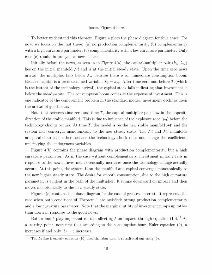
To better understand this theorem, Figure 4 plots the phase diagram for four cases. For

now, we focus on the first three: (a) no production complementarity, (b) complementarity

with a high curvature parameter, (c) complementarity with a low curvature parameter. Only

case (c) results in procyclical news shocks.

Initially before the news, as seen in in Figure 4(a), the capital-multiplier pair (kss, λss)

lies on the initial manifold M and is at the initial steady state. Upon the time zero news

arrival, the multiplier falls below λss because there is an immediate consumption boom.

Because capital is a predetermined variable, k0 = kss. After time zero and before T (which

is the instant of the technology arrival), the capital stock falls indicating that investment is

below the steady-state. The consumption boom comes at the expense of investment. This is

one indicator of the comovement problem in the standard model: investment declines upon

the arrival of good news.

Note that between time zero and time T , the capital-multiplier pair flow in the opposite

direction of the stable manifold. This is due to influence of the explosive root (µ2) before the

technology change occurs. At time T , the model is on the new stable manifold M′ and the

system then converges monotonically to the new steady-state. The M and M′ manifolds

are parallel to each other because the technology shock does not change the coefficients

multiplying the endogenous variables.

Figure 4(b) contains the phase diagram with production complementarity, but a high

curvature parameter. As in the case without complementarity, investment initially falls in

response to the news. Investment eventually increases once the technology change actually

occurs. At this point, the system is on the manifold and capital converges monotonically to

the new higher steady state. The desire for smooth consumption, due to the high curvature

parameter, is evident in the path of the multiplier. It jumps downward on impact and then

moves monotonically to the new steady state.

Figure 4(c) contains the phase diagram for the case of greatest interest. It represents the

case when both conditions of Theorem 1 are satisfied: strong production complementarity

and a low curvature parameter. Note that the marginal utility of investment jumps up rather

than down in response to the good news.

Both σ and δ play important roles in affecting λ on impact, through equation (10).17 As

a starting point, note first that according to the consumption-hours Euler equation (9), n

increases if and only if i− c increases.

17The L2 line is exactly equation (10) once the labor term is substituted out using (9).

15

Next, rewriting equation (10), we have:

λ︸︷︷︸MUI

= (v − 1) (i− c)︸︷︷︸priceI

+

(−σc− (1− σ) (1− α)

(1− sI)n

)︸︷︷︸

MUC

(22)

First, a good news shock that causes hours to rise is accompanied by an increase in the price

of investment (in units of consumption) when v > 1. This works to raise the marginal utility

of investment. Next, consumption also rises if the news shock is procyclical. The increases in

c causes the marginal utility of consumption to fall, which offsets the price effect on λ. This

effect is dampened when σ is close to zero. This is a straightforward channel operating in the

standard neoclassical model.18 Intuitively, when σ is close to zero the timing of investment

is governed by production efficiency concerns and not a desire to smooth consumption.

Finally, n appears in the MUC term because consumption and hours are non-separable in

the utility function. σ plays a different role in the term pre-multiplying n. Here, it effects the

degree of complementarity between n and c in preferences. If σ = 1, preferences are separable

and the n term drops out. If σ < 1, then leisure and consumption are complements, which

puts downward pressure on λ. It must be the case that the effect of σ on c dominates its

effect on n.

Thus, a low σ (through a dampened consumption effect) and the production complemen-

tarity lead to an overall increase in the shadow value of investment. This makes the return

to forgoing leisure in order to produce the investment good high.

Although investment jumps up at time zero, the new steady state must involve k′ss > kss

and λ′ss < λss. This occurs in case (c) because the new manifold eventually crosses into the

fourth quadrant of the phase space.

It is important to note that the conditions of Theorem 1 are independent of the value

of T . As a result, the model preserves the ability to generate procyclical comovements in

response to traditional time zero unanticipated shocks and news shocks that change the

level of technology for any time T in the future. Many models that can generate procyclical

comovements in response to news shocks are sensitive to the value T .

In addition to providing both the necessary and sufficient conditions for solving the news

shock puzzle, Theorem 1 provides insight into understanding how news shocks work. We

present our understanding via the following observation.

18If consumption and hours were separable, then σ is simply the inverse of the intertemporal elasticity ofsubstitution of consumption.

16

Main Observation A variant of the neoclassical model will exhibit procyclical technology

news shocks if it has one or more features that ensures:

I. consumption does not crowd out investment, or vice versa, and

II. the benefit to forgoing leisure is sufficiently strong.


Figure 5 plots how the critical value of the utility curvature parameter, σ∗, changes with

the capital share in production and the depreciation rate.19

As the capital share increases, the critical value of the utility curvature parameter in-

creases. This is because, as the capital share rises, the benefit to building capital increases,

inducing the planner to forgo leisure in order to produce investment. This greater willingness

to forgo leisure implies the model can support procyclical news shocks with less reliance on

low curvature in utility.

Next, consider the depreciation rate. As δ falls, the capital produced via investment in

response to the news will have suffered less depreciation by the time that technology increase

is realized. Thus, the planner is more willing to forgo leisure in order to produce investment.

Once again, this greater willingness to forgo leisure implies the model can support procyclical

news shocks with less reliance on low curvature in utility.

More formally, for the depreciation rate near zero, the second condition for a model to

exhibit procyclical news shocks simplifies dramatically.

Lemma 6. For δ sufficiently close to zero, the model exhibits procyclical news shocks if

υ > υ∗ and σ < 1.

Next, we plot the impulse responses for a specific model parameterization. Our model

calibration meets the two conditions: υ > υ∗ and σ < σ∗. First, υ = 1.8. Vall’es [35] finds

that υ = 1.8 best matches the estimated responses of investment to various shocks. Sims

[30] uses a similar F (C, I) function and chooses υ = 3.

The value of σ in our baseline calibration is 0.5, which implies less curvature than the oft-

used 1.0 (i.e. log utility). However, σ = 0.5 is within the range of some empirical estimates

19Remember σ < σ∗ supports procyclical news shocks. Holding labor fixed, σ is the inverse of theintertemporal elasticity of substitution. Thus a larger σ corresponds to greater curvature in the utilityfunction

17

(e.g. Beaudry & Wincoop [9], Vissing-Jorgensen & Attanasio [36] and Mulligan [26]). In

Section 4, we consider modifications of the production complementarity model that allow

for greater curvature in the utility function. The remaining parameters are less crucial and

entirely in line with existing research. All parameters are reported in Table 1.

[Insert Table 1 here]


The impulse responses are given in Figure 6. At time zero, capital is at the initial steady

state and agents receive news of an expected one-percent permanent increase in technology

that will arrive at T = 4. Examining panels (b), (c) and (d), we see that consumption,

hours and investment all increase on impact. Moreover, as our phase diagram and theorem

dictate, the shadow value of investment λ increases upon the arrival of the news (see panel

(f)).

The response of consumption, seen in panel (b), is positive but nearly zero. This may

be viewed as a deficiency of the model, although we note that non-durable consumption,

the closest analogue in actual data to consumption in our model, contributes very little

to empirical business cycles. In Section 4, we examine how adding various features to the

baseline production complementarity model can affect the impulse responses quantitatively.

3 Procyclical News Shocks via a Positive Labor Exter-

nality

This section modifies the preference side of the growth model as a way to sustain procyclical

news shocks. Specifically, we replace the momentary utility function in equation (4) with:

W(C,N, N

)= (1− σ)−1 [C exp

(−NN−γN

)]1−σwhere 0 < γN < 1 and N is the average economy-wide labor input.20 Thus, there is an

external effect of employment on utility. In particular, the marginal disutility of labor falls

as average labor rises. From an individual’s perspective, he would prefer to work additional

20To characterize the resource allocation in the presence of the externality, we have the social plannertake the time path of N as given when choosing the time paths of (C, I,K,N). Thus, we are studying aconstrained optimal plan. It is straightforward to show that this allocation is the same as what would obtainin a competitive equilibrium with the externality.

18

hours when others are working. In turn, the labor externality will act, from the household

perspective, similarly to a preference shock that shifts out labor supply. This mechanism

will ensure a low relative cost of forgoing leisure.

Also, we add investment adjustment costs by replacing (3) with

K = I − δK − ψI2

(1− I

δK

)2

I, (23)

In absence of adjustment costs (or an alternative appropriate mechanism), no stable solu-

tion exists at low values of σ. With the employment externality, production complementarity

is not necessary to support procyclical news shocks; as such, we set ν = 1.

The log-linearized equations that characterize a solution to the constrained planner’s

problem are now:

n =sI

1− γN(i− c) (24)

λ︸︷︷︸MUI

= ψI (i− k)︸︷︷︸priceI

+ (−σc− zn)︸︷︷︸MUC

(25)

λ = − (ρ+ δ) [(1− sI) (c− i) + i− k] + ρψI (i− k) (26)

as well as the resource constraints given by equations (12) and (13).

The term γN only appears in (24), the consumption-labor Euler equation.21and the ad-

dition of investment adjustment costs only alters equations (25) and (26).

We can substitute (24) into (12) to get a new consumption-investment production frontier

(new L1 line): (1− φLEI

)c+ φLEI i = αk + (1− α) a (27)

Here, φLEI =(

1− 1−α1−γN

)sI . In this model, L1 is upward sloping if φLEI < 0. This require-

ment, which simplifies to γN > α, is necessary and sufficient for comovement (although not

necessarily procyclical) in response to a news shock.


investment and hours comove at time zero if and only if γN > γ∗N = α.

21In fact, if one were to replace 1/ (1− γN ) with the value ν on the left-hand side, the equation would beidentical to (9) from the production complementarity model.

19

Lemma 7 is the labor externality counterpart to Lemma 1 for the production comple-

mentarity model.

The steps in characterizing the allocation under labor externalities are very similar to

those (previously done) under production complementarities. Two of the five equations,

as noted above, are identical across the two cases. The remaining three equations contain

nearly the same endogenous variables as in the previous model. Differences between the two

sets of preferences are limited to the coefficients multiplying the endogenous variables. As

such, we can apply the previous technique to this model.

The optimal solution satisfies the following conditions: 22

x = τLEx,k k + τLEx,λ λ+ τLEx,a a for x = c, i, n

[k

λ

]= ΓLE

[k

λ

]+ bLEa (28)

As mentioned previously for a model with labor externalities there exists no stable dy-

namic solution for low values of σ. The addition of investment adjustment costs alleviates

this problem. The next lemma holding fixed all other parameter values gives the mini-

mum value of ψI , the investment adjustment cost parameter, under which a stable dynamic

solution exists.


that γN > γ∗N . Then a stable solution to equation (28) exists if

ψI > ψ+I = −γ

LEI + φLEI σ

1− φLEI


that γN > γ∗N and ψI > ψ+I . λ(0) > 0 if and only if ψI > ψ∗I . where, ψ∗I solves equality

µLE2 =ΓLEλ,λb

LEk,a − ΓLEk,λb

LEλ,a

bLEk,a

and µLE2 = µLE2 (ψI) is the positive eigenvalue of ΓLE.

22The explicit formulas for τLE·,· , bLE and ΓLE are given in Appendix B.

20

Theorem 2. The labor externality model exhibits procyclical technology news shock if: γN >

γ∗N and ψI > Max{ψ+I , ψ

∗I

}.

Here is the intuition and relation to our main observation. As labor increases, the

marginal product of labor falls, which reduces the incentive to work. Without an exter-

nal effect, the marginal disutility of labor is increasing in labor. Thus, these two effects work

in the same direction. On the other hand, with the external effect, in a symmetric equi-

librium, the effective marginal disutility of labor is falling in labor. If the labor externality,

measured by γN , has a stronger positive labor supply effect than the negative diminishing

returns to labor demand effect, measured by 1 − α, then the employment increase will be

sufficiently large to support both a consumption and investment increase.23 Thus, the labor

externality mechanism achieves Condition I.

Next, equation (25) is critical for ensuring that the marginal utility of investment rises

on impact. The intuition here is identical to that of the production complementarity model

with one difference. In the current model, the price of investment (see the right-hand side

of equation (25)) increases because of investment adjustment costs term, ψI (i− k). In

the production complementarity model, the price of investment (see the right-hand side of

equation (22)) increased because of the production complementarity term, v (i− c). The

adjustment cost mechanism achieves Condition II.

Although the labor externality model has a different mechanism than the production

complementarity model, the relevant diagrams for the two models are identical. Figure

4(c) is the correct phase diagram for the new model; Figures 2 and 3 illustrate the static

relationships for the new model.

Next, we plot the impulse responses for a specific model parameterization. Our model

calibration meets the requirement γN > α and the two conditions on ψI . We set γN =

0.332, ψI = 20 and σ = 1. All parameters values are reported in Table 1.

The values of σ and ψI are in line with those of existing research. On the other hand, γN

is chosen somewhat arbitrarily because existing research provides no guidance for choosing

its value. This parameter choice is motivated by our desire to demonstrate one mechanism

capable of supporting procyclical news shocks.


23For parameter pairs (γN , α) that satisfy the comovement condition, note that there does not exist aninterior solution to the first-best resource allocation. With γN > 0, the social marginal disutility of laboris declining, rather than rising, as labor increases. With γN > α, this decline occurs more rapidly than theincrease in marginal cost associated with diminishing returns.

21

The impulse responses are given in Figure 7. Consumption, hours, investment as well

the shadow value of investment all increase upon the arrival of the news. Quantitatively,

we view the results as disappointing. Each of the three main variables is nearly acyclical in

response to the positive news.24

4 Quantitative Issues and Calibration Issues

Section 2 established that adding production complementarity to the neoclassical growth

model was sufficient to support procyclical news shocks. The mechanism, by itself, has two

potential drawbacks: the resulting consumption boom is miniscule and it requires low curva-

ture in the utility function. The former drawback is also present in the preference-externality

model. This section restricts attention to the production complementarity model and shows

how either changing preferences or adding investment adjustment costs can mitigate these

difficulties.

Greenwood-Hercowitz-Huffman Preferences

Suppose we replace the King, Plosser and Rebello preferences [23] (hereafter KPR), used ear-

lier in this paper, with those of Greenwood, Hercowitz and Huffman [16], GHH preferences.

The instantaneous utility function becomes

V (C,N) =

(C − ξN

1+ψ

1 + ψ

)1−ω

/ (1− ω)

where ω, ξ, ψ > 0. The set-up is otherwise identical to the production-complementarity

model.

The critical feature of these preferences is that the marginal disutility of labor is falling in

consumption. Recall that, in absence of a low σ under the KPR preferences, it was optimal

for the planner to delay the hours boom until the new technology arrives. Under GHH

preferences, the marginal disutility of work is falling in consumption; as such, there is an

preference-driven incentive to work more during a consumption boom.

The log-linearized conditions for an optimum consists of five equations, three of which are

identical to the baseline production-complementarity model.25 The first equation (that does

24It should be noted that in our simulation the marginal product of labor, a measure of real wage, falls inresponse to a positive news shock, however, similar to the other variables the quantitative response is nearlyacyclical.

25The unchanged equations are (11), (12), and (13).

22

change) is the intratemporal consumption-hours Euler condition. Under GHH preferences,

it is:

n = vsI (i− c) + c (29)

For comparison, we restate the corresponding equation for the baseline preferences:

n = vsI (i− c)

The production-complementarity effect, reflected by the vsI (i− c) term, is present in

both equations. GHH preferences, additionally, imply that the planner works more hours

when consumption is high. This augments the model’s ability to achieve Condition I.

The second equation (that does change) is the consumption-investment Euler condition.

Under GHH preferences, it is 26

λ = (ν − 1) (i− c) +1

1− sn1+ψ

[−ωc+ ωsnn]︸︷︷︸MUC

(30)

For the baseline preferences, we have

λ = (v − 1) (i− c) +

[−σc− (1− σ)

(1− α1− sI

)n

]︸︷︷︸

MUC

Recall that in order for comovement to be procyclical with respect to positive news, λ must

increase upon arrival of the news. This is an implication of our Condition II. Under the

baseline preferences, we showed that this was qualitatively possible if v was sufficiently

large and σ was sufficiently close to zero; however, quantitatively the consumption boom

was nearly very small. Examining the KPR preferences, one sees that λ is decreasing in

consumption. Roughly speaking, the planner attempts to allocate output to consumption

and investment to equalize their marginal benefit. If consumption rises too much, then the

marginal utility of consumption, MUc, will fall too much. In turn, the marginal utility of

investment would also have to fall.

GHH preferences help support an increase in λ in response to positive news. This is

because, while MUc is falling in consumption, it is rising in hours worked for any ω. Since

labor and consumption comove, this leads to an offsetting effect on MUc.

26Here sn = (1−α)1−sI

23

The steps in characterizing the optimal allocation under GHH preferences are very similar

to those described previously. Three of the five equations, as noted above, are identical across

the two cases. The remaining two equations, (29) and (30), for the GHH-preferences case,

contain the same endogenous variables as in the KPR case. Differences between the two

preference assumptions are limited to the coefficients multiplying the endogenous variables.

As such, we can apply the previous technique.

The optimal solution satisfies the following conditions: 27

x = τGHHx,k k + τGHHx,λ λ+ τGHHx,a a for x = c, i, n[k

λ

]= ΓGHH

[k

λ

]+ bGHHa


Next, we examine the quantitative implications of applying GHH preferences. The three

new model parameters are set at ω = 0.5, ψ = 0.01, and the scale parameter ξ = 6.96 to

match a steady state value of labor hour, N = 0.3. We calibrate the remaining parameters

at the values used in Section 2. Figure 8 plots the impulse responses. When compared to

the earlier models the magnitude of the initial responses are larger.

Investment Adjustment Costs

Condition II to generate procyclical news shocks requires a model feature that will ensure

the benefit to forgoing leisure sufficiently outweighs the cost. Parameterizing our model with

a high intertemporal elasticity of substitution led to us satisfying this condition in our basic

production-based model. Further analysis of the marginal effect of other parameters in that

model showed that increasing the marginal returns to investment, either by increasing the

capital share in production or lowering the depreciation rate, also led to an increase in the

benefit to forgoing leisure, albeit not large enough 28. The natural extension thus would

be to include a feature that generates a very high return to investment, such as investment

adjustment costs.

We make one modification to the baseline production-complementarity model. We intro-

duce investment adjustment costs by replacing (3) with (23).

27The explicit formulas for τG·,· and ΓG are given in Appendix B. This appendix also contains the conditionson the underlying parameters (α, ω, ρ, δ, ν, ξ) required for the model to exhibit procyclical news shocks.

28We still need higher than normal values of the intertemporal elasticity of substitution

24

This addition alter equations (10) and (11) in our log-linearized system by adding a new

term:

λ = (υ − 1) (i− c) + ψI (i− k)︸︷︷︸priceI

+

(−σc− (1− σ)

(1− α1− sI

)n

)(31)

λ = − (ρ+ δ) [υ (1− sI) (c− i) + i− k] + ρψI (i− k) (32)

The remaining three equations are unchanged.

Equation (31) gives us the optimal consumption-investment decision. It is identical to

the baseline production-complementarity model except there is an additional component to

the price of investment, ψI (i− k). This component is due to the investment adjustment

costs, is increasing in i and works to increase λ. The phase diagrams in Section 2 showed

why an increase in λ upon arrival of the news is required in order that a model support

procyclical comovement. Adjustment costs help ensure that increase in λ, and, therefore,

Condition II.

Equation (32) is the intertemporal consumption Euler equation. The sole difference in

this equation from the baseline production-complementarity model is that the rate of change

in the marginal utility of investment reflects the investment adjustment cost.

Next, consider the impact of adjustment costs on Condition I. Even though the addition of

investment adjustment costs alters equation (10), and thus the static system, it can be shown

that the Lemmas 1 through 4 still hold. The L1 line, equation (15), remains the same, and

while the magnitude of the slope of L2 changes quantitatively, there is no qualitative change.

Figures 2(b) and 3 still reflect (qualitatively) the static and required dynamic relationship

in the adjustment cost model.

With investment adjustment costs the dynamic analysis is slightly altered. Lemma 5, and

thus Theorem 1, now place a different parameter restriction required to generate a positive

λ (0). Most importantly the restriction on the critical value of σ is relaxed. High investment

adjustment costs lead to an increase in the returns to investment, which in turn leads to

more capital, which further in turn leads to an increase in the benefit of supplying labor and

forgoing leisure. Finally, the dynamic analysis in the (k, λ) space is qualitatively still given

by Figure 4.

In figure 8 we examine the quantitative implications of adding investment adjustment

costs. We set σ = 1 and ψI = 10, the remaining parameter values remain the same as before

(see table 1). The addition of investment adjustment costs lets us generate procyclical news

25

shocks with higher curvature in utility.

5 Forward-Compatible Investment

One observation, thus far, has been that in order to generate procyclical news shocks we re-

quire a feature or features that increases λ(0), which is an alternative expression of Condition

II. In this section, we describe how this can be achieved by introducing forward-compatible

investment. Physical investment is forward-compatible if additions to the capital made be-

tween the arrival of the news and the actual technology increase are particularly well-suited

to the future technology. For example, if an IT firm is laying down fiber optic cables and it

knows a new, better standard will be in effect in a year then it may be able to ensure that

the fiber optic cables currently being installed can take advantage of the new standard. This

will mean that at least part of the investment done in the preparatory phase (t ∈ [0, T )) will

be able to have an advantage of the new technology improvement once time T arrives. 29

The Model

Suppose that at time zero, news arrives of a future investment-specific technology shock.30

The technology increase will arrive at T > 0 and will be permanent:

Q (t) =

{Q for t ∈ [0, T )

Q = 1.01× Q t ≥ T(33)

We shall refer to time between zero and T as the preparatory phase.

This shock appears in the capital law of motion:

K (t) = Q (t) I (t)− δK (t) +(K (t)− e−δT K

)P(Q, t, T, ε

)(34)

where K is the initial capital stock, which we assume is at the steady-state consistent with

Q.

Here q can be interpreted as the level of technology embodied in the capital created at

a point in time. The function P represents the idea that capital might embody additional

29Baron & Schmidt [1] provide evidence for this mechanism. They document how the adoption of newstandards both gives a signal about future technological change - ”news shocks” - and subsequently resultsin slow diffusion of technology.

30Investment-specific technology shocks by themselves cannot generate news-driven procyclical businesscycles, established in Beaudry and Portier [7].

26

technology that does not become useful until a future date - forward compatibility of capital

with future technology.31

The right-hand side of (34) decomposes the time derivative of capital into three terms.

The first term is the contribution of investment multiplied by the current efficiency of invest-

ment. The second is the capital lost due to depreciation. The last term embodies the model’s

key assumption. It is the multiple of two functions. The first function is K (t) − e−δT K,

representing the investment accumulated during the preparatory phase that has not depre-

ciated. For convenience, define K (t) = K (t) − e−δT K. The second function, P (Q, t, T, ε),

is a positive technology shock. It will be constructed so that it permanently increases the

productivity of investment made during the preparatory phase. Thus, investment made after

the arrival of news will be forward-compatible with the yet-to-arrive technology.

This second function will be non-zero only in a small neighborhood of T . Thus, this

positive shock will not come online until time T . The contribution of the third term in (34)

will only apply to K (T ). We refer to K (T ) as partially-adapted capital. We plot the log

deviations of the functions Q and P in Figure 9.


P depends on t because the forward-compatible effect is only operative for a certain

interval of time. The term ε is a small positive number. It will define the neighborhood

(of the time interval) in which the “forward-compatibility”shock occurs. Mathematically,

P (Q, t, T, ε) 6= 0 only if t ∈ [T, T + ε]. A technical detail necessitates ε.32 Later, we will

drive ε to zero at the appropriate rate. We choose a particular form for P to aid calibration:

P(Q, t, T, ε

)=

{0 for t ∈ [0, T ) ∪ (T + ε,∞)τQ

(1−e−ε)Q t ∈ [T, T + ε]

For notational simplicity, we will sometimes use Pε (t) and suppress the function’s dependence

on Q and T .

A positive investment-specific technology shock is isomorphic to a positive neutral tech-

nology shock combined with a capital depreciation shock. Forward compatability, in the face

of an investment-specific news shock, mitigates the “capital depreciation” shock component.

31The relationship between investment-specific technology and capital embodiment is discussed in Green-wood, Hercowitz and Huffman [16].

32If P were positive and finite only at one instant, then P will have zero effect on the capital. Instead,as we let ε approach zero, the P will become infinite at the instant T and cause K to jump upward. Thistechnical detail is not needed in a discrete time model.

27

That is, capital put in place following the news will not depreciate to the same degree as the

already in-place capital. Thus, forward compatability, by itself, boosts the relative benefit

to forgoing leisure to produce investment upon the news arrival.

Production of consumption occurs according to equations (1) and (2); that is, there is

production complementarity between consumption and investment.33 The utility function is

(4), which is taken from the baseline model of Section 2.

The Planning Problem and Its Solution

The social planner chooses C, I, K and N to maximize U subject to (1), (2) and (34),

taking as given the initial condition K (0) and time path of technology. The current value

Hamiltonian for the problem is:

H = (1− σ)−1C1−σ exp [− (1− σ)N ] + Λ (QI − δK + PεK) + Φ(KαN1−α − F (C, I)

)The log-linearized system that solves this Hamiltonian is given by five equations.34 Two

equations, (9) and (12), are identical to those from the baseline production complementarity

model. These are the consumption-hours Euler equation and the production function. The

three new equations are:

λ = (υ − 1) (i− c) + (−σc− zν)− q (35)

λ = − (ρ+ δ) [v (1− sI) c+ q + i− k]− pε (36)

k = δ (q + i− k) + (1− e−δT )pε (37)

Equation (35) ensures an efficient consumption-investment split. It is identical to the cor-

responding equation from the baseline production complementarity except for the final term

on the right-hand side, −q. This is a relative price effect because technology is investment-

specific. Before time T , however, q (t) = 0 because the technology improvement has not yet

arrived.

Equation (36) is the intertemporal consumption Euler equation. It differs from the neo-

classical model in two ways. First, λ is not simply the derivative of the marginal utility of

consumption. There is an additional relative price effect because of the convex production

frontier. Second, λ jumps down at T as a result of pε, that is in the limit as ε→ 0.

33We assume that At = 1, since technology improvements are only investment specific in this model.34The non-linear first-order conditions are presented in Appendix B.

28

Equation (37) is the law of motion for capital. On the right-hand side, the first term

is standard and the second reflects an increase in capital at time T . This occurs when

the forward-compatible capital built during the preparatory phase becomes utilized with

the new technology. Recall that pε is positive, and otherwise zero, only in a neighborhood

of T . Below, we take the limit as ε → 0. Then, pε becomes ”infinite at an instant,”

causing an upward jump in the capital stock. The optimal solution also satisfies a standard

transversality condition and an initial condition on capital.

Recall that, in order to support procyclical news shocks, a model must have mechanism(s)

that ensure: (I) consumption does not crowd out investment, and (II) a sufficiently large

return to forgoing leisure.

Production complementarity is sufficient to ensure Condition I due to the derivations in

the benchmark production complementarity model. Lemma 1 holds for this model.

Following the same techniques as for the benchmark production complementarity model35, we have expressions for the jump variables (consumption, investment and hours) as

functions of the state variables.

x = τFCx,k k + τFCx,λ λ+ τFCx,q q for x = c, i, n (38)

Substituting (38) into the k and λ equations, (36) and (37), we have:36

[λ (t)

k (t)

]= ΓFC

[λ (t)

k (t)

]+ bFCq q (t) + bFCp p (q, t, T, ε) (39)

Solving the differential equation (39), the time-paths of (k, λ) are:37

k (t) =

Γk,λλ(0)

µ1−µ2eµ1t +

Γk,λλ(0)


Γk,λλ(0)

µ1−µ2eµ1t +

Γk,λbλ,q−Γλ,λbk,qµ1µ2

+Γk,λ(bλ,q+τµ1bλ,pε)+(µ1−Γλ,λ)(bk,q+τµ1bk,pε)

µ1(µ1−µ2)eµ1(t−T ) t ≥ T

(40)

λ (t) =

(µ1−Γk,k)λ(0)

µ1−µ2eµ1t +

(µ2−Γk,k)λ(0)


(µ1−Γk,k)λ(0)

µ1−µ2eµ1t +

Γλ,kbk,q−Γk,kbλ,qµ1µ2

+Γλ,k(bk,q+τµ1bk,pε)+(µ1−Γk,k)(bλ,q+τµ1bλ,pε)

µ1(µ1−µ2)eµ1(t−T ) t ≥ T

(41)

where µ1 and µ2 are the eigenvalues of the ΓFC matrix.38

35Details can be found in Appendix B.36The explicit formulas for τFC·,· ,Γ

FC , bFCq and bFCp are given in Appendix B.37Appendix B contains the derivation of (40) and (41)38In the above expressions and the expression below, we suppress the superscript FC from several variables

29

The above solution has one undetermined variable λ(0). We seek a path for (λ, k) that

is not explosive. We choose λ(0) such that the explosive root µ2 does not determine the

evolution of the system for t > T ; otherwise, the path would be explosive. This restriction

on λ(0) is:

Γk,λλ(0) + (µ2 − Γλ,λ) k(0)

(µ2 − µ1)= −Γk,λ (bλ,q + τµ2bλ,pε) + (µ2 − Γλ,λ) (bk,q + τµ2bk,pε)

µ2 (µ2 − µ1)e−µ2T

Next, we provide a theorem concerning procyclical news shocks in the forward-compatibility

model.39

Theorem 3. The forward-compatible investment model exhibits procyclical technology news

shocks if and only if υ (1− α) > 1 and

τ >ΓFCk,λ b

FCλ,q +

(µFC2 − ΓFCλ,λ

)bFCk,q

ΓFCk,λµFC2 bFCλ,pε +

(µFC2 − ΓFCλ,λ

)µFC2 bFCk,pε

(42)

where µFC2 is the positive eigenvalue of ΓFC.

Let us understand this result: Theorem 3 requires that there is both sufficient comple-

mentarity in production (Condition I) and the new capital accumulated between time 0 and

T must be sufficiently forward compatible (Condition II).

Panel (d) of Figure 4 contains the phase diagram for the forward-compatibility model

when the conditions of Theorem 3 are satisfied. Before the news shock, the economy is at

its initial steady state (kss, λss). The initial capital stock is lower and the shadow value

of investment is larger than their long-run, post-shock counterparts (k′ss, λ′ss). M is the

pre-shock stable manifold and M′ is the corresponding manifold after time T .

At the instant of the news arrival, the shadow value of investment increases. This occurs

because new investment will be more productive relative to previous investment, albeit not

until time T . Capital does not jump instantaneously; however k (0) > 0. This shows that

investment increases in response to the shock—the first of three requirements for procyclical

news shocks. The reader should return to Figure 2(b) to see graphically that the second

requirement–that consumption rises–is satisfied. That figure shows that the increase in λ

to avoid notational clutter.39It should be noted that Lemmas 2-4 also hold for the forward compatible investment model.

30

results in higher consumption.40 The third requirement—that hours increase– holds because,

otherwise, both consumption and investment could not increase.

At instant T , the actual increase in investment specific technology occurs. All future

investment produces an additional one percent of capital. Moreover, because of forward

compatibility, investment made during the preparatory phase becomes τ percent more pro-

ductive. This latter effect causes the capital to jump up at T . This latter effect also causes

λ to jump down from T− to T+. When the capital stock jumps up, the shadow value of

investment, i.e. adding to that capital stock, declines in a discrete fashion. During the

preparatory phase, the explosive root is operative, causing λ to rise.

Next, at and after time T+, k and λ lie on the new stable manifoldM′. If (k (t) , λ (t)) did

not lie on M′ for t > T+, then the pair would diverge. Intuitively, going from T+ onward,

k and λ must be on the new manifold because technology has reached its new permanently

higher level.41

The dynamics of news shocks of every model in this paper are contained in Figure 4. All

models discussed in the paper, excluding the forward-compatible model, achieve λ(0) > 0

by causing the stable manifold to shift upwards. With the forward compatibility, this is not

necessary. We can maintain the stable manifold movements as in the standard neoclassical

model and yet generate procyclical news shocks by instead adding in a friction that results

in a discontinuity in the time path of the state and co-state variables. This allows a fair

amount of flexibility in adding other non-related frictions and still generating procyclical

news shocks.

Including a feature that adds a discontinuity to the state variable allows for richer dy-

namics and places fewer restrictions on the movements of the stable manifold vis-a-vis the

inclusion of other economic frictions.

Quantitative Analysis of the Forward-Compatibility Model

40The intuition for this effect is discussed early in the paper.41The partial forward-compatible assumption in this model is similar to the time-to-build assumption where

K (t) = Q (t) I (t− ξ)−δK (t) (here ξ gives a measure of how long it takes to build capital). It can be shownthat in a model with production complementarity and time-to-build if ξ > T then under certain plausiblecalibrations the model is able to generate procyclical technology news shocks. These models are howeverdistinct. The two key differences are: (i) under time-to-build investment made today doesn’t come onlineuntil ξ periods into the future, whereas; partially forward-compatible investment is available immediatelyafter it is created. (ii) under the partially forward-compatible assumption only part of the investment createdbefore the technology increase will experience an increase in efficiency when the actual technology increases,whereas; under time-to-build with ξ > T all the investment created before the technology increase willexperience an efficiency increase when the investment becomes available.

31

The only new parameter is τ , the degree of forward compatibility. This is clearly a difficult

parameter to calibrate. We set τ = 0.66, a little above the critical value of τ ≈ 0.5 to

demonstrate the models ability to generate procyclical news shocks. We can now also set

the utility curvature parameter to a higher value of σ = 1. The remaining parameters are

set at values used earlier in the paper.


Figure 10 plots the responses of key variables to a positive news shock. As seen in

panels (b)-(d), consumption, investment and hours all increase on impact upon the arrival

of the news. The three then increase smoothly until the beginning of quarter four. Then

technology actually increases; each of the three jumps upward because the output cost of

producing newly installed capital, 1/Q, falls.

Although we set T = 4 (i.e. one year) in our baseline calibration, the model can exhibit

procyclical news shows for much higher values of T . Holding all other parameters fixed at

their benchmark values calculations based on Theorem 3 imply that procyclical news shocks

obtain for any T < 21.3.

Next, the relative price of investment to consumption, seen in panel (e), rises on impact

due to production complementarities along with a larger increase in investment relative to

consumption in response to the news. Panel (f) shows that the shadow value of investment

also increases on impact.

With respect to existing research, we note that Floden [15] has a paper related to ours.

He constructs a two-period model that is capable of resolving the comovement puzzle using

variable capacity utilization and vintage capital. In his paper, news arrives in the initial

period and technology arrives in the second period. The news increases the efficiency of

investment made in the initial period toward producing capital in the second period, which

is similar to our forward-compatibility.

Value of the Firm

We are additionally interested in the value of the capital stock, which can be interpreted as

the value of the stock market in a typical decentralization of our social planner’s problem.

Our interest is partly empirical: using a VAR strategy, Beaudry and Portier [6] find that the

real value of the S&P500 is procyclical with respect to technology news shocks.


32

Figure 11 plots the value of the firm in each of our five model economies. For our first

four models the value of the firm rises in response to news.

Here is the intuition. Recall that the models presented in panel (a) and (c) all contain

production complementarities. The presence of production complementarities increase the

price of investment relative to consumption when the planner moves to increase investment in

response to a news shock. An increase in the price of investment raises the value of installed

capital. Investment adjustment costs, present in the models of panels (b) and (c), increase

the price of investment during the investment boom, thereby reinforcing the production

complementarity channel. Thus, the increased price of investment in all four models results

in an increase in the value of the capital stock.42

The dashed line in panel (d) plots the value of the capital stock with forward compatible

investment for our benchmark calibration. The value of the firm falls even though, as with

the models in panels (a) and (c), this model also contains production complementarities.

The reason that the firm’s value falls is, unlike the first three panels, the exogenous news in

(d) is regarding investment-specific technology, rather than neutral technology.

In the standard neoclassical model, a contemporaneous positive investment-specific tech-

nology shock causes the value of the firm to fall. Recall the value of the firm is simply the

value of its capital. Higher productivity in the capital producing sector depresses the price

of capital. Thus, the value of the firm’s existing capital must fall on impact. This channel

is operational for news about investment-specific technology as well.

These results suggest that models with neutral-technology, as opposed to investment-

specific technology, news shocks do have one advantage in terms of generating procyclical

stock prices.

6 Conclusion

In this paper, we have made the case that an analytic approach to understanding news

shocks in stochastic growth models is insightful. Up to a first-order approximation, we have

provided analytic solutions to five variants on the standard neoclassical model. In each case,

we have provided conditions under which the model exhibits procyclical news shocks. For

each, we have provided a plausible calibration and then examined the quantitative features

42We use the benchmark calibration in Table 1 to compute these impulse responses. In addition it can easilybe shown that for the production complementarity model, the labor externality model, and the investmentadjustment cost model of panels (a)-(c) the time 0 value of the firm will increase for all parameters underwhich those models exhibit procyclical news shocks.

33

of the model’s impulse response functions.

By examining several models, we have identified commonalities across their respective

mechanisms that generate resolutions of the news-shock comovement puzzle. In particular,

each model has a mechanism or mechanisms that ensure that consumption and investment

do not crowd each other out and that the relative benefit of forgoing leisure outweighs its

cost.

As a result of our analysis, we have further developed a view on what type of mechanisms

are best suited for achieving the above conditions. We contend that it is more reasonable

to attribute procyclical news shocks to production-based rather than preference-based com-

ponents. For example, GHH preferences help significantly boost the size of a consumption

boom in the production complementary model; however, using these preferences creates

other problems, not related to news shock. These include an absence of balanced growth

with respect to neutral technological change. On the other hand, the addition of production

complementarity, which has an interpretation as a two-sector neoclassical model, seems, in

our view, to be a plausible production-based mechanism.

34

Bibliography

[1] Baron, Justus, and Julia Schmidt, “Technological Standardization, Endogenous Produc-

tivity and Transitory Dynamics,” mimeo, Northwestern University, 2014.

[2] Barsky, Robert B., and Eric Sims, “News Shocks and Business Cycles,” Journal of Mon-

etary Economics, 58:273-289, 2011.

[3] Beaudry, Paul, Martial Dupaigne, and Franck Portier, “Modeling News-Driven Interna-

tional Business Cycles,” Review of Economic Dynamics, 14:72-91, 2011.

[4] Beaudry, Paul and Bernd Lucke, “Letting Different Views about Business Cycles Com-

pete,” NBER Macroeconomics Annual 2009, 24:413-455, 2010.

[5] Beaudry, Paul and Franck Portier, “An Exploration into Pigou’s Theory of Cycles,” Jour-

nal of Monetary Economics, 51:1183-1216, 2004.

[6] Beaudry, Paul and Franck Portier, “Stock Prices, News, and Economic Fluctuations,”

American Economic Review, 96:1293-1307, 2006.

[7] Beaudry, Paul and Franck Portier, “When Can Changes in Expectations Cause Business

Cycle Fluctuations in Neo-Classical Settings?,” Journal of Economic Theory, 135:458-477,

2007.

[8] Beaudry, Paul and Franck Portier, “News Driven Business Cycles: Insights and Chal-

lenges,” NBER Working Paper 19411, 2013.

[9] Beaudry, Paul, and Eric van Wincoop, “The Intertemporal Elasticity of Substitution: An

Exploration using a US Panel of State Data,” Economica, 63:495-512, 1996.

[10] Boyce, William E., and Richard C. DiPrima, Elementary Differential Equations and

Boundary Value Problems, John Wiley & Sons, New York, 1969.

[11] Campbell, John Y., “Inspecting the Mechanism: An Analytical Approach to the Stochas-

tic Growth Model,” Journal of Monetary Economics, 33:463-506, 1994.

35

[12] Chen, Kaiji, and Zheng Song, “Financial Frictions on Capital Allocation: A Transmis-

sion Mechanism of TFP Fluctuations,” Journal of Monetary Economics, forthcoming.

[13] Christiano, Lawrence, Cosmin Ilut, Roberto Motto, and Massimo Rostagno, “Monetary

Policy and Stock Market Boom-Bust Cycles,” Working Paper Series 955, European Central

Bank, 2008.

[14] Comin, Diego A., Mark Gertler, and Ana Maria Santacreu, “Technology Innovation

and Diffusion as Sources of Output and Asset Price Fluctuations,” Harvard Business School

Working Paper, 09-134, 2009.

[15] Floden, Martin, “Vintage Capital and Expectations Drive Business Cycles,” CEPR

working paper, 2007.

[16] Greenwood, Jeremy, Zvi Hercowitz, Gregory W. Huffman, “Investment, Capacity Uti-

lization, and the Real Business Cycle,” American Economic Review, 78:402-417, 1988.

[17] Gunn, Christopher, and Alok Johri, “News and Knowledge Capital,”Review of Economic

Dynamics, 14:92-101, 2011.

[18] Huffman, Gregory and Mark Wynne, “The Role of Intratemporal Adjustment Costs in

a Multisector Economy,” Journal of Monetary Economics, 43:317-350, 1999.

[19] Jaimovich, Nir, and Sergio Rebelo, “Can News About the Future Drive the Business

Cycle?,” American Economic Review, 99:1097-1118, 2009

[20] Judd, Kenneth, “An Alternative to Steady-State Comparisons in Perfect Foresight Mod-

els,” Economic Letters, 10:55-59, 1982.

[21] Judd, Kenneth, “Short-Run Analysis of Fiscal Policy in a Simple Perfect Foresight

Model,” Journal of Political Economy, 93:298-319, 1985.

[22] Khan, Hashmat and John Tsoukalas, “The Quantitative Importance of News Shocks in

36

an Estimated DSGE Model,” Journal of Money, Credit, and Banking, 44:1535-1561, 2012.

[23] King, Robert G., Charles I. Plosser and Sergio T. Rebelo, “Production, Growth and

Business Cycles I. The Basic Neoclassical Model,” Journal of Monetary Economics, 21:195-

232, 1988.

[24] Leeper, Eric M., Todd Walker, and Shu-Chun (Susan) Yang, “Foresight and Information

Flows,” Econometrica, 81:1115-1145, 2013.

[25] Lorenzoni, Guido, “News and Aggregate Demand Shocks,” Annual Review of Economics,

3:537-557, 2011.

[26] Mulligan, Casey, “Capital, Interest, and Aggregate Intertemporal Substitution,” NBER

Working Paper 9373, 2002.

[27] Nah, Seungho, “Financial Frictions, Intersectoral Adjustment Costs, and News-Driven

Business Cycles,” mimeo, The Ohio State University, 2009.

[28] Qureshi, Hammad, “News Shocks and Learning-by-Doing,” mimeo, The Ohio State Uni-

versity, 2009.

[29] Schmitt-Grohe, Stephanie and Martin Uribe, “What’s News in Business Cycles,” Econo-

metrica, 80:2733-2764, 2012.

[30] Sims, Christopher A., “Models and their Uses,”American Journal of Agricultural Eco-

nomics, 71:489-494, 1989.

[31] Tenenbaum, Morris and Harry Pollard, Ordinary Differential Equations, Dover, 1985.

[32] Tsai, Yi-Chan, “News Shocks and Costly Technology Adoption,” mimeo, The University

of Tokyo, 2009.

[33] Walentin, Karl “Expectation Driven Business Cycles with Limited Enforcement,” Sveriges

Riksbank Working Paper No. 229, 2012.

37

[34] Wang, Pengfei, “Understanding Expectation-Driven Fluctuations—A Labor Market Ap-

proach,” Journal of Money, Credit and Banking, 44:487-506, 2012.

[35] Vall’es, Javier, “Aggregate Investment in a Business Cycle Model with Adjustment

Costs,” Journal of Economic Dynamics and Control, 21:1181-1198, 1997.

[36] Vissing-Jorgensen, Annette, and Orazio P. Attanasio, “Stock Market Participation,

Intertemporal Substitution, and Risk Aversion,” American Economic Review, 93:383-391,

2003.

38

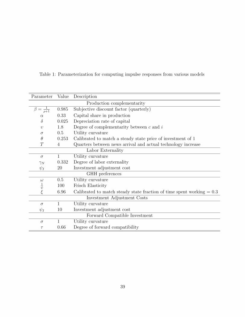
Table 1: Parameterization for computing impulse responses from various models

Parameter Value Description

Production complementarityβ = 1

ρ+10.985 Subjective discount factor (quarterly)

α 0.33 Capital share in productionδ 0.025 Depreciation rate of capitalυ 1.8 Degree of complementarity between c and iσ 0.5 Utility curvatureθ 0.253 Calibrated to match a steady state price of investment of 1T 4 Quarters between news arrival and actual technology increase

Labor Externalityσ 1 Utility curvatureγN 0.332 Degree of labor externalityψI 20 Investment adjustment cost

GHH preferencesω 0.5 Utility curvature1ψ

100 Frisch Elasticity

ξ 6.96 Calibrated to match steady state fraction of time spent working = 0.3Investment Adjustment Costs

σ 1 Utility curvatureψI 10 Investment adjustment cost

Forward Compatible Investmentσ 1 Utility curvatureτ 0.66 Degree of forward compatibility

39

Fig

ure

1:Im

puls

eR

esp

onse

toa

Pos

itiv

eN

ews

Shock

-B

asic

Neo

clas

sica

lM

odel

05

1015

0

0.2

0.4

0.6

0.81

(a)

Tec

hn

olo

gy

Log Deviations

05

1015

0

0.1

0.2

0.3

0.4

0.5

0.6

0.7

(b)

Co

nsu

mp

tio

n

05

1015

−6−4−20246(c

) In

vest

men

t

05

1015

−1.5−1

−0.50

0.51

(d)

Lab

or

Log Deviations

Per

iod

s0

510

15−1

−0.50

0.51

(e)

Pri

ce o

f In

vest

men

t

Per

iod

s0

510

15−0

.7

−0.6

−0.5

−0.4

−0.3

−0.2

−0.10

(f)

Sh

ado

w V

alu

e o

f In

vest

men

t

Per

iod

s

40

Fig

ure

2:L

1an

dL

2ini-c

Spac

e,an

dan

incr

ease

inth

em

argi

nal

uti

lity

ofin

vest

men

t(λ

)

i

c

(a) w

ithou

t pro

duct

ion

com

plem

enta

rity

L 1

L 2

prod

uctio

n

cons

umpt

ion

-inve

stm

ent

(b)

with

pro

duct

ion

com

plem

enta

rity

L'2

i

c

L 1L 2

prod

uctio

n

cons

umpt

ion

-inve

stm

ent

L'2

41

Fig

ure

3:L

1an

dL

2ini-c

Spac

e,an

dan

incr

ease

inb

oth

the

mar

ginal

uti

lity

ofin

vest

men

t(λ

)an

dca

pit

al(k

)

i

c

L 1 =

L 1'

L 2

prod

uctio

n

cons

umpt

ion

-inve

stm

ent

L 2'L 2''L 2'''

L 1''L 1'''

Tim

e 0

Tim

e T-

Ɛ

42

Figure 4: Phase diagrams in (k, λ) space for a positive news shock

k

λ

(a) Standard Production, σ =1

(k0,λ

0)

(kT,λ

T)

(kss

,λss

)

(k'ss

,λ'ss

)

M

M'

(c) Production Complementarities, Low σ

λ

k

(k0,λ

0)

(kT,λ

T)

(kss

,λss

) (k'ss

,λ'ss

)

M

M'

k

λ

(b) Production Complementarities, High σ

(k0,λ

0)(k

T,λ

T)

(kss

,λss

)

(k'ss

,λ'ss

)

M

M'

k

λ

(d) Production Complementarities, Partial Forward Compatibility

(k0,λ

0)

(kT -

,λT -

)

(kss

,λss

)

(k'ss

,λ'ss

)

M

M'

(kT+

,λT+

)

43

Fig

ure

5:C

riti

cal

Uti

lity

Curv

ature

(σ∗ )

vs.

Oth

erM

odel

Par

amet

ers

00.

20.

40.

60.

81

00.

050.

10.

150.

20.

250.4

0.5

0.6

0.7

0.8

0.91

Cap

ital

Sh

are

in P

rod

uct

ion

(α)

Dep

reci

atio

n R

ate

(δ)

Critical Utility Curvature (σ*)

44

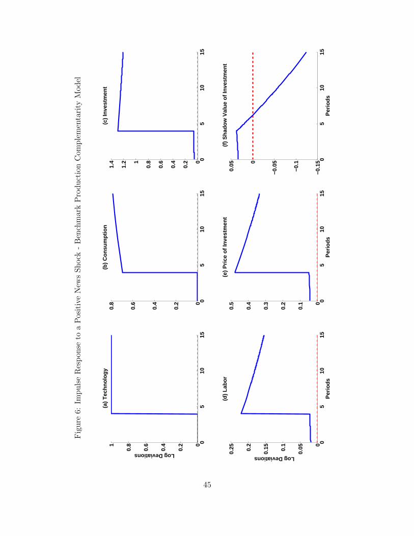
Fig

ure

6:Im

puls

eR

esp

onse

toa

Pos

itiv

eN

ews

Shock

-B

ench

mar

kP

roduct

ion

Com

ple

men

tari

tyM

odel

05

1015

0

0.2

0.4

0.6

0.81

(a)

Tec

hn

olo

gy

Log Deviations

05

1015

0

0.2

0.4

0.6

0.8

(b)

Co

nsu

mp

tio

n

05

1015

0

0.2

0.4

0.6

0.81

1.2

1.4

(c)

Inve

stm

ent

05

1015

0

0.050.

1

0.150.

2

0.25

(d)

Lab

or

Log Deviations

Per

iod

s0

510

150

0.1

0.2

0.3

0.4

0.5

(e)

Pri

ce o

f In

vest

men

t

Per

iod

s0

510

15−0

.15

−0.1

−0.0

50

0.05

(f)

Sh

ado

w V

alu

e o

f In

vest

men

t

Per

iod

s

45

Fig

ure

7:Im

puls

eR

esp

onse

toa

Pos

itiv

eN

ews

Shock

-L

abor

Exte

rnal

ity

Model

)

05

1015

0

0.2

0.4

0.6

0.81

(a)

Tec

hn

olo

gy

Log Deviations

05

1015

0

0.1

0.2

0.3

0.4

0.5

0.6

0.7

(b)

Co

nsu

mp

tio

n

05

1015

0

0.02

0.04

0.06

0.080.

1

0.12

(c)

Inve

stm

ent

05

1015

−0.3

−0.2

5

−0.2

−0.1

5

−0.1

−0.0

50

0.05

(d)

Lab

or

Log Deviations

Per

iod

s0

510

150

0.51

1.5

(e)

Pri

ce o

f In

vest

men

t

Per

iod

s0

510

150

0.2

0.4

0.6

0.81

(f)

Sh

ado

w V

alu

e o

f In

vest

men

t

Per

iod

s

46

Fig

ure

8:Im

puls

eR

esp

onse

toa

Pos

itiv

eN

ews

Shock

-V

aria

nts

onth

eP

roduct

ion

Com

ple

men

tari

tyM

odel

:G

HH

Pre

fere

nce

san

dIn

vest

men

tA

dju

stm

ent

Cos

ts

05

1015

0

0.2

0.4

0.6

0.81

Log Deviations

(a)

Tec

hn

olo

gy

GH

H P

refe

ren

ces

Inve

stm

ent

Ad

just

men

t. C

ost

s

05

1015

0

0.51

1.52

2.53

3.5

(b)

Co

nsu

mp

tio

n

05

1015

0123456(c

) In

vest

men

t

05

1015

−1012345(d

) L

abo

r

Log Deviations

Per

iod

s0

510

150

0.51

1.52

(e)

Pri

ce o

f In

vest

men

t

Per

iod

s0

510

150

0.51

1.52

2.5

(f)

Sh

ado

w V

alu

e o

f In

vest

men

t

Per

iod

s

47

Figure 9: Efficiency of Different Types of Capital

0 T T+ε t

pε(t)

0 T T+ε t

q(t)1

(a) capital efficiency of post-T investment

(b) change in capital efficiency of investment (done in preparatory phase)

τ/(1-e-ε)

48

Fig

ure

10:

Impuls

eR

esp

onse

toa

Pos

itiv

eN

ews

Shock

-F

orw

ard

Com

pat

ible

Inve

stm

ent

05

1015

0

0.2

0.4

0.6

0.81(a

) T

ech

no

log

y (I

nve

stm

ent

Sp

ecif

ic)

Log Deviations

05

1015

0

0.050.

1

0.150.

2(b

) C

on

sum

pti

on

05

1015

0

0.2

0.4

0.6

0.8

(c)

Inve

stm

ent

05

1015

0

0.050.

1

0.150.

2

0.25

(d)

Lab

or

Log Deviations

Per

iod

s0

510

15−0

.8

−0.6

−0.4

−0.20

0.2

(e)

Pri

ce o

f In

vest

men

t

Per

iod

s0

510

15−0

.8

−0.6

−0.4

−0.20

0.2

(f)

Sh

ado

w V

alu

e o

f In

vest

men

t

Per

iod

s

49

Fig

ure

11:

Impuls

eR

esp

onse

toa

Pos

itiv

eN

ews

Shock

-V

alue

ofth

eF

irm

05

1015

0

0.2

0.4

0.6

0.8

(a)

Pro

du

ctio

n C

om

ple

men

tari

ties

(N

eutr

al T

ech

no

log

y S

ho

ck)

Log Deviations

05

1015

0

0.51

1.5

(b)

Lab

or

Ext

ern

alit

ies

(Neu

tral

Tec

hn

olo

gy

Sh

ock

)

05

1015

0

0.51

1.52

2.53

Per

iod

s

Log Deviations

(c)

GH

H P

refe

ren

ces

& In

vest

men

t A

dju

stm

ent

Co

sts

(N

eutr

al T

ech

no

log

y S

ho

ck)

GH

H P

refe

ren

ces

Inve

stm

ent

Ad

just

men

t C

ost

s

05

1015

−0.5

−0.4

−0.3

−0.2

−0.10

0.1(d

) F

orw

ard

Co

mp

atib

ility

(In

vest

men

t−S

pec

ific

Tec

hn

olo

gy

Sh

ock

)

Per

iod

s

50

A Lemmas and Theorems

Proof of Lemma 1. Substituting (9) into (12):

αk + (1− α) a = (1− (1− υ (1− α)) sI) c+ (1− υ (1− α)) sIi

=(1− φPCI

)c+ φPCI i (A.1)

Here φPCI = (1− υ (1− α)) sI .

k(0) = 0 and a(0) = 0, therefore (A.1) can be written as:

0 =(1− φPCI

)c(0) + φPCI i(0) (A.2)

First, if υ (1− α) > 1, then φPCI < 0 &(1− φPCI

)> 0 . Therefore, if υ (1− α) > 1 and c(0)

increases then for (A.2) to hold i(0) must also increase.

Further, if υ (1− α) > 1, then(1− φPCI

)=(−φPCI + 1

)> −φI . Therefore, if c(0)

increases, then for (A.2) to hold i(0) must increase by a larger magnitude than c(0), this

implies (i(0)− c(0)) increases when c(0) increases, which in turn due to (9) implies that n(0)

must increase.

Therefore, if υ (1− α) > 1, then consumption, investment, and hours will comove at time

zero.

Second, if υ (1− α) < 1, then φPCI ∈ (0, 1) and(1− φPCI

)> 0. Therefore, if c(0) increases

then for (A.2) to hold i(0) must decrease. Therefore, if υ (1− α) < 1, then consumption,

investment and hours will not comove at time zero.


γPCI i−(σ + γPCI

)c = λ (A.3)

Here γPCI = (υ − 1)− (υ (1− α) (1− σ) sI) / (1− sI).

Further, substituting (A.1) into (A.3) and solving for c at time 0 leads to:

c(0) =−φPCI

γPCI + φPCI σλ(0) (A.4)

51

First, from the proof of lemma 1 we know that −φPCI > 0 if υ (1− α) > 1. Also, γPCI +

φPCI σ > 0 if υ (1− α) > 1.43 From equation (A.4) if λ(0) > 0 then c(0) will increase. If

c(0) > 0 then from the proof of lemma 1 we know that both i(0) and n(0) will also increase.

As a result, if υ (1− α) > 1 and λ(0) > 0, then consumption, investment, and labor

hours will comove procyclically at time zero in response to a news shock about technology

in time T > 0.

Second, by Lemma 1 we also know that if υ (1− α) < 1 and λ(0) > 0, then consumption

and investment will not comove at time zero.

Proof of Lemma 3. Solving (A.1) and (A.3) simultaneously for the values of c and i:

c = τPCc,k k + τPCc,λ λ+ τPCc,a a (A.5)

i = τPCi,k k + τPCi,λ λ+ τPCi,a a (A.6)

and substituting into (9):

n = τPCn,k k + τPCn,λ λ+ τPCn,a a (A.7)

Here τPCc,k , τPCc,λ τ

PCi,k , τ

PCi,λ , τ

PCn,k , and τPCn,λ are all positive.44

It follows directly that if λ ≥ 0 and k ≥ 0 ∀t < T then c ≥ 0, i ≥ 0, and n ≥ 0 for all

t < T . Again, remember for ∀t < T , a(t) = 0.

Proof of Lemma 4. Recall k(0) = 0. As a result, the time derivatives of the k(t) and λ(t)

paths for all t < T :

k (t) =ΓPCk,λ

(µPC2 eµ

PC2 t − µPC1 eµ

PC1 t)

µPC2 − µPC1

λ(0)

λ (t) =

[(µPC2 − ΓPCk,k

)µPC2 − µPC1

µPC2 eµPC2 t −

(µPC1 − ΓPCk,k

)µPC2 − µPC1

µPC1 eµPC1 t

]λ(0)

First, for 0 ≤ t < T :(

ΓPCk,λ

(µPC2 eµ

PC2 t − µPC1 eµ

PC1 t))

/(µPC2 − µPC1

)is positive as ΓPCk,λ > 0,

45 and we know that µPC2 > 0 and µPC1 < 0. Therefore the sign(k (t)) = sign(λ0).

43For the proof see Lemma B.3 in Appendix B.44For the proof see Lemma B.4 in Appendix B.45For the proof see Lemma B.5 in Appendix B.

52

Second, for the λ equation:(µPC2 − ΓPCk,k

)µPC2 eµ

PC2 t/

(µPC2 − µPC1

)is positive because

µPC2 − ΓPCk,k = ΓPCλ,λ − µPC1 ,46 and we know µPC1 < 0 and ΓPCλ,λ > 0.47(µPC1 − ΓPCk,k

)µPC1 eµ

PC1 t/

(µPC2 − µPC1

)may be either positive or negative. If µPC1 −ΓPCk,k >

0, then the second term on the right-hand side is positive. In this case, λ (t) > 0. However, if

µPC1 −ΓPCk,k < 0, then(µPC1 − ΓPCk,k

)µPC1 eµ

PC1 t/

(µPC2 − µPC1

)is negative. In this case, we must

show that(µPC2 − ΓPCk,k

)µPC2 eµ

PC2 t/

(µPC2 − µPC1

)is larger than

(µPC1 − ΓPCk,k

)µPC1 eµ

PC1 t/

(µPC2 − µPC1

)in order that λ (t) > 0. Because µPC2 > 0 > µPC1 , in this second case, the smallest value for

λ (t) occurs at t = 0.

λ (0) =λ(0)

µPC2 − µPC1

[µPC2

(µPC2 − ΓPCk,k

)− µPC1

(µPC1 − ΓPCk,k

)]= λ0

[µPC2 + µPC1 − ΓPCk,k

]= λ0

[ΓPCk,k + ΓPCλ,λ − ΓPCk,k

]= λ0ΓPCλ,λ

As ΓPCλ,λ > 0, this establishes that sign(λ (t)) = sign(λ0).

Proof of Lemma 5. Recall µPC2 > 0 and

k (t) =

ΓPCk,λλ(0)+(µPC1 −ΓPCλ,λ)k(0)

µPC1 −µPC2eµ

PC1 t +


µPC2 −µPC1eµ

PC2 t for t ∈ [0, T )


µPC1 −µPC2eµ

PC1 t +

ΓPCk,λbPCλ,a−ΓPCλ,λb

PCk,a

µPC1 µPC2+

ΓPCk,λbPCλ,a+(µPC1 −ΓPCλ,λ)bPCk,aµPC1 (µPC1 −µPC2 )

eµPC1 (t−T ) t ≥ T

Then as k(0) = 0 a non-explosive path for [λ k]′ requires that we choose λ(0) such that

the terms involving the explosive root µPC2 in the exponential are ‘zeroed out’ for all t > T .

Otherwise the path for k(t) will be explosive. This imposes the following restriction on λ(0):(ΓPCk,λ

µPC2 − µPC1

)λ0 = −

ΓPCk,λ bPCλ,a +

(µPC2 − ΓPCλ,λ

)bPCk,a

µPC2 (µPC2 − µPC1 )e−µ

PC2 T

46This follows because tr(ΓPC) = µPC1 + µPC2 .47For the proof see Lemma B.5 in Appendix B.

53

This can be re-written as:

λ0 = −

[ΓPCk,λ b

PCλ,a +

(µPC2 − ΓPCλ,λ

)bPCk,a

ΓPCk,λµPC2

]e−µ

PC2 T (A.8)

Because ΓPCk,λ > 0, λ(0) > 0 if and only if ΓPCk,λ bPCλ,a +

(µ2 − ΓPCλ,λ

)bPCk,a < 0. Also, ΓPCk,λ b

PCλ,a +(

µ2 − ΓPCλ,λ)bPCk,a < 0 algebraically simplifies to µPC2 < (ρ+ (1− α) δ) υ/ (γI + σ) .

Proof of Theorem 1. ⇐. If υ (1− α) > 1 and µPC2 < (ρ+ (1− α) δ) υ/(γPCI + σ

), then

a technology news shock is procyclical. Lemmas 2 and 5 prove the procyclical comovement

at t = 0, while Lemmas 3, 4 and 5 establish the procyclical comovement for 0 < t < T .

⇒. If υ (1− α) < 1 or µPC2 < (ρ+ (1− α) δ) υ/(γPCI + σ

), then a technology news shock is

not procyclical. This follow trivially from Lemma 2, as the procyclical comovement will not

occur at time t = 0 if either of the above conditions are not met.

Proof of Lemma 6. The condition µPC2 < (ρ+ (1− α) δ) υ/(γPCI + σ

)can be rewritten

implicitly as σ < σ∗. As δ → 0 we have σ∗ → 1. The above lemma thus follows directly

from Theorem 1.


αk + (1− α) a =

(1−

(1− 1− α

1− γN

)sI

)c+

(1− 1− α

1− γN

)sIi

=(1− φLEI

)c+ φLEI i (A.9)

Here φLEI =(

1− 1−α1−γN

)sI .

k(0) = 0 and a(0) = 0, therefore (A.9) can be written as:

0 =(1− φLEI

)c(0) + φLEI i(0) (A.10)

First, if γN > α, then φLEI < 0 &(1− φLEI

)> 0 . Therefore, if γN > α and c(0) increases

then for (A.10) to hold i(0) must also increase.

54

Further, if γN > α, then(1− φLEI

)=(−φLEI + 1

)> −φLEI . Therefore, if c(0) increases,

then for (A.10) to hold i(0) must increase by a larger magnitude than c(0), this implies

(i(0)− c(0)) increases when c(0) increases, which in turn due to (24) implies that n(0) must

increase.

Therefore, if γN > α, then consumption, investment, and hours will comove at time zero.

Second, if γN < α, then φLEI > 0 and(1− φLEI

)> 0. Therefore, if c(0) increases then

for (A.10) to hold i(0) must decrease. Therefore, if γN < α, then consumption, investment

and hours will not comove at time zero.

Proof of Lemma 8. For a stable solution to exist one eigenvalue of ΓLE should be positive

and the other negative. The product of the eigenvalues is given by the determinant of the

ΓLE matrix.

det(ΓLE

)=

−δ (ρ+ δ)

(φLEI σ + γLEI + ψI (1− φLEI ))[(1− sI) (1− α)]

First, if ψI > ψ+I = −γLEI +φLEI σ

1−φLEIthen the product of the eigenvalues is negative and it follows

that the eigenvalues have opposite signs. Further, it can be shown that tr(ΓLE

)= ρ which

gives the sum of the two eigenvalues.

Second, if ψI < ψ+I = −γLEI +φLEI σ

1−φLEIthen the product of the eigenvalues is positive and with

tr(ΓLE

)= ρ, which gives the sum of the two eigenvalues, it follows that the eigenvalues are

both positive.

Proof of Lemma 9. Recall µLE2 > 0. Also, ΓLEk,λ > 0.48 For a stable solution we need:

λ0 = −

[ΓLEk,λb

LEλ,a +

(µLE2 − ΓLEλ,λ

)bLEk,a

ΓLEk,λµLE2

]e−µ

LE2 T (A.11)

As a result λ(0) > 0 if and only if ΓLEk,λbLEλ,a +

(µLE2 − ΓLEλ,λ

)bLEk,a < 0.

Proof of Theorem 2. Given the proofs and results of lemmas 7 through 9, to prove this

theorem we must establish that when γN > γ∗N and ψI > ψ+I three results hold: (1) c(0) > 0

if and only if λ(0) > 0. (2) Consumption, investment and hours will comove procyclically

for all time t < T if ∀t < T , λ ≥ 0 and k ≥ 0. (3) if λ(0) > 0 then λ ≥ 0 and k ≥ 0.

48For the proof see Lemma B.10 in Appendix B.

55

(1): c(0) > 0 if and only if λ(0) > 0 and γN > γ∗N follows from the observation that we

can substitute 24 into 25, and the result into A.10 to get an equation of the form c(0) =

ζLEλ(0) where ζLE =−φLEI

γLEI +φLEI σ+ψI(1−φLEI ). ζLE > 0 follows trivially from ψI > ψ+

I and

γN > γ∗N ⇒ φLE < 0.

(2): We can solve for and define x = τLEx,k k + τLEx,λ λ+ τLEx,a a for x = c, i, n. Here τLEc,k , τLEc,λ ,

τLEi,k , τLEi,λ , τLEn,k , and τLEn,λ are all positive49, as result it trivially follows that if ∀t < T , λ ≥ 0

and k ≥ 0 then consumption, investment and hours will comove procyclically for all time

t < T .

(3): The dynamic system given by (28) takes the same form as the dynamic system given

by (17). As a result showing that λ ≥ 0 and k ≥ 0 if λ(0) > 0 amounts, exactly as in lemma

4, to proving that ΓLEk,λ > 0 and ΓLEλ,λ > 0. 50 ΓLEk,λ > 0 and ΓLEλ,λ > 0 follow from ψI > ψ+I and

γN > γ∗N ⇒ φLE < 0.

Results (1) - (3) together establish that if γN > γ∗N , ψI > ψ+I , and λ(0) > 0 then the labor

externality model exhibits procyclical technology news shocks. From lemma 9 we further

know that λ(0) > 0 if and only if ψI > ψ∗I .

Proof of Theorem 3. ΓFC = ΓPC and τFCx,y = τPCx,y for x = i, c, n and y = k, λ. Hence, for

a model with forward compatible investment lemmas 1 through 4 still hold as before.

Now, recall µFC2 = µPC2 > 0. Also, ΓFCk,λ = ΓPCk,λ > 0. For a stable solution we need:

λ(0) = −

[ΓFCk,λ

(bFCλ,q + τµFC2 bFCλ,p

)+(µFC2 − ΓFCλ,λ

) (bFCk,q + τµFC2 bFCk,p

)ΓFCk,λµ

FC2

]e−µ

FC2 T (A.12)

As a result λ(0) > 0 if and only if τ >ΓFCk,λb

FCλ,q+(µFC2 −ΓFCλ,λ)bFCk,q

ΓFCk,λµFC2 bFCλ,pε+(µFC2 −ΓFCλ,λ)µFC2 bFCk,pε

.

⇐. If υ (1− α) > 1 and τ >ΓFCk,λb



, then a investment technology

news shock is procyclical. Lemmas 2 and the result above prove the procyclical comovement

at t = 0, while Lemmas 3, 4 and the result above establish the procyclical comovement for

0 < t < T .

⇒. If υ (1− α) < 1 or τ >ΓFCk,λb



, then a technology news shock is

not procyclical. This follow trivially from Lemma 2, as the procyclical comovement will not

49For the proof see Lemma B.9 in Appendix B.50For the proof see Lemma B.10 in Appendix B.

56

occur at time t = 0 if either of the above conditions are not met.

57

the analytics of technology news shocks - …smehkari/mainpaperdm.pdfthe analytics of technology...

Documents