the analysis of ozone precursors by autogc - orsat …€¦ · 877-477-0171 working paper | june...

The Role of Calibration and Quality Control Strategies in Data Management for Fully Automated Thermal Desorption–GC–FID Systems

The Analysis of Ozone Precursors by AutoGC

Orsat, LLC1416 Southmore AvePasadena, TX 77502www.orsat.com877-477-0171

Product specifications and descriptions in this document subject to change without notice.

© Orsat, LLC.

Published 05/05/17 5385-EN

877-477-0171 WORKING PAPER | June 2016 | 1


INTRODUCTION The analysis of ozone precursors has been a feature of the EPA air quality surveillance regulations since 1992 with the establishment of Photochemi-cal Assessment Monitoring Stations (PAMS) as part of State Implementation Plans (SIP) for ozone non-attainment areas classified as serious, severe or extreme. At that time, guidance documentation allowed for the measurements of VOC precursors either by canister sampling or by continuous measure-ment using a GC–FID with a thermal desorber collecting hourly samples.1 Only a few agencies chose to do continuous sampling and since that time a lot has been learned about the issues associated with the continuous field measurement of VOCs.

In 2011 the EPA initiated an effort to re-evaluate the PAMS requirements and the technology being used for continuous field measurements in conjunc-tion with upcoming changes to the National Ambient Air Quality Standards (NAAQS) for ozone. With guidance from Clean Air Science Advisory Com-mittee Air Monitoring Methods Subcommittee (CASAC AMMS) and National Association of Clean Air Agencies’ (NACAA) Monitoring Steering Committee (MSC), the EPA promulgated revisions to the network design and is evaluat-ing newer technology for continuous measurements. The new EPA ruling has recommended a redistribution of PAMS sites in an effort to increase the

Originally presented by Carol Meyer on March 15, 2016, as paper #19 during the Air Toxics Field Studies Technical Ses-sion of the Air & Waste Management's Air Quality Measurement Methods and Technology Conference in Chapel Hill, NC, March 15–17, 2016.

2 | Orsat, LLC www.orsat.com

spatial coverage of this data for modeling performance evaluations.2 More agencies may find themselves responsible for implementing continuous hourly volatile organic carbon (VOC) monitoring in conjunction with existing NCORE network sites. While this type of hourly AutoGC monitoring repre-sents a significant increase in complexity in both implementation and data management, systems have been developed and deployed to fully automate and streamline data collection and management.

In conjunction with implementation of this type of monitoring, agencies must develop the necessary Quality Assurance Project Plan (QAPP) as well as the Standard Operating Procedures to accomplish this more enhanced monitoring. Simplification of the quality control strategies as well as calibra-tion requirements will play a key role in the success of any monitoring plan. The identification and quantitation of up to 56 non-methane hydrocarbon (NMHC) species hourly requires a quality control strategy which is easy to implement and maintain. This work is designed to review current methods of calibration for such online systems and the results of various methods on quality controls as well as ambient data. Two commercially available systems were employed in this study. The PerkinElmer Ozone Precursor system composed of the Turbomatrix Thermal Desorber in conjunction with a Clarus Dual FID Gas Chromatograph equipped with a Dean’s switch has been used extensively in operations in Texas for over 20 years.3 This system has been completely automated using the Totalchrom Data System in con-junction with automation software supplied by Orsat, LLC. Additionally, an Agilent GC–FID system equipped with a Dean’s switch and coupled with the Markes Unity Thermal Desorption system was automated using Agilent CDS EZChrom software for unattended operation.4

THE CALIBRATION OF TD–GC–FID AUTOGC SYSTEMS

Current historical PAMS VOC data represents data which has been collected either by continuous on-line sampling or by collections of discrete samples in passivated SUMMA® canisters which are later analyzed in the laboratory environment. Most, if not all, on-line systems currently contributing data to the Aerometric Information Retrieval System (AIRS) Database maintained by the EPA are 40 minute samples of ambient air collected hourly and analyzed by GC–FID while those samples collected and returned to the laboratory are often analyzed using the same or similar methods to those used for air toxics using GC–FID, GC–MS or a combination of these methods. In both cases samples are concentrated in the same fashion by collection onto a cryogenically cooled multi-adsorbent trap and then thermally desorbed into the analytical system. A number of inter-laboratory comparisons have been done in an attempt to ascertain the comparability of data across large networks.5,6,7

These comparisons have shown that a majority of the NMHC data collected using TD–GC–FID is calibrated using carbon based calibration strategies. This

“More agencies may

find themselves

responsible for

implementing

continuous hourly

volatile organic

carbon (VOC)

monitoring...”



calibration strategy is recommended in the Technical Assistance Document for Sampling and Analysis of Ozone Precursors (TAD) published by the EPA in 1998.1 This type of calibration utilizes the response to propane to calibrate to a carbon based response factor which is applied to each target result-ing in quantitation in parts-per-billion Carbon (ppbC) rather than a molar calibration. On-line systems utilizing dual columns and dual FIDs utilize the benzene response to generate and apply a separate carbon response fac-tor to the second channel to accommodate potential variations due to any slightly different response of the second detector/column system. While a calibration curve is still used to prove linearity across the analyzed range, a single response factor based on the average response across the range is used. This simplifies the review and error checking which is necessary to insure all targets are being quantified correctly. Although new data systems allow for automatic generation of linear or polynomial curves to generate unique response curves for each analyte, problems can arise if these cali-bration curves are not reviewed. The review and quality assurance which may be necessary to maintain a method which encompasses 56 analytes would be time consuming compared with the simple review of a maximum of two response factors applied universally for all targets. Even so there is the possibility of bias in the simpler calibration strategy.

To this end, calibrations were generated using both strategies and applied to the same data set for a commercially available on-line system comprising an Agilent gas chromatograph and the Markes International Unity 2 Thermal desorption system to show the ultimate results of each calibration method on the data set. Calibration standards used were generated from a 56-com-ponent PAMS standard with a starting concentration of 100 ppbv using a dynamic dilution system manufactured by Merlin MicroScience (MMSD–VOC) capable of generating gas mixtures from 0.5 ppbv to 70 ppbv. Using the chromatographic data system, methods were generated with multipoint linear calibration curves forced through zero for each analyte and alterna-tively using averaged carbon response factors generated based on propane for one channel and benzene for the other. Once calibrated methods were generated, the same calibration data were then run as unknowns and the reported concentrations compared to the theoretical concentration derived from the blend ratio and the certified concentration in the diluted standard. Figure 1 illustrates the concentrations reported by both methods relative to the theoretical of a selected number of target species on three of the six levels used for the calibration curve. There are some biases recognized to occur based on typical operational issues.

Typically, analytes which may have even a small contribution in the system blank show higher than predicted values on the lowest level such as pro-pylene, m/p-xylene, n-propylbenzene and 1,2,4-trimethylbenzene. Small contributions from the system have a greater effect on the lowest calibration level (1) and show little effect on the highest level. This effect is irrespective of either method of calibration. The carbon-based calibration shows a low bias for a number of targets. Targets of higher boiling point show lower than predicted results due to irreversible adsorption within the system both by steel surfaces and the trapping material itself. This bias is normalized by us-

56

analytes


ing the component specific linear regression calibration. Table 1 represents the relative percent difference of the reported concentrations compared to the theoretical values for both calibration methods at the lowest dilution. Although there is some significant and predictable bias in the high boiling targets the average deviation from theoretical for all targets is actually higher for the linear regression method across all targets.

Figure 1. Comparison of reported and theoretical concentration across three different calibration methods.

Ethane

Propane

Propylene

n-Butane

Acetylene

n-Pentane

2-Methylpentane

Isoprene

n-Hexane

Benzene

Toluene

Ethylbenzene

m/p-Xylene

Styrene

Isopropylbenzene

n-Propylbenzene

1,2,4-Trimethylbenzene

p-Diethylbenzene

n-Undecane

n-Dodecane

Average Response Factor for C3/C6Linear Regression - ppbC Theoretical

ppbC

200

400

1000

800

600

0

Calibration Level 6

20

40

100

80

60

0

Calibration Level 3120

2

4

8

6

0

Calibration Level 110



PLOT Target

Linear Regression

(%RDP)

Average RF Propane (%RDP)

Ethane -25. 0 -23. 7

Ethylene -20. 1 -17. 1

Propane 0.0 2. 4

Propylene -45.2 -37.2

Isobutane -13. 0 -5. 7

n-Butane -14. 1 -14. 2

Acetylene -12. 3 50.2

trans-2-Butene -12. 7 -9. 1

1-Butene -12. 1 -7. 4

cis-2-Butene -10. 3 -7. 9

Cyclopentane -9. 0 2. 6

Isopentane -9. 8 8. 4

n-Pentane -11. 2 1. 0

trans-2-Pentene -9. 1 7. 8

1-Pentene -8. 5 11. 2

cis-2-Pentene -8. 1 9. 9

2,2-Dimethylbutane -9. 7 6. 4

2,3-Dimethylbutane -9. 6 6. 1

2-Methylpentane -12. 2 -0. 8

3-Methylpentane -9. 7 6. 6

Isoprene -6. 5 11. 7

1-Hexene -9. 5 9. 3

Average -12. 6 0. 5

BP Target

Linear Regression

(%RPD)

Average RF Benzene (%RPD)

n-Hexane -37.4 -31.8

Methylcyclopentane -6.4 2.7

2,4-Dimethylpentane -7.1 2.9

Benzene -19.4 -12. 8

Cyclohexane -8.5 2.5

2-Methylhexane -15.9 -13. 5

2,3-Dimethylpentane -9.7 -1. 1

3-Methylhexane -7.1 1.5

2,2,4-Trimethylpentane -5.3 -3. 7

n-Heptane -8.0 -3. 4

Methylcyclohexane -15.0 -11. 5

2,3,4-Trimethylpentane -9.0 -4. 6

Toluene -21.3 -20. 7

2-Methylheptane -9.6 -9. 9

3-Methylheptane -7.9 -7. 6

n-Octane -8.1 -5. 1

Ethylbenzene -2.7 1.4

m/p-Xylene -27.6 -28. 1

Styrene 2.5 35.9

o-Xylene 1.2 2.2

n-Nonane -9.1 -3. 6

Isopropylbenzene -0.3 45.5

n-Propylbenzene -28.2 -23. 8

m-ethyltoluene -2.5 6.1

p-Ethyltoluene -0.1 11.8

1,3,5-Trimethylbenzene 3.0 14.6

o-Ethyltoluene -0.9 -7. 4

1,2,4-Trimethylbenzene -43.5 -37.8

n-Decane -6.1 8.5

1,2,3-Trimethylbenzene 7.5 27.7

m-Diethylbenzene 4.4 20.9

p-Diethylbenzene -51.6 -32.5

n-Undecane -1.1 36.5

n-Dodecane 0.6 91.9

Average -10.3 1.6

Table 1. The relative percent difference between theoretical and reported concentrations at 0.5 ppbV.


THE EFFECTS OF CALIBRATION METHOD ON DATAAmbient data from within the laboratory was collected over a period of three and a half months in addition to daily check standards at 0.5 ppbv and blanks. A second source laboratory check standard and retention time standard was also run as well as collection of data for the estimation of method detection limits (MDL) based on 40 CFR, Part 136, Appendix B.8 All data was processed with each method and the results compared for both quality control checks as well as the ambient data set.

Daily Check Standards

The system was configured to automatically introduce a daily check stan-dard which was generated by dynamic dilution of a 100 ppbv PAMS standard containing the 56-target compounds to be analyzed. An additional collection was made daily of the diluent gas used in the dilution system to serve as the system blank. Zero air used both for the FID flame gases and the dilution system was generated by a compressor and purified using a Parker Zero Air purifier. Merlin EZSequence software was used to generate sequences for the EZChrom data system capable of producing unique filenames which allowed easy identification of the quality control data. A calibration curve was generated using the dynamic dilution system composed of six levels ranging from 0.5 ppbv to 70 ppbv. This data was used to generate both the target specific linear regression method and an average carbon response factor based on propane and benzene which was used across all targets based on their respective columns. After the data was collected over three and a half months, it was reprocessed using both methods for comparisons shown here. Data was validated and data removed where system failures were evident however no attempt to specifically censor the data for outliers was made. The goal of this study was to determine the differences specifi-cally of the method of calibration and any excursions in the data would be inherent in both data sets.

Figure 2 compares the linear regression and the average response factor methods in box plot graphs of percent recovery ranges calculated from the daily check standard. Check standard data spans a three and a half month period and includes 170 measurements. As discussed earlier, there is evident bias shown by the lower recoveries on some targets when a carbon-based response factor is used. However, in addition there are several noteworthy issues. The large uncertainty shown in the recoveries for propylene and hexane appear to transcend the calibration method. These variations can be attributed to common operational issues seen in this field analysis. Propylene is commonly found in ambient samples particularly in industrial areas. In addition, it is a common contaminant of analytical systems. Even at relatively low levels this analyte can concentrate in the Nafion drier used for the removal of moisture from the ambient sample and this generally necessitates cleaning and/or replacement of the drier periodically. Hexane likewise can be affected by instrumental variables. The analysis requires the light gases to be eluted from the boiling point column into the PLOT column for separation. This instrument utilizes a Dean’s switch to re-direct the ef-

“The large

uncertainty shown

in the recoveries

for propylene and

hexane appear

to transcend

the calibration

method...

”



fluent of the boiling point column to the second detector after the elution of 1-hexene. This switch can result in an excursion or even to cut into the eluting hexane peak causing variable integrations of this target resulting in the higher uncertainty in the measurements.

In general, however the results show losses of higher boiling analytes as well as acetylene and styrene which produces the commonly seen bias in the carbon-based response on these field systems.

Minimum Detection Limit

To further evaluate the comparability of the two calibration methods samples were generated from the dilution system at the 0.5 ppbv level and used to calculate the minimum detection limit (MDL) as outlined in the TAD accord-ing to Appendix B to Part 136 of 40 CFR Ch. I. Table 2 represents the MDL results for data analyzed with each method. The relative percent difference is calculated and differences greater than 30% are highlighted. Note that the significant differences exist as expected for those targets shown in the original calibration tests to have a less than expected carbon response in the analysis.

Figure 2. Comparison of check standard percent recovery based on linear regression calibration method (top) and average carbon response method (bottom) using propane and benzene.

Ethane

Ethylene

Propane

Propylene

Isobutane

n-Butane

Acetylene

trans-2-Butene

1-Butene

cis-2-Butene

Cyclopentane

Isopentane

n-Pentane

trans-2-Pentene

1-Pentene

cis-2-Pentene

2,2-Dimethylbutane

2,3-Dimethylbutane

2-Methylpentane

3-Methylpentane

Isoprene

1-Hexene

n-Hexane

Methylcyclopentane

2,4-Dimethylpentane

Benzene

Cyclohexane

2-Methylhexane

2,3-Dimethylpentane

3-Methylhexane

2,2,4-Trimethylpentane

n-Heptane

Methylcyclohexane

2,3,4-Trimethylpentane

Toluene

2-Methylheptane

3-Methylheptane

n-Octane

Ethylbenzene

m/p-Xylene

Styrene

o-Xylene

n-Nonane

Isopropylbenzene

n-Propylbenzene

m-Ethyltoluene

p-Ethyltoluene


o-Ethyltoluene


n-Decane


m-Diethylbenzene

p-Diethylbenzene

n-Undecane

n-Dodecane

020406080100120140160180200020406080100120140160180200

Percentage

Percentage


Target

Linear Regression Average C3/C6 Response Factor

MDL %RPDn SD MDL

Ambient Min n SD MDL

Ambient Min

Ethane 7 0.039 0.102 0.909 7 0.038 0.101 0.909 1. 3

Ethylene 7 0.023 0.062 0.214 7 0.023 0.060 0.214 3. 2

Propane 7 0.046 0.122 1.822 7 0.045 0.119 1.822 2. 4

Propylene 7 0.046 0.121 0.463 7 0.042 0.112 0.463 8. 3

Isobutane 7 0.025 0.067 0.353 7 0.024 0.062 0.353 7. 4

n-Butane 7 0.014 0.037 1.193 7 0.014 0.037 1.193 -0. 1

Acetylene 7 0.017 0.045 0.035 7 0.009 0.024 0.035 61.5

trans-2-Butene 7 0.012 0.031 0.058 7 0.011 0.030 0.058 3. 6

1-Butene 7 0.011 0.029 0.024 7 0.011 0.028 0.024 4. 8

cis-2-Butene 7 0.012 0.031 0.022 7 0.012 0.031 0.022 2. 4

Cyclopentane 7 0.016 0.043 0.035 7 0.014 0.038 0.035 11. 6

Isopentane 7 0.015 0.040 1.268 7 0.013 0.034 1.268 18. 2

n-Pentane 7 0.016 0.043 0.035 7 0.014 0.038 0.035 12. 1

1,3-Butadiene 7 0.008 0.021 0.014 7 0.008 0.020 0.014 2. 4

trans-2-Pentene 7 0.011 0.029 0.081 7 0.009 0.025 0.081 16. 9

1-Pentene 7 0.023 0.061 0.080 7 0.019 0.050 0.080 19. 6

cis-2-Pentene 7 0.008 0.020 0.112 7 0.006 0.017 0.112 18. 0

2,2-Dimethylbutane 7 0.021 0.056 0.051 7 0.018 0.047 0.051 16. 1

2,3-Dimethylbutane 7 0.018 0.046 0.057 7 0.015 0.040 0.057 15. 7

2-Methylpentane 7 0.022 0.059 0.622 7 0.020 0.053 0.622 11. 3

3-Methylpentane 7 0.023 0.062 0.451 7 0.020 0.053 0.451 16. 2

Isoprene 7 0.020 0.053 0.014 7 0.017 0.044 0.014 18. 2

1-Hexene 7 0.028 0.074 0.013 7 0.023 0.061 0.013 18. 8

n-Hexane 7 0.260 0.688 2.000 7 0.245 0.650 2.000 5. 7

Methylcyclopentane 7 0.018 0.048 0.500 7 0.017 0.044 0.500 9. 8

2,4-Dimethylpentane 7 0.027 0.072 0.218 7 0.025 0.066 0.218 9. 3

Benzene 7 0.030 0.080 0.592 7 0.028 0.075 0.592 6. 2

Cyclohexane 7 0.034 0.090 0.714 7 0.031 0.081 0.714 10. 2

2-Methylhexane 7 0.132 0.350 0.240 7 0.129 0.342 0.240 2. 6

Table 2. Minimum detection limit based on Appendix B to Part 136 – Definition and procedure for the determination of the method detection limit – Revision 1.11.



Target


MDL %RPDn SD MDL

Ambient Min n SD MDL

Ambient Min

2,3-Dimethylpentane 7 0.060 0.160 0.192 7 0.055 0.146 0.192 9. 0

3-Methylhexane 7 0.111 0.295 0.306 7 0.102 0.271 0.306 8. 4

2,2,4-Trimethylpentane 7 0.024 0.064 1.014 7 0.024 0.062 1.014 2. 3

n-Heptane 7 0.024 0.064 0.386 7 0.023 0.061 0.386 4. 8

Methylcyclohexane 7 0.041 0.108 0.057 7 0.040 0.105 0.057 3. 5

2,3,4-Trimethylpentane 7 0.025 0.067 0.197 7 0.024 0.065 0.197 3. 5

Toluene 7 0.026 0.069 1.682 7 0.026 0.068 1.682 1. 6

2-Methylheptane 7 0.023 0.062 0.042 7 0.023 0.062 0.042 0. 0

3-Methylheptane 7 0.023 0.062 0.091 7 0.023 0.062 0.091 0. 0

n-Octane 7 0.032 0.084 0.073 7 0.031 0.082 0.073 2. 4

Ethylbenzene 7 0.021 0.057 0.216 7 0.020 0.054 0.216 5. 1

m/p-Xylene 7 0.030 0.079 0.844 7 0.030 0.080 0.844 -0. 3

Styrene 7 0.065 0.173 0.047 7 0.046 0.123 0.047 34.2

o-Xylene 7 0.084 0.223 0.248 7 0.083 0.220 0.248 1. 3

n-Nonane 7 0.029 0.077 0.083 7 0.028 0.074 0.083 4. 7

Isopropylbenzene 7 0.052 0.138 0.021 7 0.033 0.087 0.021 45.5

n-Propylbenzene 7 0.039 0.102 0.084 7 0.037 0.098 0.084 3. 9

m-ethyltoluene 7 0.094 0.250 0.186 7 0.086 0.229 0.186 8. 5

p-Ethyltoluene 7 0.058 0.155 0.109 7 0.052 0.138 0.109 11. 6

1,3,5-Trimethylbenzene 7 0.123 0.326 0.065 7 0.110 0.290 0.065 11. 6

o-Ethyltoluene 7 0.123 0.326 0.024 7 0.131 0.348 0.024 -6. 6


n-Decane 7 0.048 0.127 0.201 7 0.041 0.109 0.201 15. 3


m-Diethylbenzene 7 0.073 0.194 0.041 7 0.062 0.165 0.041 16. 3

p-Diethylbenzene 7 0.091 0.240 0.033 7 0.074 0.196 0.033 20. 3

n-Undecane 7 0.096 0.254 0.217 7 0.066 0.174 0.217 37.4

n-Dodecane 7 0.329 0.872 0.115 7 0.123 0.325 0.115 91.3

Average 0.132 0.111

Table 2 (continued). Minimum detection limit based on Appendix B to Part 136 – Definition and procedure for the determination of the method detection limit – Revision 1.11.


EthaneEthylenePropane

PropyleneIsobutanen-ButaneAcetylene

trans-2-Butene1-Butene

cis-2-ButeneCyclopentaneIsopentanen-Pentane

trans-2-Pentene1-Pentene

cis-2-Pentene2,2-Dimethylbutane2,3-Dimethylbutane2-Methylpentane3-Methylpentane

Isoprene1-Hexenen-Hexane

Methylcyclopentane2,4-Dimethylpentane

BenzeneCyclohexane

2-Methylhexane2,3-Dimethylpentane

3-Methylhexane2,2,4-Trimethylpentane

n-HeptaneMethylcyclohexane

2,3,4-TrimethylpentaneToluene

2-Methylheptane3-Methylheptane

n-OctaneEthylbenzenem/p-Xylene

Styreneo-Xylenen-Nonane

Isopropylbenzenen-Propylbenzenem-Ethyltoluenep-Ethyltoluene

1,3,5-Trimethylbenzeneo-Ethyltoluene

1,2,4-Trimethylbenzenen-Decane

1,2,3-Trimethylbenzenem-Diethylbenzenep-Diethylbenzene

n-Undecanen-Dodecane

1,3-Butadiene

0.001

0.010

0.100

1.000

10.000

100.000

1000.000

10000.000

0.001

0.010

0.100

1.000

10.000

100.000

1000.000

10000.000

ppbCppbC

Figure 3. Com

parison of linear regression calibration (top) and average carbon response method (bottom

) using propane and benzene on ambient

concentration measurem

ents.



Ambient Data

To determine the degree that this affects the monitoring data the two cali-bration methods were applied to both ambient measurements to determine if the method of calibration substantially impacts these measurements.

Figure 3 compares the linear regression and carbon based response factor methods using over 1,900 measurements over a three and a half-month period. Once again, data was only censored for obvious equipment malfunc-tion and no attempt was made to remove possible outliers.

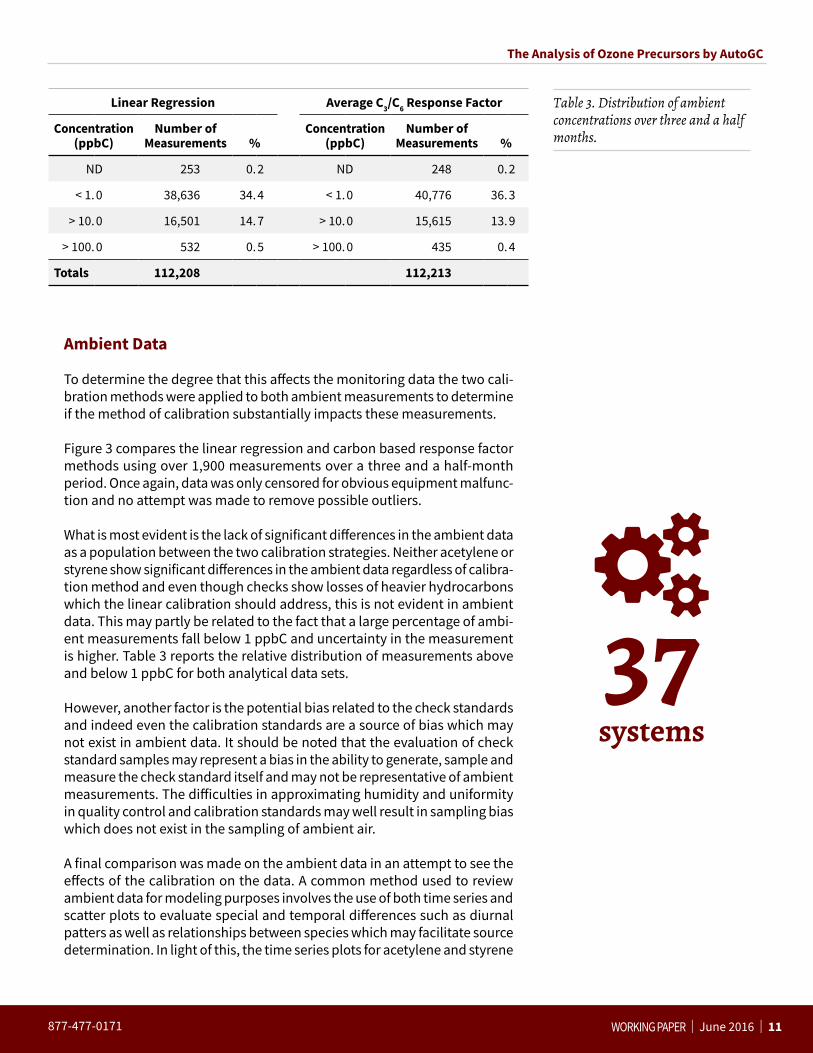
What is most evident is the lack of significant differences in the ambient data as a population between the two calibration strategies. Neither acetylene or styrene show significant differences in the ambient data regardless of calibra-tion method and even though checks show losses of heavier hydrocarbons which the linear calibration should address, this is not evident in ambient data. This may partly be related to the fact that a large percentage of ambi-ent measurements fall below 1 ppbC and uncertainty in the measurement is higher. Table 3 reports the relative distribution of measurements above and below 1 ppbC for both analytical data sets.

However, another factor is the potential bias related to the check standards and indeed even the calibration standards are a source of bias which may not exist in ambient data. It should be noted that the evaluation of check standard samples may represent a bias in the ability to generate, sample and measure the check standard itself and may not be representative of ambient measurements. The difficulties in approximating humidity and uniformity in quality control and calibration standards may well result in sampling bias which does not exist in the sampling of ambient air.

A final comparison was made on the ambient data in an attempt to see the effects of the calibration on the data. A common method used to review ambient data for modeling purposes involves the use of both time series and scatter plots to evaluate special and temporal differences such as diurnal patters as well as relationships between species which may facilitate source determination. In light of this, the time series plots for acetylene and styrene


Concentration (ppbC)

Number of Measurements %

Concentration (ppbC)

Number of Measurements %

ND 253 0.2 ND 248 0.2

< 1.0 38,636 34.4 < 1.0 40,776 36.3

> 10.0 16,501 14.7 > 10.0 15,615 13.9

> 100.0 532 0.5 > 100.0 435 0.4

Totals 112,208 112,213

Table 3. Distribution of ambient concentrations over three and a half months.

37systems


Linear RegressionC

3 /C6 Response Factor

Figure 4. Com

parative time series of concentrations in ppbC for acetylene (top) and styrene (bottom

) calculated with a linear regression calibration (blue) and

a carbon response factor calibration (red).



were compared since these two species demonstrated large discrepancies between calibration methods.

Figure 4 depicts the comparative time series for acetylene (top) and styrene (bottom) respectively. As can be observed the time series for each only var-ies slightly in concentration, thus while the accuracy of the measurement may be different, the precision appears to be good and is not affected by the method of calibration. Since these measurements are in the range of 1–3 ppbC it is difficult to determine which method is truly more accurate.

Likewise, the comparative scatter plots in Figure 5 represents the relationships between acetylene and benzene (top) as well as for styrene and ethylben-zene (bottom). These also show only a slight shift in the response based on the calibration differences. Again, this suggests that the effect seen in the actual artificially derived standards may not be inherent in the ambient air measurements. Overall, the effect of calibration method on these ambient measurements may affect the absolute values but do not appear to change the trends as seen in the ambient population of data.

SUMMARY While there is a definite difference in the results on tested samples manufac-tured either in canisters or by dynamic dilution it is important to remember that the linear regression method of calibration does not remove the lower responses seen across targets. Since the carbon response of the FID has been thoroughly studied and characterized the bias across hydrocarbon species is more likely a function of the thermal desorption process itself and the hardware associated with it. Moreover, this bias may result from the attempt to manufacture suitable test mixtures and may not represent a systematic error in the corresponding ambient measurements.

The implementation of currently available continuous, online AutoGC sys-tems like the ones used here involves more than just a fully automated system. Care must be taken to design a quality management system which is simple and robust to minimize both operator scrutiny and maximize both data quality and data completeness. Systems must be not only well calibrated but designed to make any calibration errors readily observable

Ethylbenzene (ppbC)

Styr

ene

(ppb

C)

Linear Regression

C3/C6 Response FactorLinear Regression

C3/C6 Response Factor

Acet

ylen

e (p

pbC)

Benzene (ppbC)

“Compound specific

linear regression

calibration is

difficult at best...

”

Figure 5. Scatter plots of the rela-tionship between acetylene and benzene (left) and styrene and ethyl-benzene (right).


“...this bias is

reproduced

throughout the

network uniformly

and consistently.

”

to validation team members. Although there are observable differences in the calibration methods used for this analysis, consideration must be given to the complexity of the calibration process as well as the ease with which errors can be observed in such a calibration. Existing NMHC data being used in modeling efforts is based on the carbon-based response strategy and thus consideration must be given to historical data despite biases which may be inherent in this data.

To build a population of data for use in modeling it is important that all data be generated in a similar fashion. While the differences shown here between calibration methods may appear to be of little consequence on the actual data collected, the method of calibration could affect both the overall quality of the data and data recovery. Compound specific linear regression calibration is difficult at best when performed by highly trained laboratory personnel. The use of this type of calibration strategy may result in errors which ultimately would result in faulty measurements and lost data. The ease with which a carbon-based average response factor calibration strategy can be implemented facilitates more frequent calibration without the intense scrutiny required of target specific calibration curves.

Carbon-based calibration has been in use in the PAMS program since its in-ception in 1993. Using the PerkinElmer Ozone Precursor systems, the Texas Commission on Environmental Quality (TCEQ) has been operating AutoGCs for over 20 years and currently has 37 field systems collecting hourly data year round. With a robust network and sound quality control program, the TCEQ is able to see consistent results from many systems. Figure 6 (left) illustrates the combined daily calibration verification standard (CVS) recoveries for 15 targets across 25 PerkinElmer AutoGC systems during a week (nine mea-surements per system). The CVS is a 1 ppmv 15-component certified standard

Figure 6. Distribution of seven (one week of) daily CVS (left) and six (six weeks of) weekly LCS (right) recoveries at 25 sites.



which is diluted to 5 ppbv. The inherent bias is shown for the heavier hydrocarbons and acetylene but this bias is reproduced throughout the network uniformly and consistently. Figure 6 (right) shows recoveries for the same 15 targets across 25 PerkinElmer AutoGC systems of a second source laboratory check standard (LCS) which is run weekly at each site. This standard is blended statically from another 1 ppmv certified standard to 5 ppbv in a canister and run to validate the dynamic dilution system. While the variation in the LCS recoveries is slightly larger, the network consistency is evident and the bias still observable.

By implementing good repeatable instrument configurations as well as monitoring instrument performance via frequent quality control checks, these systems are able to generate large amounts of consistent data across the range of targets.

ACKNOWLEDGEMENTSThe author would like to acknowledge the assistance of Nicola Watson, Markes International and Kelly Beard, Agilent Technologies in the loan of and configuration of the Markes Unity 2 and Agilent Chromatographic system. In addition, Project Managers at the TCEQ; Patti De La Cruz, Cindy Maresh and Melanie Hotchkiss have provided their feedback and continued support of the AutoGC network in Texas. As always Orsat, LLC is eternally grateful for the help and guidance of Lee Marotta and Corey Whipp at PerkinElmer.

REFERENCES 1. United States Environmental Protection Agency. Technical assistance

document for sampling and analysis of ozone precursors. EPA/600-R-98/161; National Exposure Research Laboratory, Human Exposure and Atmospheric Sciences Division: Research Triangle Park, NC, 1998. http://www3.epa.gov/ttnamti1/files/ambient/pams/newtad.pdf (accessed Nov 29, 2015).

2. Cavender, Kevin A. 2015. “Summary of Final Photochemical Assess-ment Monitoring Stations (PAMS) Network Design”. Memorandum OAQPS.

3. Broadway, Graham, and Andrew Tipler. 2009. “Ozone Precursor Analysis Using a Thermal Desorption – GC System.”

4. Markes International. 2013. “Continuous On-Line Monitoring of Hazardous Air Pollutants by TD–GC–FID”. Markes International.

20years


5. Hoerger, C. C.; Claude A.; Plass-Dülmer, C.; Reimann, S.; Eckart, E.; Steinbrecher, R.; Aalto, A.; et al. ACTRIS non-methane hydrocarbon in-tercomparison experiment in Europe to support WMO GAW and EMEP observation networks. Atmos. Meas. Tech. 2015, 8 (7), 2715–2736.

6. Plass-Dülmer, C.; Schmidbauer, N.; Slemr, J.; Slemr, F.; Souza, H. D. Euro-pean hydrocarbon intercomparison experiment AMOHA part 4: Canister sampling of ambient air. J. Geophys. Res. 2006, 111 (D4), D04306.

7. Rappenglück, B.; Apel, E.; Bauerfeind, M.; Bottenheim, J.; Brickell, P.; Čavolka, P.; Cech, J.; et al. The first VOC intercomparison exercise within the Global Atmosphere Watch (GAW). Atmos. Environ. 2006, 40 (39), 7508–7527.

8. United States Environmental Protection Agency. Appendix B to Part 136 – Definition and procedure for the determination of the method detection limit – Revision 1.11. 40 CFR Ch. I (7–1–11 Edition). Washington, DC. http://www.gpo.gov/fdsys/pkg/CFR-2011-title40-vol23/pdf/CFR-2011-title40-vol23-part136-appB.pdf (accessed Nov 29, 2015).

Carol Meyer has been actively involved with PAMS moni-toring since the initial 1993 Coastal Ozone Assessment for Southeastern Texas (COAST) study. Orsat, LLC has provided ambient monitoring services to both state and industry, and currently operates 25 PAMS AutoGC monitor-ing sites in Texas for the TCEQ, UT CEER and AECOM. Using both the PerkinElmer Ozone Precursor system and the Agilent GC System with a Markes Unity 2 thermal desorber, Orsat has developed a fully automated applica-tion for the continuous hourly monitoring of 56 NMHCs.

By implementing

good repeatable

instrument

configurations as

well as monitoring

instrument

performance via

frequent quality

control checks,

these systems are

able to generate

large amounts of

consistent data

across the range of

targets.

“

”

Orsat, LLC1416 Southmore AvePasadena, TX 77502www.orsat.com877-477-0171

Product specifications and descriptions in this document subject to change without notice.

© Orsat, LLC.

Published 05/05/17 5385-EN

Fully Automated, Round-the-Clock, Photochemical Assessment Monitoring Stations (PAMS)Orsat has customized the installation of hardware and software to produce a robust application for the measurement of VOCs in the ambient air known as the AutoGC. Orsat has been involved with continuous unattended ambient air VOC monitoring since its earliest implementation in the State of Texas Coastal Oxidant Assessment for Southeast Texas (COAST) program in 1994. Today, Orsat’s services encompass all aspects of site operation from deployment to operator training and application assistance in topics ranging from Microsoft Windows operation to gas chromatographic theory. Over the past three decades, Orsat has deployed over 40 sites and currently maintains over 35 sites in the state of Texas for both public and private industry. In particular, Orsat has worked closely with the Texas Commission on Environmental Quality (TCEQ) to monitor air quality in the Barnett and Eagle Ford Shale Formations.

the analysis of ozone precursors by autogc - orsat …€¦ · 877-477-0171 working paper | june...

Documents