Western Michigan Ozone Study

Contoured map of measured peak 8-hour ozone concentrations (July 31, 2006)

Final Version

April 24, 2009

Executive Summary

The Energy Policy Act of 2005 requires EPA to conduct “a demonstration project to address the effect of transported ozone and ozone precursors in Southwestern Michigan.” The purpose of this report is to address this requirement by reviewing the ozone problem in Western Michigan and discussing what it will take to meet the federal air quality standards for ozone. On March 12, 2008, the Administrator of EPA signed a final rulemaking establishing a more stringent 8-hour standard for ozone. This report’s technical analyses focus primarily on attainment of the 1997 ozone standard in Western Michigan, however, the results also allow us to draw conclusions relative to the newly promulgated 2008 ozone standard. Ozone levels in Western Michigan exceed both the 1997 and 2008 8-hour ozone federal air quality standards. While ozone levels in this part of the State have declined over the past decade due to federal and state control programs, ambient monitoring data for the past three summers (2006 – 2008) show that the 1997 standard is not being met at only one site (Holland) in Western Michigan, and the 2008 standard is not being met at multiple monitoring sites (Holland, Jenison, Muskegon, and Coloma) in Western Michigan. The key findings of this report are as follows:

• Ozone levels in Western Michigan (both at locations of measured and modeled

nonattainment) are dominated by transport. Western Michigan is impacted by subregional transport of ozone and ozone-forming emissions from major urban areas in the Lake Michigan area (e.g., Chicago, Gary, and Milwaukee) and regional transport of ozone and ozone-forming emissions from other source areas in the eastern U.S. At shoreline locations, the contribution of ozone-forming emissions from sources in Michigan is negligible.

• Analyses of emissions control programs that will be implemented in upwind areas

show that areas in Western Michigan will attain or will be very close to attaining the 1997 ozone standard by June 2009. These projections include emission reductions in upwind areas and no additional local measures in Western Michigan areas.

• Control programs adopted to bring areas into attainment of the 1997 ozone

standard will also make substantial progress toward attainment of the 2008 ozone standard. Projections of future year air quality based on modeling show that all areas in Western Michigan, except Holland, will meet the 2008 ozone standard by 2018. By 2020, all areas in Western Michigan are projected to be in attainment of the 2008 ozone standard.

• The recent court decision to remand the Clean Air Interstate Rule (CAIR) will

have a limited impact on Western Michigan attainment projections. The CAIR is not the sole basis for controls on upwind electric generating units (EGUs).

• The regional approach to air quality planning in the Midwest is an effective

method to address transport and meet air quality goals for the region. Future

i

year analyses of proposed control scenarios indicate that this approach will continue to be effective in lowering ozone concentrations in Western Michigan.

ii

iii

Table of Contents

Section Title Page No. Executive Summary i I Background 1 II Ozone Air Quality in Western Michigan 2 A. Past and Present Ozone Levels 2 B. Understanding Ozone Transport 10 C. Ozone Culpability 15 III Projected Future Year Ozone Levels 18 A. Overview of Modeling Analyses 18 B. Base and Future Year Emissions 18 C. Base Year Modeling 21 D. Future Year Modeling 24 E. Attainment of the 1997 and 2008 Standards 25 V Summary 27 VI References 29 Appendix I Western Michigan Demonstration Project 31 Appendix II Ozone Source Apportionment Modeling Results 32

I. Background On August 8, 2005, the President signed into law the Energy Policy Act of 2005. This national energy plan covers a wide range of areas, including energy efficiency and conservation, alternative and renewable energy sources, and domestic energy production. Title IX, Subtitle I, Section 996 of this Act (see Appendix I) requires EPA to conduct “a demonstration project to address the effect of transported ozone and ozone precursors in Southwestern Michigan.” Ground-level ozone is not emitted directly into the air, but is created by chemical reactions between oxides of nitrogen (NOx) and volatile organic compounds (VOC) - i.e., ozone precursors - in the presence of sunlight. Breathing ozone can trigger a variety of health problems including chest pain, coughing, throat irritation, and congestion. It can worsen bronchitis, emphysema, and asthma. Ground-level ozone also can reduce lung function and inflame the linings of the lungs. Repeated exposure may permanently scar lung tissue. Ground-level ozone also damages vegetation and ecosystems. Under the Clean Air Act, EPA has set protective health-based standards for ozone in the air we breathe. Since 1989, the Lake Michigan Air Directors Consortium (LADCO) has worked with the States of Illinois, Indiana, Michigan, and Wisconsin to address ozone transport in the Lake Michigan region. Through LADCO, the States conducted the Lake Michigan Ozone Study to develop technical tools for SIP planning, addressed regional transport during the Ozone Transport Assessment Group process, and prepared and submitted approvable ozone SIPs for the 1-hour ozone standard. In 1997, EPA adopted an 8-hour ozone standard (0.08 ppm). LADCO and the States have continued to work together on analyses for the 8-hour standard, in preparation for ozone SIPs due in June 2007. On March 27, 2008, EPA’s action promulgating a more stringent 8-hour ozone standard (0.075 ppm) was published in the Federal Register. This final rule was signed by the EPA Administrator on March 12, 2008. The work by LADCO and the States provides the basis for addressing the ozone demonstration project required by the Energy Policy Act of 2005. The report provides a description of the ozone problem in Western Michigan, including the importance of transported ozone into the area and identification of source regions contributing to ozone levels in this part of the State; an examination of the effect of control programs on projected future year ozone levels; and an assessment of the likelihood of attaining the 1997 and 2008 ozone standards in Western Michigan.

1

II. Ozone Air Quality in Western Michigan The State of Michigan operates a network of ground-level ozone monitors throughout the State, which provide data for determining compliance with the federal ozone standard. In Western Michigan, there are 13 monitors in 11 counties (see Figure 1). Many of these monitors have operated since the early 1990’s. A summary of current and historical measured ozone concentrations and a review of the trends in ozone concentrations are provided below.

Figure 1. Ozone Monitoring Sites in Michigan A. Past and Present Ozone Levels The 1997 federal ozone standard is 0.08 parts per million (ppm), averaged over an 8-hour period. The standard is attained if the 3-year average of the 4th-highest daily maximum 8-hour average ozone concentrations (which is referred to as the design value) measured at each monitor within an area is less than 0.08 ppm (or 85 ppb).1 On April 30, 2004 (69 FR 23857), EPA designated 25 counties in the Lower Peninsula as nonattainment for the 8-hour ozone standard (see Figure 2). The designations, which became effective on June 15, 2004, were based on air quality monitoring data for the period 2001 – 2003. Based on more recent data (i.e., for the period 2004 – 2006), EPA redesignated 16 counties in the State to attainment (72 FR 27425, May 16, 2007). Currently, only Allegan

1 For the purpose of this report, ozone concentrations will be expressed in terms of parts per billion (ppb). Although the standard is 0.08 ppm, because of the rounding convention used, a monitor is deemed to be meeting the standard if the 3-year average is less than 0.085 ppm (i.e., 85 ppb). See 40 C.F.R. part 50, App. I, section 2.3

2

County in the Western part of the State and eight counties in the Detroit area are designated as nonattainment of the 8-hour ozone standard. Although designated nonattainment, Allegan County is not currently classified for the 8-hour ozone standard.2

Allegan County

Detroit Nonattainment Counties Lenawee Livingston Macomb Monroe Oakland St. Clair Washtenaw Wayne

Figure 2. Ozone Nonattainment Counties in Michigan On March 27, 2008, EPA promulgated a more stringent 8-hour ozone standard. The 2008 federal ozone standard is 0.075 parts per million (ppm), averaged over an 8-hour period. As with the 1997 8-hour standard, the 2008 standard is attained if the 3-year average of the 4th-highest daily maximum 8-hour average ozone concentrations (which is referred to as the design value) measured at each monitor within an area is less than 0.076 ppm (or 76 ppb). EPA intends to complete nonattainment designations for the more stringent standard by March 2010. The 4th high 8-hour ozone concentrations for 2007 and the design values for the period 2005-2007 are shown in Table 1 and Figure 3. As can be seen, there are only about 20 sites in the

2 Under EPA’s Phase 1 Rule, Allegan County was classified as “basic,” i.e., subject only to the planning provisions of subpart 1 of part D of title I of the Clean Air Act. However, in South Coast Air Quality Management District v. EPA, the Court vacated and remanded the provision of EPA’s Phase 1 Rule that classified certain areas under subpart 1. EPA plans to shortly issue a proposed rule addressing how areas subject to the vacated portion of the rule will be classified for the 1997 8-hour ozone standard.

3

4

Midwest with ozone design values above the 1997 standard, including three sites in Western Michigan: Holland, Muskegon, and Jenison.

Figure 3. Maps of current ozone concentrations in the Midwest – 2007 4th high values (left) and 2005-2007 3-year average 4th high values (right) Even though current (2005-2007) levels at these three sites still exceed the 1997 ozone standard, the levels are much lower than in years past. The change in ozone concentrations over time for the Lake Michigan region is depicted in Figure 4. The maps of design values for several 3-year periods beginning in 1990 show that the spatial extent and magnitude of high ozone concentrations have declined over time in the region. Additional trends information is provided in Figure 5. This figure shows the number of site-days with 8-hour ozone concentrations exceeding 85 ppb3, along with the number of cooling degree days and “hot” days (which provide an indication of ozone conduciveness). As can be seen, there is a general downward trend in this ozone metric. In addition, comparing the top and bottom portions of the figure shows that ozone is strongly influenced by meteorology. That is, the number of site exceedance days is higher during the hotter summers. Interestingly, 2005 had fewer site exceedance days, with respect to the 1997 ozone standard, despite a similar number of hot days and cooling degree days compared to 1995 and 2002, suggesting the importance of recent emission control programs (e.g., reduced power plant NOx emissions beginning in 2004 due to the NOx SIP Call).

3 This “site exceedance” metric provides a measure of the frequency and spatial extent of high ozone days. It is calculated for each year by adding up the number of days with 8-hour concentrations greater than (or equal to) 85 ppb in that year at all monitors in western Michigan.

Table 1. Ozone Concentrations in Western Michigan – 4th High Values and Design Values

4th High Values (ppb) Design Values (ppb)

Site Name County Site ID 2000 2001 2002 2003 2004 2005 2006 2007 '00-'02

'01-'03

'02-'04

'03-'05

'04-'06

'05-'07

3-Year Ave

(2002)

3-Year Ave

(2005) Holland Allegan 260050003 80 92 105 96 79 94 91 94 92 97 93 89 88 93 94.0 90.0 Coloma Berrien 260210014 77 88 98 89 73 90 76 86 87 91 86 84 79 84 88.0 82.3 Cassopolis Cass 260270003 79 88 103 89 77 86 73 83 90 93 89 84 78 80 90.7 80.7 Kalamazoo Kalamazoo 260770008 70 85 90 86 68 81 68 81 81 87 81 78 72 76 83.0 75.3 Jenison Ottawa 261390005 77 86 93 90 69 86 83 88 85 89 84 81 79 85 86.0 81.7 Grand Rapids Kent 260810020 68 83 87 85 68 83 82 84 79 85 80 78 77 83 81.3 79.3 Evans Kent 210810022 73 85 88 93 72 83 81 85 82 88 84 82 78 83 84.7 81.0 Muskegon Muskegon 261210039 78 95 96 94 70 90 90 86 89 95 86 84 83 88 90.0 85.0 Scottville Mason 261050007 81 93 89 88 71 85 76 83 87 90 82 81 77 81 86.3 79.7 Frankfort Benzie 260190003 81 91 86 89 75 86 80 82 86 88 83 83 80 82 85.7 81.7 Seney Schoolcraft 261530001 83 76 74 85 76 85 83 79 77 78 78 82 79.7 79.3 Pashawbestown Leelanau 260890001 79 70 80 73 79 76 74 77 75.6 Manistee Manistee 261010922 83 83 83 ---

Note: values above the 1997 version of the standard are highlighted in red

5

6

Figure 4. Ozone Design Value Maps for 1995-1997, 2000-2002, and 2005-2007

0

20

40

60

80

100

120

140

1981 1986 1991 1996 2001 2006

Site

-Exc

eeda

nce

Day

s

All Sites Kent County and Muskegon County

0

10

20

30

40

50

1981 1986 1991 1996 2001 2006

Hot

Day

s

400.00

600.00

800.00

1000.00

1200.00

1400.00

Coo

ling

Deg

ree

Day

sHot Days Cooling Degree Days

Figure 5. Exceedances of 1997 ozone standard (top) and weather statistics (bottom) for the period 1981 – 2007

Note: ozone statistics are presented both for those sites with a continuous record of data since 1980 (i.e., a few sites in Kent and Muskegon Counties) and for all sites, many of which have been operating only since the early 1990’s Hot Days = number of 90o days measured at Chicago O’Hare Airport Cooling Degree Days = sum of difference between mean daily temperature and 65oF measured at Chicago O’Hare Airport

7

Given the effect of meteorology on ambient ozone levels, year-to-year variations in meteorology can make it difficult to assess trends in ozone air quality. Two approaches were considered to adjust ozone trends for meteorological influences: an air quality-meteorology statistical model developed by EPA (i.e., Cox method), and statistical grouping of meteorological variables performed by LADCO (i.e., Classification and Regression Trees, or CART). Cox Method: This method uses a statistical model to ‘remove’ the annual effect of meteorology on ozone (Cox and Chu, 1993). A regression model was fit to the 1997-2007 data to relate daily peak ozone concentrations to seven daily meteorological variables (daily maximum temperature, midday average relative humidity, morning and afternoon wind speed and wind direction, and morning mixing height), plus seasonal and annual factors. The model is then used to predict 4th high ozone values. By holding the meteorological effects constant, the long-term trend can be examined independent of meteorology. Presumably, this trend reflects the effect of ozone precursor emissions. Figure 6 shows the actual monitored and meteorologically-adjusted 4th high ozone concentrations for the two monitoring sites with the highest ozone concentrations in Western Michigan (Holland and Muskegon). The meteorologically-adjusted data for these sites show a downward trend in the 4th high values. Holland Muskegon

70

75

80

85

90

95

100

105

110

1997 1998 1999 2000 2001 2002 2003 2004 2005 2006 2007

actual 4th high m et-adjusted 4th high

70

75

80

85

90

95

100

105

110

1997 1998 1999 2000 2001 2002 2003 2004 2005 2006 2007

actual 4th high m et-adjus ted 4th high Figure 6. Actual (monitored) and meteorologically-adjusted 4th high 8-hour ozone concentrations for two sites in Western Michigan based on Cox method (1997-2007) CART: Classification and Regression Tree (CART) analysis is another statistical technique which partitions data sets into groups or nodes with similar meteorological conditions (Breiman et al., 1984). The meteorological variables included in the model include surface and aloft wind direction, wind speed, relative humidity, temperature, dewpoint, pressure, mixing height, solar radiation, and cloud cover. Ozone data were examined for the period 1995-2007.

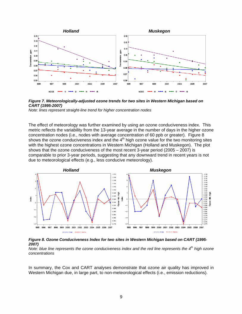
The trends within these groups are then examined. Because the meteorology within each node is similar, the trends over time are ‘adjusted’ for meteorology and should show trends in ozone precursor emissions. Figure 7 shows the higher concentration nodes for the two monitoring sites with the highest ozone concentrations in Western Michigan (Holland and Muskegon). The results for these sites show a downward trend, consistent with the results of the Cox method.

8

Holland Muskegon

Figure 7. Meteorologically-adjusted ozone trends for two sites in Western Michigan based on CART (1995-2007) Note: lines represent straight-line trend for higher concentration nodes The effect of meteorology was further examined by using an ozone conduciveness index. This metric reflects the variability from the 13-year average in the number of days in the higher ozone concentration nodes (i.e., nodes with average concentration of 60 ppb or greater). Figure 8 shows the ozone conduciveness index and the 4th high ozone value for the two monitoring sites with the highest ozone concentrations in Western Michigan (Holland and Muskegon). The plot shows that the ozone conduciveness of the most recent 3-year period (2005 – 2007) is comparable to prior 3-year periods, suggesting that any downward trend in recent years is not due to meteorological effects (e.g., less conducive meteorology). Holland Muskegon

Figure 8. Ozone Conduciveness Index for two sites in Western Michigan based on CART (1995-2007) Note: blue line represents the ozone conduciveness index and the red line represents the 4th high ozone concentrations In summary, the Cox and CART analyses demonstrate that ozone air quality has improved in Western Michigan due, in large part, to non-meteorological effects (i.e., emission reductions).

9

B. Understanding Ozone Transport Previous transport studies: One of the earliest studies of transport in Western Michigan was conducted by the State of Michigan in the late 1980s (Fitzner and Lax, 1988). The purpose of this study was to determine the cause of ozone exceedances in Muskegon. The study considered aircraft measurements, ground-level monitoring, and meteorological analyses. Key study findings include:

• Ozone exceedance days in Muskegon and Grand Rapids are associated with periods of high solar insolation, high temperature, and, especially, south to southwest winds.

• Elevated ozone concentrations in Western Michigan are not limited to Muskegon. High

concentrations extend at least as far south as the Benton Harbor area. (There were insufficient data to determine the northern extent of high concentrations.)

• Emissions from local, Western Michigan counties have a relatively small impact on

ozone exceedances in Western Michigan. This finding is based on aircraft measurements over Lake Michigan showing high precursor concentrations, and upwind/downwind ground-level measurements around Muskegon showing similar levels.

A comprehensive study of ozone transport in the Lake Michigan region (including Western Michigan) was conducted as part of the Lake Michigan Ozone Study (LMOS). The goals of LMOS (and the subsequent Lake Michigan Ozone Control Program) were to collect air quality, meteorological, and emissions data; develop a modeling system for use by the States; and develop, submit, and implement a regional control plan for ozone. A major field program was conducted during the summers of 1990 and 1991 to collect the data. Based on analysis of the LMOS data, a conceptual model of ozone formation and transport in the Lake Michigan region was developed (STI, 1994). According to this model:

• Off-shore flow in the morning transports ozone precursors (from major cities in the southern part of the Lake) into a stable layer over Lake Michigan.

• Over the Lake, ozone production is enhanced by strong atmospheric stability (which

limits dispersion of pollutants), strong solar insolation (due to lack of convective cloud cover), and the absence of any surface removal mechanisms.

• Synoptic winds transport the polluted air mass to downwind locations; to eastern

Wisconsin under southerly flow and to Western Michigan under southwesterly flow4.

• As ozone-laden air flows onshore, air with high concentrations located at low altitudes is mixed down to surface first, causing high ozone concentrations at shoreline monitors.

During the 1991 LMOS field program, exceedances of the 1-hour ozone standard were measured at locations all along the western shore of Michigan from Benton Harbor to Sleeping Bear Dunes National Lakeshore, and even in the Garden Peninsula of the Upper Peninsula. During one multi-day episode in July 1991, every monitoring station along the western coast 4 Cross-lake transport was demonstrated by measurements collected during the LMOS field program, including balloon launches from Chicago, Gary, and Milwaukee on several days with southwesterly winds. The balloons were tracked on a clear path to the northeast and were recovered in Western Michigan.

10

measured a 1-hour exceedance. The large spatial extent of observed ozone exceedances demonstrates that this is not an isolated air quality problem limited to urban areas such as Muskegon, but is actually a Western Michigan regional problem.5 (LADCO, 1992; ENSR, 1991) Based on these studies, it is clear that transport of ozone (and its precursors) is a significant factor and occurs on several spatial scales. Regionally, over a multi-day period, somewhat stagnant summertime conditions can lead to the build-up in ozone and ozone precursor concentrations over a large spatial area. This polluted air mass can be advected long distances, resulting in elevated ozone levels in locations far downwind. An example of such an episode is shown in Figure 9.

Figure 9. Example of Elevated Regional Ozone Concentrations (June 23 – 25, 2005)

Note: plot is based on spatial interpolation of hourly ozone data Locally, emissions from urban areas add to the regional background leading to ozone concentration hot spots downwind. Depending on the synoptic wind patterns (and local land-lake breezes), different downwind areas are affected (see, for example, Figure 10).

Figure 10. Examples of Recent High Ozone Days in the Lake Michigan Area

Note: plot is based on spatial interpolation of hourly ozone data

5 During the 1991 LMOS field program, there were also ozone exceedances in the southern Lake Michigan basin during a multi-day period in mid-June with northeasterly winds. Although sources in Western Michigan likely contributed to these exceedances, a review of historical ozone episodes in the Lake Michigan region found that such conditions were not predominant. About 75% of regional episodes occurred with southerly or southwesterly winds, and only about 10% (or less) with northeasterly winds.

11

Aloft (aircraft) measurements also provide evidence of elevated regional background concentrations and “plumes” from individual urban areas. For one typical summer day with high temperatures and southerly winds (August 20, 2003 – see Figure 11), the incoming background ozone levels were on the order of 80 – 100 ppb and the downwind ozone levels over Lake Michigan were on the order of 100 - 150 ppb.

Figure 11. Aircraft Ozone Measurements over Lake Michigan (left) and Along Upwind Boundary (right) – August 20, 2003

To address the regional transport problem in the eastern U.S., LADCO worked with over 30 states during 1995 – 1997 as part of the Ozone Transport Assessment Group (OTAG). The goal of OTAG was to “...identify and recommend a strategy to reduce transported ozone and its precursors which, in conjunction with other measures, will enable attainment and maintenance of the national ambient ozone standard in the OTAG region.” During its two years of operation, OTAG developed the most comprehensive, up-to-date assessment of ozone transport in the eastern U.S.

Among the major conclusions reached by OTAG are that (OTAG, 1997):

• Regional NOx reductions are effective in producing ozone benefits; the more NOx reduced, the greater the benefit.

• Ozone benefits are greatest in the subregions where emissions reductions are made; the benefits decrease with distance.

• Both elevated (from tall stacks) and low-level NOx reductions are effective.

12

13

• VOC controls are effective in reducing ozone locally and are most advantageous to urban nonattainment areas.

• Air quality data indicate that ozone is pervasive, that ozone is transported, and that ozone aloft is carried over and transported from one day to the next. Ozone transport is evident on several scales: regional (300-500 miles), subregional (100-300 miles), and local (30-150 miles).

• The range of transport is generally longer in the North than in the South.

Based on the OTAG recommendations, in September 1998, EPA called upon 22 States in the eastern half of the U.S. to revise their SIPs to require NOx emissions reductions (i.e., the NOx SIP Call). Current transport patterns: Back trajectories were constructed using the HYSPLIT model for high ozone days (8-hour peak > 80 ppb) during the period 2002-2006 in Western Michigan to characterize general transport patterns. Composite trajectory plots for high ozone days at the two monitoring sites with the highest ozone concentrations in western Michigan (Holland and Muskegon) are provided in Figure 12. The plots point back to areas located to the south-southwest (especially, northeastern Illinois and northwestern Indiana) as being upwind on these high ozone days. The previous and current transport studies demonstrate that:

• Ozone transport is a problem affecting many portions of the eastern U.S. The Lake Michigan region both receives high levels of incoming (transported) ozone and ozone precursors from upwind source areas on many hot summer days, and contributes to the high levels of ozone and ozone precursors affecting downwind receptor areas.

• The presence of a large body of water (i.e., Lake Michigan) influences the formation and

transport of ozone in the region. Depending on large-scale synoptic winds and local-scale lake breezes, different parts of the region experience high ozone concentrations. For example, under southerly flow, high ozone can occur in eastern Wisconsin, and under southwesterly flow, high ozone can occur in Western Michigan.

• Downwind shoreline areas around Lake Michigan are affected by both regional transport

of ozone and subregional transport from major urban areas in the Lake Michigan region. Counties along the western shore of Michigan (from Benton Harbor to Traverse City, and even as far north as the Upper Peninsula) are impacted by high levels of transported ozone.

These last two factors especially distinguish the ozone transport problem in Western Michigan from transport problems in other parts of the country, like the Northeast Corridor.

Figure 12. Contoured trajectory plots for high ozone days at two sites in Western Michigan (2002–2006) Note: darker shading represents higher frequency (e.g., air is most likely to have passed through areas with dark orange shading)

14

C. Ozone Culpability The transport studies show that ozone levels in Western Michigan, especially levels at coastal monitors, are due largely to nearby (e.g., Chicago, Gary, and Milwaukee) and other upwind source regions. Air quality data analyses and modeling studies provide further (quantitative) information on source region and source sector contributions to ambient ozone levels in Western Michigan. A simple comparison of ozone concentrations upwind of Chicago (Braidwood, IL), within Chicago (ten sites in the City), and downwind of Chicago (Holland and Muskegon) was performed for days in 1999 – 2002 with southwesterly winds - i.e., transport towards Western Michigan (Envair, 2005). Figure 13 shows the distribution of daily peak 8-hour ozone concentrations by day-of-week, with a line connecting the mean values. The difference between day-of-week mean values at downwind and upwind sites indicates that the Chicago metropolitan area contributes (on average) about 10-15 ppb to downwind ozone levels.

Figure 13. Mean day-of-week peak 8-hour ozone concentrations at sites upwind, within, and downwind of Chicago, 1999 – 2002 (southwesterly wind days), Cite: Envair, 2005 Further analyses were conducted to assess the effect of changes in precursor emissions in Chicago on downwind ozone levels in Western Michigan (Envair, 2005). For the transport days identified above (i.e., southwesterly flow during the summers of 1999 – 2002), mean NOx concentrations in Chicago are about 50% lower and mean ozone concentrations at the (downwind) Western Michigan sites are about 1.5 – 5.2 ppb (3 – 8 %) lower on Sunday compared to Wednesday. This degree of change in downwind ozone levels suggests a positive, albeit non-linear response to urban area emission reductions. Two modeling studies were conducted to assess source region and source sector contributions. First, as part of the LMOS, LADCO performed sensitivity analyses to identify the maximum impact of three Western Michigan counties (Ottawa, Kent, and Muskegon) and to assess whether emission reductions in these three counties would affect local and domain-wide peak 1-hour ozone concentrations (LADCO, 1994a and 1994b). The results showed: (a) maximum impacts of these counties occurred downwind (outside of the three counties) at locations below the standard, and (b) the contribution of these counties to 1-hour exceedances within the three counties was less than 5 ppb. LADCO’s modeling report concluded that these Western Michigan counties would be able to attain the 1-hour ozone standard, but for the overwhelming

15

transport from nearby upwind nonattainment areas and from areas outside the modeling domain. Second, as part of the SIP development under the 1997 8-hour ozone standard, LADCO performed source apportionment analyses. Specifically, the model was used to estimate the impact of 18 geographic source regions (i.e., state and sub-state areas identified in Figure 14) and 6 source sectors (EGU point, non-EGU point, on-road, off-road, area, and biogenic sources) at ozone monitoring sites in the region.

Muskegon

Holland

Figure 14. Source regions (left) and select monitoring sites (right) for ozone culpability analysis Note: the 18 state and sub-state source regions shown here are represented by different colors Modeling results for 2012 are provided in Figure 15 for the two monitoring sites with the highest ozone concentrations in western Michigan (Holland and Muskegon). (Results for additional monitoring sites in Western Michigan are contained in Appendix II.) For each monitoring site, there are two graphs: one showing sector-level contributions, and one showing source region and sector-level contributions in terms of percentages. (Note, in the sector-level graph, the contribution from NOx emissions are shown in blue, and from VOC emissions in green. For EGUs, several higher emitting facilities were tracked individually and their collective contribution is shown as the red portion of the EGU bar.) The sector-level results show that on-road and off-road NOx emissions generally have the largest contributions at the key monitor locations (> 15% each). EGU and non-EGU NOx emissions are also important contributors (> 10% each). The source region results show that Illinois is the largest contributor (30-40%, with 20-30% alone from the Chicago nonattainment area) at these sites. The only other state with at least a 10% contribution to sites in Western Michigan is Indiana. The contribution from Michigan emissions is very small at shoreline sites in Western Michigan (e.g., less than 3% at Holland and Muskegon)

16

Muskegon

Holland

Figure 15. Model-based ozone source apportionment results for two sites in Western Michigan Note: BC represents the contribution from the boundary conditions

17

III. Projected Future Year Ozone Levels Federal and state regulatory agencies rely on air quality models to support their planning efforts. Models can be used to project future year air quality and conduct “what if” analyses (e.g., assess the effect of emission control programs.) Based on the experience of the LMOS, the Lake Michigan States have been using sophisticated photochemical grid models since the early 1990s to help develop ozone control plans. A. Overview of Modeling Analyses Three sets of modeling analyses provide information about future year ozone levels in Western Michigan:

(1) LADCO Modeling with 2002 Base Year: In mid-2006, LADCO completed modeling using CAMx for a 2002 base year and several future years: 2008, 2009, 2012, and 2018 (LADCO, 2006a). This modeling is referred to as Round 4.

(2) LADCO Modeling with 2005 Base Year: Following completion of LADCO’s Round 4

analyses, LADCO decided to conduct additional modeling (Round 5) using CAMx for a more current base year (2005) and the same four future years (LADCO, 2007a). In light of the U.S. Court of Appeals for the D.C. Circuit’s July 2008 decision to vacate EPA’s Clean Air Interstate Rule (CAIR), which is a major part of the assumed controls in the future year inventories, LADCO conducted an additional analysis to assess the potential impact of the CAIR vacature. On December 23, 2008, the Court reversed its decision and instead decided to remand CAIR to the EPA rather than vacate it in its entirety.

(3) EPA Modeling with 2002 Base Year: As part of their Regulatory Impact Analysis for

the 2008 ozone standard, EPA conducted modeling with CMAQ for a 2002 base year and one future year: 2020 (EPA, 2008a).

All three modeling analyses were performed in accordance with EPA modeling guidelines (EPA, 2007). The results from these analyses are presented below. B. Base and Future Year Emissions For the LADCO modeling, emission inventories were prepared for two base years (2002 and 2005) and four future years (2008, 2009, 2012, and 2018). A summary of the approach for each source sector is summarized below. Further details are provided in two emission inventory reports (LADCO, 2006b and LADCO, 2007b).

On-road Sources: For Round 4, emissions were calculated using vehicle miles traveled (VMT) and MOBILE6 inputs supplied by the LADCO States. Emissions were generated for 36 days (weekday, Saturday, Sunday for each month) at 36 km, and 9 days (weekday, Saturday, Sunday for June – August) at 12 km. For Round 5, emissions were calculated using data (e.g., VMT and vehicle speeds) supplied by state/local planning agencies in the Midwest. Emissions were generated for 6 days (July and January weekday, Saturday, and Sunday). For non-LADCO States, emissions were based on data from other Regional Planning Organizations (RPOs).

18

Off-road Sources: EPA’s NMIM (Round 4) and NMIM2005 (Round 5) models were used to calculate emissions. Additional off-road categories (i.e., commercial marine, aircraft, and railroads) were handled separately. Local data for agricultural equipment, construction equipment, commercial marine, recreational marine, and railroads were prepared by contractors. Area Sources: Data supplied by the LADCO States were used to produce weekday, Saturday, and Sunday emissions for each month. Growth factors were based initially on EGAS (version 5.0), and were subsequently modified (for select priority categories) by examining emissions activity data. For non-LADCO States, emissions were based on data from other RPOs. Point Sources: For non-EGU point sources, data supplied by the LADCO States were used to produce weekday, Saturday, and Sunday emissions for each month. Growth factors were based initially on EGAS (version 5.0), and were subsequently modified (for select priority categories) by examining emissions activity data. For non-LADCO States, emissions were based on data from other RPOs. For EGUs, the annual and summer season emissions were supplied by the states and were temporalized for modeling purposes using profiles based on CEM data. Future year emissions were based on the Integrated Planning Model (IPM) – IPM Version 2.1.9 for Round 4 and IPM Version 3.0 for Round 5. Biogenics: For Round 4, EPA’s BIOME model was used to calculate biogenic emissions. For Round 5, a contractor provided an updated version of the MEGAN biogenics model. MEGAN reflects more regional isoprene emissions compared to BIOME and includes emissions of more precursors of secondary PM2.5 organic carbon mass. Due to a lack of information on future year conditions, the biogenic VOC and NOx emissions were assumed to remain constant between the base year and future years.

The future year emission inventories include the following existing (“on the books”) controls:

On-road Sources – Tier II/Low sulfur fuel – Inspection/Maintenance programs (nonattainment areas) – Reformulated gasoline (nonattainment areas)

Off-road Sources

– Federal control programs incorporated into NONROAD model (e.g., nonroad diesel rule), plus the evaporative Large Spark Ignition and Recreational Vehicle standards

– Heavy-duty diesel (2007) engine standard/Low sulfur fuel – Federal railroad/locomotive standards – Federal commercial marine vessel engine standards

Area Sources

– Aerosol coatings (new rule) – Architectural and industrial maintenance (AIM) coatings (amendments) – Household and institutional consumer products (amendments) – Portable fuel containers (Mobile Source Air Toxics rule)

EGU Point Sources

– Title IV (Phases I and II) – NOx SIP Call

19

– Clean Air Interstate Rule6

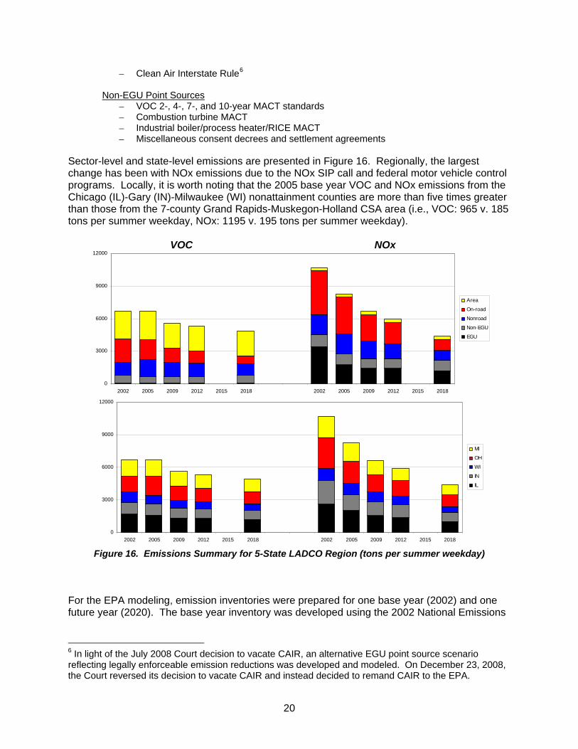
Non-EGU Point Sources – VOC 2-, 4-, 7-, and 10-year MACT standards – Combustion turbine MACT – Industrial boiler/process heater/RICE MACT – Miscellaneous consent decrees and settlement agreements

Sector-level and state-level emissions are presented in Figure 16. Regionally, the largest change has been with NOx emissions due to the NOx SIP call and federal motor vehicle control programs. Locally, it is worth noting that the 2005 base year VOC and NOx emissions from the Chicago (IL)-Gary (IN)-Milwaukee (WI) nonattainment counties are more than five times greater than those from the 7-county Grand Rapids-Muskegon-Holland CSA area (i.e., VOC: 965 v. 185 tons per summer weekday, NOx: 1195 v. 195 tons per summer weekday). VOC NOx

0

3000

6000

9000

12000

2002 2005 2009 2012 2015 2018 2002 2005 2009 2012 2015 2018

Area

On-road

Nonroad

Non-EGU

EGU

0

3000

6000

9000

12000

2002 2005 2009 2012 2015 2018 2002 2005 2009 2012 2015 2018

MI

OH

WI

IN

IL

Figure 16. Emissions Summary for 5-State LADCO Region (tons per summer weekday)

For the EPA modeling, emission inventories were prepared for one base year (2002) and one future year (2020). The base year inventory was developed using the 2002 National Emissions

6 In light of the July 2008 Court decision to vacate CAIR, an alternative EGU point source scenario reflecting legally enforceable emission reductions was developed and modeled. On December 23, 2008, the Court reversed its decision to vacate CAIR and instead decided to remand CAIR to the EPA.

20

Inventory (Version 3). The future year inventory was projected from the base year inventory using activity growth factors and a similar set of “on the books” controls to that listed above. Further details are provided in EPA’s technical modeling report (EPA, 2008b).

21

22

C. Base Year Modeling The first step in the modeling process is to evaluate model performance by comparing modeled and monitored concentrations. An evaluation was conducted using data for 2002 and 2005 with a focus on the magnitude, temporal pattern, and spatial pattern of ozone concentrations. The results presented below are representative of the overall results and demonstrate that the modeling data are in good agreement with the monitoring data. Figure 17 provides a comparison of modeled and monitored hourly ozone concentrations for the two monitoring sites with the highest ozone concentrations in Western Michigan (Holland and Muskegon) for the period mid-June through mid-August 2002.

Figure 17. Hourly modeled and monitored ozone for Muskegon (top) and Holland (bottom) for summer 2002 Note: model results are shown for grid cell with monitor and array of grid cells surrounding monitor Figures 18 and 19 provide spatial maps of modeled and monitored ozone concentrations in the Midwest for two high ozone episodes: one in June 2002 and one in June 2005.. Model performance statistics (bias and error) were also calculated. The results for western Michigan are well within the range of acceptable values identified by EPA: (a) mean bias is generally less than +10% (recommended value is +5-15%), and (b) mean gross error is generally less than 15% (recommended value is 30-35%). EPA’s modeling guidelines recommend that states undertake a “variety of performance tests and weigh them qualitatively to assess model performance.” (EPA, 2007) To this end, Figure 17 shows that the model reproduces the day-to-day variation in ozone concentrations and Figures 18 and 19 show that the model reproduces the spatial pattern of ozone concentrations. Together, the figures and performance statistics show that the magnitude of the modeled concentrations is close to that of the monitored concentrations. Consequently, it can be concluded that the model is a reliable tool for planning purposes.

Figure 18. Modeled (top) v. Monitored (bottom) 8-Hour Ozone Concentrations: June 20 – 25, 2002

23

24

Figure 19. Modeled (top) v. Monitored (bottom) 8-Hour Ozone Concentrations: June 23– 28 2005

D. Future Year Modeling Following a demonstration of acceptable model performance, the next step in the modeling process is to apply the model to project future year air quality concentrations. The results of LADCO’s and EPA’s future year modeling of existing controls are shown in Table 2 (LADCO, 2006a, 2007a; and EPA, 2008a).7

Table 2. Ozone Modeling Results

LADCO Round 4 Results for 2008, 2009, 2012, 2018, and EPA Results for 2020

Site Name County Site ID Base Year* 2008 2009 2012 2018 2020

Holland Allegan 260050003 94.0 84.9 83.5 81.0 76.4 73

Coloma Berrien 260210014 88.0 80.4 79.2 77.4 73.4 70

Cassopolis Cass 260270003 90.7 81.7 80.4 78.1 73.5 68

Kalamazoo Kalamazoo 260770008 83.0 73.9 72.5 70.1 65.4 62

Jenison Ottawa 261390005 86.0 78.7 77.6 75.5 71.7 66

Grand apids Kent 260810020 81.3 73.7 72.7 70.7 66.7 65

Evans Kent 210810022 84.7 76.2 75.0 72.6 68.2 65

Muskegon Muskegon 261210039 90.0 82.7 81.5 79.4 75.5 69

Scottville Mason 261050007 86.3 79.0 77.8 75.5 71.7 65

Frankfort Benzie 260190003 85.7 78.6 77.4 75.2 71.5 66

Seney Schoolcraft 261530001 79.7 72.9 71.1 69.5 65.5 62

* = based on average of three 3-year periods centered on 2002

LADCO Round 5 Results for 2008, 2009, 2012, 2018 and EPA Results for 2020

Site Name County Site ID Base Year* 2008 2009 2012 2018 2020

Holland Allegan 260050003 90.0 85.6 85.3 82.9 76.1 73

Coloma Berrien 260210014 82.3 78.5 78.3 76.2 70.1 70

Cassopolis Cass 260270003 80.7 76.3 75.5 73.1 66.6 68

Kalamazoo Kalamazoo 260770008 75.3 71.0 70.2 67.9 61.7 62

Jenison Ottawa 261390005 81.7 77.6 76.8 74.6 68.4 66

Grand Rapids Kent 260810020 79.3 75.1 74.4 72.1 65.8 65

Evans Kent 210810022 81.0 76.9 76.0 73.6 66.9 65

Muskegon Muskegon 261210039 85.0 80.8 80.5 78.3 71.9 69

Scottville Mason 261050007 79.7 76.0 75.3 73.2 67.6 65

Frankfort Benzie 260190003 81.7 77.9 76.7 74.5 68.4 66

Seney Schoolcraft 261530001 79.3 75.6 75.1 73.0 67.0 62

* = based on average of three 3-year periods centered on 2005

7 In light of the July 2008 Court decision to vacate CAIR, a special model run was conducted by LADCO using the Round 5 inputs with an alternative EGU point source scenario reflecting legally enforceable emission reductions. The results were very similar to those for Round 5, with only marginally higher predicted ozone concentrations (i.e., all sites in Western Michigan were in attainment of the 1997 ozone standard in 2009, except Holland). Again, the Court later changed its decision to vacate CAIR and instead remanded CAIR to EPA.

25

Note: values above the 1997 version of standard are highlighted in red, values above the 2008 version of standard are highlighted in red and blue E. Attainment of 1997 and 2008 Ozone Standards 1997 Standard: Considering the results of the 2002 base year (Round 4) and 2005 base year (Round 5) modeling in Table 2, all monitoring sites in Western Michigan, except Holland, show attainment of the 1997 ozone standard by 2009. Holland’s design value in 2009 is projected to be near the standard (84.9 - 85.6 ppb, depending on the modeling analysis). These results suggest that Western Michigan will be close to meeting the 1997 ozone standard in 2008 and 2009. EPA believes that regional efforts will continue to support significant progress toward meeting the standard. Important factors in whether the standard is actually met by then are the severity of the meteorology during the 3-year period prior to the attainment date, and achievement of emission reductions from existing controls in upwind areas, especially those with the greatest culpability to high ozone in Western Michigan (i.e., Illinois and Indiana). EPA believes the regional approach to air quality planning in the Midwest is the best way to address transport and meet air quality goals for the region. 2008 Standard: EPA plans to designate nonattainment areas for the 2008 ozone standard by March 2010. The most current quality-assured data available at the time designations are issued will be used to determine whether an area will be designated as nonattainment. If designations are promulgated in early 2010, then EPA would rely on data from 2006-2008 or, if quality-assured in time to be considered, then data from 2007-2009. Attainment dates will be based on the severity of an area’s classification and, for areas designated in 2010, maximum attainment dates would range from 2013 (for an area classified as marginal) to 2030 (for an area classified as extreme). EPA plans to issue regulations to govern implementation of the 2008 ozone standard, but anticipate that ozone SIPs demonstrating attainment will be due three years following designation. Based on 2005-2007 and preliminary 2006-2008 monitoring data, the following areas in Western Michigan are violating the 2008 ozone standard (see Table 3): Holland (Allegan County), Benton Harbor (Berrien County), Cass County, Grand Rapids (Kent and Ottawa Counties), Manistee County, Muskegon (Muskegon County), Benzie County, and, possibly, Kalamazoo-Battle Creek (Van Buren, Kalamazoo, and Calhoun Counties)8, Leelanau County, Mason County, and Schoolcraft County. This list is subject to change based on the data available at the time of designation.

8 The Kalamazoo-Battle Creek Metropolitan Statistical Area includes three counties (Van Buren, Kalamazoo, and Calhoun). Only Kalamazoo County has an ozone monitor.

26

Table 3. Latest Ozone Concentrations in Western Michigan

4th High Values (ppb) Design Values (ppb) Site Name County Site ID 2004 2005 2006 2007 2008 '04-'06 '05-'07 '06-'08

Holland Allegan 260050003 79 94 91 94 73 88 93 86 Coloma Berrien 260210014 73 90 76 86 73 79 84 78 Cassopolis Cass 260270003 77 86 73 83 72 78 80 76 Kalamazoo Kalamazoo 260770008 68 81 68 81 70 72 76 73

Jenison Ottawa 261390005 69 86 83 88 68 79 85 79 Grand Rapids Kent 260810020 68 83 82 84 66 77 83 77 Evans Kent 210810022 72 83 81 85 69 78 83 78 Manistee Manistee 261010922 83 83 65 77 Muskegon Muskegon 261210039 70 90 90 86 69 83 88 81 Pashawbestown Leelanau 260890001 70 80 73 79 63 74 77 71

Scottville Mason 261050007 71 85 76 83 66 77 81 75

Frankfort Benzie 260190003 75 86 80 82 68 80 82 76 Seney Schoolcraft 261530001 74 85 76 85 62 78 82 74

Note: values above the 2008 version of the standard are highlighted in blue Considering the results of the 2002 base year (Round 4) and 2005 base year (Round 5) modeling in Table 2, all monitoring sites in Western Michigan, except Holland, Cassopolis, Coloma, and Muskegon, would likely attain the 2008 ozone standard by 2012 and all sites, except Holland, would likely attain the standard by 2018. Holland’s design value in 2018 is projected to be near the standard (either 76.1 or 76.4 ppb, depending on modeling analysis). EPA’s modeling shows that all areas in Western Michigan are likely to attain the 2008 standard by 2020. Upwind areas will be developing attainment plans for the 2008 ozone standard which will include additional control measures not taken into account in the current LADCO and EPA modeling. These additional control measures are expected to further reduce ozone levels in Western Michigan and would likely bring some or all of these areas into attainment with the 2008 standard earlier than predicted by the LADCO and EPA modeling.

27

IV. Summary This report, which was prepared pursuant to the requirements of the Energy Policy Act of 2005, provides:

• a description of the ozone problem in Western Michigan, including the importance of transported ozone into the area and identification of source regions contributing to ozone levels in this part of the State;

• an examination of the effect of control programs on projected future year ozone

levels; and

• an assessment of the likelihood of attaining the 1997 and 2008 ozone standards in Western Michigan.

Based on an examination of monitoring data and air quality modeling studies, the following key findings should be noted:

• Current ambient monitoring data show nonattainment with the 1997 ozone standard for the following areas in Western Michigan: Holland and, possibly, Muskegon and Jenison. Modeling analyses indicate that other locations in Western Michigan may also have air quality levels above the 1997 federal ozone standard.

• Current (2006-2008) ambient monitoring data show nonattainment with the 2008

ozone standard for the following areas in Western Michigan: Holland (Allegan County), Benton Harbor (Berrien County), Grand Rapids (Kent and Ottawa Counties), Manistee County, Muskegon (Muskegon County), and Benzie County.

• Ozone levels in Western Michigan (both at locations of measured and modeled

nonattainment) are dominated by transport.

• Trends in historical air quality data show that ozone levels in Western Michigan have improved over time due to emission reductions from existing control programs.

• Projections of future year air quality estimates show that Muskegon and Jenison

will likely meet the 1997 standard by 2009. Holland will be close to meeting the 1997 standard with emission reductions from existing control programs.

• Control programs adopted to bring areas into attainment of the 1997 ozone

standard will significantly contribute to attainment of the 2008 ozone standard. Projections of future year air quality based on modeling show that all areas in Western Michigan except Holland will meet the 2008 ozone standard by 2018. By 2020, all areas in Western Michigan are projected to be in attainment of the 2008 ozone standard.

• The regional approach to air quality planning in the Midwest is an effective

method to address transport and meet air quality goals for the region. Future

28

year analyses of proposed control scenarios indicate that this approach will continue to be effective in lowering ozone concentrations in Western Michigan.

29

V. References Breiman, L., J. Friedman, R. Olshen, and C. Stone, Classification and Regression Trees, Chapman & Hall (1984) Cox, W.M, and S.-H. Chu, Meteorologically Adjusted Ozone Trends in Urban Areas: A Probabililistic Approach, Atmospheric Environment 27B(4):425-434 (1993). Fitzner, C. and J. Lax, 1988, “Mesoscale Transport of Ozone: Determination at a Lake Michigan Shoreline Community”, in “The Scientific and Technical Issues Facing Post 1987 Ozone Control Strategies”, Air & Waste Management Association, 1988 ENSR, 1991, “Summary of LMOS 1991 Field Measurements, 1991”, ENSR Consulting & Engineering Envair, 2005, “Weekday/Weekend Differences in Ambient Concentrations of Primary and Secondary Air Pollutants in Atlanta, Baltimore, Chicago, Dallas-Fort Worth, Denver, Houston, New York, Phoenix, Washington, and Surrounding Areas”, NREL Project ES04-1, July 30, 2005 EPA, 2007, “Guidance on the Use of Models and Other Analyses for Demonstrating Attainment of Air Quality Goals for Ozone, PM2.5, and Regional Haze”, April 2007, EPA-454/B-07-002. EPA, 2008a, “Final Ozone NAAQS Regulatory Impact Analysis”, March 2008. EPA, 2008b, “Air Quality Modeling Platform for the Ozone National Ambient Air Quality Standard, Final Rule, Regulatory Impact Analysis.” Kenski, D., 2007, “CART Analysis for Ozone Trends and Meteorological Similarity”, May 10, 2007 LADCO, 1992, “The Lake Michigan Ozone Study – Summer 1991 Field Measurements”, Lake Michigan Air Directors Consortium, E2M Journal, Summer 1992 LADCO, 1994a, “Impact of Moderate Nonattainment Areas”, Lake Michigan Air Directors Consortium, March 17, 1994 LADCO, 1994b, “Technical Support Document, Modeling Demonstration to Support an Attainment Date Extension for the Western Michigan Moderate Ozone Nonattainment Areas”, Lake Michigan Air Directors Consortium, November 8, 1994 LADCO, 2006a, “Base K/Round 4 Modeling: Summary”, Lake Michigan Air Directors Consortium, August 31, 2006 LADCO, 2006b, “Base K/Round 4 Strategy Modeling: Emissions”, Lake Michigan Air Directors Consortium, May 16, 2006 LADCO, 2007a, “Base M/Round 5 Modeling: Summary”, Lake Michigan Air Directors Consortium, October 2007

30

LADCO, 2007b, “Base M/Round 5 Strategy Modeling: Emissions”, Lake Michigan Air Directors Consortium, August 2007 OTAG, 1997, “Ozone Transport Assessment Group, Executive Report”, 1997 STI, 1994, “Air Quality Data Analysis for the 1991 Lake Michigan Ozone Study”, Final Report, Sonoma Technology, Inc., September 1994

31

Appendix I SEC. 996. WESTERN MICHIGAN DEMONSTRATION PROJECT The Administrator of the Environmental Protection Agency, in consultation with the State of Michigan and affected local officials, shall conduct a demonstration project to address the effect of transported ozone and ozone precursors in Southwestern Michigan. The demonstration program shall address projected non-attainment areas in Southwestern Michigan that include counties with design values for ozone of less than .095 based on years 2000 to 2002 or the most current 3-year period of air quality data. The Administrator shall assess any difficulties such areas may experience in meeting the 8-hour national ambient air quality standard for ozone due to the effect of transported ozone or ozone precursors into the areas. The Administrator shall work with State and local officials to determine the extent of ozone and ozone precursor transport, to assess alternatives to achieve compliance with the 8-hour standard apart from local controls, and to determine the timeframe in which such compliance could take place. The Administrator shall complete this demonstration project no later than 2 years after the date of enactment of this section and shall not impose any requirement or sanction under the Clean Air Act (42 U.S.C. 7401 et seq.) that might otherwise apply during the pendency of the demonstration project. (excerpt from the Energy Policy Act of 2005)

32

33

Appendix II

Ozone Source Apportionment Modeling Results

Figure II-1a. Model-based ozone source apportionment results for sites in Western Michigan – Evans (top), Grand Rapids (middle), and Jenison (bottom)

34

Figure II-1b. Model-based ozone source apportionment results for sites in Western Michigan - Kalamazoo (top), Cass County (middle), and Coloma (bottom)

35

36

Figure II-1c. Model-based ozone source apportionment results for sites in Western Michigan – Seney (top), Frankfort (middle), and Scottville (bottom)