the analysis of fatal accidents in indian coal...

THE ANALYSIS OF FATAL ACCIDENTS IN INDIANCOAL MINES

A. Mandal

D. Sengupta1

Indian Statistical Institute, 203 B.T. Road, Calcutta - 700035.

Abstract

This paper describes the analysis of fatal accidents of Indian coal mines from April 1989 to March1998. It is found that Indian mines have considerably higher accident and fatality rates compared tothose in USA and South Africa, respectively. While open cast mines are generally known to be safer thanunderground mines, the Indian open cast mines are shown to be at least as hazardous to the workers as theIndian underground mines. Analysis of the accident rates is made via a few regression models involvingthe effects of working shifts, the various companies, the types of mine, manshift and production. Theaccident-prone combinations of mine type and company are identified for follow-up action. The break-upof the accidents by cause is also studied.

Key words: Linear models, Generalised Linear Models, Analysis of Variance, Poisson Pro-cess, Accident rate, Fatality rate.

AMS Subject Classification Number: Primary 6207, Secondary 62P99, 62N05.

1Address for correspondence : Applied Statistics Unit, Indian Statistical Institute, 203 B.T.Road, Cal-cutta, West Bengal, India. PIN 700035. email:< [email protected] >

1

1 Introduction

Coal is an important mineral in India. Besides being the main source of fuel in powerplants, it is also used in household cooking throughout the country. The coal industryemploys over 600,000 miners and other workers. Safety in the Indian coal mines is thereforea very important issue. However, there has been no significant statistical analysis of thesafety records of Indian coal mines.

The fatal accident rates in India and US during the period 1989-97 are shown in Table 1.The data for the US mines are taken from the Work Time Quarterly Reports of Mine Safetyand Health Administration, the US Department of Labour ( http://www.msha.gov/STATS/PART50/WQ/1978/ wq78c105.htm), while the data for the Indian mines are taken fromthe Fatal Accident Register and Annual Performance Report of Coal India Limited (CIL).

Table 1. Fatal accident rates in US and India, 1989-97 2

Accidents per Accidents permillion tons of million manhours

production per year per yearYear India USA India USA1989 0.722 0.077 0.112 0.051990 0.638 0.071 0.105 0.041991 0.587 0.068 0.103 0.041992 0.644 0.060 0.118 0.041993 0.541 0.055 0.103 0.041994 0.484 0.049 0.099 0.041995 0.468 0.050 0.103 0.041996 0.383 0.040 0.089 0.041997 0.380 0.030 0.091 0.03

A cursory glance at the above table reveals that the yearly accident rates (standardizedby production) in India is consistently higher than the corresponding rate in the USA bya factor of about ten. Differences in the levels of productivity is not the only explanationfor this discrepancy, since the yearly accident rates (standardized by manhours) is alsoconsistently higher in India than in USA by a factor of two to three. Thus, there seems tobe a wide scope for improvement in the safety practices in India.

This paper presents an analysis of the fatal coal mine accidents in India, and attemptsto identify a few problem areas for safety.

All matters relating to the mining, processing and marketing of coal in India is overseenby CIL, which is an umbrella organisation. There are eight subsidiaries or regional compa-nies working under CIL. These are Eastern Coalfields Limited (ECL), Bharat Coking CoalLimited (BCCL), Central Coalfields Limited (CCL), Northern Coalfields Limited (NCL),Western Coalfields Limited (WCL), South-Eastern Coalfields Limited (SECL), MahanadiCoalfields Limited (MCL) and North-Eastern Collieries (NEC). The companies have differ-ent number of active mines, amount of production and the number of manshifts in a givenyear. The companies also have largely exclusive managements, although some amount of

2The U.S. production data, originally given in short tons, have been converted to tons. The Indian yearlyfigures are for the period starting from the month of April of the reported year till the month of March ofthe following year.

2

coordination is achieved through a common board of directors. Some of the companies havemostly underground mines, while the majority of mines in other companies are open cast.NCL has no underground mine.

There are two broad categories of mines in India: Open Cast and Underground. Theaccident records classify the location of accident as underground, open cast and surface.While the first two categories represent accidents occurring inside the two types of mines,respectively, the third category represents mining-related accidents occurring above thesurface in the vicinity of either type of mine. Accordingly, for the present analysis, we usea variable named ‘type’ which can have three possible values: underground (ug), opencast(oc) and surface (su).

In the cases of accidents occurring in underground or open cast mines the produc-tion/manpower in that category for the relevant period has been used for standardization.In the case of accidents occurring on the surface, scaling has been done using the totalproduction/manpower for that company in the relevant period.

In the following sections, attempts have been made to answer several questions of gen-eral interest. In Section 2, we examine whether the inter-accident times are exponentiallydistributed, so that a Poisson process model of the incidence of accidents may be used. InSection 3 we check whether the widely believed hypothesis that open cast mines are saferthan underground mines (see Murty and Panda, 1988, pp. 127–132, and Melinkov andChesnokov, 1969, pp. 21–22) is valid in the Indian context. We compare the safety recordsof the eight companies in Section 4. We examine the effects of the working shift and monthof the year on the incidence of accidents in Sections 5 and 6, respectively. Thus, in Sections3–6, we consider the effects of four categorical variables, taking one variable at a time. InSection 7 we look for a single regression model that incorporates all these variables, startingwith a model similar to that used by Lawrence and Marsh (1984). In this section we lookfor the partial effects of each factor mentioned above in the presence of the other factors. InSection 8 we fit an exponential regression model for the inter-accident times. In Section 9we identify the major causes of the accidents. We provide some concluding remarks inSection 10.

Data on the date and time of an accident, the corresponding working shift, cause ofaccident and the age of the victims were obtained from the Fatal Accident Register of CIL.Data for the period April, 1989 to March, 1998 have been used for the current analysis.The Annual Performance Reports of CIL were the source for data on companywise yearlyproduction and the total number of manshifts. The production and manshift figures ofMCL for the year 1989-90 to 1991-92 were not available.

2 Distribution of inter-accident times

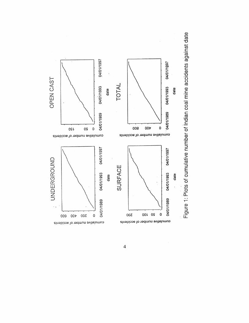
Cox and Lewis (1966) had used a plot of the cumulative number of accidents against thenumber of days, while analyzing the coal mine disasters (accidents involving at least 10deaths) in Britain. A similar plot for all the fatal accidents in Indian coal mines during theperiod April 1989 to March 1998 is given in Figure 1. The figure shows, in addition to thetotal accident counts, the accident counts for underground and open cast mines as well assurface accident counts. All the plots are somewhat linear, with a hint of concavity in thecase of the total number of accidents (bottom right plot). This is in contrast with Figure1.1 of Cox and Lewis (1966), which is clearly concave, exhibiting the effect of safer modesof production and better safety practices in recent times. The lack of concavity in the plots

3

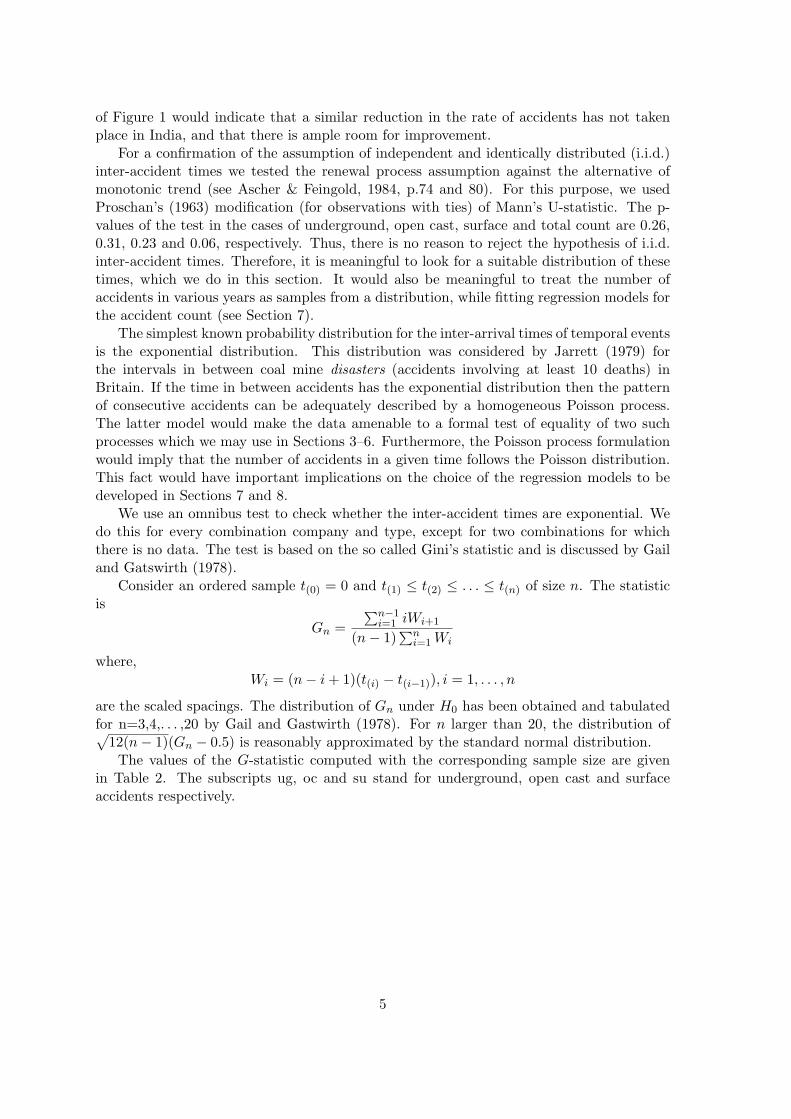
of Figure 1 would indicate that a similar reduction in the rate of accidents has not takenplace in India, and that there is ample room for improvement.

For a confirmation of the assumption of independent and identically distributed (i.i.d.)inter-accident times we tested the renewal process assumption against the alternative ofmonotonic trend (see Ascher & Feingold, 1984, p.74 and 80). For this purpose, we usedProschan’s (1963) modification (for observations with ties) of Mann’s U-statistic. The p-values of the test in the cases of underground, open cast, surface and total count are 0.26,0.31, 0.23 and 0.06, respectively. Thus, there is no reason to reject the hypothesis of i.i.d.inter-accident times. Therefore, it is meaningful to look for a suitable distribution of thesetimes, which we do in this section. It would also be meaningful to treat the number ofaccidents in various years as samples from a distribution, while fitting regression models forthe accident count (see Section 7).

The simplest known probability distribution for the inter-arrival times of temporal eventsis the exponential distribution. This distribution was considered by Jarrett (1979) forthe intervals in between coal mine disasters (accidents involving at least 10 deaths) inBritain. If the time in between accidents has the exponential distribution then the patternof consecutive accidents can be adequately described by a homogeneous Poisson process.The latter model would make the data amenable to a formal test of equality of two suchprocesses which we may use in Sections 3–6. Furthermore, the Poisson process formulationwould imply that the number of accidents in a given time follows the Poisson distribution.This fact would have important implications on the choice of the regression models to bedeveloped in Sections 7 and 8.

We use an omnibus test to check whether the inter-accident times are exponential. Wedo this for every combination company and type, except for two combinations for whichthere is no data. The test is based on the so called Gini’s statistic and is discussed by Gailand Gatswirth (1978).

Consider an ordered sample t(0) = 0 and t(1) ≤ t(2) ≤ . . . ≤ t(n) of size n. The statisticis

Gn =∑n−1

i=1 iWi+1

(n− 1)∑n

i=1 Wi

where,Wi = (n− i + 1)(t(i) − t(i−1)), i = 1, . . . , n

are the scaled spacings. The distribution of Gn under H0 has been obtained and tabulatedfor n=3,4,. . . ,20 by Gail and Gastwirth (1978). For n larger than 20, the distribution of√

12(n− 1)(Gn − 0.5) is reasonably approximated by the standard normal distribution.The values of the G-statistic computed with the corresponding sample size are given

in Table 2. The subscripts ug, oc and su stand for underground, open cast and surfaceaccidents respectively.

5

Table 2: Values of the Gini statistic for various type-company combinations

n Gug n Goc n Gsu

ECL 162 0.500 21 0.446 37 0.493BCCL 203 0.521 40 0.560 48 0.484CCL 53 0.518 55 0.499 48 0.518NCL NA - 25 0.527 8 0.516WCL 92 0.521 24 0.534 14 0.540SECL 101 0.482 33 0.439 30 0.573MCL 10 0.637 12 0.590 16 0.444NEC 10 0.651 3 0.396 0 -

The null hypothesis is accepted at 95% level in all the cases, i.e., all the inter-accidenttimes follow the exponential distribution.

The insignificance of the statistics may have been due to the lack of power of the (non-parametric) test and the shortage of data in some cases. Hence, we had also carried outparametric tests of exponentiality within the Gamma and Weibull families of distributions,by checking whether the shape parameter in each case is equal to 1. The results confirm thefindings reported above. We refer the reader to Mandal and Sengupta (1999) for a detailedreport of these tests as well as the Q-Q plots for checking exponentiality in each case.

3 Are open cast mines safer?

Each of the companies has two technologically different types of mines, namely undergroundand open cast. Only the NCL does not have any underground mine. All companies havesome accidents occurring outside the mine, which are classified under “surface accidents”.

It is generally believed that open cast mines are safer than underground mines (seeMelinkov and Chesnokov, 1969, pp. 21–22). In the case of USA, the MSHA data suggestthat during the period 1989 to 1997, the number of accidents in underground mines per mil-lion tons of production per year was on the average 3.8 times higher than the correspondingrate in open cast mines. This discrepancy is partially due to the greater productivity ofopen cast mines. It is also due in part to the lesser risk to the miners in open cast mines.This is illustrated by the fact that the number of accidents per million manhours per yearin the underground mines is 2.1 times higher than the corresponding rate in the open castmines, after averaging over the yearly figures for the period 1989 to 1997 in the USA.

In the case of Indian mines, the yearly number of accidents per million tons of productionfor underground, open cast and surface happen to be 1.236, 0.144 and 0.102, respectively.The rate is 0.526 when all the types are combined. (Here, pooled data for all the years fromApril 1989 to March 1998 and all the eight companies have been used.) This suggests that fora fixed amount of production, accidents are about 8.5 times more frequent in undergroundmines than in open cast mines. The factor is much larger than the corresponding factor inthe US. This may be because of drastically less productivity of underground mines comparedto the open cast mines in India and/or greater safety of workers in open cast mines comparedto the underground mines in India.

If the latter of these two confounded factors is significant, its effect should be reflected inthe rate of accidents in India, scaled by manshift. The yearly number of accidents per millionmanshifts for underground, open cast and surface are 0.687, 0.579 and 0.160, respectively.The rate is 0.822 when all the types are combined. (Once again, pooled data for all the

6

years from April 1989 to March 1998 and all the eight companies have been used.) It isclear that the number of accidents per million manshifts in open cast and undergroundmines are comparable. Therefore, for a given worker, working in an open cast mine is notless hazardous. This is quite remarkable, in view of the perceived safety of open cast minesin general and the US records in particular.

As a clarification, we note that all the ‘surface’ accidents in India occur in the vicinityof the mine. Unlike in the US, there is no remote facility which caters to over-the-surfaceprocessing or maintenance of equipment for a collection of mines. Thus, in an undergroundmine in India, the ‘underground’ accident count excludes the ‘surface’ accidents whichcorrespond to the same manshift figures. The ‘open cast’ accident counts similarly excludethe surface accidents associated with the common manshift figures. This is why we comparedthe ratio of accident rates in underground and open cast mines in India and USA, ratherthan comparing the rates themselves.

4 Are all companies equally safe?

4.1 Summary statistics

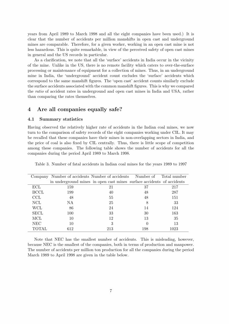
Having observed the relatively higher rate of accidents in the Indian coal mines, we nowturn to the comparison of safety records of the eight companies working under CIL. It maybe recalled that these companies have their mines in non-overlapping sectors in India, andthe price of coal is also fixed by CIL centrally. Thus, there is little scope of competitionamong these companies. The following table shows the number of accidents for all thecompanies during the period April 1989 to March 1998.

Table 3. Number of fatal accidents in Indian coal mines for the years 1989 to 1997

Company Number of accidents Number of accidents Number of Total numberin underground mines in open cast mines surface accidents of accidents

ECLBCCLCCLNCLWCLSECLMCLNECTOTAL

15919948

NA86

1001010

612

214055252433123

213

3748488

1430130

198

21728715133

1241633513

1023

Note that NEC has the smallest number of accidents. This is misleading, however,because NEC is the smallest of the companies, both in terms of production and manpower.The number of accidents per million ton production for all the companies during the periodMarch 1989 to April 1998 are given in the table below.

7

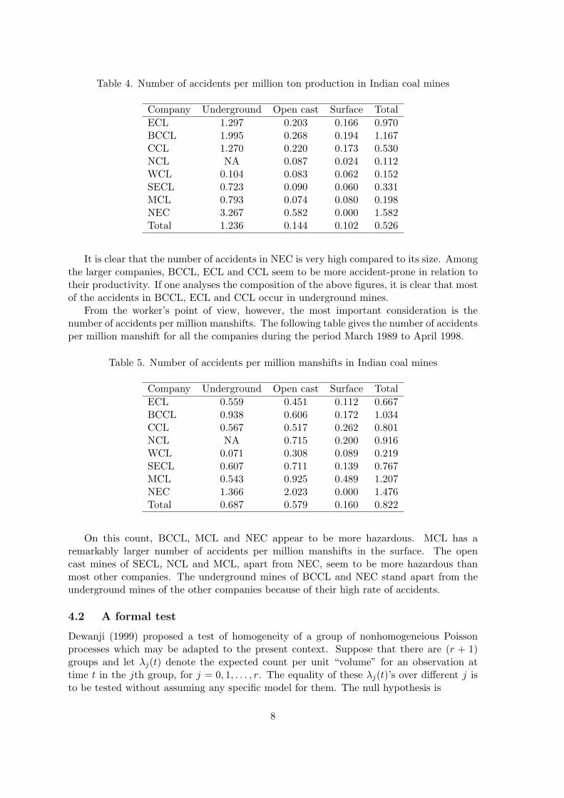
Table 4. Number of accidents per million ton production in Indian coal mines

Company Underground Open cast Surface TotalECL 1.297 0.203 0.166 0.970BCCL 1.995 0.268 0.194 1.167CCL 1.270 0.220 0.173 0.530NCL NA 0.087 0.024 0.112WCL 0.104 0.083 0.062 0.152SECL 0.723 0.090 0.060 0.331MCL 0.793 0.074 0.080 0.198NEC 3.267 0.582 0.000 1.582Total 1.236 0.144 0.102 0.526

It is clear that the number of accidents in NEC is very high compared to its size. Amongthe larger companies, BCCL, ECL and CCL seem to be more accident-prone in relation totheir productivity. If one analyses the composition of the above figures, it is clear that mostof the accidents in BCCL, ECL and CCL occur in underground mines.

From the worker’s point of view, however, the most important consideration is thenumber of accidents per million manshifts. The following table gives the number of accidentsper million manshift for all the companies during the period March 1989 to April 1998.

Table 5. Number of accidents per million manshifts in Indian coal mines

Company Underground Open cast Surface TotalECL 0.559 0.451 0.112 0.667BCCL 0.938 0.606 0.172 1.034CCL 0.567 0.517 0.262 0.801NCL NA 0.715 0.200 0.916WCL 0.071 0.308 0.089 0.219SECL 0.607 0.711 0.139 0.767MCL 0.543 0.925 0.489 1.207NEC 1.366 2.023 0.000 1.476Total 0.687 0.579 0.160 0.822

On this count, BCCL, MCL and NEC appear to be more hazardous. MCL has aremarkably larger number of accidents per million manshifts in the surface. The opencast mines of SECL, NCL and MCL, apart from NEC, seem to be more hazardous thanmost other companies. The underground mines of BCCL and NEC stand apart from theunderground mines of the other companies because of their high rate of accidents.

4.2 A formal test

Dewanji (1999) proposed a test of homogeneity of a group of nonhomogeneious Poissonprocesses which may be adapted to the present context. Suppose that there are (r + 1)groups and let λj(t) denote the expected count per unit “volume” for an observation attime t in the jth group, for j = 0, 1, . . . , r. The equality of these λj(t)’s over different j isto be tested without assuming any specific model for them. The null hypothesis is

8

H0 : λ0(t) = λ1(t) = . . . = λr(t) = λ(t), say, for all t.Let t1 < t2 . . . < tk be the different observation times. Also, let nij denote the count

for a volume aij observed at time ti and in the jth group, for i = 1, 2, . . . , k and j =0, 1, . . . r. Write λij = λj(ti). Then, nij has the Poisson distribution with mean aijλij ,for i = 1, . . . , k and j = 1, . . . , r.

Note that, under H0,

λi0 = λi1 = . . . = λir = λi, say, for i = 1, . . . , k.

The conditional expectations and variances are

E(nij |ni.) = ni.aij

ai.= eij

V ar(nij |ni.) = ni.aij

ai.(1− aij

ai.) = Vjj(i), say,

and Cov(nij , nij′ |ni.) = −ni.aijaij′

a2i.

, for j 6= j′

= Vjj′(i), say.

where ai. =∑r

j=0 aij and ni. =∑r

j=0 nij

Consider the vector dTi = (di0, di1, . . . , dir), where dij = nij−eij is the difference between

observed and expected counts in the (i, j)th cell. Note that, given ni., the random vector di

has zero expectation and variance-covariance matrix given by Vi, the (j, j′)th entry of whichis Vjj′(i). Let

d =∑k

1 di and V =∑k

1 Vi.

The test of homogeneity proposed by Dewanji (1999) is based on an asymptotic χ2(r)

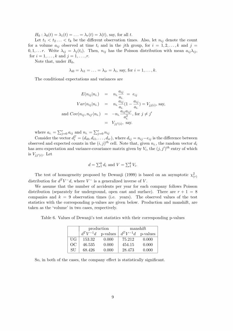
distribution for dT V −d, where V − is a generalized inverse of V .We assume that the number of accidents per year for each company follows Poisson

distribution (separately for underground, open cast and surface). There are r + 1 = 8companies and k = 9 observation times (i.e. years). The observed values of the teststatistics with the corresponding p-values are given below. Production and manshift, aretaken as the ‘volume’ in two cases, respectively.

Table 6. Values of Dewanji’s test statistics with their corresponding p-values

production manshiftdT V −1d p-values dT V −1d p-values

UG 153.32 0.000 75.212 0.000OC 46.535 0.000 454.15 0.000SU 68.426 0.000 28.473 0.000

So, in both of the cases, the company effect is statistically significant.

9

5 Are all the shifts equally risky ?

5.1 Summary statistics

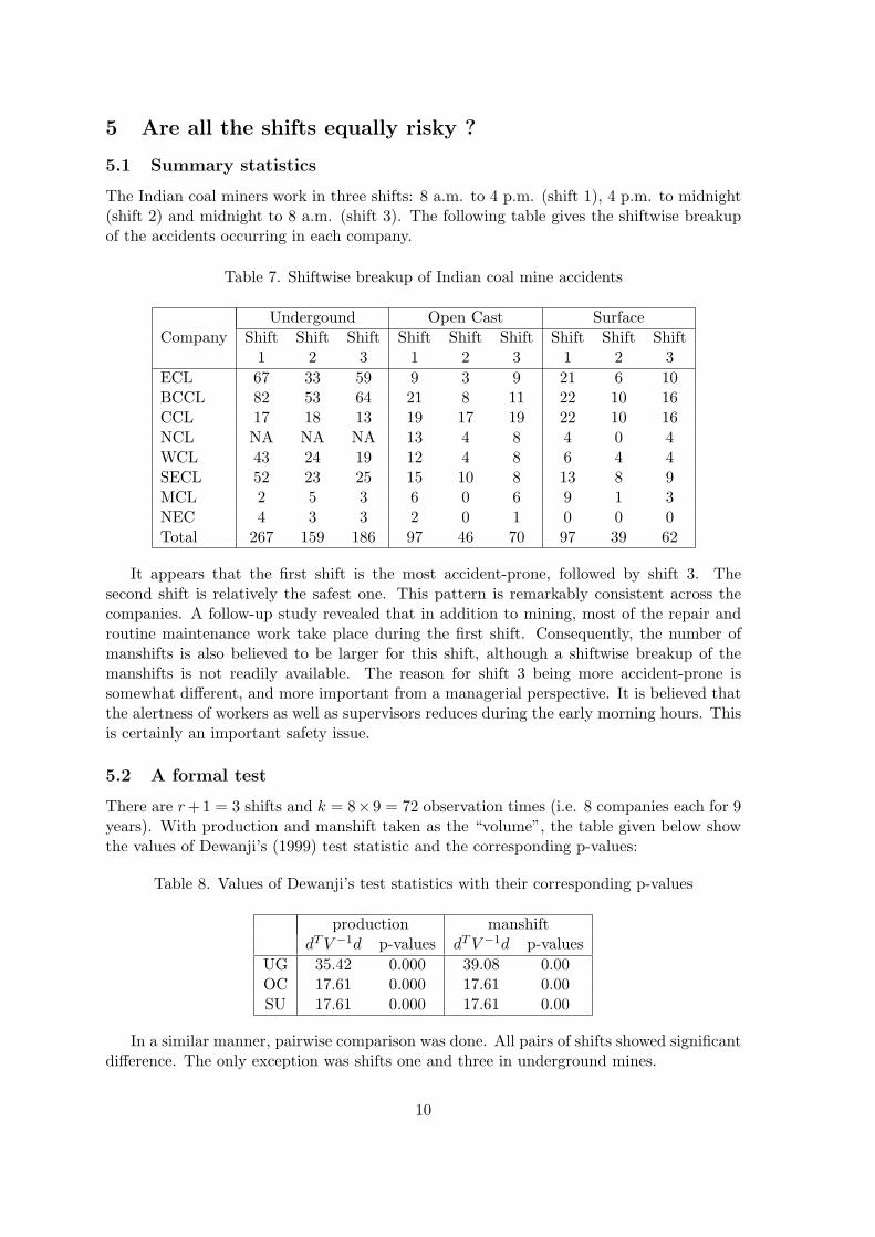
The Indian coal miners work in three shifts: 8 a.m. to 4 p.m. (shift 1), 4 p.m. to midnight(shift 2) and midnight to 8 a.m. (shift 3). The following table gives the shiftwise breakupof the accidents occurring in each company.

Table 7. Shiftwise breakup of Indian coal mine accidents

Undergound Open Cast SurfaceCompany Shift Shift Shift Shift Shift Shift Shift Shift Shift

1 2 3 1 2 3 1 2 3ECL 67 33 59 9 3 9 21 6 10BCCL 82 53 64 21 8 11 22 10 16CCL 17 18 13 19 17 19 22 10 16NCL NA NA NA 13 4 8 4 0 4WCL 43 24 19 12 4 8 6 4 4SECL 52 23 25 15 10 8 13 8 9MCL 2 5 3 6 0 6 9 1 3NEC 4 3 3 2 0 1 0 0 0Total 267 159 186 97 46 70 97 39 62

It appears that the first shift is the most accident-prone, followed by shift 3. Thesecond shift is relatively the safest one. This pattern is remarkably consistent across thecompanies. A follow-up study revealed that in addition to mining, most of the repair androutine maintenance work take place during the first shift. Consequently, the number ofmanshifts is also believed to be larger for this shift, although a shiftwise breakup of themanshifts is not readily available. The reason for shift 3 being more accident-prone issomewhat different, and more important from a managerial perspective. It is believed thatthe alertness of workers as well as supervisors reduces during the early morning hours. Thisis certainly an important safety issue.

5.2 A formal test

There are r +1 = 3 shifts and k = 8×9 = 72 observation times (i.e. 8 companies each for 9years). With production and manshift taken as the “volume”, the table given below showthe values of Dewanji’s (1999) test statistic and the corresponding p-values:

Table 8. Values of Dewanji’s test statistics with their corresponding p-values

production manshiftdT V −1d p-values dT V −1d p-values

UG 35.42 0.000 39.08 0.00OC 17.61 0.000 17.61 0.00SU 17.61 0.000 17.61 0.00

In a similar manner, pairwise comparison was done. All pairs of shifts showed significantdifference. The only exception was shifts one and three in underground mines.

10

6 Is there any seasonal effect ?

We used the following formulation for checking the effect of the month of the year on theaccident count. We compiled all the accidents occurring in the ith month of the jth year,(i = 1, 2, . . . 12, j = 1, 2, . . . , 10). [Note that the accident count for the year April’98–March’99 could not be used earlier because the manshift figures for this year was not avail-able.] We conducted one-way analysis of variance for each type of accident (underground,open cast and surface), with 10 observations per cell, to test for the month effect. Thep-values of the usual F-statistic, under the assumption of normality, turned out to be 0.674,0.483 and 0.758 for underground, open cast and surface, respectively. Thus, month effectcan be safely ruled out.

It may be noted that there was no perceptible month effect in the case of the disasterdata for British coal mines, reported by Jarrett (1979).

7 Regression models for accident count

The results of the foregoing sections suggest that the company, type of mines (underground,open cast, surface) and shift (shift 1, shift 2, shift 3) have considerable effect on the accidentcount, when scaled by production or manshift. On the other hand, the effect of the monthmay be ignored. In this section, we try and build a model which incorporates the first threefactors, along with production and manshift. Since the manshift data was available onlytill March 1998, the data on other variables for the period April 1998 to March 1999 havebeen ignored in this section.

7.1 Linear Regression

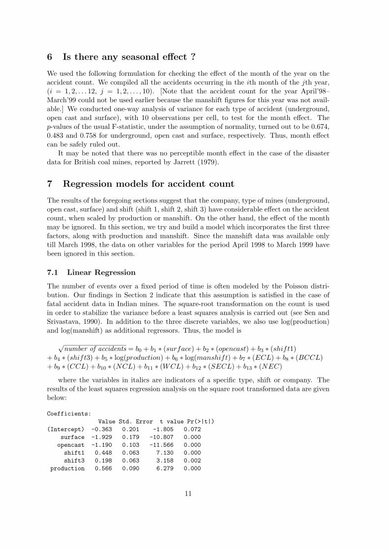
The number of events over a fixed period of time is often modeled by the Poisson distri-bution. Our findings in Section 2 indicate that this assumption is satisfied in the case offatal accident data in Indian mines. The square-root transformation on the count is usedin order to stabilize the variance before a least squares analysis is carried out (see Sen andSrivastava, 1990). In addition to the three discrete variables, we also use log(production)and log(manshift) as additional regressors. Thus, the model is

√number of accidents = b0 + b1 ∗ (surface) + b2 ∗ (opencast) + b3 ∗ (shift1)

+ b4 ∗ (shift3) + b5 ∗ log(production) + b6 ∗ log(manshift) + b7 ∗ (ECL) + b8 ∗ (BCCL)+ b9 ∗ (CCL) + b10 ∗ (NCL) + b11 ∗ (WCL) + b12 ∗ (SECL) + b13 ∗ (NEC)

where the variables in italics are indicators of a specific type, shift or company. Theresults of the least squares regression analysis on the square root transformed data are givenbelow:

Coefficients:Value Std. Error t value Pr(>|t|)

(Intercept) -0.363 0.201 -1.805 0.072surface -1.929 0.179 -10.807 0.000opencast -1.190 0.103 -11.566 0.000

shift1 0.448 0.063 7.130 0.000shift3 0.198 0.063 3.158 0.002

production 0.566 0.090 6.279 0.000

11

manshift -0.024 0.045 -0.524 0.601ecl 0.845 0.114 7.436 0.000bccl 1.114 0.112 9.944 0.000ccl 0.779 0.111 6.990 0.000ncl 0.088 0.136 0.646 0.519wcl 0.514 0.120 4.272 0.000secl 0.371 0.120 3.079 0.002nec 1.373 0.271 5.057 0.000

Residual standard error: 0.625 on 580 degrees of freedomMultiple R-Squared: 0.519F-statistic: 48.08 on 13 and 580 degrees of freedom, the p-value is 0

It is observed from the above results that all the regression coefficients except for thoseof the intercept term, log(manshift) and NCL, are statistically significant at any reasonablelevel. Thus, all the companies except for NCL have a significantly higher accident countcompared to MCL, after taking into account the linear effect of the other variables. Ahistogram of the residuals of the above regression showed an expected bell-shaped pattern.This plot is not given here. The plot confirmed the effectiveness of the variance stabilizingtransformation. [A similar plot for the untransformed count data was found to be skewedheavily to the right.]

The above analysis indicates that accidents are more common inside underground mines,when the effect of production and manshift are taken into account in the manner describedabove. A similar analysis reveals that accidents in open cast mines are also significantlymore frequent than surface accidents.

The preliminary analysis of Section 5 had suggested that shift 1 is the most unsafe, whileshift 2 is the safest. The above analysis confirms that shifts 1 and 3 are significantly moreunsafe than shift 2. A follow-up analysis reveals that shift 1 is significantly more unsafethan shift 3.

The company effects as found from the above analysis generally follow the trend of thepreliminary analyses of Section 4. NEC and BCCL stand out as the companies which areby far the most unsafe.

7.2 Generalized Linear Model (Poisson family)

The variance stabilizing transformation on the accident count data made it amenable toleast squares regression. However, since there is sufficient evidence that the accident counthas Poisson distribution, an appropriate regression model would be the generalized linearmodel for Poisson family. The model is

E(log(number of accidents)) = b0 + b1 ∗ (surface) + b2 ∗ (opencast) + b3 ∗ (shift1)+ b4 ∗ (shift3) + b5 ∗ log(production) + b6 ∗ log(manshift) + b7 ∗ (ECL) + b8 ∗ (BCCL)+ b9 ∗ (CCL) + b10 ∗ (NCL) + b11 ∗ (WCL) + b12 ∗ (SECL) + b13 ∗ (NEC)

Note that, while analyzing explosion-related accidents in the coal mines of USA, Lawrenceand Marsh (1984) had used a linear regression model very similar to the above one (with adifferent set of discrete predictors). The results of the analysis of the GLM are given below.

12

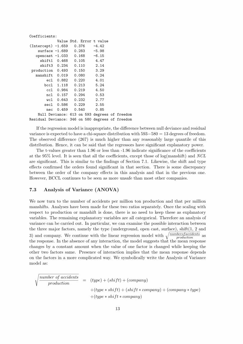
Coefficients:Value Std. Error t value

(Intercept) -1.659 0.376 -4.42surface -1.689 0.283 -5.98

opencast -1.033 0.168 -6.15shift1 0.468 0.105 4.47shift3 0.234 0.110 2.14

production 0.493 0.150 3.29manshift 0.019 0.080 0.24

ecl 0.882 0.220 4.01bccl 1.118 0.213 5.24ccl 0.984 0.219 4.50ncl 0.157 0.294 0.53wcl 0.643 0.232 2.77secl 0.586 0.229 2.55nec 0.459 0.540 0.85

Null Deviance: 613 on 593 degrees of freedomResidual Deviance: 346 on 580 degrees of freedom

If the regression model is inappropriate, the difference between null deviance and residualvariance is expected to have a chi-square distribution with 593−580 = 13 degrees of freedom.The observed difference (267) is much higher than any reasonably large quantile of thisdistribution. Hence, it can be said that the regressors have significant explanatory power.

The t-values greater than 1.96 or less than -1.96 indicate significance of the coefficientsat the 95% level. It is seen that all the coefficients, except those of log(manshift) and NCLare significant. This is similar to the findings of Section 7.1. Likewise, the shift and typeeffects confirmed the orders found significant in that section. There is some discrepancybetween the order of the company effects in this analysis and that in the previous one.However, BCCL continues to be seen as more unsafe than most other companies.

7.3 Analysis of Variance (ANOVA)

We now turn to the number of accidents per million ton production and that per millionmanshifts. Analyses have been made for these two ratios separately. Once the scaling withrespect to production or manshift is done, there is no need to keep these as explanatoryvariables. The remaining explanatory variables are all categorical. Therefore an analysis ofvariance can be carried out. In particular, we can examine the possible interaction betweenthe three major factors, namely the type (underground, open cast, surface), shift(1, 2 and3) and company. We continue with the linear regression model with

√numberofaccidents

production asthe response. In the absence of any interaction, the model suggests that the mean responsechanges by a constant amount when the value of one factor is changed while keeping theother two factors same. Presence of interaction implies that the mean response dependson the factors in a more complicated way. We symbolically write the Analysis of Variancemodel as:

√number of accidents

production= (type) + (shift) + (company)

+(type ∗ shift) + (shift ∗ company) + (company ∗ type)+(type ∗ shift ∗ company)

13

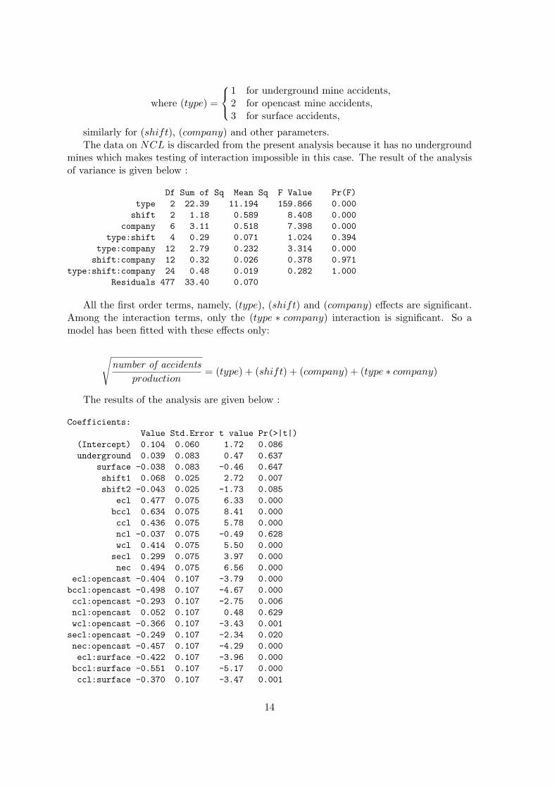
where (type) =

1 for underground mine accidents,2 for opencast mine accidents,3 for surface accidents,

similarly for (shift), (company) and other parameters.The data on NCL is discarded from the present analysis because it has no underground

mines which makes testing of interaction impossible in this case. The result of the analysisof variance is given below :

Df Sum of Sq Mean Sq F Value Pr(F)type 2 22.39 11.194 159.866 0.000shift 2 1.18 0.589 8.408 0.000

company 6 3.11 0.518 7.398 0.000type:shift 4 0.29 0.071 1.024 0.394

type:company 12 2.79 0.232 3.314 0.000shift:company 12 0.32 0.026 0.378 0.971

type:shift:company 24 0.48 0.019 0.282 1.000Residuals 477 33.40 0.070

All the first order terms, namely, (type), (shift) and (company) effects are significant.Among the interaction terms, only the (type ∗ company) interaction is significant. So amodel has been fitted with these effects only:


production= (type) + (shift) + (company) + (type ∗ company)

The results of the analysis are given below :

Coefficients:Value Std.Error t value Pr(>|t|)

(Intercept) 0.104 0.060 1.72 0.086underground 0.039 0.083 0.47 0.637

surface -0.038 0.083 -0.46 0.647shift1 0.068 0.025 2.72 0.007shift2 -0.043 0.025 -1.73 0.085

ecl 0.477 0.075 6.33 0.000bccl 0.634 0.075 8.41 0.000ccl 0.436 0.075 5.78 0.000ncl -0.037 0.075 -0.49 0.628wcl 0.414 0.075 5.50 0.000

secl 0.299 0.075 3.97 0.000nec 0.494 0.075 6.56 0.000

ecl:opencast -0.404 0.107 -3.79 0.000bccl:opencast -0.498 0.107 -4.67 0.000ccl:opencast -0.293 0.107 -2.75 0.006ncl:opencast 0.052 0.107 0.48 0.629wcl:opencast -0.366 0.107 -3.43 0.001

secl:opencast -0.249 0.107 -2.34 0.020nec:opencast -0.457 0.107 -4.29 0.000ecl:surface -0.422 0.107 -3.96 0.000bccl:surface -0.551 0.107 -5.17 0.000ccl:surface -0.370 0.107 -3.47 0.001

14

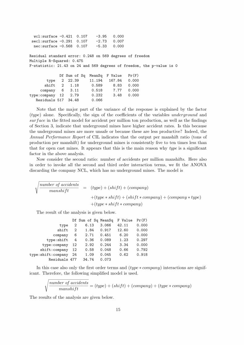
wcl:surface -0.421 0.107 -3.95 0.000secl:surface -0.291 0.107 -2.73 0.007nec:surface -0.568 0.107 -5.33 0.000


Df Sum of Sq MeanSq F Value Pr(F)type 2 22.39 11.194 167.84 0.000shift 2 1.18 0.589 8.83 0.000

company 6 3.11 0.518 7.77 0.000type:company 12 2.79 0.232 3.48 0.000

Residuals 517 34.48 0.066

Note that the major part of the variance of the response is explained by the factor(type) alone. Specifically, the sign of the coefficients of the variables underground andsurface in the fitted model for accident per million ton production, as well as the findingsof Section 3, indicate that underground mines have higher accident rates. Is this becausethe underground mines are more unsafe or because these are less productive? Indeed, theAnnual Performance Report of CIL indicates that the output per manshift ratio (tons ofproduction per manshift) for underground mines is consistently five to ten times less thanthat for open cast mines. It appears that this is the main reason why type is a significantfactor in the above analysis.

Now consider the second ratio: number of accidents per million manshifts. Here alsoin order to invoke all the second and third order interaction terms, we fit the ANOVAdiscarding the company NCL, which has no underground mines. The model is


manshift= (type) + (shift) + (company)

+(type ∗ shift) + (shift ∗ company) + (company ∗ type)+(type ∗ shift ∗ company)

The result of the analysis is given below.


company 6 2.71 0.451 6.20 0.000type:shift 4 0.36 0.089 1.23 0.297

type:company 12 2.92 0.244 3.34 0.000shift:company 12 0.58 0.048 0.66 0.792

type:shift:company 24 1.09 0.045 0.62 0.918Residuals 477 34.74 0.073

In this case also only the first order terms and (type ∗ company) interactions are signif-icant. Therefore, the following simplified model is used.√

number of accidentsmanshift

= (type) + (shift) + (company) + (type ∗ company)

The results of the analysis are given below.

15

Coefficients:Value Std.Error t value Pr(>|t|)

(Intercept) 0.211 0.065 3.24 0.001underground -0.094 0.089 -1.05 0.293

surface -0.088 0.089 -0.99 0.324shift1 0.089 0.027 3.31 0.001shift2 -0.065 0.027 -2.39 0.017

ecl 0.287 0.082 3.52 0.001bccl 0.413 0.082 5.06 0.000ccl 0.265 0.082 3.25 0.001ncl 0.019 0.082 0.23 0.816wcl 0.342 0.082 4.19 0.000

secl 0.287 0.082 3.52 0.001nec 0.282 0.082 3.46 0.001

ecl:opencast -0.253 0.115 -2.20 0.029bccl:opencast -0.261 0.115 -2.27 0.024ccl:opencast -0.096 0.115 -0.83 0.406ncl:opencast 0.125 0.115 1.08 0.281wcl:opencast -0.494 0.115 -4.28 0.000

secl:opencast -0.051 0.115 -0.44 0.661nec:opencast -0.219 0.115 -1.90 0.058ecl:surface -0.269 0.115 -2.33 0.020bccl:surface -0.336 0.115 -2.92 0.004ccl:surface -0.154 0.115 -1.34 0.183wcl:surface -0.362 0.115 -3.14 0.002secl:surface -0.239 0.115 -2.08 0.038nec:surface -0.413 0.115 -3.58 0.000



company 6 2.71 0.45 6.35 0.00type:company 12 2.92 0.24 3.43 0.00

Residuals 517 36.76 0.07

Although the three main effects and the type∗company interaction effect are statisticallysignificant, the residual sum of squares is much higher than the sum of squares explainedby these factors. This indicates that the accident count per million manshifts is somewhatevenly spread across various combinations of factors.

Although the coefficients of underground and surface are not statistically significant,these are much smaller than the coefficient of opencast in the analysis of number of ac-cidents per million manshifts. (Note that the implied coefficient of opencast is 0.) Thisis a remarkable outcome of the analysis. It means that, when the number of accidents isviewed in relation to the number of manshifts involved, open cast mines are equally unsafe,if not more unsafe, than underground mines. This confirms the findings of Section 3. Themessage is that Indian open cast mines are more productive (as expected), but these arenot safer, although common knowledge (see Melinkov and Chesnokov, 1969, pp. 21–22 andWork Time Quarterly Reports) suggest that these should be safer.

16

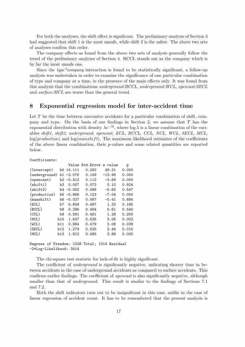
For both the analyses, the shift effect is significant. The preliminary analysis of Section 3had suggested that shift 1 is the most unsafe, while shift 2 is the safest. The above two setsof analyses confirm this order.

The company effects as found from the above two sets of analysis generally follow thetrend of the preliminary analyses of Section 4. BCCL stands out as the company which isby far the most unsafe one.

Since the type*company interaction is found to be statistically significant, a follow-upanalysis was undertaken in order to examine the significance of one particular combinationof type and company at a time, in the presence of the main effects only. It was found fromthis analysis that the combinations underground:BCCL, underground:WCL, opencast:SECLand surface:MCL are worse than the general trend.

8 Exponential regression model for inter-accident time

Let T be the time between successive accidents for a particular combination of shift, com-pany and type. On the basis of our findings in Section 2, we assume that T has theexponential distribution with density λe−λt, where log λ is a linear combination of the vari-ables shift1, shift2, underground, opencast, ECL, BCCL, CCL, NCL, WCL, SECL, MCL,log(production) and log(manshift). The maximum likelihood estimates of the coefficientsof the above linear combination, their p-values and some related quantities are reportedbelow.

Coefficients:Value Std.Error z value p

(Intercept) b0 14.111 0.292 48.31 0.000(underground) b1 -2.076 0.149 -13.98 0.000(opencast) b2 -0.412 0.112 -3.69 0.000(shift1) b3 0.007 0.073 0.10 0.924(shift2) b4 -0.052 0.086 -0.60 0.547(production) b5 -0.866 0.123 -7.04 0.000(manshift) b6 -0.027 0.067 -0.41 0.684(ECL) b7 0.659 0.497 1.33 0.185(BCCL) b8 0.296 0.484 0.61 0.540(CCL) b9 0.591 0.461 1.28 0.200(NCL) b10 1.637 0.535 3.06 0.002(WCL) b11 0.994 0.479 2.08 0.038(SECL) b12 1.279 0.525 2.44 0.015(MCL) b13 1.912 0.495 3.86 0.000

Degrees of Freedom: 1028 Total; 1014 Residual-2*Log-Likelihood: 3414

The chi-square test statistic for lack-of-fit is highly significant.The coefficient of underground is significantly negative, indicating shorter time in be-

tween accidents in the case of underground accidents as compared to surface accidents. Thisconfirms earlier findings. The coefficient of opencast is also significantly negative, althoughsmaller than that of underground. This result is similar to the findings of Sections 7.1and 7.2.

Both the shift indicators turn out to be insignificant in this case, unlike in the case oflinear regression of accident count. It has to be remembered that the present analysis is

17

based on much larger number of cases as compared to the earlier analysis. Specifically,there are 1028 cases in this analysis as opposed to the 594 cases for the analysis of yearlyaccident count data.

The coefficients of the indicators of various companies are generally in line with thefindings of Sections 3 and 7.

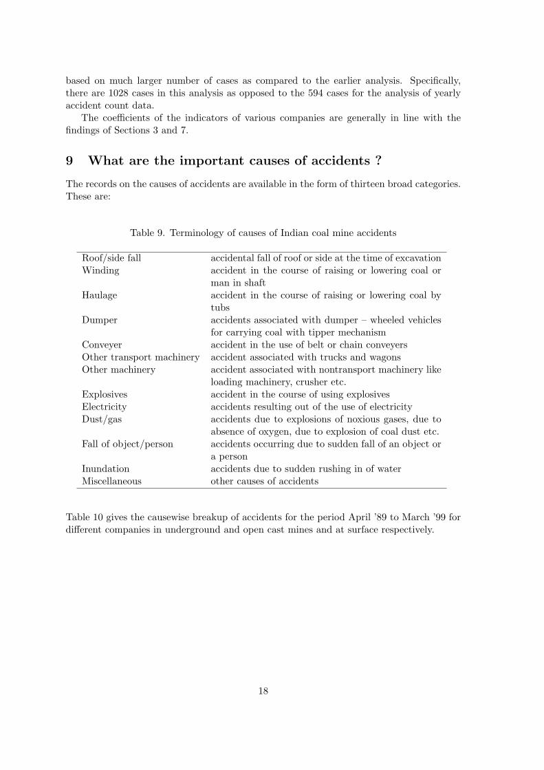
9 What are the important causes of accidents ?

The records on the causes of accidents are available in the form of thirteen broad categories.These are:

Table 9. Terminology of causes of Indian coal mine accidents

Roof/side fall accidental fall of roof or side at the time of excavationWinding accident in the course of raising or lowering coal or

man in shaftHaulage accident in the course of raising or lowering coal by

tubsDumper accidents associated with dumper – wheeled vehicles

for carrying coal with tipper mechanismConveyer accident in the use of belt or chain conveyersOther transport machinery accident associated with trucks and wagonsOther machinery accident associated with nontransport machinery like

loading machinery, crusher etc.Explosives accident in the course of using explosivesElectricity accidents resulting out of the use of electricityDust/gas accidents due to explosions of noxious gases, due to

absence of oxygen, due to explosion of coal dust etc.Fall of object/person accidents occurring due to sudden fall of an object or

a personInundation accidents due to sudden rushing in of waterMiscellaneous other causes of accidents

Table 10 gives the causewise breakup of accidents for the period April ’89 to March ’99 fordifferent companies in underground and open cast mines and at surface respectively.

18

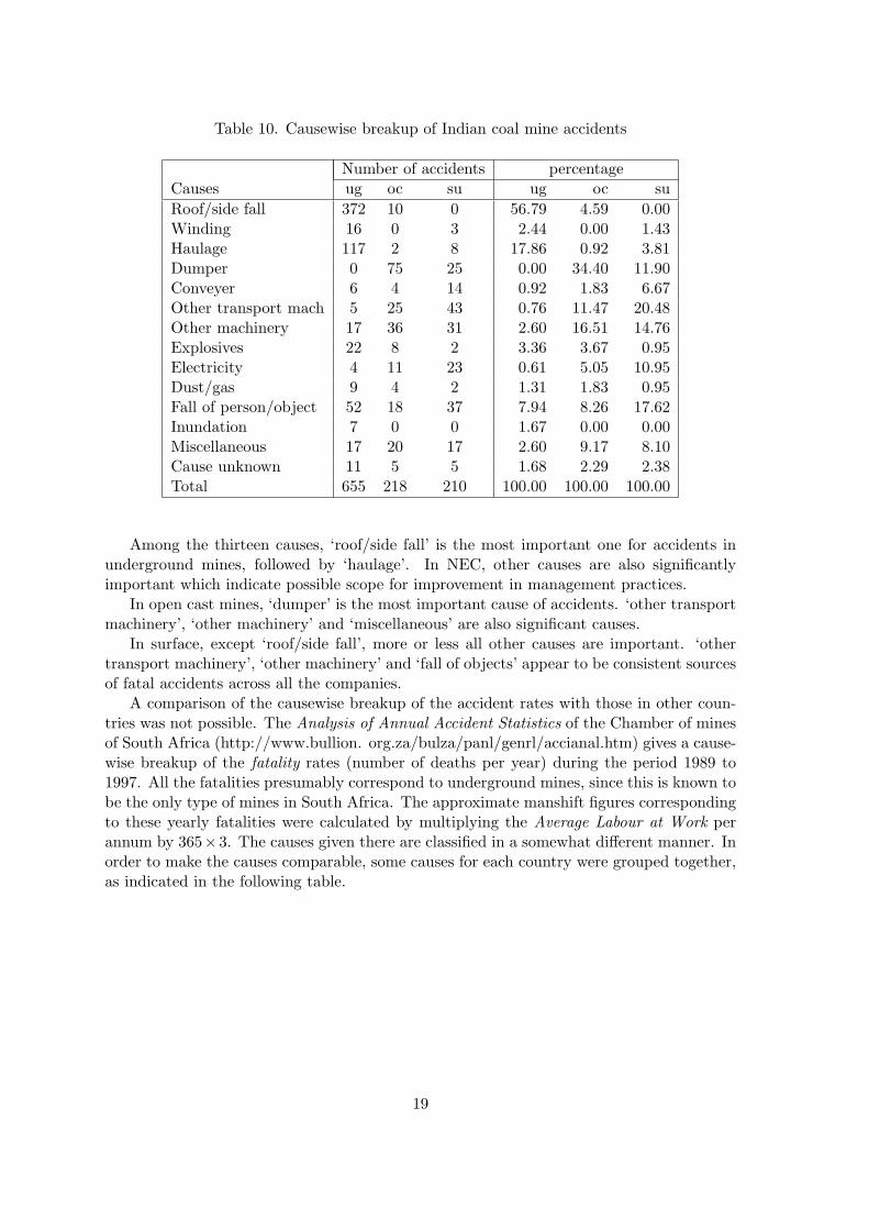
Table 10. Causewise breakup of Indian coal mine accidents

Number of accidents percentageCauses ug oc su ug oc suRoof/side fall 372 10 0 56.79 4.59 0.00Winding 16 0 3 2.44 0.00 1.43Haulage 117 2 8 17.86 0.92 3.81Dumper 0 75 25 0.00 34.40 11.90Conveyer 6 4 14 0.92 1.83 6.67Other transport mach 5 25 43 0.76 11.47 20.48Other machinery 17 36 31 2.60 16.51 14.76Explosives 22 8 2 3.36 3.67 0.95Electricity 4 11 23 0.61 5.05 10.95Dust/gas 9 4 2 1.31 1.83 0.95Fall of person/object 52 18 37 7.94 8.26 17.62Inundation 7 0 0 1.67 0.00 0.00Miscellaneous 17 20 17 2.60 9.17 8.10Cause unknown 11 5 5 1.68 2.29 2.38Total 655 218 210 100.00 100.00 100.00

Among the thirteen causes, ‘roof/side fall’ is the most important one for accidents inunderground mines, followed by ‘haulage’. In NEC, other causes are also significantlyimportant which indicate possible scope for improvement in management practices.

In open cast mines, ‘dumper’ is the most important cause of accidents. ‘other transportmachinery’, ‘other machinery’ and ‘miscellaneous’ are also significant causes.

In surface, except ‘roof/side fall’, more or less all other causes are important. ‘othertransport machinery’, ‘other machinery’ and ‘fall of objects’ appear to be consistent sourcesof fatal accidents across all the companies.

A comparison of the causewise breakup of the accident rates with those in other coun-tries was not possible. The Analysis of Annual Accident Statistics of the Chamber of minesof South Africa (http://www.bullion. org.za/bulza/panl/genrl/accianal.htm) gives a cause-wise breakup of the fatality rates (number of deaths per year) during the period 1989 to1997. All the fatalities presumably correspond to underground mines, since this is known tobe the only type of mines in South Africa. The approximate manshift figures correspondingto these yearly fatalities were calculated by multiplying the Average Labour at Work perannum by 365×3. The causes given there are classified in a somewhat different manner. Inorder to make the causes comparable, some causes for each country were grouped together,as indicated in the following table.

19

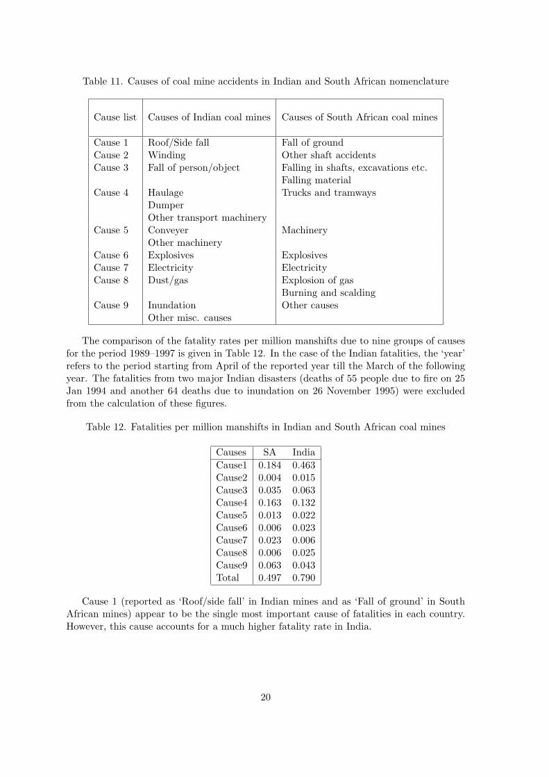
Table 11. Causes of coal mine accidents in Indian and South African nomenclature

Cause list Causes of Indian coal mines Causes of South African coal mines

Cause 1 Roof/Side fall Fall of groundCause 2 Winding Other shaft accidentsCause 3 Fall of person/object Falling in shafts, excavations etc.

Falling materialCause 4 Haulage Trucks and tramways

DumperOther transport machinery

Cause 5 Conveyer MachineryOther machinery

Cause 6 Explosives ExplosivesCause 7 Electricity ElectricityCause 8 Dust/gas Explosion of gas

Burning and scaldingCause 9 Inundation Other causes

Other misc. causes

The comparison of the fatality rates per million manshifts due to nine groups of causesfor the period 1989–1997 is given in Table 12. In the case of the Indian fatalities, the ‘year’refers to the period starting from April of the reported year till the March of the followingyear. The fatalities from two major Indian disasters (deaths of 55 people due to fire on 25Jan 1994 and another 64 deaths due to inundation on 26 November 1995) were excludedfrom the calculation of these figures.

Table 12. Fatalities per million manshifts in Indian and South African coal mines

Causes SA IndiaCause1 0.184 0.463Cause2 0.004 0.015Cause3 0.035 0.063Cause4 0.163 0.132Cause5 0.013 0.022Cause6 0.006 0.023Cause7 0.023 0.006Cause8 0.006 0.025Cause9 0.063 0.043Total 0.497 0.790

Cause 1 (reported as ‘Roof/side fall’ in Indian mines and as ‘Fall of ground’ in SouthAfrican mines) appear to be the single most important cause of fatalities in each country.However, this cause accounts for a much higher fatality rate in India.

20

10 Summary and conclusions

Indian mines have much higher accident rates than the mines of USA and much higherfatality rates than the South African mines. The accident rate, when scaled with respectto production, compares even less favorably with the rates in USA. However, productivityof the Indian mines is not the focus of the present paper. There is enough cause for alarmif we restrict our attention to the safety issues.

The cumulative number of accidents in Indian coal mines have shown a linear increasewith time over the period from April 1989 to March 1998, with no significant sign ofdiminishing of the rate as yet.

The inter-accident time is generally found to have an exponential distribution. Thisimplies that the number of accidents in a fixed period has a Poisson distribution.

It is easy to understand the finding that the number of accidents per million ton pro-duction is less in the case of open cast mines. Thus, these mines may be preferable from themanagement’s point of view. However, the safety implications for the workforce are clearerwhen one considers the number of accidents per million manshifts.

As far as the rate of accident per million manshifts is concerned, several factors seemsto be significant. Among the companies, BCCL and NEC have higher rate of accidentsthan the other companies. Open cast mines appear to have marginally worse record thanthe underground mines, which goes against conventional wisdom. It may be recalled fromSection 9 that the main causes of accidents in open cast mines are Dumper, Transportand Other machinery. While the reasons for more accidents in Shift 1 are understandable(involvement of more workers), there is no similar explanation for the higher accident ratein Shift 3. Alertness levels of workers and supervisors in the early morning hours may haveto be reviewed. Some combinations of type and company have worse accident rates thanmost other combinations. These include underground mines of BCCL and WCL and opencast mines of SECL. Surface accidents of MCL also demand special attention. (See the lastparagraph of Section 7.3.) The most important cause for underground accidents in BCCLis Roof/side fall, Haulage, and Fall of objects/persons. The first of these two causes is mostimportant in the case of underground mines of WCL. The open cast mines of SECL haveaccidents due to a wide variety of reasons. Perhaps a review of the overall safety practicesin the open cast mines of that company is in order. In the case of surface accidents of MCL,the most important causes are Transport and Other machinery and Dumper. These causesmust be investigated further.

It may be noted that the ‘causes’ of accidents as decribed in Section 9 are in factsecondary events, which are caused in turn by other events. Therefore, every cause identifiedabove opens the door for further investigation. Studies such as the work of Ghatak (1996)on Roof falls assume great significance in this context. It may be noted that Roof/side fallaccounts for considerably higher fatality rate, compared to the South African rate, in allthe underground mines in general.

Using the analysis of Section 7.3, one can predict the number of accidents in eachshift for any combination of type and company, with some accuracy. For example, usingthe ANOVA model for the number of accidents per million ton production in a year, thepredicted number of accidents in shift 3 of underground mines of ECL in the year 1998-99should be between 0 and 16 (with a confidence level of 0.95). The expected count is 5.In this calculation, the actual production figure of ECL from underground mines for theyear 1998-99 (12.937 million tons) has been used. The corresponding prediction intervalobtained from the model for accident count per million manshift happens to be from 0 to 24,

21

using the manshift figures of the year 1997-98. The expected count is 5.The actual number of accidents in shift 3 of underground mines of ECL in that year

was also 5.

Acknowledgement

We are greatly thankful to Dr. D. Sengupta of Coal India Limited for his helpful insightsregarding the interpretation of the results and for drawing our attention to a number of issuesof interest. We thank Mr S. N. Mukherjee of Coal India Ltd. for his timely help with severalsources of information. We are indebted to Professor T.J. Rao of the Indian StatisticalInstitute and an anonymous referee for their many helpful comments. We also thank theJawaharlal Nehru Centre for Advanced Scientific Research, Bangalore for providing the firstauthor a fellowship under Summer Research Fellowship Programme - 1999.

References

1. Ascher, H. and Feingold, H. (1984). Repairable Systems and Reliability: ModelingInference, Misconceptions and Their Causes, New York: Marcel Dekker.

2. Cox, D. R. and Lewis, P. A. W. (1966). The Statistical Analysis of Time SeriesEvents, London: Methuen.

3. Dewanji, A. (1999). A test of homogeneity across groups using Poisson count datawith arbitrary means. Technical Report No. ASD/99/18, Applied Statistics Unit, ISI,Calcutta 700 035.

4. Gail, M. H. and Gastwirth J. L. (1978). A scale-free goodness of fit test for theexponential distribution based on the Gini statistic. Journal of the Royal StatisticalSociety, Series B, 40, pp. 350–357.

5. Ghatak, G.P. (1996). A study of roof-falls causing fatal accidents in ECL minesduring 1974–95. In Proceedings of the Second National Conference on Ground Controlin Mining, 14–15 October 1996, Calcutta, organized by the Central Mining ResearchInstitute, Dhanbad (CSIR).

6. Jarrett, R. G. (1979). A note on the intervals between coal-mining disasters.Biometrika, 66, pp. 191–193.

7. Lawrence, K. D. and Marsh, L. C. (1984). Robust ridge estimation methodsfor predicting U. S. coal mining fatalities. Communications in Statistics: Theory andMethods 13, pp. 139–149.

8. Mandal, A. and Sengupta, D. (1999). Fatal accidents in Indian coal mines.Technical Report No. ASD/99/33, Applied Statistics Unit, ISI, Calcutta 700 035.

9. Melinkov, N. and Chesnokov, M. (1969). Safety in Opencast Mining, Moscow:Mir Publishers.

10. Murty, B. S. and Panda, S. P. (1988). Indian Coal Industry and the Coal Mines,Delhi: Discovery Publishing House.

22

11. Proschan, F. (1963). Theoretical expansion of observed decreasing failure rate.Technometrics, 5, pp. 375–383.

12. Sen, A. and Srivastava, M. (1990). Regression Analysis: Theory, Methods andApplication, New York: Springer-Verlag.

13. Annual Performance Report (1996–97, 1997–98), issued by order of the Chairman,Coal India Limited, 10 Netaji Subhash Road, Calcutta - 700001.

14. Fatal Accident Register, Office of CGM (Safety), Coal India Office, 44 Park Street,Calcutta.

15. Analysis of Annual Accident Statistics, 1987-96, Chamber of Mines, South Africa(http://www.bullion.org.za/bulza/panl/genrl/accianal.htm).

16. Work Time Quarterly Reports, Mine Safety and Health Administration, U.S. Depart-ment of Labor (http://www.msha.gov/ACCINJ/BOTHCL.HTM).

23

the analysis of fatal accidents in indian coal...

Documents