the additive-pulse modelocked laser

Discrete Dynamics in Nature and Society, Vol. 2, pp. 99-110Reprints available directly from the publisherPhotocopying permitted by license only

(C) 1998 OPA (Overseas Publishers Association) N.V.Published by license under

the Gordon and Breach Science

Publishers imprint.Printed in India.

Nonlinear Dynamics of the Additive-PulseModelocked LaserE.J. MOZDY and C.R. POLLOCK*

School of Electrical Engineering, Phillips Hall, Cornell University, Ithaca, NY 14853, USA

(Received 13 January 1998)

We have modeled the additive-pulse modelocked (APM) laser with a set of four nonlineardifference equations, that describe the transit of optical pulses through the main cavity andthrough an external cavity containing a single-mode optical fiber. Simulating the systemunder several parameter variations, including fiber length, gain, and fiber coupling, we haveobserved period-doubling bifurcations into chaos. In addition, the model predicted largeregimes of quasiperiodicity, and crisis transitions between different chaotic regions. Wehave used the method of nearest neighbors, Lyapunov exponents, and attractor reconstruc-tion to characterize the chaotic regimes and the different types of bifurcations. We haveincluded bandwidth-limiting and monitoring provisions to prevent non-physical solutions. Toour knowledge, this is the first such characterization of chaos in the APM laser, as well asthe first evidence of crisis behavior.

Keywords: Modelocked, Laser, Model, Chaos, Bifurcation

INTRODUCTION

Quasiperiodicity, period-doublings, and chaos haverecently been identified in the pulsed output of theadditive-pulse modelocked (APM) laser 1,2], spark-ing a renewed interest in this system related to thestudy and possible exploitation of these complexnonlinearities. In this paper, we present the resultsof discrete mathematical simulations aimed atproperly characterizing the dynamics of the APMlaser through the calculation of embedding dimen-sion and Lyapunov exponents, the analysis of un-stable time series, and the reconstruction of chaotic

* Corresponding author. Tel.: 607-255-5032.

99

attractors. With these efforts, we hope to providethe necessary evidence that the unstable APM out-put is truly deterministic, and explore more subtleissues such as the varied bifurcation parameters androutes to chaos in this laser.APM has been used extensively since about 1984

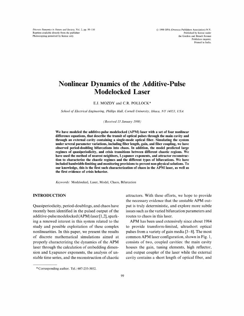
to provide transform-limited, ultrashort opticalpulses from a variety of gain media [3-8]. The mostcommon APM laser configuration, shown in Fig. 1,consists of two, coupled cavities: the main cavityhouses the gain, tuning elements, high reflector,and output coupler of the laser while the externalcavity contains a short length of optical fiber, and

100 E.J. MOZDY AND C.R. POLLOCK

NaCI ColorCenter,Crystal

T 30% ] HighCoupler Birefringent

APM LaserOutpunt Tuner Plate u,,..v.ctor 1.06 pm

Output "-ff U Nd:YAG

RBS 50% lenses Pump

AR-coated .....’xCoupling Spheres "/’. PZT-stabilized

/,Z/ High Reflector

FIGURE The NaC1 APM laser cavity.

is exactly matched in length to the main cavity.Considered alone, the main cavity is either syn-chronously pumped or actively modelocked (e.g.by an acousto-optic modulator [9]) to producerelatively long (10ps) pulses. In the APM con-figuration, a fraction of the pulsed output power iscoupled onto the optical fiber of the externalcavity, and then retroreflected back to recombinewith the pulses circulating in the main cavity. Thesmall fiber core diameter leads to high peakintensities, causing a frequency chirp due to non-linear self-phase modulation (SPM). When thelength of the external cavity is properly adjusted,the frequency-chirped pulses interfere with those ofthe main cavity constructively at the peaks, anddestructively at the wings, resulting in an effectivetemporal shortening of the pulses. After manyround trips, dispersion and finite bandwidthbalance the pulse shortening caused by this process,and the laser reaches a steady-state operating point,generating pulses on the order of 100 fs in duration.

Because modelocked lasers are characterized bya (periodic) train of pulses at the output couplerseparated by the main cavity round-trip transittime, such lasers are most easily described by aniterative model. In previous work [1], four differ-ence equations were used to model the APM laser,verify steady-state operation, optimize laser param-eters, and predict the presence of bifurcations andchaos. Despite these achievements, no one haspursued these equations in a more detailed under-standing of the APM dynamics. In particular, doquasiperiodicity and chaos truly exist in the APMlaser and if so, can the chaos be characterized by a

largest Lyapunov exponent? What is the dimen-sionality of the chaotic system, and can onereconstruct a strange attractor from the time series

output of the iterative model? What routes to chaosexist in the APM system? Although the iterativemodel has been used to suggest rich chaoticdynamics, these questions indicate the need forbetter characterization.We have pursued these questions at length, and

will describe the development and use of theiterative APM model. In determining a properembedding dimension for the chaotic dynamics,calculating a largest Lyapunov exponent, andreconstructing several different attractors fromthe output time series, we provide convincingevidence that this laser’s unstable output is trulydeterministic. We also explore the routes to chaos,which include period-doubling and crisis transi-tions in different regions of phase space.

THE APM MODEL

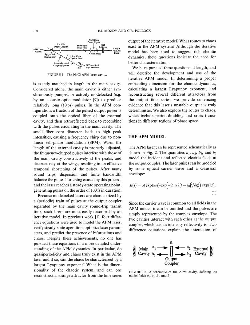
The APM laser can be represented schematically asshown in Fig. 2. The quantities al, a2, bl, and b2model the incident and reflected electric fields atthe output coupler. The laser pulses can be modeledby some optical carrier wave and a Gaussianenvelope:

/

E(t) A exp(icot)exp[-2 ln2[t- to]/St) exp(iqS).

Since the carrier wave is common to all fields in theAPM model, it can be omitted and the pulses are

simply represented by the complex envelope. Thetwo cavities interact with each other at the outputcoupler, which has an intensity reflectivity R. Twodifference equations explain the interaction of

RMain a’a2 External ICavity b b2 Cavity

OutputCoupler

FIGURE 2 A schematic of the APM cavity, defining themodel fields ax, a., bx, and b2.

NONLINEAR DYNAMICS OF THE APM LASER 101

these fields"

bl al x/ + azv/1 R, (2)

b2 al v/1 R a2x/-. (3)

The b fields generated above make a round triptraverse of their respective cavities in becoming a

fields. Defining all of the optical processes in thosetraverses allows us to develop a description of thepulse evolution which can then be iterated. FromFig. 1, the field bl passes through the birefringenttuner plate (BTP) and saturable gain twice beforereturning to the output coupler as al. The tuner

plate, positioned at Brewster’s angle (56.8) in themain cavity, has an intensity transmission thatdepends upon wavelength as [10]

The spectral filtering of the BTP and gain are

applied to the main cavity pulse in the frequencydomain by taking the product of the pulse spectrumwith both filter responses. Expressing the inputpulse to this process as p(t), the filtered outputbecomes

[’(p(t)) exp(iwt)IT G

[/_i (6)

The effect of the saturable gain can be treated inthe time domain [12]"

( )G lout//in exp + gin/gsat(7)

4 2

IT(A) sinZ(2qS) n no cOS2 0

(n2o cos2 q5 COS2 0) 2

(__{ ne[14-cs2Ocs2d/)(1/n2e-1/n2o)]x sin2

[1 cos2 0(sin2 /n2e + cos2 /n2o)] 1/2

[1 COS2 0///2o] 1/2 (4)

where go is the small-signal gain,

go exp(o-AN0), (8)

given cr 9 x 10-17 cm2, the gain cross-section forNaC1 OH-, and unsaturated population inversion

AN0, which is proportional to the pumping. Uinand Usat are input pulse and saturation energyfluences, defined as

where 0 is the angle formed by the surfaceof the plate and the cavity optic axis, b is theangular deviation of the plate’s extraordinary axisfrom the vertical, is the plate thickness, and no (ne)is the index of refraction of the (extra)ordinaryaxis. For this model, we used a plate of thicknesst-1.75 mm, which is similar to that used in thelaboratory.The laser gain both amplifies the pulse and

performs some spectral filtering, due to its finitegain bandwidth. For NaCI: OH-, the gain emissionspectrum is Gaussian in shape, with a bandwidth ofu 45 THz centered at Uo 187.5 THz (1.60 gm)[11]. Given these parameters, the normalized gainversus frequency can be expressed as

G(u) exp[-4 In 2(u ’o)2/5/’2] (5)

Uin (t) Iin(t) dt, (9)

gsat (10)

For NaCI:OH- laser centered at A= 1.60gm,Usa 1.38 mJ/cm2. With these definitions, Eq. (7)expresses the saturable gain as a function ofintracavity pulse energy, independent of gainlineshape.The overall relationship between the fields al

and bl can then be achieved by first filtering blaccording to Eq. (6), then multiplying by the one-

pass gain in Eq. (7) twice, then filtering accordingto Eq. (6) a final time.

In the external cavity, the fields a2 and b2 arerelated by propagation through the single mode


optical fiber in the external cavity. Given the fibercore radius 51am and the duration of typicalAPM laser pulses (100 fs), peak pulse intensitieswithin the fiber can exceed GW/cm2. With suchhigh intensities, the fiber exhibits an intensity-dependent index of refraction:

n(I) no + nI. (11)

This index variation causes the high-intensitycenter of the pulse to travel more slowly than theleading and trailing edges, thereby causing com-

pression (frequency upshift) of the optical carrierwave on the trailing edge, and stretching (frequencydownshift) on the leading edge. This effect is knownas self-phase modulation (SPM), and is usuallyexpressed in terms of the additional phase a pulseacquires in traveling a certain length L of fiber,

exp(-i 64)-expl-i(o)n2I(t)l. (12)

For fused silica fiber, n2 3.2 10-16 cm2/W, anda length on the order of 20 cm can typically generate7r radians of phase across a single pulse.To express the effects of SPM in this model, we

can write a2 in terms of b2 as

a2(t) Rs’7/b(t)

xexp 0+2r/0A0

(13)

where RBS is the intensity reflectivity of thebeam-splitter, 3’ is the forward fiber couplingefficiency (between cavity and fiber modes), 2 isthe back-coupling efficiency (the fraction ofthe intensity emerging from one pass through thefiber able to be coupled back onto thefiber after retroreflection), and r/0 is the char-acteristic impedance of air, about 377 f, used toconvert between field strength and intensity. Thesquare-root dependence on ")/2 in the aboveexpression results from taking the back-couplingloss only once, since none of the light is lostexiting the fiber to strike the retroreflector.

Typically, RBs=0.5, L20-50cm, 710.5-0.8, 72 0.6-0.95, and o 3.1 for stable APMoperation.

SIMULATION RESULTS

We first tested the APM model by simulating thesteady-state operation of the laser. Given Eqs. (2)and (3) which explain the recombination of pulsesal and a2, and Eqs. (6), (7), and (13) which describethe transformation of fields bl and b2 by the mainand external cavities, the model can be iteratedto generate successive a and b fields. With hundredsof round trips through the laser, steady-state isachieved for the typical range of parameters givenabove.

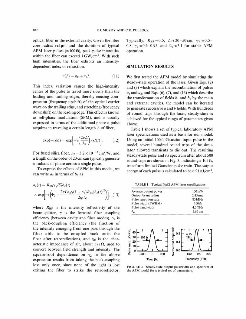
Table I shows a set of typical laboratory APMlaser specifications used as a basis for our model.Using an initial 100 fs Gaussian input pulse in themodel, several hundred round trips of the simu-lator allowed transients to die out. The resultingsteady-state pulse and its spectrum after about 500round-trips are shown in Fig. 3, indicating a 105 fs,transform-limited Gaussian pulse train. The outputenergy of each pulse is calculated to be 6.91 nJ/cm2,

TABLE Typical NaC1 APM laser specifications

Average output power 100mWOutput beam radius 2.45 mmPulse repetition rate 80 MHzPulse width (FWHM) 100 fsPulse bandwidth 4.5 THzA0 1.60 pm

40 r" ,A 1130

1 mO.8 ]---f4.15

i.’’20 0.410

0 I 0.0-200 0 200 80 190 200

Tim [fs] rclueny [THz]

FIGURE 3 Steady-state output pulsewidth and spectrum ofthe APM model for a typical set of parameters.


which corresponds to 104mW given the pulsewidth and output beam radius. The steady-stateoutput of the model is thus in excellent agreementwith the laser specifications of Table I.Having verified the accuracy of the APM model

in the steady-state, we next varied certain laserparameters, attempting to find a regime of more

complicated APM dynamics. With a fixed small-signal gain and forward and backward fibercoupling coefficients of 0.5 and 0.6, respectively,we first varied the length of the fiber from 10 cm toover 50 cm, since the fiber length is the most direct

perturbation to the SPM nonlinearity (see Eq. (13)).In varying a model parameter, we iterated themodel several hundred times after each parameteradjustment, to insure that the system had settledinto a new steady-state. Plotting about 30 succes-

sive output pulse energies for each separate fiberlength value, Fig. 4 shows that the laser exhibits

seemingly unstable behavior after a length of 27 cm.Figure 5 shows the time progression and phase-

space orbit of the output energies, with the discretedata connected for clarity. We observe that theoutput is periodic, with a period of about 17.5iterations. Since the laser output itself is periodic(a pulse train with a frequency of 80 MHz), we can

conclude that this behavior is quasiperiodic, sincethe secondary oscillation period is incommensuratewith the fundamental period. The phase-space plot,or first return map (nth versus the (n+ 1)thiteration) provides a similar conclusion since theorbit becomes continuous as n -+ oc: no two output

8.0

"7.0

t5.0

10 20 30 40 50

Fiber Length [cm]

FIGURE 4 Fiber length bifurcation diagram for moderatefiber coupling (3’1 0.5 and 72 =0.6) showing a large unstableregion.

7.2

"/.0

68

6.60 40 80

Iteration Number

7.2

"/.0

6.8

6.6

n Pulse Energy

FIGURE 5 Time series and first return map for the unstableregion of Fig. 4, demonstrating quasiperiodic output.

pulses are coincident in phase-space, indicatingtwo, incommensurate frequencies. As the fiber

length increases beyond 27cm, similar analysisshows that the output remains quasiperiodic, withthe orbit in phase-space simply becoming more

convoluted.We next repeated the fiber length variation with

increased forward and backward fiber couplingcoefficients of 0.8 and 0.9, respectively, close to theupper limit of achievable laboratory conditions.We chose to vary the coupling coefficients becausethey not only perturb the SPM, but also increasethe interference between the main and externalcavities while remaining readily adjustable labora-tory parameters. Figure 6 shows the resultingbifurcation diagram when the output pulse energiesare again plotted for each value of fiber length. Wesee the laser bifurcate from period-one to period-two behavior around 9 cm, followed by a period-doubling cascade into chaos, much like thewell-known logistic map. Figure 7 shows a close-up of the unstable region, where the chaoticbehavior suddenly drops into a stable orbit near

l-16.30cm, again period-doubles into chaos,transitions to another seemingly chaotic region,then reverse bifurcates to a stable orbit.To properly conclude that these instabilities are

indeed chaos, we sought to calculate a largestLyapunov exponent for each of the three unstableregions of Fig. 7: l 15.9-16.3 cm, l 16.67-16.76 cm, and l 16.83-17.12 cm. This involved re-

constructing the laser output in delayed-coordinatephase-space, then employing the algorithm of


5.0

4.5

4.0

35

3.0

2.5

8 10 12 14 16 18

Fiber Length [cm]

20 22

FIGURE 6 Fiber length bifurcation diagram for large fiber coupling (71 =0.8 and 72--0.9) revealing period doubling andchaos.

Fiber Length [cm]

FIGURE 7 Close-up of period-doubling and chaotic regions of the fiber length bifurcation diagram of Fig. 6.


Wolf et al. [13] to calculate the exponent. Phase-space reconstruction first requires some knowledgeof the dimensionality of the APM laser, which isreadily provided by the algorithm of Kennel et al.involving false nearest neighbors [14]. Essentially,this method determines the percent of false-nearestneighbors when the laser output is reconstructed insuccessive integer dimensions, starting from 1.High-dimension systems reconstructed in lower-dimensions will exhibit large percentages of falseneighbors, but this percentage will drop to zerowhen the proper embedding dimension is reached.Figure 8 shows the result of such a calculation foreach unstable region of Fig. 7, and the properembedding dimension is three in each case.

Knowing the proper embedding dimension, wenext reconstructed the phase-space orbits, usingn=32000 output iterations of the model for a

given set of parameters in each chaotic region, andthe delayed coordinates n, n + 1, and n + 2. Oneattractor from each region is shown in Figs. 9-11:the first two regions actually yield two attractorseach, one for each of the two major branches ofthe bifurcation diagram, while the third regionconsists of four distinct attractors, due to theunderlying period-four behavior. From a graphicalviewpoint, the orbits indeed exhibit the qualities ofstrange attractors, including low topologicaldimension and folding behavior, and self-similarstructure.

o 80-o- Regmn 3. 60 [-- , --X- Region 2

Z, 40- ’. -<y-Regionl

20 .-.6 0N 2 3 4 5

Embedding Dimension

FIGURE 8 False-nearest neighbor embedding dimensioncalculation for the three prominent regions of instability inFig. 7.

The best evidence of chaotic behavior however,lies in an estimation of the largest Lyapunovexponent. This exponent was obtained with theWolf code using a minimum initial displacement of10-5 and a "largeness" condition on the finaldisplacement of 10-2 (where the order of theattractor is 10-), allowing trajectories to divergeby three orders of magnitude before calculatinglocal exponents. Such a calculation yieldsA=0.24, A2=0.14, and /3=0.15 bits/s for therespective chaotic regions, the positive values indi-cating the presence of chaos, where nearby trajec-tories in phase-space locally diverge exponentially.

Figure 7 still raises questions as to the nature ofthe transitions between the different chaoticregions, or more generally, the routes to chaos inthe APM laser. The period-doublings provide an

obvious answer as one of the routes into eachchaotic region, but the nature of the transitions atl-- 16.3 cm where the chaos suddenly drops into a

stable orbit, and l= 16.72cm where one chaotic

region suddenly jumps to another still remainsunknown.

In order to understand these transitions, we con-sider 16 000-iteration reconstructions of the laseroutput at the critical parameter values. Figure 12shows the case of l= 16.3 cm, reconstructed threetimes with successively larger numbers of iterationsremoved from the beginning of the time series. Plot(a) shows an attractor identical to Fig. 9, from thefirst chaotic region. Plot (b), with the first 1250iterations removed, displays a much more "sparse"looking attractor. When the first 2500 iterationsare removed, plot (c) shows that the laser is actuallyexhibiting the stable periodic orbit for --, oc. Thisprogression demonstrates what is known as achaotic transient, where the system follows thenearby, destabilized chaotic attractor for somefinite number of cycles, then finally falls onto adifferent (stable) orbit. Together with the facts thatthe transition between the chaotic and stableregions is sudden and causes the destruction ofthe attractor, this chaotic transient provides con-

vincing evidence that the transition at 16.3 cm isa crisis [15].


2.9

2.8-----

2.7--

2.6---

2.5"--

2 4

n+l

FIGURE 9 Reconstructed chaotic attractor in three dimensions for l 15.9-16.3 cm.

2.8

2.75

2.7

2.65

2.85

2.752.75

n+l

2.65

2.6 2.62.65

FIGURE 10 Reconstructed chaotic attractor in three dimensions for l 16.67-16.76cm.

2.85


2.69-.

2.68-.2.67

2.65-.

/.,! ;’2.61.

2.6 -----’-

2.62 2.622.6 2.6

n+l

FIGURE 11 Reconstructed chaotic attractor in three dimensions for l 16.83-17.12cm.

2.5

2.2 2.4 2.6 2.8

n+l (a)

2.5

2.2 2.4 2.6 2.8

n+l (b)

2.5

2.2 2.4 2.6 2.8

n+l (C)

FIGURE 12 Chaotic transient in the APM output near l= 16.3cm: (a) shows iterations 1-16000 containing the large initialchaotic transient preceding a small stable orbit; (b) shows 1251-16000 where a portion of the initial chaotic transient has passed;and (c) shows 2501-16 000 where the entire chaotic transient is over, and the system has settled onto the stable orbit.


2

2.7 2.72.6 2.6

n+l

(a)

2.8

2.6 2.6n+l

(b)

2.6 2.6n+l

(c)

2.9

FIGURE 13 Chaotic transient in the APM output near l-- 16.72cm: (a) shows iterations 1-12000 with both an initial chaotictransient and two drastically different coexisting stable chaotic attractors; (b) shows 4001-12000 where a portion of the initialchaotic transient has passed; and (c) shows 8001-12000 where the system has settled onto the two stable coexisting chaoticattractors.

Likewise, we examined the sudden transition at1-- 16.72 cm, and found similar behavior. Figure 13shows the progression of the reconstructed timeseries, where a region two chaotic transient dis-appears to leave the region three attractor for

oo. This sudden change of attractor and thepresence of the chaotic transient indicate that theregion two/three transition is also a crisis.

Since adjusting the fiber couplings had a dra-mati6 effect on the fiber length bifurcation dia-gram, we decided to investigate fiber coupling asthe bifurcation parameter. For a fixed fiber lengthof 15 cm, we varied the forward and backward fibercoupling coefficients simultaneously0.1). Figure 14 shows the resulting bifurcationdiagram, which is very similar to the fiber lengthcase. Aside from variations in the absolute output

energy, the only major difference between thefiber coupling and length cases is the unstableregion beyond the second crisis at 7 =0.715. Thisregion exhibits underlying period-two instead ofperiod-four, and also does not reverse bifurcateback to a stable orbit. An embedding dimensioncalculation shows that this region should bereconstructed in four dimensions, and the resultinglargest Lyapunov exponent calculation revealsA 0.31 bits/s, again indicating chaos.Beyond fiber parameters, we also varied the

small-signal gain (which is proportional to thepumping strength in the laboratory), and foundresults similar to the fiber length case. For smallfiber coupling, the laser exhibited quasiperiodicityfor large gain, while higher coupling allowed forperiod-doubling, chaos, and crises.


5.5

5.0

4.0

3.0

2.5

FIGURE 14 Fiber coupling bifurcation diagram, which shows essentially the same features as the fiber length bifurcationdiagram.

CONCLUSIONS

Although the model described above is fairlycommon for the APM system, one should be awarethat certain effects were neglected, includingtemporal gain saturation (across the pulse profile)and dispersion. The model remains valid in a

practical sense however, since temporal gainsaturation cannot easily be observed in the labora-tory (short timescale), and generally only causes

asymmetry in the pulse shape. Moreover, the NaC1laser is usually operated with dispersion-shiftedfiber (D0 at A 1.55 gm) and dispersion can beneglected to first order.More important to the implementation of this

model were errors due to overly large bandwidth.Because some of the external cavity energy recircu-lates through the external cavity without beingfiltered by the gain and tuner plate in the maincavity, it is possible under conditions of largenonlinearity (long fiber, high coupling, large gain,etc.) for the recirculating pulses to obtain hugeamounts of chirp after many iterations, corre-

sponding to pulse bandwidths exceeding 100 THz.In the time domain, this corresponds to oscillationson the order of the optical carrier frequency

(187.5 THz), at which point the distinction betweenthe optical wave and its envelope is meaningless;i.e., the situation is non-physical.When such a situation occurs in the model, the

center of the pulses typically becomes extremelynarrow, eventually collapsing to a point disconti-nuity. This event results in a drastically alteredpulse integral (energy), and manifests itself in a

discontinuity in the bifurcation diagram. In fact,such a non-physical discontinuity in a similarmodel was erroneously reported as hysteresis [1].Experimentally, this problem would never arise,because optical components would limit the pulsebandwidth to some finite level. We chose to correctthis problem by inserting into the external cavity a

filter which approximates the finite-bandwidthcoating of a typical laboratory mirror, about100 nm.

SUMMARY

We have modeled the APM laser with a simple setof four difference equations which provide a greatamount of insight into the complex dynamics of theAPM system. In particular, the model verified


quasiperiodicity, period-doubling, and chaos in thelaser output. In addition, we explored the nature ofthe APM chaos, including the dimensionality ofthe laser dynamics, the reconstructed chaoticattractors, largest Lyapunov exponents, and crisistransitions between different chaotic regions. Ourexploration of several different parameter varia-tions should also prove useful to the developmentof laboratory experiments to verify and exploit thedynamics of the APM system.

Acknowledgements

We would like to thank A. Gavrielides, V. Kovanis,and T. Newell of Phillips Laboratory, KirtlandAFB in Albuquerque NM for useful discussion andanalysis code. This work was funded by the JointService Electronics Program, contract #F49620-96-1-0162.

References

[1] Sucha, G., Bolton, S.R., Weiss, S. and Chemla, D.S. (1996).Period doubling and quasi-periodicity in additive-pulsemode-locked lasers. Optics Letters 20, 1794-1796.

[2] Morgner, U., Rolefs, L. and Mitschke, F. (1996). Dynamicinstabilities in an additive-pulse mode-locked Nd:YAGlaser. Optics Letters 21, 1265-1267.

[3] Mollenauer, L.F. and Stolen, R.H. (1984). The soliton laser.Optics Letters 9, 13-15.

[4] Mitschke, F.M. and Mollenauer, L.F. (1986). Stabilizingthe soliton laser. IEEE Journal of Quantum ElectronicsQE-22, 2242-2250.

[5] Mark, J., Liu, L.Y., Hall, K.L., Haus, H.A. and Ippen, E.P.(1989). Femtosecond pulse generation by additive pulsemodelocking, lEE Colloquium on ’Applications of Ultra-short Pulses for Optoelectronics" 87, 66.

[6] Ippen, E.P., Haus, H.A. and Liu, L.Y. (1989). Additivepulse mode locking. Journal of the Optical Society ofAmerica B 6, 1736-1745.

[7] Yakymyshyn, C.P., Pinto, J.F. and Pollock, C.R. (1989).Additive-pulse mode-locked NaCI:OH- laser. OpticsLetters 14, 621-623.

[8] Sennaroglu, A., Carrig, T.J. and Pollock, C.R. (1992).Femtosecond pulse generation by using an additive-pulsemode-locked chromium-doped forsterite laser operated at77K. Optics Letters 17, 1216-1218.

[9] Pinto, J.F., Yakymyshyn, C.P. and Pollock, C.R. (1988).Acousto-optic mode-locked soliton laser. Optics Letters 13,383-385.

[10] Preuss, D.R. and Gole, J.L. (1980). Three-stage birefrin-gent filter tuning smoothly over the visible region:theoretical treatment and experimental design. AppliedOptics 19, 702-710.

[11] Georgiou, E., Pinto, J.F. and Pollock, C.R. (1987). Opticalproperties and formation of oxygen-perturbed F- colorcenter in NaC1. Physical Review B 35, 7636-7645.

[12] Haus, H.A. (1975). A theory of forced mode locking. IEEEJournal of Quantum Electronics 11, 323-330.

[13] Wolf, A., Swift, J.B., Swinney, H.L. and Vastano, J.A.(1985). Determining Lyapunov exponents from a timeseries. Physica D 16, 285-317.

[14] Kennel, M.B., Brown, R. and Abarbanel, H.D. (1992).Determining embedding dimension for phase-space recon-struction using a geometrical construction. Physical ReviewA 45, 3403-3411.

[15] Grebogi, C., Ott, E. and Yorke, J.A. (1983). Crises, suddenchanges in chaotic attractors, and transient chaos. PhysicaD 7, 181-200.

Submit your manuscripts athttp://www.hindawi.com

Hindawi Publishing Corporationhttp://www.hindawi.com Volume 2014

MathematicsJournal of


Mathematical Problems in Engineering

Hindawi Publishing Corporationhttp://www.hindawi.com

Differential EquationsInternational Journal of

Volume 2014

Applied MathematicsJournal of


Probability and StatisticsHindawi Publishing Corporationhttp://www.hindawi.com Volume 2014

Journal of


Mathematical PhysicsAdvances in

Complex AnalysisJournal of


OptimizationJournal of


CombinatoricsHindawi Publishing Corporationhttp://www.hindawi.com Volume 2014

International Journal of


Operations ResearchAdvances in

Journal of


Function Spaces

Abstract and Applied AnalysisHindawi Publishing Corporationhttp://www.hindawi.com Volume 2014

International Journal of Mathematics and Mathematical Sciences


The Scientific World JournalHindawi Publishing Corporation http://www.hindawi.com Volume 2014


Algebra

Discrete Dynamics in Nature and Society



Decision SciencesAdvances in

Discrete MathematicsJournal of

Hindawi Publishing Corporationhttp://www.hindawi.com

Volume 2014 Hindawi Publishing Corporationhttp://www.hindawi.com Volume 2014

Stochastic AnalysisInternational Journal of

the additive-pulse modelocked laser

Documents