Genetica 112–113: 9–32, 2001.© 2001 Kluwer Academic Publishers. Printed in the Netherlands.

9

The adaptive landscape as a conceptual bridge between micro-and macroevolution

Stevan J. Arnold, Michael E. Pfrender & Adam G. JonesDepartment of Zoology, 3029 Cordley Hall, Oregon State University, Corvallis, OR 97331, USA (Phone:(541) 737-4362; Fax: (541) 737-0501; E-mail: arnolds@bcc.orst.edu)

Key words: adaptive landscape, macroevolution, microevolution, phenotypic evolution, quantitative genetics,selection surface, selective line of least resistance

Abstract

An adaptive landscape concept outlined by G.G. Simpson constitutes the major conceptual bridge between thefields of micro- and macroevolutionary study. Despite some important theoretical extensions since 1944, this con-ceptual bridge has been ignored in many empirical studies. In this article, we review the status of theoretical workand emphasize the importance of models for peak movement. Although much theoretical work has been devoted toevolution on stationary, unchanging landscapes, an important new development is a focus on the evolution of thelandscape itself. We also sketch an agenda of empirical issues that is inspired by theoretical developments.

Introduction

Is the ‘modern synthesis’ incomplete? At the cen-ter of disenchantments with the neo-Darwinian the-ory of evolution is the connection between micro-and macroevolution. The term microevolution refersto the processes that lead to phenotypic diversific-ation among arrays of conspecific geographic racesor closely related species. Macroevolution, on theother hand, covers processes responsible for the di-vergence among genera or higher taxa. We favorthe view that neo-Darwinian theory can account forboth micro- and macroevolutionary patterns (Lande,1980a; Charlesworth, Lande & Slatkin, 1982). Nev-ertheless, despite our optimism, we recognize thatdisenchantment is easy to find in the literature of evol-utionary biology. The main complaints fall into twobroad categories: (1) claims that microevolutionaryprocesses cannot logically be extrapolated to explainmacroevolutionary pattern (Stanley, 1979; Eldredge& Cracraft, 1980), and (2) the idea that importantpattern-producing processes operate above the levelof populations (e.g., species selection; Rensch, 1959;Vrba, 1983). The conceptual chasm between micro-evolutionary processes (inheritance, selection, drift)

and macroevolutionary patterns appears to some au-thors to be deep, wide and unbridgeable. Remarkably,a conceptual bridge was outlined more than 50 yearsago by Simpson (1944, 1953) but is neglected by manyevolutionary biologists today.

Simpson (1944) boldly used an adaptive land-scape to synthesize genetical and paleontologicalapproaches to evolution. In Simpson’s conceptualiz-ation a two-dimensional space represents the possiblecombinations of two phenotypic characters (structuralvariants). Elevation contours on this space representpopulation fitness (adaptiveness). Using this pheno-typic landscape, Simpson illustrated the concepts ofphenotypic variation, selection, immediate responsesto selection, long-term evolutionary trends, speciation,and adaptive radiation. No visualization before orsince 1944 has been so successful in integrating themajor issues and themes in phenotypic evolution.

Topographic simplicity and peak movement arenotable features of Simpson’s landscapes. He usuallyportrayed just one or two adaptive peaks. Peak move-ment is a second important theme. Simpson modeledthe tempo and mode of evolution with various patternsof peak bifurcation and movement. In Simpson’s con-ceptualization the population evolves in relation to a

10

changing landscape. The model is not one of evolutionon a complex but stationary landscape. In recent years,the theoretical literature has explored the issue of peakmovement. This change in focus from stationary toevolving landscapes is so profound that it is fair tocall it a paradigm shift, yet it has escaped the noticeof many evolutionary biologists. We shall return to thethemes of topographic simplicity and peak movementlater in our discussion.

The landscape under discussion should not be con-fused with certain other landscape concepts in theliterature of evolutionary biology. The landscape thatSimpson used, and which we will explore, is a spaceof phenotypic characters (Lande, 1976a, 1979). El-evation on this space reflects population-level fitness(adaptation). This phenotypic landscape is a directdescendant of Wright’s adaptive landscape (Wright,1931, 1932, 1945), except that his landscape is a spaceof gene frequencies (Wright, 1932, 1982; Provine,1986). In Wright’s conceptualization, the landscapeis complex (due to epistasis in fitness) and largelystationary. Movement on the Wrightian landscape rep-resents evolutionary change in gene frequencies ratherthan phenotypic evolution per se. Other landscapes arestill more distant to the one under discussion. Rice(1998) uses a landscape to model the evolution ofphenotypic plasticity in which elevation represents acharacter and the axes reflect underlying factors. Wad-dington’s (1957) epigenetic landscape is a space ofabstract variables that is used to describe the modaldevelopmental tendency and major deviations from it.

In evolutionary biology today Simpson’s landscapeis not routinely used to motivate empirical work, eventhough its power has been confirmed and extended bytheoretical studies. The theoretical developments arerelatively recent, tracing back to Lande (1976a, 1979),and are often couched in the language of multivariatecalculus and linear algebra. Simpson’s landscape livesand flourishes in these theoretical papers, but rarelyis illustrated. Consequently, the idea that Simpson’slandscape is the major conceptual bridge between thefields of micro- and macroevolution is unappreciatedby many evolutionary biologists. The goal of this art-icle is to give an overview of theoretical developmentsin the field of phenotypic evolution, especially thosethat can be visualized with Simpson’s landscape. Ourthesis is that these results and visualizations could andshould guide empirical work in a wide variety of dis-ciplines. Our survey also highlights some directionsthat need theoretical exploration. The bridge is stillunder construction.

Some recent works are important companions toour discussion. Hansen and Martins (1996), build-ing on the work of Felsenstein (1973, 1985), havepointed out that the fields of systematics, evolutionarygenetics, and comparative biology rest on a commonset of equations relating evolutionary pattern (traitvariance and covariance among taxa) to process (muta-tion, selection, drift). Those unifying equations arein turn based on models that relate microevolutionto macroevolution. In this review we give a land-scape visualization of the various process models thatare central to Hansen and Martins’ (1996) discussion.Schluter (2000) has used Simpson–Lande landscapesto illustrate the concept of adaptive radiation and tosurvey the growing empirical literature. We will relyon Schluter’s (2000) treatment of adaptive radiations,while extending his discussion of landscapes and howthey can be used. To provide a connection to thetheoretical literature, while keeping the text free ofmathematical notation, we will indicate equations bynumber in parenthesis. The corresponding mathemat-ical expressions and their attributions are given in theAppendix.

Current conceptualizations of theadaptive landscape

Overview

The adaptive landscape for continuously distributed,phenotypic characters is a surface that relates averagefitness to average character values. Although only theone character case is usually portrayed in textbooks,the landscape must be visualized in at least two di-mensions to appreciate fully the key concepts. Thelandscape is more than a theoretical construct – crucialfeatures of this surface can be determined empirically.

In this section, and the ones to follow, we will usea landscape concept in which selection favors an in-termediate optimum. There are many reasons for thischoice for selection, and chief among them is its firmempirical foundation. This form of selection (some-times called stabilizing or centrifugal selection) wasdocumented in some of the earliest empirical studiesof phenotypic selection (Karn & Penrose, 1951) andhas been found in many subsequent studies (Endler,1986; Kingsolver et al., 2001). Stabilizing selectioncan produce a persistent equilibrium, a result thatappeals to many naturalists, in contrast to linear se-lection regimes under which populations are perpetu-ally subjected to directional change. Long-maintained

11

stabilizing selection can explain such diverse phenom-ena as character canalization, geographic variation,and transgressive segregation in second-generation hy-brids resulting from a wide cross (i.e., the appearanceof variants outside the range of the parental popu-lations) (Mather, 1941, 1943; Schmalhausen, 1949;Wright, 1968; Rieseberg, Archer & Wayne 1999). Fur-thermore, directional selection can be accommodatedin theoretical work by simply shifting the selective op-timum away from the character mean (Lande, 1976a).Although we have chosen to illustrate the landscapeconcept with stabilizing selection, other modes of se-lection are feasible and the sections that follow couldbe revisited using those alternative selection modes.In particular, a recent review of the selection literat-ure discovered that instances of disruptive selectionwere as common as stabilizing selection (Kingsolveret al., 2001), a result that challenges our emphasison stabilizing selection. Univariate studies of selec-tion predominated in that review, so the jury is stillout on whether the adaptive landscape is commonlyhill, pit, saddle or ridge-shaped (Phillips & Arnold,1989).

The adaptive landscape for a single character: themarch of the frequency distribution

The adaptive landscape for a single character understabilizing selection can be represented by a dome-shaped curve. If the mean of the character is situatedsome distance from the apex (optimum) of the curve,the population experiences directional selection thatwill tend to shift the mean toward the optimum if thecharacter is heritable. If heritability is constant, theamount of change across generations is proportionalto the distance to the optimum (Lande, 1976a). Evol-ution towards a stationary optimum is rapid at first,decelerates as the mean approaches the optimum, andthen ceases entirely when the mean coincides with theoptimum (Figure 1), (1). In other words, the frequencydistribution marches until it lies under the peak of thelandscape. This march corresponds to a progressive in-crease in average fitness, ceasing when the populationachieves a fitness maximum directly under the peak(Lande, 1979), (2). In ecological terms, the movementof the optimum away from the character mean mightcorrespond to a change in climate, resources, predatorsor change in any other set of conditions that inducesdirectional selection. The movement might happen in-stantaneously and then cease. An ecologically moreplausible circumstance is that the peak movement con-

Figure 1. An adaptive landscape for a single character under sta-bilizing selection (a). The natural logarithm of mean populationfitness is shown as a function of phenotypic mean. Evolution ofthe distribution of phenotypic values in response to the adaptivelandscape (b).

tinues over a period of generations so that for someperiod of time the population chases an ever-movingoptimum. Thus, during the Pleistocene, most periodsof, say, a hundred generations might have been char-acterized by progressive change in temperature that inturn induced continued change in a host of ecologicalvariables affecting fitness. For any particular charac-ter this progressive change translates into an optimumthat moves steadily away from the mean in the samedirection. Colonization of a new environment can alsocreate a situation in which the trait mean is some dis-tance from the optimum with resulting rapid evolution.Colonization of new hosts, new spawning habitats andenvironments with new predators are examples (Via,1991; Reznick et al., 1997; Feder, 1998; Hendry et al.,2000).

A stationary adaptive landscape for two characters:the simplest case of multivariate evolution

The adaptive landscape for two characters under sta-bilizing selection can be represented by a hill-shapedtopography. The optimum is represented by the crestof the hill. If the bivariate character mean is locatedsome distance from the optimum, the population ex-periences directional as well as stabilizing selection.The strength of directional selection corresponds tothe direction of steepest uphill slope from the char-acter mean on the adaptive landscape (Lande, 1979),(3). This vector can be resolved into two compon-ents or selection gradients, corresponding to the twocharacter dimensions (Figure 2). A steeply slopinghill represents strong directional selection, whereas a

12

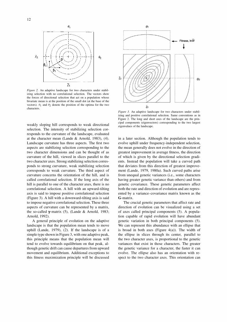
Figure 2. An adaptive landscape for two characters under stabil-izing selection with no correlational selection. The vectors showthe forces of directional selection that act on a population whosebivariate mean is at the position of the small dot (at the base of thevectors). θ1 and θ2 denote the position of the optima for the twocharacters.

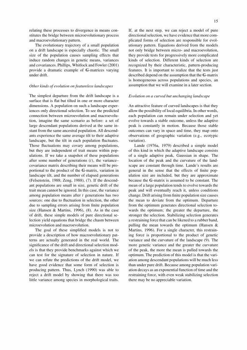
weakly sloping hill corresponds to weak directionalselection. The intensity of stabilizing selection cor-responds to the curvature of the landscape, evaluatedat the character mean (Lande & Arnold, 1983), (4).Landscape curvature has three aspects. The first twoaspects are stabilizing selection corresponding to thetwo character dimensions and can be thought of ascurvature of the hill, viewed in slices parallel to thetwo character axes. Strong stabilizing selection corres-ponds to strong curvature, weak stabilizing selectioncorresponds to weak curvature. The third aspect ofcurvature concerns the orientation of the hill, and iscalled correlational selection. If the long axis of thehill is parallel to one of the character axes, there is nocorrelational selection. A hill with an upward-tiltingaxis is said to impose positive correlational selection(Figure 3). A hill with a downward-tilting axis is saidto impose negative correlational selection. These threeaspects of curvature can be represented by a matrix,the so-called γγγ-matrix (5), (Lande & Arnold, 1983;Arnold, 1992).

A general principle of evolution on the adaptivelandscape is that the population mean tends to moveuphill (Lande, 1979), (2). If the landscape is of asimple type shown in Figure 3, with one adaptive peak,this principle means that the population mean willtend to evolve towards equilibrium on that peak, al-though genetic drift can cause departures from upwardmovement and equilibrium. Additional exceptions tothis fitness maximization principle will be discussed

Figure 3. An adaptive landscape for two characters under stabil-izing and positive correlational selection. Same conventions as inFigure 2. The long and short axes of the landscape are the prin-cipal components (eigenvectors) corresponding to the two largesteigenvalues of the landscape.

in a later section. Although the population tends toevolve uphill under frequency-independent selection,the mean generally does not evolve in the direction ofgreatest improvement in average fitness, the directionof which is given by the directional selection gradi-ents. Instead the population will take a curved paththat deviates from this direction of greatest improve-ment (Lande, 1979, 1980a). Such curved paths arisefrom unequal genetic variances (i.e., some charactershaving greater genetic variance than others) and fromgenetic covariance. These genetic parameters affectboth the rate and direction of evolution and are repres-ented by a variance–covariance matrix known as theG-matrix.

The crucial genetic parameters that affect rate anddirection of evolution can be visualized using a setof axes called principal components (5). A popula-tion capable of rapid evolution will have abundantgenetic variation in both principal components (5).We can represent this abundance with an ellipse thatis broad in both axes (Figure 4(a)). The width ofthe ellipse in slices through its center, parallel tothe two character axes, is proportional to the geneticvariances that exist in those characters. The greaterthe genetic variance for a character, the faster it canevolve. The ellipse also has an orientation with re-spect to the two character axes. This orientation can

13

Figure 4. Bivariate distributions of breeding (additive genetic) val-ues representing different patterns of genetic variance and covari-ance. (a) Large genetic variance in trait 1, small genetic variance intrait 2 and no genetic covariance. (b) Positive genetic covariance. (c)Negative genetic covariance.

be represented by the long axis of the ellipse (i.e., theeigenvector corresponding to the largest eigenvalue ofthe G-matrix). When the long axis is parallel to oneof the character axes (Figure 4(a)), there is no geneticcovariance between the two characters. An upward-tilting axis corresponds to positive genetic covariance(Figure 4(b)); a downward-tilting axis correspondsto negative genetic covariance (Figure 4(c)). The tiltof the genetic variation axis (genetic covariance) cangreatly affect the population’s response to the adaptivelandscape.

One way of appreciating the effect of genetic cov-ariance is to ask, ‘under what conditions will the pop-ulation evolve in the same direction as the directionspecified by the directional selection gradients?’ Inother words, under what conditions will the populationevolve in a straight line rather than on a curved path

Figure 5. Evolution on an adaptive landscape depends on the align-ment of the axes (principal components) of genetic variation (shadedellipses) with the axes (principal components) of the adaptive land-scape. Evolution follows straight trajectories when major (lowerleft) or minor (lower right) axes are aligned. In general, axes areout of alignment (upper left) and evolution follows a curved traject-ory. The small ellipses around each of the three population meansrepresent genetic variation around each mean (the eigenvectors andeigenvalues of the G-matrix) and hence are on a different scale ofmeasurement.

that deviates from the direction of greatest improve-ment in fitness? The answer is that the populationwill evolve in a straight line when an axis of geneticvariation is aligned with an axis of the landscape andhence with the selection gradient. Evolution will berapid when the major axis (first principal compon-ent) is aligned (Figure 5(a)) and slow when the minoraxis (second principal component) is aligned (Figure5(b)). The population will tend to evolve on a curvedpath whenever the axes of genetic variation and thelandscape are out of alignment (Figure 5(c)).

The adaptive landscape in more than two characterdimensions

No additional concepts are needed to specify an adapt-ive landscape for three or more characters, althoughthe landscape does become progressively more diffi-cult to visualize. The landscape for three charactersunder stabilizing selection, for example, can be visual-ized as a nested series of spheres or ellipsoids (Phillips& Arnold, 1989).

14

Models for the evolution of the optimum:macroevolution pattern from microevolutionaryprocess

Overview

Models for the movement of the peak of the adaptivelandscape can be used to describe changing ecologicalopportunity or temporal change in the environment.The most successful models of this kind make pre-dictions about macroevolutionary pattern from themicroevolutionary processes of selection, drift andinheritance. Because these models characterize ex-pected evolutionary patterns in statistical terms, theycan be used to test alternative visions of the adaptivelandscape. We will review these characterizations andoutline progress in using them to construct tests for thecauses of evolutionary pattern.

The following discussions of models follow a com-mon format.

(1) A microevolutionary process model is specified.The specification corresponds to assumptionsabout the adaptive landscape and inheritance.

(2) Using this model, we present expressions for theexpected variances and covariances among popula-tions or other taxa for a set of traits. This approachassumes a phylogeny for the populations. Thephylogeny that makes the models most tractableis a star, in which all populations diverge simul-taneously from one ancestor and are viewed aftersome number of generations.

(3) Alternative models for process are distinguishedby comparing their predictions about pattern(among-population variances and covariances).

To test alternative process with real data, the as-sumption of a star phylogeny can be relaxed usingan estimate of phylogeny with branch lengths thatare proportional to elapsed time. Using those branchlengths, the expected pattern across the whole phylo-geny can be calculated (Hansen & Martins, 1996;Martins & Hansen, 1996; Hansen, 1997).

Evolution on static landscapes

The following models consider evolution on land-scapes that do not change over time. While less real-istic than other models in which the adaptive landscapeitself evolves, these models provide important null hy-potheses against which to test empirical observations.

Multivariate drift: evolution on a flat landscape

The default topography for the adaptive landscape isa flat and level surface, the drift landscape. Selec-tion does not affect the evolution of the populationmean, which instead evolves in a trajectory that canbe described by Brownian movement. Because of thesimplicity of drift, we can predict the average evol-utionary outcome. That outcome depends on elapsedtime, effective population size, and the matrix of ge-netic variances and covariances (the G-matrix; Lande,1976a, 1979). Imagine a set of replicate populationsderived instantaneously from the same ancestral pop-ulation and diverging under drift alone. After anynumber of generations the expected character meanof all these descendant populations will be the sameas the original, ancestral mean. The expectation isthat drift will not change the character mean. Eventhough the average population should have the samemean as its ancestor, divergence among populationsin mean can be appreciable and will show a charac-teristic pattern. The variance–covariance matrix forthe means of descendant populations will be propor-tional to the G-matrix (Figure 6). Variance amongpopulations will also be proportional to the num-ber of elapsed generations and inversely proportionalto average effective population size (6). Thus, on adrift landscape, the G-matrix and effective populationsize encapsulate, respectively, the microevolutionaryprocesses of inheritance and drift. The equation (6)

Figure 6. Bivariate drift on a flat adaptive landscape. The smallellipse at the center represents the G-matrix of the ancestral popula-tion. The large, outer ellipse represents 95% confidence ellipse forthe means of replicate, descendant populations. Solid curved linesshow representative evolutionary trajectories. Other conventions asin Figure 5.

15

relating these processes to divergence in means con-stitutes the bridge between microevolutionary processand macroevolutionary pattern.

The evolutionary trajectory of a small populationon a drift landscape is especially chaotic. The smallsize of the population causes sampling effects thatinduce random changes in genetic means, variancesand covariances. Phillips, Whitlock and Fowler (2001)provide a dramatic example of G-matrices varyingunder drift.

Other kinds of evolution on featureless landscapes

The simplest departure from the drift landscape is asurface that is flat but tilted in one or more characterdimensions. A population on such a landscape exper-iences only directional selection. To see the predictedconnection between microevolution and macroevolu-tion, imagine the same scenario as before: a set oflarge descendant populations derived at the same in-stant from the same ancestral population. All descend-ants experience the same average tilt to their adaptivelandscape, but the tilt in each population fluctuates.Those fluctuations may covary among populations,but they are independent of trait means within pop-ulations. If we take a snapshot of these populationsafter some number of generations (t), the variance–covariance matrix describing their means will be pro-portional to the product of the G-matrix, variation inlandscape tilt, and the number of elapsed generations(Felsenstein, 1988; Zeng, 1988), (7). If the descend-ant populations are small in size, genetic drift of thetrait mean cannot be ignored. In this case, the varianceamong population means after t generations has twosources: one due to fluctuation in selection, the otherdue to sampling errors arising from finite populationsize (Hansen & Martins, 1996), (8). As in the caseof drift, these simple models of pure directional se-lection yield equations that bridge the chasm betweenmicroevolution and macroevolution.

The goal of these simplified models is not toprovide a description of how macroevolutionary pat-terns are actually generated in the real world. Thesignificance of the drift and directional selection mod-els is that they provide benchmarks against which wecan test for the signature of selection in nature. Ifwe can refute the predictions of the drift model, wehave good evidence that some form of selection isproducing pattern. Thus, Lynch (1990) was able toreject a drift model by showing that there was toolittle variance among species in morphological traits.

If, at the next step, we can reject a model of puredirectional selection, we have evidence that more com-plicated forms of selection are responsible for evol-utionary pattern. Equations derived from the modelsnot only bridge between micro- and macroevolution,they provide tests for progressively more complicatedkinds of selection. Different kinds of selection arerecognized by their characteristic, pattern-producingfeatures. It is important to realize that the tests justdescribed depend on the assumption that the G-matrixis homogeneous across populations and species, anassumption that we will examine in a later section.

Evolution on a curved but unchanging landscape

An attractive feature of curved landscapes is that theyallow the possibility of local equilibria. In other words,each population can remain under selection and yetevolve towards a stable outcome, unless the adaptivepeak is constantly in motion. Because those stableoutcomes can vary in space and time, they map ontoobservations of geographic variation (e.g., ecotypicvariation).

Lande (1976a, 1979) described a simple modelof this kind in which the adaptive landscape consistsof a single adaptive peak, Gaussian in shape. Thelocation of the peak and the curvature of the land-scape are constant through time. Lande’s results aregeneral in the sense that the effects of finite pop-ulation size are included, but they are approximatebecause the G-matrix is assumed to be constant. Themean of a large population tends to evolve towards thepeak and will eventually reach it, unless conditionschange. Drift arising from finite population size causesthe mean to deviate from the optimum. Departurefrom the optimum generates directional selection to-wards the optimum; the greater the departure, thestronger the selection. Stabilizing selection generatesa restraining force that can be likened to a rubber band,pulling the mean towards the optimum (Hansen &Martins, 1996). For a single character, this restrain-ing force is proportional to the product of geneticvariance and the curvature of the landscape (9). Themore genetic variance and the greater the curvatureof the peak, the more the mean is pulled towards theoptimum. The prediction of this model is that the vari-ation among descendant populations will be much lessthan under pure drift. Because among population vari-ation decays as an exponential function of time and therestraining force, with even weak stabilizing selectionthere may be no appreciable variation.

16

Adaptive landscapes with two stationary peaks(Felsenstein, 1979) have been used to model speci-ation and punctuated equilibria. These models are thephenotypic analog of Wright’s shifting balance theory(Wright, 1932, 1940) in the sense that a populationcan become trapped on a peak that is lower than anadjacent peak. The models are commonly called ‘peakshift’ models, but the peaks do not move. Instead, thepopulation mean shifts from one peak to the other.Peak shift models incorporate random genetic drift asa mechanism that enables the population to escapefrom a local peak. Lande’s (1986) review summarizesresults from several models, some of which are sur-prising. Under a wide range of conditions, populationsshow a pattern of relative stasis in which the pheno-typic mean erratically drifts in the immediate vicinityof one peak for a long period of time. The averagelength of this period of relative stasis (the expectedtime until the population shifts to the other peak) islong if the population is large, the original peak ishigh, and the valley between the peaks is deep (11).Surprisingly, the expected time until a shift is almostindependent of the distance between the two peaks. Ifwe focus on those rare events in which the mean shiftsto the second peak, we find that the transit down to thevalley – against the force of directional selection – isjust as fast as the transit back up to an adaptive peak.This unexpected result is a consequence of samplingrare events in which peak shifts occur. Only especiallyrapid instances of drift are included in the sample, andin these the speed of downhill transit is just as rapid asthe episode of uphill transit. Despite their simplicity,peak shift models produce an evolutionary tempo inwhich long periods of relative stasis are punctuatedby rapid evolutionary transitions. Lande (1986) andother authors of peak shift models have argued per-suasively that the conditions underlying these modelsare more plausible than the set of assumptions in-voked by Gould and Eldredge (1977). Models withtwo stationary peaks have also been used to explorethe interaction between selection and gene flow. Insuch models, gene flow from an adjacent populationcan cause a population to equilibrate downslope fromits adaptive peak (Garcia-Ramos & Kirkpatrick, 1997;Hendry, Day & Taylor, 2001).

Evolution of curved landscapes

In all the preceding models, we imagined that the ad-aptive landscape was invariant through time. We nowconsider the possibility that the landscape itself can

change. One important kind of change is caused bydensity-dependent selection, which can cause a peakto flatten as the population evolves towards it (Brown& Vincent, 1992; Schluter, 2000). In this section, how-ever, we will focus on change that involves the positionof the optimum. A simple kind of landscape evolutionis for the position of the optimum to change while thecurvature and orientation of the surface remains con-stant. We will discuss five models for peak movementthat all share the characteristic that peak shape andorientation remain constant.

Random movement

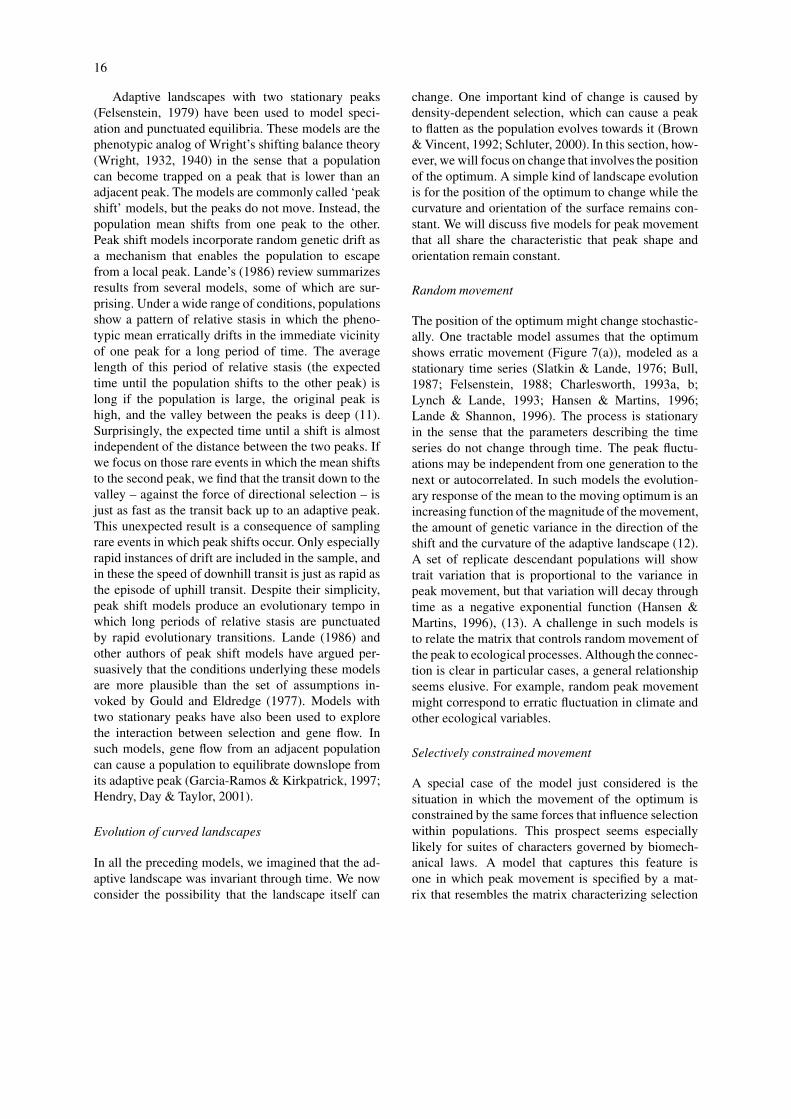
The position of the optimum might change stochastic-ally. One tractable model assumes that the optimumshows erratic movement (Figure 7(a)), modeled as astationary time series (Slatkin & Lande, 1976; Bull,1987; Felsenstein, 1988; Charlesworth, 1993a, b;Lynch & Lande, 1993; Hansen & Martins, 1996;Lande & Shannon, 1996). The process is stationaryin the sense that the parameters describing the timeseries do not change through time. The peak fluctu-ations may be independent from one generation to thenext or autocorrelated. In such models the evolution-ary response of the mean to the moving optimum is anincreasing function of the magnitude of the movement,the amount of genetic variance in the direction of theshift and the curvature of the adaptive landscape (12).A set of replicate descendant populations will showtrait variation that is proportional to the variance inpeak movement, but that variation will decay throughtime as a negative exponential function (Hansen &Martins, 1996), (13). A challenge in such models isto relate the matrix that controls random movement ofthe peak to ecological processes. Although the connec-tion is clear in particular cases, a general relationshipseems elusive. For example, random peak movementmight correspond to erratic fluctuation in climate andother ecological variables.

Selectively constrained movement

A special case of the model just considered is thesituation in which the movement of the optimum isconstrained by the same forces that influence selectionwithin populations. This prospect seems especiallylikely for suites of characters governed by biomech-anical laws. A model that captures this feature isone in which peak movement is specified by a mat-rix that resembles the matrix characterizing selection

17

Figure 7. Models for the movement of the optimum of an adaptive landscape for two characters under stabilizing selection. (a) Random,stochastic movement of the optimum. (b) Constant rate and direction of movement of the optimum, after a period of relative stasis. (c) Episodicmovement of the optimum separated by periods of relative stasis. (d) Divergence in optima, corresponding to ecological speciation.

acting within populations (14). The situation is ana-logous to the drift landscape in which a matrix thatis proportional to the G-matrix governs the drift ofthe mean. One possibility is that a matrix that is in-versely proportional to the γγγ-matrix (which specifiesthe curvature and orientation of the adaptive land-scape) governs movement of the optimum. Under thismodel the optimum undergoes random movement, butthat movement is selectively constrained. A predictionof this model is that the pattern of character meanswill be aligned with the axes of the adaptive landscape(Figure 8). If the γγγ-matrix is the same across popula-tions, the variance–covariance matrix for the means ofreplicate, descendant populations will be proportionalto the inverse of the γγγ-matrix. That among-populationvariation will, however, decay as an exponential func-tion of time. The weaker the stabilizing selection, themore variation will be retained at any given time. Con-versely, strong stabilizing selection will hasten the lossof among- population variation (14).

Constant rate and direction of movement

The optimum might move in characteristic direction ata constant rate (Figure 7(b))(Charlesworth, 1993a,b;

Lynch & Lande, 1993; Lande & Shannon, 1996).This kind of deterministic model might correspondto a constant change in climate, which translatesinto a steady change in selection pressure. Modelsof this kind can account for long-sustained evolution-ary trends that happen in parallel in multiple lineages.Kurtén (1959), for example, discusses such a patternin the evolution of mammalian body size during thePleistocene. On a shorter timescale, this model pre-dicts rapid, evolutionary response of the kind thathas been documented in response to anthropogenicchanges in the environment (Thompson, 1998; Hendry& Kinnison, 1999; Reznick & Ghalambor, 2001).Depending on the rapidity of change in selection pres-sures, these rapid responses might also correspond tothe following model.

Episodic movement

The optimum might remain relatively constant andthen rapidly move to a new position (Figure 7(c)).In Gould and Eldredge’s (1977) terminology, peakstasis might be punctuated by periods of rapid move-ment. Unlike Gould and Eldredge’s model of punctu-ated equilibrium, however, we are not supposing that

18

Figure 8. The relationship between the individual selection surface(a) and the adaptive landscape (c). The relationship between thesetwo surfaces can be visualized by averaging the individual selectionsurface (a) over the phenotypic distribution (solid curve in middlepanel) in the interval between the two vertical dashed lines. Thataveraging produces the solid dot shown in the lower panel. Slidingthe phenotypic distribution to the right, and repeating the averagingprocess at each new position, produces the curve shown in the lowerpanel, the adaptive landscape.

speciation accompanies periods of peak movement.Our model addresses change within lineages ratherthan cladogenesis. Episodic movement of the peakmight correspond to sudden invasion by a competingspecies or predator, geological or climatic cataclysm(volcanic eruption, meteor impact, etc.), colonizationof a new environment, or anthropogenic change in theenvironment.

Hansen and Martins (1996) have modeled changesin phenotypic mean that can be related to this kind ofwithin-lineage, episodic peak movement. The para-meters in their model, however, are not transparentfunctions of underlying processes of selection, driftand inheritance. Nevertheless, their model predictsthat variation among the means of descendant popula-tions is unlikely to be normally distributed. That resultmay provide a method that could be used to discrim-inate between continuous and episodic change in theadaptive landscape. Hansen (1997) models the vari-ation that is expected among species when a slightly

varying optimum moves to a new position. He alsoprovides a worked example showing how phylogenycan be incorporated into the estimation of the two peakpositions.

Population extinction is a possible response tomovement of the adaptive peak. One way to assess therisk of extinction is to calculate the total genetic loadon a population, which is the expected loss in averagefitness due to genetic and other factors. Under weakstabilizing selection, the impact of peak movement ongenetic load increases as the square of the distancethat the peak moves (Lande & Shannon, 1996), (15).Thus, large peak movements are especially likely tocause population extinction. Likewise, rapid move-ment of the peak may have a profound effect onpopulation persistence. Populations are limited in theirrate of evolutionary response to changing conditionsby the patterns of genetic variation and covariationfor characters under selection. Rapid peak movementsmay exceed the maximum rate of possible evolutionand lead to population extinction (Lynch & Lande,1993). Population and species differences in geneticarchitecture will lead to varying capacities to respondto changing landscapes. This process may contributeto macroevolutionary patterns of differential successthat some authors have labeled species level selection(Vrba, 1983).

From models for the evolution of the optimum to testsfor the causes of evolutionary pattern

A current empirical challenge is to use the models justdescribed to test for alternative causes of evolution-ary pattern. From this standpoint, the most successfulmodels are those that relate trait variance/covarianceamong related taxa to measurable, microevolution-ary processes such as selection or inheritance. Thus,the drift model predicts that among species covari-ance will be proportional to the G-matrix, whereasthe model of selectively constrained peak movementpredicts proportionality to the inverse of the γγγ-matrix.

Although we have some useful models, much the-oretical work remains to be done. A major challengeon the theoretical side is to produce models that yieldthe most common kinds of patterns in species means.One such common pattern is a correlation in the spe-cies means for two variables (e.g., brain weight andbody weight). A model of bivariate drift can producesuch a pattern (6), but the predicted correlation un-der that model is likely to be smaller than the onethat is commonly observed (Lande, 1979). Models of

19

flat, tilted landscapes predict patterns of covariancethat continually increase through time (7, 8). Modelsof curved landscapes in which the peak moves ran-domly about a fixed point predict a steady decay inthe covariance of species means (10, 13, 14). None ofthese models predict a stable pattern of interspecificcovariation. In other words, we have an infrastruc-ture for a bridge from microevolutionary process tomacroevolutionary pattern, but the construction of thebridge is far from complete. One promising directionmight be to build models of peak movement that in-clude ridges, and other channels of movement, thatare capable of yielding correlations in species means.Gavrilets (1997) makes a similar point in discussingWrightian landscapes for genotypic space.

Another way to test the models is to use their pre-dictions concerning the decay in covariance betweenspecies as a function of evolutionary distance. Somemodels predict linear decay, while others predict expo-nential decay (Hansen & Martins, 1996). Additionaltheoretical development may facilitate tests of bothkinds. For example, if the models can be arranged in ahierarchy so that each successive model differs froma simpler one by a single parameter, then it shouldbe possible to use likelihood ratios to test and rejectmodels in sequence. That goal has not been achievedbut it is not far off (Hansen & Martins, 1996).

Empirical characterization of the adaptivelandscape

Overview

Key features of the adaptive landscape can be estim-ated by analyzing variation within populations. In thenext sections we describe why such analyses are bestpursued as a multivariate problem. We review theconnection between a surface that can be estimatedfrom within-population data and the adaptive land-scape. Using this connection, we stress the importanceof estimating both the curvature and the slope of theadaptive landscape. The parameters that describe slopeand curvature are also measures of selection intensityin equations for evolutionary change.

The one character case

The analysis of selection on a single character is de-ceptively simple. Change in the mean can be used asan indication of directional selection, and change inthe variance can be used as an indication of stabilizing

or disruptive selection. The problem with such ana-lysis is that the observed shift in the mean may be aconsequence of selection on the character in question(direct selection) or it may be a consequence of selec-tion on correlated characters (indirect selection), (16).Likewise, the observed change in variance (and covari-ance) may be due to direct or indirect selection (17).Even directional selection on the character in questioncan cause its variance to contract. For all these reasons,the measurement of selection is a multivariate problem(Lande & Arnold, 1983).

Multivariate selection

The best data for sorting out direct and indirect ef-fects of selection are longitudinal data in which weknow the values for a set of phenotypic traits for eachindividual in a large sample and each individual’s fit-ness. With such data we can use multivariate statisticalmethods to characterize the surface that relates indi-vidual fitness to individual phenotypic values (Lande& Arnold, 1983). This individual selection surface isnot the same as the adaptive landscape, but it is closelyrelated to it (Kirkpatrick, 1982; Phillips & Arnold,1989; Whitlock, 1995; Schluter, 2000, pp. 85–88).Under certain assumptions we can use our character-ization of the individual selection surface to estimatekey features of the adaptive landscape. In particular,we can use this correspondence between surfaces toestimate the slope and curvature of the adaptive land-scape in the vicinity of the population’s phenotypicmean.

What is the individual selection surface and howis it related to the adaptive landscape? The individualselection surface is a surface of expected fitness foran individual as a function of the values of its phen-otypic characters (18). The relationship between thisselection surface and the adaptive landscape is simpleif the characters follow a multivariate normal dis-tribution. Under this assumption, the slope of theadaptive landscape is equal to the average slope of theindividual selection surface, weighted by the trait dis-tribution (19). The same kind of equivalency holds forthe curvatures of the two surfaces (Lande & Arnold,1983), (20). Thus, if the individual selection surface iswavy, so that slope and curvature vary with position intrait space, the adaptive landscape will have the sameaverage slope and curvature (weighted by the phen-otypic distribution), but will be smoother (Figure 8).These equivalencies can be used to estimate the de-scriptive parameters of the adaptive landscape from

20

data on individual fitness and trait values. The first stepis to characterize the individual selection surface.

Multiple regression can be used to characterize theindividual selection surface (Lande & Arnold, 1983;Phillips & Arnold, 1989; Brodie, Moore & Janzen,1995; Janzen & Stern, 1998). In such an analysis amodel is fitted so that individual fitness is predictedfrom the values of the various characters that aremeasured. Although such analyses are common in theliterature, investigators usually fit only a linear re-gression. The coefficients that are estimated by linearregression are the average slopes of the surface (β1, β2,etc.), which are equivalent to the slope of the adaptivelandscape if the traits are multivariate normal. To fita curvilinear regression – so that the curvature andorientation of the surface can be estimated, as wellas its slope – one needs to estimate the coefficientsfor squared and product variables (e.g., z2

1, z1z2). Thecoefficients for these curvilinear terms (e.g., γ11, γ12)are the elements in the γγγ-matrix (4). Such a curvilinearregression is known as a quadratic surface (18). Ex-amples of such quadratic surfaces are given in Arnold(1988) and Brodie (1992).

An unfortunate trend in the empirical literature hasbeen to estimate β coefficients and ignore γ coeffi-cients. The trend is unfortunate because γγγ plays aneven larger role in evolutionary theory than does βββ.The large role of γγγ can be appreciated by scanning theAppendix. Because γγγ describes the curvature of theadaptive landscape, it occurs in many equations thatdescribe the pattern of dispersion of species means,and how that pattern changes through time.

In addition to being descriptors of the adaptivelandscape, the β and γ coefficients have anothersignificance. The parameters corresponding to thesecoefficients are the measures of selection intensitythat appear in equations for the evolutionary changein the phenotypic mean and the G-matrix (Lande &Arnold, 1983; Arnold, 1992). Thus, the quadratic re-gression just described is a way to estimate parametersof selection that play key roles in evolutionary theory.

If the individual selection surface is the primaryobject of interest, rather than the adaptive landscape,other methods can be used to describe its features. Alimitation of the quadratic regression approach is thatit may not accurately represent the individual selectionsurface, especially if the surface is highly irregular.Projection pursuit regression, a variety of polynomialregression, can be used in such cases (Schluter, 1988;Schluter & Nychka, 1994). A further advantage ofthese methods is that they do not rest on an assump-

tion of normal trait distributions. Although accuracy ofrepresentation and escape from normality are gainedwith projection pursuit regression, a price is paid. Themethod does not provide estimates of the parametersβββ and γγγ. Quadratic regression can be used to estimateβββ and γγγ, even when the individual selection surface ishighly irregular. Thus, when the adaptive landscape, aswell as the individual selection surface, is of interest,quadratic regression and projection pursuit regressionshould be viewed as complementary forms of dataanalysis.

The analyses just described give a picture of the ad-aptive landscape only in the immediate vicinity of themean phenotype in the population. Close to the traitmean we can estimate the slope and curvature of theadaptive landscape. Further away from the mean (e.g.,more than a phenotypic standard deviation away), weare much less certain about the shape of the land-scape. Three other methods, especially experimentalmanipulation, can help ameliorate this limitation.

Three other approaches yield information about theadaptive landscape and its history: transplant experi-ments, experimental manipulation of phenotypes, andretrospective selection analysis. In the transplant ap-proach, a sample of phenotypes from two or moreenvironments is grown in the foreign as well as thenative environments, and then fitness is assessed inall individuals (Schluter, 2000). In the most revealingexperiments of this kind, crosses are made between allpairs of populations so that first and second genera-tion hybrids can also be grown in all the environments(Rundle & Whitlock, 2001). Such experiments can de-termine: (a) whether ecological or genetic mechanismsare responsible for any fitness reduction that mightoccur in hybrids, (b) whether peaks differ in absoluteheight, and (c) whether populations show highest fit-ness in their native environments. The latter result isconsistent with both a rugged landscape (identical forall populations, but with populations occupying dif-ferent peaks) and a simple landscape with a history ofpeak movements.

Experimental manipulation of phenotypes is usu-ally used to test the hypothesis of whether selectionmight act on a trait, but it can also be used to resolvelandscape features. This approach consists of ablat-ing, amplifying or otherwise modifying phenotypesand then assessing fitness in both experimental andcontrol (unmodified) classes of phenotypes. Becauseonly particular traits are altered, leaving a completebackground of traits unmodified, this approach cangive compelling evidence of selection (Sinervo et al.,

21

1992; Svensson & Sinervo, 2000). If combinations oftraits were modified in a factorial design, this approach(known as response surface analysis in the statisticalliterature) could help resolve the shape of the indi-vidual selection surface. The strength of the approachis that statistical power can be gained at some dis-tance from the phenotypic mean (by increasing thesample size of rare phenotypes). One danger in theapproach is that experimental traits can be so exag-gerated that interactions with unmodified traits maylead to misleading or even pathological values forfitness.

Retrospective analysis of directional selection canbe informative in situations in which peak movementseems likely. Such an analysis requires an estimateof the difference in multivariate means between twosister taxa, at least one estimate of the G-matrix forthe characters in question and the assumption that theG-matrix has been constant during the period of di-vergence (Lande, 1979; Turelli, 1988), (21). The netselection gradient estimated from such data measuresthe minimum amount of directional selection on eachcharacter that is required to account for the observeddifferentiation, given a particular estimate of G. Forexample, if one assumes that the means of sister pop-ulations are at equilibrium with stabilizing selectionand that the difference in means corresponds to adifference in optima, then the net selection gradientestimated for that pair of populations represents thepattern of directional selection that was experiencedduring the divergence of the optima. For examples ofretrospective selection analysis see Price, Grant andBoag (1984), Schluter (1984), Arnold (1988), Dudley(1996), and Reznick et al. (1997).

Open empirical issues

Overview

The landscape world-view highlights many import-ant unresolved empirical issues. Some of these issueshave to do with assumptions about the invariance ofkey evolutionary parameters. We will refer to these ashomogeneity issues. Another set of unresolved issuesdeals with peak movement and hence with ecologicalconnections. We characterize these as alignment is-sues. Lastly, a set of equilibration issues are concernedwith whether the adaptive landscape has an adaptivepeak and how closely that peak is approached by thetrait mean.

Homogeneity issues

Homogeneity of genetic variances and covariancesacross related populations and taxa is a convenientsimplifying assumption that can greatly facilitate the-oretical work and data analysis. Lande (1976b, 1980b)argued that the G-matrix might equilibrate under theopposing forces of mutation-recombination and sta-bilizing selection. Just because this assumption hassome theoretical justification and is convenient doesnot mean that it is correct. A number of investigat-ors have adopted this hard-nosed, empirical attitudein comparative studies of G-matrices (Pfrender, 1998;Arnold & Phillips, 1999; Phillips & Arnold, 1999;Roff, 2000). One trend emerging in these studies isthat closely related populations often have very sim-ilar, if not identical G-matrices. Another trend is thatthe principal axes of the G-matrix are sometimes con-served even when the matrices are demonstrably notidentical or proportional. Current directions in em-pirical studies of G-matrices are to make multiplecomparisons in a phylogenetic context and to modelevolutionary change in those matrices. Another issueis whether homogeneity holds for some kinds of char-acters more than for other kinds. Thus, life-historycharacters seem the least likely to maintain homo-geneous G-matrices. These traits experience strongselection that can fluctuate with nearly any kind ofecological change. The landscape for major fitnesscomponents, that is, (stage or age specific) viabilityand fecundity, is almost purely directional with littleor no curvature to generate a stabilizing influence.In contrast, traits under stabilizing selection are goodcandidates for G-matrix homogeneity.

Homogeneity of phenotypic variances and covari-ances is also an important, largely unresolved issue.The phenotypic variances and covariances for a set ofcharacters can be assembled into a so-called P-matrixand that entire matrix can be subjected to statisticalanalysis and tests. Homogeneity of P-matrices is fur-ther removed from central issues than homogeneityof the G-matrix, and for a number of reasons P-matrix structure may not be reflective of G-matrixstructure (Willis, Coyne & Kirkpatrick, 1991), butit is still an important issue. A finding of homo-geneous P-matrices suggests that G-matrices may behomogeneous and may indicate that the adaptive land-scape has long maintained the same curvature (Arnold,1992). The inferences are indirect, but this disadvant-age can be offset by the fact that estimates can beobtained for more populations and taxa than in a study

22

of G-matrices (Steppan, 1997a, b; Badyaev & Hill,2000).

Homogeneity of the adaptive landscape among re-lated populations and taxa is a crucial but largelyunexplored issue. Our discussion in this article, for ex-ample, has been vastly simplified by assuming that theadaptive landscape commonly shifts its peak positionwhile retaining a characteristic curvature and orient-ation. Is this assumption valid? Comparative studiesthat test the proposition of landscape homogeneity aredifficult to conduct because extensive data are requiredfor each population to estimate individual selectionsurfaces. Despite this difficulty, the statistical tools forlandscape comparison are already in place. Perhapsthe most powerful framework for such comparisonsis Flury’s (1988) hierarchy of tests for comparing theeigenvalues and eigenvectors of variance-covariancematrices. Flury’s approach could be applied to γγγ-matrices. A second challenge is to conduct the com-parisons and tests in a phylogenetic framework. So farthis goal is also elusive. Nevertheless, the reconstruc-tion of the evolution of γγγ on a phylogeny might be thebest way to test the central assumptions of models forpeak movement.

Alignment issues

Schluter (1996) has proposed that evolution might of-ten occur along genetic lines of least resistance. Thelatter phrase refers to the principal axis of the G-matrix, the direction in character space for which thereis the most additive genetic variance or gmaxgmaxgmax. The basisfor Schluter’s argument can be seen in Figure 5. Whena population approaches a stationary adaptive peak,it’s evolutionary trajectory will often, but not always(note the trajectory in the lower right), be alignedwith gmax. Schluter (1996, 2000) describes tests foralignment of the direction of evolution with gmax andapplies them to several case studies.

Evolution might also occur along selective lines ofleast resistance. Consider the model of selectively con-strained peak movement in which the pattern of peakshifts mirrors the pattern of selection within popula-tions (14). In such a model the population trajectory,as the population chases its moving peak, will tendto be aligned with the principal axes of the adaptivelandscape. Evolution will tend to occur along select-ive lines of least resistance. To visualize the model,imagine an adaptive landscape that is Gaussian in alldimensions. We can describe the width of this Gaus-sian hill with a parameter called ω, which is analogous

to the variance of a bell curve (14). A large ω meansthat the hill is wide and flat, a small ω means that thehill is narrow and sharply curved in a particular traitdimension. Thus, trait dimensions with the largest ω(smallest γ ) correspond to directions of selective leastresistance; the peak is most prone to move in thosedirections. To find the line of selective least resistance,we need to determine the principal components of theωωω-matrix (or the negative inverse of the γγγ-matrix). Thelargest principal component, corresponding to the dir-ection with the greatest width of the hill, may be calledωmaxωmaxωmax, and represents the line of selective least resist-ance. The appropriate test of this hypothesis wouldbe to estimate ωmaxωmaxωmax (preferably from multiple popu-lations) and compare that direction with a sample ofevolutionary trajectories. Phillips and Arnold (1989)describe how to estimate the principal components ofa selection surface.

It may be difficult to distinguish between evolutionalong genetic lines of least resistance and evolutionalong selective lines of least resistance. The discrim-ination is made difficult because a long-term, stablepattern of stabilizing selection will tend to bring theG-matrix into alignment with the adaptive landscape(Lande, 1980c; Cheverud, 1984; Arnold, 1992). Thus,a logical first step in analysis would be to test forcorrespondence between gmaxgmaxgmax and ωmaxωmaxωmax. If these twodirections coincide then the two hypotheses regardingalignment with evolutionary trajectories cannot be dis-tinguished. If gmaxgmaxgmax andωmaxωmaxωmax are appreciably different,then it might be possible to distinguish between thetwo hypotheses.

Equilibration issues

If population means are close to their adaptive peaks,then the dispersion of means in character space couldbe construed as the multivariate pattern of optima.Furthermore, the evolution of the multivariate meancould be equated with peak movement. These equival-encies are most likely to be true for characters withabundant genetic variance on landscapes with strongcurvature about a single peak (strong stabilizing se-lection), a combination of attributes that strongly pullsthe mean phenotype towards the peak (Hansen & Mar-tins, 1996). Hansen (1997) develops an approach thatmakes a weaker assumption about equilibration. InHansen’s model the actual optima of related speciesdeviate from a primary optimum that is an unchangingcharacteristic of the clade as a whole. Deviations ofactual optima from the primary optimum are caused by

23

small background perturbations in inheritance and se-lection, as well as by the major ecological features thatdetermine the primary optimum. In this view, muchinterspecific variation could arise from backgroundfactors. One need not assume that all interspecificvariation represents variation in peak position.

Using individual selection surfaces, it is possibleto estimate the position of the optimum, if it is relat-ively close to the character mean (Phillips & Arnold,1989) and so test the hypothesis of equilibrium. Un-fortunately, such tests for the location of the optimumare seldom conducted.

The shape of the landscape is an issue that alsobears on the assumption of equilibration. Althougha single adaptive peak has been assumed in this art-icle, and is often revealed in empirical studies, theadaptive landscape could take many other forms. Thepossibility of an adaptive ridge should be seriously en-tertained. Such ridges could produce stable patterns oftrait covariance (Emerson & Arnold, 1989; Schluter,2000). On such an adaptive landscape, selection tendsto drive the trait mean phenotype towards the ridge,but the population can move along a level ridge bydrift.

Conceptual aspects of the adaptive landscape

Local versus global visions of theadaptive landscape

The adaptive landscape can be viewed from eithera local or a global perspective. Although the globalview dominates popular discussions, the local view ismore in line with both theoretical and empirical de-velopments. By ‘local’ we mean that the landscapefor a particular species is viewed only in the imme-diate vicinity of its phenotypic mean. A global viewtakes in a larger expanse of the adaptive landscapethat includes multiple species, perhaps an entire ra-diation. Even though it may be useful in particularsituations, the global view is seductive and fraughtwith dangers. Global views often depict a landscapewith multiple adaptive peaks, and sometimes a popula-tion is shown as it negotiates this complex topography(e.g., Dawkins, 1996, Figure 5.30; Schluter, 2000,Figure 4.2). This perspective is seductive because itpurports to show long range as well as short-term pos-sibilities for adaptive evolution. The global view maybe accurate when it describes landscapes that reflectconcrete environmental factors, such as the distribu-tions of resources. Thus, in situations in which the

landscape reflects, say, seed size and hardness – andhence the individual selection surface of phenotypesexploiting those seeds – it may portray virtually theentire phenotypic space available to an island com-munity of finches and so may be useful for forecastingevolutionary possibilities.

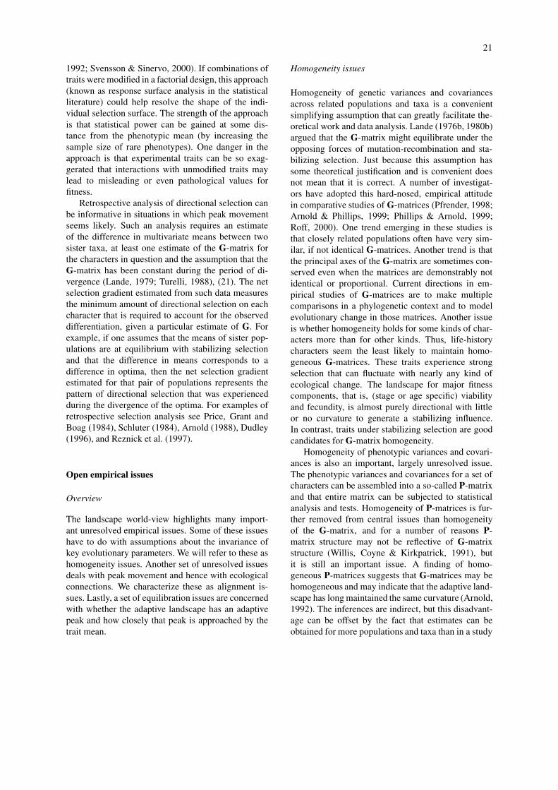
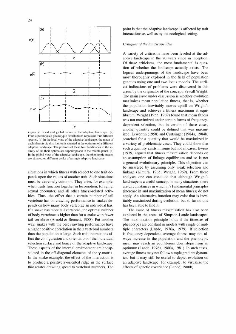
Even here we should not forget the distinctionbetween the individual selection surface and the ad-aptive landscape. Because of the smoothing effect ofthe trait distribution, the adaptive landscape can besmooth, even if the individual selection function isrugged and has multiple peaks (Figure 8). For manykinds of phenotypic characters, however, the land-scape beyond the limits of current variation in the pop-ulation is purely imaginary. For such characters it maybe gratuitous to assume that distant peaks exist. Theglobal view will often – perhaps always – be plaguedwith other serious limitations. The landscape for par-ticular species is bound to change through time, forexample. If we use a single landscape to predict the dy-namics of multiple species, we cannot account for thepossibility that different species may simultaneouslyexperience different changes in elevation at the samepoint in trait space. By forcing all populations andspecies to experience the same fitness at equivalentpoints in trait-space, the global view can seriously dis-tort reality. In contrast, the local perspective does notassume that all species reside on the same landscape.This perspective is also more in line with mathematicalcharacterizations of the adaptive landscape, which aretypically restricted to features near a particular phen-otypic mean. We can visualize multiple species, whileretaining an accurate view of each, by superimposingtheir adaptive landscapes (e.g., Schluter, 2000, Fig-ure 5.5). The distinction between the two perspectivescan be clearly seen in the case of an adaptive radi-ation in which descendant species occupy differentadaptive peaks. In the global view the landscape isnecessarily complex with mutliple peaks (Figure 9(c)).In the local view each species might have continuouslyexperienced a very simple local topography as it fol-lowed a moving peak. At a particular point in time,the superimposed landscapes for the different specieswould depict the sites of the different peaks in traitspace (Figure 9(b)). In other words, the fact that aclade shows diverse phenotypes (Figure 9a) does notforce us to adopt the global perspective.

Trait interactions provide another reason to viewthe landscape as a local phenomenon rather than as anecological reality that exists separately from the organ-ism and its population. By trait interactions we mean

24

Figure 9. Local and global views of the adaptive landscape. (a)Four superimposed phenotypic distributions represent four differentspecies. (b) In the local view of the adaptive landscape, the mean ofeach phenotypic distribution is situated at the optimum of a differentadaptive landscape. The portions of these four landscapes in the vi-cinity of the their optima are superimposed in the middle panel. (c)In the global view of the adaptive landscape, the phenotypic meansare situated on different peaks of a single adaptive landscape.

situations in which fitness with respect to one trait de-pends upon the values of another trait. Such situationsmust be extremely common. They arise, for example,when traits function together in locomotion, foraging,sexual encounter, and all other fitness-related activ-ities. Thus, the effect that a certain number of tailvertebrae has on crawling performance in snakes de-pends on how many body vertebrae an individual has.If a snake has more tail vertebrae, the optimal numberof body vertebrae is higher than for a snake with fewertail vertebrae (Arnold & Bennett, 1988). Put anotherway, snakes with the best crawling performance havea higher positive correlation in their vertebral numbersthan the population at large. Such trait interactions af-fect the configuration and orientation of the individualselection surface and hence of the adaptive landscape.These aspects of the internal environment are encap-sulated in the off-diagonal elements of the γγγ-matrix.In the snake example, the effect of the interaction isto produce a positively-oriented ridge in the surfacethat relates crawling speed to vertebral numbers. The

point is that the adaptive landscape is affected by traitinteractions as well as by the ecological setting.

Critiques of the landscape idea

A variety of criticisms have been leveled at the ad-aptive landscape in the 70 years since in inception.Of these criticisms, the most fundamental is ques-tion of whether the landscape actually exists. Thelogical underpinnings of the landscape have beenmost thoroughly explored in the field of populationgenetics using one and two locus models. The earli-est indications of problems were discovered in thisarena by the originator of the concept, Sewall Wright.The main issue under discussion is whether evolutionmaximizes mean population fitness, that is, whetherthe population inevitably moves uphill on Wright’slandscape and achieves a fitness maximum at equi-librium. Wright (1955, 1969) found that mean fitnesswas not maximized under certain forms of frequency-dependent selection, but in certain of these cases,another quantity could be defined that was maxim-ized. Lewontin (1958) and Curtsinger (1984a, 1984b)searched for a quantity that would be maximized ina variety of problematic cases. They could show thatsuch a quantity exists in some but not all cases. Ewens(1979) argued that fitness maximization depends onan assumption of linkage equilibrium and so is nota general evolutionary principle. This objection canbe answered by assuming only weak selection andlinkage (Kimura, 1965; Wright, 1969). From theseanalyses one can conclude that although Wright’slandscape is a useful concept in many situations, thereare circumstances in which it’s fundamental principles(increase in and maximization of mean fitness) do notapply. An alternative function may exist that is inev-itably maximized during evolution, but so far no onehas been able to find it.

The issue of fitness maximization has also beenexplored in the arena of Simpson-Lande landscapes.The maximization principle holds if the fitnesses ofphenotypes are constant in models with single or mul-tiple characters (Lande, 1976a, 1979). If selectionis frequency-dependent, average fitness may not al-ways increase in the population and the phenotypicmean may reach an equilibrium downslope from anoptimum (Lande, 1976a, 1980a, 1981). In such cases,average fitness may not follow simple gradient dynam-ics, but it may still be useful to depict evolution onan adaptive landscape, for example, to visualize theeffects of genetic covariance (Lande, 1980b).

25

Provine (1986) has criticized both Wright andSimpson–Lande landscapes, but on different grounds.Provine’s main complaint with Wright’s landscape isthat it is often confused with an individual selectionsurface in which the axes are particular genotypiccombinations (Provine, 1986, pp. 310–311). As Prov-ine points out, such an individual selection surfaceis not a continuous function and so it cannot be thesurface portrayed in Wright’s (1932) diagrams. Withregard to Wright’s landscape (mean fitness as a func-tion of gene frequency), Provine has no substantivecriticism. Turning to the Simpson–Lande landscape,Provine’s main objection is that the evolutionary dy-namics of the phenotypic mean are not formally re-lated to an underlying theory of change in gene fre-quencies. A tractable theory for phenotypic evolutionexplicitly rooted in equations for genetic change atmultiple loci is indeed a goal that has eluded theoreti-cians. The considerable progress that has been madein developing a useful evolutionary theory of phen-otypes (Lande, 1988) was achieved by purposefullydisconnecting that theory from population geneticsand hence from its failure to achieve a polygenic ex-tension. Whether one views this disconnection as anAchilles’ heal or an enabling tactic, depends on one’soutlook and priorities.

The Wrightian landscape is also at the center ofa controversy over Wright’s shifting balance theory,but the issues of contention loose their force whenapplied to the Simpson–Lande landscape. The mainissues of contention is whether populations becometrapped on a suboptimal peaks and then overcome thiscondition through the joint agency of drift and in-terdemic selection (Whitlock & Phillips, 2000). Thetrapped situation arises on Wrightian landscapes be-cause epistasis in fitness makes the landscape rugged(Whitlock et al., 1995). It is by no means clear thatepistasis in fitness will play a comparable role onthe Simpson–Lande landscape. In a highly polygenicworld, the landscape of phenotypic traits is likely tobe smooth. The prospect of becoming trapped is alsoexacerbated by the assumption that the landscape isconstant through time. If the landscape ripples as it’speak(s) move about, the population mean may workit’s way to the highest peak, even in the absence ofgenetic drift and interdemic selection.

Gould (1997) is dismayed by Dawkin’s (1996)Mount Improbable – a verbal portrayal of theSimpson–Lande landscape – because of what it leavesout. Gould prefers Lewontin’s metaphor of an envir-onmental trampoline; “since organisms help to create

their own environment, adaptive peaks are built by in-teraction and undergo complex shifts as populationsmove in morphospace”. Gould is disappointed becauseDawkin’s and Simpson’s landscapes leave out interac-tion between the organism and its environment, levelsof selection, and other complexities that add richnessto the discipline of evolutionary biology. Likewise,Eldredge and Cracraft (1980) and Eldredge (1999) ob-ject to the landscape concept because it leaves outselection at and above the level of species. None ofthese objections challenge the reality that we mustapproach the modeling of evolutionary processes indeliberate steps. The important point overlooked by allof the critiques just cited, as well as Dawkins (1996),is that the landscape concept is more than a metaphor.The landscape is a portrayal of a set of equations, nota bald invention. Those equations represent a growingset of models that capture an increasingly wider rangeof evolutionary possibilities. We may wish for mod-els (and metaphors) that capture all possibilities now,but in the meantime the most tangible way to progressconceptually is to test and extend the models that wehave.

What makes the adaptive landscape stable?

Under the landscape view of macroevolution the sta-bility of the adaptive landscape seems an inescapablefact. The Bauplans that are often characteristic ofgenera and higher taxa can be understood as manifest-ations of a stable landscape. The cause of long-termstability of the landscape remains, however, an incom-pletely solved problem. Williams (1992) refers to it asa ‘desperation hypothesis’. The problem of stabilityis lessened if we remember that the adaptive land-scape is not just an environmental phenomenon. Tosay that ‘the landscape is stable’ is not to say that ‘theenvironment is stable’. Organisms interact with theirenvironment and some kinds of interactions can pro-duce stability. Habitat selection (Partridge, 1978), forexample, is a powerful behavioral mechanism than cancompensate for environmental change and hence pro-mote landscape stability. Trait interaction is anotherpotential cause of stability. Traits that work togetherproduce ridges, saddles and other topographic featuresof the adaptive landscape. It seems plausible that suchfeatures, arising from trait interactions, lend stabil-ity to the landscape. Nevertheless, landscape stabilityis an issue that needs more theoretical and empiricalattention.

26

The theory of G-matrix evolution

The adaptive landscape provides the theoretical basisfor a connection between microevolution and macroe-volution, but to understand fully the flux of the land-scape and the evolutionary response of a population toa changing landscape, we need to understand the ge-netic underpinnings of the multivariate phenotype. Asnoted above, important aspects of the genetics of themultivariate phenotype can be described statisticallyusing the G-matrix. While most applications of the G-matrix assume that it remains relatively constant overevolutionary time, such an assumption may not alwaysbe valid. Unfortunately, the evolutionary dynamics ofthe G-matrix are not well understood. Despite morethan two decades of effort, a dynamic analytical the-ory for the evolution of the G-matrix has not beenproduced, because the mathematical challenges haveso far proven insurmountable. The problem has re-mained intractable because G-matrix stability dependson numerous factors, such as the number of loci affect-ing traits, the distribution of allelic effects at the loci,and the number of alleles per locus (Barton & Turelli,1987; Turelli, 1988). One conclusion from existingmodels of the G-matrix is that analytical theory cannotguarantee G-matrix stability (Shaw et al., 1995), butthe problem is so complex that existing theory can-not adequately describe the dynamics of the G-matrixover relevant periods of evolutionary time. Taken to-gether, empirical and theoretical results indicate thatthe G-matrix may or may not be stable over multiplegenerations, leaving the question of G-matrix stabilityan unresolved issue. Future theoretical work involvingboth simulations and analytical models, coupled withcareful empirical studies, may shed additional light onthis important topic.

Summary

Is the ‘modern synthesis’ incomplete? Eldredge andCracraft (1980) argue that microevolutionary pro-cesses cannot logically be extrapolated to explainmacroevolutionary pattern. This argument seems toevaporate with the demonstration that among-taxapatterns of trait covariance can be predicted frommodels of microevolutionary process. Furthermore,the predictions can be compared against null modelson a phylogeny. So long as that phylogeny includeshigher taxa (e.g., genera) as well as populations andspecies, the extrapolation seems logically complete.

Turning to the other main complaint – that importantpattern-producing processes operate above the level ofpopulations – accommodation within the frameworkof adaptive landscapes seems possible. In Simpson’s(1944) visualization of adaptive zones, for example,lineage-specific extinction is diagrammed and linkedto trait values. Continued construction of Simpson’sbridge, rather than demolition, may be the best pathforward.

Our review exonerates Simpson’s vision of a land-scape and suggests empirical and conceptual bridgesbetween the often separate endeavors of studyingmicro- and macroevolution. Models of microevolu-tionary process that make predictions about mac-roevolutionary pattern provide the bridge betweenthese endeavors. The key features of microevolution-ary process include quantitative inheritance (geneticvariances and covariances), effective population size,and configuration of the adaptive landscape (espe-cially peak position and local curvature). Analysesof phenotypic variation within populations can char-acterize both key features of inheritance and localfeatures of the landscape. Models that predict pat-tern from ecological processes are still poorly de-veloped. In particular, the elusive concept of ecolo-gical opportunity deserves more theoretical and em-pirical attention. Thus, although the first generation ofmodels provides many insights, much remains to bediscovered.

Acknowledgements

We are grateful to Thomas Hansen, Andrew Hendry,Russell Lande, Emilia Martins, and two anonymousreviewers for helpful comments on the manuscript.This work was supported by a NSF research grant toS.J. Arnold and M.E. Pfrender and a NIH postdoctoralfellowship to A.G. Jones.

Appendix

The results that follow depend on a series of assump-tions (Lande 1976a, 1979). The phenotypic distribu-tion of traits, p(z), is assumed to be (multivariate)normal, at least on some scale of measurement. Thedistribution of the breeding (additive genetic) valuesfor the traits is assumed to be (multivariate) nor-mal. This assumption of normally distributed breedingvalues does not necessarily imply that a very large

27

number of genes affect each trait. The assumption doesrequire that more than a few genes affect each trait(so that the central limit theorem applies), and thatno one gene explains the majority of genetic variance.Equations for the response of the phenotypic mean,z, to selection allow any form for the individual fit-ness function (selection surface), W(z), unless somespecial function is mentioned. Simple extrapolation ofthe selection response across more than one generationrequires that phenotypic and additive genetic variancesand covariances remain constant.

Matrices and vectors are shown in boldface. Allmatrices have n rows and n columns, where n is thenumber of traits. All vectors are column vectors withn elements. The superscript T denotes transpose. Thesuperscript −1 denotes matrix inverse. For a brief re-view of matrix operations in the context of multivariateinheritance and selection see Arnold (1994).

(1) If selection acts on a single character, thechange in the mean of that character, before selection,from one generation to the next is

�z = Gβ,

where G is the additive genetic variance of the charac-ter, and β is the directional selection gradient (Lande,1976a, p. 317). This gradient, the slope of the adaptivelandscape evaluated at the trait mean, is defined as

β = ∂ ln W

∂z.

(2) The change in the natural log of average fit-ness in response to selection is approximately equalto generalized genetic distance. Because this distanceis equal to or greater than zero, we can conclude thatthe effect of selection is to increase average fitness orleave it unchanged,

� ln W ≈ �zT G−1�z ≥ 0

(Lande, 1979, p. 406).(3) The change in the multivariate mean, before

selection, from one generation to the next is

�z = Gβββ,

where G is the additive genetic variance–covariancematrix, and βββ is a vector of directional selectiongradients,

βββ =

β1β2...

βn

,

whose n elements, corresponding to the n characters,are

βi = ∂ ln W

∂zi

(Lande, 1979, p. 406).(4) The curvature of the adaptive landscape in char-

acter dimensions zi and zj , evaluated at the trait mean,is

γij − βiβj = ∂2 ln W

∂zi∂zj

(Lande, 1979, p. 406; Phillips and Arnold, 1989,p. 1214), where γij is an element in the γγγ-matrix. Inthe two character case, the γγγ-matrix is

γγγ =[γ11 γ12γ12 γ22

],

where γ11 and γ22 describe curvature (negative ifcurvature is downward, positive if curvature is up-ward) in trait dimensions z1 and z2, respectively, andγ12 describes the orientation of the surface (positive ifthe surface tilts upward, negative if it tilts downward).

(5) The G-matrix can be expressed in terms of itsprincipal components (eigenvectors) and eigenvalues,

G = M���MT,

where M is an orthogonal matrix whose columns arethe principal components of G, and ��� is a matrixwith the eigenvalues of G on its diagonal and zeroselsewhere (Flury, 1988, Chap. 2). Abundant geneticvariation in a particular direction in trait-space (prin-cipal component) is equivalent to a large eigenvaluefor the corresponding principal component.

(6) For multiple traits, the among-populationvariance–covariance matrix for trait means after t

generations is

COV[z] =(

t

Ne

)G,

where Ne is effective population size and G is the timeaverage of G (Lande, 1979, pp. 408–409).

(7) For multiple traits after t generations,

COV[z] = tGCOV[βββ]G,

where COV[βββ] is the among-population variance–covariance matrix for βββ, the directional selectiongradient, and

COV[βββ] = P−1sP−1,

where P is the variance–covariance matrix for thetraits before selection, and s is the column vector of

28

directional selection differentials (Felsenstein, 1988,pp. 451–452; Zeng, 1988, p. 370). For a single trait,the among-population variance in trait mean after t

generations is

VAR(z) = t (G2/P 2)VAR(s),

where G is additive genetic variance, P is phen-otypic variance before selection and Var(s) is theamong-population variance in the directional selectiondifferential for the trait.

(8) For multiple traits,

COV[z] = t[G/Ne + GCOV[βββ]G](Hansen & Martins, 1996, p. 1409).

(9) For multiple traits, the restraining force is

G[P − γγγ−1

]≈ −Gγγγ,

assuming weak selection (Hansen & Martins, 1996,p. 1410). Note that if selection is weak, so that β ≈ 0and ωωω P, where ωωω is a matrix whose elementsdescribe a Gaussian individual selection surface (ele-ments of ωωω analogous to variances and covariances),then

ωωω ≈ −γγγ−1

(Lande, 1979, pp. 406–407). Hansen and Martin(1996) use W to represent ωωω−1. In the univariate case,ω2 is sometimes used to represent the ‘variance’ ofa Gaussian selection surface (e.g., Lande, 1976), inwhich case ω2 ≈ −1/γ .

(10) For multiple traits after t generations,

COV[z] = Q(t)VQT(t),

where

Q(t) = exp(tGγγγ)

and

V = −(2Neγγγ)−1

(Hansen & Martins 1996, p. 1410). For a single traitafter t generations,

Var(z) = −(2Neγ )−1 exp(2tGγ ).

(11) The expected time until the trait mean shiftsto the second adaptive peak is

T ∝ (WpWv)2Ne ,

where Wp represents the height of the original peakand Wv represents the height of the valley between thetwo peaks (Lande, 1986, p. 345).

(12) For a single trait, the expected change in thetrait mean is

�z = −Gγd,

where d is the distance of the trait mean from theoptimum (Lande & Shannon, 1996, p. 435).

(13) For multiple traits in large populations after tgenerations,

COV[zzz] = Q(t)COV[θθθ]QT (t),

where COV[θθθ ] is the among-population variance–covariance matrix for the optima of the adaptive land-scapes (Hansen & Martins, 1996, p. 1411). For asingle trait after t generations,

Var(z) = Var(θ) exp(2tGγ ),

where Var(θ ) is the among-population variance in theoptima of the adaptive landscapes.

(14) Let the individual selection surface be a Gaus-sian surface with optimum θ ,

W(z) = exp[− 1

2 (z − θθθ)Tωωω−1(z − θθθ)].

Suppose the optimum of the surface moves as a nor-mally distributed random variable with mean 0 and avariance–covariance matrix that is proportional to ωωω.Then, if selection is weak, so that βββ ≈ 0 and ωωω P,

COV(θθθ) = kωωω = −kγγγ−1,

where k is a constant of proportionality (a scalar).Then, using (13), the among-population variance–covariance matrix for trait means after t generationsis

COV[z] = Q(t)(kωωω)QT(t) ≈ Q(t)(−kγγγ−1)QT(t).

For a single trait after t generations,

Var(z) = (kω) exp(−2tG/ω)

≈ (−k/γ ) exp(2tGγ ).

(15) The evolutionary load caused by the deviationof the trait mean from its optimum after t generationsis

(γ /2)E[z(t) − θ(t)]2,

where the second term represents the expected valueof the squared deviation of the trait mean from its op-timum after t generations (Lande & Shannon, 1996,p. 435).

(16) The directional selection differential is thechange in trait mean within a generation arising fromdirectional selection

s = �z∗z∗z∗ − zzz� = Pβββ,

29

where z∗ is the trait mean after selection and z is thetrait mean before selection (Lande & Arnold, 1983,p. 1213). The shift in the mean of trait z1 due todirectional selection is

s1 = (z∗1 − z1) = P11β1 + P12β2 + · · · + P1nβn,

where P11β1 is the portion of the shift due to selectionon trait z1, P12β2 is the portion of the shift due toselection on trait z2, and P1nβn is the portion of theshift due to selection on trait zn.

(17) The nonlinear selection differential is thechange in trait variance and covariance within a gen-eration arising from nonlinear selection

C = P∗ − P + ssT = PγγγP,

where P∗ is the trait variance–covariance matrix afterselection (Lande & Arnold, 1983, p. 1216). In the caseof two traits under selection, the change in the varianceof trait z1 due to nonlinear selection is

C11 = P ∗11 − P11 + s2

= P 211γ11 + 2P11P12γ12 + P 2

12γ22,

where the s12 term corrects for the decrease in vari-

ance arising from directional selection. The P112γ11

term describes the change in variance due to nonlinearselection on trait z1 (γ11 is negative in the case of sta-bilizing selection and positive in the case of disruptiveselection). The P11P12γ12 term describes the changein variance of trait z1 due to correlational selection ontraits z1 and z2. The P12

2γ22 term describes the changein variance of trait z1 due to nonlinear selection on traitz2.

(18) The individual selection surface can often beapproximated by a quadratic surface, which in the caseof two traits, is

W(z) = α + β1z1 + β2z2 + 12γ11z

21

+ 12γ22z

22 + γ12z1z2,

where α is a constant, z1 and z2 are the trait valuesfor the two traits (standardized so that their means= 0), β1 and β2 are the directional selection gradientsfor the two traits, γ11 and γ22 are the nonlinear se-lection gradients describing stabilizing (or disruptive)selection, and γ12 is the nonlinear selection gradientdescribing correlational selection. This quadratic sur-face can be estimated from data using the quadraticregression model

w = α + β1z1 + β2z2 + 12γ11z

21 + 1

2γ22z22

+γ12z1z2 + ε,

where w is relative fitness (standardized so that itsmean = 1), α is a constant, and ε is an error term(Lande & Arnold, 1983, p. 1217).

(19) The directional selection gradient is theslope of the individual selection surface, ∂W(z)/∂z,weighted by the phenotypic trait distribution beforeselection, p(z);

β =∫

p(z)∂W(z)∂z

dz

(Lande & Arnold, 1983, p. 1213).(20) The nonlinear selection gradient is the

curvature of the individual selection surface, ∂2W(z)/∂2z, weighted by p(z);

γ =∫

p(z)∂2W(z)∂2z

dz

(Lande & Arnold, 1983, p. 1216).(21) The net selection gradient corresponding to

the phenotypic divergence of two sister taxa is thesum of over generations of the directional selectiongradients, βt , that have acted during the period of di-vergence. If G remains constant during the period ofdivergence, the net selection gradient can be estimatedby the formula,

βnet = G−1[zzza − zzzb],where zzza and zzzb are the trait means of two sister taxa(Lande, 1979, p. 407). If G varies during the periodof divergence, the net divergence in means is a func-tion of the covariance between G and βββ, COV(Gt , βββt ),as well as the time average of G and the sum of βββt

(Turelli, 1988). Although Turelli (1988) argued thatCOV(Gt , βββt ) might be large, it is not clear that this isso. Selection in generation t affects G in generationt + 1. Thus, we might expect a nonzero COV(Gt+1,βββt ), if βββt varies. Nonzero COV(Gt , βββt ) would dependon serial autocorrelation in βββt . This autocorrelationobviously depends on how the adaptive landscape var-ies through time, which is an unresolved empiricalissue.

References

Arnold, S.J., 1988. Quantitative genetics and selection in naturalpopulations: microevolution of vertebral numbers in the gartersnake, Thamnophis elegans, pp. 619–636 in Proc. 2nd Intern.Conf. Quantitative Genetics, edited by B.S. Weir, E.J. Eisen,M.M. Goodman & G. Namkoong. Sinauer, Sunderland, M.A.

Arnold, S.J., 1992. Constraints on phenotypic evolution. Am. Nat.140: S85–S107.

30

Arnold, S.J., 1994. Multivariate inheritance and evolution: a reviewof the concepts, pp. 17–48 in Quantitative Genetic Studies ofthe Evolution of Behavior, edited by C.R.P. Boake. University ofChicago Press, Chicago.

Arnold, S.J. & A.F. Bennett, 1988. Behavioral variation in nat-ural populations. V. Morphological correlates of locomotionin the garter snake Thamnophis radix. Biol. J. Linn. Soc. 34:175–190.

Arnold, S.J. & P.C. Phillips, 1999. Hierarchical comparison ofgenetic variance–covariance matrices. II. Coastal-inland diver-gence in the garter snake, Thamnophis elegans. Evolution 53:1516–1527.

Badyaev, A.V. & G.E. Hill, 2000. The evolution of sexual dimorph-ism in the house finch. I. Population divergence on morpholo-gical covariance structure. Evolution 54: 1784–1794.

Barton, N.H. & M. Turelli, 1987. Adaptive landscapes, genetic dis-tance and the evolution of quantitative characters. Genet. Res.49: 157–173.

Brodie, E.D. III, 1992. Correlational selection for color pattern andantipredator behavior in the garter snake Thamnophis ordinoides.Evolution 47: 1284–1298.

Brodie, E.D. III, A.J. Moore & F.J. Janzen, 1995. Visualizing andquantifying natural selection. Trends Ecol. Evol. 10: 313–318.

Brown, J.S. & T.L. Vincent, 1992. Organization of predator-preycommunities as an evolutionary game. Evolution 46: 1269–1283.

Bull, J.J., 1987. Evolution of phenotypic variance. Evolution 41:303–315.

Charlesworth, B., 1993a. The evolution of sex and recombination ina varying environment. J. Hered. 84: 345–350.

Charlesworth, B., 1993b. Directional selection and the evolution ofsex and recombination. Genet. Res. 61: 205–224.

Charlesworth, B., R. Lande & M. Slatkin, 1982. A neo-Darwiniancommentary on macroevolution. Evolution 36: 474–498.

Cheverud, J.M., 1984. Quantitative genetics and developmental con-straints on evolution by selection. J. Theor. Biol. 110: 155–171.

Curtsinger, J.W., 1984a., Evolutionary landscapes for complexselection. Evolution 38: 359–367.

Curtsinger, J.W., 1984b. Evolutionary principles for polynomialmodels of frequency-dependent selection. Proc. Natl. Acad. Sci.81: 2840–2842.

Dawkins, R., 1996. Climbing Mount Improbable. W.W. Norton,New York.

Dudley, S.A., 1996. The response to differing selection on plantphysiological traits: evidence for local adaptation. Evolution 50:103–110.

Eldredge, N., 1999. The Pattern of Evolution. W.H. Freeman andCo., New York.

Eldredge, N. & J. Cracraft, 1980. Phylogenetic Patterns and theEvolutionary Process. Columbia University Press, New York,N.Y.

Emerson, S.B. & S.J. Arnold, 1989. Intra- and interspecific rela-tionships between morphology, performance, and fitness, pp.295–314 in Complex Organismal Functions: Integration andEvolution, edited by D.B. Wake & G. Roth. Wiley, Chichester,U.K.

Endler, J.A., 1986. Natural Selection in the Wild. Princeton Univer-sity Press, Princeton, N.J.

Ewens, W.J., 1979. Mathematical Population Genetics. Springer-Verlag, New York.

Feder, J.F., 1998. The apple maggot fly, Rhagoletis pomonella: fliesin the face of conventional wisdom, pp. 130–144 in EndlessForms: Species and Speciation, edited by D.J. Howard & S.H.Berlocher. Oxford University Press, New York.

Felsenstein, J., 1973. Maximum likelihood estimation of evolution-ary trees from continuous characters. Am. J. Hum. Genet. 25:471–492.

Felsenstein, J., 1979. Excursions along the interface between dis-ruptive and stabilizing selection. Genetics 93: 773–795.

Felsenstein, J., 1985. Phylogenies and the comparative method. Am.Nat. 125: 1–15.

Felsenstein, J., 1988. Phylogenies and quantitative characters. Ann.Rev. Ecol. Syst. 19: 445–471.

Flury, B., 1988. Common Principal Components and Related Mul-tivariate Models. Wiley, New York, N.Y.

Garcia-Ramos, G. & M. Kirkpatrick, 1997. Genetic models of ad-aptation and gene flow in peripheral populations. Evolution 51:21–28.

Gavrilets, S., 1997. Evolution and speciation on holey adaptivelandscapes. Trends Ecol. Evol. 12: 307–312.

Gould, S.J., 1997. Self-help for a hedgehog stuck on a molehill.Evolution 51: 1020–1023.

Gould, S.J. & N. Eldredge, 1977. Punctuated equilibria: the tempoand mode of evolution reconsidered. Paleobiol. 3: 115–151.

Hansen, T.F. & E.P. Martins, 1996. Translating between microevolu-tionary process and macroevolutionary patterns: the correlationstructure of interspecific data. Evolution 50: 1404–1417.

Hansen, T.F., 1997. Stabilizing selection and the comparativeanalysis of adaptation. Evolution 51: 1341–1351.

Hendry, A.P. & M.T. Kinnison, 1999. The pace of modern life:measuring rates of microevolution. Evolution 53: 1637–1653.

Hendry, A.P., J.K. Wenburg, P. Bentzen, E. C. Volk & T. P. Quinn,2000. Rapid evolution of reproductive isolation in the wild:evidence from introduced salmon. Science 290: 516–518.

Hendry, A.P., T. Day & E. B. Taylor, 2001. Population mixing andthe adaptive divergence of quantitative characters in discrete pop-ulations: a theoretical framework for empirical tests. Evolution55: 459–466.

Janzen, F.J. & H.S. Stern, 1998. Logistic regression for empiricalstudies of multivariate selection. Evolution 52: 1564–1571.

Karn, M.L. & L.S. Penrose, 1951. Birth weight and gestation timein relation to maternal age, parity, and infant survival. Ann.Eugenics 16: 147–164.

Kimura, M., 1965. Attainment of quasi-linkage equilibrium whengene frequencies are changing by natural selection. Genetics 52:875–890.

Kingsolver, J.G., H.E. Hoekstra, J.M. Hoeskstra, D. Berrigan, S.N.Vignieri, C.E. Hill, A. Hoang, P. Gilbert & P. Beerli, 2001. Thestrength of phenotypic selection in natural populations. Am. Nat.157: 245–261.

Kirkpatrick, M., 1982. Quantum evolution and punctuated equilib-rium in continuous genetic characters. Am. Nat. 119: 833–848.

Kurtén, B., 1959. Rates of evolution in fossil mammals. Cold SpringHarbor Symp. Quant. Biol. 24: 205–215.

Lande, R., 1976a. Natural selection and random genetic drift inphenotypic evolution. Evolution 30: 314–334.

Lande, R., 1976b. The maintenance of genetic variability by muta-tion in a polygenic character with linked loci. Genet. Res. 26:221–235.

Lande, R., 1979. Quantitative genetic analysis of multivariateevolution, applied to brain-body size allometry. Evolution 33:402–416.

Lande, R., 1980a. Microevolution in relation to macroevolution.Paleobiol. 6: 233–238.

Lande, R., 1980b. Sexual dimorphism, sexual selection, and adapt-ation in polygenic characters. Evolution 34: 292–305.

Lande, R., 1980c. The genetic covariance between charactersmaintained by pleiotropic mutation. Genetics 94: 203–215.

31

Lande, R., 1981. The minimum number of genes contributing toquantitative variation between and within populations. Genetics99: 541–553.

Lande, R., 1986. The dynamics of peak shifts and the pattern ofmorphological evolution. Paleobiol. 12: 343–354.

Lande, R., 1988. Genetics and demography in biological conserva-tion. Science 241: 1455–1460.

Lande, R. & S.J. Arnold, 1983. The measurement of selection oncorrelated characters. Evolution 37: 1210–1226.

Lande, R. & S. Shannon, 1996. The role of genetic variation in ad-aptation and population persistence in a changing environment.Evolution 50: 434–437.

Lewontin, R.C., 1958. A general method for investigating theequilibrium of gene frequencies in a population. Genetics 43:419–434.

Lynch, M., 1990. The rate of morphological evolution in mammalsfrom the standpoint of neutral expectation. Am. Nat. 136: 727–741.

Lynch, M. & R. Lande, 1993. Evolution and extinction in responseto environmental change, pp. 234–250 in Biotic Interactions andGlobal Change, edited by P. Kareiva, J.G. Kingsolver & R.B.Huey. Sinauer, Sunderland, MA.

Martins, E.P. & T.F. Hansen, 1996. A microevolutionary linkbetween phylogenies and comparative data, pp. 273–288 in NewUses of New Phylogenies, edited by P.H. Harvey, A.J. LeighBrown, J. Maynard Smith & S. Nee. Oxford University Press,Oxford, U.K.

Mather, K., 1941. Variation and selection of polygenic characters. J.Genetics 41: 159–193.

Partridge, L., 1978. Habitat selection, pp. 351–376 in Behavi-oral Ecology, edited by J.R. Krebs & N.B. Davies. BlackwellScientific, Oxford, England.

Pfrender, M., 1998. Evolutionary dynamics of molecular and quant-itative genetic variation in ephemeral pond populations of Daph-nia pulex. Thesis Dissertation, University of Oregon, Eugene,Oregon.

Phillips, P.C. & S.J. Arnold, 1989. Visualizing multivariate selec-tion. Evolution 43: 1209–1222.

Phillips, P.C. & S.J. Arnold, 1999. Hierarchical comparison of ge-netic variance–covariance matrices. I. Using the Flury hierarchy.Evolution 53: 1506–1515.

Phillips, P.C., M.C. Whitlock & K. Fowler, 2001. Inbreedingchanges the shape of the genetic covariance matrix in Drosophilamelanogaster. Genetics 158: 1137–1145.

Price, T.D., P.R. Grant & P.T. Boag, 1984. Genetic changes inthe morphological differentiation of Darwin’s ground finches,pp. 49–66 in Population Biology and Evolution, edited by KWohrmann & V. Loeschske. Springer-Verlag, Berlin.

Provine, W.B., 1986. Sewall Wright and Evolutionary Biology.University of Chicago Press, Chicago, I.L.

Rensch, B., 1959. Evolution Above the Species Level. Wiley, NewYork, N.Y.

Reznick, D.N. & C.K. Ghalambor, 2001. The population eco-logy of contemporary adaptations: what empirical studies revealabout the conditions that promote adaptive evolution. Genetica112-113: 183–198.

Reznick, D.N., F.H. Shaw, F.H. Rodd & R.G. Shaw, 1997. Evalu-ation of the rate of evolution in natural populations of guppies(Poecilia reticulata). Science 275: 1934–1937.

Rieseberg, L.H., M.A. Archer & R.K. Wayne, 1999. Transgressivesegregation, adaptation and speciation. Heredity 83: 363–372.

Rice, S.H., 1998. The evolution of canalization and the breakingof von Baer’s laws: modeling the evolution of development withepistasis. Evolution 52: 647–656.

Roff, D.A., 2000. The evolution of the G matrix: selection or drift?Heredity 84: 135–142.

Rundle, H.D. & M.C. Whitlock, 2001. A genetic interpretation ofecologically dependent isolation. Evolution 55: 198–201.

Schluter, D., 1984. Morphological and phylogenetic relationsamong the Darwin’s finches. Evolution 38: 921–930.

Schluter, D., 1988. Estimating the form of natural selection on aquantitative trait. Evolution 42: 849–861.

Schluter, D., 1996. Adaptive radiation along genetic lines of leastresistance. Evolution 50: 1766–1774.

Schluter, D. & D. Nychka, 1994. Exploring fitness surfaces. Am.Nat. 143: 597–616.

Schluter, D., 2000. The Ecology of Adaptive Radiation. OxfordUniversity Press, Oxford, England.

Schmalhausen, I.I., 1949. Factors of Evolution, The Theory ofStabilizing Selection. University of Chicago Press, Chicago,I.L.

Shaw, F.H., R.G. Shaw, G.S. Wilkinson & M.H. Turelli, 1995.Changes in genetic variances and covariances: G whiz! Evolution49: 1260–1267.

Simpson, G.G., 1944. Tempo and Mode in Evolution. ColumbiaUniversity Press, New York, N.Y.

Simpson, G.G., 1953. The Major Features of Evolution. ColumbiaUniversity Press, New York.

Sinervo, B., P. Doughty, R.B. Huey & K. Zamudio, 1992. Al-lometric engineering: a causal analysis of natural selection onoffspring size. Science 258: 1927–1930.

Slatkin, M. & R. Lande, 1976. Niche width in a fluctuatingenvironment – density independent model. Am. Nat. 110: 31–55.

Stanley, S.M., 1979. Macroevolution: Pattern and Process. W. H.Freeman and Co., San Francisco.

Steppan, S.J., 1997a. Phylogenetic analysis of phenotypic covari-ance structure. I. Contrasting results from matrix correlationand common principal component analyses. Evolution 51: 571–586.

Steppan, S.J., 1997b. Phylogenetic analysis of phenotypic covari-ance structure. II. Reconstructing matrix evolution. Evolution 51:587–594.

Svensson, E. & B. Sinervo, 2000. Experimental excursions onadaptive landscapes: density-dependent selection on egg size.Evolution 54: 1396–1403.

Thompson, J.N., 1998. Rapid evolution as an ecological process.Trends Ecol. Evol. 13: 329–332.

Turelli, M., 1988. Phenotypic evolution, constant covariances, andthe maintenance of additive variance. Evolution 42: 1342–1347.

Via, S., 1991. The genetic structure of host plant adaptation in aspatial patchwork: demographic variability among reciprocallytransplanted pea aphid clones. Evolution 45: 827–852.

Vrba, E.S., 1983. Macroevolutionary trends: new perspectives onthe roles of adaptation and incidental effect. Science 221: 387–389.

Waddington, C.H., 1957. The Strategy of the Genes. MacMillan,New York, N.Y.

Williams, G.C., 1992. Natural Selection: Domains, Levels, andChallenges. Oxford University Press, Oxford, U.K.

Willis, J.H., J.A. Coyne & M. Kirkpatrick, 1991. Can one predict theevolution of quantitative characters without genetics? Evolution45: 441–444.

Whitlock, M.C., 1995. Variance-induced peak shifts. Evolution 49:252–259.

Whitlock, M.C. & P. C. Phillips, 2000. The exquisite corpse: ashifting view of the shifting balance. Trends Ecol. Evol. 15:347–348.

32

Whitlock, M.C., P.C. Phillips, F.B.-G. Moore & S.J. Tonsor, 1995.Multiple fitness peaks and epistasis. Ann. Rev. Ecol. Syst. 26:601–629.

Wright, S., 1931. Evolution in Mendelian populations. Genetics 16:97–159.

Wright, S., 1932. The roles of mutation, inbreeding, crossbreeding,and selection in evolution. Proc. VI Inter. Congr. Genet. 1: 356–366.

Wright, S., 1940. The statistical consequences of Mendelian hered-ity in relation to speciation, pp. 161–183 in The New Systemat-ics, edited by J.S. Huxley. Clarendon Press, Oxford.

Wright, S., 1945. Tempo and mode in evolution: a critical review.Ecology 26: 415–419.

Wright, S., 1955. Classification of the factors of evolution. ColdSpring Harbor Symp. Quant. Biol. 20: 16–24.

Wright, S., 1968. Evolution and the Genetics of Populations, Vol.1. Genetic and Biometric Foundations. University of ChicagoPress, Chicago, I.L.

Wright, S., 1969. Evolution and the Genetics of Populations, Vol. 2.The Theory of Gene Frequencies. University of Chicago Press,Chicago, I.L.

Wright, S., 1982. Character change, speciation, and the higher taxa.Evolution 36: 427–443.

Zeng, Z.-B., 1988. Long-term correlated response, interpopu-lation covariance, and interspecific allometry. Evolution 42:363–374.