the adage gallery tour i: highlights - …adage.sourceforge.net/doc/highlights/highlights.pdf ·...

THE ADAGE GALLERY TOURI: HIGHLIGHTS

J. ALEX STARK

CONTENTS

1. Introduction . . . . . . . . . . . . . . . . . . . . . . . . . . . . . . . 22. Basic drawings . . . . . . . . . . . . . . . . . . . . . . . . . . . . . . 32.1. Basics: Geometrical elements . . . . . . . . . . . . . . . . . . . . . 32.2. Basics: Drawing construction . . . . . . . . . . . . . . . . . . . . 63. Connected nodes . . . . . . . . . . . . . . . . . . . . . . . . . . . . . 83.1. Connected nodes: Flow charts . . . . . . . . . . . . . . . . . . . . 83.2. Connected nodes: Nodal graphs . . . . . . . . . . . . . . . . . . 103.3. Connected nodes: Schematic diagrams . . . . . . . . . . . . . . 124. Representing reality . . . . . . . . . . . . . . . . . . . . . . . . . . 144.1. Representing reality: Drafting . . . . . . . . . . . . . . . . . . . 144.2. Representing reality: Architectural . . . . . . . . . . . . . . . . 165. Plotting and charting . . . . . . . . . . . . . . . . . . . . . . . . . 185.1. Plotting and charting: 2-D function plotting . . . . . . . . . . . 185.2. Plotting and charting: 2-D statistical plotting . . . . . . . . . . 205.3. Plotting and charting: Data charts and plots . . . . . . . . . . . 225.4. Plotting and charting: The virtual oscilloscope . . . . . . . . . 245.5. Plotting and charting: 3-D plotting . . . . . . . . . . . . . . . . 26

For further information email [email protected] .1

GALLERY TOUR HIGHLIGHTS 2

1. INTRODUCTION

This document is a work in progress.The aim of the Adage project is to develop a powerful, flexible and ex-

tensible drawing engine. This document is a pictorial survey of drawinggenres; it sets out the vision for the project by example.

The survey is designed to be representative of the forms of drawing tobe supported. The drawings are composed entirely of lines, points, filledareas, and text. They are grouped into categories, as follows.

Basic drawings: These drawings are simple and illustrate the basicoperation of the Adage system.

Connected nodes: Many drawings are composed of nodes that areconnected together. Nodes sometimes represent objects (nouns),and others processes or actions (verbs) with inputs and outputs.Connections indicate relationships, dependencies, sequences andtransfers (such as outputs to inputs).

Representing reality: Typically the most sophisticated type, these draw-ings are a literal representation of something real. This category in-clues engineering drawing and architecture.

Plotting and charting: A major category of drawing is the representa-tion of data. Often the aim is illustration with impact, rather thanprecise detail.

Note that many of these drawings would not be produced by Adage on itsown, but rather in combination with another program. For example, theplots of data would be produced by data analysis programs with Adage asthe output generator.


2. BASIC DRAWINGS

This section is devoted to a loose category of drawing: those that use thefundamental facilities of Adage. Some features of these include:

• The drawings are moderately simple compositions of lines, pointsand text, and of simple filled areas. Lines are either straight or basiccurves, such as circle arcs.

• Straightforward geometric construction is used. Examples are pointsof intersection of two lines, mid-points of lines, and perpendiculars.

• Angle-preserving transformations (scale, rotate, and translate) areemployed.

• Reasonable sophistication is required in text placement. In particu-lar, text can be placed with good controlled spacing next to a line orin a corner.

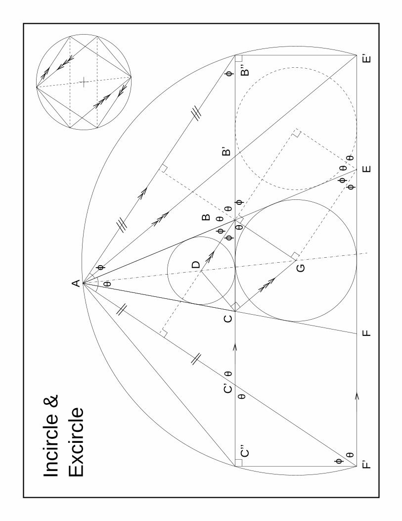
2.1. Basics: Geometrical elements. This sample is composition of straightlines, circles, circular arcs, and text. The layout of the entire (main) figureis defined by the three points of the triangle ABC. The position of the insetfigure would also need to be defined. The line styles, and drawn annota-tions would be specified. Ideally the locations of the text elements wouldbe defined in term of the lines and corners to which they are adjacent. Forinstance, the label ‘C’ might be placed in the corner of the lines C” to C andC to A.

The construction of the figure from the triangle ABC is quite simple. Theline BC is extended so that the length A to B’ equals A to C, and B to B”equals A to B. The points C’ and C” are similarly located. The incirclesand excircles are constructed, and the line through E and F is tangential tothe excircle and parallel to BC. The points E, F, E’ and F’ are found fromintersections. The angle CBD is ϕ, and θ is its complementary angle. Allother angles (and parallel-line relationships) follow by geometrical princi-ples. Proving that the lines C” to B” and B” to E’ are perpendicular is themost difficult step. One means is to use the inset figure. This is the quadri-lateral BDCG with a circle constructed on diameter DG. A copy is made ofthe quadrilateral, rotated through 180 degrees.

Drawing this figure in XFig required painstaking effort. The whole de-sign is based on Pythagorean triples, in order that every labelled point ex-cept for F be on a grid point. The line to F and some of the inset elementsare constructed using scaling and rotation. Once Adage is developed, itwill be fun to redraw the figure and experiment by moving point A aroundrelative to B and C.


Full-page figure on next page

FIGURE 1. The relative sizes of the incircle and excircle.Starting with the triangle ABC construct the incircle andan excircle. The rest of the drawing illustrates interrela-tionships between lines and points of intersection. Creationmethod: XFig, ps output. Category: .

C’

E’

F’

B’

A

θ

θ

θϕ

θ

θϕ

ϕ

ϕ

θϕ

Cθ

G

ϕ

BD

ϕθ

ϕθ

EF

B’’

C’’

Inci

rcle

&E

xcirc

le


2.2. Basics: Drawing construction. This figure illustrates some features ofthe Adage system for drawing. It complements the geometric constructionshown in the preceding section. In this case we consider a drawing ele-ment that might be used as a node in a connected drawing: a NAND gatefor electronic schematics. NAND gates can be used in slightly differentways (A in the figure), depending on the number of inputs. The underly-ing macro (B) is the same, and we have chosen a typical set of defining pa-rameters, namely the output point, the orientation angle and the gate-sizelength. These values (rounded rectangles) are inputs to the create NANDgate action (ordinary rectangle).

The process of creating such a macro might be elaborate, but Adage isdesigned so that this can be done in the interactive program. We createa standardized form of the gate (C). This might be done using a 4-pointpolyline, a 3-pt circular arc, and a circle. These would then be groupedas a set. In order to convert this into a drawing-element macro, we wouldspecify that the six points and the six numerical values are constants built into the macro rather than inputs. The general NAND gate is then (D) createdfrom the standardized NAND (an object) by applying resizing, rotation andtranslation transformations.

This framework of a standardized constant object transformed by pa-rameters is very common. Therefore templates are provided along with aninheritance mechanism to make this straightforward.


FIGURE 2. A NAND Gate. The electronic schematic NANDgate element (A), and a possible parameterisation (B), andimplementation (C and D). Creation method: XFig, ps out-put. Category: .

point

point

point

point

point

point

3−pt arc

2−pt circle

Gate−size

Orientation

NAND−output

A. Usage:

−0.4

0.4

−1.2 −0.6 −0.2

Exampleelement:NAND Gate

B. Macro:

Gate−size

NAND Gate

C. Standardized:

−0.6

0.4

−1.2

−0.4

−0.2

0.0

sequ

ence

polyline

set

Orientation

NAND−output

D. SRT Transformation:

Standardized NAND

NAND Gate

NAND

StandardizedSCALE TRANSLATEROTATE


3. CONNECTED NODES

A wide variety of drawings are in structure a set of nodes and connec-tions. Some examples are:

• Family trees, or genealogies; phylogenetic trees;• Software flow diagrams;• Software call graphs;• State diagrams;• Dependency graphs;• Hierarchies, reporting structures and organisation charts;• Electrical and electronic schematics;• Pneumatic and hydraulic schematics;• Communication network diagrams.

3.1. Connected nodes: Flow charts. This is an example of a system di-agram with internal function blocks, connections that carry signals, andlinks to external signals and devices. It is slightly more elaborate than asoftware flow chart in which the flow is typically sequential.


FIGURE 3. Controller System. Diagram of the controller of arobotic positioning system. Creation method: XFig, ps out-put. Category: .

EN

C0−7EN C8−14EN EN EN EN

C>R

C=R

C<R

R0−7R8−15

EN EN

C

C

8

A0

A1

R/NW

A0

A1

C=0

CRST

HLT

DRN

ERR

MCK

FRQ

LPOS

EHLT

HPOS

MSTP

17

DMUX3−8 line

Address

Act. pos.

decoder

MSByteAct. pos.LSByte

Status Commandregisterregister

14−bitDAC

VFO15−bit up/down counter

Comparator

Motor driverboard

Req. pos.MSByte

Req. pos.LSByte

logicCondition

MOTOR

Address BusR/NWData Bus

HaltHigh pos. Low pos.


3.2. Connected nodes: Nodal graphs. This is a detailed call graph. Incontrast with the controller example, which was edited in an interactivedrawing package, this was automatically generated by running a profileron a program, and then processing the results in a package for visualisinggraphs.

Note that in this case ‘graph’ has the specific meaning of nodes connected byedges.

This example also makes a distinction between interactive drawings andthe use of the Adage system as a library for generating output. It is impor-tant to remember that it is not an aim of the project to create such a drawingfrom scratch. The Adage system would render the drawing, but the task oflaying out the elements is separate.


FIGURE 4. Call Graph. The procedural call graph ofthe pnmace program. Numbered edges indicate calls thatwere made more than once. Creation method: gprof andGraphviz dot programs, ps output. Category: .

Process

GenGen34

InitAccIm

WIsError

36

SetForTerm

34

SetTables34

TermlyReport17

WMessage17

WindChk

Output

26

CallFilt

26BigGrayAccumulate

26

17

WPutImgRowFinish512

WPutImgRowStart

512

WErrorValue

WPutImgStart

WPutImgFinish

main

5

AllocClientData

WInit

Pnm_Init

CfgInit

ParseArgs

CfgAllocSeriesVectors

Pnm_ScanListfiles

CfgBeginToHeseries

CfgHeseriesToAddback

CFuncGen

Pnm_ReadImgArrays

CfgAddbackToEnd

AllocTables

DefaultTmpImg

AllocImgArrays

CfgFreeSeriesVectors

FreeImgArrays

FreeTables FreeClientData

Pnm_CloseFile

WMalloc

4

WDataAlloc

WWrapTell

WKeyMatch52

WOpenImage

CallocReallocFree

HeseriesVal17

HeseriesInit

PnmReadOneImg

WCalloc

SetTmpImg

2

2

WFree2

5

26

FiltWind26

FillTableForNotFilt26

WindTableFillAll26

FillTableForFilt

26

3

4

PNMACECall Graph


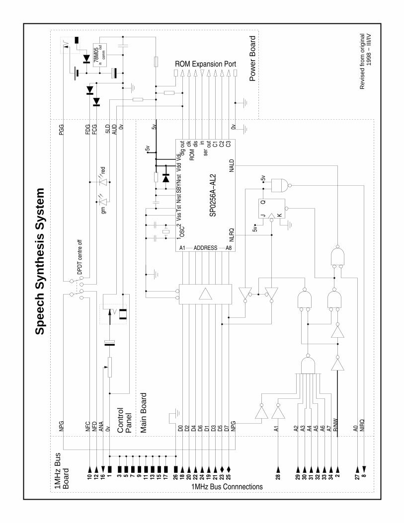
3.3. Connected nodes: Schematic diagrams. Circuit diagrams and schemat-ics have a richer variety of node types than other drawing of connectednodes. This example includes a representative range of digital and ana-logue components, both integrated and discrete.

The circuit comes from a system that the author designed and built inhigh school. (Desktop computers were only just beginning to be able tohandle the computational requirements of speech synthesis at that time.)The original was drawn by hand. Drawing in XFig was not much easier,adding the flexibility of rearranging elements, but making text placementtedious.


FIGURE 5. Speech Synthesis System. Circuit diagram of aspeech system. This comprised a speech synthesis IC, aninterface to the 1MHz bus of a BBC Microcomputer, powerregulation and audio analogue output. Creation method:XFig, ps output. Category: .

DPDT

cen

tre o

ff

SP02

56A−

AL2

78M

05

NLRQ

NALD

12

OSC

VssT

stNr

stVd

d

clkdi

g ou

tVd

iSB

YNrs

t

dis in out

C1 C2 C3

ROM ser

QJ K

A1 A8ADDRESS

grn

red

5v

com

mou

tin

5v5v

NPG

NFC

NFD

ANA

0v D0 D2 D4 D6 D1 D3 D5 D7 NPG

A1 A2 A3 A4 R/NW

A5 A6 A7 A0 NIRQ

1MHz Bus Connnections

PGG

FDG

FCG

AUD 0v

5LD 5v

ROM Expansion Port

0v

26 18 20 22 24 19 21 2523 28 29 30 31 32 33 34 2 27 81161210 3 5 7 9 11 13 15 17

1MH

z B

usB

oard

Pow

er B

oard

Con

trol

Pan

el

Mai

n B

oard

Rev

ised

from

orig

inal

1998

− II

I/IV

Sp

eech

Syn

thes

is S

yste

m


4. REPRESENTING REALITY

Whereas drawings of connected nodes depict logical and functional rela-tionships, and plots illustrate features of data and functions, the drawingsin this category are a literal representation of reality. Reality gets compli-cated, and so these drawings can be very intricate. We consider two subdi-visions. First there are representations of objects that are manufactured forfunctional or aesthetic purposes. Second, there are larger-scale drawings ofbuildings and land, urban plans, and maps.

4.1. Representing reality: Drafting. This is a simple engineering drawingin first angle projection of a plastic shelf pin. These are a version of pinsused in adjustable bookshelves. It is not fantastic professional example.The near-term aims of Adage do not include creating a full-blown CADsystem. However, provision for the level of complexity of this figure is anear-term aim.


FIGURE 6. Plastic shelf pin. First-angle orthographic projec-tion of a (mythical but realistic) pin for adjustable shelving.Creation method: Gnuplot & XFig, ps output. Category: .

5

7.5

5

1.1

4 9.527

0.9

0.5

5

1.1

1.5

1.1

Pla

stic

Sh

elf

Pin

Dra

wn

by:

Ale

x S

tark

Dat

e: 2

002/

11/1

5

DO

NO

T S

CA

LE

. D

imen

sio

ns

in m

m.


4.2. Representing reality: Architectural. The drawing for this section isnot yet complete. The intention is to have a hybrid drawing showing someaspects of three types of plan: (a) a house plan; (b) the site plan; and (c) thearrangement of furniture and appliances. Although these would not nor-mally be shown together, this is a means of illustrating a variety of featurestogether.


FIGURE 7. House and site plan. A hybrid drawing of a theground floor of a house, its site, and some household ap-pliances and contents. Creation method: XFig, ps output.Category: .


5. PLOTTING AND CHARTING

This is perhaps the most obvious classification of drawing: illustrationsof data and functions. We divide this group loosely into two. One subgroupcomprises plots of data that are sequential or homogeneous, the other ofcategorical data.

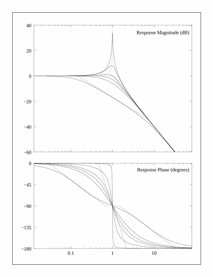
5.1. Plotting and charting: 2-D function plotting. This example showsa pair of associated function plots. These illlustrate the second-order re-sponse of a harmonic or control system. The response equation is

(1) Fc(s) =ω2n

s2 + 2cωns + ω2n

The plots are the magnitude and phase of this function against ω wheres = jω and the function is normalised with ωn = 1.

The six curves are for damping factors, c, of 0.01, 0.2, 0.5, 1/√

2, 1, and25/7. The asymptotes and tangents are shown for c = 0.5 and c = 25/7. Inthe latter overdamped case the magnitude response is close to the asymp-totes, the phase response is not close to the tangents. When overdamped, asecond-order system is essentially a combination of two separate first-ordersystems.


FIGURE 8. Second-order response curves. The magnitudeand phase response of a system for the damping factors 0.01,0.2, 0.5, 1/

√2, 1, and 25/7. Creation method: Octave, Gnu-

plot, XFig, ps output. Category: .

−60

−40

−20

0

20

40Response Magnitude (dB)

−180

−135

−90

−45

0

0.1 1 10

Response Phase (degrees)


5.2. Plotting and charting: 2-D statistical plotting. Statistical plots have alot of variety. Here we illustrate a fairly simple classification problem.

The idea is that we are given a set of training data in 2 classes and with2 observed (or feature) variables. We assume that the measurements arebivariate Gaussian (normal) distributions in each case, but that the param-eters are different in each case. The plot shows simulated data, and 2 of theellipses indicate the mean, variance and covariance estimated separatelyfor the 2 classes. Based on this a third ellipse has been drawn that passesbetween the others. A Bayesian interpretation is most straightforward. Us-ing as prior probabilities the relative frequencies of classes in the trainingset, measurements on this ellipse have equal posterior probability of beingin each of the 2 classes. For all other measurements, one class has a higherprobability than the other.


FIGURE 9. Bivariate 2-class classification. Training datapoints are shown, along with indicators of their distribution.The ellipse passing between the others divides the space ofobservation values for which each class has a higher poste-rior probability than the other. Creation method: Octave,eps output, with title and border added in XFig, ps output.Category: .

-12

-10

-8-6

-4-2

02

46

-6 -4 -2 0 2 4 6

Probabilistic Classification


5.3. Plotting and charting: Data charts and plots. This example is com-posed of three illustrations of drawing types used to convey business andeconomic information. The pie chart is standard. Note that under our def-inition the graph of frequency over time is a plot whereas the graph of fre-quency by price is a chart. The first incorporates a histogram. This has twoaxes, one being the interval scale time. The second is a bar chart whichrepresents categorical data and has distinct bars.

Even though one can draw formal distinctions between these drawings,they are typical of illustrations designed to convey a limited amount ofinformation with clarity and impact.

Although fictitious, the author’s (JAS’s) CD buying habits are reflectedsomewhat in this data. Naxos continues to expand its range of high-qualityclassical music at attractive prices, in contrast to most other labels. MostCDs normally at premium prices were only affordable at club (‘discount’)rates. This is not intended to be a product endorsement, but rather a criti-cism of other labels.


FIGURE 10. Presentation charts and plots. Illustrations offictitious CD buying habits. Creation method: XFig, ps out-put. Category: .

Discount

Very Low

Low

Medium

High

CD PurchasesOver Time

CD

s B

ou

gh

t

200

100

0

1.4

1.2

1.0

Lill

ipu

tian

Ret

ail P

rice

Ind

ex

��

��

��

��

� � � � � ��

� � � � � ��

��

��

0

50

100

150

200

250

Pre−1998 1998 1999 2000 2001 2002

Very L

ow

Lo

w

Mid

dle

Hig

h

Disco

un

tFrequency by PriceCD Purchasing Habits

Proportion by Genre

Falsified byJ Alex Stark

Classical

Cello

Early

Ro

man

tic/

mo

der

n

Bar

oq

ue

Price Key:


5.4. Plotting and charting: The virtual oscilloscope. To many readers thismay seem a rather minor use of a drawing program. However, the author(JAS) has found the tools for signal processing to be lacking. Application ar-eas for signal display include communications, audio and biomedical sys-tems.

This example illustrates two features that are not generally supported ina signal display:

• The display of two selections together. In this case a zoomed seg-ment is shown below another.

• The display of a processed segment or an analysis of a segmentalong side the original signal.

In addition to these features, one application of the Adage system might bea dynamic oscilloscope-type signal viewer. This would be able to producethe same kind of display but allow the user to scroll through interactively.


FIGURE 11. Patch-clamp record. A simulated signal withtwo C-O-C ion channels. The middle plot is a segment of theupper signal, and the lower plot shows a smoothed signaland indication of the envelope. Creation method: Octave,Gnuplot & XFig, ps output. Category: .

Time (s)

−1

0

1

2

3

20 25 30 35

Con

duct

ance

(pS

)

−1

0

1

2

3

29 29.5 30 30.5 31 31.5 32 32.5 33

Con

duct

ance

(pS

)

−1

0

1

2

3

29 29.5 30 30.5 31 31.5 32 32.5 33

Con

duct

ance

(pS

)


5.5. Plotting and charting: 3-D plotting. This plot shows the frequencywith which a simulated ion channel signal had segments with different con-ductances and durations. It is largely self-explanatory. It is not yet an aimof the Adage project to implement all the processes required to generatesuch a plot. Adage would be used as the rendering engine for a programthat can generate the contours from multidimensional data. Nevertheless,this could become part of the project.

The contours are plotted in an inappropriate dotted line because Gnuplotis incapable of producing anything better. A waterfall plot might have beenpreferred, but Gnuplot is also inadequate in this regard. A waterfall plot islike a mesh plot but with connecting lines in only one direction. Instead oflooking like a deformed grid, it is like a deformed striped carpet.


FIGURE 12. Histogram against durations and conduc-tances. The plot is of the frequency with which segmentsof a simulated ion channel signal had specific ranges of con-ductances and durations. Creation method: Octave, Gnu-plot & XFig, ps output. Category: .

−0.

50

0.5

11.

52

2.5

Con

duct

ance

(pS

)0.

1

1

10

100

0

100

200

300

400

500

the adage gallery tour i: highlights - …adage.sourceforge.net/doc/highlights/highlights.pdf ·...

Documents