the 2df galaxy redshift survey: wiener reconstruction of the
TRANSCRIPT

Mon. Not. R. Astron. Soc. 352, 939–960 (2004) doi:10.1111/j.1365-2966.2004.07984.x
The 2dF Galaxy Redshift Survey: Wiener reconstructionof the cosmic web
Pirin Erdogdu,1,2� Ofer Lahav,1,18 Saleem Zaroubi,3 George Efstathiou,1 Steve Moody,John A. Peacock,12 Matthew Colless,17 Ivan K. Baldry,9 Carlton M. Baugh,16
Joss Bland-Hawthorn,7 Terry Bridges,7 Russell Cannon,7 Shaun Cole,16 Chris Collins,4
Warrick Couch,5 Gavin Dalton,6,15 Roberto De Propris,17 Simon P. Driver,17
Richard S. Ellis,8 Carlos S. Frenk,16 Karl Glazebrook,9 Carole Jackson,17 Ian Lewis,6
Stuart Lumsden,10 Steve Maddox,11 Darren Madgwick,13 Peder Norberg,14
Bruce A. Peterson,17 Will Sutherland12 and Keith Taylor8 (the 2dFGRS Team)1Institute of Astronomy, Madingley Road, Cambridge CB3 0HA2Department of Physics, Middle East Technical University, 06531, Ankara, Turkey3Kapteyn Institute, University of Groningen, PO Box 800, 9700 AV, Groningen, the Netherlands4Astrophysics Research Institute, Liverpool John Moores University, Twelve Quays House, Birkenhead L14 1LD5Department of Astrophysics, University of New South Wales, Sydney, NSW 2052, Australia6Department of Physics, University of Oxford, Keble Road, Oxford OX1 3RH7Anglo-Australian Observatory, PO Box 296, Epping, NSW 2111, Australia8Department of Astronomy, California Institute of Technology, Pasadena, CA 91025, USA9Department of Physics and Astronomy, Johns Hopkins University, Baltimore, MD 21118-2686, USA10Department of Physics, University of Leeds, Woodhouse Lane, Leeds LS2 9JT11School of Physics and Astronomy, University of Nottingham, Nottingham NG7 2RD12Institute for Astronomy, University of Edinburgh, Royal Observatory, Blackford Hill, Edinburgh EH9 3HJ13Lawrence Berkeley National Laboratory, 1 Cyclotron Road, Berkeley, CA 94720, USA14ETHZ Institut fur Astronomie, HPF G3.1, ETH Honggerberg, CH-8093 Zurich, Switzerland15Rutherford Appleton Laboratory, Chilton, Didcot OX11 0QX16Department of Physics, University of Durham, South Road, Durham DH1 3LE17Research School of Astronomy and Astrophysics, The Australian National University, Weston Creek, ACT 2611, Australia18Department of Physics and Astronomy, University College London, Gower Street, London WC1E 6BT
Accepted 2004 May 3. Received 2004 April 30; in original form 2003 November 7
ABSTRACTWe reconstruct the underlying density field of the Two-degree Field Galaxy Redshift Survey(2dFGRS) for the redshift range 0.035 < z < 0.200 using the Wiener filtering method. TheWiener filter suppresses shot noise and accounts for selection and incompleteness effects.The method relies on prior knowledge of the 2dF power spectrum of fluctuations and thecombination of matter density and bias parameters, however the results are only slightly affectedby changes to these parameters. We present maps of the density field. We use a variablesmoothing technique with two different effective resolutions: 5 and 10 h−1 Mpc at the medianredshift of the survey. We identify all major superclusters and voids in the survey. In particular,we find two large superclusters and two large local voids. The full set of colour maps can beviewed on the World Wide Web at http://www.ast.cam.ac.uk/∼pirin.
Key words: methods: statistical – galaxies: distances and redshifts – large-scale structure ofUniverse.
�E-mail: [email protected]
C© 2004 RAS
940 P. Erdogdu et al.
1 I N T RO D U C T I O N
Historically, redshift surveys have provided the data and the testground for much of the research on the nature of clustering andthe distribution of galaxies. In the past few years, observations oflarge-scale structure have improved greatly. Today, with the devel-opment of fibre-fed spectrographs that can simultaneously measurespectra of hundreds of galaxies, cosmologists have at their finger-tips large redshift surveys such as Two-degree Field (2dF) and SloanDigital Sky Survey (SDSS). The analysis of these redshift surveysyields invaluable cosmological information. On the quantitativeside, with the assumption that the galaxy distribution arises from thegravitational instability of small fluctuations generated in the earlyUniverse, a wide range of statistical measurements can be obtained,such as the power spectrum and bispectrum. Furthermore, a qual-itative understanding of galaxy distribution provides insight intothe mechanisms of structure formation that generate the complexpattern of sheets and filaments comprising the ‘cosmic web’ (Bond,Kofman & Pogosyan 1996) we observe, and allows us to map a widevariety of structure, including clusters, superclusters and voids.
Today, many more redshifts are available for galaxies than directdistance measurements. This discrepancy inspired a great deal ofwork on methods for reconstruction of the real-space density fieldfrom that observed in redshift space. These methods use a varietyof functional representations (e.g. Cartesian, Fourier, spherical har-monics or wavelets) and smoothing techniques (e.g. a Gaussian or atop-hat sphere). There are physical as well as practical reasons whyone would be interested in smoothing the observed density field. Itis often assumed that the galaxy distribution samples the underlyingsmooth density field and the two are related by a proportionalityconstant, the so-called linear bias parameter, b. The finite samplingof the smooth underlying field introduces Poisson ‘shot noise’.1 Anyrobust reconstruction technique must reliably mitigate the statisticaluncertainties due to shot noise. Moreover, in redshift surveys, theactual number of galaxies in a given volume is larger than the num-ber observed, in particular in magnitude-limited samples where atlarge distances only very luminous galaxies can be seen.
In this paper, we analyse large-scale structure in the Two-degreeField Galaxy Redshift Survey (2dFGRS; Colless et al. 2001), whichhas now obtained the redshifts for approximately 230 000 galax-ies. We recover the underlying density field, characterized by anassumed power spectrum of fluctuations, from the observed fieldwhich suffers from incomplete sky coverage (described by the an-gular mask) and incomplete galaxy sampling due to its magnitudelimit (described by the selection function). The filtering is achievedby a Wiener filter (Wiener 1949; Press et al. 1992) within the frame-work of both linear and non-linear theory of density fluctuations.The Wiener filter is optimal in the sense that the variance betweenthe derived reconstruction and the underlying true density field isminimized. As opposed to ad hoc smoothing schemes, the smooth-ing due to the Wiener filter is determined by the data. In the limitof high signal-to-noise, the Wiener filter modifies the observed dataonly weakly, whereas it suppresses the contribution of the data con-taminated by shot noise.
Wiener filtering is a well-known technique and has been appliedto many fields in astronomy (see Rybicki & Press 1992). For ex-
1 Another popular model for galaxy clustering is the halo model where thelinear bias parameter depends on the mass of the dark matter haloes wherethe galaxies reside. For this model, the mean number of galaxy pairs in agiven halo is usually lower than the Poisson expectation.
ample, the method was used to reconstruct the angular distribution(Lahav et al. 1994), the real-space density, velocity and gravitationalpotential fields of the 1.2-Jy IRAS (Fisher et al. 1995) and IRAS PSCzsurveys (Schmoldt et al. 1999). The Wiener filter was also appliedto the reconstruction of the angular maps of the cosmic microwavebackground temperature fluctuations (Bunn et al. 1994; Tegmark &Efstathiou 1996; Bouchet & Gispert 1999). A detailed formalism ofthe Wiener filtering method as it pertains to the large-scale structurereconstruction can be found in Zaroubi et al. (1995).
This paper is structured as follows. We begin with a brief reviewof the formalism of the Wiener filter method. A summary of the2dFGRS data set, the survey mask and the selection function aregiven in Section 3. In Section 4, we outline the scheme used topixelize the survey. In Section 5, we give the formalism for thecovariance matrix used in the analysis. After that, we describe theapplication of the Wiener filter method to the 2dFGRS and presentdetailed maps of the reconstructed field. In Section 7, we identifythe superclusters and voids in the survey.
Throughout this paper, we assume a � cold dark matter (CDM)cosmology with �m = 0.3 and �� = 0.7 and H 0 = 100 h−1 kms−1 Mpc−1.
2 W I E N E R F I LT E R
In this section, we give a brief description of the Wiener filtermethod. For more details, we refer the reader to Zaroubi et al.(1995). Let us assume that we have a set of measurements, {d α}(α =1, 2, . . . N ) which are a linear convolution of the true underlyingsignal, sα , plus a contribution from statistical noise, εα , such that
dα = sα + εα. (1)
The Wiener filter is defined as the linear combination of the observeddata, which is closest to the true signal in a minimum variance sense.More explicitly, the Wiener filter estimate, sWF
α , is given by sWFα =
F αβ d β where the filter is chosen to minimize the variance of theresidual field, rα:⟨∣∣r 2
α
∣∣⟩ =⟨∣∣sWF
α − sα
∣∣2⟩
. (2)
It is straightforward to show that the Wiener filter is
Fαβ = ⟨sαd†
γ
⟩⟨dγ d†
β
⟩−1, (3)
where the first term on the right-hand side is the signal–data corre-lation matrix⟨
sαd†γ
⟩ = ⟨sαs†γ
⟩, (4)
and the second term is the data–data correlation matrix⟨dαd†
β
⟩ = ⟨sγ s†δ
⟩ + ⟨εαε
†β
⟩. (5)
In the above equations, we have assumed that the signal and noiseare uncorrelated. From equations (3) and (5), it is clear that, in orderto implement the Wiener filter, one must construct a prior whichdepends on the mean of the signal (which is zero by construction)and the variance of the signal and noise. The assumption of a priormay be alarming at first glance. However, slightly inaccurate val-ues of Wiener filter will only introduce second-order errors to thefull reconstruction (see Rybicki & Press 1992). The dependence ofthe Wiener filter on the prior can be made clear by defining signaland noise matrices as C αβ = 〈sαs†β〉 and N αβ = 〈εαε
†β〉. With this
C© 2004 RAS, MNRAS 352, 939–960

2dFGRS: Wiener reconstruction of the cosmic web 941
notation, we can rewrite the equations above so that sWF is given as
sWF = C [C + N]−1 d. (6)
The mean square residual given in equation (2) can then be calcu-lated as
〈rr†〉 = C [C + N]−1 N. (7)
Formulated in this way, we see that the purpose of the Wiener filteris to attenuate the contribution of low signal-to-noise ratio data. Thederivation of the Wiener filter given above follows from the solerequirement of minimum variance and requires only a model forthe variance of the signal and noise. The Wiener filter can also bederived using the laws of conditional probability if the underlyingdistribution functions for the signal and noise are assumed to beGaussian. For the Gaussian prior, the Wiener filter estimate is boththe maximum posterior estimate and the mean field (see Zaroubiet al. 1995).
As several authors point out (e.g. Rybicki & Press 1992; Zaroubi2002), the Wiener filter is a biased estimator because it predicts anull field in the absence of good data, unless the field itself has zeromean. Because we have constructed the density field to have zeromean, we are not worried about this bias. However, the observedfield deviates from zero due to selection effects and so it is necessaryto be aware of this bias in the reconstructions.
It is well known that the peculiar velocities of galaxies distortclustering pattern in redshift space. On small scales, the randompeculiar velocity of each galaxy causes smearing along the line ofsight, known as the Finger of God. On larger scales, there is com-pression of structures along the line of sight due to coherent infallvelocities of large-scale structure induced by gravity. One of themajor difficulties in analysing redshift surveys is the transformationof the position of galaxies from redshift space to real space. For allsky surveys, this issue can be addressed using several methods, forexample the iterative method of Yahil, Strauss & Huchra (1991) andthe modified Poisson equation of Nusser & Davis (1994). However,these methods are not applicable to surveys which are not all-sky asthey assume that, in linear theory, the peculiar velocity of any galaxyis a result of the matter distribution around it, and the gravitationalfield is dominated by the matter distribution inside the volume ofthe survey. For a survey such as the 2dFGRS, within the limitationof linear theory where the redshift-space density is a linear trans-formation of the real-space density, a Wiener filter can be used totransform from redshift space to real space (see Fisher et al. 1995and Zaroubi et al. 1995 for further details). This can be written as
sWF(rα) = 〈s(rα)d(sγ )〉〈d(sγ )d(sβ )〉−1d(sβ ), (8)
where the first term on the right-hand side is the cross-correlationmatrix of real- and redshift-space densities and s(r ) is the positionvector in redshift space. It is worth emphasizing that this method islimited. Although the Wiener filter has the ability to extrapolate thepeculiar velocity field beyond the boundaries of the survey, it stillonly recovers the field generated by the mass sources representedby the galaxies within the survey volume. It does not account forpossible external forces outside the range of the extrapolated field.This limitation can only be overcome by comparing the 2dF surveywith all sky surveys.
3 DATA
3.1 2dFGRS data
The 2dFGRS, now completed, is selected in the photometric bJ
band from the Automated Plate Measuring (APM) galaxy survey
(Maddox, Efstathiou & Sutherland 1990) and its subsequent ex-tensions. The survey covers about 2000 deg2 and is made upof two declination strips, one in the South Galactic Pole region(SGP) covering approximately −37.◦5 < δ < −22.◦5, 325.◦0 <
α < 55.◦0 and the other in the direction of the North GalacticPole (NGP), spanning −7.◦5 < δ < 2.◦5, 147.◦5 < α < 222.◦5. Inaddition to these contiguous regions, there are a number of ran-domly located circular two-degree fields scattered over the fullextent of the low-extinction regions of the southern APM galaxysurvey.
The magnitude limit at the start of the survey was set atbJ = 19.45 but both the photometry of the input catalogue andthe dust extinction map have been revised since. So, there are smallvariations in magnitude limit as a function of position over the sky,which are taken into account using the magnitude limit mask. Theeffective median magnitude limit, over the area of the survey, is bJ
≈ 19.3 (Colless et al. 2001).We use the data obtained prior to 2002 May, when the survey was
nearly complete. This includes 221 283 unique, reliable galaxy red-shifts. We analyse a magnitude-limited sample with redshift limitszmin = 0.035 and zmax = 0.20. The median redshift is zmed ≈ 0.11.We use 167 305 galaxies in total, 98 129 in the SGP and 69 176 inthe NGP. We do not include the random fields in our analysis.
The 2dFGRS data base and full documentation are available onthe WWW at http://www.mso.anu.edu.au/2dFGRS/.
3.2 Mask and radial selection function of the 2dFGRS
The completeness of the survey varies according to the position inthe sky due to unobserved fields, particularly at the survey edges,and unfibred objects in the observed fields because of collision con-straints or broken fibres.
For our analysis, we make use of two different masks (Collesset al. 2001; Norberg et al. 2002). The first of these masks is theredshift completeness mask defined as the ratio of the number ofgalaxies for which redshifts have been measured to the total numberof objects in the parent catalogue. This spatial incompleteness isillustrated in Fig. 1. The second mask is the magnitude limit maskwhich gives the extinction corrected magnitude limit of the surveyat each position.
The radial selection function gives the probability of observing agalaxy for a given redshift and can be readily calculated from thegalaxy luminosity function:
(L) dL = ∗(
L
L∗
)α
exp
(− L
L∗
)dL
L∗ . (9)
Here, for the concordance model, α = −1.21 ± 0.03, log10 L ∗ =−0.4 (−19.66 ± 0.07 + 5 log10(h)) and ∗ = 0.0161 ± 0.0008 h3
(Norberg et al. 2002).The selection function can then be expressed as
φ(r ) =∫ ∞
L(r ) (L) dL∫ ∞
Lmin (L) dL
, (10)
where L(r) is the minimum luminosity detectable at luminosity dis-tance r (assuming the concordance model), evaluated for the con-cordance model, L min = Min[L(r ), L com] and Lcom is the minimumluminosity for which the catalogue is complete and varies as a func-tion of position over the sky. For distances considered in this paper,where the deviations from the Hubble flow are relatively small, theselection function can be approximated as φ(r ) ≈ φ(zgal). Each
C© 2004 RAS, MNRAS 352, 939–960

942 P. Erdogdu et al.
Figure 1. The redshift completeness masks for the NGP (top) and SGP (bottom) in equatorial coordinates. The grey-scale shows the completeness fraction.
galaxy, gal, is then assigned the weight
w(gal) = 1
φ(zgal)M(�i )(11)
where φ(zgal) and M(�i) are the values of the selection function foreach galaxy and angular survey mask for each cell i (see Section 4),respectively.
4 S U RV E Y P I X E L I Z AT I O N
In order to form a data vector of overdensities, the survey needsto be pixelized. There are many ways to pixelize a survey: equalsized cubes in redshift space, igloo cells, spherical harmonics,Delauney tessellation methods, wavelet decomposition, etc. Eachof these methods has its own advantages and disadvantages, andthey should be treated with care as they form functional bases inwhich all the statistical and physical properties of cosmic fields areretained.
The pixelization scheme used in this analysis is an ‘igloo’ gridwith wedge-shaped pixels in Cartesian space. Each pixel is boundedin right ascension, declination and redshift. The pixelization is con-structed to keep the average number density per pixel approximatelyconstant. The advantage of using this pixelization is that the numberof pixels is minimized because the pixel volume is increased withredshift to counteract the decrease in the selection function. Thisis achieved by selecting a ‘target cell width’ for cells at the meanredshift of the survey and deriving the rest of the bin widths so asto match the shape of the selection function. The target cell widths
Figure 2. An illustration of the survey pixelization scheme used in theanalysis, for 10 h−1 Mpc (top) and 5 h−1 Mpc (bottom) target cell widths.The redshift ranges are given on the top of each plot.
used in this analysis are 10 and 5 h−1 Mpc. Once the redshift binninghas been calculated, each radial bin is split into declination bandsand then each band in declination is further divided into cells in rightascension. The process is designed so as to make the cells roughlycubical. Finally, the cell boundaries are converted to Cartesian co-ordinates for the analysis. In Fig. 2, we show an illustration of themethod by plotting the cells in right ascension and declination for agiven redshift strip.
C© 2004 RAS, MNRAS 352, 939–960

2dFGRS: Wiener reconstruction of the cosmic web 943
Although advantageous in many ways, the pixelization schemeused in this paper may complicate the interpretation of the recon-structed field. By definition, the Wiener filter signal will approachzero at the edges of the survey where the shot noise may dominate.This means the true signal will be constructed in a non-uniform man-ner. This effect will be amplified as the cell sizes become bigger athigher redshifts. Hence, both of these effects must be consideredwhen interpreting the results.
5 E S T I M AT I N G T H E S I G NA L – S I G NA LC O R R E L AT I O N M AT R I X OV E R P I X E L S
The signal covariance matrix can be accurately modelled byan analytical approximation (Moody 2003). The calculation ofthe covariance matrix is similar to the analysis described byEfstathiou & Moody (2001) apart from the modification due to three-dimensionality of the survey. The covariance matrix for the ‘noise-free’ density fluctuations is 〈Cij〉 = 〈δ iδ j 〉, where δ i = (ρi − ρ)/ρin the ith pixel. It is estimated by first considering a pair of pixelswith volumes Vi and Vj, separated by distance r so that
〈Ci j 〉 =⟨
1
Vi Vj
∫Celli
δ(x) dVi
∫Cell j
δ(x + r ) dVj
⟩(12)
= 1
Vi Vj
∫Celli
∫Cell j
〈δ(x)δ(x + r )〉 dVi dVj (13)
= 1
Vi Vj
∫Celli
∫Cell j
ξ (r ) dVi dVj (14)
where the isotropic two point correlation function ξ (r ) is given by
ξ (r ) = 1
(2π)3
∫P(k)e−ik·r d3k, (15)
and therefore,
〈Ci j 〉 = 1
(2π)3Vi Vj
∫P(k) d3k
×∫
Celli
∫Cell j
e−ik(r i −r j ) dVi dVj . (16)
After performing the Fourier transform, this equation can be writtenas
〈Ci j 〉 = 1
(2π)3
∫P(k)S(k, Li )S(k, L j )C(k, r ) d3k, (17)
where the functions S and C are given by
S(k, L) = sinc(kx Lx/2)sinc(ky L y/2)sinc(kz Lz/2) (18)
C(k, r ) = cos(kxrx ) cos(kyry) cos(kzrz). (19)
Here, the label L describes the dimensions of the cell (Lx, Ly, Lz),the components of r describe the separation between cell centres,k = (kx, ky, kz) is the wave vector and sinc(x) = (sin(x))/x . Thewave vector, k, is written in spherical coordinates k, θ , φ to simplifythe evaluation of C. We define
kx =k sin(φ) cos(θ ) (20)
ky =k sin(φ) sin(θ ) (21)
kz =k cos(φ). (22)
Equation (17) can now be integrated over θ and φ to form the kernelGij (k) where
Gi j (k) = 1
π3
∫ π/2
0
∫ π/2
0
S(k, Li )S(k, L j )C(k, r )
× sin(φ) dθ dφ, (23)
so that
〈Ci j 〉 =∫
P(k)Gi j (k)k2 dk. (24)
In practice, we evaluate
〈Ci j 〉 =∑
k
Pk Gi jk, (25)
where Pk is the binned bandpower spectrum and Gijk is
Gi jk =∫ kmax
kmin
Gi j (k) k2 dk, (26)
where the integral extends over the band corresponding to the bandpower Pk.
For cells that are separated by a distance much larger than the celldimensions, the cell window functions can be ignored, simplifyingthe calculation so that
Gi jk = 1
(2π)3
∫ kmax
kmin
sinc(kr ) 4πk2 dk, (27)
where r is the separation between cell centres.
6 A P P L I C AT I O N
6.1 Reconstruction using linear theory
In order to calculate the data vector d in equation (6), we first estimatethe number of galaxies Ni in each pixel i
Ni =Ngal(i)∑
gal
w(gal), (28)
where the sum is over all the observed galaxies in the pixel andw(gal) is the weight assigned to each galaxy (equation 11). Theboundaries of each pixel are defined by the scheme described inSection 4, using a target cell width of 10 h−1 Mpc. There are 13 480cells in total (4526 in the NGP and 8954 in the SGP). The meannumber of galaxies in pixel i is
Ni = nVi , (29)
where Vi is the volume of the pixel and the mean galaxy density, n,is estimated using the equation
n =∑Ntotal
gal w(gal)∫ ∞0
drr 2φ(r )w(r ), (30)
where the sum is now over all the galaxies in the survey. We notethat the value for n obtained using the equation above is consistentwith the maximum estimator method proposed by Davis & Huchra(1982). Using these definitions, we write the ith component of thedata vector d as
di = Ni − Ni
Ni. (31)
Note that the mean value of d is zero by construction.Reconstruction of the underlying signal given in equation (6)
also requires the signal–signal and the inverse of the data–data
C© 2004 RAS, MNRAS 352, 939–960

944 P. Erdogdu et al.
correlation matrices. The data–data correlation matrix (equation 5)is the sum of noise–noise correlation matrix N and the signal–signalcorrelation matrix C formulated in the previous section. The onlychange made is to the calculation of C where the real-space corre-lation function ξ (r ) is now multiplied by the Kaiser factor in orderto correct for the redshift distortions on large scales. So
ξs = 1
(2π)3
∫PS(k) exp[ik · (r2 − r1)] d3k, (32)
where PS(k) is the galaxy power spectrum in redshift space
PS(k) = K [β]PR(k), (33)
derived in linear theory. The superscripts ‘R’ and ‘S’ in this equation(and hereafter) denote real and redshift space, respectively.
K [β] = 1 + 2
3β + 1
5β2 (34)
is the direction averaged Kaiser (1987) factor, derived using a dis-tant observer approximation and with the assumption that the datasubtend a small solid angle with respect to the observer (the latterassumption is valid for the 2dFGRS but does not hold for a wideangle survey; see Zaroubi & Hoffman, 1996 for a full discussion).Equation (33) shows that, in order to apply the Wiener filter method,we need a model for the galaxy power spectrum in redshift spacewhich depends on the real-space power spectrum and on the redshiftdistortion parameter, β ≡ �0.6
m /b.The real-space galaxy power spectrum is well described by a
scale invariant CDM power spectrum with shape parameter, �, forthe scales concerned in this analysis. For �, we use the value derivedfrom the 2dF survey by Percival et al. (2001) who fitted the 2dFGRSpower spectrum over the range of linear scales using the fittingformulae of Eisenstein & Hu (1998). Assuming a Gaussian prior onthe Hubble constant h = 0.7 ± 0.07 (based on Freedman et al. 2001),they find � = 0.2 ± 0.03. The normalization of the power spectrumis conventionally expressed in terms of the variance of the densityfield in spheres of 8 h−1 Mpc, σ 8. Lahav et al. (2002) use 2dFGRSdata to deduce σ S
8g(L s, z s) = 0.94 ± 0.02 for the galaxies in redshiftspace, assuming h = 0.7 ± 0.07 at z s ≈ 0.17 and L s ≈ 1.9L∗. Weconvert this result to real space using the following equation
σ R8g(L s, zs) = σ S
8g(L s, zs)/K 1/2[β(L s, zs)] (35)
where K[β] is the Kaiser factor. For our analysis, we need to useσ 8 evaluated at the mean redshift of the survey for galaxies withluminosity L∗. However, it is necessary to assume a model for theevolution of galaxy clustering in order to find σ 8 at different red-shifts. Moreover, the conversion from Ls to L∗ introduces uncertain-ties in the calculation. Therefore, we choose an approximate value,σ R
8g ≈ 0.8 to normalize the power spectrum. For β, we adopt thevalue found by Hawkins et al. (2003), β(L s, z s) = 0.49 ± 0.09which is estimated at the effective luminosity, L s ≈ 1.4L∗, and theeffective redshift, z s ≈ 0.15, of the survey sample. Our results arenot sensitive to minor changes in σ 8 and β.
The other component of the data–data correlation matrix is thenoise correlation matrix N. Assuming that the noise in differentcells is not correlated, the only non-zero terms in N are the diagonalterms given by the variance – the second central moment – of thedensity error in each cell:
Ni i = 1
N 2i
Ngal(i)∑gal
w2(gal). (36)
The final aspect of the analysis is the reconstruction of the real-space density field from the redshift-space observations. This isachieved using equation (8). Following Kaiser (1987), using dis-
tant observer and small-angle approximation, the cross-correlationmatrix in equation (8) for the linear regime can be written as
〈s(r )d(s)〉 = 〈δrδs〉 = ξ (r )
(1 + 1
3β
), (37)
where s and r are position vectors in redshift and real space, respec-tively. The term (1 + (1/3)β) is easily obtained by integrating thedirection-dependent density field in redshift space. Using equation(37), the transformation from redshift space to real space simplifiesto
sWF(r ) = 1 + (1/3)β
K [β]C [C + N]−1 d. (38)
As mentioned earlier, the equation above is calculated for linearscales only and hence small-scale distortions (i.e. Fingers of God)are not corrected for. For this reason, we collapse in redshift spacethe fingers seen in 2dF groups (Eke et al. 2003) with more than 75members, 25 groups in total (11 in the NGP and 14 in the SGP). Allthe galaxies in these groups are assigned the same coordinates. Asexpected, correcting these small-scale distortions does not changethe constructed fields substantially as these distortions are practi-cally smoothed out because of the cell size used in binning the data.
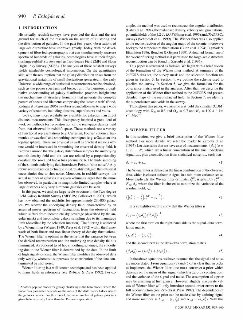
The maps shown in this section were derived by the techniquedetailed above. There are 80 sets of plots which show the densityfields as strips in RA and Dec., 40 maps for the SGP and 40 mapsfor the NGP. Here we just show some examples; the rest of the plotscan be found at http://www.ast.cam.ac.uk/∼pirin. For comparison,the top plots of Figs 3, 4, 5 and 6 show the redshift-space densityfield weighted by the selection function and the angular mask. Thecontours are spaced at �δ = 0.5 with solid (dashed) lines denotingpositive (negative) contours; the heavy solid contours correspondto δ = 0. Also plotted for comparison are the galaxies (dots) andthe groups with N gr number of members (Eke et al. 2003) and 9� N gr � 17 (circles), 18 � N gr � 44 (squares) and 45 � N gr
(stars). We also show the number of Abell, APM and Edinburgh–Durham Cluster Catalogue (EDCC) clusters studied by De Propriset al. (2002) (upside-down triangles). The middle plots show theredshift-space density shown in top plots after the Wiener filter isapplied. As expected, the Wiener filter suppresses the noise. Thesmoothing performed by the Wiener filter is variable and increaseswith distance. The bottom plots show the reconstructed real densityfield sWF(r ), after correcting for the redshift distortions. Here theamplitude of density contrast is reduced slightly. We also plot thereconstructed fields in declination slices. These plots are shown inFigs 7 and 8.
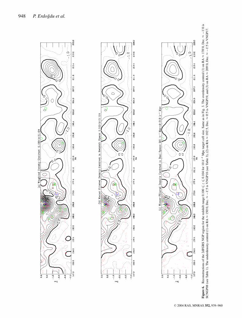
We also plot the square root of the variance of the residual field(equation 2), which defines the scatter around the mean recon-structed field. We plot the residual fields corresponding to someof the redshift slices shown in this paper (Figs 9 and 10). For bettercomparison, plots are made so that the cell number increases withincreasing RA. If the volume of the cells used to pixelize the surveywas constant, we would expect the square root of the variance �δ
to increase due to the increase in shot noise (equation 7). However,because the pixelization was constructed to keep the shot noise perpixel approximately constant, �δ also remains constant (�δ ≈ 0.23for both the NGP and SGP) but the average density contrast in eachpixel decreases with increasing redshift. This means that, althoughthe variance of the residual in each cell is roughly equal, the relativevariance (represented by �δ/δ) increases with increasing redshift.This increase is clearly evident in Figs 9 and 10. Another conclusionthat can be drawn from the figures is that the bumps in the densityfield are due to real features not due to error in the reconstruction,even at higher redshifts.
C© 2004 RAS, MNRAS 352, 939–960

2dFGRS: Wiener reconstruction of the cosmic web 945
Fig
ure
3.R
econ
stru
ctio
nsof
the
2dFG
RS
SGP
regi
onfo
rth
ere
dshi
ftra
nge
0.05
7�
z�
0.06
1fo
r10
h−1
Mpc
targ
etce
llsi
ze.T
heco
ntou
rsar
esp
aced
at�
δ=
0.5
with
solid
(das
hed)
lines
deno
ting
posi
tive
(neg
ativ
e)co
ntou
rs;t
hehe
avy
solid
cont
ours
corr
espo
ndto
δ=
0.T
hedo
tsde
note
the
gala
xies
with
reds
hift
sin
the
plot
ted
rang
e.(a
)R
edsh
ift-
spac
ede
nsity
field
wei
ghte
dby
the
sele
ctio
nfu
nctio
nan
dth
ean
gula
rm
ask.
(b)
Sam
eas
in(a
)bu
tsm
ooth
edby
aW
iene
rfil
ter.
(c)
Sam
eas
in(b
)bu
tcor
rect
edfo
rth
ere
dshi
ftdi
stor
tion.
The
over
dens
ityce
ntre
d(1
)on
RA
≈33
6.◦5,
Dec
.≈−3
0.◦0
isSC
SGP0
3(s
eeTa
ble
1),(
2)on
RA
≈0.◦
0,D
ec.≈
−30.◦
0is
SCSG
P04
(thi
sov
erde
nsity
ispa
rtof
the
Pisc
es–C
etus
supe
rclu
ster
,and
(3)
onR
A≈
36.◦ 0
,Dec
.≈−2
9.◦3
isSC
SGP0
5.T
heun
derd
ensi
tyce
ntre
don
RA
≈35
0.◦0,
Dec
.≈−3
0.◦0
isV
SGP1
2(s
eeTa
ble
2).
C© 2004 RAS, MNRAS 352, 939–960

946 P. Erdogdu et al.
Fig
ure
4.R
econ
stru
ctio
nsof
the
2dFG
RS
SGP
regi
onfo
rth
ere
dshi
ftra
nge
0.06
8�
z�
0.07
1fo
r10
h−1
Mpc
targ
etce
llsi
ze.S
ame
asin
Fig.
3.T
heov
erde
nsity
cent
red
(1)
onR
A≈
39.◦ 0
,Dec
.≈−3
4.◦5
isSC
SGP0
7(s
eeTa
ble
1)an
dis
part
ofth
eL
eo–C
oma
supe
rclu
ster
,and
(2)
onR
A≈
0.◦0,
Dec
.≈−3
0.◦0
isSC
SGP0
6an
dis
part
ofH
orog
lium
Ret
icul
umsu
perc
lust
er(s
eeTa
ble
1).
C© 2004 RAS, MNRAS 352, 939–960

2dFGRS: Wiener reconstruction of the cosmic web 947
Fig
ure
5.R
econ
stru
ctio
nsof
the
2dFG
RS
NG
Pre
gion
for
the
reds
hift
rang
e0.
082
�z
�0.
086
for
10h−
1M
pcta
rget
cell
size
.Sa
me
asin
Fig.
3.T
heov
erde
nsity
cent
red
onR
A≈
194.◦
0,D
ec.≈
−2.◦ 5
isSC
NG
P06
(see
Tabl
e1)
.
C© 2004 RAS, MNRAS 352, 939–960
948 P. Erdogdu et al.
Fig
ure
6.R
econ
stru
ctio
nsof
the
2dFG
RS
NG
Pre
gion
for
the
reds
hift
rang
e0.
100
�z
�0.
104
for
10h−
1M
pcta
rget
cell
size
.Sam
eas
inFi
g.3.
The
over
dens
ityce
ntre
d(1
)on
RA
≈17
0.◦0,
Dec
.≈−1
.◦ 0is
SCN
GP0
8(s
eeTa
ble
1).T
heun
derd
ensi
tyce
ntre
d(1
)on
RA
≈15
0.◦0,
Dec
.≈−1
.◦ 5is
VN
GP1
8(s
eeTa
ble
3),(
2)on
RA
≈19
2.◦5,
Dec
.≈0.◦
5is
VN
GP1
9,an
d(3
)on
RA
≈20
9.◦0,
Dec
.≈−1
.◦ 5is
VN
GP1
7.
C© 2004 RAS, MNRAS 352, 939–960

2dFGRS: Wiener reconstruction of the cosmic web 949
Figure 7. Reconstructions of the 2dFGRS SGP region in slices of declination for 10 h−1 Mpc target cell size. The declination range is given on the top ofeach plot. The contours are spaced at �δ = 1.0 with solid (dashed) lines denoting positive (negative) contours; the heavy solid contours correspond to δ = 0.
We also use the χ2 statistic in order to check the consistency ofthe model with the data. χ2 is defined by
χ 2 = d†(S + N)−1d. (39)
A value χ 2 that is of the order of the number of degrees of free-dom (dof) means that the model and the data are consistent. In thisanalysis, the number of dof equals the number of pixels. We findχ2/dof = 1.06. This value indicates that the data and the model arein very good agreement.
6.2 Reconstruction using non-linear theory
In order to increase the resolution of the density field maps, wereduce the target cell width to 5 h−1 Mpc. A volume of a cubic cell
of side 5 h−1 Mpc is roughly equal to a top-hat sphere of radius ofabout 3 h−1 Mpc. The variance of the mass density field in this sphereis σ 3 ≈ 1.7 which corresponds to non-linear scales. To reconstructthe density field on these scales, we require accurate descriptionsof the non-linear galaxy power spectrum and the non-linear redshiftspace distortions.
For the non-linear matter power spectrum PRnl(k), we adopt the
empirical fitting formula of Smith et al. (2003). This formula, de-rived using the ‘halo model’ for galaxy clustering, is more accuratethan the widely used Peacock & Dodds (1996) fitting formula, whichis based on the assumption of ‘stable clustering’ of virialized haloes.We note that for the scales concerned in this paper (up to k ≈ 10 hMpc−1), Smith et al. (2003) and Peacock & Dodds (1996) fittingformulae give very similar results. For simplicity we assume linear,
C© 2004 RAS, MNRAS 352, 939–960
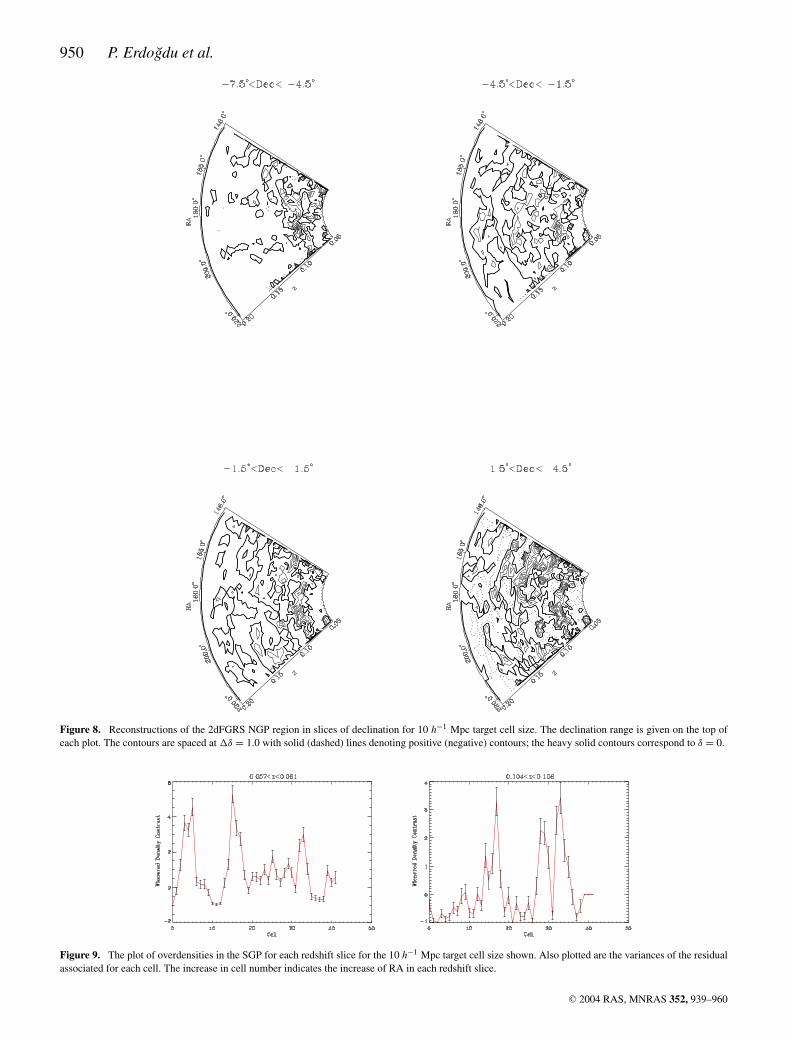
950 P. Erdogdu et al.
Figure 8. Reconstructions of the 2dFGRS NGP region in slices of declination for 10 h−1 Mpc target cell size. The declination range is given on the top ofeach plot. The contours are spaced at �δ = 1.0 with solid (dashed) lines denoting positive (negative) contours; the heavy solid contours correspond to δ = 0.
Figure 9. The plot of overdensities in the SGP for each redshift slice for the 10 h−1 Mpc target cell size shown. Also plotted are the variances of the residualassociated for each cell. The increase in cell number indicates the increase of RA in each redshift slice.
C© 2004 RAS, MNRAS 352, 939–960

2dFGRS: Wiener reconstruction of the cosmic web 951
Figure 10. Same as in Fig. 9 but for the redshift slices in the NGP shown above.
scale-independent biasing in order to determine the galaxy powerspectrum from the mass power spectrum, where b measures the ratiobetween galaxy and mass distribution:
PRnl (k) = b2 Pm
nl (k). (40)
Here, PRnl(k) is the galaxy and Pm
nl(k) is the matter power spectrum.We assume that b = 1.0 for our analysis. While this value is inagreement with the result obtained from the 2dFGRS (Lahav et al.2002; Verde et al. 2002) for scales of tens of Mpc, it does not hold truefor the scales of 5 h−1 Mpc on which different galaxy populationsshow different clustering patterns Madgwick et al. 2002; Norberget al. 2002; Zehavi et al. 2002). More realistic models exist wherebiasing is scale-dependent (e.g. Peacock & Smith 2000; Seljak 2000)but because the Wiener filtering method is not sensitive to smallerrors in the prior parameters and the reconstruction scales are nothighly non-linear, the simple assumption of no bias will still giveaccurate reconstructions.
The main effect of redshift distortions on non-linear scales is thereduction of power as a result of radial smearing due to virializedmotions. The density profile in redshift space is then the convolutionof its real-space counterpart with the peculiar velocity distributionalong the line of sight, leading to damping of power on small scales.This effect is known to be reasonably well approximated by treatingthe pairwise peculiar velocity field as Gaussian or better still as anexponential in real space (superpositions of Gaussians), with disper-sion σ p (e.g. Peacock & Dodds 1994; Ballinger, Peacock & Heavens1996; Kang et al. 2002). Therefore the galaxy power spectrum inredshift space is written as
PSnl(k, µ) = PR
nl (k, µ)(1 + βµ2)2 D(kσpµ), (41)
where µ is the cosine of the wave vector to the line of sight, σ p
has the unit of h−1 Mpc and the damping function in k-space is aLorentzian:
D(kσpµ) = 1
1 + (k2σ 2
p µ2)/
2. (42)
Integrating equation (41) over µ, we obtain the direction-averagedpower spectrum in redshift space:
PSnl(k)
PRnl (k)
=4(σ 2
p k2 − β
)β
σ 4p k4
+ 2β2
3σ 2p k2
+√
2(
k2σ 2p − 2β
)2arctan(kσp/
√2)
k5σ 5p
.(43)
For the non-linear reconstruction, we use equation (43) instead ofequation (33) when deriving the correlation function in redshiftspace. Fig. 11 shows how the non-linear power spectrum is dampedin redshift space (dashed line) and compared to the linear power
Figure 11. Non-linear power spectra for z = 0 and the concordance modelwith σ p = 506 km s−1 in real space (solid line), in redshift space fromequation (43) (dashed line), both derived using the fitting formulae of Smithet al. (2003) and linear power spectra in redshift space derived using lineartheory and the Kaiser factor (dotted line).
spectrum (dotted line). In this plot and throughout this paper weadopt the σ p value derived by Hawkins et al. (2003), σ p = 506 ±52 km s−1. Interestingly, by coincidence, the non-linear and linearpower spectra look very similar in redshift space. So, if we had usedthe linear power spectrum instead of its non-linear counterpart, westill would have obtained physically accurate reconstructions of thedensity field in redshift space.
The optimal density field in real space is calculated usingequation (8). The cross-correlation matrix in equation (38) can nowbe approximated as
〈s(r )d(s)〉 = ξ (r , µ)(1 + βµ2)√
D(kσpµ). (44)
Again, integrating the equation above over µ, the direction averagedcross-correlation matrix of the density field in real space and thedensity field in redshift space can be written as
〈s(r ) d(s)〉〈s(r ) s(r )〉 = 1
2k2σ 2p
ln[
k2σ 2p
(1 +
√1 + 1/k2σ 2
p
)]+ β
k2σ 2p
√1 + k2σ 2
p + β
k3σ 3p
arcsinh(
k2σ 2p
). (45)
In this paper, we show some examples of the non-linear recon-structions (Figs 12 , 13, 14 and 15). As can be seen from these plots,the resolution of the reconstructions improves radically, down to thescale of large clusters. Comparing Figs 6 and 15 where the redshift
C© 2004 RAS, MNRAS 352, 939–960

952 P. Erdogdu et al.
Fig
ure
12.
Rec
onst
ruct
ions
ofth
e2d
FGR
SSG
Pre
gion
fort
here
dshi
ftra
nge
0.04
7�
z�
0.04
9fo
r5h−
1M
pcta
rget
cell
size
.The
over
dens
ityce
ntre
d(1
)on
RA
≈33
6.◦5,
Dec
.≈−3
0.◦0
isSC
SGP0
3(s
eeTa
ble
1),
(2)
onR
A≈
0.◦0,
Dec
.≈−3
0.◦0
isSC
SGP0
4,an
d(3
)on
RA
≈36
.◦ 0,D
ec.≈
−29.◦
3is
SCSG
P05.
The
unde
rden
sity
cent
red
(1)
onR
A≈
339.◦
5,D
ec.≈
−30.◦
0is
VSG
P01,
(2)
onR
A≈
351.◦
5,D
ec.≈
−29.◦
3is
VSG
P02,
(3)
onR
A≈
18.◦ 0
,Dec
.≈−2
8.◦5
isV
SGP0
4,an
d(4
)on
RA
≈32
.◦ 2,D
ec.≈
−29.◦
5is
VSG
P05
(see
Tabl
e2)
.
C© 2004 RAS, MNRAS 352, 939–960

2dFGRS: Wiener reconstruction of the cosmic web 953
Fig
ure
13.
Rec
onst
ruct
ions
ofth
e2d
FGR
SSG
Pre
gion
for
the
reds
hift
rang
e0.
107
�z
�0.
108
for
5h−
1M
pcta
rget
cell
size
.Sam
eas
inFi
g.3.
The
over
dens
ityce
ntre
d(1
)on
RA
≈1.◦
7,D
ec.≈
−31.◦
0is
SCSG
P16
(see
Tabl
e1)
,(2)
onR
A≈
36.◦ 3
,Dec
.≈−3
0.◦0
isSC
SGP1
5,an
d(3
)on
RA
≈34
5.◦0,
Dec
.≈−3
0.◦0
isSC
SGP1
7.T
heun
derd
ensi
tyce
ntre
d(1
)on
RA
≈33
5.◦0,
Dec
.≈−3
5.◦2
isV
SGP2
5(s
eeTa
ble
2),
(2)
onR
A≈
11.◦ 3
,Dec
.≈−2
4.◦5
isV
SGP2
2,an
d(3
)on
RA
≈48
.◦ 0,D
ec.≈
−30.◦
5is
VSG
P20.
C© 2004 RAS, MNRAS 352, 939–960

954 P. Erdogdu et al.
Fig
ure
14.
Rec
onst
ruct
ions
ofth
e2d
FGR
SN
GP
regi
onfo
rth
ere
dshi
ftra
nge
0.03
9�
z�
0.04
1fo
r5
h−1
Mpc
targ
etce
llsi
ze.
Sam
eas
inFi
g.3.
The
over
dens
ityce
ntre
don
RA
≈15
3.◦0,
Dec
.≈
−4.◦ 0
isSC
NG
P01
and
ispa
rtof
the
Shap
ley
supe
rclu
ster
(see
Tabl
e1)
.The
unde
rden
sitie
sar
eV
NG
P01,
VN
GP0
2,V
NG
P03,
VN
GP0
4,V
NG
P05,
VN
GP0
6an
dV
NG
P07
(see
Tabl
e3)
.
C© 2004 RAS, MNRAS 352, 939–960

2dFGRS: Wiener reconstruction of the cosmic web 955
Fig
ure
15.
Rec
onst
ruct
ions
ofth
e2d
FGR
SN
GP
regi
onfo
rth
ere
dshi
ftra
nge
0.10
1�
z�
0.10
3fo
r5
h−1
Mpc
targ
etce
llsi
ze.S
ame
asin
Fig.
3.
C© 2004 RAS, MNRAS 352, 939–960

956 P. Erdogdu et al.
ranges of the maps are similar, we conclude that 10 and 5 h−1 Mpcresolutions give consistent reconstructions.
Due to the very large number of cells, we reconstruct four separatedensity fields for redshift ranges 0.035 � z � 0.05 (4710 pixel)and 0.09 � z � 0.11 (10 440 pixel) in the SGP, 0.035 � z � 0.05(2331 pixel) and 0.09 � z � 0.12 (8379 pixel) in the NGP. There are46 redshift slices in total. The χ 2 analysis of the density field yieldsχ 2/dof = 0.54 for these reconstructions. This low value reflects thesystematic errors due to non-linear effects.
To investigate the effects of using different non-linear redshiftdistortion approximations, we also reconstruct one field without thedamping function but just collapsing the Fingers of God. Althoughincluding the damping function results in a more physically accuratereconstruction of the density field in real space, it is still not enoughto account for the elongation of the richest clusters along the line ofsight. Collapsing the Fingers of God as well as including the damp-ing function underestimates power, resulting in noisy reconstructionof the density field. We choose to use only the damping functionfor the non-linear scales obtaining stable results for the density fieldreconstruction.
The theory of gravitational instability states that as the dynam-ics evolve away from the linear regime, the initial field deviatesfrom Gaussianity and skewness develops. The Wiener filter, in theform presented here, only minimizes the variance and it ignores thehigher moments that describe the skewness of the underlying distri-bution. However, because the scales of reconstructions presented inthis section are not highly non-linear and the signal-to-noise ratiois high, the assumptions involved in this analysis are not severelyviolated for the non-linear reconstruction of the density field in red-shift space. The real-space reconstructions are more sensitive tothe choice of cell size and the power spectrum because the Wienerfilter is used not only for noise suppression but also for transfor-mation from redshift space. Therefore, reconstructions in redshiftspace are more reliable on these non-linear scales than those in realspace.
A different approach to the non-linear density field reconstruc-tion presented in this paper is to apply the Wiener filter to thereconstruction of the logarithm of the density field, as there isgood evidence that the statistical properties of the perturbationfield in the quasi-linear regime are well approximated by a log-normal distribution. A detailed analysis of the application of theWiener filtering technique to lognormal fields is given in Sheth(1995).
7 M A P P I N G T H E L A R G E - S C A L ES T RU C T U R E O F T H E 2 D F G R S
One of the main goals of this paper is to use the reconstructed densityfield to identify the major superclusters and voids in the 2dFGRS. Wedefine superclusters (voids) as regions of large overdensity (under-density) which are above (below) a certain threshold. This approachhas been used successfully by several authors (e.g. Saunders et al.1991; Kolokotronis, Basilakos & Plionis 2002; Plionis & Basilakos2002; Einasto et al. 2003a,b).
7.1 Superclusters
In order to find the superclusters listed in Table 1, we define thedensity contrast threshold, δ th, as distance-dependent. We use avarying density threshold for two reasons that are related to theway the density field is reconstructed. First, the adaptive gridding
we use implies that the cells become bigger with increasing red-shift. This means that the density contrast in each cell decreases.The second effect that decreases the density contrast arises due tothe Wiener filter signal tending to zero towards the edges of thesurvey. Therefore, for each redshift slice we find the mean and thestandard deviation of the density field (averaged over 113 cells forthe NGP and 223 for the SGP), then we calculate δ th as twice thestandard deviation of the field added to its mean, averaged over theSGP and NGP for each redshift bin (see Fig. 16). In order to ac-count for the clustering effects, we fit a smooth curve to δ th, usingχ 2 minimization. The best fit, also shown Fig. 16, is a quadraticequation with χ 2/(number of dof) = 1.6. We use this fit whenselecting the overdensities. We note that choosing a smoothed orunsmoothed density threshold does not change the selection of thesuperclusters.
The list of superclusters in the SGP and NGP regions are given inTable 1. This table is structured as follows. Column 1 is the identifi-cation, columns 2 and 3 are the minimum and the maximum redshift,columns 4 and 5 are the minimum and maximum RA, columns 6and 7 are the minimum and maximum Dec. over which the densitycontours above δ th extend. In column 8, we show the number ofDurham groups with more than nine members that the superclustercontains. In column 9, we show the number of Abell, APM andEDCC clusters studied by De Propris et al. (2002) which the super-cluster has. In the last column, we show the total number of groupsand clusters. Note that most of the Abell clusters are counted in theDurham group catalogue. We observe that the rich groups (groupswith more than nine members) almost always reside in superclus-ters whereas poorer groups are more dispersed. We note that thesuperclusters that contain Abell clusters are on average richer thansuperclusters that do not contain Abell clusters, in agreement withEinasto et al. (2003b). However, we also note that the number ofAbell clusters in a rich supercluster can be equal to the numberof Abell clusters in a poorer supercluster, whereas the number ofDurham groups increases as the overdensity increases. Thus, weconclude that the Durham groups are in general better represen-tatives of the underlying density distribution of the 2dFGRS thanAbell clusters.
The superclusters SCSGP03, SCSGP04 and SCSGP05 can beseen in Fig. 3. SCSGP04 is part the rich Pisces–Cetus superclusterwhich was first described by Tully (1987). SCSGP01, SCSGP02,SCSGP03 and SCSGP04 are all filamentary structures connected toeach other, forming a multibranching system. SCSGP05 seems tobe a more isolated system, possibly connected to SCSGP06 andSCSGP07. SCSGP06 (Fig. 4) is the upper part of the giganticHoroglium Reticulum supercluster. SCSGP07 (Fig. 4) is the ex-tended part of the Leo–Coma supercluster. The richest superclusterin the SGP region is SCSGP16, which can be seen in the middle ofthe plots in Fig. 13. Also shown, in the same figure, is SCSGP15, oneof the richest superclusters in the SGP and the edge of SCSGP17.In fact, as evident from Fig. 13, SCSGP14, SCSGP15, SCSGP16and SCSGP17 are branches of one big filamentary structure. InFig. 14, we see SCNGP01; this structure is part of the upper edgeof the Shapley supercluster. The richest supercluster in the NGPis SCNGP06, shown in Fig. 5. This supercluster was also identi-fied by Einasto et al. (2001) in the Las Campanas Redshift Survey(SCL 126 in the list) and in the SDSS (Einasto et al. 2003b; N13 inTable 3). Around SCNGP06, in the neighbouring redshift slices,there are two rich filamentary superclusters, SCNGP06 and SC-NGP08 (Fig. 6). SCNGP07 seems to be the node point of thesefilamentary structures. The superclusters found in the south are, ingeneral, richer than the those found in the north. This is probably
C© 2004 RAS, MNRAS 352, 939–960

2dFGRS: Wiener reconstruction of the cosmic web 957
Table 1. The list of superclusters.
No zmin zmax RAmin RAmax Decmin Decmax N gr � 9 N clus N total
(1950) (◦) (1950) (◦) (1950) (◦) (1950) (◦)
SCSGP01 0.048 0.054 348.5 356.8 −37.5 −25.5 23 9 27SCSGP02 0.054 0.057 337.3 0.0 −35.5 −33.0 9 1 9SCSGP03 0.057 0.064 330.6 342.5 −37.5 −22.5 23 8 26SCSGP04 0.057 0.068 350.0 10.0 −35.5 −24.0 34 14 37SCSGP05 0.054 0.064 32.5 39.0 −33.0 −25.5 14 7 18SCSGP06 0.064 0.082 45.5 55.0 −35.0 −24.0 26 7 31SCSGP07 0.064 0.071 18.5 40.0 −35.0 −31.0 10 4 11SCSGP08 0.068 0.075 321.5 327.0 −35.0 −22.5 9 3 11SCSGP09 0.075 0.082 333.0 342.5 −37.5 −22.5 20 9 24SCSGP10 0.082 0.093 342.5 350.5 −36.0 −29.0 18 9 21SCSGP11 0.086 0.097 327.0 333.0 −34.5 −24.0 14 4 15SCSGP12 0.093 0.097 338.0 342.6 −36.0 −34.8 4 1 5SCSGP13 0.093 0.097 0.0 3.8 −36.0 −34.8 3 0 3SCSGP14 0.093 0.104 16.0 24.6 −33.0 −28.2 8 1 8SCSGP15 0.097 0.115 28.0 44.6 −35.2 −24.6 34 18 41SCSGP16 0.100 0.119 1.5 21.9 −35.2 −26.5 93 20 98SCSGP17 0.100 0.108 332.9 357.0 −35.2 −26.5 38 7 43SCSGP18 0.150 0.166 1.5 31.8 −33.0 −26.5 18 6 22SCSGP19 0.162 0.177 22.8 34.5 −35.2 −24.6 13 5 15SCSGP20 0.181 0.202 342.5 356.5 −35.5 −24.6 13 4 14
SCNGP01 0.035 0.068 147.5 174.5 −6.5 2.5 59 6 61SCNGP02 0.048 0.061 210.0 218.5 −5.0 0.0 19 0 19SCNGP03 0.068 0.075 150.0 155.0 −1.0 2.5 6 0 6SCNGP04 0.068 0.075 158.0 166.5 −1.0 2.5 8 1 9SCNGP05 0.071 0.082 171.0 184.0 −3.5 2. 5 27 6 28SCNGP06 0.079 0.094 185.0 202.5 −7.5 2.5 77 7 79SCNGP07 0.086 0.101 147.0 181.5 −5.5 2.5 31 4 34SCNGP08 0.090 0.131 165.0 185.0 −6.3 2.5 51 10 57SCNGP09 0.103 0.114 158.5 163.0 −1.3 2.5 8 1 9SCNGP10 0.103 0.118 197.0 203.0 −3.75 1.25 22 0 22SCNGP11 0.123 0.131 147.0 173.0 0.0 2.5 3 2 3SCNGP12 0.119 0.142 210.0 219.0 −4.0 1.3 19 2 20SCNGP13 0.131 0.142 173.0 179.0 −6.25 −1.3 5 2 6SCNGP14 0.131 0.142 185.0 193.0 −6.25 1.3 7 0 7SCNGP15 0.131 0.138 155.0 160.0 −6.3 1.3 9 1 9SCNGP16 0.142 0.146 166.0 174.0 −0.3 1.3 5 0 5SCNGP17 0.142 0.146 194.0 199.0 −2.5 1.3 1 0 1SCNGP18 0.146 0.150 204.0 210.0 −2.5 1.3 4 0 4SCNGP19 0.173 0.177 181.0 184.0 −1.0 −4.0 3 0 3SCNGP20 0.181 0.185 185.5 193.0 −1.0 −4.0 1 0 1
because the SGP region has a lower flux limit than the NGP andtherefore probes deeper.
Table 1 shows only the major overdensities in the survey. Thesetend to be filamentary structures that are mostly connected to eachother.
7.2 Voids
For the catalogue of the largest voids in Tables 2 and 3, weonly consider regions with 80 per cent completeness or moreand go up to a redshift of 0.15. Following the previous stud-ies (e.g. El-Ad & Piran 2000; Benson et al. 2003; Sheth et al.2003), our chosen underdensity threshold is δ th = −0.85. Thetables of voids are structured in a similar way as the table ofsuperclusters, only we give separate tables for the NGP and SGPvoids. The most intriguing structures seen are the voids VSGP01,
VSGP2, VSGP03, VSGP4 and VSGP05. These voids, clearly visi-ble in the radial number density function of the 2dFGRS, are actuallypart of a big superhole broken up by the low value of the void den-sity threshold. This superhole has been observed and investigatedby several authors (e.g. Cross et al. 2001; De Propris et al. 2002;Norberg et al. 2002; Frith et al. 2003). The local NGP region alsohas excess underdensity (VNGP01,VNGP02, VNGP03, VNGP04,VNGP05, VNGP06 and VNGP07, again part of a big superhole) butthe voids in this area are not as big or as empty as the voids in thelocal SGP. In fact, by combining the results from the Two-MicronAll-Sky Survey, the Las Campanas Survey and the 2dFGRS, Frithet al. (2003) conclude that these underdensities suggest that there isa contiguous void stretching from north to south. If such a void doesexist, then it is unexpectedly large for our present understanding oflarge-scale structure, where on large enough scales the Universe isisotropic and homogeneous.
C© 2004 RAS, MNRAS 352, 939–960

958 P. Erdogdu et al.
Figure 16. The density threshold δ th as a function of redshift z and thebest-fitting model used to select the superclusters in Table 1.
Table 2. The list of voids in the SGP.
No zmin zmax RAmin RAmax Decmin Decmax
(1950) (◦) (1950) (◦) (1950) (◦) (1950) (◦)
VSGP01 0.035 0.051 332.5 342.7 −37.5 −22.5VSGP02 0.035 0.051 342.7 0.0 −33.0 −25.5VSGP03 0.035 0.048 0.9 11.5 −34.5 −28.5VSGP04 0.035 0.051 12.4 23.6 −30.5 −26.0VSGP05 0.035 0.054 23.6 40.8 −33.5 −26.0VSGP06 0.035 0.042 32.8 37.3 −33.5 −28.5VSGP07 0.035 0.051 39.5 46.4 −31.5 −28.5VSGP08 0.035 0.042 46.4 51.0 −31.5 −28.5VSGP09 0.039 0.044 324.5 330.0 −34.5 −28.5VSGP10 0.039 0.041 10.0 17.5 −33.5 −29.5VSGP11 0.041 0.044 15.5 22.5 −33.5 −28.5VSGP12 0.057 0.061 347.2 351.8 −31.5 −28.5VSGP13 0.082 0.086 5.4 8.0 −31.5 −28.5VSGP15 0.082 0.089 41.8 49.3 −31.5 −28.5VSGP16 0.086 0.089 12.5 16.3 −31.5 −28.5VSGP17 0.086 0.089 31.0 33.5 −32.5 −28.5VSGP18 0.089 0.097 351.8 354.05 −30.5 −29.5VSGP19 0.089 0.093 42.7 45.5 −30.5 −29.5VSGP20 0.093 0.104 46.4 52.5 −32.5 −28.2VSGP21 0.093 0.100 28.2 32.8 −31.5 −28.5VSGP22 0.097 0.104 7.7 12.5 −32.0 −28.5VSGP23 0.097 0.100 347.2 348.5 −32.0 −28.5VSGP24 0.100 0.108 328.2 334.7 −28.5 −25.5VSGP25 0.100 0.112 334.7 338.1 −34.5 −33.0VSGP26 0.112 0.119 353.0 356.3 −31.5 −28.5VSGP27 0.112 0.115 1.5 5.4 −30.0 −27.0VSGP28 0.112 0.115 25.9 28.2 −30.0 −27.0VSGP29 0.112 0.115 41.0 46.4 −30.0 −27.0VSGP30 0.115 0.119 26.2 30.5 −34.5 −31.5VSGP31 0.119 0.123 325.0 329.2 −28.5 −25.5VSGP32 0.119 0.123 333.0 334.5 −28.5 −26.5VSGP33 0.119 0.123 347.2 350.0 −28.5 −25.5VSGP34 0.119 0.123 41.5 49.3 −38.8 −31.8VSGP35 0.119 0.127 11.2 16.5 −28.2 −27.5VSGP36 0.123 0.131 333.6 337.6 −31.5 −28.5VSGP37 0.123 0.127 347.2 351.8 −30.0 −27.0VSGP38 0.131 0.142 333.6 340.5 −34.5 −31.5VSGP39 0.131 0.138 32.3 37.5 −35.2 −24.8VSGP40 0.138 0.142 30.3 33.5 −33.5 −29.0
Table 3. The list of voids in the NGP.
No zmin zmax RAmin RAmax Decmin Decmax
(1950) (◦) (1950) (◦) (1950) (◦) (1950) (◦)
VNGP01 0.035 0.054 147.0 160.0 −4.0 1.5VNGP02 0.035 0.041 166.0 171.0 −1.0 2.5VNGP03 0.035 0.046 171.0 181.2 −1.5 2.5VNGP04 0.035 0.051 183.0 189.0 −1.5 2.5VNGP05 0.035 0.046 189.0 197.0 −1.5 2.0VNGP06 0.035 0.046 202.2 206.0 −1.5 2.0VNGP07 0.037 0.046 204.2 215.6 −2.0 0.0VNGP08 0.041 0.051 163.8 169.8 −4.5 2.5VNGP09 0.049 0.061 177.0 196.4 −3.5 2.5VNGP10 0.054 0.057 165.5 173.0 −1.5 2.5VNGP11 0.057 0.061 163.5 166.0 0.0 1.5VNGP12 0.054 0.061 206.0 208.0 −1.5 0.5VNGP13 0.071 0.075 176.0 179.0 −1.0 0.5VNGP14 0.079 0.094 186.5 204.2 −7.5 0.5VNGP15 0.092 0.097 150.8 160.2 −7.5 −6.0VNGP16 0.093 0.100 147.0 149.5 −6 1.5VNGP17 0.094 0.101 204.0 211.5 −3.5 2.5VNGP18 0.099 0.115 147.5 153.6 −4.0 1.0VNGP19 0.099 0.120 188.8 197.0 −3.0 2.5VNGP20 0.112 0.120 176.6 178.0 0.5 2.5VNGP21 0.110 0.115 211.6 217.0 −2.5 −0.5VNGP22 0.110 0.123 200.2 205.0 −3.25 2.5VNGP23 0.123 0.131 169.0 174.0 −4.0 −1.25VNGP24 0.127 0.131 182.5 188.0 0.0 2.5VNGP25 0.127 0.131 197.5 202.0 −1.25 0.5VNGP26 0.134 0.142 179.5 187.5 −2.0 2.5VNGP27 0.134 0.138 204.0 207.0 −1.5 0.0VNGP28 0.138 0.150 147.0 154.6 −3.5 2.5VNGP29 0.142 0.150 162.0 166.0 −4.0 1.5VNGP30 0.142 0.150 172.6 178.0 −1.0 2.5
8 D I S C U S S I O N A N D S U M M A RY
In this paper we use the Wiener filtering technique to reconstructthe density field of the 2dFGRS. We pixelize the survey into igloocells bounded by RA, Dec. and redshift. The cell size varies inorder to keep the number of galaxies per cell roughly constantand is approximately 10 and 5 h−1 Mpc for the high- and low-resolution maps, respectively, at the median redshift of the survey.Assuming a prior based on parameters �m = 0.3, �� = 0.7, β =0.49, σ 8 = 0.8 and � = 0.2, we find that the reconstructed den-sity field clearly picks out the groups catalogue built by Eke et al.(2003) and the Abell, APM and EDCC clusters investigated byDe Propris et al. (2002). We also reconstruct four separate densityfields with different redshift ranges for a smaller cell size of 5 h−1
Mpc at the median redshift. For these reconstructions, we assumea non-linear power spectrum fit developed by Smith et al. (2003)and linear biasing. The resolution of the density field improvesdramatically, down to the size of big clusters. The derived high-resolution density fields are in agreement with the lower-resolutionversions.
We use the reconstructed fields to identify the major superclustersand voids in the SGP and NGP. We find that the richest superclus-ters are filamentary and multibranching, in agreement with Einastoet al. (2003a). We also find that the rich clusters always reside insuperclusters whereas poor clusters are more dispersed. We presentthe major superclusters in the 2dFGRS in Table 1. We pick out twovery rich superclusters, one in the SGP and one in the NGP. Wealso identify voids as underdensities that are below δ ≈ −0.85 and
C© 2004 RAS, MNRAS 352, 939–960

2dFGRS: Wiener reconstruction of the cosmic web 959
that lie in regions with more that 80 per cent completeness. Theseunderdensities are presented in Table 2 (SGP) and Table 3 (NGP).We pick out two big voids, one in the SGP and one in the NGP.Unfortunately, we cannot measure the sizes and masses of the largestructures we observe in the 2dF as most of these structures continuebeyond the boundaries of the survey.
The detailed maps and lists of all of the reconstructed densityfields and plots of the residual fields can be found on the WWW athttp://www.ast.cam.ac.uk/∼pirin.
One of the main aims of this paper is to identify the large-scalestructure in the 2dFGRS. The Wiener filtering technique providesa rigorous methodology for variable smoothing and noise suppres-sion. As such, a natural continuation of this work is using the Wienerfiltering method in conjunction with other methods to further in-vestigate the geometry and the topology of the supercluster–voidnetwork. Sheth et al. (2003) have developed a powerful surfacemodelling scheme, SURFGEN, in order to calculate the Minkowskifunctionals of the surface generated from the density field. The fourMinkowski functionals – the area, the volume, the extrinsic cur-vature and the genus – contain information about the geometry,connectivity and topology of the surface (cf. Mecke, Buchert &Wagner, 1994; Sheth et al. 2003) and thus they will provide a de-tailed morphological analysis of the superclusters and voids in the2dFGRS.
As mentioned before, the Wiener filter has its limitations. Themain shortcoming of the method is that it predicts the mean field inthe absence of data, biasing the reconstruction towards zero. Thisis due to the conservative nature of the technique; it replaces noiseby zero field. To avoid this bias, Zaroubi (2002) have proposed anew linear unbiased minimal variance (UMV) estimator. The UMVestimator is constructed in a similar way to the Wiener filter but withan additional constraint of an unbiased mean underlying field. Thisestimator, unlike the Wiener filter, does not alter the reconstructedfield at the data points but lacks the noise suppression aspect. Thebias of the Wiener filter is somewhat remedied by the pixelizationscheme used, where the cell sizes vary to keep noise level in eachcell roughly equal. This way, the reconstructed density field is lessbiased towards the null field, because there are no pixels whichdo not contain any data points. The varying pixelization procedurealso allows the reconstruction of a much bigger volume than if wehad used fixed size pixels. However, varying the size of cells doescomplicate the cosmography (e.g. having to vary the superclusterdensity threshold with distance). We are currently reconstructing apart of the density field with fixed-sized cubes in Cartesian space.We will present our results in a forthcoming paper (Sheth et al., inpreparation).
Although not applicable to the 2dFGRS, the Wiener reconstruc-tion technique is well suited to recovering the velocity fields frompeculiar velocity catalogues. Comparisons of galaxy density andvelocity fields allow direct estimations of the cosmological pa-rameters such as the bias parameter and the mean mass density.These comparisons will be possible with the upcoming 6dF GalaxySurvey (http://www.mso.anu.edu.au/6dFGS) which will measurethe redshifts of 170 000 galaxies and the peculiar velocities of15 000 galaxies by 2005 June. Compared to the 2dFGRS, the6dF survey has a much higher sky coverage (the entire south-ern sky down to |b| > 10◦). This wide survey area will allow afull hemispheric Wiener reconstruction of large-scale structure sothat the sizes and masses of the superclusters and voids can bedetermined.
AC K N OW L E D G M E N T S
We thank Yehuda Hoffman for his useful comments. The 2dF-GRS was made possible through the dedicated efforts of the staffat Anglo-Australian Observatory, both in crediting the 2dF instru-ment and supporting it on the telescope. PE acknowledges supportfrom the Middle East Technical University, Ankara, Turkey, theTurkish Higher Education Council and Overseas Research Trust.OL and JAP acknowledge the Particle Physics and Astronomy Re-search Council (PPARC) for their Senior Research Fellowships.This research was conducted utilizing the supercomputer COSMOSat the Department of Applied Mathematics and Theoretical Physics(DAMTP), Cambridge.
R E F E R E N C E S
Ballinger W. E., Peacock J. A., Heavens A. F., 1996, MNRAS, 282,877
Benson A., Hoyle F., Torres F., Vogeley M., 2003, MNRAS, 340, 160Bond J. R., Kofman L., Pogosyan D., 1996, Nat, 380, 603Bouchet F. R., Gispert R., 1999, New Astron., 4, 443Bunn E., Fisher K. B., Hoffman Y., Lahav O, Silk J., Zaroubi S., 1994, ApJ,
432, L75Colless M. et al., 2001, MNRAS, 328, 1039Cross M. et al., 2001, MNRAS, 324, 825Davis M., Huchra J. P., 1982, ApJ, 254, 437De Propris R. et al., 2002, MNRAS, 329, 87Efstathiou G., Moody S., 2001, MNRAS, 325, 1603Einasto M., Einasto J., Tago E., Muller V., Andernach H., 2001, AJ, 122,
2222Einasto J., Hutsi G., Einasto G., Saar E., Tucker D. L., Muller V., Heinamaki
P., Allam S. S., 2003a, A&A, 405, 425Einasto J. et al., 2003b, A&A, 410, 425Eisenstein D. J., Hu W., 1998, ApJ, 518, 2Eke V. et al., 2003, MNRAS, submittedEl-Ad H., Piran T., 2000, MNRAS, 313, 553Fisher K. B., Lahav O., Hoffman Y., Lynden-Bell D., Zaroubi S., 1995,
MNRAS, 272, 885Freedman W. L. et al., 2001, ApJ, 553, 47Frith W. J., Busswell G. S., Fong R., Metcalfe N., Shanks T., 2003, MNRAS,
345, 1049Hawkins E. et al., 2003, MNRAS, 346, 78Kaiser N., 1987, MNRAS, 227, 1Kang X., Jing Y. P., Mo H. J., Borner G., 2002, MNRAS, 336, 892Kolokotronis V., Basilakos S., Plionis M., 2002, MNRAS, 331, 1020Lahav O. et al., 2002, MNRAS, 333, 961Lahav O., Fisher K. B., Hoffman Y., Scharf C. A., Zaroubi S., 1994, ApJ,
423, L93Maddox S. J., Efstathiou G., Sutherland W. J., 1990, MNRAS, 246, 433Madgwick D. et al., 2002, MNRAS, 333, 133Mecke K. R., Buchert T., Wagner H., 1994, A&A, 288, 697Moody S., 2003, PhD thesis, Univ. CambridgeNusser A., Davis M., 1994, ApJ, 421, L1Norberg P. et al., 2002, MNRAS, 332, 827Peacock J. A., Dodds S. J., 1994, MNRAS, 267, 1020Peacock J. A., Dodds S. J., 1996, MNRAS, 280, L19Peacock J. A., Smith R. E., 2000, MNRAS, 318, 1144Percival W. et al., 2001, MNRAS, 327, 1297Plionis M., Basilakos S., 2002, MNRAS, 330, 339Press W. H., Vetterling W. T., Teukolsky S. A., Flannery B. P., 1992, Numer-
ical Recipes in FORTRAN 77, 2nd edn. Cambridge Univ. Press, CambridgeRybicki G. B., Press W. H., 1992, ApJ, 398, 169Saunders W., Frenk C., Rowan-Robinson M., Lawrence A., Efstathiou G.,
1991, Nat, 349, 32
C© 2004 RAS, MNRAS 352, 939–960

960 P. Erdogdu et al.
Schmoldt I. M. et al., 1999, AJ, 118, 1146Seljak U., 2000, MNRAS, 318, 119Sheth R. K., 1995, MNRAS, 264, 439Sheth J. V., Sahni V., Shandarin S. F., Sathyaprakah B. S., 2003, MNRAS,
343, 22Smith R. E. et al., 2003, MNRAS, 341, 1311Tegmark M., Efstathiou G., 1996, MNRAS, 281, 1297Tully B., 1987, Atlas of Nearby Galaxies. Cambridge Univ. Press,
CambridgeVerde L. et al., 2002, MNRAS, 335, 432
Wiener N., 1949, Extrapolation and Smoothing of Stationary Time Series.Wiley, New York
Yahil A., Strauss M. A., Huchra J. P., 1991, ApJ, 372, 380Zaroubi S., 2002, MNRAS, 331, 901Zaroubi S., Hoffman Y., 1996, ApJ, 462, 25Zaroubi S., Hoffman Y., Fisher K., Lahav O., 1995, ApJ, 449, 446Zehavi I. et al., 2002, ApJ, 501, 172
This paper has been typeset from a TEX/LATEX file prepared by the author.
C© 2004 RAS, MNRAS 352, 939–960