the 2003 dividend tax cuts and the value of the firm 2003 dividend tax cuts and the value of the...

The 2003 Dividend Tax Cuts and the Value of the Firm: An Event Study

Alan J. Auerbach University of California, Berkeley and NBER

Kevin A. Hassett

American Enterprise Institute

June 2005

This paper was presented at the OTPR/Burch Center conference, Taxing Corporate Income in the 21st Century, held in Ann Arbor, May, 2005. We thank Gordon Gray, Anne Moore and Joe Rosenberg for excellent research assistance, Alex Brill for help in the identification of event dates, and conference participants, particularly our discussants Bill Gale and George Zodrow, for comments on an earlier draft. ©2005 by Alan J. Auerbach and Kevin A. Hassett. All rights reserved. Short sections of text, not to exceed two paragraphs, may be quoted without explicit permission provided that full credit, including © notice, is given to the source.

Abstract

The “Jobs and Growth Tax Relief Act of 2003” (JGTRA03) contained a number of significant

tax provisions, but the most noteworthy may have been the reduction in dividend tax rates. The

political debate over the dividend tax reductions of 2003 took a number of surprising twists and

turns. Accordingly, it is likely that the views of market participants concerning the probability of

significant dividend tax reduction fluctuated significantly during 2003. In this paper, we use this

fact to estimate the effects of dividend tax policy on firm value. We find that firms with higher

dividend yields benefited more than other dividend paying firms, a result that, in itself, is

consistent with both new and traditional views of dividend taxation. But further evidence points

toward the new view and away from the traditional view. We also find that non-dividend-paying

firms experienced larger abnormal returns than other firms as the result of the dividend tax cut,

and that a similar bonus accrued to firms likely to issue new shares, two results that may appear

surprising at first but are consistent with the theory developed in the paper.

Alan J. Auerbach Kevin A. Hassett Department of Economics American Enterprise Institute University of California 1150 17th Street, NW Berkeley, CA 94720-3880 Washington, DC 20036 [email protected] [email protected]

I. Introduction

On June 20th, 2003, President Bush signed the “Jobs and Growth Tax Relief Act of 2003”

(JGTRA03) into law. This act contained a number of significant tax provisions, but the most

noteworthy may have been the changes in the dividend and capital gains tax rates. The top

capital gains rate of 20 percentage points was reduced to 15 percentage points. The top rate on

dividend income was reduced from the highest statutory income tax rate of 35 percentage points

to 15 percentage points. Capital gains and dividend tax rates for low income individuals were

reduced to 5 percent, dropping to zero in 2008.

The likely impact of these tax changes on economic activity has been explored in some

detail.1 A key consideration in this analysis is the marginal source of finance for firms that pay

dividends. Under the “new view” of dividend taxation developed in Auerbach (1979), Bradford

(1981) and King (1977) the marginal source of finance for new investment projects is retained

earnings. In this case, the tax advantage of retentions precisely offsets the double taxation of

subsequent dividends: taxes on dividends have no impact on the investment incentives of firms

using retentions as a marginal source of funds and paying dividends with residual cash flows.

Alternatively, the dividend tax affects the marginal source of finance under the “traditional view”

where firms rely on new share issuance as the marginal source of funds.

To date, there has been a significant debate concerning the relative importance of the new

and traditional views of dividend taxation. Poterba and Summers (1985) found evidence

suggesting that the traditional view might best characterize the investment behavior of U.K.

firms. Auerbach and Hassett (2003) analyzed dividend payout behavior and found support for

both views in different subsamples of U.S. firms. Desai and Goolsbee (2004), on the other hand,

1 See Carroll, Hassett and Mackie (2003).

2

reported evidence that suggests that investment behavior in the United States may be most

consistent with the new view.

The political debate over the dividend tax reductions of 2003 took a number of surprising

twists and turns. The original proposal put forward by President Bush was eventually dropped,

and replaced with a simpler version. There were times when the dividend tax reduction seemed

almost dead, only to be revived by clever legislative gamesmanship. Accordingly, it is likely

that the views of market participants concerning the probability of significant dividend tax

reduction fluctuated significantly during 2003. In this paper, we use this fact to estimate the

effects of dividend tax policy on firm value. One of our aims in doing so is to shed new light on

the academic debate concerning the economic impact of dividend tax policy and relevance of the

two competing views of the impact of dividend taxation.

Specifically, embedded in the two views of dividend tax policy are different implications

concerning the likely pattern of share price responses to news about lower dividend tax rates.

These different implications allow us to use standard event study methodology from the

empirical finance literature to investigate whether observed share prices responses are more

consistent with the predictions of the new view, or with those of the traditional view. We also

consider the effects of the dividend tax cut on the values of firms that pay no dividends, an

important segment of the overall firm population. Such firms are not well characterized either by

the new view, which presumes the availability of internal funds adequate to finance investment,

or the traditional view, which presumes the need for firms to distribute dividends, even as they

may be issuing shares. A simplistic, static perspective might see these firms as gaining little

from a reduction in dividend taxes, for there are no immediate tax consequences for them, but we

3

argue not only that these firms, too, would benefit from dividend tax cuts, but also that they

might benefit even more than dividend-paying firms.

Briefly, we find that firms with higher dividend yields benefited more than other dividend

paying firms, a result that, in itself, is consistent with both new and traditional views. But further

evidence points toward the new view and away from the traditional view. We also find that non-

dividend-paying firms experienced larger abnormal returns than other firms as the result of the

dividend tax cut, and that a similar bonus accrued to firms likely to issue new shares, two results

that may appear surprising at first but are consistent with the theory developed below.

The next section develops our predictions concerning the likely share price response to

news concerning the tax rate on dividends.2 Section III discusses the methodology that we

employ to evaluate whether these effects are visible in the data. Section IV presents our basic

results regarding changes in firm valuation during the legislative window, roughly the first half

of 2003. To help interpret and extend our basic findings, section V extends our empirical

investigation by considering changes in firm valuation during the months leading up to the 2004

presidential election, a close race in which the two candidates differed markedly in their attitudes

toward the 2003 legislation. Section VI considers alternative specifications to check the

robustness of our results and section VII concludes.

II. Theory

To consider the potential effects on market value of changes in the rate of dividend

taxation, one must confront the alternative views of how dividend taxes affect market value. We

2 We focus here on the change in dividend taxation, as this should have been by far the most important change affecting firm value. The top capital gains tax rate was also reduced to 15 percent, but this represented a much smaller change from the previous top marginal rate of 20 percent. The “bonus depreciation” provision (discussed and analyzed by House and Shapiro 2005) provided immediate expensing of 50 percent of qualifying investment. But the provision applied only through the end of 2004, and represented a minor change in the law passed in 2002, which had provided 30 percent bonus depreciation for investment through September, 2004.

4

follow the presentation in Auerbach (2002), to which the reader is referred for a more complete

discussion.

We start with the expression derived there for the valuation at date t of a firm with a

representative shareholder facing a tax rate θ on dividends and a tax rate c on accrued capital

gains that reflects both the favorable capital gains rate and the deferral advantage conferred by

the fact that gains are actually taxed only upon realization:

(1) ∫∞ −

−−

−

−−

=t

ss

ss

tsc

t dsSc

DeV s

11)(

1 θρ

where ρ is the shareholder’s after-tax discount rate, Ds is the flow of dividends at date s, and Ss is

the flow of proceeds from new share issues at date s.

Expression (1) is valid for any path of dividends and share issues, but there are a variety

of constraints on the choice of these two variables. Dividends cannot be negative (Dt ≥ 0), but

there may be further restrictions on the payment of dividends, which is often summarized by a

minimum distribution constraint, such as a requirement that dividends be at least some fraction

total returns to the firm, or:

(2) )( tttt SVDpD −+≥

To represent the potential difficulties of engaging in share repurchases, we impose the simple

constraint that rules them out:

(3) 0≥tS

5

Associating the Lagrange multipliers λt and µt with the constraints (2) and (3), we obtain the

following expression for the value of the firm under optimal equity policy:

(4) ∫∞

−−−

−

−∫

=t

ss

sdv

pct dsG

peV

s

t vs

λµλ

ρ

11)1)(1(

where Gt ≡ Dt – St is the net cash flow at date s from the firm’s operations before the

determination of dividends and new share issues, and the two multipliers satisfy the relationship:

(5) t

ttt c−

−−=+

11

1θ

µλ

Assuming that θ >c, at least one of the multipliers in (5) must be nonzero. At the margin, issuing

new shares to pay dividends increases taxes (the increase in dividend taxes exceeding the

reduction in capital gains taxes) and reduces the value of shares. To maximize value, firms will

wish to decrease both new shares and dividends until at least one of the constraints binds. We

may distinguish three regimes, according to whether λ, µ, or both are positive, and firms may

make transitions among these regimes over time.

When only the minimum-dividend constraint, (2), binds at all dates (i.e., µ ≡ 0),

expression (4) reduces to:

(6) ∫∞ −

−−−−

=t

s

tspcp

t dsGeV ss)(

])1(1[ θρ

,

which is the “traditional” view of the effects of dividend taxation. According to this expression,

the value of the firm equals the present value of its cash flows net of new share issues and

6

dividends, discounted with a before-personal-tax discount rate based on an individual tax rate

that is a weighted average of the tax rates on dividends and capital gains, with weights based on

the payout rate p, ])1(1[ θ

ρpcp −−−

. On the other hand, if only the repurchase constraint, (3),

binds at all dates (i.e., λ ≡ 0), expression (4) simplifies to:

(7) ∫∞ −

−−

−−

=t

ss

sts

ct dsG

ceV s

11)(

1 θρ

,

which is the “new” view of dividend taxation, under which the appropriate discount rate,

)1( c−ρ , is unaffected by the tax rate on dividends, and the net cash flows of the firm are

multiplied by the ratio 111

≤

−−

cθ in determining the firm’s value.

How would a reduction in the tax rate on dividends affect the firm’s value? We consider

first the firm in isolation, and then discuss how the responses of other firms may modify our

initial conclusions.

A. Announcement Effects under the New View

Under the new view, a reduction in θ would directly increase the firm’s value, with no

further direct behavioral responses. As a pure lump-sum transfer to the owners of the firm, its

only additional impact on firm value would come indirectly through potential effects on other

firms’ behavior or through wealth effects on consumption.

Note that, for a permanent reduction in θ, the firm’s payout rate should not play a role in

the impact on firm value, because the size of the lump-sum transfer to shareholders is

independent of when dividends are distributed – the tax term is constant and factors out of the

7

integral. That is, new-view firms with the same present value of cash flows Gs in (7) should

experience the same percentage change in value, even if the time pattern of these flows, and

hence the share of earnings retained, differs across firms; the present value of dividend taxes on

these flows is invariant to their timing, and so is any associated tax reduction.

If the tax cut is perceived to be temporary, though, the payout rate could matter, for a

larger share of distributions would be subject to reduced taxes for the firm with a higher payout

rate.

B. Announcement Effects under the Traditional View

Under the traditional view, dividend tax cuts should also increase firm value, but through

a different mechanism. Rather than providing a lump-sum transfer to shareholders, the dividend

tax cut would reduce the firm’s discount rate. The larger the payout rate, p, the larger the decline

in the discount rate and, for a given trajectory of cash flows Gs (assuming all flows are positive)

the higher the percentage increase in value.

Because of the decline in the discount rate, the firm’s optimal investment policy will also

be affected, with an increase in investment now desirable. For the firm in isolation (i.e., ignoring

the behavioral responses of other firms), though, shifting to the new optimal investment policy

will simply reinforce the initial increase in market value – the first-order effect on value is a

lower bound for the individual firm.

These predictions contrast with those in the simple model of several identical firms.

There, the tax shock raises the market value of the representative firm temporarily, and then

investment drives the marginal product of capital back down to its eternal resting place of q = 1.

In our regressions, we would expect the path of the marginal product of capital for a firm to

8

depend on the behavior of other firms, with profits (and hence market value responses) accruing

to firms that occupy industries with relatively unresponsive competitors.

C. Announcement Effects with Transitions in Regime

There are some firms for which neither the new view nor the traditional view provides an

adequate characterization. The most important case, empirically, are firms that have yet to pay

dividends. The new view clearly does not apply, for these firms are retaining all of their

earnings and not paying dividends as a residual. On the other hand, they do not pay any positive

share of their earnings as dividends, and so a reduction in dividend taxation would have no

immediate impact on their cost of capital. This has led some observers to argue that such

“immature” firms would not benefit from a reduction in dividend taxation.

But, as markets are forward-looking, we should expect these firms to experience an

increase in value based on expected future dividend policy, not simply current policy. Firms that

are projected to follow a life cycle over which they eventually mature and commence paying

dividends might gain from a dividend tax cut of sufficient duration.3 Indeed, such firms might

gain more, as a share of current market value.

To explain this point, consider a firm in the model described above, facing the constraints

(2) and (3) on dividends and repurchases, but with the minimum payout rate in (2), p, set equal to

zero. Suppose that constraint (2) initially binds, as the firm is in a high-growth stage and devotes

all its earnings to investment, but that, over time, investment opportunities diminish and the firm

makes a transition to paying dividends each year, in which case only constraint (3) binds.

During this transition from being a traditional-view firm (with p = 0) to being a new-view firm,

3 Sinn (1991) analyzes the dynamics of such firms in making the transition from “traditional view” firms to “new view” firms.

9

the firm may spend some time in the intermediate regime when both constraints bind, in which

case no dividends are paid and no shares are issued. In this intermediate regime, additional

investment is profitable if financed through after-tax retentions, but not profitable if financed

through before-tax new share issues, so the firm is at a kink-point.

Based on expression (4) and the definition of Gs, we may write the value at date t for this

firm as:

(8) ( ) ∫∫∞

′

′−−

−′−

−−−

−

−−

+−=T

ss

sTs

cTc

T

ts

tsc

t dsDc

eedsSeV sTs

11)(

11)(

1 'θρρρ

where the firm exits the traditional-view regime at date T and enters the new-view regime at date

T′ ≥ T. Recall that the interval between T and T’ does not show up in the value formula because

dividends and issuance have stopped. Consider the impact of a reduction in the dividend tax rate

θ on the firm’s market value. If we compare expression (8) to expression (7), and note that Gs =

Ds in (7), we observe that the present value of dividends in (7), multiplied by (1-θ)/(1-c), equals

the value of the firm. But, in (8), the present value of dividends multiplied by (1-θ)/(1-c) – the

second integral in the expression – exceeds the value of the firm, because the first integral is

negative. Because the firm will first issue additional shares before it begins paying dividends,

the present value of its future dividends must equals the value of its current equity plus the value

of the equity that will be issued in the future. In a competitive market for shares, any increases

in the future after-tax value of dividends due to a tax cut will increase the amount for which

shares can be sold, thus increasing the value of current equity.

The immature firm described in (8) will wish to invest more before entering the new-

view regime at date T′, because during the transition between regimes it will face a lower cost of

10

capital. Absent adjustment costs, this extra investment would occur immediately before the

transition begins, beginning at date T, but with adjustment costs, the investment may begin much

earlier than date T, because of the desire to smooth investment. Note, also, that the firm’s

response will likely change the dates T and T′. As under the traditional view, the firm’s

individual investment response will simply enhance the first-order increase in its market value.

To illustrate this scenario, and confirm the predicted impacts on valuation and investment

behavior, we consider an explicit model that can give rise to the discrete-time version of the life-

cycle transition described by (8). We suppose the firm has a production technology in one

factor, capital, F(K), invests subject to quadratic adjustment costs, C(I) = q(I) – ½αI2, and starts

with an initial capital stock, K0. For simplicity, we assume that capital does not depreciate, that

the capital gains tax and the corporate tax is zero, and that the production function, too, is

quadratic, F(K) = γK – ½δK2. Clearly, this is a model in which the firm stops investing when it

reaches its optimal capital stock, and thus ends up in the new-view regime. If its capital stock

starts close enough to this value, K∞ = (γ - qρ)/δ, it will start off as a new-view firm; but if its

initial capital stock is sufficiently low, it will wish to invest rapidly at first, pushing it into the

zero-dividend, traditional-view regime. For the particular parameterization chosen, ρ = .5, q = α

= 1, γ = .2, δ = .03, and θ initially equal to .3, for which K∞ = 5, the firm pays dividends from

the start if, for example, K0 = 3, and initially issues shares and pays no dividends if, for example,

K0 = .5. In the latter case, the trajectory of investment and the timing of transitions among

regimes also changes if θ changes.

These changes are shown in Figure 1 for a reduction in θ from .3 to .1, with the left axis

measuring investment, and the right axis measuring the capitalization factor q*, which equals 1

in the traditional-view regime, (1-θ)/(1-c) in the new-view regime, and lies between these values

11

in the intermediate regime. Under the initial trajectory, the firm transits out of the traditional-

view regime after three periods and into the new-view regime after seven periods. As predicted,

the dividend tax reduction speeds up investment from the start, and this delays by one period the

cessation of new share issues and the departure from the traditional-view regime. However, with

this faster capital accumulation, the firm also enters the new-view regime faster, after just five

periods. And what of the impact on market value? For the firm with K0 = 3, or for any new-view

firm, value increases by 28.57 percent, equal to [(1-.1) – (1-.3)]/[1-.3]. For K0 = .5, the change

depicted in Figure 1, the firm’s value increases by 30.40 percent, higher as predicted.

The reasoning in this example carries over for firms experiencing more general shifts

among regimes, such as mature firms that typically do not issue shares but may occasionally find

it desirable to do so, because of unusually strong investment opportunities. These firms, like the

transitional immature firm just analyzed, will have a present value of dividends that exceeds their

current equity value, and hence will stand to gain more, as a fraction of that value, from a

permanent reduction in dividend taxes.

For immature firms, as under the new view, one must qualify one’s conclusions if tax

cuts are perceived to be temporary. While the present value of dividends is higher as a share of

equity value than for mature firms, these dividends are also likely to occur further in the future

than for mature firms. Thus, a tax cut that is expected to expire would reduce the valuation

impact more for immature firms, leaving the net effect for immature relative to mature firms

uncertain.

D. The Impact of Collective Behavioral Responses

The analysis so far applies to firms in isolation, ignoring the behavioral responses of

other firms. But it is still relevant in comparing the relative impacts on the values of different

12

firms, as long as the responses among competing firms are held constant. Thus, if all firms are

new-view firms, we would expect no behavioral responses at all, and so the above analysis

applies.

If, on the other hand, all firms were traditional-view firms, we would expect that, in the

long-run, increased investment would drive down before-tax rates of return. With adjustment

costs, as in the standard q-theory of investment, firm values would jump temporarily as

investment increases, with the temporary gain then eroding over time. But firms with a higher

reduction in their costs of capital would still experience greater increases in value, both in the

long run, and in the short run.4

If, however, the responses of competitive firms differ, then our predictions might require

modification. For example, suppose that there are two industries populated by traditional-view

firms: in industry A, the typical payout ratio p is high, whereas in industry B the ratio is low.

Then, a dividend tax cut might spur industry-wide investment more in A than in B, depressing

values in A more than B. Thus, a firm with a given value of p in industry A would be predicted

to have a smaller net increase in value than a firm with the same value of p in industry B.

E. Summary

Based on the preceding discussion, we would expect the effects on market value of a

dividend tax reduction to interact with characteristics of firms as follows:

dividend yield: positive under the traditional view; neutral under the new view but positive if the

tax cut is not perceived as permanent

4 Modeling the coexistence of firms with different costs of capital in the same market is beyond the scope of this paper, but it would be straightforward to do so using a standard model of monopolistic competition, under which each firm would face a downward-sloping demand curve.

13

propensity to issue new shares: positive

“immaturity” (firms not paying dividends): positive if the tax cut is perceived as permanent;

unclear if the tax cut is perceived as temporary

competitive firms’ payout ratios: irrelevant under the new view; negative under the traditional

view.

Our approach is to explore whether these predictions are confirmed in the data. We now

turn to a discussion of our methods.

III. Methodology and Data

A. Event Study Methodology

The multivariate regression model has been used extensively to measure abnormal

returns (ARs) in stock market event studies. Although we must take into account how

intertemporal and contemporaneous correlations affect the estimates of the variances of different

measures of abnormal returns, these issues can mostly be easily overcome and have been

extensively addressed in the literature.

The basic event-study methodology starts with the following regressions based on the

capital asset pricing model (CAPM):

(9) ittitmtiiit Drr εγβα +++=

where rit is the return for firm i in period t and rmt is the return on the market in period t.5 Dt is a

dummy variable that is equal to one if a given event occurs on date t and zero otherwise.

5 A slightly different version of the CAPM would subtract the risk-free rate from the firm and market returns in (9). The results were not sensitive to the choice between these alternatives. Results based on a popular multifactor alternative to the basic CAPM are discussed below in Section VI.

14

The coefficient γit estimates the abnormal return caused by the event for firm i; as discussed

below, we will parameterize γit as a function of variables associated with the theory of dividend

taxation to distinguish the effects of events on firms with different attributes.

Cumulative abnormal returns (CARs) are estimated by summing estimated abnormal

returns over an event window. However, the variance of the CARs is not the sum of the variances

of the individual ARs. There is intertemporal correlation between the ARs since the same

estimated market model parameters enter the calculation of all ARs for a firm.

It is, however, easy to estimate the variances of CARs (see Salinger (1992, p. 40-42) for a

fuller discussion of the correlation between the ARs and how the following procedure corrects for

it). Because CARt = CARt-1 + ARt, we can rewrite equation (9) as:

(9′) itt

CARtit

CARitmtiiti DDrr εγγβα +−++= −− 11,,

where CARitγ is an estimate of the cumulative abnormal return at date t. The difference between

this procedure and the standard dummy variable procedure is that, for t in the event window, the

dummy for period t takes on the value of 1 and the dummy for period t-1 takes on the value of -1.

Using the dummy variable procedure for estimating CARs and their standard errors simplifies

things greatly, because the standard errors are reported directly by the regression package. To

account for contemporaneous correlation of the abnormal returns of similar firms, though, we

cluster standard errors by 3-digit industry.

Specifications in this application

In order to investigate the relevance of the various theories of dividend taxation, we estimate the

following extensions of the basic expression (9) using daily stock price data:

15

(i) itm n n,mn,mm

tiiit εDrβαr +++= ∑ ∑= =

8

1

5

10γ

(ii) itm n in,mmnm n n,mmnm

tiiit εDivDDrβαr +×+++= ∑ ∑∑ ∑ = == =

8

1

5

11

,8

1

5

10, γγ

(iii) ∑ ∑∑ ∑ = == =×+++=

8

1

5

11

,8

1

5

10, m n in,mmnm n n,mmn

mtiiit DivDDrβαr γγ

itm n in,mmnm n in,mmn εProbPurchDProbIssD +×+×+ ∑ ∑∑ ∑ = == =

8

1

5

13,

8

1

5

12, γγ

(iv) ∑ ∑∑ ∑ = == =×+++=

8

1

5

11

,8

1

5

10, m n in,mmnm n n,mmn

mtiiit DivDDrβαr γγ

itm n in,mmn εDivD +×+ ∑ ∑= =

8

1

5

14,γ

where mtr equals the daily return on the CRSP total market value-weighted index, Dn,m is a

dummy equal to one for event m on day n of the five-day event window, Divi equals the 2002

dividend payout ratio for firm i, ProbIssi equals the 2002 new share issuance probability for firm

i, ProbPurchi equals the 2002 repurchase probability for firm i, and iDiv equals the average

2002 dividend yield among mature firms in the same industry as firm i based on 3-digit SIC code

and weighted by market capitalization. Construction of the probabilities is discussed in the data

section below. We choose the five-day window centered on the event in case news of the event

leaks out early to the market, or takes a while to be fully digested.

For “mature” firms, that is, firms that have already paid a dividend, we estimate

specifications (i)-(iv). For the full sample, we estimate a version that includes an interaction

between our event dummies and a dummy variable for whether a firm is mature or not:

(v) itm n in,mmnm n n,mmn

mtiiit εMatureDDrβαr +×+++= ∑ ∑∑ ∑ = == =

8

1

5

15,

8

1

5

10, γγ

16

where Maturei is a dummy variable equal to one if firm i was a mature firm in 2002 (i.e. had paid

a dividend in 2002 or any prior year).

In all of these regressions, the cumulative abnormal returns (CARs) were estimated, not

the ARs (i.e., we use the versions of (i)-(v) based on (9′), not (9)). Each specification was

estimated both unweighted and weighted by market capitalization. Similar regressions were run

cumulating the abnormal returns across all eight events. Also, as mentioned above, the standard

errors reported are clustered by 3-digit SIC code in all specifications.

B. Using the 2004 Election as an Alternative Experiment

As an alternative to our event study, we also consider identifying the effect of dividend

tax changes using futures prices from the 2004 Presidential election. Since the dividend tax

reduction is currently scheduled to expire, and since Senator Kerry expressed no desire to extend

it, the probability that Bush would win should have been positively associated with the

probability of continued low dividend taxes in the future. Accordingly, we estimate the

following regressions:

(vi) ititt

mtiiit εDiv∆Bush∆Bushrβαr +×+++= 76 γγ

(vii) itt

mtiiit Div∆Bush∆Bushrβαr ×+++= 76 γγ

ititit εProbPurch∆BushProbIss∆Bush +×+×+ 98 γγ

(viii) ititt

mtiiit εMature∆Bush∆Bushrβαr +×+++= 106 γγ

17

where mtr equals the daily return on the CRSP total market value-weighted index, ∆Busht is the

change in the probability of a George W. Bush victory on date t, and the remaining variables are

defined as before: Divi equals the 2002 dividend payout ratio for firm i, ProbIssi equals the 2002

new share issuance probability for firm i, ProbPurchi equals the 2002 repurchase probability for

firm i, and Maturei indicates whether firm i has ever paid a dividend. In principle, and as

discussed further below, the interaction terms from this regression should provide evidence that

is consistent with that provided by our event study coefficients. Moreover, to the extent that the

election specifically contains information concerning the permanence or lack thereof of the

dividend taxes, it may allow us to distinguish the effects of permanent dividend tax cuts from the

effects of temporary ones.

C. Data

Event Dates

An event study is only as good as the events chosen, and there is always the risk that

poorly chosen event days will cloud any empirical analysis. In order to acquire event days for

this study, we asked the Senior Economist for the House Ways and Means Committee (Alex

Brill) to review his notes from that time and construct a list of dates on which important news

concerning the dividend tax was released to the public. We then used the list he provided to us

as our event list, and did not alter the list after our research began. The events are contained in

Table 1. While our focus here is on formal statistical analysis, we include in Table 1 the percent

change in the S&P 500 on the day of each event. While some of the events were associated with

a positive swing in equity prices, some were not.

18

The list contains eight five-day event windows within which significant news concerning

the likelihood of passage of the dividend tax cut was made public. The first event was a story by

Edmund Andrews in the New York Times that first revealed that the White House would push for

a 50 percent decrease in the tax rate on dividends.6 Then, on January 7th, 2003, President Bush

formally announced his plan. On February 27th, the plan was introduced in the House, and on

March 4th, hearings began. Because we use a window around each event of five days, these two

events are grouped together.

After the president’s plan appeared to lose steam, the dividend tax debate reignited on

March 27th when Chairman Thomas of the House Ways and Means Committee floated a plan

that would reduce the tax rates on dividends and capital gains to 8 and 18 percent, a simpler plan

than that initially proposed by President Bush. On April 30th, Thomas announced a modified

version of his initial plan that moved the rates to 5 and 15 percent. On May 6th, this plan passed

the Ways and Means Committee, and on May 9th it passed the House. These two events also ran

together given our event window rules. On May 15th, the Senate passed an alternative bill that

would have brought the tax rate on dividends to zero, but only for one year before its sunset. On

May 23rd, the Thomas version of the bill, with a sunset date of December 31, 2008, emerged

from the conference and passed both houses, passing in the Senate only with Vice President

Cheney casting the tie breaking vote. While different versions of a dividend tax cut were

debated during this five-month period, all shared the property of cutting dividend tax rates

substantially more than capital gains tax rates.

6 Although unrelated to our choice of event dates, this article contained a quote by one of us voicing skepticism about the policy: “‘One wouldn’t think of this as the first or second or even third measure to stimulate consumption or investment,’ said Alan Auerbach, an economist at the University of California at Berkeley who has studied the issue for years.” There was (and is) disagreement between the authors concerning the advisability of this proposal. In any case, our views have not colored our analysis in this paper.

19

Firm Data

The data sources, variable definitions, and procedures for excluding outlying

observations follow Auerbach and Hassett (2003) very closely.

Balance sheet data come from the Compustat annual database, for the period 1980-2002.

Variables include:

Dividends = cash dividends paid on common stock

Investment = capital expenditures

Cash flow = after-tax income (net of preferred dividends) plus depreciation

Value = end-of-year market value

Debt = short-term plus long-term debt

Bond rating = the long-term credit rating assigned by Standard & Poor’s.

Financial firms (SIC codes 6000-6900) and firms that underwent a major merger during the

period were eliminated. Questionable observations were dropped if any of the following

conditions were met: (i) investment-assets ratio less than 0 or greater than 1, (ii) cash flow-assets

ratio less than -1 or greater than 1, (iii) dividends-assets ratio above 0.5, (iv) debt-assets ratio

greater than 1, or (v) equity value-assets ratio greater than 20.

A variable measuring the number of analysts following the firm and providing earnings

per share estimates in a given year comes from I/B/E/S. The daily price and stock-return data

come from CRSP, for the period January 2, 2002-September 30, 2003.

New issues and share repurchase probabilities were estimated from the marginal

probability distributions from a bivariate probit model, using the same specification as that in

Auerbach and Hassett (2003). The dependent variables are indicator variables for whether a firm

issued new shares (net new share issues above 2% of outstanding shares) or repurchased shares

20

(net new share issues below -2% of outstanding shares) in a given year. The dependent variables

include two lags of the investment, cash flow, value, and debt, as defined above. The estimation

also includes year dummies, size dummies (four quartiles based on total assets), industry

dummies (based on 3-digit SIC code), and categorical dummies for bond rating and number of

analysts. The estimation was run only on the mature sample for the years 1985-2002.

Political Data

Daily closing prices from the Iowa Electronic Markets 2004 U.S. Presidential Winner

Takes All Market were used to calculate implied probabilities of a George W. Bush win in the

November election. The market opened on June 1, 2004 and closed on November 5, 2004. The

Bush contract was structured to pay $1 in the event George Bush received the most popular

votes. On September 22, the contract spun-off into two separate contracts (one which paid if

Bush won the most popular votes with less than 52 percent of the total two-party vote and one

that paid if Bush won the most popular votes with more than 52 percent of the total two-party

vote) and therefore we calculate the probability as the sum of the prices on the two Bush

contracts.

IV. Basic Results

Table 2 presents the first set of regression results based on the methodology just

described. The sample consists of all mature firms, defined as described above as firms that have

paid dividends in the past. The table presents two sets of results, one in which observations are

weighted by firm value, the other in which observations are not weighted. Standard errors of

these least squares estimates are adjusted by clustering by 3-digit industries, to account for the

likely correlation of return shocks within industries. All subsequent tables follow this same

21

format of presenting both weighted and unweighted estimates and clustering standard errors by

3-digit industry.7 Although the estimation procedure requires simultaneous estimation of event-

date parameters and market-model parameters for every firm and, we present only the former

parameters in the tables.

The first eight rows of Table 2 present the coefficients for each of the eight event

windows described above. For each event, the coefficient represents the cumulative abnormal

return for a five-day window centered on the event date. The ninth row, in boldface, presents the

cumulative abnormal return for the eight events taken together, calculated by re-running the

regression with the eight event windows treated as a single, noncontiguous 40-day episode. The

cumulative effect is positive in both unweighted and weighted samples, but significant only in

the latter, for which the point estimate is three times higher than that estimated using the

unweighted sample. This coefficient of about 1.5 indicates a positive abnormal return of 1.5

percent for each percentage-point increase in the firm’s dividend yield.8

The abnormal returns estimated for individual events are noisier, although at least one of

the columns shows a positive abnormal return for five of the eight events. The three events for

which this does not occur are events 4, 5, and 6. Each of these dates involved activity by the

House Ways and Means Committee. Events 4 and 5, in particular, involved modifications to the

original Bush plan that could potentially have indicated that a reduction in dividend taxes faced

7 In our 2003 paper, we found that the likelihood that a firm fell under either view was related to firm size, but not monotonically. Very large firms and very small firms appeared to have dividend patterns consistent with the new view, whereas firms in between exhibited payout behavior consistent with the traditional view. Accordingly, weighting will likely have an important impact on the results, although the nonmonotonic relationship makes it difficult to predict ex ante what that impact might be. We also found that very large firms appeared to rely more on debt finance, which might make weighted regressions less likely to discern between the two views that work off of different marginal sources of finance. 8 This is of the same order of magnitude as the aggregate gain as a share of market value of 6 percent suggested by Poterba (2004), but it is difficult to compare the two numbers because of the differences in methodology. Poterba’s calculation is based on an infinite-horizon valuation model that assumes no behavioral changes, while our results are based on cross-section differences among firms.

22

legislative hurdles. The last two events, associated with Senate passage and the conference

agreement, eliminated any doubt of the tax cut’s ultimate success, and each event is associated

with large, positive abnormal returns.

Table 3 extends the analysis of Table 2 by adding further variables to explain the event-

window abnormal returns. As discussed above, future issuance of new shares increases the

present value of future dividends, relative to current market value, thereby increasing the

potential gain as a share of current value from a permanent dividend tax cut. We include firm-

specific estimated probabilities of new issues and repurchases, interacted with event-date

dummies, as explanatory variables in the models presented in Table 3. Our logic suggests that

the new issue propensity should increase abnormal returns. We have no equally clear intuition

regarding the probability of repurchases, but include it for the sake of completeness.

Adding these new explanatory variables has little impact on the estimated effect of the

dividend yield – its cumulative point estimates are very similar to those in Table 2 for both

weighted and unweighted samples, and the precision of these estimates is slightly higher than

before. As hypothesized, the probability of issuing shares has a positive impact on the

cumulative abnormal return, indicating that a one-percent increase in the probability of issuing

shares in a given year leads to an abnormal return of just under 0.2 percent. As to the individual

event dates, the largest positive effects for the new share probability tend to occur on the same

dates as those for the dividend yield. For the weighted sample, for example, the three largest

coefficients for new share issues (the last two of which are significant) are for events 2 (when

President Bush first announced his plan), 7 and 8; these events also have the three largest

coefficients for the dividend yield, all significant. This concentration of the new-issue and

dividend-yield effects within the same event windows suggests that these variables are, indeed,

23

picking up the effects of expected changes in dividend tax policy, rather than other

contemporaneous news. Finally, the probability of repurchasing, for which we do not have a

clearly predicted impact, also has no clear impact in the regressions, its cumulative effect being

negative and insignificant for the unweighted model and positive and insignificant for the

weighted model.

Table 4 presents estimates for the entire sample of firms, including both mature and

immature firms. As discussed above, we should expect immature firms to gain more from a

permanent tax cut, following the same logic that explains the positive impact of future new

issues among mature firms. Of course, this reasoning depends on the tax cut being permanent, or

at least of sufficient duration for the future dividends from new share issues to qualify for the tax

cut. In Table 4, we interact the event-date dummies with a dummy variable for whether the firm

is mature, to test this prediction.9

The results, for both unweighted and weighted estimates, confirm the prediction of higher

abnormal returns for immature firms. Being immature generates an abnormal return of between

3.7 percent and 8.6 percent of value – a very large impact, relative to the impact of dividend

yield among mature firms. The estimated effects in this case are larger for the unweighted

sample, but note that, again, the windows around dates 2, 7, and 8 are among the most important.

V. Further Results

Our theoretical predictions of various effects hinge on the expected permanence of the

tax cut that eventually passed in 2003. In particular, if our theory underlies the empirical results

presented so far, it should also be the case that increases in the expected duration of the tax cut

9 We do not include the mature firm explanatory variables from Table 3, as these would have the same coefficients as before in a model for which they are set to zero for the immature firms added to the sample.

24

should further enhance the relative returns to immature firms, as well as the returns to mature

firms predicted to issue new shares in the future. Thus, increases in the tax cut’s expected

duration should reinforce the empirical results already found.

A different story applies for the estimated positive effect of the firm’s dividend yield.

Recall that, under the new view of dividend taxation, the positive impact of the dividend yield is

attributable solely to the timing of the path of future dividends, with higher yields corresponding

to a higher share of the firm’s future dividends being paid out before the tax cut expires. Thus,

an increase in the expected duration of the tax cut should reduce the importance of the dividend

yield, mitigating the positive effect already found. Under the traditional view, on the other hand,

a tax cut of longer duration should increase the bonus from a high dividend yield, for it would

lower the discount rates applied to future cash flows. Thus, an event that affected the tax cut’s

expected permanence would provide an opportunity to confirm the theoretical model presented

above, and to distinguish between the new and traditional views with respect to the effects of

dividend taxation.

Such an event, we argue, indeed a series of such events, occurred during the 2004

Presidential campaign, which pitted the dividend tax cut’s sponsor, George W. Bush, against an

opponent, John Kerry, who had included in his campaign platform a plan to eliminate all of the

Bush tax cuts, including those enacted in 2003, for individuals earning over $200,000, a group

that accounts for a significant fraction of taxable dividends. With the dividend tax cut already

subject to a sunset after 2008, a President Kerry, even without a consenting Congress, could have

shepherded the dividend tax cut into oblivion before the end of his first term. Thus, changes in

the predicted election outcome should have changed the forecast of the tax cut’s permanence

25

among market participants. Daily trading in futures markets tied to the presidential election’s

outcome provide us with a record of the fluctuations in expectations during the 2004 campaign.

For the period during which the Iowa Electronic Futures Presidential Winner Takes All

market was open, June 1 – November 5, 2004, we simultaneously estimate market model

parameters for all firms and coefficients on the daily change in the price of a Bush contract,

which we interpret as Bush’s reelection probability.10 We also interact this change in probability

with other firm attributes of interest, including the firm’s dividend yield, its new issue and

repurchase probabilities, and whether it is a mature firm. Tables 5, 6 and 7 present the results,

and may be compared to Tables 2, 3, and 4, to determine how the effects found during the 2003

event windows were altered by the changing election probabilities in 2004.

In Tables 5 and 6, the effect of an increase in the Bush reelection probability is to reduce

the premium associated with a high dividend yield, consistent with the new view and

inconsistent with the traditional view. This effect, though, is significant only in the unweighted

version. In Table 6, we see that the impact of being likely to issue shares is reinforced by a

higher Bush election probability as our theory would predict, but again with only one of the

specifications (this time, the weighted version) having a significant coefficient. Once again, the

repurchase probability is not significant. In Table 7, the impact of being mature is significantly

reduced by an increase in the Bush election probability (in the weighted specification). That is,

as predicted, the bonus to being an immature firm was enhanced by the prospect of a more

permanent dividend tax cut. Taken together, the results in Tables 5-7, though noisy, reinforce

our basic results regarding the bonuses received by immature firms and mature firms issuing

shares, and provide some new evidence as to why firms with high dividend yields experienced

10 Very similar results were found using contract prices from intrade.com.

26

higher abnormal returns. In particular, the source of these gains appears connected to the timing

of dividend payments, as hypothesized under the new view, rather than to a cost-of-capital

reduction, as hypothesized under the traditional view.

One final piece of evidence concerning the new and traditional views comes from Table

8, which augments Table 2 by including not only the firm’s own 2002 dividend yield, but also

the value-weighted dividend yield from that year in the firm’s own 3-digit industry. Recall that,

under the traditional view, larger reductions in the cost of capital should induce more investment

and a sharper drop in the before-tax rate of return. Thus, ceteris paribus, firms in an industry

experiencing a larger reduction in the cost of capital – arguably an industry with a high dividend

yield – should experience lower abnormal returns. If the industry is populated by new-view

firms, though, the industry dividend yield should have no impact whatsoever, because the

dividend tax cut has no impact on investment behavior. Contrary to either of these predictions,

though, the industry dividend yield has a positive impact on firm abnormal returns. This could

occur under the traditional view if there were large positive technology spillovers within an

industry associated with increased investment. However, the literature claiming to document

such effects has been largely discredited (see Auerbach, Hassett, and Oliner, 1994). On the other

hand, this result could be due to the noisiness of our measures of firm-specific yields. For

example, if all firms were new-view firms, and we measured each firm’s dividend yield with

some noise, the coefficient of the firm’s measured dividend yield, which should be positive (as

already discussed, due to the tax cut’s temporary nature), would be downward biased, and the

coefficient of the industry dividend yield, a variable which would likely be positively correlated

with the firm’s “true” yield, would therefore be upward biased (from zero). Under a scenario in

27

which all firms respond according to the traditional view, though, it is harder to explain the

results in Table 8, even if the firm’s own yield is measured with error.

VI. Robustness and Sensitivity Analysis

How robust are the results presented thus far to changes in specification? To what extent

are there alternative possible explanations to the ones we have offered? This section provides

some additional results aimed at addressing both questions.

At the foundation of all of the results in Tables 2-8 is the standard CAPM, based on a

single factor, the daily aggregate market return. In recent years, many empirical studies have

adopted as an alternative the three-factor model of Fama and French (1993), whose two

additional factors are based on the differences in returns between portfolios of high- and low-

book-to-market value firms and small- and large-capitalization firms.

While inclusion of these additional factors may lack theoretical grounding, it has been

found to improve the model’s predictive performance. Moreover, these factors are potentially

related to the types of heterogeneity we have studied. For example, immature firms are likely to

be smaller than mature firms, and high dividend yields are more common among the slow-

growing firms with low values of Tobin’s q – the ratio of market value to book value. Thus,

there may be some suspicion that our findings relating to dividend yield and firm maturity are

spurious, with these variables simply picking up the missing Fama-French factors. This turns

out, however, not to be the case. Table 3’ (the first two columns) and Table 4’ repeat the

estimates of Tables 3 and 4 for mature firms and all firms, using the three Fama-French factors

rather than just the market return as control variables. As a comparison of the original and new

tables shows, the cumulative effects are little changed. In Table 3’, the cumulative coefficient of

the dividend yield interaction is slightly larger than before in both weighted and unweighted

28

samples, while the new share and repurchase coefficients are slightly smaller (in absolute value).

In Table 4, the mature firm dummy variable’s cumulative coefficient is only slightly smaller.

Another issue involves differences in corporate governance. Recent papers by Chetty

and Saez (2004) and Brown et al. (2004) find that dividend payout policy responses to the 2003

legislation varied with respect to variables measuring managerial incentives and shareholder

oversight. In general, firms with managers’ incentives aligned with value maximization and

firms with large institutional shareholders were more responsive to the tax cut. One might argue

that these factors leading to more responsive financial decisions might also lead to larger

increases in market value.

To test this hypothesis we considered three variables based on the methodology and data

sources of Chetty and Saez: the ratio to firm value of unexercisable options among top-five

executives; the fraction of the firm’s shares owned by the top five executives, and the fraction of

the firm’s shares held by institutional investors. The first two of these variables had little

explanatory power when interacted with the event dates (not shown). The results with only the

third variable added are shown in the last two columns of Table 3’.11 While having little impact

on the other key variables in the equation, the institutional ownership variable itself has an

insignificant effect in the weighted version of the model and a significant negative effect in the

unweighted version. Rerunning this equation with holdings of clearly tax-exempt entities

excluded from the institutional ownership calculation (not shown) has little impact on the other

variables of interest but does improve the performance of the institutional ownership variable,

making it more positive, and significant, in the weighted version and less negative, though still

significant, in the unweighted version. This improvement is consistent with the evidence Chetty

11 We consider the specifications using these corporate governance variables only for the mature-firm sample, as their coverage is not as complete among immature firms.

29

and Saez present that dividend policy in 2003 responded to ownership by taxable rather than all

institutional investors.

The variables on which we have focused might also be acting as proxies in the results in

Tables 5-7, which relate changes in President Bush’s election probability to firm excess returns.

For example, suppose that high-yield firms are also firms in industries that would have benefited

from a Kerry presidency? Then the results in Tables 5 and 6 would simply be picking up these

firms’ underperformance on pro-Bush days. As to Table 7, perhaps immature firms liked Bush.

To control for these explanations, we designated some firms as pro-Bush and others as

pro-Kerry, and interacted the associated dummy variables with the change in the Bush election

probability. Our categories of firms were those that Knight (2004, Tables 2a and 2b) identified

as being either pro-Bush or pro-Gore in the 2000 elections. All other firms were assigned to

neither category. The results are shown in Tables 6’ and 7’. None of the new variables are

significant, and there is little impact on the other coefficients of interest. It is somewhat puzzling

that, although they are not significant, the coefficients for the Bush firms tend to be negative and

those for the Kerry firms positive, both opposite the predicted sign. As a check to see whether

these results were attributable to the assignment method, we tried an alternative in which no

firms were assigned to Kerry, and all firms in the following industries – evident from Knight’s

breakdown to be prevalently pro-Bush – were assigned to the pro-Bush camp: Pharmaceuticals

(SIC 283), Defense (SIC 372, 376, and 381), Energy (SIC 130 and 291), and Tobacco (SIC 211-

214). The resulting pro-Bush dummy variable also had a negative sign (not shown) when added

to the specifications in Tables 6 and 7.

Finally, there is the issue of how one chooses event dates. As discussed above, we used a

list of event dates based on information about the legislative process, and did not modify the list

30

once our empirical investigation began. These dates were intended to represent the important

dates on which the process of legislative passage moved forward. On other dates, presumably,

little was happening, so these dates together should provide a reasonable measure of the value of

passage, even if the information on some of the dates was unfavorable for passage.

While we have strived to include all important dates within the legislative window that

began in late-December, 2002, we have also assumed that little of note took place before then.

There was always some possibility that a dividend tax cut would be introduced and become law,

but we judge this possibility to have been quite remote until our first event date. Some, though,

trace the origin of Bush’s commitment to a dividend tax cut to his “economic summit” in Waco,

Texas on August 13, 2002, after an exchange with brokerage magnate Charles Schwab.

However, while Bush indicated an interest in reducing dividend taxes, he also expressed interest

in other proposals, and, according to Tax Notes (August 19, 2002), “offered no indication

whether the administration would throw any weight behind the tax changes.” We are skeptical

of this date’s relevance given the lack of activity and press coverage of potential dividend tax

changes prior to our chosen event window. Nevertheless, we estimated an alternative version of

our model with this date added as a ninth event. The results for this date (not shown) were

generally insignificant and of the wrong sign. For example, the dividend interactions in the

mature-sample regressions (e.g., Table 2) were negative and insignificant for this event window,

while the mature firm interactions in the full-sample regressions (e.g., Table 4) were positive and

insignificant.

VII. Conclusions

We find strong evidence that the 2003 change in the dividend tax law had a significant

impact on equity markets. First, looking only at firms that have previously paid a dividend, we

31

find that firms with higher yields outperformed firms with lower yields. In one specification, a

one percentage point increase in yields led to a 1.5 percent higher abnormal return. Within this

same set of firms, we also found that firms that were likely to issue new shares also benefited

abnormally from the tax cut, with a one percent increase in the probability of new share issuance

associated with a 0.2 percent increase in abnormal return.

When we included all firms, even those not paying dividends (so called “immature”

firms), in our analysis, we found that immature firms significantly outperformed mature firms on

our event dates. The range of higher returns was from 3.7 to 8.6 percent. We found evidence

consistent with our event analysis relying on a second approach that used the Bush election

probability as a proxy for expected future dividend policy. Here we found that higher probability

of Bush being elected was associated with reduced importance of the dividend yield, and also

enhanced the excess return “bonus” to being immature.

While these results at times seem counterintuitive, for the most part they are consistent

with the predictions of the model developed in Section II, and in particular with the predictions

for mature firms of the new view of dividend taxation. However, the difference in point

estimates between weighted and unweighted regressions suggests that significant heterogeneity

(perhaps consistent with that found in our 2003 paper) may exist below the surface. While the

new-view model best describes the aggregate share price responses we have seen, it may well be

that significant traditional-view patterns would appear with careful splits of the data. But a full

treatment of firm heterogeneity also requires further consideration of the competitive

environment when firms differ in their financial policies and constraints.

32

References

Auerbach, Alan J., 1979, “Share Valuation and Corporate Equity Policy,” Journal of Public Economics 11(3), June, 291-305. Auerbach, Alan J., 2002, “Taxation and Corporate Financial Policy,” in A. Auerbach and M. Feldstein, eds., Handbook of Public Economics, vol. 3 (Amsterdam: North-Holland/Elsevier), 1251-1292. Auerbach, Alan J and Kevin A. Hassett, 2003, “On the Marginal Source of Investment Funds,” Journal of Public Economics 87 (1), January, 205-232. Auerbach, Alan J., Kevin A. Hassett, and Stephen D. Oliner, 1994, “Reassessing the Social Returns to Equipment Investment,” Quarterly Journal of Economics 109(3), August, 789-802. Binder, John J., 1985, “On the Use of the Multivariate Regression Model in Event Studies,” Journal of Accounting Research 23(1), Spring, 370-383. Bradford, David, 1981, “The Incidence and Allocation Effects of a Tax on Corporate Distributions,” Journal of Public Economics 15(1), April, 1-22. Brown, Jeffrey R., Nellie Liang, and Scott Weisbenner, 2004, “Executive Financial Incentives and Payout Policy: Firm Responses to the 2003 Dividend Tax Cut,” NBER Working Paper 11002, December. Carroll, Robert, Kevin A. Hassett, and James B. Mackie III, 2003, “The Effect of Dividend Tax Relief on Investment Incentives,” National Tax Journal 56(3), September, 629-651. Chetty, Raj, and Emmanuel Saez, 2004, “Dividend Taxes and Corporate Behavior: Evidence from the 2003 Dividend Tax Cut,” NBER Working Paper 10841, October. Desai, Mihir A. and Austan D. Goolsbee, 2004, “Investment, Overhang, and Tax Policy,” Brookings Papers on Economic Activity 35(2), Fall, 285-338. Fama, Eugene F., and Kenneth R. French, 1993, “Common Risk Factors in the Returns on Stocks and Bonds,” Journal of Financial Economics 33(1), February, 3-56. House, Christopher L., and Matthew Shapiro, 2005, “Temporary Investment Incentives: Theory and Evidence from Bonus Depreciation,” University of Michigan, January. Jaffe, Jeffrey F., 1974, “Special Information and Insider Trading,” The Journal of Business 47(3), July, 410-428. King, Mervyn, 1977, Public Policy and the Corporation (London: Chapman and Hall).

33

Knight, Brian, 2004, “Are Policy Platforms Capitalized into Equity Prices? Evidence from the Bush/Gore 2000 Presidential Election,” NBER Working Paper 10333, March. Mandelker, Gershon, 1974, “Risk and Return: The Case of Merging Firms,” Journal of Financial Economics 1(4), December, 303-335. Poterba, James M., 2004, “Taxation and Corporate Payout Policy,” American Economic Review 94(2), May, 171-175. Poterba, James M. and Lawrence H. Summers, 1985, “The Economic Effects of Dividend Taxation,” in E. Altman and M. Subrahmanyam, eds., Recent Advances in Corporate Finance (Homewood, IL: Richard D. Irwin), 227-284. Salinger, Michael, 1992, “Standard Errors in Event Studies,” Journal of Financial and Quantitative Analysis 27(1), March, 39-53. Sinn, Hans-Werner, 1991, “The Vanishing Harberger Triangle,” Journal of Public Economics 45(3), August, 271-300.

Table 1 Key Event Dates for JGTRA03

Event # Event Date Event Window Description S&P 500

(% Change) 1 12/25/2002 12/23-12/30 NYT Article -0.31 2 1/7/2003 1/3-1/9 Bush announces plan -0.65

2/27/2003 Introduced into House 1.18 3 3/4/2003 2/27-3/5 First hearing in House -1.54 4 3/27/2003 3/25-3/31 Thomas floats 8/18 plan -0.16 5 4/30/2003 4/28-5/2 Thomas floats 5/15 plan -0.10

5/6/2003 Ways & Means passes 0.85 6 5/9/2003 5/6-5/12 House passes 1.43 7 5/15/2003 5/13-5/19 Senate passes 0.79 8 5/23/2003 5/21-5/28 Conference version passes 0.14

Table 2 Mature Sample--Dividend Interactions Only

(t-statistics in parentheses)

Unweighted Weighted

Dividend yield 1 0.120 0.107 (2.58) (1.05)

Dividend yield 2 0.049 0.414

(0.55) (2.26)

Dividend yield 3 0.225 0.283 (2.02) (1.70)

Dividend yield 4 -0.116 0.157

(-0.92) (0.91)

Dividend yield 5 -0.251 -0.038 (-3.56) (-0.17)

Dividend yield 6 0.100 -0.217

(0.62) (-3.20)

Dividend yield 7 0.265 0.358 (2.37) (1.71)


(1.27) (2.62)

Dividend yield (Cumulative) 0.556 1.484 (1.42) (2.20)

R2 0.0014 0.0018 N 512,073 512,073

Table 3

Mature Sample--All Interactions (t-statistics in parentheses)

Unweighted Weighted


(2.69) (1.14)

Dividend yield 2 0.033 0.410 (0.43) (2.37)

Dividend yield 3 0.225 0.255 (2.07) (1.51)

Dividend yield 4 -0.124 0.150 (-1.08) (0.85)

Dividend yield 5 -0.256 -0.013 (-3.46) (-0.06)

Dividend yield 6 0.094 -0.224 (0.58) (-3.36)

Dividend yield 7 0.247 0.361 (2.49) (2.05)

Dividend yield 8 0.166 0.442 (1.34) (3.02)


Probability of issuance 1 0.015 0.001 (1.34) (0.06)


Probability of issuance 3 0.020 -0.015 (1.42) (-0.81)



Probability of issuance 6 -0.006 0.005

(-0.52) (0.45)

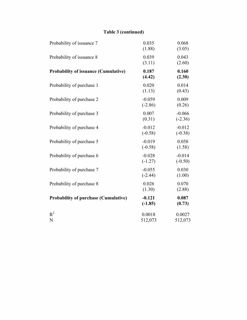
Table 3 (continued) Probability of issuance 7

0.035

0.068

(1.88) (3.05)


Probability of issuance (Cumulative) 0.187 0.160 (4.42) (2.30)

Probability of purchase 1 0.020 0.014 (1.13) (0.43)

Probability of purchase 2 -0.059 0.009 (-2.86) (0.26)

Probability of purchase 3 0.007 -0.066 (0.31) (-2.36)

Probability of purchase 4 -0.012 -0.012 (-0.58) (-0.38)


Probability of purchase 6 -0.028 -0.014 (-1.27) (-0.50)


Probability of purchase 8 0.026 0.070 (1.30) (2.88)

Probability of purchase (Cumulative) -0.121 0.087 (-1.85) (0.73)

R2 0.0018 0.0027 N 512,073 512,073

Table 4 Full Sample

( t-statistics in parentheses)

Unweighted Weighted

Mature dummy 1 0.006 0.001 (2.97) (0.09)

Mature dummy 2 -0.011 -0.024

(-2.23) (-3.80)

Mature dummy 3 0.002 -0.004 (0.89) (-0.69)

Mature dummy 4 -0.017 -0.003

(-4.82) (-0.63)

Mature dummy 5 -0.010 0.000 (-3.84) (-0.05)

Mature dummy 6 -0.006 0.008

(-1.86) (1.17)

Mature dummy 7 -0.031 -0.010 (-6.13) (-0.90)

Mature dummy 8 -0.020 -0.004

(-3.42) (-0.47)

Mature dummy (Cumulative) -0.086 -0.037 (-7.14) (-2.29)

R2 0.0007 0.0011 N 1,855,535 1,855,535

Table 5 Mature Sample, Iowa Futures--Dividend Interactions Only


Unweighted Weighted

∆Bush 0.035 -0.008 (4.77) (-0.68) ∆Bush x Dividend yield -0.413 -0.106

(-2.46) (-0.47)

R2 0.0007 0.0002 N 93,981 93,981

Table 6 Mature Sample, Iowa Futures--All Interactions


Unweighted Weighted

∆Bush 0.023 -0.046 (1.91) (-1.63) ∆Bush x Dividend yield -0.419 -0.079

(-2.62) (-0.37)

∆Bush x Probability of issuance 0.052 0.152 (1.68) (3.04)

∆Bush x Probability of purchase 0.005 0.106

(0.08) (1.06)

R2 0.0007 0.0011 N 93,981 93,981

Table 7 Full Sample, Iowa Futures (t-statistics in parentheses)

Unweighted Weighted

∆Bush 0.023 0.031 (3.86) (3.94) ∆Bush x Mature dummy 0.005 -0.039

(0.84) (-3.15)

R2 0.0002 0.0004 N 333,158 333,158

Table 8 Mature Sample--Dividend and Industry Average Dividend Interactions


Unweighted Weighted

Dividend yield 1 0.028 -0.080 (0.49) (-0.71)

Dividend yield 2 0.024 0.565 (0.30) (3.37)

Dividend yield 3 0.118 0.252 (1.18) (1.63)

Dividend yield 4 -0.199 -0.191 (-1.61) (-1.03)

Dividend yield 5 -0.125 0.064 (-1.66) (0.18)

Dividend yield 6 0.221 -0.095 (1.28) (-1.10)

Dividend yield 7 0.094 -0.157 (1.12) (-0.79)

Dividend yield 8 0.050 0.323 (0.40) (1.28)


Table 8 (continued) Industry average dividend yield 1 0.254 0.274

(4.26) (1.87)

Industry average dividend yield 2 0.068 -0.222 (0.58) (-0.96)

Industry average dividend yield 3 0.294 0.045 (2.29) (0.23)


Industry average dividend yield 5 -0.346 -0.150 (-3.18) (-0.49)

Industry average dividend yield 6 -0.330 -0.181 (-2.26) (-2.12)



Industry average dividend yield (Cumulative) 0.946 1.187 (2.54) (1.70)

R2 0.0017 0.0023 N 512,073 512,073

Table 3’

Mature Sample--All Interactions (t-statistics in parentheses)

3-Factor Model Institutional Ownership

Unweighted Weighted

Unweighted Weighted

Dividend yield 1 0.123 0.126 0.135 0.130 (2.71) (1.22) (2.89) (1.18)

Dividend yield 2 0.008 0.382 -0.033 0.364 (0.11) (2.17) (-0.42) (1.97)

Dividend yield 3 0.191 0.204 0.214 0.201 (2.05) (1.17) (1.89) (1.18)

Dividend yield 4 -0.099 0.183 -0.127 0.204 (-0.77) (1.03) (-1.04) (1.13)

Dividend yield 5 -0.161 0.174 -0.302 -0.001 (-2.19) (0.79) (-3.61) (-0.00)

Dividend yield 6 0.098 -0.240 0.070 -0.201 (0.63) (-3.73) (0.40) (-3.30)

Dividend yield 7 0.189 0.224 0.257 0.389 (2.24) (1.30) (2.40) (2.08)

Dividend yield 8 0.224 0.546 0.170 0.507 (1.49) (3.63) (1.27) (3.60)

Dividend yield (Cumulative) 0.573 1.600 0.385 1.594 (1.58) (2.65) (1.13) (2.74)

Probability of issuance 1 0.015 0.003 0.014 -3.47E-04 (1.34) (0.16) (1.26) (-0.02)

Probability of issuance 2 0.030 0.057 0.033 0.050 (1.94) (2.06) (2.24) (1.64)

Probability of issuance 3 0.020 -0.006 0.022 -0.010 (1.48) (-0.34) (1.55) (-0.54)

Probability of issuance 4 0.048 -0.007 0.053 0.002 (3.71) (-0.37) (4.02) (0.10)

Probability of issuance 5 0.007 -0.001 0.004 0.006 (0.34) (-0.06) (0.21) (0.34)

Probability of issuance 6 -0.009 -0.007 -0.004 0.003

(-0.73) (-0.62) (-0.33) (0.30)

Table 3’ (continued) Probability of issuance 7

0.031

0.058

0.038

0.066

(1.60) (2.41) (1.96) (3.05)

Probability of issuance 8 0.040 0.033 0.040 0.037 (3.01) (1.91) (3.15) (2.27)

Probability of issuance (Cumulative) 0.182 0.130 0.200 0.153 (4.33) (1.82) (4.69) (2.16)

Probability of purchase 1 0.020 0.016 0.022 0.011 (1.12) (0.48) (1.21) (0.31)

Probability of purchase 2 -0.068 0.014 -0.030 0.019 (-3.29) (0.44) (-1.51) (0.53)

Probability of purchase 3 -0.001 -0.063 0.015 -0.054 (-0.04) (-2.25) (0.67) (-1.83)

Probability of purchase 4 -0.002 -0.018 -0.009 -0.023 (-0.11) (-0.53) (-0.44) (-0.72)


Probability of purchase 6 -0.021 -0.023 -0.020 -0.021 (-0.96) (-0.75) (-0.94) (-0.70)


Probability of purchase 8 0.039 0.068 0.025 0.057 (1.92) (2.89) (1.31) (2.38)

Probability of purchase (Cumulative) -0.094 0.073 -0.047 0.069 (-1.41) (0.60) (-0.76) (0.59)

Institutional Ownership 1 -- -- -0.002 0.008 (-0.35) (0.60)

Institutional Ownership 2 -- -- -0.042 -0.025 (-4.11) (-1.25)

Institutional Ownership 3 -- -- -0.011 -0.028 (-1.48) (-2.38)



Table 3’ (continued)



Institutional Ownership 8 -- -- 0.006 0.033 (0.75) (3.40)

Institutional Ownership (Cumulative) -- -- -0.100 0.045 (-4.20) (1.08)

R2 0.0011 0.0026 0.0021 0.0031 N 512,073 512,073 503,792 503,792

Table 4’

Full Sample-3 Factor Model ( t-statistics in parentheses)

Unweighted Weighted

Mature dummy 1 0.006 0.001

(2.94) (0.09)

Mature dummy 2 -0.013 -0.028 (-2.74) (-4.77)

Mature dummy 3 -0.001 -0.009 (-0.32) (-1.56)

Mature dummy 4 -0.014 0.001 (-4.08) (0.27)

Mature dummy 5 -0.002 0.014 (-0.66) (2.47)

Mature dummy 6 -0.005 0.008 (-1.60) (1.20)

Mature dummy 7 -0.035 -0.019 (-6.47) (-1.75)

Mature dummy 8 -0.014 0.005 (-2.61) (0.59)

Mature dummy (Cumulative) -0.079 -0.028 (-6.59) (-1.77)

R2 0.0004 0.0010 N 1,855,535 1,855,535

Table 6’ Mature Sample, Iowa Futures--All Interactions


Unweighted Weighted

∆Bush 0.024 -0.040 (2.01) (-2.09)

∆Bush x Dividend yield -0.413 0.054 (-2.55) (0.21)

∆Bush x Probability of issuance 0.051 0.135 (1.68) (4.26)

∆Bush x Probability of purchase 0.005 0.088 (0.08) (1.11)

∆Bush x Bush Favor -0.021 -0.030 (-0.73) (-0.88)

∆Bush x Dem Favor 0.005 0.016 (-0.08) (0.23)

R2 0.0008 0.0012 N 93,981 93,981

Table 7’ Full Sample, Iowa Futures (t-statistics in parentheses)

Unweighted Weighted

∆Bush 0.023 0.031 (3.82) (3.59)

∆Bush x Mature dummy 0.006 -0.036 (0.89) (-2.77)

∆Bush x Bush Favor -0.027 -0.024 (-1.26) (-0.81)

∆Bush x Dem Favor 0.059 0.056 (1.54) (1.67)

R2 0.0002 0.0001 N 333,158 333,158

Figure 1. Investment and Transition for Immature Firms

0

0.1

0.2

0.3

0.4

0.5

0.6

0 5 10 15 20 25 30

Period

Inve

stm

ent

0

0.2

0.4

0.6

0.8

1

1.2

q*

q* (θ = .1)

q* (θ = .3)

Investment (θ = .3)

Investment (θ = .1)

the 2003 dividend tax cuts and the value of the firm 2003 dividend tax cuts and the value of the...

Documents