texture analysis of sar sea ice imagery using gray level

University of Nebraska - Lincoln University of Nebraska - Lincoln

DigitalCommons@University of Nebraska - Lincoln DigitalCommons@University of Nebraska - Lincoln

CSE Journal Articles Computer Science and Engineering, Department of

3-1999

Texture Analysis of SAR Sea Ice Imagery Using Gray Level Co-Texture Analysis of SAR Sea Ice Imagery Using Gray Level Co-

Occurrence Matrices Occurrence Matrices

Leen-Kiat Soh University of Nebraska, [email protected]

Costas Tsatsoulis University of Kansas

Follow this and additional works at: https://digitalcommons.unl.edu/csearticles

Part of the Computer Sciences Commons

Soh, Leen-Kiat and Tsatsoulis, Costas, "Texture Analysis of SAR Sea Ice Imagery Using Gray Level Co-Occurrence Matrices" (1999). CSE Journal Articles. 47. https://digitalcommons.unl.edu/csearticles/47

This Article is brought to you for free and open access by the Computer Science and Engineering, Department of at DigitalCommons@University of Nebraska - Lincoln. It has been accepted for inclusion in CSE Journal Articles by an authorized administrator of DigitalCommons@University of Nebraska - Lincoln.

https://digitalcommons.unl.edu/

https://digitalcommons.unl.edu/csearticles

https://digitalcommons.unl.edu/computerscienceandengineering

https://digitalcommons.unl.edu/computerscienceandengineering

https://digitalcommons.unl.edu/csearticles?utm_source=digitalcommons.unl.edu%2Fcsearticles%2F47&utm_medium=PDF&utm_campaign=PDFCoverPages

http://network.bepress.com/hgg/discipline/142?utm_source=digitalcommons.unl.edu%2Fcsearticles%2F47&utm_medium=PDF&utm_campaign=PDFCoverPages

https://digitalcommons.unl.edu/csearticles/47?utm_source=digitalcommons.unl.edu%2Fcsearticles%2F47&utm_medium=PDF&utm_campaign=PDFCoverPages

780 IEEE TRANSACTIONS ON GEOSCIENCE AND REMOTE SENSING, VOL. 37, NO. 2, MARCH 1999

Texture Analysis of SAR Sea Ice ImageryUsing Gray Level Co-Occurrence Matrices

Leen-Kiat Soh,Member, IEEE, and Costas Tsatsoulis,Senior Member, IEEE

Abstract—This paper presents a preliminary study for mappingsea ice patterns (texture) with 100-m ERS-1 synthetic apertureradar (SAR) imagery. We used gray-level co-occurrence ma-trices (GLCM) to quantitatively evaluate textural parametersand representations and to determine which parameter valuesand representations are best for mapping sea ice texture. Weconducted experiments on the quantization levels of the imageand the displacement and orientation values of the GLCM byexamining the effects textural descriptors such as entropy have inthe representation of different sea ice textures. We showed that acomplete gray-level representation of the image is not necessaryfor texture mapping, an eight-level quantization representationis undesirable for textural representation, and the displacementfactor in texture measurements is more important than orien-tation. In addition, we developed three GLCM implementationsand evaluated them by a supervised Bayesian classifier on sea icetextural contexts. This experiment concludes that the best GLCMimplementation in representing sea ice texture is one that utilizesa range of displacement values such that both microtexturesand macrotextures of sea ice can be adequately captured. Thesefindings define the quantization, displacement, and orientationvalues that are the best for SAR sea ice texture analysis usingGLCM.

Index Terms—Co-occurrence matrix, SAR, sea ice, texture.

I. INTRODUCTION

I N THIS paper, we present a set of experiments on tex-tural parameters and representations and a quantitative

evaluation of these experiments, which shows which texturalparameter values and texture representations are best fordescribing sea ice in synthetic aperture radar (SAR) imagery.We selected seven different sea ice textural contexts, i.e., seaice texture types, and used them as our test set. These texturalcontexts have no definitive, intrinsic geophysical significanceand were so selected because they werevisually separable bya human, without being too different as to make the separationtrivial. We computed the texture matrix representations ofthese sample contexts and used a supervised Bayesian clas-sifier to evaluate how well the texture matrices could describeand recognize the textural contexts.

The texture matrix used was the gray-level co-occurrencematrix (GLCM). In designing the GLCM for texture repre-sentation, there are three fundamental parameters that must

Manuscript received June 5, 1997; revised March 11, 1998. This work wassupported in part by the Naval Research Laboratory Award N00014-95-C-6038 and by the NSF Grant CISE-CDA-9401021.

The authors are with the Information and Telecommunication Technol-ogy Center (ITTC), Department of Electrical Engineering and ComputerScience, The University of Kansas, Lawrence, KS 66045 USA (e-mail:[email protected]).

Publisher Item Identifier S 0196-2892(99)01172-9.

be defined: the quantization levels of the image and thedisplacement and orientation values of the measurements.We performed a set of experiments in which we systemati-cally varied these parameters and studied how the variationsaffected GLCM standard texture descriptors for SAR seaice images. From these experiments, we concluded whichquantization levels and displacement and orientation valuesare best for representing sea ice texture in SAR. We developedand evaluated three different implementations of GLCM, themean displacement and mean orientation (MDMO) matrix,the -optimal displacement and mean orientation (ODMO)matrix, and the -optimal displacement and -optimal ori-entation (ODOO) matrix. The implementations were evaluatedas to their ability to separate between sea ice texture contexts.Based on these experiments, we concluded which texturematrix representation is best at separating sea ice texture typesin SAR imagery.

The ability to represent sea ice texture contexts well, i.e., ina way that allows classification and separation of the contexts,is extremely significant in sea ice analysis, classification, anddescription. Statistical texture analysis is important in SAR seaice imagery research since it allows better representation andsegmentation of sea ice regions, compared to analysis based onintrinsic gray levels only. It has been shown that the inclusionof texture as a descriptor can improve the classification ofsea ice and the description of sea ice deformations [38], [56],[63]. Some work has attempted to identify which texturalmeasurements provide better descriptors for sea ice [65],but no work has provided a comprehensive experiment oftextural parameters and representations with an evaluation ofthe quality of the representation based on quantifiable metrics.Our work is the first one to evaluate all possible textural rep-resentation parameters and to make specific recommendationsabout the representation of sea ice texture in SAR imagery.

II. BACKGROUND ON GLCM

The definition of GLCM’s is as follows [35]. Suppose animage to be analyzed is rectangular and has columnsand rows. Suppose that the gray level appearing at eachpixel is quantized to levels. Letbe the columns, be the rows, and

be the set of quantizedgray levels. The set is the set of pixels of theimage ordered by their row–column designations. The image

can be represented as a function that assigns some graylevel in to each pixel or pair of coordinates in

; . The texture-context information is

0196–2892/99$10.00 1999 IEEE

Digital Object Identifier: 10.1109/36.752194

SOH AND TSATSOULIS: TEXTURE ANALYSIS OF SAR SEA ICE IMAGERY 781

specified by the matrix of relative frequencies with twoneighboring pixels separated by distanceoccur on theimage, one with gray level and the other with gray level. Such matrices of gray-level co-occurrence frequencies are

a function of the angular relationship and distance betweenthe neighboring pixels. Formally, for angles quantized to 45intervals, the unnormalized frequencies are defined as shownin the equations at the bottom of hte page wheredenotesthe number of elements in the set.

We used ten textural features in our study. The followingequations define these features. Let be the th entryin a normalized GLCM. The mean and standard deviations forthe rows and columns of the matrix are

The features are as follows.

1) Energy:

2) Contrast:

3) Correlation:

4) Homogeneity:

5) Entropy:

6) Autocorrelation:

7) Dissimilarity:

8) Cluster Shade:

9) Cluster Prominence:

10) Maximum Probability:

MAX

Note that energy is also popularly known as angular secondmoment [30]. The two cluster parameters were introducedin [19] to emulate human perceptual behavior. Maximumprobability was discussed in [34]. Energy, contrast, correlation,homogeneity, entropy, autocorrelation, and dissimilarity wereformulated in [35].

Zucker and Terzopoulos [70] proposed an algorithm forselecting GLCM for texture classification using a test.The notion of the structure capturable by GLCM is relatedto the confidence regarding the variablegiven the variable

, and vice versa. The null hypothesis of the test that thesetwo variables are independent is in the form of

where is the probability corresponding to theth rowand is the probability corresponding to theth column.From the derivation presented in [70], the authors arrived at acomputationally efficient expression for the test

where , , and

. The optimal matrix is the matrix that

or

or


yields the highest value of . As a result, we can determinethe displacement and orientation parameters for a certaintexture class by simply examining the optimal GLCM. Theauthors applied the test on several Brodatz [9] patterns. Itwas observed that for values of displacement and orientationthat captured texture structure well, the correspondingvalues were high, supporting the validity of the test. As wehave mentioned, we used this test in our experiments.

A. Applications

Haralick et al. [35] illustrated the applications of texturalfeatures based on GLCM on three different kinds of im-age data: photomicrographs of different kinds of sandstones[60], panchromatic aerial photographs of land-use categories,and earth resources technology satellite (ERTS) multispectralimagery containing land-used categories. Krugeret al. [45]employed GLCM to capture visual texture-context informa-tion in an interrib space of X-ray imagery. Chien and Fu[13] computed the average and variance of five augmentedGLCM textural features to identify texture changes of X-raypictures to detect venus hypertension in lung field. Davisetal. [21] used generalized GLCM to impose spatial constraints.Shanmuganet al. [61] used segments of digitally correlatedSEASAT-A SAR imagery in their attempt to classify radarimages based on GLCM textural features. Connerset al. [19]used texture to segment a high-resolution black and whiteimage of an urban area. Gotlieb and Kreyszig [31] derived ageneral model for analysis and interpretation of experimentalresults in texture analysis when raw and composite texturalfeatures were used. Barber and LeDrew [5] reported univariateand multivariate analyses in describing the separability of SARsea ice feature space based on GLCM, tested on a STAR-1SAR image. Sali and Wolfson [59] used a clustering algorithmbased on a generalized Lloyd algorithm and an iterativeregion merging process based on the phagocytes heuristic toclassify SPOT satellite images using GLCM-based texturalfeatures. Kushwahaet al. [47] used GLCM to classify IRSLISS-II sensor data on forest analysis in northeastern India.Franklin and Peddle [26] improved classification of SPOTHRV imagery for a moderate-relief environment in easternCanada from 51.1 (spectral alone) to 86.7% (spectral dataplus GLCM features). The authors also conducted textureanalysis of land systems from Landsat MSS data [25]. Baraldiand Parmiggiani [3] used GLCM to classify SPOT urbanareas. Chen and Pavlidis [11] combined a GLCM and a split-and-merge algorithm to segment images in a multiresolutionapproach. Trivediet al. [66] presented a module that wasable to detect fixed orientation objects from a wide varietyof backgrounds. They used a supervised parametric methodbased on a distribution to guide a forward sequential searchalgorithm in the object detection phase. Kovalev and Petrou[44] used multidimensional GLCM to perform classificationof various images of CT brain scans, several types of mi-croscope images, and photographs of signatures. Haddon andBoyce [32], [33] proposed one interesting application of co-occurrence matrices in which the matrices were used to detectedges and estimate optic flow field. Beaucheminet al. [6]

Fig. 1. Image of mostly multiyear ice with heavy ridging and deformation,categorized as Web. Each sample site is 64� 64, or 40.96 km2. ESA.

used GLCM to design an adaptive speckle-removal filter andan edge detector.

III. SAR SEA ICE IMAGERY AND TEXTURAL CONTEXTS

We analyzed over 2000 ERS-1 SAR low-resolution imagesof the Bering, the Beaufort, and the Chukchi seas for everymonth of the year and compiled seven classes of SAR sea icetextural contexts based on human visual inspection. Note thatthese seven types of textural contexts do not fully describe allSAR sea ice imagery, and they certainly do not correspondspecifically to all ice types. These classes were selected sothat we could compare different implementations of GLCMin terms of their classification power and demonstrate thefeasibility of GLCM-based textural contexts in differentiatingsea ice imagery.

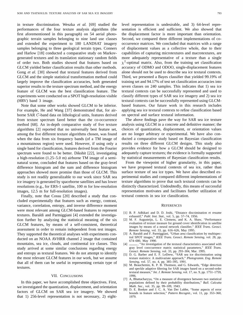
Class 1—Web:Fig. 1 shows an image taken onMarch 27, 1992, at 73.466N and 156.19 E. The imageconsists of mostly multiyear ice with heavy ridging anddeformation. The web-like structure that these ridges ordeformations build with each other characterizes this typeof images.

Class 2—3-D: Fig. 2 shows an image taken on February7, 1993, at 58.54 N and 163.63 W. The image consists ofcrushing floes creating extreme deformations in the marginalice zone (MIZ). Boundaries of floes have been roughened suchthat they give high backscatter return. These thick enclosingstructures portray a three-dimensional (3-D) perceptual effectthat characterizes this type of image.

Class 3—Fractal: Fig. 3 shows an image taken on Septem-ber 8, 1993, at 77.35N and 145.79 W. The image consistsof mostly new ice and melt ponds. This phenomenon occursat the end of the summer melt season when ice floes havebeen broken up, brushed, and rubbled. Boundaries of floes


Fig. 2. Image of crushing floes with extreme deformations at MIZ, catego-rized as 3-D. Each sample site is 64� 64, or 40.96 km2. ESA.

Fig. 3. Image of mostly new ice and melt ponds, categorized as fractal. Eachsample site is 64� 64, or 40.96 km2. ESA.

look foamy and wiggly fractal, and it is this property thatcharacterizes this type of images.

Class 4—Pebble-Like:Fig. 4 shows an image taken on July12, 1993, at 72.26N and 160.47 W, showing the start ofthe summer melt season. Multiyear ice can be seen as littleround features; younger ice as quite homogeneous but grainypatches. Pebbles of ice floes are embedded in about-to-meltyounger ice formations. The pebbles characterize this type ofimages.

Fig. 4. Image of thawing multiyear (small circular structures) and first-yearice, categorized as pebble-like. Each sample site is 64� 64, or 40.96 km2. ESA.

Fig. 5. Image of highly undeformed ice features, categorized as smooth.Each sample site is 64� 64, or 40.96 km2. ESA.

Class 5—Smooth:Fig. 5 shows an image taken on Febru-ary 1, 1994 at 72.06N and 176.39 W. This image showsvery smooth multiyear and first-year ice with bright refrozenleads cutting across the region. As we can see, dark patches(probably multiyear) and bright sheets (probably young ice)are extremely homogeneous and uniform. These are consideredas highly undeformed ice features, characterizing this type ofimages.


Fig. 6. Image of regions with substantial size and of two highly contrastingintensities, categorized as high-contrast. Each sample site is 64� 64, or40.96 km2. ESA.

Class 6—High Contrast:Fig. 6 shows an image taken onNovember 17, 1993, at 72.27N and 154.75 W. This imageshows on the one hand large dark multiyear ice floes and on theother hand, large refrozen young first-year ice and thin pancakeice. This combination of phenomena tells us that the floes hadbeen mobile to create water lodgings and stationary enough forpancake or young ice to form. These regions with substantialsize and of two highly contrasting intensities characterize thistype of images.

Class 7—Packed:Fig. 7 shows an image taken on March17, 1992, at 72.85N and 143.83 W. This image shows apiece of packed multiyear ice broken by large leads. Thereare refrozen leads developing in some areas, and open waterregions are rare. These multiyear ice conglomerates are slightlyridged but mostly undeformed. This context is frequentlyobserved around high latitude regions or in the middle periodof winter since floes are frozen and relatively immobile.

IV. QUANTIZATION , DISPLACEMENT,AND ORIENTATION FACTORS ON GLCM

There are several important parameters to consider whendesigning a GLCM, as follows: 1) the region size, 2) thequantization levels, , 3) the displacement value, and 4) theorientation value . The region size gives the dimensions ofthe region of which GLCM is computed. In Haverkampet al.[36], the region sizes of 32 32 and 64 64 were used toperform dynamic local thresholding on SAR sea ice imagerysuccessfully. In order to capture sea ice textural contexts, weprefer the larger region size and set it to 6464 during ourexperiments with GLCM. In the following, we will examinethe quantization and displacement factors directly and theorientation factor indirectly in Section V.

Fig. 7. Image of slightly ridged but mostly undeformed multiyear ice, andwith good three-class separation (MY, FY, and OW/NI), categorized aspacked. Each sample site is 64� 64, or 40.96 km2. ESA.

The approach of our experiment is as follows. For quanti-zation, we compute a set of quantized images of each samplesite. Then, a second-order Euclidean distance measure betweeneach successive pair of the quantized images is computedbased on the second-order statistics of GLCM of the quantizedimages. The visual observation of the measurements serves asthe basis for our conclusions regarding the quantization factors.For displacement, once again, we compute a set of quantizedimages of each sample site. Then we compute various second-order GLCM statistics of the quantized images using a set ofdisplacement values. We visually inspect the curves generatedby plotting the statistics against the displacement values foreach sample site and draw conclusions from the observation.Finally, for orientation, we design three implementations ofGLCM and by comparing the classification powers of thedesign, we are able to draw some conclusions regarding theorientation factors for sea ice textural contexts.

A. Quantization

The number of gray levels is an important factor in thecomputation of GLCM. The decision that we have to makeis how many levels are needed to represent a set of texturessuccessfully. The more levels included in the computation,the more accurate the extracted textural information, with,of course, a subsequent increase in computation costs sincethe quantization scheme smoothes an image and thus reducesnoise-induced effects to some degree. We assume that theinformation gain in noise-effect reduction does not compensatethe loss of information as a result of quantization. There arethree major quantization schemes: 1) uniform quantization, 2)Gaussian quantization, and 3) equal probability quantization.The uniform quantization scheme is the simplest, in which


gray levels are quantized into separate bins with uniformtolerance limits or spaces with no regard to the gray-leveldistribution of the image. This technique is not always prefer-able. For example, if a range of gray levels occurs morefrequently than others, we might desire to finely quantizethat particular range. The Gaussian quantization techniqueis one such scheme. According to this scheme, the gray-level distribution of the original image is assumed to behavenormally. Each quantization bin has the same area under thecurve and thus different space smaller spaces in the middle ofthe distribution and larger spaces at the tails of the distribution.The equal probability quantization [35] scheme has also beenused such that each bin has a similar probability, and it hasbeen shown to retain an accurate representation of the originalpicture in terms of textural features based on GLCM [17].The Gaussian quantization scheme assumes a Gaussian gray-level distribution, which is not always true for SAR sea iceimagery. Equal probability quantization normalizes differentimage samples so that a bright feature and a dark feature, giventhe same texture, would have the same co-occurrence matrix,which is undesirable since the backscatter of sea ice types isa key parameter in sea ice analysis. Thus, in our experiment,we have focused on the uniform quantization scheme.

We extracted sample sites, each 6464, from 18 imageswith different textural contexts in this experiment. We deviseda test using six textural features (energy, contrast, correlation,entropy, autocorrelation, and homogeneity) and six differentuniform quantization schemes: 8, 16, 32, 64, 128, and 256levels. We set displacement to one and orientations to 0, 45,90, and 135. Taking the average of the orientations for eachimage sample yields a 6 6 matrix. Each entry of this texturalvector is defined as , where , ,and . is the index of the textural features,is the index of the quantization schemes (such that scheme

has quantization levels), and denotes thesite label ( total number of sample sites). The differentvalues of the quantization are evaluated by five measures basedon Euclidean distance along each textural feature betweeneach pair of sample sites. Note that the objective of thefollowing Euclidean distance measures is to provide a visualpresentation of the trend between the differences between eachsuccessive pair of quantization schemes. These measures weredesigned to capture such differences without assuming thedistribution or any prior knowledge of the samples. Therefore,statistical distance measures (that are also computationallymore complicated), such as Mahalanobis [51], Kolmogorov[1], Bhattacharyya [7], Bayesian distance [8], Chernoff [12],Matsusita [52], and divergence [40], [46], and those utilizedin pattern recognition [50], [57], have not been used in ourexperiment.

The first measure is the normalized first-order differentiation

is the image label.

This value measures the normalized difference between twosample sites from the same image in terms of a particulartextural feature. The collective results for each sample pair isa 6 6 matrix. Observing this matrix gives us an idea how

the degree of dissimilarity between two samples varies withthe number of quantization levels.

The second measure is the neighbored second-order autod-ifferentiation

and

This value measures the average absolute difference betweenthe normalized first-order differentiation between two neigh-boring quantized schemes, taken over all sample pairs ofthe same image. This matrix tells us whether there existsa systematic relationship between two neighboring quantizedschemes.

The third measure is the biased second-order autodifferen-tiation

and

This value measures the average absolute difference betweenthe normalized first-order differentiation between a -quantization and the 256-quantization (or the original image,in our case) scheme, where , taken over allsample pairs of the same image. This matrix tells us whichquantization scheme best imitates the result of 256-levelquantization scheme.

The fourth measure is the neighbored second-order crossdifferentiation

and

Note that is the total number of sample sites in the imagewith the label . This value measures the average absolutedifference between the normalized first-order differentiationbetween two neighboring quantization schemes, taken over allsample pairs of two different images.

The fifth measure is the biased second-order cross differ-entiation

and

This value measures the average absolute difference betweenthe normalized first-order differentiation between a -quantization and the 256-quantization (or the original image,in our case) scheme, where , taken over all samplepairs of two different images.

Fig. 8 shows one graphical example of the normalized first-order differentiation matrix. Note that this graph shows thedifferences between two sample sites in terms of six texturalfeatures when the sites are quantized with eight levels, 16levels, and so on, up to 256 levels (the original). We can seethat for the eight-level quantization scheme, the differentiation


Fig. 8. Example of the first-order differentiation of textural feature measure-ments versus quantization schemes. There is no noticeable trend of how degreeof similarity between two samples varies with the number of quantizationlevels. Note: quantization scheme 1 denotes eight-level quantization; 2 denotes16-level, and so on. Filled triangle: entropy, filled square: autocorrelation,filled diamond: contrast, filled circle: correlation, square: homogeneity, andtriangle: energy.

values are noticeably different from others. Also, we can seethat, for other quantization levels, the differences betweenthe two sample sites are very similar. This hints that if ourobjective is to distinguish between two sea ice contexts, thenumber of quantization levels (excluding eight) do not matter.To analyze whether the textures can be used to represent seaice contexts, we turn to second-order differentiation values.Fig. 9 shows some examples of our neighbored second-orderdifferentiation: (a) , (b) where images and areof the same context, and (c) where images andare of different contexts. Note that only four textural featuresare shown so the scale of the texture value can be displayedadequately for view. Generally, the distance between featuresof two neighboring quantization schemes decreases as morequantization levels are involved for all .This indicates that, if we assume the original image to beaccurate, information loss to quantization is gradual: morewhen the number of quantization levels is smaller and viceversa. From another perspective, if we choose a high enoughnumber of quantization levels, we will be able to preserveenough information found in the image. In addition, weobserve that such distance is the smallest for the samplesfrom the same image and the largest for two samples fromdifferent textural contexts

. This indicates that not only GLCMcan recognize different contexts, whether they are from thesame or different images, but it can do it for a differentnumber of quantization levels. Fig. 10 shows some examplesof biased second-order differentiation measures: (a), (b)

where images and are of the same context, and(c) where images and are of different contexts,respectively. Generally, we can derive similar observations, asdiscussed in the neighbored case , for all ,

. So,while the representative power of the GLCM deteriorates withincreased quantization, the discriminative power of GLCM

(a) (b) (c)

Fig. 9. Example of (a) neighbored second-order autodifferentiation, (b)neighbored second-order cross differentiation (within same context), and(c) neighbored second-order cross differentiation (with different contexts).All plots are in log scale. Difference between two neighboring featuremeasurements is generally smaller as the number of quantization levelsincreases. Note: quantization scheme 1 denotes eight-level quantization; 2denotes 16-level, and so on. Graphs show energy (filled square), contrast(square), autocorrelation (filled diamond), and homogeneity (diamond).

does not, if used in characterizing and recognizing sea icecontexts.

Several conclusions have been drawn from the experiments,as follows.

1) There is no noticeable trend to indicate that the degreeof dissimilarity between two samples varies with thenumber of quantization levels. But there are noticeabledifferences, more random than systematic.

2) There is a noticeable trend that shows diminishingdifference when comparing results of a pair of largernumbers of quantization levels. This indicates that theGLCM-based results are more consistent when usinga higher number of quantization levels. This disagreeswith the findings of [53]. The probable cause of thisdisagreement lies at the number of quantization levelsanalyzed: in [53], the authors usedonly the 16- and32-level quantization schemes and found their texturalfeatures to be similar; and we compared quantizationlevels to the original image.

3) Degree of dissimilarity is the smallest when the samplesare of the same image, small when the samples are oftwo images of the same context, and the largest whenthe samples are of two images of different contexts. Thisindicates that the GLCM can be utilized to differen-tiate two different contexts and recognize two similarcontexts.


(a) (b) (c)

Fig. 10. Example of (a) biased second-order autodifferentiation, (b) biasedsecond-order cross differentiation (within same context), and (c) biasedsecond-order cross differentiation (with different contexts). All plots are in logscale. Second-order differentiation values between other feature measurementsand those of 256-level quantization is generally smaller as the number ofquantization levels increases. Note: quantization scheme 1 denotes eight-levelquantization; 2 denotes 16-level, and so on. Graphs show energy (filledsquare), contrast (square), autocorrelation (filled diamond), and homogeneity(diamond).

4) As expected, as the number of quantization levels in-creases, features imitate those of the original quantiza-tion more closely. This trend is clearly noticeable for allsample pairs.

5) The eight-level quantization scheme is consistently andnoticeably different from other schemes. Thus, it shouldnot be used.

B. Displacement

The displacement parameter is important in the com-putation of GLCM. Applying a large displacement value toa fine texture would yield a co-occurrence matrix that doesnot capture the textural information, and vice versa. Chenet al. [10] used and found thatoverall classification accuracies with wereessentially equivalent in differentiating cloud types. However,for higher displacement values, the authors found that theclassification accuracies decreased. They also concluded thatthe classification result was best when using features frommatrices of . This indicates that single-displacementfeatures might not be sufficient to represent textures. Anotherstudy [22] showed that a displacement value equal to the sizeof the texture element would tend to improve the classificationresult with texture features. For our experiment, we used

. We used 32 as our upper limit of range as

Fig. 11. Graph of an example of normalized energy for all displacementcurves across all quantization schemes.

Fig. 12. Graph of an example of normalized contrast for all displacementcurves across all quantization schemes.

it was half the region size of each sample. To better comparethe texture values across different quantization schemes, wenormalized each series by dividing it by its maximum value.Figs. 11–18 show the graphs of normalized texture valuesversus quantization schemes. In general, we can see thatacross different quantization schemes, displacement curvespreserve nicely. In particular, for contrast and dissimilarity, alldisplacement curves, after normalization, are almost identical.This indicates that quantization does not affect the two texturalfeatures. For energy, correlation, homogeneity, entropy, andautocorrelation, the behaviors of the curves are similar in termsof locations of upward and downward slopes along the curves.The differences are in the degree of these slopes, which areprobably caused by reduced resolutions in the reduction ofquantization levels. This indicates that, although the loss ofinformation is visible, the inherent structures of relationshipsamong pixels for these textural features are still intact and


Fig. 13. Graph of an example of normalized correlation for all displacementcurves across all quantization schemes.

Fig. 14. Graph of an example of normalized homogeneity for all displace-ment curves across all quantization schemes.

can be captured and represented with GLCM. For maximumprobability, peaks and valleys are more prominent as theresolution of the sample site increases. Note that the definitionof max probability is MAX . Unlike others, itis not a function of an aggregate of . Thus, the valueof this parameter is more volatile and susceptible to loss ofinformation due to quantization. As we can see from Fig. 18,peaks and valleys have been lost, and when the number ofquantization levels reduces to eight (the thin solid line), thedisplacement curve becomes the smoothest. In general, alldisplacement curves still follow a similar trend.

Several conclusions have been drawn from this experiment,as follows.

1) Across quantization schemes, each textural curve pre-serves nicely. This hints that the number of quantizationlevels can be arbitrarily chosen as long as a range of

Fig. 15. Graph of an example of normalized entropy for all displacementcurves across all quantization schemes.

Fig. 16. Graph of an example of normalized autocorrelation for all displace-ment curves across all quantization schemes.

displacement values are used in computing the GLCM,and thus, we eliminate the need for 128-level and 256-level schemes, which are computationally very costly.In [10], the authors showed that classification of cloudfields was still successful even with the highly quantizedversion of GLCM features. Compared to that finding, ourobservation is a more restricted case.

2) Instead of a multiresolution approach that coordinatesdifferent quantization schemes, it is sufficient to use onequantization scheme with a range of displacement valuessince the dynamics of curves of different number ofquantization levels are similar.

3) There is no hint on determininga priori a generaldisplacement value for all samples in which each sampleapproaches an asymptotic plateau. This indicates that itis necessary to compute matrices of different displace-ment values to obtain accurate textural features (even


Fig. 17. Graph of an example of normalized dissimilarity for all displace-ment curves across all quantization schemes.

Fig. 18. Graph of an example of normalized maximum probability for alldisplacement curves across all quantization schemes.

though it is not necessary to use all such matrices).Asingle displacement value for GLCM to represent sea icetextural contexts is not advisable.

4) Averaging features over a range of displacement valuesmight be used to obtain a reliable and economical repre-sentation, especially for asymptotic curves. For example,each sample has four features, eight displacement values,and four quantization schemes, yielding a total of 128values. The averaged version has only 16 values.

C. Orientation

The orientation parameter is relatively less importantcompared to other factors in co-occurrence matrices. Someauthors used the average and range, some used certain seriesof orientations; for example, , 75, 90, 109, and 165to accommodate man-made urban structures [19], range and

average of , 45, 90, and 135 [35], average of two by126 apart, average of three by 66apart, and average of fourby 37 apart [56] average of , 45, 90, and 135 [38],average, variance and range of , 45, 90, and 135[45],and prespecified orientation for each image [66].

For SAR sea ice imagery, there are no systematic patternsbased on orientation. Ice features rotate and position them-selves in all possible orientations. Therefore, we argue thatthe orientation factor is not important in SAR sea ice research.We used , 45, 90, and 135 for they cover efficientlyall directions of SAR sea ice imagery, as we shall show inthe next section.

V. THREE CO-OCCURRENCEMATRICES

FOR SEA ICE TEXTURAL CONTEXT

In this experiment, we designed and compared three differ-ent GLCM implementations by subjecting them to training andtesting of a database of sea ice sample sites. We evaluated theclassification powers of the designs based on a Bayes classifier.Based on the classification accuracies, we were able to derivethe importance of the orientation factor and an effective wayof utilizing displacement values.

The first design is the MDMO matrix. Feature measures ofthe matrices of the four orientations of 0, 45, 90, and 135areaveraged, and further averaged over the displacement range.Note that the average over the displacement range is our choiceof aggregating feature measures of different displacementvalues. Other approaches, such as curve approximation orparametric polynomial modeling, can be used to describe thedisplacement curves for a more complete representation. Notethat other higher level treatment of features of different dis-placement values is also possible, such as principal componentanalysis of the eigenvector of different features.

Let the set of all displacement values be and the setof all orientations be ; let be the co-occurrencematrix computed with displacementand orientation ; andlet be the feature computed with displacementand orientation . Formally

where is the number of members in the set. TheMDMO implementation assumes that every matrix of specificdisplacement and orientation is partially and cumulativelyrepresentative for the sample.

The second GLCM is the -ODMO matrix. values ofall four matrices of different orientations are calculated andaveraged for each displacement, and the matrix accumulatingthe most value is the optimal matrix. Let bethe of . Formally


The ODMO implementation assumes that only the matrixwhose value is the highest with a specific displacementvalue is truly and sufficiently representative for the sample,with no regard to selective orientation.

The third GLCM is the -optimal displacement and ODOOmatrix. Formally

The ODOO implementation assumes that the matrix whosevalue is the highest with specific displacement and orientationis truly and sufficiently representative for the sample.

We elected to use the ability of a GLCM to classify betweendifferent textures as a metric of its efficacy. Classification wasperformed using a Bayesian supervised classifier. Using allten features outlined in Section II, we have for each samplethree vectors of ten entries , andgrouped into three groups for all samples, ,and , respectively. For each group of data, samplesof seven textural contexts, for , are used totrain the Bayes classifier. For each context, we calculatedits discriminant function

where is the unknown sample vector of the calculatedmean vector for and is the calculated covariance for

. The classifier assigns a sampleto if

for all

Note that, in all of the experiments that follow, we usedthe uniform 64-level quantization scheme. This number ofquantization levels was chosen since, used over a range ofdisplacement values, it preserves textural information well andit does not incur as much computational load as other higherlevel quantization schemes.

A. Experimental Evaluation of GLCM’s

In our first experiment, we used ten features, 228 samples,18 images, and six contexts. The resubstitution classificationor training set classification accuracies of the MDMO, ODMO,and ODOO implementations are tabulated in Table I. Thenumbers represent the accuracy by which a specific GLCM canclassify a sample into one of six contexts. Consequently, it is ametric of representational quality. From the table, we observethat the MDMO implementation has the best classificationresults on the training set with overall accuracy above 90%.

After generating features for all samples, we noticed thatthe cluster shade and cluster prominence measurements showhigher range and range/mean (normalized range) values thanthe other measurements (Table II). This is probably due to thethird and fourth order of moments used in the computation,

TABLE ICLASSIFICATION ACCURACY AFTER SUPERVISED TRAINING, BASED ON THE

TRAINING DATA SETS. MDMO’s CLASSIFICATION ACCURACY IS BETTER THAN

THE OTHER TWO FOR ALL CLASSES, EXCEPT FORCLASS 1. ALL THREE

IMPLEMENTATIONS FAILED TO CLASSIFY CLASS 2. TEN FEATURES WERE USED

TABLE IIFEATURES FOR ACLASS 1 SAMPLE. NOTE THAT BOTH CLUSTER SHADE AND

PROMINENCE HAVE THE HIGHEST RANGE AND RANGE/MEAN VALUES. THIS

CHARACTERISTIC CREATES A PROBLEM FOR OUR BAYESIAN CLASSIFIER

TABLE IIIRESUBSTITUTION CLASSIFICATION ACCURACY AFTER SUPERVISED

TRAINING, BASED ONLY ON THE DATA SETS. MDMO’sCLASSIFICATION ACURACY WAS IMPROVED WHEN CLUSTER SHADE

AND PROMINENCE WERE EXCLUDED FROM THE FEATURE SET

respectively. Using higher order moments amplifies the surfaceof a cluster. If the cluster was roughly homogeneous, theresulting feature value would be consistent and occupy acompact range. As we can see from Table II, both normalizedranges are higher for cluster shade and prominence. This hintsthat the quantized images do not possess good cluster-typecharacteristics. We conducted an experiment to compare theclassification results between MDMO with all ten featuresand MDMO with eight features, excluding cluster shade andprominence. The results are shown in Table III. Overall, theexclusion of cluster shade and prominence improved ourclassification accuracy. Class 2 classification accuracy wasimproved from 16.67 to 100.00%. As a result, we believe thatthe cluster-type features (cluster shade and cluster prominence)tend to extenuate the clustering characteristic of samples anddominate classification resulting in large errors.


TABLE IVRESUBSITUTION CLASSIFICATION ACCURACY AFTER SUPERVISED TRAINING,

BASED ONLY ON THE DATA SETS. MDMO’s CLASSIFICATION ACURACY

IS BETTER THAN THE OTHER TWO FOR ALL CLASSES. EIGHT

FEATURES WERE USED. SEVEN CONTEXTS WERE REPRESENTED

TABLE VCONFUSION MATRICES. THE ROWS DENOTE THE ACTUAL CLASS OF

THE SAMPLE SITES, AND THE COLUMNS DENOTE THE CLASS FOUND

BY THE CLASSIFIER. (a) MDMO WITH TEN FEATURES. (b) ODOOWITH EIGHT FEATURES. (c) MDMO WITH EIGHT FEATURES.

(d) MDMO WITH EIGHT FEATURES. A PERFECT CLASSIFIER WOULD

HAVE NONZERO ENTRIES ONLY IN THE DIAGONAL OF THE MATRIX

(a) (b)

(c) (d)

B. Confusion Tables

We also conducted a test to see how our implementationsof the GLCM’s respond to different context classes throughthe use of confusion tables. We used eight features, 240samples, 19 images, and seven contexts. The classificationresults of MDMO, ODMO, and ODOO are shown in Tables IVand V. Again, MDMO outperformed the other two with atraining set classification accuracy of 97.95%. Upon closerobservation, we can see that both Class 5 and 6 possessclustering characteristics with Class 5 data having smoothercomposition than Class 6, a difference rendered indistinguish-able without cluster-type features as in our earlier experiment.Moreover, we can see that both Class 4 and 7 data havesimilar compositions if we concentrate on a small regionof size, or use a small displacement value for the matrix.ODMO and ODOO failed to classify these data because theydid not employ full range of displacement values. On theother hand, MDMO was able to coordinate all matrices of

different displacement values and project each textural contextonto a global scrutiny. This approach deals with microtexturesand macrotextures successfully in this experiment. Using theKHAT [16] statistics (an estimate of KAPPA [15]) to assessaccuracy, MDMO with ten features achieved 0.831, ODOOwith eight features achieved 0.763, ODMO with eight featuresachieved 0.757, and MDMO with eight features achieved0.914. Thus, even with the inclusion of cluster features andits consequent degradation to the classification, MDMO stillachieves better separability among sea ice contexts than eitherODOO or ODOO.

C. Classification Power

To test the generality of our MDMO Bayes classifier, wedivided the data set into two, each with 120 samples. First,we used 120 samples to train the classifier and then appliedthe classifier to the other 120 samples. The training set classi-fication accuracy was 99.19%, and the test set classificationaccuracy was 94.17%. The overall classification accuracywas 96.67%. Once again, the KAPPA results are 0.967 and0.889 for the training set and test set classification accuracies,respectively.

D. Conclusions

Several conclusions have been drawn from these experi-ments, as follows.

1) MDMO implementation is better than the ODMO andODOO implementation.

2) ODMO and ODOO’s performances are about the same.This indicates that the orientation factor is not importantin SAR sea ice imagery for textural context research.

3) Cluster shade and cluster prominence are able to high-light cluster-type textures, but, due to their significantlylarge range of values and thus their influence over otherfeatures, the inclusion of these two features is bad forclassification.

4) Clusters for MDMO are generally more selective thanthose for ODMO and ODOO as it actually detects thedifference between a low-contrast Web and a high-contrast Web (as shown in Table I when the classifi-cation accuracy for Class 1 samples dropped).

5) Range of displacement values is more representativethan a single displacement value. This indicates that,when applying GLCM on SAR sea ice imagery, weshould make use of matrices of different displacementvalues. In our experiments, we used the average functionto combine the features of all displacement values. Thisindicates that MDMO is able to capture local and globaldetails of a texture. Local details can be captured sincemicrotextures are sometimes periodic and preservableby the choice of different displacement values; globaldetails can be captured since macrotextures are generallycorrelated and coverable by the range of displacementvalues. This conclusion concurs with that of [48] in thatboth suggest that different displacement (or lag) valuesshould be used to characterize textures.


6) Matrices with the highest values do not provideuseful data, and they are not sufficiently representativefor our samples in the classification process.

7) Classification based on the MDMO implementation isaccurate and generalizable as it yields90% trainingand test sets classification accuracies.

VI. RELATED WORK

A. Texture in Sea Ice

Statistical texture analysis is important in SAR sea iceimagery research since it allows better representation andsegmentation of sea ice regions, compared to analysis basedon intrinsic gray levels only. For example, Holmeset al.[38] classified one SAR image (over the Beaufort Sea) tonew/first-year ice and multiyear ice with an overall accuracy ofmore than 65% using derived textural descriptors on X-band(HV polarization). Nystuen and Garcia [56] used standard andhigher order texture statistics generated from co-occurrencematrices to classify SAR sea ice data collected during themarginal ice zone experiment (MIZEX) in April 1987. Thecombination of the two statistics improved ice type classifica-tion to an overall accuracy of 89.5%. Shokr [63] introducedseveral second-order textural parameters and evaluated themtogether with existing parameters by examining their usageand performance in sea ice classification for radar imagery.Sun et al. [65] used normalized local average and standarddeviation as first-order texture parameters to classify sea iceimages into open water, young ice, level ice, brash ice, and iceridges. They concluded that the pixel-based approach, usingtexture, was more effective than the region-based approach inrepresenting and characterizing sea ice types. Smithet al. [64]employed both spectral and textural information to classifysea ice types from ERS-1 (Earth Resource Satellite-1) SARdata. Statistical textures have also been utilized to other seaice imagery such as Landsat Thematic Mapper (TM) Antarcticscenes [14] and NOAA AVHRR images [4].

In other domains, researchers have also used texture toprovide analytical information about an image, showing thatthe incorporation of texture into segmentation or classifica-tion tasks is crucial. For example, Hsu [39] used first-orderstatistical textural features, such as mean, standard deviation,skewness, kurtosis, etc., to improve land-use mapping to85–90%. Jensen [41] combined spectral and textural features toimprove land-cover classification at the urban fringe. Shih andSchowengerdt [62] indicated that texture might be extremelyvaluable for classifying geologic/geomorphic surfaces, basedon their experiments on bedrock, desert pavement, fluvialdeposits, and vegetation from Landsat images. Also, cloud an-alysts have utilized textural features to improve classificationof clouds [23], [28]. Ryherd and Woodcock [58] showed thataddition of image texture improved the segmentation processin most areas where there were textural classes in the image.

Previous studies of SAR sea ice imagery have concentratedon the effect of texture on the quality of the analysis todescribe sea ice types and deformations. In this paper, weemphasize the statistical textural contexts of SAR sea ice

regions for identifying structural composition of ice-waterpatterns, instead of surface textures that have been used fordetermining ice types (for example, open water, first year, andmultiyear) and degrees of deformation of sea ice (for example,undeformed and deformed first year). Instead of looking atlocal textures of different ice types, we are looking at a moreglobal composition of sea ice features as a texture. Hence,we are analyzing sea ice texture at a higher granularity. Weargue that this approach cancomplementthe existing ice-type textural analysis since 1) local textures of different icetypes are sometimes not consistently distinguishable, 2) noiseeffects are more significant if analyzed locally, as in sea icesurface texture analysis, 3) knowledge about sea ice types canbe extracted from their relations (i.e., the composition of seaice types), and 4) global textures are more reliable. We callthis composition of sea ice features thetextural context. Dueto different geographical locations and seasonal temperatures,different ice types can coexist in different situations, creatingdifferent textural contexts. These contexts are reliable prop-erties for image manipulation since they are more resistantto noise-corruption than surface texture. They are also ofa second-order perception level of sea ice features in theimage, deemphasizing local details and concentrating on thespatial, relational make up of a region. They can also belinked to sea ice phenomena associated with certain time inthe year and region, providing valuable information towardthe automation of sea ice image understanding. Indeed, otherdomains have employed the usage of context to improveclassification. For example, Groomet al. [29] used contextualcorrection to improve land cover mapping. Initial classes werereexamined based on terrestrial and maritime contexts, urbanand nonurban contexts, and upland and lowland contexts onTM multiband imagery. As a result, the classification accuracywas improved. Flasse and Ceccato [24] used a contextualalgorithm to confirm potential fire regions in AVHRR firedetection analysis. This approach allowed the technique tobe adaptive to the different environments and, thus, differentradiometric imaging of the surrounding regions. In this paper,the seven textural contexts selected, as described in Section III,are by no means representative of all SAR sea ice imagery.To fully utilize textural contexts, further work must be doneto study fully a vast amount of SAR sea ice imagery coveringdifferent seasons and regions.

B. Texture Algorithms

There are several statistical texture analysis algorithmsdesigned to represent and recognize textures; for example,GLCM [35], gray-level run length [27], gray-level differ-ence vector [69], Fourier power spectrum [49], max–mintexture [55], [62], sum and difference histograms [67], texturespectrum [68], and semivariograms [48], [54] are amongthe common approaches in the literature. We have chosenthe GLCM as our texture analysis algorithm to investigatedifferent SAR sea ice images for two basic reasons. First,perceptual psychology studies [42], [43] have shown thismethod to match a level of human perception. Second, separatestudies have shown this method to outperform the others


in texture discrimination. Weszkaet al. [69] studied theperformances of the four texture analysis algorithms (thefirst aforementioned in this paragraph) on 54 aerial photo-graphic terrain samples belonging to nine land use classesand extended the experiment to 180 LANDSAT imagerysamples belonging to three geological terrain types. Connersand Harlow [18] conducted a comparative study on Markov-generated textures and its translation stationary random fieldsof order two. Both studies showed that features based onGLCM yielded better classification results than other methods.Gong et al. [30] showed that textural features derived fromGLCM and the simple statistical transformation method couldlargely improve the classification accuracies, both generatedsuperior results to the texture spectrum method, and the energyfeature of GLCM was the best classification feature. Theexperiments were conducted on a SPOT high-resolution visible(HRV) band 3 image.

Note that some other works showed GLCM to be inferior.For example, He and Wang [37] demonstrated that, for air-borne SAR -band data on lithological units, features derivedfrom texture spectrum fared better than the co-occurrencemethod [68]. An in-depth comparative study of five texturealgorithms [2] reported that no universally best feature set,among the five different texture algorithms chosen, was foundwhen the data from six frequency bands (of a TM image ofa mountainous region) were used. However, if using only asingle band for classification, features derived from the Fourierspectrum were found to be better. Dikshit [22], investigatinga high-resolution (1.25–5.0 m) airborne TM image of a semi-natural scene, concluded that features based on the gray-leveldifference histogram and the sum and difference histogramapproaches showed more promise than those of GLCM. Thisstudy is not readily generalizable to our work since SAR seaice imagery is generated by spaceborne satellites and has lowerresolutions (e.g., for ERS-1 satellite, 100 m for low-resolutionimages, 12.5 m for full-resolution images).

Finally, note that Cossu [20] described a study that con-cluded experimentally that features such as energy, contrast,variance, correlation, entropy, and inverse difference momentwere most relevant among GLCM-based features to representtextures. Baraldi and Parmiggiani [4] extended the investiga-tion further by analyzing the statistical meaning of the sixGLCM features, by means of a self-consistent, theoreticalassessment in order to remain independent from test images.They supported the theoretical analyses with experiments con-ducted on an NOAA AVHRR channel 2 image that containedmountains, sea ice, clouds, and continental ice classes. Thisstudy arrived at some similar conclusions regarding energyand entropy as textural features. We do not attempt to identifythe most relevant GLCM features in our work, but we assumethat all of them can be useful in representing certain type oftextures.

VII. CONCLUSIONS

In this paper, we have accomplished three objectives. First,we investigated the quantization, displacement, and orientationfactors of GLCM on SAR sea ice imagery. We showedthat 1) 256-level representation is not necessary, 2) eight-

level representation is undesirable, and 3) 64-level repre-sentation is efficient and sufficient. We also showed thatthe displacement factor is more important than orientation.Second, we compared three different implementations of co-occurrence matrices. We concluded that matrices with a rangeof displacement values as a collective whole, due to theircapabilities of capturing microtextures and macrotextures, aremore adequately representative of a texture than a single

-optimal matrix. Also, from the training set classificationaccuracy of ODMO and ODOO, single-displacement featuresalone should not be used to describe sea ice textural contexts.Third, we presented a Bayes classifier that yielded 99.19% oftraining set and 94.17% of test set classification accuracies intoseven classes on 240 samples. This indicates that 1) sea icetextural contexts can be successfully represented and used toclassify different types of SAR sea ice imagery and 2) sea icetextural contexts can be successfully represented using GLCM-based features. Our future work in this research includesapplying sea ice textural contexts to refine classification basedon spectral and surface textural information.

The above findings pave the way for SAR sea ice textureanalysis using GLCM in a concrete and definitive manner; thechoices of quantization, displacement, or orientation valuesare no longer arbitrary or experimental. We have also con-ducted a comparative study based on Bayesian classificationresults on three different GLCM designs. This study alsoprovides evidence for how a GLCM should be designed toadequately capture textures; the evidence is formally supportedby statistical measurements of Bayesian classification results.

From the viewpoint of higher granularity, in this paper,we have proposed textural contexts of sea ice, rather thansurface texture of sea ice types. We have also described ex-perimental studies and compared different implementations oftexture algorithms to prove that such textural contexts can bedistinctly characterized. Undoubtedly, this means of successfulrepresentation motivates and facilitates further utilization oftextural contexts in sea ice classification.

REFERENCES

[1] B. P. Adhikari and D. D. Joshi, “Distance discrimination et resumeexhaustif,”Publ. Inst. Stat.,vol. 5, pp. 57–74, 1956.

[2] M. F. Augusteijn, L. E. Clemens, and K. A. Shaw, “Performanceevaluation of texture measure for ground cover identification in satelliteimages by means of a neural network classifier,”IEEE Trans. Geosci.Remote Sensing,vol. 33, pp. 616–626, May 1995.

[3] A. Baraldi and F. Parmiggiani, “Urban area classification by multispec-tral SPOT images,”IEEE Trans. Geosci. Remote Sensing,vol. 28, pp.674–680, May 1990.

[4] , “An investigation of the textural characteristics associated withgray level cooccurrence matrix statistical parameters,”IEEE Trans.Geosci. Remote Sensing,vol. 33, pp. 293–304, Mar. 1995.

[5] D. G. Barber and E. F. LeDrew, “SAR sea ice discrimination usingtexture statistics: A multivariate approach,”Photogramm. Eng. RemoteSensing,vol. 57, no. 4, pp. 385–395, 1991.

[6] M. Beauchemin, K. P. B. Thomson, and G. Edwards, “Edge detectionand speckle adaptive filtering for SAR images based on a second-ordertextural measure,”Int. J. Remote Sensing,vol. 17, no. 9, pp. 1751–1759,1996.

[7] A, Bhattacharyya, “On a measure of divergence between two statisticalpopulations defined by their probability distributions,”Bull. CalcuttaMath. Soc.,vol. 35, pp. 99–109, 1943.

[8] D. E. Boekee and J. C. A. Van Der Lubbe, “Some aspects of errorbounds in feature selection,”Pattern Recognit.,vol. 11, pp. 353–360,1979.


[9] P. Brodatz,Textures: A Photographic Album for Artists and Designers.New York: Dover, 1966.

[10] D. W. Chen, S. K. Sengupta, and R. M. Welch, “Cloud field classificationbased upon high spatial resolution textural features, 2. Simplified vectorapproaches,”J, Geophys. Res.,vol. 94, no. D12, pp. 14 749–14 765,1989.

[11] P. C. Chen and T. Pavlidis, “Segmentation by texture using a co-occurrence matrix and a split-and-merge algorithm,”Comput. Graph.Image Processing,vol. 10, no. 2, pp. 172–182, 1979.

[12] H. Chernoff, “A measure of asymptotic efficiency for tests of a hypoth-esis based on a sum of observations,”Ann. Math. Stat.,vol. 23, pp.493–507, 1952.

[13] Y. P. Chien and K.-S. Fu, “Recognition of X-ray picture patterns,”IEEETrans. Syst., Man, Cybern.,vol. SMC-4, pp. 145–156, Feb. 1974.

[14] J. Chou, R. C. Weger, J. M. Ligtenberg, K.-S. Kuo, R. M. Welch, andP. Breeden, “Segmentation of polar scenes using multi-spectral texturemeasures and morphological filtering,”Int. J. Remote Sensing,vol. 15,no. 5, pp. 1019–1036, 1994.

[15] J. Cohen, “A coefficient of agreement for nominal scales,”Educ.Psychol. Measur.,vol. 20, no. 1, pp. 37–46, 1960.

[16] R. G. Congalton, “A review of assessing the accuracy of classificationsof remotely sensed data,”Remote Sens. Environ.,vol. 37, no. 1, pp.35–46, 1991.

[17] R. W. Conners and C. A. Harlow, “Equal probability quantizingand texture analysis of radiographic images,”Comput. Graph. ImageProcessing,vol. 8, pp. 447–463, 1978.

[18] , “A theoretical comparison of texture algorithms,”IEEE Trans.Pattern Anal. Machine Intell.,vol. PAMI-2, pp. 204–222, Mar. 1980.

[19] R. W. Conners, M. M. Trivedi, and C. A. Harlow, “Segmentation ofa high-resolution urban scene using texture operators,”Comput. Vision,Graph., Image Processing,vol. 25, pp. 273–310, 1984.

[20] R. Cossu, “Segmentation by means of textural analysis,”Pixel, vol. 1,no. 2, pp. 21–24, 1988.

[21] L. S. Davis, S. A. Johns, and J. K. Aggarwal, “Texture analysisusing generalized co-occurrence matrices,”IEEE Trans. Pattern Anal.Machine Intell.,vol. PAMI-1, pp. 251–259, Mar. 1979.

[22] O. Dikshit, “Textural classification for ecological research using ATMimages,”Int. J. Remote Sensing,vol. 17, no. 5, pp. 887–915, 1996.

[23] E. Ebert, “A pattern recognition technique for distinguishing surface andcloud types in the polar regions,”J. Clim. Appl. Meteorol.,vol. 26, pp.1412–1427, 1987.

[24] S. P. Flasse and P. Ceccato, “A contextual algorithm for AVHRR firedetection,”Int. J. Remote Sensing,vol. 17, no. 2, pp. 419–424, 1996.

[25] S. E. Franklin and D. R. Peddle, “Spectral texture for improved classdiscrimination in complex terrain,”Int. J. Remote Sensing,vol. 10, pp.1437–1443, 1989.

[26] , “Classification of SPOT HRV imagery and texture features,”Int.J. Remote Sensing,vol. 11, no. 3, pp. 551–556, 1990.

[27] M. M. Galloway, “Texture analysis using gray level run lengths,”Comput. Graph. Image Processing,vol. 4, pp. 172–179, 1975.

[28] L. Garand, “Automated recognition of oceanic cloud patterns, I. Method-ology and application to cloud climatology,”J. Climate, vol. 1, pp.20–39, 1988.

[29] G. B. Groom, R. M. Fuller, and A. R. Jones, “Contextual correction:Techniques for improving land cover mapping from remotely sensedimages,”Int. J. Remote Sensing,vol. 17, no. 1, pp. 69–89, 1996.

[30] P. Gong, J. D. Marceau, and P. J. Howarth, “A comparison of spatialfeature extraction algorithms for land-use classification with SPOT HRVdata,” Remote Sens. Environ.,vol. 40, no. 2, pp. 137–151, 1992.

[31] C. C. Gotlieb and H. E. Kreyszig, “Texture descriptors based on co-occurrence matrices,”Comput. Vision, Graph. Image Processing,vol.51, pp. 70–86, 1990.

[32] J. F. Haddon and J. F. Boyce, “Image segmentation by unifying regionand boundary information,”IEEE Trans. Pattern Anal. Machine Intell.,vol. 12, pp. 929–948, Oct. 1990.

[33] , “Co-occurrence matrices for image analysis,”Electron. Com-mun. Eng. J.,vol. 4, pp. 71–83, 1993.

[34] R. M. Haralick, “Statistical and structural approaches to texture,”Proc.IEEE, vol. 67, pp. 786–804, May 1979.

[35] R. M. Haralick, K. Shanmugan, and I. H. Dinstein, “Textural featuresfor image classification,”IEEE Trans. Syst., Man, Cybern.,vol. SMC-3,pp. 610–621, May 1973.

[36] D. Haverkamp, L.-K. Soh, and C. Tsatsoulis, “A comprehensive, auto-mated approach to determining sea ice thickness from SAR data,”IEEETrans. Geosci. Remote Sensing,vol. 33, pp. 46–57, Jan. 1995.

[37] D.-C. He and L. Wang, “Recognition of lithological units in airborneSAR images using new texture features,”Int. J. Remote Sensing,vol.11, no. 2, pp. 2337–2344, 1990.

[38] Q. A. Holmes, D. R. Nuesch, and R. A. Shuchman, “Textural analysisand real-time classification of sea-ice types using digital SAR data,”IEEE Trans. Geosci. Remote Sensing,vol. GE-22, pp. 113–120, Mar.1984.

[39] S.-Y. Hsu, “Texture-tone analysis for automated land-use mapping,”Photogramm. Eng. Remote Sensing,vol. 44, no. 11, pp. 1393–1404,1978.

[40] H. Jeffreys, “An invariant form for the prior probability in estimationproblems,”Proc. R. Stat. Soc. A,vol. 186, pp. 453–461, 1946.

[41] J. R. Jensen, “Spectral and textural features to classify elusive land coverat the urban fringe,”Prof. Geographer,vol. 31, no. 4, pp. 400–409, 1979.

[42] B. Julesz, “Visual pattern discrimination,”IRE Trans. Inform. Theory,vol. 8, pp. 84–92, 1962.

[43] B. Julesz, E. N. Gilbert, L. A. Shepp, and H. L. Frisch, “Inability ofhumans to discriminate between visual textures that agree in second-order statistics—Revisited,”Perception,vol. 2, pp. 391–405, 1973.

[44] V. Kovalev and M. Petrou, “Multidimensional co-occurrence matricesfor object recognition and matching,”Graph. Models Image Processing,vol. 58, no. 3, pp. 187–197, 1996.

[45] R. P. Kruger, W. B. Thompson, and A. F. Turner, “Computer diagnosisof pneumoconiosis,”IEEE Trans. Syst., Man, Cybern.,vol. SMC-4, pp.40–49, Jan. 1974.

[46] S. Kullback, Information Theory and Statistics.New York: Wiley,1959.

[47] S. P. S. Kushwaha, S. Kuntz, and G. Oesten, “Applications of imagetexture in forest classification,”Int. J. Remote Sensing,vol. 15, no. 11,pp. 2273–2284, 1994.

[48] R. M. Lark, “Geostatistical description of texture on an aerial photographfor discriminating classes of land cover,”Int. J. Remote Sensing,vol.17, no. 11, pp. 2115–2133, 1996.

[49] G. O. Lendaris and G. L. Stanley, “Diffraction pattern sampling forautomatic pattern recognition,”Proc. IEEE,vol. 58, pp. 198–216, Feb.1970.

[50] T. Lissack and K. S. Fu, “Error estimation in pattern recognition viaL-distance between posterior density functions,”IEEE Trans. Inform.Theory,vol. 22, pp. 34–45, 1976.

[51] P. C. Mahalanobis, “On the generalized distance in statistics,”Proc.Nat. Inst. Sci.,India,vol. 12, pp. 49–55, 1936.

[52] K. Matusita, “Decision rules based on the distance for problems of fit,two samples and estimation,”Ann. Math. Stat.,vol. 26, pp. 631–640,1955.

[53] D. J. Marceau, P. J. Howarth, J.-M. M. Dubois, and D. J. Gratton,“Evaluation of the gray-level co-occurrence matrix method for land-cover classification using SPOT imagery,”IEEE Trans. Geosci. RemoteSensing,vol. 28, pp. 513–519, July 1990.

[54] F. P. Miranda, J. A. MacDonald, and J. R. Carr, “Application of thesemivariogram textural classifier (STC) for vegetation discriminationusing SIR-B data of Borneo,”Int. J. Remote Sensing,vol. 13, pp.2349–2354, 1992.

[55] O. R. Mitchell, C. R. Myers, and W. Boyne, “A max–min measure forimage texture analysis,”IEEE Trans. Comput.,vol. C-26, pp. 408–414,Apr. 1977.

[56] J. A. Nystuen and F. W. Garcia, Jr., “Sea ice classification using SARbackscatter statistics,”IEEE Trans. Geosci. Remote Sensing,vol. 30, pp.502–509, May 1992.

[57] E. A. Patrick and F. P. Fisher, “Nonparametric feature selection,”IEEETrans. Inform. Theory,vol. IT-15, pp. 577–584, 1969.

[58] S. Ryherd and C. Woodcock, “Combining spectral and texture data in thesegmentation of remotely sensed images,”Photogramm. Eng. RemoteSensing,vol. 62, no. 2, pp. 181–194, 1996.

[59] E. Sali and H. Wolfson, “Texture classification in aerial photographs andsatellite data,”Int. J. Remote Sensing,vol. 13, no. 18, pp. 3395–3408,1992.

[60] K. Shanmugan and R. M. Haralick, “Computer classification of reservoirsandstones,”IEEE Trans. Geosci. Electron.,vol. GE-11, pp. 171–177,Jan. 1973.

[61] K. Shanmugan, V. Narayanan, V. S. Frost, J. A. Stiles, and J. C.Holtzman, “Textural features for radar image analysis,”IEEE Trans.Geosci. Remote Sensing,vol. GE-19, pp. 153–156, May 1981.

[62] E. H. H. Shih and R. A. Schowengerdt, “Classification of arid ge-omorphic surfaces using LANDSAT spectral and textural features,”Photogramm. Eng. Remote Sensing,vol. 49, no. 3, pp. 337–347, 1983.

[63] M. E. Shokr, “Evaluation of second-order textural parameters for seaice classification in radar images,”J. Geophys. Res.,vol. 96, no. C6,pp. 10 625–10 640, 1991.

[64] D. M. Smith, E. C. Barett, and J. C. Scott, “Sea ice type classificationfrom ERS-1 SAR data based on gray level and texture information,”Polar Record,vol. 31, pp. 135–146, 1995.


[65] Y. Sun, A. Carlstrom, and J. Askne, “SAR image classification of icein the Gulf of Bothnia,” Int. J. Remote Sensing,vol. 13, no. 13, pp.2489–2514, 1992.

[66] M. M. Trivedi, C. A. Harlow, R. W. Conners, and S. Goh, “Objectdetection based on gray level co-occurrence,”Comput. Vision, Graph.,Image Processing,vol. 28, pp. 199–219, 1984.

[67] M. Unser, “Sum and difference histograms for texture classification,”IEEE Trans. Pattern Anal. Machine Intell.,vol. PAMI-8, pp. 118–125,Jan. 1986.

[68] L. Wang and D.-C. He, “A new statistical approach for texture analysis,”Photogramm. Eng. Remote Sensing,vol. 56, pp. 61–66, 1990.

[69] J. S. Weszka, C. R. Dyer, and A. Rosenfeld, “A comparative studyof texture measures for terrain classification,”IEEE Trans. Syst., Man,Cybern.,vol. SMC-6, pp. 269–285, Feb. 1976.

[70] S. W. Zucker and D. Terzopoulus, “Finding structure in co-occurrencematrices for texture analysis,”Comput. Graph. Image Processing,vol.12, pp. 286–308, 1980.

Leen-Kiat Soh (S’91–M’98) was born in Johor,Malaysia. He received the B.S., M.S., and Ph.D.degrees in electrical engineering from the Universityof Kansas, Lawrence, in 1991, 1993, and 1998,respectively.

He is a Research Scientist in the Intelligent Sys-tems and Information Management Laboratory, Uni-versity of Kansas. His research interests includeimage processing, computer vision, machine learn-ing, and knowledge discovery in databases.

Dr. Soh is a member of the ACM, AAAI, PhiKappa Phi, Tau Beta Pi, Eta Kappa Nu, and Phi Beta Delta.

Costas Tsatsoulis (M’88–SM’98) received thePh.D. degree in electrical engineering in 1987 fromPurdue University, West Lafayette, IN.

He is an Associate Professor in the Departmentof Electrical Engineering and Computer Science,University of Kansas, Lawrence. His researchinterests include artificial intelligence, imageprocessing, computer vision, data mining, andmultiagent systems. He recently co-edited a bookentitled Analysis of SAR Data of the Polar Oceans(Berlin, Germany: Springer-Verlag).

Dr. Tsatsoulis is a member of the ACM, AAAI, Eta Kappa Nu, and SigmaXi.

texture analysis of sar sea ice imagery using gray level

Documents