Testing Negative Error Variances:Is a Heywood Case a Symptom of Misspecification?

Stanislav Kolenikov∗ Kenneth A. Bollen†

May 11, 2010

∗Department of Statistics, University of Missouri, Columbia, MO 65211–6100, USA. Support from NSF grant SES-0617193with funds from Social Security Administration is gratefully acknowledged. Corresponding author: kolenikovs@missouri.edu.†Department of Sociology, University of North Carolina, Chapel Hill, 27599–3210 NC, USA. Support from NSF grant SES-

0617276 is gratefully acknowledged.

1

Testing Negative Error Variances:Is a Heywood Case a Symptom of Misspecification?

Abstract

Heywood cases, or negative variance estimates, are a common occurrence in factor analysis andlatent variable structural equation models. Though they have several potential causes, structural mis-specification is among the most important. This paper explains how structural misspecification can leadto a Heywood case in the population, and provides several ways to test whether a negative error vari-ance is a symptom of structural misspecification. We consider Wald tests based on a variety of standarderrors, confidence intervals, bootstrap resampling, and likelihood ratio-type tests. In our discussion ofWald tests, we demonstrate which of the standard errors are consistent under different kinds of misspec-ification. We also introduce new tests based on the scaled chi-square difference: the test on the boundaryand the signed root of the scaled chi-square difference. Our simulation study assesses the performanceof these tests. We find that signed root tests and Wald tests based on the sandwich and the empiricalbootstrap variance estimators perform best in detecting negative error variances. They outperform Waldtests based on the information matrix or distribution-robust variance estimators.

Keywords: bootstrap, factor analysis, Heywood case, improper solution, negative error variances,misspecified model, sandwich estimator, scaled chi-square difference, signed root, specification tests,structural equation models

1 Introduction

Negative variance estimates or “Heywood cases”1 are common in factor analysis and structural equa-tion models. Given the impossibility of these values in the population, researchers need to determinethe reason for their occurrence. There is not a single cause of Heywood cases. Diagnostics must iso-late their source. Among these causes are outliers (Bollen 1987), nonconvergence, underidentification(Van Driel 1978, Boomsma & Hoogland 2001), empirical underidentification (Rindskopf 1984), struc-turally misspecified models (Van Driel 1978, Dillon, Kumar & Mulani 1987, Sato 1987, Bollen 1989)or sampling fluctuations (Van Driel 1978, Boomsma 1983, Anderson & Gerbing 1984). There are out-lier and influential case diagnostics for SEMs and factor analysis (Arbuckle 1997, Bollen 1987, Bollen &Arminger 1991, Cadigan 1995) and these provide a means to explore whether such cases are contributing tonegative error variance estimates. Similarly, there are ways to detect nonconvergence, underidentification,and empirical underidentification. If none of these is the source of the improper solution, then sampling fluc-tuations or structural misspecification are the most likely remaining candidates. If after eliminating the otherdeterminants a researcher can eliminate sampling fluctuations as the cause of improper solutions, then theevidence favors structural misspecification as the reason. And finding such would encourage the researcherto investigate possible flaws in the model specification. To do this, requires that we have tests of whethersampling error is the source of negative error variance estimates.

1 The original paper (Heywood 1931) considers specific parameterizations of factor analytic models, in which some parametersused to generate correlation matrices were greater than 1. The use of the phrase “Heywood case” as referred to improper solutionsin factor analysis can be traced back to early 1960s.

Van Driel (1978) suggested that researchers form confidence intervals from the maximum likelihoodestimated asymptotic standard errors of the negative disturbance or error variance estimate and determinewhether the interval includes zero. If it does, he suggested to interpret this as evidence that the populationvariance is positive but near zero, and that the negative estimate is due to chance. Similarly, Chen, Bollen,Paxton, Curran & Kirby (2001) recommend such confidence intervals along with z-tests and the likelihoodratio, Lagrange multiplier, and Wald tests where the latter apply to asymptotic tests of single or multiplenegative error variance estimates. Chen et al. (2001), however, caution that some of these tests mightnot be fully accurate in samples with improper solutions. For instance, they found that the confidenceintervals, z-tests, Wald tests, and Lagrange multiplier tests reject the null hypothesis too infrequently whenthe population error variance is set to zero. The likelihood ratio test rejects too frequently, but seems toperform the best (Chen et al. 2001, pp. 498–499).

One possibility to avoid Heywood cases is to restrict the range of estimates to be [0,+∞). There arehowever major problems with statistical inference, in particular, with regularity conditions for maximumlikelihood requiring the true values to be in the interior of parameter space. If estimates are at the boundary(e.g., the variance of an error term is equal to zero), the estimates and statistical tests behave in unusual ways(Chernoff 1954, Andrews 1999, Andrews 2001). In SEM, the topic was raised by Shapiro (1985, 1988), buthis results do not appear to be widely recognized, most likely due to their highly technical presentation.The interest in the topic has been renewed recently in Stoel, Garre, Dolan & van den Wittenboer (2006) andSavalei & Kolenikov (2008) who reviewed estimation with and without the inequality constraints such asrequiring the parameters to have estimates in their “proper” ranges. Savalei & Kolenikov (2008) demon-strated that unconstrained estimation resulted in simpler asymptotic distributions and had greater power todetect structural misspecification related to negative error variance estimates.

Our paper has three major purposes that address testing negative error variances as a symptom of struc-tural misspecification. First, we will explain the problems that can exist with the conventional test statisticsin analyses with negative error variances. Second, we will recommend tests for Heywood cases that areasymptotically accurate even when the model is misspecified. Third, we will present a simulation experi-ment that looks at the robustness of the conventional test statistics and will examine the performance of thealternative tests that we propose.

The rest of the paper is organized as follows. The next section presents the statistical model and commonestimators. A section on tests of negative variances follows with subsections on Wald tests, different typesof standard errors that can be used to construct these tests, confidence intervals, bootstrap tests, likelihoodratio tests, and issues with multiple testing. After this, we give the results of our simulations in Section 4.Section 5 presents an empirical example showing implementation of the tests. Discussion of what we havelearned in our analysis, what other approaches exist, and a summary of our recommendations concludes thepaper.

2 Statistical model and estimators

Factor analysis and latent variable structural equation models are the two applications in which negativeerror variances are most discussed. Both of these models belong to the class of Structural Equation Models(SEMs).

3

2.1 Model and assumptions

In this section, we present the latent variable structural equation model using a modified version of Joreskog’s(1978) LISREL notation2 that includes intercept terms. The latent variable model is:

η = αη +Bη + Γξ + ζ (1)

The η vector is m× 1 and contains the m latent endogenous variables. The intercept terms are in the m× 1vector of αη. The m × m coefficient matrix B gives the effect of the η’s on each other. The n latentexogenous variables are in the n× 1 vector ξ. The m× n coefficient matrix Γ contains the coefficients forξ’s impact on the η’s. An m × 1 vector ζ contains the disturbances for each latent endogenous variable.We assume that E(ζ) = 0, COV(ζ′, ξ) = 0, and for now we assume that the disturbance for each equationis homoscedastic and uncorrelated across cases although the variances of ζ’s from different equations candiffer, and these ζ’s can correlate across equations. 3 The m×m covariance matrix Σζ has the variances ofthe ζs down the main diagonal and the across equation covariances of the ζs in the off-diagonal. The n× ncovariance matrix of ξ is Σξ.

The measurement model is:

y = αy + Λyη + ε (2)

x = αx + Λxξ + δ (3)

The p×1 vector y contains the indicators of the η’s. The p×m coefficient matrix Λy (the “factor loadings”)give the impact of the η’s on the y’s. The unique factors or “errors” are in the p × 1 vector ε. We assumethat E(ε) = 0 and COV[ηε′] = 0. The covariance matrix of ε is Σε. There are analogous definitionsand assumptions for measurement equation (3) for the q × 1 vector x. We assume that ζ, ε, and δ areuncorrelated with ξ and in most models these disturbances and errors are assumed to be uncorrelated amongthemselves, though the latter assumption is not essential. We also assume that the errors are homoscedasticand uncorrelated across cases.

Researchers use equations (1), (2), and (3) to capture the relations that they hypothesize among the latentand observed variables by placing restrictions on the intercepts, coefficients, variances, or covariances. Eachspecified model implies a particular structure to the mean vector and covariance matrix of the observedvariables:

µ(θ) = E

(y

x

)=

(αy +M(αη + Γµξ)

αx + Λxµξ,

), (4)

Σ(θ) = COV

(y

x

)=

(M(ΓΣξΓ′ + Σζ)M ′ + Σε MΓΣξΛ′x

ΛxΣξΓ′M ′ ΛxΣξΛ′x + Σδ

), M = Λy(I −B)−1 (5)

whereµ is the mean vector of the subscripted variable, Σ is the covariance matrix of the subscripted variable,and the other symbols were previously defined.

2 The notation differs in that intercept terms are represented by α’s and population covariance matrices are named with Σ.Subscripts of these basic symbols make clear the variables to which they refer.

3 For the 2SLS estimator with heteroscedasticity in latent variable models see Bollen (1996b).

4

These assumptions are represented in the null hypothesis of:

H0 : Σ = Σ(θ) (6)

µ = µ(θ)

where Σ is the population covariance matrix of the observed variables and µ is the mean vector of theobserved variables, z′ = (y′,x′) is the vector of observed variables, θ is a vector that contains all theintercepts, coefficients, variances, and covariances in the model to estimate, and Σ(θ) and µ(θ) are themodel implied covariance matrix and implied mean vector that are functions of the parameters in θ. Weassume that the parameters in θ are identified (Bollen 1989, Ch. 8). A Heywood case is present when oneor more elements of the main diagonals of Σζ , Σε, Σδ, or Σξ are negative.

2.2 Maximum likelihood (ML) estimator

The full information maximum likelihood (FIML) estimator, also shorthanded as ML, is the most widelyused estimator of θ. The classic derivation of the FIML assumes that the observed variables come frommultivariate normal distributions, though it maintains many of its desirable properties under less restrictiveassumptions (Browne 1984, Satorra 1990). The maximum likelihood estimates are found by maximizationof the log-likelihood

θ = arg max l(θ, Z),

l(θ, Z) =N∑i=1

[−p+ q

2ln 2π − 1

2ln |Σ(θ)| − 1

2(zi − µ(θ))′Σ−1(θ)(zi − µ(θ))

]=− (p+ q)N

2ln 2π − N

2ln |Σ(θ)| − N

2tr Σ−1(θ)S (7)

where S is the maximum likelihood estimate of covariance matrix, and the means µ(θ) are not modeled forcovariance structure analysis. The SEM literature usually works with the equivalent problem of minimiz-ing the goodness-of-fit criteria. The FIML objective function FFIML

(Σ(θ), S

)is the likelihood ratio test

against an unstructured, or saturated, mean-and-covariance structure model normalized per observation:

FFIML

(Σ(θ), S

)= ln |Σ(θ)|+ tr[SΣ−1(θ)] + [z − µ(θ)]′Σ−1(θ)[z − µ(θ)]

− ln |S|− (p+ q) (8)

where S is the sample covariance matrix of the observed variables, z is the vector of the observed variablesample means, and other symbols are already defined. The value of θ that minimizes FFIML

(Σ(θ), S

)or

maximizes l(θ, Z) is the FIML estimator.

2.3 Weighted least squares (WLS) estimator

Weighted Least Squares (WLS) is another popular estimator for SEMs. Beginning with Browne (1984), andfurther developed by Satorra (1990, 1992) and Satorra & Bentler (1990, 1994) we can write the WLS as thesolution to the minimization problem of

F (Σ(θ), S, VN ) =(s− σ(θ)

)′VN(s− σ(θ)

)(9)

5

leading to the estimating equations∆VN

(s− σ(θ)

)= 0 (10)

Here s = vechS, σ(θ) = vech Σ(θ) are the non-redundant elements of the two covariance matrices, vechis vectorization operator (Magnus & Neudecker 1999), and ∆ = ∂σ/∂θ is the derivative of the impliedmoments σ(θ) evaluated at θ. It has been shown (Lee & Jennrich 1979) that a special version of theiterative WLS minimization produces FIML estimates. Namely, if the weight matrix VN

V(NT )N =

12D′(Σ−1 ⊗ Σ−1)D, (11)

called the normal theory weight matrix, is updated at each iteration, then the minimization procedure isnumerically identical to Fisher scoring method of likelihood maximization. For a distribution that does notsatisfy the asymptotic robustness conditions, asymptotically optimal (also called asymptotically distributionfree) estimates (Browne 1984, Yuan & Bentler 1997, Yuan & Bentler 2007) are obtained by setting VN toΩN , where ΩN is an estimator of the asymptotic variance of the second moments:

√N(s− σ(θ)) d−→ N(σ∗,Ω∗) (12)

Here, σ∗ is (p + q)(p + q + 1)/2 × 1 vector of zeroes when the model structure is correctly specified, butis different from zero when structural misspecification is present. A popular choice of the estimator of Ω∗ isequation (16.12) of Satorra & Bentler (1994), the empirical matrix of the fourth order moments of vechS:

ΩN =1

N − 1

∑i

(bi − b)(bi − b)′

bi = vech(yi − y)(yi − y)′ (13)

This estimator assumes that the model structure is correctly specified, so that σ∗ = 0.Regardless of whether a researcher uses a FIML or a WLS estimator there are significance tests applica-

ble to provide evidence as to whether a negative error variance is due to sampling flucuations or to structuralmisspecifications. In the next section we present the main options for tests.

3 Tests of negative error variances

When testing for model misspecification the following null and alternative hypotheses are useful:

H0 : θk ≥ 0

H1 : θk < 0 (14)

where θk is the variance parameter of interest. If the null is rejected, then there is evidence that the modelis structurally misspecified since a negative variance in the population is impossible. Note that H0 here is anecessary, but not a sufficient condition for correct model specification. That is, if H0 is rejected, then wehave solid evidence that the model is structurally misspecified. If H0 is true, then this is no guarantee of acorrect specification.

6

We place the tests of (14) into three broad categories: (1) Wald tests and confidence intervals, (2) testsbased on the bootstrap under the null hypothesis, and (3) likelihood ratio (LR) tests. We discuss these inthe next few subsections. Our focus is on the most common situation of testing one parameter at a time.However, we cover multiple testing and simultaneous tests later in the paper.

The two main statistical characteristics of a test are its size and power. Size α is the probability ofrejection when the null is true, or probability of type I error. Power of a test, 1 − β, is the probability ofrejection when the alternative is true. Tests can only be comparable in their power if their sizes are the same.Then a preferred test is the one that has a greater power. In the settings that we deal with, it is desirablefor a test to have the correct size (5% or 10%, say), or at least achieve this size in large samples. If a testdoes not achieve the nominal size even asymptotically, it should not be used in practice, as its performanceis essentially unknown. Also for the tests that have known sizes, the power is expected to increase as thesample size increases. For fixed alternatives, like the one investigated in our simulation studies, the poweris expected to increase to 1 asymptotically.

Our preferences between the tests can be described by a lexicographic ordering:

1. The test must have the correct size (or at least the limitations of the tests regarding sample sizes, datadistribution, and model specifications be known).

2. Among the tests of the same size, the most powerful tests are preferred.

3.1 Wald tests

When we test a single linear hypothesis H0 : θk = 0, the test statistic of the Wald test is

W =θk − θk0

s.e.[θk]=

θk

s.e.[θk](15)

and is printed by default in most software packages. Given H0 : θk ≥ 0 vs. H1 : θk < 0, we are interestedin one-sided tests of W in (15). That is, H0 will be rejected only for

θk

s.e.[θk]< zα < 0 (16)

where zα is α-th quantile of the standard normal distribution, Prob[z < zα] = α. For instance, the 5% testis to reject the null hypothesis if θk/s.e.[θk] < −1.64. Test of H0 is a test of structural misspecification: itsrejection suggests a structurally misspecified model. For the test statistic W to follow the standard normaldistribution, requires that the asymptotic standard errors are consistent. There are several possible estimatorsof the variance-covariance matrix of parameter estimates that are the source of our asymptotic standarderrors. Which asymptotic standard error is appropriate depends on the distribution from which the observedvariables derive and whether the model is structurally misspecified. In the next series of subsections wepresent the asymptotic standard errors that are appropriate under different conditions.

3.1.1 Asymptotic standard errors for FIML

This section describes the standard errors that are applicable to distributions with no excess multivariatekurtosis. Assume that the model is correctly specified, so that H0 : θk ≥ 0 is true. The standard likelihood

7

theory (van der Vaart 1998) provides that the asymptotic variance-covariance matrix of θ is the inverse ofthe information matrix I: √

n(θ − θ0) d−→ N(0, I−1) (17)

In turn, the latter must be estimated, either by the observed information matrix

Io = −12∂2FFIML

(Σ(θ), S

)∂θ ∂θ′

∣∣∣∣θ=θ

(18)

or the expected information matrix,

Ie = −12 E

∂2FFIML

(Σ(θ), S

)∂θ ∂θ′

∣∣∣∣θ=θ

(19)

evaluated at θ. The choice of the observed vs. the expected information has received little attention in eitherstatistical, econometric or SEM literature, although Savalei (forthcoming) pointed out that the expectedinformation matrix-based tests perform poorly when the assumed model is incorrect. As this is a likelypossibility, we use the observed information matrices in this paper. Researchers use square roots of the maindiagonal entries of the estimated information matrix as the asymptotic standard errors for significance testsabout individual parameters. In other words, these asymptotic standard errors would be substituted intoequation (15) to enable a significance test of whether a negative error variance is statistically significant.4

Two assumptions are required for the validity of the asymptotic standard errors from (18) and (19) andhence the validity of the test statistic W from (15). The first is that the structural specification of the modelis correct. In the context of negative variances this assumption is problematic in that under the alternativehypothesis (H1 : θk < 0) the model is structurally misspecified. The second assumption is that the observedvariables come from distributions with no excess multivariate kurtosis. There are robustness conditionswhere these standard errors will still be accurate with excess kurtosis (Anderson & Amemiya 1988, Satorra1990), but establishing that the robustness conditions hold might not be possible.

If either assumption fails, then the test of negative error variance might be inaccurate. This raisesquestions about the common practice of using the usual observed or expected information matrix basedasymptotic standard errors to test the statistical significance of the negative variance estimates in a model.

3.1.2 Asymptotic standard errors for WLS

In this subsection we consider asymptotic standard errors when only the distributional assumption is vio-lated.

As we discussed in section 2.3, the WLS estimator is the minimizer of F (Σ(θ), S, VN ) =(s −

σ(θ))′VN(s − σ(θ)

). This estimator applies even when the observed variables come from nonnormal

distributions. The variance estimates for WLS estimator are obtained by the following delta-method argu-ment (Browne 1984, Satorra & Bentler 1994). The estimates are obtained as solutions to the estimatingequations (10):

∆VN(s− σ(θ)

)= 0.

4 In addition, the estimated asymptotic covariance matrix enables Wald tests on hypotheses about multiple parameters (Buse1982, van der Vaart 1998) as we discuss below.

8

The population analogue of this equation is

∆0 V(σ − σ(θ0)) = 0

where θ0 is the parameter vector minimizing the fit criterion F (Σ(θ),Σ, V ) in the population, Σ is the truepopulation covariance matrix, σ is its vectorization, V is the probability limit of the weight matrix VN , and∆0 = E ∂σ(θ0)/∂θ. Subtracting the two equations one from another, we obtain

0 = ∆VN(s− σ(θ)

)−∆0 V

(σ − σ(θ0)) = ∆VNs−∆0 V σ + ∆0 V σ(θ0)− ∆VNσ(θ)

Approximating ∆VN by its probability limit ∆0 V , we obtain

∆0 V (σ(θ)− σ(θ0)) = ∆0 V (s− σ)

Let us now take a first order expansion of σ(θ) near θ0:

σ(θ) = σ(θ0) + ∆′0(θ − θ0) + o(‖θ0 − θ‖).

Hence, ignoring the last term,∆0 V∆′0(θ − θ0) = ∆0 V (s− σ),

orθ − θ0 = (∆0 V∆′0)−1∆0 V (s− σ).

Finally,

As.V[θ] ≈ E[(θ − θ0)(θ − θ0)′

]= (∆0 V∆′0)−1 E[∆0 V (s− σ)(s− σ)′V∆′0](∆0 V∆′0)−1

= (∆0 V∆′0)−1∆0 V E[(s− σ)(s− σ)′]V∆′0(∆0 V∆′0)−1

=1N

(∆0 V∆′0)−1∆0 V (Ω∗ + σ∗σ′∗)V∆′0(∆0 V∆′0)−1 (20)

If the model is correctly specified, σ∗ = 0, resulting in expressions (2.12) of Browne (1984) or (16.9) ofSatorra & Bentler (1994), except for a change in notation. The estimates are then obtained by replacing back∆0 with ∆, V with VN , and Ω∗ with an estimator such as (13):

V[θ] =1N

(∆VN∆′)−1∆VN ΩVN∆′(∆VN∆′)−1 (21)

The square root of the corresponding main diagonal element of equation (21) gives an asymptotic stan-dard error that we use in equation (15) when the observed variables come from distributions with excessmultivariate kurtosis. These asymptotic standard errors protect us from inaccurate standard errors due todistributional assumptions violations, but they do not protect us from structurally misspecified models.

Indeed, if the model is misspecified, the estimator (13) underestimates the internal part of (20) by σ∗σ′∗.As a result, the standard errors are underestimated, the confidence intervals are too narrow, and the Waldtests based on these standard errors reject too often. Given that structural misspecification occurs whenwe have a negative error variance under the alternative hypothesis (H1 : θk < 0), this limitation of WLSasymptotic standard errors is a real concern. To obtain accurate standard errors, σ∗ needs to be estimated(as suggested by Yuan & Hayashi (2006)), or a different approach to variance estimation may be taken.

9

3.1.3 Huber asymptotic standard errors

In this section, we discuss another standard error estimate that is robust not only to distributional violations,but to structural misspecifications as well.

The WLS standard errors, often referred to as “robust” standard errors, have been extensively used inapplied work in the last 15–20 years to correct for violations of excess multivariate kurtosis. However, littlework was done on the robustness of the FIML estimates and associated standard errors (17) or (21) whenthe structure of the model, as opposed to the distribution of the observed variables, is not specified correctly.

The earliest and the most general work on misspecified models dates back to Huber (1967) who showedconsistency and asymptotic normality of the quasi-MLEs when the actual density of the data is differentfrom the assumed model. Similar treatment was given in econometrics by White (1982) who used some-what milder (and easier to check) regularity conditions on the smoothness of the objective function. Thespecification of the multivariate normal structural equation model given by (5) and (7) might be incorrect inthat the distribution of the data is not multivariate normal, or that an incorrect covariance structure is beingfit to data.

Suppose the i.i.d. data Zi, i = 1, . . . , N come from an unknown distribution, and the estimates arederived as the solutions of estimating equations

Ψ(θ;Z) ≡ 1N

N∑i=1

ψ(θ;Zi) = 0 (22)

where ψ(θ, Zi) is the vector of contributions from observation i. Often, the vector of estimating equationsΨ(·) in (22) is the gradient of an objective function

Q(θ;Z) =1N

N∑i=1

q(θ;Zi)→ maxθ

(23)

where q(·) are observation level contributions. These expressions apply to both the FIML and the WLSestimation methods presented above. The likelihood (7) is indeed the sum of individual level terms

qML(θ;Zi) = −p+ q

2ln 2π − 1

2ln |Σ(θ)| − 1

2(zi − µ(θ))′Σ−1(θ)(zi − µ(θ))

Estimating equations from WLS (10) are another example, in which case the objective function is comprisedof

qWLS(θ;Zi) =(vech

[(zi − z)(zi − z)′

]− σ(θ)

)′VN(vech

[(zi − z)(zi − z)′

]− σ(θ)

)assuming that only the covariance structure is modeled. For this objective function, the estimation equationsare given by

ψ(θ;Zi) = −2(vech

[(zi − z)(zi − z)′

]− σ(θ)

)′VN

∂σ

∂θ

Estimating equations can also be obtained from other considerations, such as the moment conditions formodel-implied instrumental variable estimation methods in Bollen (1996a, 1996b).

10

The estimates obtained from (22) or (23) are referred to as M -estimates, after Huber (1974). Undercertain regularity conditions given in the aforementioned papers,5 the estimators θN obtained by solving(22) or maximizing (23) exist, are unique, consistent, and asymptotically normal:

√N(θN − θ0) d−→ N

(0, A−1BA−T

),

A = EDΨ(θ0, Z), B = E Ψ(θ0, Z)Ψ(θ0, Z)T (24)

where DΨ(θ, Z) is the matrix of derivatives,(DΨ(θ, Z)

)ij

= ∂∂θj

Ψi(θ, Z), θ0 is the value that solves

the population equivalent of (22) or (23), and A−T is the transposed inverse of the matrix A. In the FIMLproblem, A is the matrix of second derivatives, and B is the matrix of the outer product of gradients.The expression for the variance of the estimator is known as the information sandwich. The expressionis very general, and special forms of it have been derived in the structural equation modeling literature(Browne 1984, Arminger & Schoenberg 1989, Satorra 1990, Satorra & Bentler 1994, Yuan & Hayashi 2006),econometrics (Eicker 1967, White 1980, West & Newey 1987), survey statistics (Binder 1983, Skinner1989), and in other contexts. For a review of the history and applications of the sandwich estimator, seeHardin (2003). The equation (24) is obtained by the multivariate delta-method (Amemiya 1985, Ferguson1996, van der Vaart 1998), and the components of the typical delta-method formula are easily seen: thematrix B gives the variance of the “original” asymptotically normal expressions (22), and the matrix A isthe derivative of the transformation.

In the context of M -estimation, parameters are treated formally as unknowns in the nonlinear model.Interpretation of the parameters is left to the researcher, who might view them as variances, regressionslopes, etc., but there is nothing in the mathematical formulation of the maximization problem, and theway the problem is set up, that binds the researcher for particular ranges of values for those parameters.Negative variances, though not making substantive sense, would still constitute valid parameter estimatesthat optimize a certain objective function (in the sample or in the population), and valid (Wald type) testscan be constructed for them based on the asymptotic covariance matrix given by (24). Note that while inproperly structurally specified models all consistent methods converge to the same population values of theparameters, the situation is more complicated in misspecified models: different objective functions such asFIML or WLS may give rise to different values of θ that minimize their respective objective functions in thepopulation (Yuan & Chan 2005). Thus different estimation methods might converge to different values. Weconfine our attention to FIML estimator in this paper.

The arguments leading to (24) are asymptotic in their nature, and it has been shown that the finitesample performance of the sandwich estimator may be disappointing. Carroll, Wang, Simpson, Stromberg& Ruppert (1998) and Kauermann & Carroll (2001) argue that this small sample performance is the priceone has to pay for its consistency, as it is typical in robust statistics to trade off efficiency for robustness.They show that the estimator is more variable than the naıve variance estimator (the inverse of the Fisher

5 The regularity conditions include measurability of the objective function over the space of X and sufficient smoothness withrespect to θ, boundedness of the objective function, local compactness of the space of θ, uniqueness and sufficient separation ofpopulation maximum at the interior of the parameter space. The sets of regularity conditions might vary; e.g., Huber (1967) providesminimal conditions that do not require differentiability of the Ψ(·); on the other hand, White (1982) analyzes the misspecificationproblems under somewhat simpler conditions that involve differentiable functions, and shows sufficiency of his conditions for thoseof Huber (1967).

11

information matrix). As a result, coverage of the confidence intervals based on this estimator is below thenominal levels. They also propose corrections improving the performance of the estimator in the linearregression context.

The asymptotic variance (24) requires the first derivatives of the estimating equations, or the first andthe second derivatives of the objective function. The necessary derivatives can be obtained analytically(Neudecker & Satorra 1991, Yuan & Hayashi 2006) or by numeric differentiation (Jennrich 2008). Whilethe aforementioned papers provide the analytical expressions in their utmost generality, no SEM softwarecurrently supports these standard errors. The necessary components, however, are easily available as aby-product of gradient-based optimization procedures in other general purpose statistical packages suchas Stata or R, implemented as robust command and sandwich package, respectively. The Appendixprovides some details of such implementation, and reviews the associated numerical issues. In our approach,and also in the GLLAMM approach (Rabe-Hesketh, Skrondal & Pickles 2004, Skrondal & Rabe-Hesketh2004, Rabe-Hesketh & Skrondal 2005), the expressions in (24) are estimated directly, with the expectationsreplaced by sample means of the estimating equation derivatives and outer products that are automaticallyproduced by Stata software during optimization steps. As the theoretical expectations are replaced by theempirical ones, we shall refer to this estimator as empirical sandwich estimator.

A colloquial term “robust” is often applied to various versions of the sandwich estimator, but in factthis term is rather unfortunate. First, the resulting estimator is not robust in terms of technical definitionsof robustness (Huber 1974). Its components are linear in the likelihood scores and second derivatives, andthus their influence functions are unbounded. They can be unstable in the presence of multivariate outliers.For an example of implementation of robust procedures in structural equation modeling, see Moustaki &Victoria-Feser (2006). Second, in finite samples, the sandwich estimator may not lead to very good estimatesof the standard errors. Third, different versions of the sandwich estimator deal with different violations ofthe original model assumptions. In the linear regression context where the sandwich-type estimators are beststudied, the heteroskedasticity-robust variance estimator of Eicker (1967) and White (1980) will be incon-sistent under serial or cluster correlations of observations. In turn, either misspecifications can be corrected(West & Newey 1987, White 1996). Even less fortunate is the use of the term “robust standard errors” whenapplied to the WLS standard errors (21), as they are inconsistent under structural misspecification.

The square roots of the diagonal entries of the asymptotic covariance matrix given in (24) give us theasymptotic standard errors based on the Huber sandwich estimator. When substituted into equation (24), wehave a large sample test statistic that is robust to both distributional and structural misspecification problems.In other words, we have a means to test H0 : θk ≥ 0 vs. H1 : θk < 0 that permits both nonnormal dataand incorrect model specification. However, these are large sample results. Our simulations help to evaluatetheir performance across sample sizes typical in empirical research.

The proposed procedure, and its numeric implementation in particular, is identical to the infinitesimaljackknife procedure of Jennrich (2008). The latter computes pseudovalues of parameters for each obser-vation in the data set, and provides the variance-covariance matrix of parameter estimates as the variance-covariance matrix of the pseudovalues. The pseudovalues, in turn, are infinitesimal changes in the estimatingequations associated with the changes in the parameters, i.e., the derivatives that appear in (23) and (24).

12

3.1.4 The bootstrap standard errors

Yet another approach to estimation of the standard errors is based on resampling from the distribution of data.Popular resampling approaches include the jackknife (Shao & Tu 1995) and the bootstrap (Efron 1979, Efron& Tibshirani 1994). Since the latter method offers a richer set of inference techniques, we shall concentrateon it. If the sample X1, . . . , XN is obtained from distribution F , and the quantity of interest is the samplestatistic TN = T (X1, . . . , XN ), then the basic form of the bootstrap assesses variability of TN by consid-ering the distribution of T (b)

∗ over possible samples X(b)∗1 , . . . X

(b)∗N where for b-th sample, X(b)

∗i are sampledwith replacement from the empirical distribution FN of the data X1, . . . , XN . In the exact bootstrap, allpossible subsamples are considered. In practical situations, this would be computationally infeasible, sincethe number of possible samples NN is combinatorially large, and a sufficiently large number of subsamplesB is taken instead. Another potential complication for SEM is that some of the bootstrap samples producesingular sample covariance matrices for which the SEM analysis cannot be conducted. Such samples areusually discarded in practical application of the bootstrap. In large samples, the empirical distribution FNwill be “close” to the true distribution F , and thus samples from FN will provide the estimate of the dis-tribution of TN “close” to the true distribution. The rigorous theory of the bootstrap (Hall 1992, Shao &Tu 1995) specifies what exactly “close” should mean in the above statements, as well as gives exampleswhen the bootstrap fails to give correct answers (Canty, Davison, Hinkley & Ventura 2006).

The bootstrap estimate of the variance [vB(θ)] of the sample estimates is given by

vB(θ) =1B

B∑b=1

(θ(b)

∗ −¯θ∗)2 (25)

so for the bootstrap standard error [s.e.B(θ)] we have

s.e.B(θ) =

√√√√ 1B

B∑b=1

(θ(b)

∗ − ¯θ∗)2

where θ(b)

∗ is the estimate obtained from b-th bootstrap sample and ¯θ∗ is the mean

(=

∑Bb=1(θ

(b)∗ )

B

)of the

bootstrap estimates. The number of replications B is the tuning parameter of the bootstrap procedure (Efron& Tibshirani 1994, Sec. 6.4). Since low values of B lead to large Monte Carlo variability, or instability, ofthe standard errors (3.1.4), the typical values of B usually range from 100 to 1000.

The bootstrap standard error [s.e.B(θ)] provides an asymptotic standard error that we can use in equa-tion (15) for testing the statistical significance of the negative error variance. This asymptotic standard erroris similar to the Huber standard error in that it permits excess multivariate kurtosis and it is not underminedby structural misspecifications. However, like the Huber standard errors its properties are asymptotic andwe do not know its performance in finite samples.

A variation of the bootstrap scheme popular in structural equation modeling is the bootstrap from thenull distribution. This procedure is especially helpful to provide inference for the overall goodness of fit test(32) when the data are non-normal. To ensure that the data conform to the null hypothesis, the bootstrapsamples are taken from the distribution of

zi = Σ(θ)1/2S−1/2zi. (26)

13

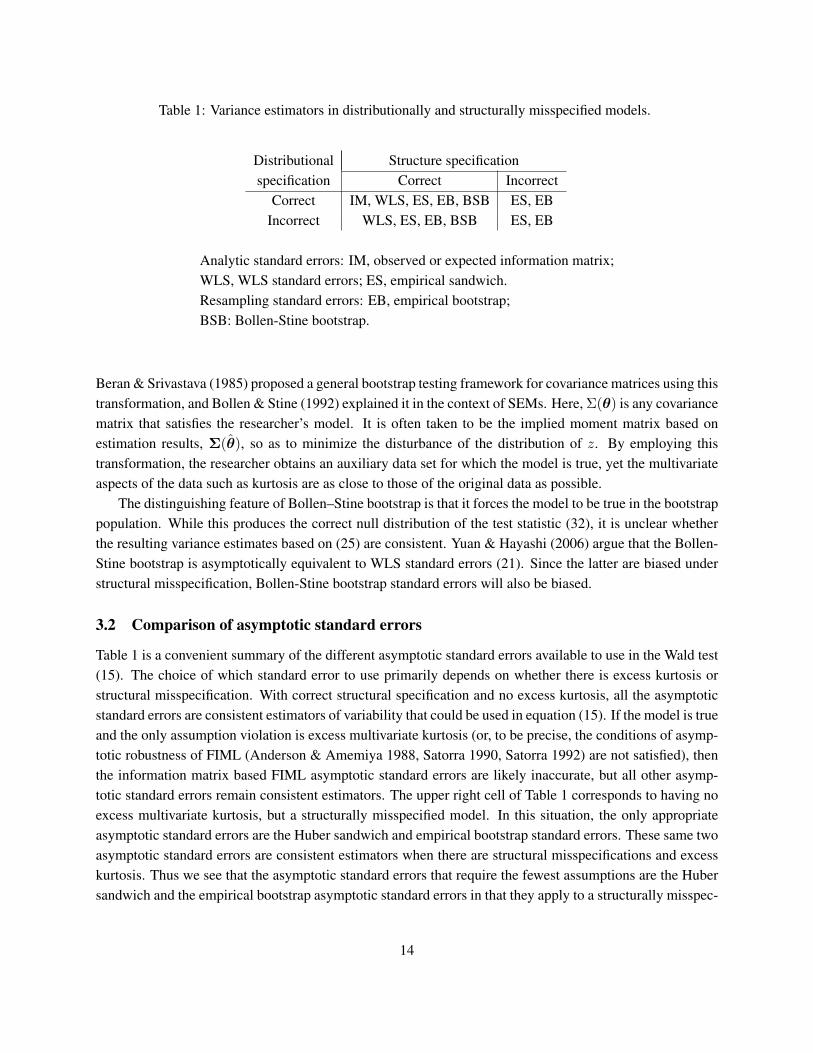
Table 1: Variance estimators in distributionally and structurally misspecified models.

Distributional Structure specificationspecification Correct Incorrect

Correct IM, WLS, ES, EB, BSB ES, EBIncorrect WLS, ES, EB, BSB ES, EB

Analytic standard errors: IM, observed or expected information matrix;WLS, WLS standard errors; ES, empirical sandwich.Resampling standard errors: EB, empirical bootstrap;BSB: Bollen-Stine bootstrap.

Beran & Srivastava (1985) proposed a general bootstrap testing framework for covariance matrices using thistransformation, and Bollen & Stine (1992) explained it in the context of SEMs. Here, Σ(θ) is any covariancematrix that satisfies the researcher’s model. It is often taken to be the implied moment matrix based onestimation results, Σ(θ), so as to minimize the disturbance of the distribution of z. By employing thistransformation, the researcher obtains an auxiliary data set for which the model is true, yet the multivariateaspects of the data such as kurtosis are as close to those of the original data as possible.

The distinguishing feature of Bollen–Stine bootstrap is that it forces the model to be true in the bootstrappopulation. While this produces the correct null distribution of the test statistic (32), it is unclear whetherthe resulting variance estimates based on (25) are consistent. Yuan & Hayashi (2006) argue that the Bollen-Stine bootstrap is asymptotically equivalent to WLS standard errors (21). Since the latter are biased understructural misspecification, Bollen-Stine bootstrap standard errors will also be biased.

3.2 Comparison of asymptotic standard errors

Table 1 is a convenient summary of the different asymptotic standard errors available to use in the Wald test(15). The choice of which standard error to use primarily depends on whether there is excess kurtosis orstructural misspecification. With correct structural specification and no excess kurtosis, all the asymptoticstandard errors are consistent estimators of variability that could be used in equation (15). If the model is trueand the only assumption violation is excess multivariate kurtosis (or, to be precise, the conditions of asymp-totic robustness of FIML (Anderson & Amemiya 1988, Satorra 1990, Satorra 1992) are not satisfied), thenthe information matrix based FIML asymptotic standard errors are likely inaccurate, but all other asymp-totic standard errors remain consistent estimators. The upper right cell of Table 1 corresponds to having noexcess multivariate kurtosis, but a structurally misspecified model. In this situation, the only appropriateasymptotic standard errors are the Huber sandwich and empirical bootstrap standard errors. These same twoasymptotic standard errors are consistent estimators when there are structural misspecifications and excesskurtosis. Thus we see that the asymptotic standard errors that require the fewest assumptions are the Hubersandwich and the empirical bootstrap asymptotic standard errors in that they apply to a structurally misspec-

14

ified model with observed variables from a distribution with excess multivariate kurtosis. It is yet unclearwhether the empirical bootstrap or the Huber sandwich standard errors would be preferable in a given finitesample situation. While the bootstrap is often viewed as a finite-sample method, its justifications are stillasymptotic. Our simulations (Section 4) provide some evidence on these issues.

3.3 Confidence intervals

A second way of checking H0 : θk ≥ 0 vs. H1 : θk < 0 and hence to check structural misspecification isto form a confidence interval (CI) around the variance estimate and to see whether the upper limit includesnonnegative values. There are two common ways to construct confidence intervals: by using asymptoticnormality and the asymptotic standard errors (analytical approach), or by using the bootstrap (resamplingapproach).

In general, the analytical two-sided confidence interval is

θ ± z1−α2× s.e.(θ) (27)

where θ is the parameter estimate, s.e.(θ) is the asymptotic standard error of θ, and z1−α2

is the correspond-ing percentile of the standard normal distribution determined by the Type I error probability. Analyticalconstruction of the confidence intervals leads to the inference outcomes identical to those of Wald tests fora single parameter. If the true value is outside the confidence interval, it also means that the z-score of theWald test exceeds the critical value, and so does the χ2

1 Wald test statistic. The confidence intervals andWald tests are parallel to one another.

Since we are interested in one-sided hypotheses tests (14), we would also be interested in one-sidedanalytical confidence intervals

(−∞, θ + z1−α × s.e.(θ)) (28)

analogous to the one-sided hypothesis testing problem. Again, rejection of the one-sided test is identical tolack of coverage of the true value by the one-sided CI.

As was true for the Wald test (15), there are several choices for the asymptotic standard errors. Whichone is appropriate depends on whether the distributional assumptions are satisfied for the observed variablesand whether the model is correctly specified. The discussion on asymptotic standard errors from the sectionon Wald tests carries over to the confidence intervals and we will not repeat it here except to say that ifthe assumptions that underlie the asymptotic standard errors do not hold, then the accuracy of the standarderrors and the confidence intervals that depend on them cannot be guaranteed.

An alternatve approach to construction of the confidence intervals is based on the bootstrap. Using thebootstrap framework of section 3.1.4, the two-sided bootstrap percentile confidence interval of level 1 − αis

(θ[Bα/2]∗ , θ

[B(1−α/2)]∗ ) (29)

where θ[1]∗ ≤ θ

[2]∗ ≤ . . . ≤ θ

[B]∗ are ordered bootstrap realizations of the estimate θ. A one-sided confidence

interval of level α is(−∞, θ[B(1−α)]

∗ ). (30)

15

Regardless of how a confidence interval was constructed, our CI-based test of the Heywood case consistsof verifying whether the confidence interval covers zero. If it does not, it should be viewed as evidenceagainst the null hypothesis of correct structural specification.

3.3.1 The Bollen-Stine bootstrap test

Another way to control for lack of multivariate normality and asymptotic robustness is to utilize the Bollen-Stine rotating bootstrap. To ensure that the distribution corresponds to the null hypothesis, the matrix Σ(θ)must come from a model in which the relevant Heywood case is eliminated by replacing θk = 0. Otherestimates necessary to construct Σ(θ) are obtained by maximization subject to this constraint. The p-valueof the Bollen-Stine bootstrap test is the proportion of times the actual estimate θk is below the estimated θ(b)

k∗in the b-th bootstrap sample:

p =1B

∑b

1I[θk < θ

(b)∗]

(31)

3.4 Likelihood ratio tests

Likelihood ratio (LR) tests or “chi-square” tests are another tool for testing statistical significance in SEMsestimated with FIML. The most widely used LR test in SEM is of H0 : Σ = Σ(θ) & µ = µ(θ). This is atest of whether the overidentification restrictions implied by the whole model hold. The moment structurehypothesis in (6) is tested by forming

T = NFFIML[θ] (32)

where N is the sample size,6 and then under the null hypothesis T asymptotically follows a χ2 distributionwith degrees of freedom equal to r = 1

2(p+ q)(p+ q + 3)− t where t is the number of distinct parametersin θ.

In addition, when one model is nested within another by imposing some equality restrictions (leadingto two-sided tests; see Sec. 3.4.3), the difference in the test statistics for the two nested models forms anasymptotic chi square statistic to test whether the most restricted of the two model fits as well as the lessrestrictive one. If the model is estimated with and without restrictions imposed by the null hypothesis,then the LRT statistic T is twice the difference of the log-likelihoods (7), or N times the difference of theminimized values of the objective function (8):

T = −2(l(θ0, Z)− l(θ1, Z)) = N[FFIML

(Σ(θ1), S

)− FFIML

(Σ(θ0), S

)],

θ0 = arg maxθ∈Θ0

l(θ, Z), θ1 = arg maxθ∈Θ1∪Θ0

l(θ, Z) (33)

3.4.1 Scaled and adjusted tests

When the observed variables come from a distribution with excess kurtosis and the asymptotic robustnessconditions are not met, the (quasi-)likelihood ratio test statistic (32) loses its pivotal χ2 form and becomes a

6 Sometimes, N − 1 is used as a multiplier, which is asymptotically equivalent to (32).

16

sum of weighted χ2:

Td−→

r∑j=1

αjXj , Xj ∼ i.i.d.χ21. (34)

Scalars αj are eigenvalues of the matrix U0Ω with

U0 = V − V∆0 (∆0′V∆0 )−1∆0

′V, (35)

where ∆0 and V were defined in section 3.1.2. Satorra & Bentler (1994) proposed to use the scaled statistic

Tsc =T

c, c =

1r

tr[U0ΩN ] (36)

referred to χ2r , and adjusted statistic

Tadj =d

cT, d =

(tr[U0Ω])2

tr[(U0ΩN )2](37)

referred to χ2d

where the degrees of freedom d might be a non-integer number. Here U0 is (35) evaluated at

θ. These are standard tests implemented in most SEM software packages.We can also implement the scaling version Satorra-Bentler corrections (36) to test nested models (Satorra

& Bentler 2001). If T1 and T2 are the χ2 goodness of fit statistics for two nested models, r1 and r2 arerespective degrees of freedom, and c1 and c2 are Satorra-Bentler scaling corrections, then Satorra-Bentlerscaled difference test can be computed as

Td =T1 − T2

cd,

cd =r1c1 − r2c2

r1 − r2(38)

referred to χ2 with r1 − r2 degrees of freedom. Again, this test is relevant for the two-sided situation (41).

3.4.2 Tests on the boundary of the parameter space

To apply the standard or corrected chi square tests to our hypotheses about negative variances introducescomplications. Recall that our null and alternative hypotheses are H0 : θk ≥ 0 vs. H1 : θk < 0, that is,a one-sided test. For one-sided testing (14), the asymptotic distribution of the usual likelihood ratio testdepends on the true value of the parameter. We distinguish two cases.

In the generic null situation when the true value of θk is strictly greater than zero, its (consistent)unrestricted estimate θk1 will also tend to be positive in large samples. By the law of large numbers,Prob[θk1 > 0] → 1 as N → ∞. If θk1 > 0, the estimates with and without the constraints imposedby the null hypothesis coincide, thus giving T b = 0. (Superscript b stands for the effect of the bound-ary of the parameter space.) Negative values, on the other hand, produce non-zero values of the statisticT b, but the probability of negative values decreases to 0 as the sample size increases to infinity (Savalei &Kolenikov 2008).

17

In the special case, still under the null hypothesis, that θk = 0 (i.e., we have found a perfect indicatorof a latent variable, which is questionable), θk1 will take positive and negative values approximately halfof the time each. While the positive values produce T b+ = 0, the negative values produce the test statisticT b− =

(θk1/s.e.[θk1]

)2. The latter has the distribution function Prob[T b− < t] = Prob[Z2 < t|Z < 0] =Prob[Z2 < t] = Prob[χ2

1 < t], where Z is a standard normal variate, and the conditioning in the secondequality is irrelevant since the distribution of Z2 is the same for both positive and negative values of Z.Overall, the asymptotic distribution is given by a mixture (Chernoff 1954, Perlman 1969, Shapiro 1985,Andrews 1999, Andrews 2001, Savalei & Kolenikov 2008),

Prob[T b ≤ c]→

0, c < 0,12 + 1

2 Prob(χ21 < c), c ≥ 0

(39)

We shall denote this asymptotic distribution by 12χ

20 + 1

2χ21; it is also known as χ distribution (Kudo 1963).

This is the most conservative distribution across all possible null hypotheses, most favorable for any al-ternative. Only with this distribution can a test with a non-trivial asymptotic size different from 0 or 1 bedeveloped.

Note that distribution (39) of the likelihood ratio test statsitic will only work with a single parameter.Furthermore, the asymptotic distribution for the test statistic, T b, is only applicable when the distributionalassumption for the observed variables is met (i.e., there is no excess kurtosis) and that the structural speci-fication is correct. To account for the effect of the boundary in the situations where asymptotic robustnessconditions are violated, we can consider an appropriate modification of the scaled difference test (38). If thevariance estimate in question is positive, the test statistic T bd is zero, while if the estimate is negative, it iscomputed according to (38). The overall distribution of the test is approximately

Prob[T bd ≤ c] ≈

0, c < 0,12 + 1

2 Prob(χ21 < c), c ≥ 0

(40)

The quality of the approximation depends on whether the two-sided scaled difference statistic (38) is wellapproximated by the χ2 distribution with one degree of freedom. If it is, then the approximation (40)improves with the sample size.

Note that tests on the boundary are still intended to test the null situation (14) of correct specification.The test (39) will work under no excess multivariate kurtosis, and test (40), under arbitrary kurtosis, but theyboth assume the model is correctly specified. If the model is structurally misspecified, the distributions ofthese tests will be different from the 1

2χ20 + 1

2χ21 mixture. Savalei & Kolenikov (2008) discuss in detail the

asymptotic and finite sample approximations that this test utilizes.

3.4.3 Two-sided tests

The last subsection explained the difficulty with testing the one sided hypothesis of H0 : θk ≥ 0 vs.H1 : θk < 0. Different null and alternative hypotheses tied to tests of negative variances are somewhatsimpler to handle:

H0 : θk = 0

H1 : θk 6= 0 (41)

18

Here the null hypothesis is that the variance is zero. This is the smallest plausible value consistent witha model being correctly specified. If θk were an indicator error variance, then H0 implies that there isno measurement error in the indicator; if θk were the error variance of an equation, then H0 implies thatthere is no error in predicting the outcome; and finally if θk were the variance of a latent variable, thenH0 implies that the latent variable does not exist. The alternative hypothesis is not directional, though inpractice the test would likely be applied when the sample variance estimate is negative and the researcherwants to determine whether it is within sampling error of zero. However, there are occasions where evena positive variance estimate might result in a test of H0 : θk = 0. For instance, a researcher might wantto test for the presence of a latent variable and the variance estimate of the variable is positive but small.TestingH0 : θk = 0 could provide evidence as to the existence of the latent variable. More generally, testingH0 : θk = 0 is a different setup that could provide evidence relevant to negative variances even though thealternative hypothesis is nondirectional. The two-sided LR test is more straightforward than the one-sidedtests described in the previous subsection. A nested chi square difference test is available where the model isfirst estimated without any constraints on the variances (unrestricted model) and then estimated when settingthe problematic variance to zero. An LR test that compares the restricted and unrestricted form is a test ofH0 : θk = 0. Rejection means a significance difference of the variance from zero. If the sample estimate isnegative it suggests a structurally misspecified model.

3.4.4 Signed root tests

As noted in the discussion of expression (14), our interest lies in one-sided tests of Heywood cases, whilethe tests just discussed are two-sided tests of H0 : θk = 0 vs. H1 : θk 6= 0. There is a class of tests thataddresses the desire for one-sided alternative hypotheses known as signed root tests. For those tests, thesquare root of the likelihood ratio is assigned the sign of the difference of the parameter estimate from itstarget:

r(θ0) = sign[θ − θ0]√T (42)

to yield an asymptotically standard normal distribution of r(·). The theory of the signed root tests is givenby Barndorff-Nielsen & Cox (1994), and examples of the practical use in social science applications weregiven by Andrews (2007).

By analogy, let us define the signed root of the scaled χ2 difference test:

rsc(θ0) = sign[θ − θ0]√Td. (43)

To the extent that the distribution of Td can be approximated by χ21, the distribution of rsc(·) can be approx-

imated by the standard normal distribution. Hence, the one-sided signed root tests of (14) reject H0 when,similarly to (16),

r(θ0) < zα orrsc(θ0) < zα (44)

Either the Bollen-Stine bootstrap or the Satorra-Bentler corrections enable researchers to test H0 : θk =0 vs. H1 : θk 6= 0 even when the usual distributional assumptions are violated. However, both of these likethe standard LR test assume that there is no structural misspecificaiton. This is a limitation of these testssince if θk < 0, then the model is structurally misspecified and the accuracy of any of the tests presented

19

in this subsection are open to question. To characterize the performance of this test, we need to be able todescribe its distribution under the null (i.e., when θk = 0) and under the alternative (i.e., when θk < 0).Either of them may be tricky if we admit a possibility that the model is misspecified.

Let us now relate the signed root tests (42) and (43) to the tests at the boundary (39) and (40). Foreither of them to reject the null, the parameter estimate θk1 must be negative, and the (straight or scaled)likelihood ratio difference must be greater than the critical value χ2

1,0.95 for a 5% level test, say. Hencethese tests are algebraically equivalent to one another, and application of either one will be dictated by theconvenience of the estimation results manipulation by the researcher. Currently, no SEM software providesany of these tests, but they can be easily incorporated in general statistical software packages, such as Stataor R, that allow arbitrary transformations of estimation results along with the functions to compute the tailprobabilities and quantiles of the basic statistical distributions.

Note also that since the Wald tests and likelihood ratio tests are asymptotically equivalent for the two-sided hypotheses (Buse 1982), their one-sided equivalence follows once the sign of the estimate is accountedfor. Thus not only the signed roots and the tests at the boundary are identical in finite samples, but they arealso close to the one-sided Wald test (16) in large samples.

3.5 Multiple and conditional tests of negative variances

In practice, a researcher will scan the output to detect inadmissible estimates and will only test those vari-ances that are negative. A reviewer noted that this conditional procedure with many parameters in questionmay produce inaccurate rejection probabilities and p-values. First, potentially there are as many tests ofHeywood cases, even though informal ones, as there are variance parameters in the model. Second, theformal tests, like the ones suggested above, are only performed when a negative estimate is observed, i.e.,after the researcher had “peeked” at the data. We shall analyze these two issues in turn.

In our experience, multiple negative variances are possible, but rare in practice. On the face of it, a singlenegative error variance leads to a single significance tests and the issue of multiple testing does not emerge.However from another perspective an informal test for negative variances happens as a researcher scans theresults of SEM to highlight only the negative values. One could argue that this scanning of values is aninformal significance test in that positive variance values are determined to not be statistically significantlynegative population variances. From this perspective, a researcher is performing as many significance testsas there are variances in the model and only performing formal tests when the variance estimate is negative.If we accept this argument, then we have a multiple testing problem where there are a large number ofsignificant tests performed albeit most are informal. This multiple testing leads the usual Type I errorprobabilities of finding a significant negative variance to be higher than estimated with the usual singletest probability. If, for instance, there are 20 variances in a model and the estimates for all but one arenonnegative and if we test the statistical significance for the negative one, the probability of finding itstatistically significant is higher than the nominal Type I error probability since we ”tested” (or checked)the other 19 variances to make sure they were positive. An implication of this is that we should set the TypeI error probability lower than the usual 0.05 level when testing the negative error variances to reflect thenumber of variances that are tested to be negative. A Bonferroni or Holm correction for multiple testingcould prove helpful especially when using the single parameter tests of statistical significance.

20

An advantage of the single tests of variances is that some of these are available for one-sided tests(H0 : θk ≥ 0 vs. H1 : θk < 0) and in the case of the Wald test, the Huber sandwich asymptotic standarderrors that underlie them apply even with structural misspecification. If a two-sided test of H0 : θk = 0vs. H1 : θk 6= 0 applies, then there is another option to test multiple hypotheses. Using the appropriatevariance-covariance matrix of the parameter estimator, a Wald test can be constructed as special cases of thegeneral linear hypothesisH0 : Cθ = c. If the estimates of θ are asymptotically normal, the Wald test statistic(Buse 1982, Amemiya 1985, Davidson & MacKinnon 1993, Ferguson 1996) is formed as a quadratic forminvolving the parameters and restrictions of interest:

W = (Cθ − c)T (CVCT )−1(Cθ − c) (45)

that has an asymptotic χ2 distribution with the degrees of freedom equal to the effective number of hypothe-ses tested (rank of C). Note that this result, unlike the likelihood ratio χ2, does not depend on normalityof underlying data, provided the estimator V[θ] is consistent. On the other hand, Wald tests are known tobe sensitive to alternative non-linear specifications (Lafontaine & White 1986, Phillips & Park 1988) andhence to re-parameterization (Gonzalez & Griffin 2001). The advantage of this simultaneous test is that itwill test whether all variances are significantly different from zero. A disadvantage of it is that given its nullhypothesis, it does not discriminate between variances that are positive and significantly different from zerofrom those that are negative and significant where the latter are of greater interest.

A second issue is the possible impact of the conditional nature of the test for positive vs. negativevariance in the case of a single variance being tested. Does this conditioning on the sign of the initialestimate affect the size of the test? Let us consider a one-sided test with the asymptotic standard normaldistribution of the test statistic T and a critical value c, such as Wald test (16), T = θ/s.e.[θ], or a signedroot test (44), T = sign[θ]

√Td. The probability that we reject H0 : θ ≥ 0 is the unconditional probability,

Prob[T < c]. If a researcher only testsH0 when the sample variance is negative, then the resulting rejectionprobability is Prob[T < c ∩ T < 0] = Prob[T < c|T < 0] Prob[T < 0]. The question becomes, whatis the relation between Prob[T < c] and Prob[T < c ∩ T < 0]? Let us rewrite the latter probability witha different conditioning as Prob[T < c ∩ T < 0] = Prob[T < 0|T < c] Prob[T < c]. We can see thatif the first conditional probability in the RHS is equal to 1, then the rejection probability upon conductingan informal screening is the same as the total rejection probability Prob[T < c]. Obviously, if the criticalvalue c < 0, then Prob[T < 0|T < c] = 1. The conditional probability of testing for negative errorvariances only if the variance is negative is equivalent to the unconditional probability of testing whether Tis less than the critical value. The latter can be set to the desired level by choosing c to be the correspondingpercentile of the standard normal distribution, and for test levels less than 50%, c will be negative for thetest of H0 : θ ≥ 0. No adjustment is needed.

In sum, we need to take account of the multiple tests implicitly performed when we screen the variancesto check whether they are negative or positive. But we do not need to adjust our individual test when weonly perform the test for negative error variances. Of course, we are assuming that the test statistics have theappropriate distribution for the data and model examined. In particular, the Wald tests must utilize consistentstandard errors.

21

3.6 Summary of the tests

Table 2 summarizes the tests we are studying, and lists our expectations regarding their performance. Wedescribe the anticipated performance of the tests under correct and incorrect structural specification. Theanticipations under correct structural specification are based on what is already known in the literature, or asprojected for the one-sided tests based on the known characteristics of the two-sided counterparts. We alsocontrol for the situations where the normal theory inference is applicable (“Normal” columns of the table),and when it is violated (“Non-normal” columns, i.e., excess kurtosis or lack of asymptotic robustness). Thelatter situation rules out the tests based on the normal theory, i.e., uncorrected likelihood ratio tests and Waldtests/CIs based on information matrix.

We indicate which of the tests we expect to perform well in large samples (−−−→ α and→ α symbolsin the table), which of the tests we expect to demonstrate their asymptotic properties with relatively smallersample sizes (→ α symbol), and which tests are expected to have wrong size (α— symbol). If a test haswrong size, it disqualifies it from consideration under the alternative (N/A symbol). If a test does achievethe target size, at least asymptotically, it is of interest to consider its power, so as to compare different typesof tests (“power?” symbol).

Study of the confidence intervals allows for simultaneous assessment of levels of tests and their powerswhen the structure of a model is misspecified. The level of the test can be assessed by computing the fractionof times the confidence interval covers the true (negative) value, while the power of the test can be assessedby computing the fraction of times the confidence interval does not cover the null value of zero.

All versions of Wald tests are expected to have comparable power, provided that the standard errors areconsistent under misspecification. We expect this consistency to hold for empirical sandwich and empiricalbootstrap standard errors, and we expect the information matrix based, WLS and Bollen-Stine bootstrapstandard errors to be biased down under misspecification. Two-sided tests are expected to have power lowerthan their one-sided counterparts. However no other comparisons of power can be made at this stage.

The large sample power of the local Wald test (16) can be found using asymptotic normality of theestimates. As √

N(θk − θ0k) ≈ N(0, Vk),

where Vk is the asymptotic variance found as the appropriate diagonal element of the asymptotic variance-covariance matrix (24), we can find

Prob[θk/s.e.[θk] < zα]

= Prob[(θk − θ0k)/

√Vk/N ·

√Vk/N/s.e.[θk] + θ0k/

√Vk/N ·

√Vk/N/s.e.[θk] < zα

]≈ Prob[Z < zα − θ0k/

√Vk/N

]≡ Φ

(zα − θ0k/

√Vk/N

)(46)

which increases to 1 as N →∞ since θ0k is negative.The one-sided LR-type tests, the test correcting for the boundary and the signed root test, are asymptot-

ically equivalent to the Wald test. The same power calculation can be used for large samples.

22

Table 2: Tests of Heywood cases.

Structural specification: Correct MisspecifiedDistributional specification: Normal Non-normal Normal Non-normal

Wald testsInfo matrix s.e. (17) −−−→ α α— N/A N/A

WLS s.e. (21) −−−→ α −−−→ α N/A N/AEmpirical sandwich s.e. (24) −−−→ α −−−→ α power? power?Empirical bootstrap s.e. (25) −−−→ α(B) −−−→ α(B) power? power?

Bollen–Stine bootstrap s.e. (26) −−−→ α(B) −−−→ α(B) N/A N/AConfidence intervals

Info matrix s.e. (17) −−−→ α α— α— α—WLS s.e. (21) −−−→ α −−−→ α α— α—

Empirical sandwich s.e. (24) −−−→ α −−−→ α −−−→ α −−−→ α

power? power?Empirical bootstrap s.e. (25) −−−→ α(B) −−−→ α(B) −−−→ α(B) −−−→ α(B)

power? power?Bollen–Stine bootstrap s.e. (26) −−−→ α(B) −−−→ α(B) α— α—

Empirical bootstrap percentile (30) → α(B) → α(B) → α(B) → α(B)power? power?

Bollen–Stine bootstrap percentile (31) → α(B) → α(B) α— α—Likelihood ratio type tests

One-sided testsTest at the boundary (39) −−−→ α α— power? N/A

Scaled test at the boundary (40) −−−→ α −−−→ α power? power?Signed root of χ2-difference (42) −−−→ α α— power? N/A

Signed root of scaled difference (43) −−−→ α −−−→ α power? power?Two-sided tests

χ2-difference (41) −−−→ α α— power? N/AScaled difference (38) −−−→ α −−−→ α power? power?

Legend:→ α: the test achieves the target level with moderate sample sizes−−−→ α: the test needs large sample sizes to achieve the target levelα—: the test violates assumptions needed for correct Type I level(B): performance of the bootstrap scheme depends on the number of the bootstrap samples BN/A: power of the test cannot be assessed as its size cannot be controlled for

23

4 Simulation study

Negative error variance in the population means that a model is structurally misspecified. However, negativeerror variance also can occur due to sampling fluctuations when the true variance is close to zero, and samplesize is not very large. As Table 2 shows, there are numerous possible tests of negative error variances.Which of these tests work best in detecting that an error variance is significantly different from zero? Togauge the performance of different tests, we conducted simulations with the populations having Heywoodcases in the misspecified model. For this to happen, we fit structurally misspecified models to realisticcovariance matrices. In practical situations, researchers never know whether their models are true, and thusthe possibility of structural misspecification is non-negligible. Other studies of negative variances haverelied on simulations where the negative variances are due to sampling fluctuations. Our simulations areunique in that we design a study where a structural misspecification of a model creates a negative errorvariance in the population.

The simulation design includes two models: a saturated model with 3 observed variables, and an overi-dentified model with 4 observed variables, with modifications to allow for the null behavior with correctlyspecified models, and the alternative behavior with incorrectly specified models. We study several distribu-tions (normal, heavy-tailed t(5), and a non-elliptic distribution), a range of sample sizes (from 50 to 5000),and a variety of tests outlined in the previous section.

We are interested in several inference outcomes, both in terms of the behavior under the null (keeping thesize of the test and coverage of the confidence intervals under control), and under the alternative (relativepowers of the tests that have the correct size). A large number of replications per each combination ofsettings is required to estimate (small) probabilities of type I error. The use of the same data sets forestimation with different types of standard errors can be viewed as a variance reduction technique (Skrondal2000).

All variables were generated with means of zeroes, and the models were estimated in deviation scores,so that the means and intercepts could be ignored. The simulations were performed in Stata SE statisticalsoftware (Stata Corp. 2007) using the estimation package confa for confirmatory factor analysis modelestimation (Kolenikov 2009). Stata’s internal maximum likelihood estimation routine ml yields the pointestimates and the estimated covariance of the parameter estimates using one of the observed information,outer product of the gradients, and empirical sandwich estimator (referred in Stata as “robust” estima-tor; not to be confused with WLS standard errors (21), which are implemented in confa package withvce(satorrabentler) option). The necessary gradients are computed by Stata numerically, with a lotof attention given to computational accuracy (Gould, Pittblado & Sribney 2006).

A complete summary of the simulation results would involve 4 models × 3 distributions × 7 samplesizes ×

[8 parameters × (7 standard error estimates + 7 associated Wald tests + characterization of bias

+ 8 possible bootstrap tests) + 4 likelihood ratio and related tests]

= 15, 792 characteristics to look at.An even greater number would arise if different measures of performance (e.g., mean, median, variance,quintiles, etc.) are used for these characteristics. Hence we are forced to present only a brief overview ofthe simulation results.

24

4.1 Three variables, saturated model

This example is designed to illustrate how using a false model might generate a Heywood case that is notpresent in the true model. The true data generating process is that of simultaneous equations:

V[y1] = 1y2 = 0.3y1 + ζ2, V[ζ2] = 1,y3 = 0.55y1 + 0.8y2 + ζ3, V[ζ3] = 1,

Σ =

1 0.3 0.790.3 1.09 1.0370.79 1.037 2.264

(47)

Suppose a researcher incorrectly believes that a confirmatory factor analysis (CFA) model

yk = λkξ + δk, k = 1, 2, 3 (48)

should be fitted to the data. To identify the scale of the latent variable, λ1 is set to 1. The model is exactlyidentified, and using the population covariance matrix (47), the values of the parameters can be computedanalytically to yield the population values

λ2 = 1.313, λ3 = 3.457, φ11 = 0.229, θ1 = 0.771, θ2 = 0.696, θ3 = −0.467

The Heywood case is observed with the third variable that has measurement error “variance” of −0.467.FIML estimates will converge to those values in large samples7, and hence the probability of observing aHeywood case when CFA is fit to the data coming from (47) will approach 100% as N →∞.

The models are depicted on Fig. 1 using the path analysis conventions (Bollen 1989). The regressioncoefficients are shown on the arrows, and the variances of the exogenous variables, factors and errors areshown in angular brackets. Panel (a) shows the true model generating process. Panel (b) shows the popu-lation parameters of the structurally misspecified CFA model. Panel (c) shows the parameters of the modelfitted with the variance of the last variable set to 0.

7 As discussed in Yuan & Chan (2005), different estimation procedures might have different probability limits when the modelis misspecified.

〈1〉

y1

y2

y3

ζ2〈1〉

ζ3〈1〉

0.3

0.55

0.8

.

1

y1 y2 y3

ξ1

δ1 δ2 δ3

〈0.229〉

11.313

3.457

〈0.771〉 〈0.696〉 〈−0.467〉

.

1

y1 y2 y3

ξ1

δ1 δ2 δ3

〈0.275〉

11.313

2.866

〈0.724〉 〈0.615〉 〈0〉

.

1

(a) (b) (c)

Figure 1: Population covariance structure with three variables: (a) data generating process, (b) fitted CFAmodel; (c) fitted CFA model with restricted variance. Population unique variances are in 〈angular brackets〉.

25

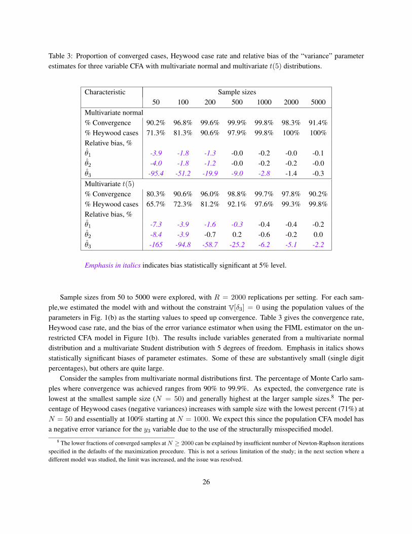
Table 3: Proportion of converged cases, Heywood case rate and relative bias of the “variance” parameterestimates for three variable CFA with multivariate normal and multivariate t(5) distributions.

Characteristic Sample sizes50 100 200 500 1000 2000 5000

Multivariate normal% Convergence 90.2% 96.8% 99.6% 99.9% 99.8% 98.3% 91.4%% Heywood cases 71.3% 81.3% 90.6% 97.9% 99.8% 100% 100%Relative bias, %θ1 -3.9 -1.8 -1.3 -0.0 -0.2 -0.0 -0.1θ2 -4.0 -1.8 -1.2 -0.0 -0.2 -0.2 -0.0θ3 -95.4 -51.2 -19.9 -9.0 -2.8 -1.4 -0.3Multivariate t(5)% Convergence 80.3% 90.6% 96.0% 98.8% 99.7% 97.8% 90.2%% Heywood cases 65.7% 72.3% 81.2% 92.1% 97.6% 99.3% 99.8%Relative bias, %θ1 -7.3 -3.9 -1.6 -0.3 -0.4 -0.4 -0.2θ2 -8.4 -3.9 -0.7 0.2 -0.6 -0.2 0.0θ3 -165 -94.8 -58.7 -25.2 -6.2 -5.1 -2.2

Emphasis in italics indicates bias statistically significant at 5% level.

Sample sizes from 50 to 5000 were explored, with R = 2000 replications per setting. For each sam-ple,we estimated the model with and without the constraint V[δ3] = 0 using the population values of theparameters in Fig. 1(b) as the starting values to speed up convergence. Table 3 gives the convergence rate,Heywood case rate, and the bias of the error variance estimator when using the FIML estimator on the un-restricted CFA model in Figure 1(b). The results include variables generated from a multivariate normaldistribution and a multivariate Student distribution with 5 degrees of freedom. Emphasis in italics showsstatistically significant biases of parameter estimates. Some of these are substantively small (single digitpercentages), but others are quite large.

Consider the samples from multivariate normal distributions first. The percentage of Monte Carlo sam-ples where convergence was achieved ranges from 90% to 99.9%. As expected, the convergence rate islowest at the smallest sample size (N = 50) and generally highest at the larger sample sizes.8 The per-centage of Heywood cases (negative variances) increases with sample size with the lowest percent (71%) atN = 50 and essentially at 100% starting at N = 1000. We expect this since the population CFA model hasa negative error variance for the y3 variable due to the use of the structurally misspecified model.

8 The lower fractions of converged samples atN ≥ 2000 can be explained by insufficient number of Newton-Raphson iterationsspecified in the defaults of the maximization procedure. This is not a serious limitation of the study; in the next section where adifferent model was studied, the limit was increased, and the issue was resolved.

26

We calculate the relative bias in Table 3 as

Rel. bias[θk] =1R

∑Ri=1 θ

(r)k − θk

θk× 100% (49)

where θ(r)k is the estimate of θk obtained in r-th simulated data set, and R is the number of Monte Carlo

replications. The (downward) biases are less than 5% for the error variances of y1 and y2 which are positivein the population model in Figure 1 b. However, the percentage bias for the error variance in y3 is very largeat the smaller sample sizes (-95.4% to -19.9% for N = 50 to N = 200). The significance of bias was testedby using a z-test of

H0 : E[θk,N ] = θk (50)

where the dependence of the distribution of θk on the sample size N is made explicit with a subindex. Thisis a z-test where the Monte Carlo results are used as the data, and the RHS value for the parameter of interestis taken from Fig. 1(b).

Variables from distributions with excess multivariate kurtosis can lead to inaccurate normal-theory basedstandard errors (Browne 1984, Satorra 1992). To explore this issue we used the same model, but generatedvariables from a multivariate t(5) distribution so as to create excess kurtosis leading to non-robust inference.The other parameters in the model were kept the same. The multivariate t distribution was obtained bysampling from the multivariate normal distribution first and dividing the resulting random data by

√V5/3,

V5 ∼ χ25 independent of the data. Note that this “difficult” distribution is unfavorable for WLS standard

errors. An estimate of the fourth order moments of the data is needed in (21), but it is not guaranteed tobe consistent for this distribution. Similar patterns of results are found with these non-normal data, butthe numeric values tend to indicate more severe problems. For instance, the proportion of converged casesis lower in the smaller sample sizes, and clear evidence of Heywood cases takes larger sample sizes toshow. In addition, the relative bias percent is larger and for some parameters does not disappear even atN = 5000, although it keeps decreasing in the absolute value. The explanation is in the excess kurtosis ofthis distribution which negatively affects both the bias and the variance of the estimates in finite samples,even though the estimates are consistent in accordance with Browne (1984).

Verification of the conjectures made in Table 1 is performed in Table 4 for analytic standard errors andselected variance parameters. The upper half of Table 4 corresponds to the upper right corner of Table 1,and describes performance of various types of standard errors in misspecified models with normal data.Reported measures include the Monte Carlo means and medians of the standard errors, as well as the MSEof the standard errors as a stability measure (Kovar, Rao & Wu 1988):

stability[vt(θ)

]=

∑Rr=1(v1/2

t,r [θ]− V[θ]1/2)2

V[θ]. (51)

Here t indexes the different variance estimator types, vt,r is the estimated variance reported in r-th MonteCarlo replication, and V[θ] = 1/R

∑Rr=1(θ(r) − ¯

θ)2 is the Monte Carlo variance of the parameter estimateθ. All types of standard errors are consistent, while information matrix standard errors are more stable.This is not surprising, as the IM standard errors are the maximum likelihood estimators, and hence areasymptotically efficient.

27

The bottom half of Table 4 corresponds to the lower right corner of Table 1, and describes performanceof various types of standard errors in misspecified models with non-normal data. In this case, the informationmatrix based standard errors are biased down to the point of being useless. Besides, they become less stableas the sample size increases beyond N = 500 or 1000, as the bias component dominates in the overall MSEin (51). The WLS and empirical sandwich standard errors exhibit great instability and skewness with lowsample sizes, but approach the target standard deviation as the sample size increases.

Seemingly contrary to the prediction of Table 1, WLS standard errors performed reasonably well in bothnormal and non-normal situations. This happened because the model was saturated, and hence σ∗ in (20)was identically zero. In this situation, WLS estimator (21) is appropriate.

The information matrix also performed well in the misspecified case with multivariate normal data.To explain this, we need to consider equation (20). There, the (asymptotic) normal theory weight matrix(11) is given by VN = .5D−(Σ ⊗ Σ)D−T , cancels with the variance of the moments Ω = 2D′(Σ ⊗Σ)D, and after some trivial algebra, the asymptotic variance becomes the inverse of the information matrix,1/N(∆V∆′)−1.

Let us now turn to tests of Heywood cases described in Table 2. Only calculations of the analyticaltests and standard errors were conducted for this model. Computationally intensive bootstrap simulationsfor both the empirical and Bollen–Stine bootstraps are conducted for another example and reported in thenext section. Calculation of the Satorra-Bentler scaled differences and their boundary-aware versions failedfor numerical reasons. When a saturated model is estimated without restrictions on θ3, computation of thescaling correction in (36) involves taking differences of two identical matrices resulting in a computer zero,and computation of the scaled test statistic involves division 0/0. The results were numerically unstable.

The results for the remaining tests are reported in Tables 5–6. To study sizes of the tests, the data wassimulated from the population shown on Fig. 1(c) with somewhat sparser grid of the sample sizes. If thecoverage of a CI is indeed 95%, then with 2000 Monte Carlo replications, the number of intervals that fail tocover the true parameter value is a binomial random variable with n = 2000 and p = 0.05, and the MonteCarlo standard deviation of coverage is

√0.95 · 0.05/2000 = 0.49%. We consider performance within

2% of the target 5% to be adequate. Such a high value is necessary to correct for multiple testing: eachsimulation results table we present reports about 100 test results. Performance outside of the 2% accuracymargin is indicated with italics. These italicized results raise questions about accuracy of the test for thesample size, data distribution and model specification.

Expectations put forward in Table 2 are by and large confirmed. All the tests achieve their target sizesin large samples. Poor performance of Wald tests and confidence intervals in small samples is likely dueto biases of parameter estimates, as the sampling distributions of θ3 have wrong centering. All other testsdemonstrate accurate performance. In particular, all likelihood ratio type tests have the right size in samplesas small as N = 100, which exceeded our expectations regarding these tests. However, this performancecritically hinges on the assumption of multivariate normality (or, more generally speaking, asymptotic ro-bustness). Once it is violated, as is the case with t(5) data, the likelihood ratio type tests break down.Likewise, the Wald tests and confidence intervals based on the normal theory information matrix standarderrors are clearly inappropriate. Wald tests with either WLS or empirical sandwich standard errors achievetheir target sizes asymptotically, although the sample sizes required for that exceed N = 1000. Confidenceintervals testing method shows good performance with some parameters, but requires large sizes for oth-

28

Table 4: Standards errors in the three variable confirmatory factor analysis model of Figure 1(b) (incorrectlyspecified model).

Characteristic Sample sizes50 100 200 500 1000 2000 5000

Multivariate normal dataHeywood case: θ3 (population value θ3 = −0.4667)MC s.d. 0.9477 0.7773 0.5221 0.3004 0.2057 0.1381 0.0849IM s.e.: Mean 1.0698 0.7680 0.5014 0.2952 0.2018 0.1401 0.0878

Median 0.7532 0.5814 0.4287 0.2755 0.1950 0.1385 0.0873Stability 1.4002 0.6917 0.2946 0.0892 0.0388 0.0181 0.0071

WLS s.e.: Mean 1.1999 0.8081 0.5035 0.2951 0.2015 0.1398 0.0877Median 0.7578 0.5814 0.4259 0.2754 0.1942 0.1380 0.0872

Stability 2.1096 0.8502 0.3403 0.0922 0.0403 0.0185 0.0077ES s.e.: Mean 1.2075 0.8104 0.5040 0.2951 0.2016 0.1399 0.0877

Median 0.7581 0.5814 0.4259 0.2754 0.1942 0.1380 0.0872Stability 2.2317 0.8747 0.3477 0.0925 0.0404 0.0185 0.0082

Non-Heywood case: θ1 (population value θ1 = 0.7715)MC s.d. 0.1634 0.1190 0.0839 0.0530 0.0379 0.0269 0.0166IM s.e.: Mean 0.1648 0.1190 0.0846 0.0540 0.0381 0.0270 0.0170

Median 0.1624 0.1179 0.0841 0.0539 0.0381 0.0270 0.0170Stability 0.0474 0.0232 0.0118 0.0050 0.0024 0.0012 0.0014

WLS s.e.: Mean 0.1607 0.1171 0.0838 0.0539 0.0381 0.0269 0.0170Median 0.1554 0.1152 0.0831 0.0537 0.0380 0.0269 0.0170

Stability 0.0665 0.0349 0.0184 0.0079 0.0039 0.0019 0.0017ES s.e.: Mean 0.1607 0.1172 0.0838 0.0539 0.0381 0.0269 0.0170

Median 0.1554 0.1152 0.0831 0.0537 0.0380 0.0269 0.0170Stability 0.0667 0.0350 0.0185 0.0079 0.0039 0.0019 0.0017

Multivariate t(5) dataHeywood case: θ3 (population value θ3 = −0.4667)MC s.d. 1.1327 0.9801 0.8127 0.5399 0.3039 0.2393 0.1530IM s.e.: Mean 0.9769 0.7321 0.5403 0.3189 0.2068 0.1433 0.0886

Median 0.6278 0.5224 0.4199 0.2724 0.1926 0.1374 0.0870Stability 0.8692 0.4871 0.3587 0.2660 0.1479 0.1808 0.1865

ES s.e.: Mean 1.4558 1.0963 0.8249 0.4873 0.3086 0.2257 0.1443Median 0.7333 0.6527 0.5456 0.3821 0.2761 0.2026 0.1336

Stability 3.7408 2.1162 1.5692 0.7391 0.1847 0.2604 0.1149WLS s.e.: Mean 1.4417 1.0903 0.8200 0.4866 0.3085 0.2256 0.1443

Median 0.7333 0.6526 0.5455 0.3820 0.2761 0.2026 0.1336Stability 3.4798 2.0353 1.4697 0.7223 0.1842 0.2595 0.1147

Non-Heywood case: θ1 (population value θ1 = 0.7715)MC s.d. 0.2243 0.1788 0.1336 0.0939 0.0640 0.0466 0.0320IM s.e.: Mean 0.1556 0.1153 0.0841 0.0539 0.0381 0.0269 0.0170

Median 0.1479 0.1114 0.0822 0.0531 0.0379 0.0268 0.0170Stability 0.1366 0.1447 0.1471 0.1778 0.1684 0.1804 0.2132

ES s.e.: Mean 0.1959 0.1610 0.1249 0.0863 0.0626 0.0458 0.0304Median 0.1685 0.1406 0.1113 0.0780 0.0581 0.0425 0.0281

Stability 0.2986 0.2786 0.1673 0.1383 0.0971 0.0932 0.0849WLS s.e.: Mean 0.1957 0.1610 0.1248 0.0863 0.0626 0.0458 0.0304

Median 0.1685 0.1406 0.1113 0.0779 0.0581 0.0425 0.0281Stability 0.2956 0.2781 0.1668 0.1381 0.0971 0.0932 0.0848

29

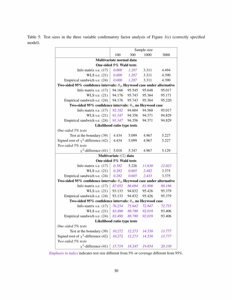
Table 5: Test sizes in the three variable confirmatory factor analysis of Figure 1(c) (correctly specifiedmodel).

Sample size100 300 1000 3000

Multivariate normal dataOne-sided 5% Wald tests

Info matrix s.e. (17) 0.000 1.287 3.311 4.494WLS s.e. (21) 0.000 1.287 3.311 4.390

Empirical sandwich s.e. (24) 0.000 1.287 3.311 4.390Two-sided 95% confidence intervals: θ3, Heywood case under alternative

Info matrix s.e. (17) 94.166 95.545 95.648 95.017WLS s.e. (21) 94.176 95.743 95.364 95.171

Empirical sandwich s.e. (24) 94.176 95.743 95.364 95.220Two-sided 95% confidence intervals: θ1, no Heywood case

Info matrix s.e. (17) 92.182 94.604 94.560 95.017WLS s.e. (21) 91.147 94.356 94.371 94.829

Empirical sandwich s.e. (24) 91.147 94.356 94.371 94.829Likelihood ratio type tests

One-sided 5% testsTest at the boundary (39) 4.434 5.099 4.967 5.227

Signed root of χ2-difference (42) 4.434 5.099 4.967 5.227Two-sided 5% tests

χ2-difference (41) 5.018 5.347 4.967 5.129Multivariate t(5) data

One-sided 5% Wald testsInfo matrix s.e. (17) 0.382 5.226 11.630 12.023

WLS s.e. (21) 0.282 0.605 2.482 3.375Empirical sandwich s.e. (24) 0.282 0.605 2.433 3.375

Two-sided 95% confidence intervals: θ3, Heywood case under alternativeInfo matrix s.e. (17) 87.052 86.094 81.800 80.186

WLS s.e. (21) 93.133 94.832 95.426 95.379Empirical sandwich s.e. (24) 93.133 94.832 95.426 95.379

Two-sided 95% confidence intervals: θ1, no Heywood caseInfo matrix s.e. (17) 76.254 75.642 72.847 72.755

WLS s.e. (21) 83.490 88.780 92.019 93.406Empirical sandwich s.e. (24) 83.490 88.780 92.019 93.406

Likelihood ratio type testsOne-sided 5% tests

Test at the boundary (39) 10.272 12.273 14.550 13.777Signed root of χ2-difference (42) 10.272 12.273 14.550 13.777Two-sided 5% tests

χ2-difference (41) 15.719 18.245 19.854 20.330

Emphasis in italics indicates test size different from 5% or coverage different from 95%.

30

ers. As a conservative suggestion, the asymptotic tests can be trusted with sample sizes N > 1000 in anon-normal situation for the current model size.

Table 6 compares the power of the tests. The combinations of sample sizes and distribution that wereidentified as problematic for the test size in Table 5 are repeatedly highlighted in Table 6. In the multi-variate normal situation, the best tests are the ones based on one-sided likelihood ratio tests (the boundarymodification and the signed root). They were shown to maintain accurate sizes for all sample sizes studied,and they also have the greatest power of all comparable tests. The power of the one-sided Wald tests isslightly smaller, and they need sample sizes aboveN = 1000 to have the right size. There are no discernibledifferences between Wald tests based on three different variance estimators (information matrix, WLS andempirical sandwich standard errors). Two-sided tests (based on likelihood ratio chi-square difference as wellas confidence intervals) have lower power, with likelihood ratio performing a little better. With multivariatet(5) data, only Wald tests and confidence intervals based on WLS or empirical sandwich standard errorsshowed appropriate test sizes in Table 5. Hence the normal theory inference results are excluded from con-sideration. The only meaningful power comparison is between the one-sided and two-sided tests. One-sidedtests have an advantage for the sample sizes N ≥ 2000 when such a comparison can be made.

Overall, when the model is saturated and the data are multivariate normal, one-sided modifications ofthe chi-square difference tests are the recommended tests. One-sided Wald tests or confidence intervals alsohave good power, but they only produce accurate test sizes in samples larger than N ≥ 500. When thenormality assumption is violated, the only means to construct Wald tests (or equivalent confidence intervals)are the WLS or empirical sandwich standard errors. One-sided intervals are preferred for one-sided testingsituations, but they require sample sizes N ≥ 2000 to ensure an accurate test size. Two-sided intervals havelower power, but they also work in smaller sample sizes (N ≥ 500).

As a conclusion for this model, it should be noted that proper testing of the Heywood case allows us toestablish that the model is inappropriate even when the overall fit test is not available due to the model beingexactly identified. We are not aware of any other approaches to test model fit in those situations.

31

Table 6: Power of the tests in the three variable confirmatory factor analysis of Figure 1(b), (incorrectlyspecified model).

Sample size50 100 200 500 1000 2000 5000

Multivariate normal dataOne-sided Wald tests

Info matrix s.e. (17) 0.000 0.309 7.781 53.677 85.159 99.238 100WLS s.e. (21) 0.107 0.406 8.763 53.777 85.293 99.290 100

Empirical sandwich s.e. (24) 0.107 0.355 8.763 53.777 85.293 99.290 100Two-sided confidence intervals: θ3, Heywood case, power

Info matrix s.e. (17) 1.598 0.566 1.155 31.066 72.809 97.815 100WLS s.e. (21) 1.974 0.660 2.203 31.916 72.186 97.719 100

Empirical sandwich s.e. (24) 1.974 0.660 2.203 31.866 72.186 97.719 100Two-sided confidence intervals: θ3, Heywood case, coverage

Info matrix s.e. (17) 89.477 91.662 94.026 95.348 94.970 95.681 94.809WLS s.e. (21) 88.794 91.066 94.542 95.148 94.547 95.590 95.455

Empirical sandwich s.e. (24) 88.794 91.066 94.542 95.198 94.547 95.590 95.455Confidence intervals: θ1, no Heywood case, coverage

Info matrix s.e. (17) 89.752 92.795 92.671 95.398 94.920 94.461 95.628WLS s.e. (21) 88.794 92.284 92.489 95.098 94.847 94.425 95.507

Empirical sandwich s.e. (24) 88.794 91.066 94.542 95.198 94.547 95.590 95.455Likelihood ratio type tests

One-sided testsTest at the boundary (39) 10.193 22.542 37.851 68.034 89.243 99.644 100

Signed root of χ2-difference (42) 10.193 22.542 37.851 68.034 89.243 99.644 100Two-sided tests

χ2-difference (41) 5.234 14.720 25.954 56.028 82.221 98.577 100Multivariate t(5) dataOne-sided Wald tests

WLS s.e. (21) 0.402 0.585 2.558 18.882 48.692 79.241 97.446Empirical sandwich s.e. (24) 0.402 0.585 2.558 18.882 48.692 79.241 97.446

Two-sided confidence intervals: θ3, Heywood case, powerWLS s.e. (21) 3.042 1.915 0.972 5.891 27.515 65.197 94.725

Empirical sandwich s.e. (24) 3.042 1.915 0.972 5.891 27.515 65.197 94.725Two-sided confidence intervals: θ3, Heywood case, coverageWLS s.e. (21) 84.615 88.085 90.435 93.303 94.970 94.772 94.392

Empirical sandwich s.e. (24) 84.615 88.085 90.435 93.303 94.970 94.772 94.392Confidence intervals: θ1, no Heywood case, coverage

WLS s.e. (21) 84.615 88.085 90.435 93.303 94.970 94.772 94.392Empirical sandwich s.e. (24) 84.615 88.085 90.435 93.303 94.970 94.772 94.392

Emphasis in italics indicates test size different from 5% or coverage different from 95%.

32

4.2 Four variables, overidentified model

To study the performance of the tests from Table 2 in an overidentified model, we used the populationrepresented in Fig. 2. Like in the population of Fig. 1, the true data generating model is that of recursiveregressions:

V[y1] = 1y2 = 0.9911y1 + ζ2, V[ζ2] = 1,y3 = 1.05y1 − 0.15y2 + ζ3, V[ζ3] = 0.8,y4 = 1.3y1 + 0.1y2 + ζ4, V[ζ4] = 0.7,

Σ =

1 0.9911 0.9013 1.3911

0.9911 1.9823 0.7433 1.48670.9013 0.7433 1.6349 1.29061.3991 1.4867 1.2461 2.6675

(52)

If the researcher studying the data fits an improperly specified confirmatory factor analysis model, thepopulation value of the variance of δ1 is exactly 0. This represents a quasi-null situation. The true model(panel (a)) is still that of recursive regressions (52), but the fitted CFA model does not produce an impropersolution: the population value of ψ1 is zero rather than negative. Hence this represents the null situation interms of the Heywood case setup (14), but an alternative situation in terms of the overall test (6) of correctlyvs. incorrectly specified structure of a model.

We generated the simulation data for this scenario using the multivariate normal and multivariate t(5)distributions. An additional non-elliptic distribution was also studied, in which ζ2 had log-normal distri-bution with parameters µ = 0.5043 and σ = 0.5. This log-normal distribution has variance equal to 1,moderate skewness equal to 1.750 and sizeable kurtosis equal to 8.898. Through the data generating regres-sion model, non-normality is propagated to the variables y2, y3 and y4.

Table 7 gives the descriptive statistics of the simulation. There were no convergence problems with anyof the distributions or sample sizes. The proportion of Heywood cases is about 50% across different samplesizes. All estimates show biases in small samples. Interestingly, when the data were generated accordingto the regression model with non-normal errors, the bias was not monotone, but rather was oscillating, withsample sizes N = 100 and N = 2000 exhibiting significantly positive bias, and other sample sizes belowN < 1000 exhibiting significantly negative bias.

y3

y1

〈1〉

y2

y4

ζ2

〈1〉

ζ3

〈0.8〉ζ4

〈0.7〉

0.9911

1.05

−0.15

1.3

0.1

.

1

y1 y2 y3 y4

ξ1

δ1 δ2 δ3 δ4

〈1〉

1

0.991 0.901

1.399

〈0〉 〈1〉 〈0.823〉 〈0.710〉

.

1

(a) (b)

Figure 2: Quasi-null covariance structure with four variables: (a) data generating process, (b) fitted CFAmodel.

33

Table 7: Proportion of converged cases, Heywood case rate and bias of the “variance” parameter estimatesfor incorrectly specified four variable confirmatory factor analysis model of Fig. 2(b).

Characteristic Sample sizes50 100 200 500 1000 2000 5000

Multivariate normal% Convergence 100% 100% 100% 100% 100% 100% 100%% Heywood cases 49.9% 51.1% 51.1% 49.8% 49.3% 49.7% 50.2%

Biasθ1 -0.0018 -0.0023 -0.0018 0.0001 0.0000 0.0001 -0.0001θ2 -0.0445 -0.0204 -0.0088 -0.0039 -0.0027 -0.0010 -0.0005θ3 -0.0270 -0.0150 -0.0079 -0.0036 -0.0012 -0.0016 0.0001θ4 -0.0290 -0.0153 -0.0052 -0.0039 -0.0002 -0.0007 0.0000Multivariate t(5)% Convergence 100% 100% 100% 99.97% 100% 100% 100%% Heywood cases 53.5% 50.5% 50.8% 50.3% 50.3% 50.3% 50.5%Biasθ1 -0.0128 -0.0044 -0.0018 -0.0006 -0.0003 -0.0004 -0.0001θ2 -0.0607 -0.0296 -0.0116 -0.0080 -0.0050 -0.0022 0.0001θ3 -0.0377 -0.0293 -0.0060 -0.0064 -0.0001 -0.0010 -0.0005θ4 -0.0301 -0.0263 -0.0155 -0.0064 -0.0025 -0.0004 -0.0001Lognormal ζ2 data% Convergence 99.96% 100% 100% 100% 100% 100% 100%% Heywood cases 54.8% 47.9% 51.9% 51.6% 48.8% 44.2% 50.4%Biasθ1 -0.0079 0.0022 -0.0017 -0.0014 -0.0019 0.0013 -0.0002θ2 -0.0298 -0.0240 -0.0114 -0.0019 -0.0030 -0.0021 -0.0011θ3 -0.0199 -0.0158 -0.0108 -0.0054 -0.0010 -0.0016 -0.0001θ4 -0.0154 -0.0172 -0.0044 -0.0023 -0.0019 -0.0034 -0.0007

Emphasis in italics indicates bias statistically significant at 1% level.

34

4.2.1 Standard errors

Table 8 reports the summary of the standard errors for the normal distribution. All types of standard errorsare biased down and asymmetric, especially with smaller samples. The bias is evident from comparisons ofthe mean reported standard error (the first line in each of the blocks) with the Monte Carlo standard deviationof the parameter estimates (top line of the table). Asymmetry of the distribution is evident from comparisonsof the means and medians of the standard error distributions. The empirical sandwich standard errors areabout 60% less stable than the information matrix based standard errors. Stability of the bootstrap standarderrors depends on the number of the bootstrap samples, with greater number producing more stable results.The empirical bootstrap standard errors tend to be less stable than the empirical sandwich standard errors.To obtain comparable stability, the number of the bootstrap replications must notably exceed the samplesize. While the Bollen-Stine bootstrap standard errors appear to perform well in smaller samples, they havea more pronounced downward bias in the larger samples. As a result their stability in the large samples isno better than that of the empirical bootstrap standard errors.

With non-normal elliptical Student t(5) data (Table 9), the variances of the estimates are larger thanin the normal case. However, the normal theory information matrix standard errors fail to account forthat, demonstrating 30–50% downward asymptotic bias, and even greater bias in small samples. The WLSstandard errors are asymptotically biased for the Heywood case, but not for the positive variance parameter.The factors behind this bias are explained in Section 3.1.2. The empirical bootstrap standard errors havelower bias and better stability than the empirical sandwich standard errors. The Bollen-Stine bootstrapstandard errors are comparable to the WLS standard errors, also suffering from asymptotic bias. Hence,based on this Table, the best performing method to compute standard errors when the data do not satisfy theasymptotic robustness conditions appears to be the empirical bootstrap.

Table 10 shows the standard errors obtained when the data were generated with non-normal errors. Thestandard errors for this distribution closely resemble those for the normal distribution. Hence it shouldbe concluded that the conditions of asymptotic robustness are satisfied for this distribution even thoughthe model is structurally misspecified. The patterns of performance of different types of standard errorsresembles the other two cases: the WLS and the Bollen-Stine bootstrap standard errors are biased down inlarger samples, while the empirical bootstrap standard errors can offer performance that beats other varianceestimation methods when the number of bootstrap samples is at least twice the sample size.

4.2.2 Test sizes

The next three tables describe the performance of the tests outlined in Table 2 in terms of their size. Usingthese tables, we want to identify the tests that have their target size of 5% under a wide variety of settings.Table 11 reports the results for the multivariate normal case. Except for a few tests that have problems atthe smallest sample size (N = 50, scaled and adjusted overall tests and their one-sided versions), most testsappear to perform well. Table 12 reports the summary of the test sizes for multivariate t(5) data. In thissituation, all of the normal theory based inferential procedures (Wald tests and confidence intervals basedon the information matrix standard errors; normal theory chi-square, chi-square difference and its one-sidedversions) break down completely. The small sample problems of the scaled and adjusted chi-square testsand the scaled difference tests affect samples of the size up to N ≤ 200. The bootstrap percentile tests

35

Table 8: Standards errors in four variable confirmatory factor analysis model of Figure 2(b), multivariatenormal data, incorrectly specified model with zero population variance of δ1.

Characteristic Sample sizes50 100 200 500 1000 2000 5000

Heywood case: θ1 (population value θ1 = 0)MC s.d. 0.0636 0.0432 0.0302 0.0190 0.0135 0.0094 0.0061IM s.e.: Mean 0.0598 0.0419 0.0297 0.0188 0.0133 0.0094 0.0060

Median 0.0576 0.0412 0.0295 0.0188 0.0133 0.0094 0.0060Stability 0.0387 0.0192 0.0098 0.0039 0.0020 0.0011 0.0005

WLS s.e.: Mean 0.0503 0.0365 0.0261 0.0166 0.0118 0.0084 0.0053Median 0.0484 0.0359 0.0259 0.0166 0.0118 0.0084 0.0053

Stability 0.0583 0.0293 0.0161 0.0063 0.0039 0.0026 0.0016ES s.e.: Mean 0.0608 0.0425 0.0300 0.0190 0.0134 0.0095 0.0060

Median 0.0577 0.0415 0.0296 0.0189 0.0134 0.0095 0.0060Stability 0.0598 0.0306 0.0170 0.0065 0.0035 0.0018 0.0008

EB s.e. (B = 60): Mean 0.0659 0.0300 0.0133Median 0.0608 0.0297 0.0133

Stability 0.0705 0.0246 0.0111EB s.e. (B = 300): Mean 0.0659 0.0302 0.0134

Median 0.0616 0.0295 0.0133Stability 0.0540 0.0191 0.0056

BSBPF s.e. (B = 60): Mean 0.0554 0.0275 0.0124Median 0.0531 0.0273 0.0125

Stability 0.0671 0.0257 0.0134BSBPF s.e. (B = 300): Mean 0.0576 0.0278 0.0124

Median 0.0539 0.0274 0.0124Stability 0.0636 0.0183 0.0061

BSBZV s.e. (B = 60): Mean 0.0543 0.0272 0.0124Median 0.0529 0.0270 0.0124

Stability 0.0656 0.0246 0.0132BSBZV s.e. (B = 300): Mean 0.0537 0.0274 0.0124

Median 0.0517 0.0272 0.0124Stability 0.0529 0.0163 0.0072

IM: information matrix; WLS: weighted least squares; ES: empirical sandwich; EB: empirical boot-strap; BSBPF: Bollen-Stine bootstrap with data rotated to Perfectly Fit the CFA model; BSBZV:Bollen-Stine bootstrap to fit the CFA model with Zero Variance.

36

Table 8: (continued).

Characteristic Sample sizes50 100 200 500 1000 2000 5000

Non-Heywood case: θ3 (population value θ3 = 0.823)MC s.d. 0.1671 0.1167 0.0847 0.0531 0.0370 0.0260 0.0165IM s.e.: Mean 0.1633 0.1164 0.0828 0.0527 0.0373 0.0264 0.0167

Median 0.1601 0.1158 0.0823 0.0526 0.0373 0.0264 0.0167Stability 0.1671 0.1167 0.0847 0.0531 0.0370 0.0260 0.0165

WLS s.e.: Mean 0.1551 0.1146 0.0832 0.0532 0.0378 0.0268 0.0170Median 0.1516 0.1130 0.0826 0.0531 0.0377 0.0268 0.0170

Stability 0.1671 0.1167 0.0847 0.0531 0.0370 0.0260 0.0165ES s.e.: Mean 0.1594 0.1150 0.0825 0.0525 0.0372 0.0264 0.0167

Median 0.1551 0.1128 0.0816 0.0523 0.0371 0.0263 0.0167Stability 0.1671 0.1167 0.0847 0.0531 0.0370 0.0260 0.0165

EB s.e. (B = 60): Mean 0.1618 0.0809 0.0372Median 0.1551 0.0797 0.0372

Stability 0.1723 0.0861 0.0369EB s.e. (B = 300): Mean 0.1591 0.0821 0.0371

Median 0.1561 0.0808 0.0371Stability 0.1723 0.0862 0.0369

BSBPF s.e. (B = 60): Mean 0.1518 0.0824 0.0375Median 0.1494 0.0819 0.0375

Stability 0.1723 0.0862 0.0369BSBPF s.e. (B = 300): Mean 0.1569 0.0831 0.0379

Median 0.1537 0.0825 0.0377Stability 0.1723 0.0862 0.0369

BSBZV s.e. (B = 60): Mean 0.1561 0.0834 0.0376Median 0.1529 0.0834 0.0374

Stability 0.1655 0.0843 0.0368BSBZV s.e. (B = 300): Mean 0.1567 0.0832 0.0381

Median 0.1541 0.0830 0.0378Stability 0.1655 0.0843 0.0368

IM: information matrix; WLS: weighted least squares; ES: empirical sandwich; EB: empirical boot-strap; BSBPF: Bollen-Stine bootstrap with data rotated to Perfectly Fit the CFA model; BSBZV:Bollen-Stine bootstrap to fit the CFA model with Zero Variance.

37

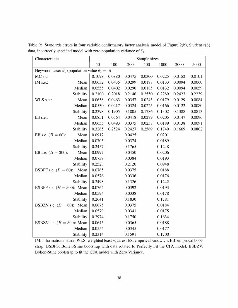
Table 9: Standards errors in four variable confirmatory factor analysis model of Figure 2(b), Student t(5)data, incorrectly specified model with zero population variance of δ1.

Characteristic Sample sizes50 100 200 500 1000 2000 5000

Heywood case: θ1 (population value θ1 = 0)MC s.d. 0.1098 0.0880 0.0475 0.0300 0.0225 0.0152 0.0101IM s.e.: Mean 0.0632 0.0435 0.0299 0.0188 0.0133 0.0094 0.0060

Median 0.0555 0.0402 0.0290 0.0185 0.0132 0.0094 0.0059Stability 0.2100 0.2018 0.2146 0.2550 0.2289 0.2423 0.2239

WLS s.e.: Mean 0.0658 0.0463 0.0357 0.0243 0.0179 0.0129 0.0084Median 0.0530 0.0417 0.0324 0.0225 0.0166 0.0122 0.0080

Stability 0.2398 0.1905 0.1805 0.1786 0.1302 0.1388 0.0813ES s.e.: Mean 0.0851 0.0564 0.0418 0.0279 0.0205 0.0147 0.0096

Median 0.0655 0.0493 0.0375 0.0258 0.0189 0.0138 0.0091Stability 0.3265 0.2524 0.2427 0.2569 0.1740 0.1669 0.0802

EB s.e. (B = 60): Mean 0.0917 0.0425 0.0201Median 0.0705 0.0374 0.0189

Stability 0.2457 0.1765 0.1248EB s.e. (B = 300): Mean 0.0997 0.0450 0.0206

Median 0.0738 0.0384 0.0193Stability 0.2523 0.2120 0.0948

BSBPF s.e. (B = 60): Mean 0.0765 0.0375 0.0188Median 0.0576 0.0336 0.0176

Stability 0.2498 0.1326 0.1242BSBPF s.e. (B = 300): Mean 0.0764 0.0392 0.0193

Median 0.0594 0.0338 0.0178Stability 0.2641 0.1830 0.1781

BSBZV s.e. (B = 60): Mean 0.0675 0.0375 0.0184Median 0.0579 0.0341 0.0175

Stability 0.2974 0.1750 0.1634BSBZV s.e. (B = 300): Mean 0.0645 0.0365 0.0188

Median 0.0554 0.0345 0.0177Stability 0.2314 0.1591 0.1700

IM: information matrix; WLS: weighted least squares; ES: empirical sandwich; EB: empirical boot-strap; BSBPF: Bollen-Stine bootstrap with data rotated to Perfectly Fit the CFA model; BSBZV:Bollen-Stine bootstrap to fit the CFA model with Zero Variance.

38

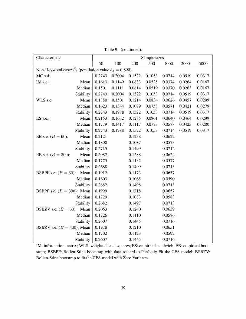
Table 9: (continued).

Characteristic Sample sizes50 100 200 500 1000 2000 5000

Non-Heywood case: θ3 (population value θ3 = 0.823)MC s.d. 0.2743 0.2004 0.1522 0.1053 0.0714 0.0519 0.0317IM s.e.: Mean 0.1613 0.1149 0.0833 0.0525 0.0374 0.0264 0.0167

Median 0.1501 0.1111 0.0814 0.0519 0.0370 0.0263 0.0167Stability 0.2743 0.2004 0.1522 0.1053 0.0714 0.0519 0.0317

WLS s.e.: Mean 0.1880 0.1501 0.1214 0.0834 0.0626 0.0457 0.0299Median 0.1623 0.1344 0.1079 0.0758 0.0571 0.0421 0.0279

Stability 0.2743 0.1988 0.1522 0.1053 0.0714 0.0519 0.0317ES s.e.: Mean 0.2153 0.1632 0.1285 0.0861 0.0640 0.0464 0.0299

Median 0.1779 0.1417 0.1117 0.0773 0.0578 0.0423 0.0280Stability 0.2743 0.1988 0.1522 0.1053 0.0714 0.0519 0.0317

EB s.e. (B = 60): Mean 0.2121 0.1238 0.0622Median 0.1800 0.1087 0.0573

Stability 0.2715 0.1499 0.0712EB s.e. (B = 300): Mean 0.2082 0.1288 0.0624

Median 0.1775 0.1132 0.0577Stability 0.2688 0.1499 0.0713

BSBPF s.e. (B = 60): Mean 0.1912 0.1173 0.0637Median 0.1603 0.1065 0.0590

Stability 0.2682 0.1498 0.0713BSBPF s.e. (B = 300): Mean 0.1999 0.1218 0.0657

Median 0.1729 0.1083 0.0583Stability 0.2682 0.1497 0.0713

BSBZV s.e. (B = 60): Mean 0.2053 0.1240 0.0639Median 0.1726 0.1110 0.0586

Stability 0.2607 0.1445 0.0716BSBZV s.e. (B = 300): Mean 0.1978 0.1210 0.0651

Median 0.1702 0.1123 0.0592Stability 0.2607 0.1445 0.0716

IM: information matrix; WLS: weighted least squares; ES: empirical sandwich; EB: empirical boot-strap; BSBPF: Bollen-Stine bootstrap with data rotated to Perfectly Fit the CFA model; BSBZV:Bollen-Stine bootstrap to fit the CFA model with Zero Variance.

39

Table 10: Standards errors in four variable confirmatory factor analysis model of Figure 2(b), lognormal ζ2,incorrectly specified model with zero population variance of δ1.

Characteristic Sample sizes50 100 200 500 1000 2000 5000

Heywood case: θ1 (population value θ1 = 0)MC s.d. 0.0634 0.0430 0.0298 0.0190 0.0131 0.0098 0.0060IM s.e.: Mean 0.0615 0.0417 0.0297 0.0186 0.0133 0.0094 0.0059

Median 0.0589 0.0410 0.0293 0.0185 0.0132 0.0094 0.0059Stability 0.0404 0.0217 0.0101 0.0037 0.0063 0.0013 0.0004

WLS s.e.: Mean 0.0507 0.0361 0.0263 0.0166 0.0118 0.0084 0.0053Median 0.0482 0.0353 0.0259 0.0165 0.0117 0.0084 0.0053

Stability 0.0603 0.0324 0.0161 0.0065 0.0059 0.0032 0.0010ES s.e.: Mean 0.0640 0.0422 0.0301 0.0187 0.0134 0.0095 0.0060

Median 0.0597 0.0411 0.0295 0.0186 0.0133 0.0095 0.0060Stability 0.0707 0.0343 0.0168 0.0067 0.0077 0.0021 0.0007

EB s.e. (B = 60): Mean 0.0720 0.0303 0.0133Median 0.0640 0.0296 0.0134

Stability 0.0633 0.0258 0.0156EB s.e. (B = 300): Mean 0.0708 0.0306 0.0134

Median 0.0623 0.0301 0.0134Stability 0.0673 0.0184 0.0086

BSBPF s.e. (B = 60): Mean 0.0583 0.0274 0.0123Median 0.0525 0.0270 0.0123

Stability 0.0706 0.0250 0.0119BSBPF s.e. (B = 300): Mean 0.0561 0.0277 0.0123

Median 0.0515 0.0274 0.0123Stability 0.0573 0.0181 0.0066

BSBZV s.e. (B = 60): Mean 0.0529 0.0275 0.0122Median 0.0505 0.0269 0.0121

Stability 0.0690 0.0220 0.0130BSBZV s.e. (B = 300): Mean 0.0544 0.0272 0.0123

Median 0.0520 0.0267 0.0123Stability 0.0590 0.0172 0.0056

IM: information matrix; WLS: weighted least squares; ES: empirical sandwich; EB: empirical boot-strap; BSBPF: Bollen-Stine bootstrap with data rotated to Perfectly Fit the CFA model; BSBZV:Bollen-Stine bootstrap to fit the CFA model with Zero Variance.

40

Table 10: (continued).

Characteristic Sample sizes50 100 200 500 1000 2000 5000

Non-Heywood case: θ3 (population value θ3 = 0.823)MC s.d. 0.1664 0.1231 0.0845 0.0528 0.0400 0.0259 0.0167IM s.e.: Mean 0.1635 0.1166 0.0824 0.0525 0.0373 0.0264 0.0167

Median 0.1608 0.1157 0.0822 0.0524 0.0373 0.0264 0.0167Stability 0.1664 0.1231 0.0845 0.0528 0.0400 0.0259 0.0167

WLS s.e.: Mean 0.1559 0.1151 0.0829 0.0533 0.0378 0.0269 0.0170Median 0.1522 0.1134 0.0823 0.0531 0.0377 0.0268 0.0170

Stability 0.1664 0.1231 0.0846 0.0528 0.0400 0.0259 0.0167ES s.e.: Mean 0.1604 0.1150 0.0819 0.0524 0.0372 0.0264 0.0167

Median 0.1552 0.1130 0.0812 0.0522 0.0372 0.0264 0.0167Stability 0.1664 0.1231 0.0845 0.0528 0.0400 0.0259 0.0167

EB s.e. (B = 60): Mean 0.1610 0.0813 0.0373Median 0.1531 0.0799 0.0371

Stability 0.1664 0.0852 0.0398EB s.e. (B = 300): Mean 0.1613 0.0815 0.0371

Median 0.1554 0.0806 0.0371Stability 0.1663 0.0852 0.0398

BSBPF s.e. (B = 60): Mean 0.1587 0.0825 0.0378Median 0.1550 0.0815 0.0377

Stability 0.1659 0.0852 0.0396BSBPF s.e. (B = 300): Mean 0.1540 0.0818 0.0378

Median 0.1512 0.0808 0.0377Stability 0.1656 0.0852 0.0396

BSBZV s.e. (B = 60): Mean 0.1537 0.0823 0.0378Median 0.1491 0.0814 0.0377

Stability 0.1606 0.0838 0.0392BSBZV s.e. (B = 300): Mean 0.1560 0.0821 0.0380

Median 0.1511 0.0809 0.0380Stability 0.1606 0.0838 0.0392

IM: information matrix; WLS: weighted least squares; ES: empirical sandwich; EB: empirical boot-strap; BSBPF: Bollen-Stine bootstrap with data rotated to Perfectly Fit the CFA model; BSBZV:Bollen-Stine bootstrap to fit the CFA model with Zero Variance.

41

appear to reject too often, although this finding is not very firm.Table 13 describes an interesting situation in which the structural model is misspecified, and the Hey-

wood case is exactly θ1 = 0 in the population. Since the model is structurally misspecified, WLS standarderror perform poorly, with confidence intervals being too narrow, and rejection rates being too high. Bollen-Stine bootstrap percentile test rejects too often with the smallest sample size. All other tests have the requiredsizes. Since the normal theory inference is not affected by the non-normality of the distribution, it should beconcluded that the assumptions of asymptotic robustness are satisfied for this model, contrary to what wasexpected given its structure.

4.2.3 Power of the tests

As indicated in the last two columns of Table 2, power comparisons are of interest for the tests with known(and identical) sizes.

Changing the values of the parameters in the model of Fig. 2 can create a population Heywood case. Forinstance, when the coefficient β12 of regression of y2 on y1 goes down to 0.6, a mild Heywood case appearswith θ1 = −0.006. The asymptotic power of Wald tests can be computed using (46) where the asymptoticvariance As.Var[ψ1] = 0.509/N for data from multivariate normal or asymptotically robust distributions.For the multivariate t(5) data, this variance needs to be increased by a factor of 5/3 to account for heaviertails of the distribution. The theoretical calculations are compared with the simulated power on Fig. 3.In simulations, 2000 Monte Carlo replicates were taken for the analytic results, and 1000 replicates for thebootstrap results. The theoretical power is given by the smooth curve. Different versions of the Wald test aregiven by circles for analytic standard errors, and by plus signs for Bollen-Stine bootstrap standard errors; thetwo-sided difference tests, by triangles; the one-sided difference tests, by X’s; and the percentile bootstraptests, by diamonds. The upper panel gives the results for the multivariate normal distribution; the middlepanel, for the multivariate t(5) distribution; and the lower panel, for the data with lognormal ζ2. Wald testsbased on the WLS standard errors were excluded from consideration, as they were biased when the modelwas misspecified. Also, the performance of the tests with the smallest sample sizes may be problematic, asshown in Tables 11–13. No clear ordering of the tests in terms of their power can be deduced from theseresults, except that the two-sided tests have lower power, as expected. The bootstrap percentile tests, as wellas one-sided difference (signed root) tests might have a slight advantage in small samples, but they wereshown in the aforementioned tables to have slightly elevated sizes. The distributionally robust scaled chi-square difference test had somewhat lower power for the non-normal data in Fig. 3(c) than other one-sidedtests. The power of all tests is lower in the multivariate t(5) case due to larger sampling variances of theestimates.

The low power of the tests in this example is caused by the population value of the Heywood casethat is very close to zero. We tried different sets of parameter values with the data generating model ofFig. 2, and other patterns of the power curves were produced. For instance, with β12 = 0.4, β13 = 0.8,β14 = 0.6, β23 = −0.1, β24 = −0.1, V[δ3] = V[δ4] = 1, the obtained Heywood case has a magnitudeof θ01 = −0.1951. Due to the larger magnitude of the Heywood case (or, to be precise, the ratio of theHeywood case value in population to the asymptotic variance of the corresponding estimate), the tests havenon-trivial power that approaches 1 in large samples. While the Wald tests perform poorly with sample sizes

42

Table 11: Test sizes in four variable confirmatory factor analysis model of Figure 2(b), multivariate normaldistribution, incorrectly specified model with zero population variance of δ1.

Misspecification Sample sizestest 50 100 200 500 1000 2000 5000

Wald testsIM s.e. 5.036 5.106 3.760 4.677 5.072 5.587 5.268

WLS s.e. 6.512 5.568 4.113 4.738 4.994 5.556 5.171ES s.e. 5.433 5.229 4.034 4.677 4.908 5.493 5.204

EB s.e. (B = 60) 4.686 4.518 5.025EB s.e. (B = 300) 4.289 3.755 5.448

BSBPF s.e. (B = 60) 5.707 4.521 5.532BSBPF s.e. (B = 300) 5.128 4.064 5.034

Confidence intervals (coverage)IM s.e. 94.964 95.171 94.869 95.723 94.928 94.941 94.215

WLS s.e. 92.609 93.725 94.595 95.508 94.597 95.034 94.215ES s.e. 94.087 94.432 94.634 95.508 94.519 95.003 94.247

EB s.e. (B = 60) 94.678 94.793 93.886EB s.e. (B = 300) 95.314 94.789 94.216

BSBPF s.e. (B = 60) 93.962 94.559 94.049BSBPF s.e. (B = 300) 94.210 95.322 94.379

Bootstrap percentile testsEB %-tile (B = 60) 7.943 5.666 5.779

EB %-tile (B = 300) 8.261 5.211 5.532BSBPF %-tile (B = 60) 7.361 5.977 6.203

BSBPF %-tile (B = 300) 7.858 4.985 5.453One-sided local tests

NT test at the boundary 6.782 5.350 3.911 4.750 5.285 5.727 5.181Scaled test at the boundary 8.354 6.250 4.218 4.750 5.369 5.626 5.181

Signed root of NT difference 6.782 5.350 3.911 4.750 5.285 5.727 5.181Signed root of scaled difference 8.354 6.250 4.218 4.750 5.369 5.626 5.181

Two-sided local testsχ2-difference 6.369 6.000 5.215 4.350 5.369 5.170 5.397

Scaled difference 8.271 7.050 5.215 4.700 5.369 5.220 5.505IM: information matrix; WLS: weighted least squares; ES: empirical sandwich; EB: empirical bootstrap;BSBPF: Bollen-Stine bootstrap with data rotated to fit the CFA model.Simulation margin of error: for analytic standard errors and tests,

√0.95 · 0.05/2000 = 0.49%; for the

bootstrap standard errors and tests,√

0.95 · 0.05/1000 = 0.69%. Emphasis in italics indicates test sizesdifferent from 5% or coverage different from 95% by 2% or more for analytic standard errors and tests, andby 3% or more for the bootstrap standard errors and tests.

43

Table 12: Test sizes in four variable confirmatory factor analysis model of Figure 2(b), multivariate t(5)distribution, incorrectly specified model with zero population variance of δ1.

Misspecification Sample sizestest 50 100 200 500 1000 2000 5000

Wald testsIM s.e. 9.164 11.333 12.831 13.486 14.180 14.939 15.512

WLS s.e. 7.813 7.145 6.479 6.124 5.302 5.543 5.386ES s.e. 5.084 5.621 5.255 5.784 5.064 5.262 5.448

EB s.e. (B = 60) 2.798 4.896 5.766EB s.e. (B = 300) 2.238 4.647 5.463

BSBPF s.e. (B = 60) 5.276 5.812 6.110BSBPF s.e. (B = 300) 4.480 4.962 5.349

Confidence intervals (coverage)IM s.e. 88.195 84.667 83.177 79.957 80.327 79.017 77.624

WLS s.e. 90.905 93.045 94.295 94.618 94.854 95.584 95.137ES s.e. 94.596 94.443 95.193 94.958 95.053 95.647 95.199

EB s.e. (B = 60) 95.923 94.357 95.068EB s.e. (B = 300) 96.563 95.104 94.537

BSBPF s.e. (B = 60) 93.525 93.675 93.581BSBPF s.e. (B = 300) 94.640 94.012 94.341

Bootstrap percentile testsEB %-tile (B = 60) 7.034 8.050 7.208

EB %-tile (B = 300) 6.075 7.386 6.373BSBPF %-tile (B = 60) 8.393 8.291 7.270

BSBPF %-tile (B = 300) 8.000 7.528 6.434One-sided local tests

NT test at the boundary 12.320 12.590 12.575 13.939 15.581 14.800 14.850Scaled test at the boundary 7.520 6.347 4.876 5.808 5.194 4.450 4.900

Signed root of NT difference 12.320 12.590 12.575 13.939 15.581 14.800 14.850Signed root of scaled difference 7.520 6.347 4.876 5.808 5.194 4.450 4.900

Two-sided local testsχ2-difference 16.080 15.841 18.306 20.909 20.000 20.400 22.350

Scaled difference 9 9.920 8.772 7.613 6.768 6.357 5.250 5.550IM: information matrix; WLS: weighted least squares; ES: empirical sandwich; EB: empirical bootstrap;BSBPF: Bollen-Stine bootstrap with data rotated to fit the CFA model; NT: normal theory test statistic.Simulation margin of error: for analytic standard errors and tests,

√0.95 · 0.05/2000 = 0.49%; for the

bootstrap standard errors and tests,√

0.95 · 0.05/1000 = 0.69%. Emphasis in italics indicates test sizesdifferent from 5% or coverage different from 95% by 2% or more for analytic standard errors and tests, andby 3% or more for the bootstrap standard errors and tests.9Negative values of the scaled difference test statistics were observed in 4 Monte Carlo samples of sizeN = 50 and 2 samples of size N = 100.

44

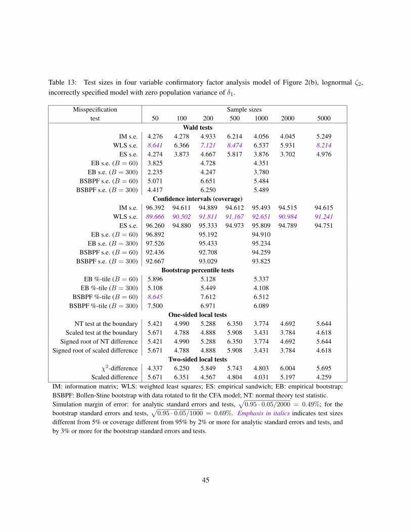
Table 13: Test sizes in four variable confirmatory factor analysis model of Figure 2(b), lognormal ζ2,incorrectly specified model with zero population variance of δ1.

Misspecification Sample sizestest 50 100 200 500 1000 2000 5000

Wald testsIM s.e. 4.276 4.278 4.933 6.214 4.056 4.045 5.249

WLS s.e. 8.641 6.366 7.121 8.474 6.537 5.931 8.214ES s.e. 4.274 3.873 4.667 5.817 3.876 3.702 4.976

EB s.e. (B = 60) 3.825 4.728 4.351EB s.e. (B = 300) 2.235 4.247 3.780

BSBPF s.e. (B = 60) 5.071 6.651 5.484BSBPF s.e. (B = 300) 4.417 6.250 5.489

Confidence intervals (coverage)IM s.e. 96.392 94.611 94.889 94.612 95.493 94.515 94.615

WLS s.e. 89.666 90.502 91.811 91.167 92.651 90.984 91.241ES s.e. 96.260 94.880 95.333 94.973 95.809 94.789 94.751

EB s.e. (B = 60) 96.892 95.192 94.910EB s.e. (B = 300) 97.526 95.433 95.234

BSBPF s.e. (B = 60) 92.436 92.708 94.259BSBPF s.e. (B = 300) 92.667 93.029 93.825

Bootstrap percentile testsEB %-tile (B = 60) 5.896 5.128 5.337

EB %-tile (B = 300) 5.108 5.449 4.108BSBPF %-tile (B = 60) 8.645 7.612 6.512

BSBPF %-tile (B = 300) 7.500 6.971 6.089One-sided local tests

NT test at the boundary 5.421 4.990 5.288 6.350 3.774 4.692 5.644Scaled test at the boundary 5.671 4.788 4.888 5.908 3.431 3.784 4.618

Signed root of NT difference 5.421 4.990 5.288 6.350 3.774 4.692 5.644Signed root of scaled difference 5.671 4.788 4.888 5.908 3.431 3.784 4.618

Two-sided local testsχ2-difference 4.337 6.250 5.849 5.743 4.803 6.004 5.695

Scaled difference 5.671 6.351 4.567 4.804 4.031 5.197 4.259IM: information matrix; WLS: weighted least squares; ES: empirical sandwich; EB: empirical bootstrap;BSBPF: Bollen-Stine bootstrap with data rotated to fit the CFA model; NT: normal theory test statistic.Simulation margin of error: for analytic standard errors and tests,

√0.95 · 0.05/2000 = 0.49%; for the

bootstrap standard errors and tests,√

0.95 · 0.05/1000 = 0.69%. Emphasis in italics indicates test sizesdifferent from 5% or coverage different from 95% by 2% or more for analytic standard errors and tests, andby 3% or more for the bootstrap standard errors and tests.

45

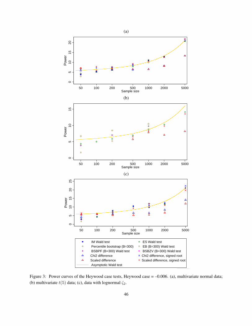
(a)

05

1015

20

50 100 200 500 1000 2000 5000Sample size

IM Wald test ES Wald test Percentile bootstrap (B=300) EB (B=300) Wald test BSBPF (B=300) Wald test BSBZV (B=300) Wald test Chi2 difference Chi2 difference, signed rootScaled difference Scaled difference, signed root Asymptotic Wald test

Pow

er

(b)

05

1015

50 100 200 500 1000 2000 5000Sample size

Asymptotic Wald test ES Wald test Percentile bootstrap (B=300) EB (B=300) Wald test BSBPF (B=300) Wald test BSBZV (B=300) Wald test Scaled difference Scaled difference, signed root

Pow

er

(c)

05

1015

2025

50 100 200 500 1000 2000 5000Sample size

IM Wald test ES Wald test Percentile bootstrap (B=300) EB (B=300) Wald test BSBPF (B=300) Wald test BSBZV (B=300) Wald test Chi2 difference Chi2 difference, signed rootScaled difference Scaled difference, signed root Asymptotic Wald test

Pow

er0

510

1520

25

50 100 200 500 1000 2000 5000Sample size

IM Wald test ES Wald test Percentile bootstrap (B=300) EB (B=300) Wald test BSBPF (B=300) Wald test BSBZV (B=300) Wald test Chi2 difference Chi2 difference, signed rootScaled difference Scaled difference, signed root Asymptotic Wald test

Pow

er

Figure 3: Power curves of the Heywood case tests, Heywood case = –0.006. (a), multivariate normal data;(b) multivariate t(5) data; (c), data with lognormal ζ2.

46

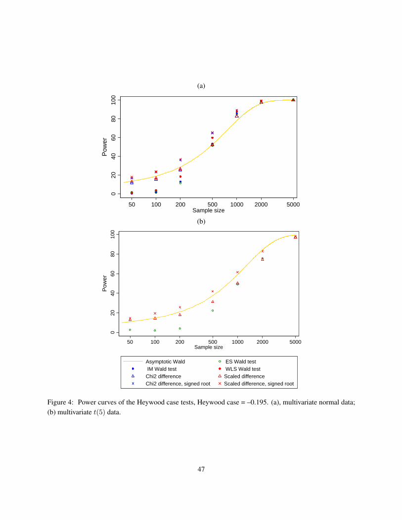
(a)

020

4060

8010

0

50 100 200 500 1000 2000 5000Sample size

Asymptotic Wald IM Wald test SB Wald test Chi2 differenceChi2 difference, signed root Scaled differenceScaled difference, signed root ES Wald test

Pow

er

(b)

020

4060

8010

0

50 100 200 500 1000 2000 5000Sample size

ES Wald test Scaled differenceScaled difference, signed root WaldPt5

Pow

er0

2040

6080

100

50 100 200 500 1000 2000 5000Sample size

Asymptotic Wald ES Wald test IM Wald test WLS Wald testChi2 difference Scaled differenceChi2 difference, signed root Scaled difference, signed root

Pow

er

Figure 4: Power curves of the Heywood case tests, Heywood case = –0.195. (a), multivariate normal data;(b) multivariate t(5) data.

47

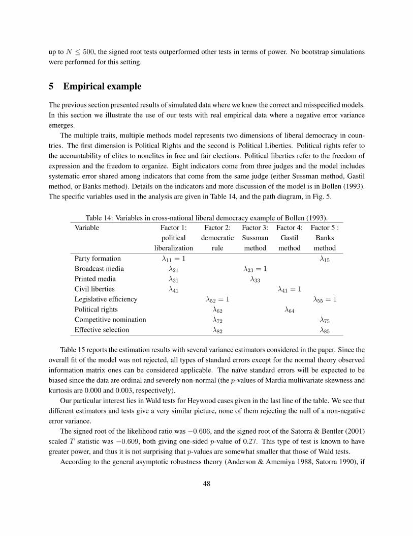
up to N ≤ 500, the signed root tests outperformed other tests in terms of power. No bootstrap simulationswere performed for this setting.

5 Empirical example

The previous section presented results of simulated data where we knew the correct and misspecified models.In this section we illustrate the use of our tests with real empirical data where a negative error varianceemerges.

The multiple traits, multiple methods model represents two dimensions of liberal democracy in coun-tries. The first dimension is Political Rights and the second is Political Liberties. Political rights refer tothe accountability of elites to nonelites in free and fair elections. Political liberties refer to the freedom ofexpression and the freedom to organize. Eight indicators come from three judges and the model includessystematic error shared among indicators that come from the same judge (either Sussman method, Gastilmethod, or Banks method). Details on the indicators and more discussion of the model is in Bollen (1993).The specific variables used in the analysis are given in Table 14, and the path diagram, in Fig. 5.

Table 14: Variables in cross-national liberal democracy example of Bollen (1993).Variable Factor 1: Factor 2: Factor 3: Factor 4: Factor 5 :

political democratic Sussman Gastil Banksliberalization rule method method method

Party formation λ11 = 1 λ15

Broadcast media λ21 λ23 = 1Printed media λ31 λ33

Civil liberties λ41 λ41 = 1Legislative efficiency λ52 = 1 λ55 = 1Political rights λ62 λ64

Competitive nomination λ72 λ75

Effective selection λ82 λ85

Table 15 reports the estimation results with several variance estimators considered in the paper. Since theoverall fit of the model was not rejected, all types of standard errors except for the normal theory observedinformation matrix ones can be considered applicable. The naıve standard errors will be expected to bebiased since the data are ordinal and severely non-normal (the p-values of Mardia multivariate skewness andkurtosis are 0.000 and 0.003, respectively).

Our particular interest lies in Wald tests for Heywood cases given in the last line of the table. We see thatdifferent estimators and tests give a very similar picture, none of them rejecting the null of a non-negativeerror variance.

The signed root of the likelihood ratio was −0.606, and the signed root of the Satorra & Bentler (2001)scaled T statistic was −0.609, both giving one-sided p-value of 0.27. This type of test is known to havegreater power, and thus it is not surprising that p-values are somewhat smaller that those of Wald tests.

According to the general asymptotic robustness theory (Anderson & Amemiya 1988, Satorra 1990), if

48

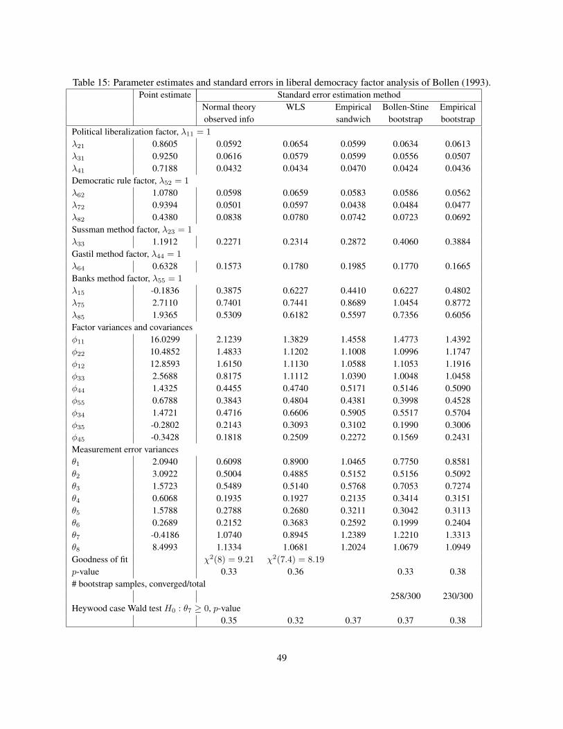
Table 15: Parameter estimates and standard errors in liberal democracy factor analysis of Bollen (1993).Point estimate Standard error estimation method

Normal theory WLS Empirical Bollen-Stine Empiricalobserved info sandwich bootstrap bootstrap

Political liberalization factor, λ11 = 1λ21 0.8605 0.0592 0.0654 0.0599 0.0634 0.0613λ31 0.9250 0.0616 0.0579 0.0599 0.0556 0.0507λ41 0.7188 0.0432 0.0434 0.0470 0.0424 0.0436Democratic rule factor, λ52 = 1λ62 1.0780 0.0598 0.0659 0.0583 0.0586 0.0562λ72 0.9394 0.0501 0.0597 0.0438 0.0484 0.0477λ82 0.4380 0.0838 0.0780 0.0742 0.0723 0.0692Sussman method factor, λ23 = 1λ33 1.1912 0.2271 0.2314 0.2872 0.4060 0.3884Gastil method factor, λ44 = 1λ64 0.6328 0.1573 0.1780 0.1985 0.1770 0.1665Banks method factor, λ55 = 1λ15 -0.1836 0.3875 0.6227 0.4410 0.6227 0.4802λ75 2.7110 0.7401 0.7441 0.8689 1.0454 0.8772λ85 1.9365 0.5309 0.6182 0.5597 0.7356 0.6056Factor variances and covariancesφ11 16.0299 2.1239 1.3829 1.4558 1.4773 1.4392φ22 10.4852 1.4833 1.1202 1.1008 1.0996 1.1747φ12 12.8593 1.6150 1.1130 1.0588 1.1053 1.1916φ33 2.5688 0.8175 1.1112 1.0390 1.0048 1.0458φ44 1.4325 0.4455 0.4740 0.5171 0.5146 0.5090φ55 0.6788 0.3843 0.4804 0.4381 0.3998 0.4528φ34 1.4721 0.4716 0.6606 0.5905 0.5517 0.5704φ35 -0.2802 0.2143 0.3093 0.3102 0.1990 0.3006φ45 -0.3428 0.1818 0.2509 0.2272 0.1569 0.2431Measurement error variancesθ1 2.0940 0.6098 0.8900 1.0465 0.7750 0.8581θ2 3.0922 0.5004 0.4885 0.5152 0.5156 0.5092θ3 1.5723 0.5489 0.5140 0.5768 0.7053 0.7274θ4 0.6068 0.1935 0.1927 0.2135 0.3414 0.3151θ5 1.5788 0.2788 0.2680 0.3211 0.3042 0.3113θ6 0.2689 0.2152 0.3683 0.2592 0.1999 0.2404θ7 -0.4186 1.0740 0.8945 1.2389 1.2210 1.3313θ8 8.4993 1.1334 1.0681 1.2024 1.0679 1.0949Goodness of fit χ2(8) = 9.21 χ2(7.4) = 8.19p-value 0.33 0.36 0.33 0.38# bootstrap samples, converged/total

258/300 230/300Heywood case Wald test H0 : θ7 ≥ 0, p-value

0.35 0.32 0.37 0.37 0.38

49

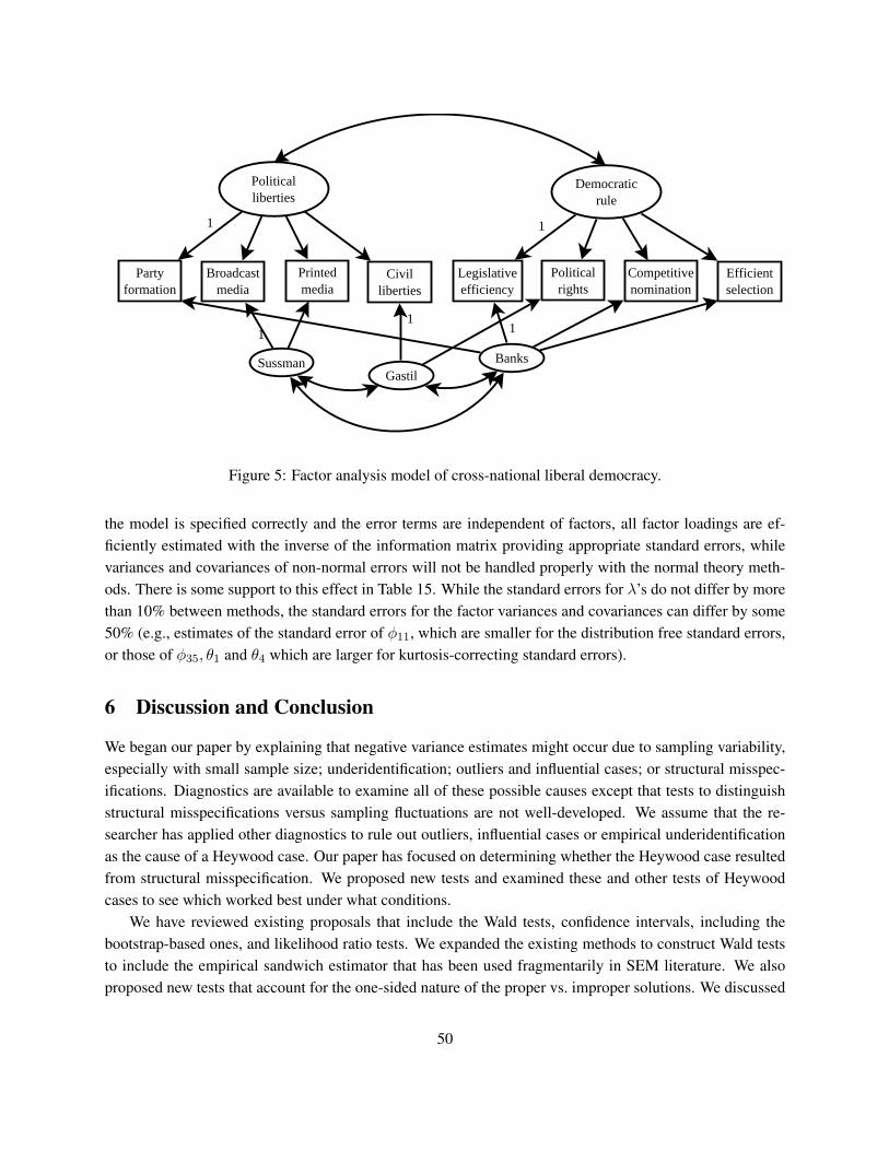
Partyformation

Broadcastmedia

Printedmedia

Civilliberties

Legislativeefficiency

Politicalrights

Competitivenomination

Efficientselection

Politicalliberties

Democraticrule

SussmanGastil

Banks

1

11

1

1

Figure 5: Factor analysis model of cross-national liberal democracy.

the model is specified correctly and the error terms are independent of factors, all factor loadings are ef-ficiently estimated with the inverse of the information matrix providing appropriate standard errors, whilevariances and covariances of non-normal errors will not be handled properly with the normal theory meth-ods. There is some support to this effect in Table 15. While the standard errors for λ’s do not differ by morethan 10% between methods, the standard errors for the factor variances and covariances can differ by some50% (e.g., estimates of the standard error of φ11, which are smaller for the distribution free standard errors,or those of φ35, θ1 and θ4 which are larger for kurtosis-correcting standard errors).

6 Discussion and Conclusion

We began our paper by explaining that negative variance estimates might occur due to sampling variability,especially with small sample size; underidentification; outliers and influential cases; or structural misspec-ifications. Diagnostics are available to examine all of these possible causes except that tests to distinguishstructural misspecifications versus sampling fluctuations are not well-developed. We assume that the re-searcher has applied other diagnostics to rule out outliers, influential cases or empirical underidentificationas the cause of a Heywood case. Our paper has focused on determining whether the Heywood case resultedfrom structural misspecification. We proposed new tests and examined these and other tests of Heywoodcases to see which worked best under what conditions.

We have reviewed existing proposals that include the Wald tests, confidence intervals, including thebootstrap-based ones, and likelihood ratio tests. We expanded the existing methods to construct Wald teststo include the empirical sandwich estimator that has been used fragmentarily in SEM literature. We alsoproposed new tests that account for the one-sided nature of the proper vs. improper solutions. We discussed

50

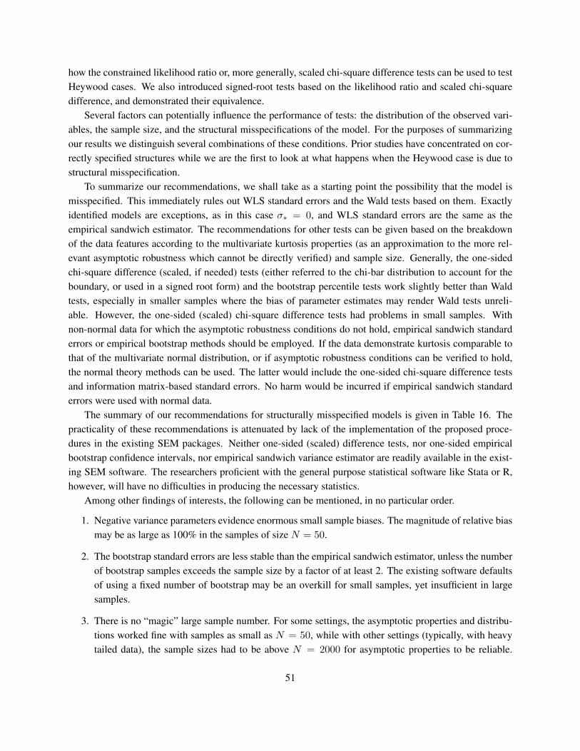
how the constrained likelihood ratio or, more generally, scaled chi-square difference tests can be used to testHeywood cases. We also introduced signed-root tests based on the likelihood ratio and scaled chi-squaredifference, and demonstrated their equivalence.

Several factors can potentially influence the performance of tests: the distribution of the observed vari-ables, the sample size, and the structural misspecifications of the model. For the purposes of summarizingour results we distinguish several combinations of these conditions. Prior studies have concentrated on cor-rectly specified structures while we are the first to look at what happens when the Heywood case is due tostructural misspecification.

To summarize our recommendations, we shall take as a starting point the possibility that the model ismisspecified. This immediately rules out WLS standard errors and the Wald tests based on them. Exactlyidentified models are exceptions, as in this case σ∗ = 0, and WLS standard errors are the same as theempirical sandwich estimator. The recommendations for other tests can be given based on the breakdownof the data features according to the multivariate kurtosis properties (as an approximation to the more rel-evant asymptotic robustness which cannot be directly verified) and sample size. Generally, the one-sidedchi-square difference (scaled, if needed) tests (either referred to the chi-bar distribution to account for theboundary, or used in a signed root form) and the bootstrap percentile tests work slightly better than Waldtests, especially in smaller samples where the bias of parameter estimates may render Wald tests unreli-able. However, the one-sided (scaled) chi-square difference tests had problems in small samples. Withnon-normal data for which the asymptotic robustness conditions do not hold, empirical sandwich standarderrors or empirical bootstrap methods should be employed. If the data demonstrate kurtosis comparable tothat of the multivariate normal distribution, or if asymptotic robustness conditions can be verified to hold,the normal theory methods can be used. The latter would include the one-sided chi-square difference testsand information matrix-based standard errors. No harm would be incurred if empirical sandwich standarderrors were used with normal data.

The summary of our recommendations for structurally misspecified models is given in Table 16. Thepracticality of these recommendations is attenuated by lack of the implementation of the proposed proce-dures in the existing SEM packages. Neither one-sided (scaled) difference tests, nor one-sided empiricalbootstrap confidence intervals, nor empirical sandwich variance estimator are readily available in the exist-ing SEM software. The researchers proficient with the general purpose statistical software like Stata or R,however, will have no difficulties in producing the necessary statistics.

Among other findings of interests, the following can be mentioned, in no particular order.

1. Negative variance parameters evidence enormous small sample biases. The magnitude of relative biasmay be as large as 100% in the samples of size N = 50.

2. The bootstrap standard errors are less stable than the empirical sandwich estimator, unless the numberof bootstrap samples exceeds the sample size by a factor of at least 2. The existing software defaultsof using a fixed number of bootstrap may be an overkill for small samples, yet insufficient in largesamples.

3. There is no “magic” large sample number. For some settings, the asymptotic properties and distribu-tions worked fine with samples as small as N = 50, while with other settings (typically, with heavytailed data), the sample sizes had to be above N = 2000 for asymptotic properties to be reliable.

51

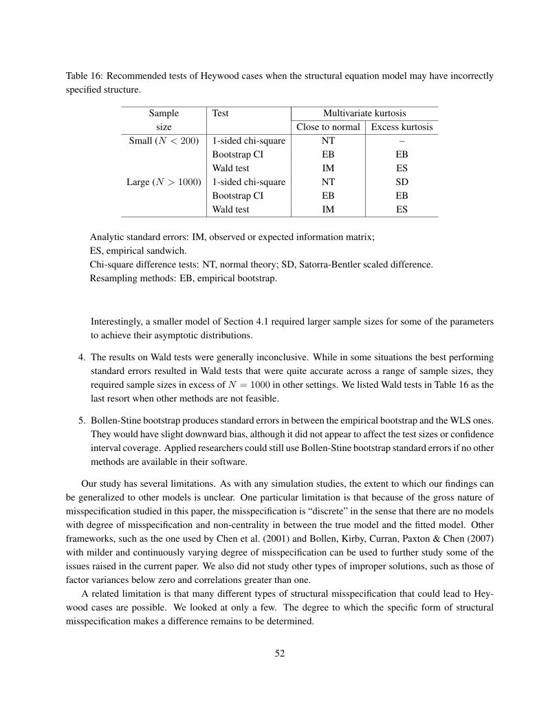
Table 16: Recommended tests of Heywood cases when the structural equation model may have incorrectlyspecified structure.

Sample Test Multivariate kurtosissize Close to normal Excess kurtosis

Small (N < 200) 1-sided chi-square NT –Bootstrap CI EB EBWald test IM ES

Large (N > 1000) 1-sided chi-square NT SDBootstrap CI EB EBWald test IM ES

Analytic standard errors: IM, observed or expected information matrix;ES, empirical sandwich.Chi-square difference tests: NT, normal theory; SD, Satorra-Bentler scaled difference.Resampling methods: EB, empirical bootstrap.

Interestingly, a smaller model of Section 4.1 required larger sample sizes for some of the parametersto achieve their asymptotic distributions.

4. The results on Wald tests were generally inconclusive. While in some situations the best performingstandard errors resulted in Wald tests that were quite accurate across a range of sample sizes, theyrequired sample sizes in excess of N = 1000 in other settings. We listed Wald tests in Table 16 as thelast resort when other methods are not feasible.

5. Bollen-Stine bootstrap produces standard errors in between the empirical bootstrap and the WLS ones.They would have slight downward bias, although it did not appear to affect the test sizes or confidenceinterval coverage. Applied researchers could still use Bollen-Stine bootstrap standard errors if no othermethods are available in their software.

Our study has several limitations. As with any simulation studies, the extent to which our findings canbe generalized to other models is unclear. One particular limitation is that because of the gross nature ofmisspecification studied in this paper, the misspecification is “discrete” in the sense that there are no modelswith degree of misspecification and non-centrality in between the true model and the fitted model. Otherframeworks, such as the one used by Chen et al. (2001) and Bollen, Kirby, Curran, Paxton & Chen (2007)with milder and continuously varying degree of misspecification can be used to further study some of theissues raised in the current paper. We also did not study other types of improper solutions, such as those offactor variances below zero and correlations greater than one.

A related limitation is that many different types of structural misspecification that could lead to Hey-wood cases are possible. We looked at only a few. The degree to which the specific form of structuralmisspecification makes a difference remains to be determined.

52

The results of our paper suggest that researchers should look for methods to improve proposed sandwichestimator’s finite sample performance. The performance of this estimator has been studied extensively inthe context of heteroskedastic regression models (Eicker 1967, White 1980, Carroll et al. 1998, Kauermann& Carroll 2001, Bera, Suprayitno & Premaratne 2002, Hardin 2003) where the small sample biases havebeen established both analytically and by simulation. This literature relies on the special linear structuresand unbiased estimation of the residual variance, which is unlikely to be directly generalizable to SEM.

The version of the information matrix estimator that we used was observed information matrix. Whileit can be conjectured that the expected information matrix will produce less accurate results under structuralmisspecification, we do not have solid evidence on this issue.

Even considering these limitations, our research provides several alternative methods to test whether anegative error variance is a symptom of structural misspecificaiton.

References

Amemiya, T. (1985), Advanced Econometrics, Harvard University Press, Cambridge, MA, USA.

Anderson, J. C. & Gerbing, D. (1984), ‘The effect of sampling error on convergence, improper solutions, andgoodness-of-fit indices for maximum likelihood confirmatory factor analysis’, Psychometrika 49, 155–173.

Anderson, T. W. & Amemiya, Y. (1988), ‘The asymptotic normal distribution of estimators in factor analysisunder general conditions’, 16(2), 759–771.

Andrews, D. F. (2007), ‘Robust likelihood inference for public policy’, The Canadian Journal of Statistics35(3), 341–350.

Andrews, D. W. K. (1999), ‘Estimation when a parameter is on a boundary’, Econometrica 67(6), 1341–1383.

Andrews, D. W. K. (2001), ‘Testing when a parameter is on the boundary of the maintained hypothesis’,Econometrica 69(3), 683–734. doi:10.1111/1468-0262.00210.

Arbuckle, J. (1997), AMOS Users Guide: Version 3.6, SmallWaters, Chicago.

Arminger, G. & Schoenberg, R. J. (1989), ‘Pseudo maximum likelihood estimation and a test for misspeci-fication in mean and covariance structure models’, Psychometrika 54, 409–426.

Barndorff-Nielsen, O. E. & Cox, D. R. (1994), Inference and Asymptotics, Monographs on Statistics andApplied Probability, Chapman & Hall/CRC, New York.

Bera, A. K., Suprayitno, T. & Premaratne, G. (2002), ‘On some heteroskedasticity-robust estimators ofvariance-covariance matrix of the least-squares estimators’, Journal of Statistical Planning and Infer-ence 108(1–2), 121–136.

Beran, R. & Srivastava, M. S. (1985), ‘Bootstrap tests and confidence regions for functions of a covariancematrix’, The Annals of Statistics 13(1), 95–115.

53

Berndt, E., Hall, B., Hall, R. & Hausman, J. (1974), ‘Estimation and inference in nonlinear structuralmodels’, Annals of Economic and Social Measurement 3/4, 653–665.

Binder, D. A. (1983), ‘On the variances of asymptotically normal estimators from complex surveys’, Inter-national Statistical Review 51, 279–292.

Bollen, K. (1993), ‘Liberal democracy: Validity and method factors in cross-national measures’, AmericanJournal of Political Science 37(4), 1207–1230.

Bollen, K. A. (1987), ‘Outliers and improper solutions: A confirmatory factor analysis example’, Sociolog-ical Methods and Research 15, 375–384.

Bollen, K. A. (1989), Structural Equations with Latent Variables, Wiley, New York.

Bollen, K. A. (1996a), ‘An alternative two stage least squares (2SLS) estimator for latent variable models’,Psychometrika 61(1), 109–121.

Bollen, K. A. (1996b), A limited-information estimator for LISREL models with and without heteroscedas-tic errors, in G. Marcoulides & R. Schumaker, eds, ‘Advanced Structural Equation Modeling Tech-niques’, Erlbaum, Mahwah, NJ, pp. 227–241.

Bollen, K. A. & Arminger, G. (1991), ‘Observational residuals in factor analysis and structural equationmodels’, Sociological Methodology 21, 235–262.

Bollen, K. A., Kirby, J. B., Curran, P. J., Paxton, P. M. & Chen, F. (2007), ‘Latent variable models under mis-specification: two-stage least squares (2SLS) and maximum likelihood (ML) estimators’, SociologicalMethods and Research 36(1), 48–86.

Bollen, K. & Stine, R. (1992), ‘Bootstrapping goodness of fit measures in structural equation models’,Sociological Methods and Research 21, 205–229.

Boomsma, A. (1983), On the Robustness of LISREL (Maximum Likelihood Estimation) Against Small Sam-ple Size and Nonnormality, Sociometric Research Foundation, Amsterdam, the Netherlands.

Boomsma, A. & Hoogland, J. J. (2001), ‘The robustness of LISREL modeling revisited’, Structural EquationModeling: Present and Future.

Browne, M. W. (1984), ‘Asymptotically distribution-free methods for the analysis of the covariance struc-tures’, British Journal of Mathematical and Statistical Psychology 37, 62–83.

Buse, A. (1982), ‘The likelihood ratio, Wald, and Lagrange multiplier tests: An expository note’, TheAmerican Statistician 36(3), 153–157.

Cadigan, N. G. (1995), ‘Local influence in structural equation models’, Structural Equation Modeling 2, 13–30.

Canty, A. J., Davison, A. C., Hinkley, D. V. & Ventura, V. (2006), ‘Bootstrap diagnostics and remedies’, TheCanadian Journal of Statistics/La revue canadienne de statistique 34(1), 5–27.

54

Carroll, R. J., Wang, S., Simpson, D. G., Stromberg, A. J. & Ruppert, D. (1998), The sandwich (robustcovariance matrix) estimator, Technical report, Deparment of Statistics, Texas A & M University,College Station, TX. Available at http://www.stat.tamu.edu/ftp/pub/rjcarroll/sandwich.pdf.

Chen, F., Bollen, K. A., Paxton, P., Curran, P. & Kirby, J. (2001), ‘Improper solutions in structural equationmodels: Causes, consequences, and strategies’, Sociological Methods and Research 25, 223–251.

Chernoff, H. (1954), ‘On the distribution of the likelihood ratio’, The Annals of Mathematical Statistics25(3), 573–578.

Davidson, R. & MacKinnon, J. (1993), Estimation and Inference in Econometrics, Oxford University Press,New York.

Dillon, W. R., Kumar, A. & Mulani, N. (1987), ‘Offending estimates in covariance structure analysis: Com-ments on the causes and solutions to Heywood cases’, Psychological Bulletin 101, 126–135.

Efron, B. (1979), ‘Bootstrap methods: Another look at the jackknife’, Annals of Statistics 7, 1–26.

Efron, B. & Tibshirani, R. J. (1994), An Introduction to the Bootstrap, Chapman & Hall/CRC.

Eicker, F. (1967), Limit theorems for regressions with unequal and dependent errors, in ‘Proceedings of theFifth Berkeley Symposium on Mathematical Statistics and Probability’, Vol. 1, University of CaliforniaPress, Berkeley, pp. 59–82.

Ferguson, T. S. (1996), A Course in Large Sample Theory, Texts in Statistical Science, Chapman &Hall/CRC, London.

Fletcher, R. (1980), Practical Methods of Optimization, Wiley Interscience, New York.

Gonzalez, R. & Griffin, D. (2001), ‘Testing parameters in structural equation modeling: Every ”one” mat-ters.’, Psychological Methods 6(3), 258–269.

Gould, W., Pittblado, J. & Sribney, W. (2006), Maximum Likelihood Estimation with Stata, 3rd edn, StataPress, College Station, TX.

Hall, P. (1992), The Bootstrap and Edgeworth Expansion, Springer Series in Statistics, Springer, New York.

Hardin, J. W. (2003), The sandwich estimator of variance, in T. B. Fomby & R. C. Hill, eds, ‘MaximumLikelihood Estimation of Misspecified Models: Twenty Years Later’, Elsevier, New York.

Heywood, H. B. (1931), ‘On finite sequences of real numbers’, Proceedings of the Royal Society of London.Series A, Containing Papers of a Mathematical and Physical Character 134(824), 486–501.

Huber, P. (1967), The behavior of the maximum likelihood estimates under nonstandard conditions, in‘Proceedings of the Fifth Berkeley Symposium on Mathematical Statistics and Probability’, Vol. 1,University of California Press, Berkeley, pp. 221–233.

Huber, P. (1974), Robust Statistics, Wiley, New York.

55

Jennrich, R. (2008), ‘Nonparametric estimation of standard errors in covariance analysis using the infinites-imal jackknife’, Psychometrika 73(4), 579–594.

Joreskog, K. G. (1978), ‘Structural analysis of covariance and correlation matrices’, Psychometrika 43, 443–477.

Kauermann, G. & Carroll, R. J. (2001), ‘A note on the efficiency of sandwich covariance matrix estimation’,Journal of the American Statistical Association 96(456), 1387–1396.

Kolenikov, S. (2009), ‘Confirmatory factor analysis with confa’, Stata Journal 9(3), 329–373.

Kovar, J. G., Rao, J. N. K. & Wu, C. F. J. (1988), ‘Bootstrap and other methods to measure errors in surveyestimates’, Canadian Journal of Statistics 16, 25–45.

Kudo, A. (1963), ‘A multivariate analogue of the one-sided test’, Biometrika 50(3 and 4), 403–418.

Lafontaine, F. & White, K. J. (1986), ‘Obtaining any Wald statistic you want’, Economics Letters 21, 35–40.

Lee, S. & Jennrich, R. (1979), ‘A study of algorithms for covariance structure analysis with specific com-parisons using factor analysis’, Psychometrika 44(1), 99–113.

Magnus, J. R. & Neudecker, H. (1999), Matrix calculus with applications in statistics and econometrics,2nd edn, John Wiley & Sons.

Moustaki, I. & Victoria-Feser, M.-P. (2006), ‘Bounded influence robust estimation in generalized linearlatent variable models’, Journal of the American Statistical Association 101(474), 644–653. DOI10.1198/016214505000001320.

Muthen, B. O. & Satorra, A. (1995), ‘Complex sample data in structural equation modeling’, SociologicalMethodology 25, 267–316.

Neudecker, H. & Satorra, A. (1991), ‘Linear structural relations: Gradient and Hessian of the fitting func-tion’, Statistics and Probability Letters 11, 57–61.

Perlman, M. D. (1969), ‘One-sided testing problems in multivariate analysis’, The Annals of MathematicalStatistics 40(2), 549–567.

Phillips, P. C. B. & Park, J. Y. (1988), ‘On the formulation of Wald tests of nonlinear restrictions’, Econo-metrica 56, 1065–1083.

Rabe-Hesketh, S. & Skrondal, A. (2005), Multilevel and Longitudinal Modeling Using Stata, Stata Press,College Station, TX.

Rabe-Hesketh, S., Skrondal, A. & Pickles, A. (2004), ‘Generalized multilevel structural equation modeling’,Psychometrika 69(2), 167–190.

Rindskopf, D. (1984), ‘Structural equation models: Empirical identification, Heywood cases, and relatedproblems’, Sociological Methods and Research 13, 109–119.

56

Sato, M. (1987), ‘Pragmatic treatment of improper solutions in factor analysis’, Annals of the Institute ofStatistics and Mathematics, part B 39, 443–455.

Satorra, A. (1990), ‘Robustness issues in structural equation modeling: A review of recent developments’,Quality and Quantity 24, 367–386.

Satorra, A. (1992), ‘Asymptotic robust inference in the analysis of mean and covariance structures’, Socio-logical Methodology 22, 249–278.

Satorra, A. & Bentler, P. (2001), ‘A scaled difference chi-square test statistic for moment structure analysis’,Psychometrika 66(4), 507–514.

Satorra, A. & Bentler, P. M. (1990), ‘Model conditions for asymptotic robustness in the analysis oflinear relations’, Computational Statistics and Data Analysis 10(3), 235–249. doi:10.1016/0167-9473(90)90004-2.

Satorra, A. & Bentler, P. M. (1994), Corrections to test statistics and standard errors in covariance structureanalysis, in A. von Eye & C. C. Clogg, eds, ‘Latent variables analysis’, Sage, Thousands Oaks, CA,pp. 399–419.

Savalei, V. (forthcoming), ‘Expected vs. observed information in SEM with incomplete normal and nonnor-mal data’, Psychological Methods .

Savalei, V. & Kolenikov, S. (2008), ‘Constrained vs. unconstrained estimation in structural equation model-ing’, Psychological Methods 13, 150–170.

Shao, J. & Tu, D. (1995), The Jackknife and Bootstrap, Springer, New York.

Shapiro, A. (1985), ‘Asymptotic distribution of test statistic in the analysis of moment structures underinequality constraints’, Biometrika 72(1), 133–144.

Shapiro, A. (1988), ‘Towards a unified theory of inequality constrained testing in multivariate analysis’,International Statistical Review 56(1), 49–62.

Skinner, C. J. (1989), Domain means, regression and multivariate analysis, in C. J. Skinner, D. Holt & T. M.Smith, eds, ‘Analysis of Complex Surveys’, Wiley, New York, chapter 3, pp. 59–88.

Skrondal, A. (2000), ‘Design and analysis of Monte Carlo experiments: Attacking the conventional wis-dom’, Multivariate Behavioral Research 35(2), 137–167.

Skrondal, A. & Rabe-Hesketh, S. (2004), Generalized Latent Variable Modeling, Chapman and Hall/CRC,Boca Raton, Florida.

Stata Corp. (2007), Stata Statistical Software: Release 10, College Station, TX, USA.

Stoel, R. D., Garre, F. G., Dolan, C. & van den Wittenboer, G. (2006), ‘On the likelihood ratio test instructural equation modeling when parameters are subject to boundary constraints’, PsychologicalMethods 11(4).

57

van der Vaart, A. W. (1998), Asymptotic Statistics, Cambridge University Press, Cambridge.

Van Driel, O. P. (1978), ‘On various causes of improper solutions in maximum likelihood factor analysis’,Psychometrika 43, 225–43.

West, K. D. & Newey, W. K. (1987), ‘A simple, positive semi-definite, heteroskedasticity and autocorrelationconsistent covariance matrix’, Econometrica 55(3), 703–708.

White, H. (1980), ‘A heteroskedasticity-consistent covariance-matrix estimator and a direct test for het-eroskedasticity’, Econometrica 48(4), 817–838.

White, H. (1982), ‘Maximum likelihood estimation of misspecified models’, Econometrica 50(1), 1–26.

White, H. (1996), Estimation, Inference and Specification Analysis, Vol. 22 of Econometric Society Mono-graphs, Cambridge University Press, New York.

Yuan, K.-H. & Bentler, P. M. (1997), ‘Mean and covariance structure analysis: Theoretical and practicalimprovements’, Journal of the American Statistical Association 92(438), 767–774.

Yuan, K.-H. & Bentler, P. M. (2007), Structural equation modeling, in C. Rao & S. Sinharay, eds, ‘Handbookof Statistics: Psychometrics’, Vol. 26 of Handbook of Statistics, Elsevier, chapter 10.

Yuan, K.-H. & Chan, W. (2005), ‘On nonequivalence of several procedures of structural equation modeling’,Psychometrika 70(4), 791–798.

Yuan, K.-H. & Hayashi, K. (2006), ‘Standard errors in covariance structure models: Asymptotics versusbootstrap’, British Journal of Mathematical and Statistical Psychology 59, 397–417.

Appendices

A Numeric maximization, derivatives, and the sandwich estimator

This appendix provides basic information about numeric likelihood maximization procedures, the numericderivatives that are obtained as a part of that procedure, and combining those derivatives into the sandwichestimator. Exposition is based on Gould et al. (2006), using their notation, and is oriented at implementationin Stata software (Stata Corp. 2007).

While analytic derivatives tend to lead to faster and more accurate algorithms, the numeric derivativesare very general and require no derivations and specialized coding, and they are easier to generalize forother estimation problems, such as complex survey designs (Muthen & Satorra 1995). This approach iscloser in spirit to GLLAMM estimation procedures (Rabe-Hesketh et al. 2004, Skrondal & Rabe-Hesketh2004, Rabe-Hesketh & Skrondal 2005) than to traditional LISREL-type algorithms relying on manipulationof the moment matrices. Both approaches use (24) (or equivalently (10a) and (10b) of Yuan & Hayashi(2006)), but provide different implementations of the resulting estimators. Yuan & Hayashi (2006) take thisestimator as a starting point, and further pursue the necessary first and second derivatives of the likelihood

58

to obtain explicit matrix expressions that would involve the estimated parameters and their functions (suchas implied moment matrices and their derivatives), as well as the third and the fourth moments of the data.

The usual preference for analytical computations may not always be warranted. For larger models,computations of the fourth order moments matrix in either Satorra-Bentler or Yuan-Hayashi estimatorswill require O(np4) operations, with additional slow element-by-element operations for the derivatives ofthe moment conditions. The computations of the matrices A, B in the empirical version of the sandwichestimator will require O(nt2) operations where t is the number of parameters to be estimated. If the numberof parameters is roughly proportional to the number of observed variables (and in most SEMs, each observedvariable would require at least one loading and the variance parameter), the analytical derivatives might takelonger to compute.

Suppose the sample observations Xi are i.i.d. coming from distribution f(x, θ) where f(·) is the density(or, in some discrete problems, the probability density function). Then the maximum likelihood estimationproblem consists of finding the solution of

ln l(θ,X) =n∑i=1

ln f(xi, θ)→ maxθ

(53)

The typical SEM example combines assumptions about the model structure to obtain the parameterizedmean and covariance matrices as in (5) with the assumption of multivariate normality to obtain the likeli-hood. In the common situation that the above problem cannot be solved analytically, an iterative maximiza-tion algorithm has to be set up. The most popular class of algorithms are those based on Newton-Raphsoniterations:

1. Start with the initial values of θ1, obtained from a random search, another estimation routine, suppliedby user, etc.

2. Compute the derivatives of the objective function:

g(θ) =∂

∂θln l(θ,X)

H(θ) =∂2

∂θ ∂θ′ln l(θ,X) (54)

3. Determine the direction of the next step d = −[H(θk)

]−1g(θk)

4. Compute the next iterationθk+1 = θk + hkd (55)

where the step size hk is chosen to make an improvement of the objective function along direction d.

5. Check convergence criteria (usually of the form ‖g(θk)‖ < ε for some small ε ∼ 10−6); if satisfied,stop; if not, return to step 2.

59

The above algorithm needs the first and second derivatives, g(θk) andH(θk). If those are not availablefrom the likelihood program, Stata can compute them numerically. The derivatives are approximated as

f ′(z) ≈ f(z + d2)− f(z − d

2)d

,

f ′′(z) ≈ f(z + d)− f(z) + f(z − d)− f(z)d2

, (56)

(57)

where the step size d is computed so that f(z) and f(z ± d) differ in about half their digits. Thus if f , thelog-likelihood function, is computed in double arithmetics with 16 digits, the differences in both numeratorswill be computed with accuracy of 8 digits.

There is a number of additional smart features of Stata’s likelihood maximizer. If matrix H(θk) isdeemed non-invertible, it uses the steepest ascent algorithm where the update is performed as

θk+1 = θk − hkg(θk) (58)

It can take a compromise between the two algorithms by scaling the diagonal elements ofH(θk) to make itinvertible, and it can take a spectral decomposition ofH(θk) to identify the subspaces where the (projectionof the) likelihood is convex, and thus Newton-Raphson steps can be taken, and the orthogonal subspacewhere the (projection of the) likelihood is flat, and steepest ascent needs to be performed. Other variationsof the maximizer are choices between several options of avoiding direct computation of the H(θk) matrix:BHHH algorithm (Berndt, Hall, Hall & Hausman 1974) that replaces H(θk) by −g(θk)g(θk)′; and DFPand BFGS algorithms that build up improved approximations toH(θk) (Fletcher 1980).

It is easy to see that the above algorithms provide all the building blocks for the sandwich estimator (24).If the observation-level contributions to those matrices

gi(θ) =∂

∂θln l(θ, xi)

H i(θ) =∂2

∂θ ∂θ′ln l(θ, xi)

are provided analytically or computed numerically, then the components of the sandwich estimator areobtained as

A =1n

n∑i=1

H i(θ),

B =1n

n∑i=1

gi(θ)gi(θ)′ (59)

It is also automatically available with Stata’s robust option, implemented through the lower level robust

command that provides the computations in (59). The simplicity of implementation allows relatively straight-forward extensions to more complicated situations, such as clustered data and data coming from complexsurveys. In those situations, the summations needs to be taken over clusters, or PSUs, and the individualobservations might need to be weighted according to sampling weights.

60