terre plate, au centre du...

Terre plate, au centre du monde...

Galilée

Kepler

Christophe Colomb

Eratosthène

Descartes (1596-1650)

Gautier (1660-1737)

Jules Verne (1828-1905)

La gravimétrie

La géophysique pour étudier

la Terre et les autres planètes

La sismologie

L’électrique

La magnétotellurique La thermique

La géodésie

La gravimétrieEtude du champ de pesanteur

Information sur la répartition des masses dans les corps

Champ de pesanteur d’un ellipsoïde

Modification locale du champ

La gravimétrie

La gravimétrieAvec quoi mesure-t-on ?

➡ Un pendule (Bouguer)

➡ Un gravimètre

➡ Des satellites ...

La gravimétriePrécision de la mesureMesures de la pesanteur et de ses variations

Erreurs cumulées sur le géoïde

GOCE

HypothèseCHAMP : 7 ansGRACE : 5 ansGOCE : 1 anMesures terrestres

Mesures spatiales

La gravimétrieQu’est-ce que ça donne ?

➡ Sur Terre

➡Sur la Lune

➡Sur Mars

La gravimétriePour la Lune

ELEMENTS FEBRUARY 200937

By subtracting the gravitational contribution associated with the surface relief and mare basalts from the observed gravity field, the remaining signal can be modeled in terms of variations in relief along the crust–mantle interface, providing us with a global map of the Moon’s crustal thick-ness. One such model is shown in FIGURE 2 (lower left), which demonstrates that the crust is considerably thinned, and in some cases nearly absent, beneath the largest impact basins. This thinned crust is a natural consequence of the impact-cratering process, which is thought to excavate materials from depths of up to one-tenth of the crater’s diameter. Thus, even though all of the samples that we have from the Moon were collected on the surface, many of them could have originated tens of kilometers below the surface, perhaps even in the mantle.

Although the geophysical crustal-thickness models are invaluable for deciphering both the impact-cratering process and the provenance of the lunar samples, several vexing questions remain. For instance, the model in FIGURE 2 predicts that the crustal thickness is on average greater on the farside hemisphere than on the nearside, but this could conceivably be an artifact of the geophysical model that assumes the crustal and mantle densities are everywhere the same. In addition, even though the South Pole–Aitken basin is the largest impact structure on the Moon, this model predicts that there is still a thin “crust” in the basin’s interior. These materials could represent potentially deep crustal materials that were exposed by the impact (Pieters et al. 2001), or perhaps a differentiated impact melt sheet. Alternatively, the assumptions of the geophysical model might be inappropriate for this region of the Moon, and the mantle might be closer to the surface than is predicted. Given that this basin is the oldest recog-nizable impact structure on the Moon, it is plausible that this impact might have occurred while the crust was still forming during the terminal stages of magma-ocean crystal li zation.

THE MANTLEThe Apollo seismic data are the primary source of informa-tion bearing on the structure and composition of the lunar mantle. Events detected over the approximately eight-year operation of the Apollo seismic network included about 1800 meteoroid impacts, 28 energetic shallow moonquakes (with body wave magnitudes up to 5 and hypocenters about 100 km below the surface), and about 7000 extremely weak deep moonquakes that were located about halfway to the center of the Moon (FIGURE 3 shows the seismic ray paths as a function of epicentral distance and hypocenter depth for all stations). The deep moonquakes are very enigmatic in that their occurrences are correlated in some way with the tides raised by the Earth, they involve very low stress drops (less than 1 bar), they appear to originate from about 300 “nests” that are repeatedly activated, and almost all of these nests are located on the Moon’s nearside hemi-sphere (Nakamura 2003; Bulow et al. 2007). The nearside distribution of the deep moonquakes could perhaps indi-cate that the farside hemisphere is seismically inactive. Such a hypothesis is possible, especially if one considers that almost all of the Moon’s mare basalts erupted on its nearside hemisphere. Alternatively, it is possible that the deepest interior of the Moon attenuates seismic signals originating from farside events. In support of this hypoth-esis, shear-wave arrivals appear to be absent for those ray paths that probe the deepest portions of the mantle, perhaps indicating the presence of a partial melt in this zone (Nakamura 2005). The presence of a highly attenu-ating zone deep in the lunar mantle is also consistent with analyses of the lunar laser ranging data (these indicate a bulk solid-body “quality factor” Q of about 30, which is comparable to that of the Earth and Mars; Williams et al. 2001). One scenario that might be consistent with the

FIGURE 2 Surface relief (upper left), radial gravity (upper right; positive is directed downward), modeled crustal thick-

ness (lower left), and magnetic-field strength at 30 km altitude (low-er right). Each image consists of two Lambert azimuthal equal-area projections of the lunar near- and farside hemispheres.


By subtracting the gravitational contribution associated with the surface relief and mare basalts from the observed gravity field, the remaining signal can be modeled in terms of variations in relief along the crust–mantle interface, providing us with a global map of the Moon’s crustal thick-ness. One such model is shown in FIGURE 2 (lower left), which demonstrates that the crust is considerably thinned, and in some cases nearly absent, beneath the largest impact basins. This thinned crust is a natural consequence of the impact-cratering process, which is thought to excavate materials from depths of up to one-tenth of the crater’s diameter. Thus, even though all of the samples that we have from the Moon were collected on the surface, many of them could have originated tens of kilometers below the surface, perhaps even in the mantle.

Although the geophysical crustal-thickness models are invaluable for deciphering both the impact-cratering process and the provenance of the lunar samples, several vexing questions remain. For instance, the model in FIGURE 2 predicts that the crustal thickness is on average greater on the farside hemisphere than on the nearside, but this could conceivably be an artifact of the geophysical model that assumes the crustal and mantle densities are everywhere the same. In addition, even though the South Pole–Aitken basin is the largest impact structure on the Moon, this model predicts that there is still a thin “crust” in the basin’s interior. These materials could represent potentially deep crustal materials that were exposed by the impact (Pieters et al. 2001), or perhaps a differentiated impact melt sheet. Alternatively, the assumptions of the geophysical model might be inappropriate for this region of the Moon, and the mantle might be closer to the surface than is predicted. Given that this basin is the oldest recog-nizable impact structure on the Moon, it is plausible that this impact might have occurred while the crust was still forming during the terminal stages of magma-ocean crystal li zation.

THE MANTLEThe Apollo seismic data are the primary source of informa-tion bearing on the structure and composition of the lunar mantle. Events detected over the approximately eight-year operation of the Apollo seismic network included about 1800 meteoroid impacts, 28 energetic shallow moonquakes (with body wave magnitudes up to 5 and hypocenters about 100 km below the surface), and about 7000 extremely weak deep moonquakes that were located about halfway to the center of the Moon (FIGURE 3 shows the seismic ray paths as a function of epicentral distance and hypocenter depth for all stations). The deep moonquakes are very enigmatic in that their occurrences are correlated in some way with the tides raised by the Earth, they involve very low stress drops (less than 1 bar), they appear to originate from about 300 “nests” that are repeatedly activated, and almost all of these nests are located on the Moon’s nearside hemi-sphere (Nakamura 2003; Bulow et al. 2007). The nearside distribution of the deep moonquakes could perhaps indi-cate that the farside hemisphere is seismically inactive. Such a hypothesis is possible, especially if one considers that almost all of the Moon’s mare basalts erupted on its nearside hemisphere. Alternatively, it is possible that the deepest interior of the Moon attenuates seismic signals originating from farside events. In support of this hypoth-esis, shear-wave arrivals appear to be absent for those ray paths that probe the deepest portions of the mantle, perhaps indicating the presence of a partial melt in this zone (Nakamura 2005). The presence of a highly attenu-ating zone deep in the lunar mantle is also consistent with analyses of the lunar laser ranging data (these indicate a bulk solid-body “quality factor” Q of about 30, which is comparable to that of the Earth and Mars; Williams et al. 2001). One scenario that might be consistent with the

FIGURE 2 Surface relief (upper left), radial gravity (upper right; positive is directed downward), modeled crustal thick-

ness (lower left), and magnetic-field strength at 30 km altitude (low-er right). Each image consists of two Lambert azimuthal equal-area projections of the lunar near- and farside hemispheres.

La gravimétriePour la Lune

Différence d’épaisseurcrustaleCause?

Wieckzoreck, 2013

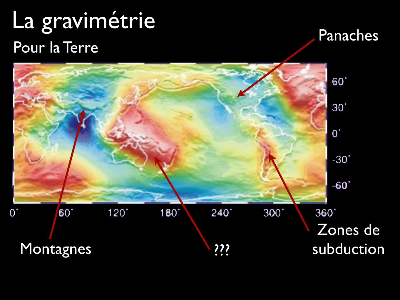
Panaches

Zones de subductionMontagnes ???

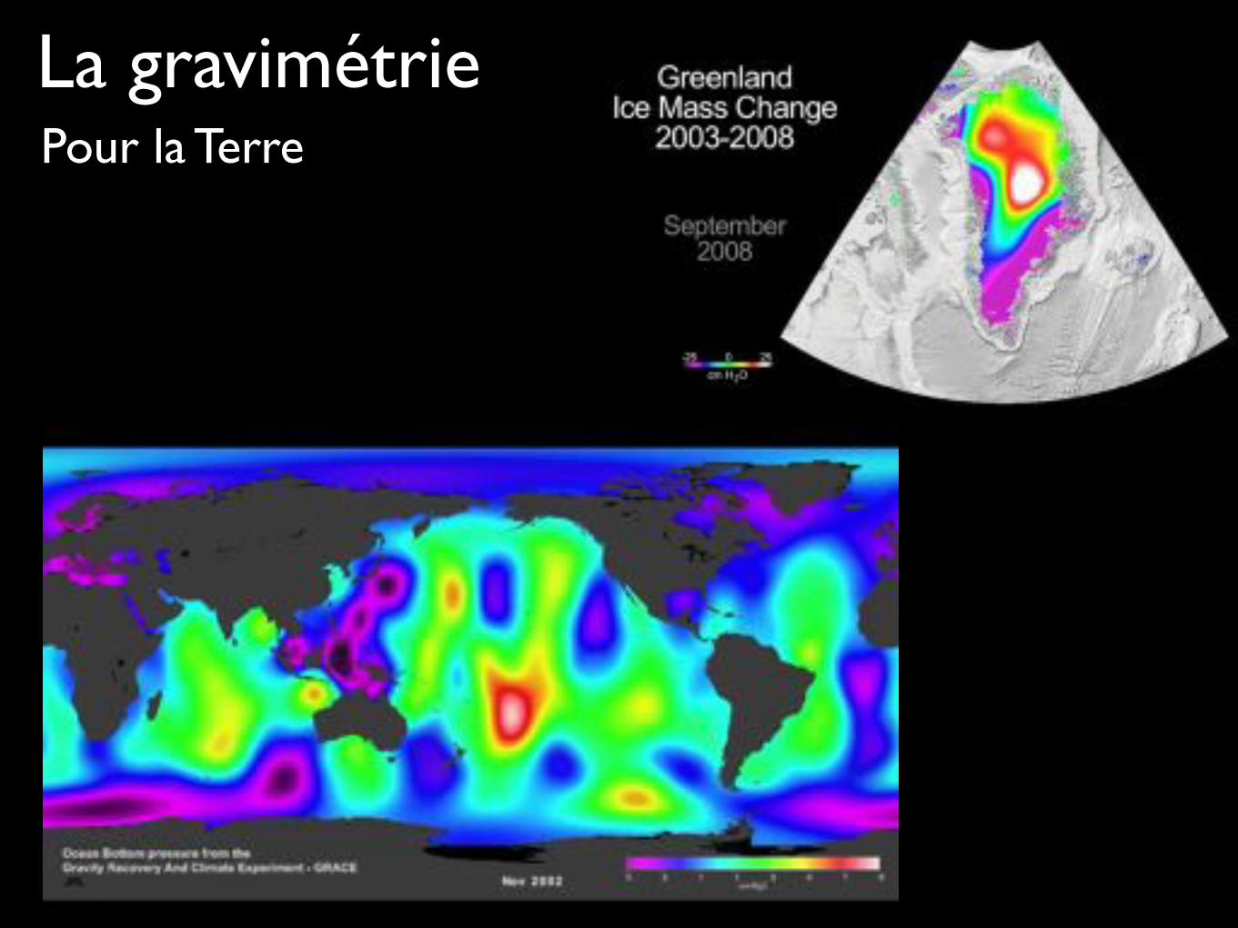
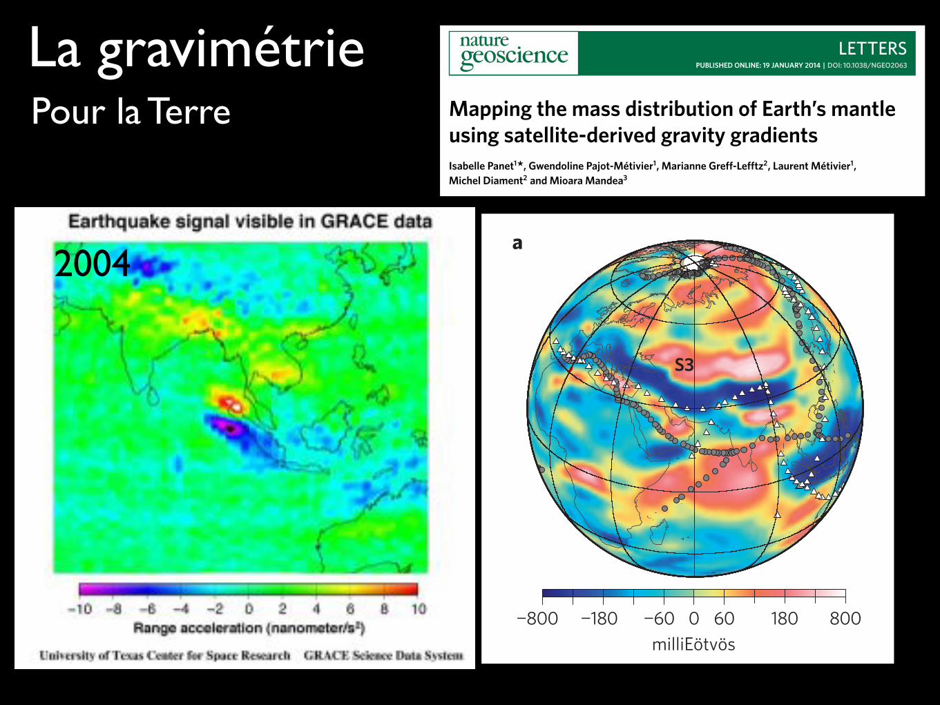
La gravimétriePour la Terre


LETTERS

NATURE GEOSCIENCE DOI: 10.1038/NGEO2063

dVs/Vs (%)

0 60¬60 180¬180 800¬800milliEötvös

0.0 0.3¬0.3 0.6¬0.6 0.9¬0.9 1.2¬1.2

S3

a b

Figure 4 | XX gravitational gradients and S40RTS and DR2012 shear-velocity anomalies. a, Second-order derivatives in the X/north direction centred onAsia (left), of the Earth’s non-hydrostatic gravitational potential along the GOCE orbit, smoothed at 5� resolution. Past subduction zones geometries16 aredrawn as in Fig. 1. b, Contours of the shear-velocity anomalies dVs/Vs from the S40RTS model22 between 1,300 and 1,400 km are shown (middle), as wellas those from the DR2012 upper mantle model28 at 550 km depth (right). They illustrate the east–west directionalities in the tomographic models between1,000 and 1,500 km, and around 550 km, along the former Tethys margin.

widens (which happens when slabs flatten at the upper–lowermantle boundary or merge in the lower mantle, or for largesuperplumes), our tests show that deeper layers can be reached,down to at least some 2,500 kmdepth for a 4,000-kmwide anomaly.Besides, in contrast to geoid data, the gradients bring an enhancedgeometric characterization of the mass distribution, resulting fromtheir very nature of directional differences, thus facilitating com-parisons with seismic tomography. This is illustrated in Fig. 2,revealing that, besides changing sign between the upper and thelower mantle, the gradients delineate more and more closely theslab borders as depth decreases. For a 4,000-kmwidemass anomaly,significant oscillations at the edges of the mass distribution ap-pear in the signal when the anomaly is shallower than 1,700 km(see Supplementary Information). This is the reason why, for theinvestigated class of signals, smooth gradient variations probablyindicate deep sources.

From the above analysis, confirmed by a comparison with thefast seismic velocity anomalies of the S40RTS model22, we canidentify the mantle structures evidenced in our maps. We interpretthe three-lobe anomaly in the YY gradients over North andCentral America (Fig. 3a, anomaly S1) as tracking the subductedFarallon lithosphere in the upper lower mantle. Consistently, a fastnorth–south seismic velocity anomaly is found between 900 and1,600 km (refs 8,22,23), coinciding with the central negative lobeof the YY anomaly (see Fig. 3b). Over Asia, the broader positiveYY pattern (Fig. 3a, anomaly C1) is probably related to deeperand wider mass anomalies, and we find consistent fast seismicvelocities between 1,700 and 2,600 km depth (see Fig. 3b). This canreflect mid-mantle remnants of subducted Jurassic lithosphere22,24.In these areas, the lower mantle mass signal overprints notonly the lithosphere signal, reduced by isostasy at the gradientscales, but also the upper mantle signal. This arises from thecorrespondence between the differentiation directions and thenorth–south/east–west global structure of the deep Earth, involvinglarge amounts of mass. Formed as a result of the stability of nearlynorth–south subductions around the Pacific region over the past250Myr (ref. 25), the wide downwelling ring of slabs partitioningthe lower mantle is strongly directional and, therefore, naturallyhighlighted by the satellite gradients. Thus, around the Japanesearc, where slabs are thought to stagnate at the transition zone(ref. 26), thereby reducing the upper lower mantle directionalheterogeneity, the gradient signal is low (Fig. 3a, anomaly S2).We finally note that the observed YY gradients are smoother

than those from the mantle model, where the slab density andgeometry do not change with depth. These discrepancies indicatelimits of the model, which does not include the processes ofslab accumulation in the lower mantle, suggested below Asia, norslab stagnation around the transition zone, suggested below theJapanese subduction.

A more complex XX gradients pattern is observed along theformer Tethyan margin (Fig. 4a, anomaly S3), with two differentscales. The directions coincide with those of a fast velocity anomalybetween 1,000 and 1,500 km depth18,27, which may explain thelarge-scale positive lobe of the gradient anomaly in the IndianOcean. Furthermore, the strength of a smaller scale componentmay point to an important east–west structuring in the uppermantle along the former subduction boundary, also suggested by anelongated east–west velocity anomaly at 550 km depth in an uppermantle tomographic model28 (Fig. 4b), resolved at 500 km depthin the model of ref. 29. Because gradient anomalies change signwith the source depth, the observed composite pattern may helpdifferentiate between upper and lower mantle structures, such asthe subducted Indian plate and the earlier subducted Tethys slabs,shedding light on howplatemovements relate tomantle flows.

If the GOCE mission originally targeted the Earth’s shallowlayers, our gravitational gradient maps offer a new scope to gra-diometry from space: mantle dynamics. The geometric consis-tency of gravity gradients and seismic velocities indicates thatthey can be combined to decipher the mantle density and vis-cosity structure30 from global to regional scales, less emphasizedin the smooth geoid, and help identify the physical mechanismsreflected by seismic velocity variations. From this combination,new insights are expected on the mantle temperature and com-position variations associated with density and seismic veloci-ties anomalies. Inconsistencies between the datasets might alsopoint to mechanisms not associated with density variations, suchas anisotropy and stress. Probing the path and chemical evo-lution of the subducted tectonic plates, and the induced vis-cous flows, the gradients should give new clues towards under-standing the mantle vertical mixing. This picture on slab de-scent and accumulation may also help illuminate the deepestmantle structure and geodynamics. This new field of applica-tions of gravity gradients calls for a joint analysis with othergeophysical data, flow models and tectonic plate history recon-structions, opening new avenues to integrated global dynamicmodels of the Earth.

4 NATURE GEOSCIENCE | ADVANCE ONLINE PUBLICATION | www.nature.com/naturegeoscience

LETTERS

PUBLISHED ONLINE: 19 JANUARY 2014 | DOI: 10.1038/NGEO2063

Mapping the mass distribution of Earth’s mantleusing satellite-derived gravity gradientsIsabelle Panet1*, Gwendoline Pajot-Métivier1, Marianne Greff-Lefftz2, Laurent Métivier1,Michel Diament2 and Mioara Mandea3

The dynamics of Earth’s mantle are not well known1.Deciphering mantle flow patterns requires an understand-ing of the global distribution of mantle density2,3. Seismictomography has been used to derive mantle density dis-tributions, but converting seismic velocities into densitiesis not straightforward4,5. Here we show that data fromthe GOCE (Gravity field and steady-state Ocean CirculationExplorer) mission6 can be used to probe our planet’s deepmass structure. We construct global anomaly maps of theEarth’s gravitational gradients at satellite altitude and use asensitivity analysis to show that these gravitational gradientsimage the geometry of mantle mass down to mid-mantledepths. Our maps highlight north–south-elongated gravitygradient anomalies over Asia and America that follow a beltof ancient subduction boundaries, as well as gravity gradientanomalies over the central Pacific Ocean and south of Africathat coincide with the locations of deep mantle plumes. Weinterpret these anomalies as sinking tectonic plates andconvective instabilities between 1,000 and 2,500 km depth,consistent with seismic tomography results. Along the formerTethyan Margin, our data also identify an east–west-orientedmass anomaly likely in the upper mantle. We suggest that bycombining gravity gradientswith seismic and geodynamic data,an integrated dynamicmodel for Earth can be achieved.

Understanding our planet’s evolution requires elucidation ofits internal structure and composition, as well as the mechanismof its heat loss. Over the past decades, tremendous advanceshave been gained from seismological, geochemical and geologicaldata interpretation, mineral physics experiments and numericalmodelling. Yet, unravelling the deep Earth’s dynamics and itsinterplay with surface tectonics is still hampered by the lackof information on the global density distribution, responsiblefor the buoyancy forces driving the mantle flows and the platemotions, and on the viscosity, which controls the convectiveflows1–3. The seismic tomography provides an image of theglobal three-dimensional internal structure through maps of fastand slow seismic anomalies, which delineate deep convectiveinstabilities and, at relatively smaller scales, plates sinking into themantle7,8. However, converting seismic velocities into densities isnot straightforward, as both depend on temperature and chemicalcomposition and are strongly affected by phase changes—thesethree factors influencing each other4. Also, seismic velocities cangreatly vary with direction through non-density contrast-inducedmechanisms, such as anisotropic crystal alignment by flow ornon-hydrostatic stresses5. Hence, we need further information tointerpret the seismic signal in terms of density variations versus

1Institut National de l’Information Géographique et Forestière, Laboratoire LAREG, Université Paris Diderot, GRGS, Bat. Lamarck A, Case 7071, 35 rueHélène Brion, 75205 Paris Cedex 13, France, 2Université Paris Diderot, Sorbonne Paris-Cité, Institut de Physique du Globe de Paris, UMR 7154 CNRS,F-75013 Paris, France, 3Centre National d’Etudes Spatiales, 2, place Maurice Quentin, 75039 Paris, France. *e-mail: [email protected]

other physical processes. Global data to describe the densitydistribution at depth are thus essential to get a full picture of ourplanet’s dynamics2,9,10.

With the European Space Agency’s Gravity field and steady-stateOcean Circulation Explorer (GOCE) satellite6, a new class ofobservations has emerged to probe the Earth’s interior structure:satellite gravity gradients. Originally imagined by Cavendish in thelate 18th century to accurately determine the Earth’s density fromthe gravity differences between close points, this early measure-ment concept experienced a recent growth to image the Earth’ssubsurface. Because they sense tiny variations of the gravity vectorin different directions, gravity gradients are much more sensitiveto the spatial structure and directional properties of the attract-ing masses than classical observations on gravitational intensity11.Tracking distance changes due to gravitational attraction differ-ences between two co-orbiting satellites12, the GRACE missionopened the way towards realizing this concept by satellites, afterthe first gravity observations from space made by CHAMP. Thefull gravitational gradient tensor has been measured from spacefor the first time by the GOCE mission. With its three pairs ofultra-sensitive accelerometers perceiving gravitational accelerationslightly differently onboard the satellite, the GOCE space gradiome-ter indeed measures, on a 255-km altitude orbit, the second-orderderivatives of the gravitational potential in all directions13 (seeSupplementary Information).

Reaching their optimal accuracy at scales smaller than 750 km,the gradiometric measurements are combined with a GOCE-orbitbased model, dominating at scales larger than ⇠1,000–1,200 km.From these data along the orbit, expressed in a north–west-upframe by the GOCE High-level Processing Facility14, we builtglobal anomaly maps of the Earth’s gravitational gradients atsatellite altitude with respect to an Earth model obtained fromthe hydrostatic equilibrium of a rotating preliminary referenceEarth model (PREM)-layered15 spheroid (see SupplementaryInformation). The obtained anomalies reflect irregularities inthe mass distribution and interface deflections with respect tothe reference model (Fig. 1a). Because they are calculated atthe GOCE altitude, we avoid noise amplification resulting fromthe downward continuation to the Earth’s surface. Their longwavelength components—which could also be studied fromGRACE data—rely on directional information from the gradientsrather than gradiometer accuracy. Whereas the radial gradient isisotropic, the north and west derivatives emphasize mass anomaliesorthogonal to the differentiation direction. Local mass anomaliesrelated to mountain chains and subduction, oceanic ridges andplateaux leave elongated patterns at small scales. Furthermore,

NATURE GEOSCIENCE | ADVANCE ONLINE PUBLICATION | www.nature.com/naturegeoscience 1

2004

La gravimétrieAvantages : facile, pas trop cher, problème linéaire, informations structurales et dynamiques

Inconvénient : données “intégratives”, résolution détaillée pas possible partout, problème non-unique

La sismologieAvantages : de + en + facile, information en volume

Inconvénient : dépend de la distribution des séismes, information structurale.

La sismologieRadiographie de la Terre par rayons...sismiques

17 Avril 1889Premier enregistrement d’un séisme lointain à Potsdam par E. von Rebeur-Pacshwitz (Nature, 1889).Le séisme a eu lieu au Japon (magnitude ~5.8)

Les ondes sismiques se propagent dans la Terre et

permettent son auscultation!

1972 : Tomographie médicale, rayons X

La Terre sismologique... après1960

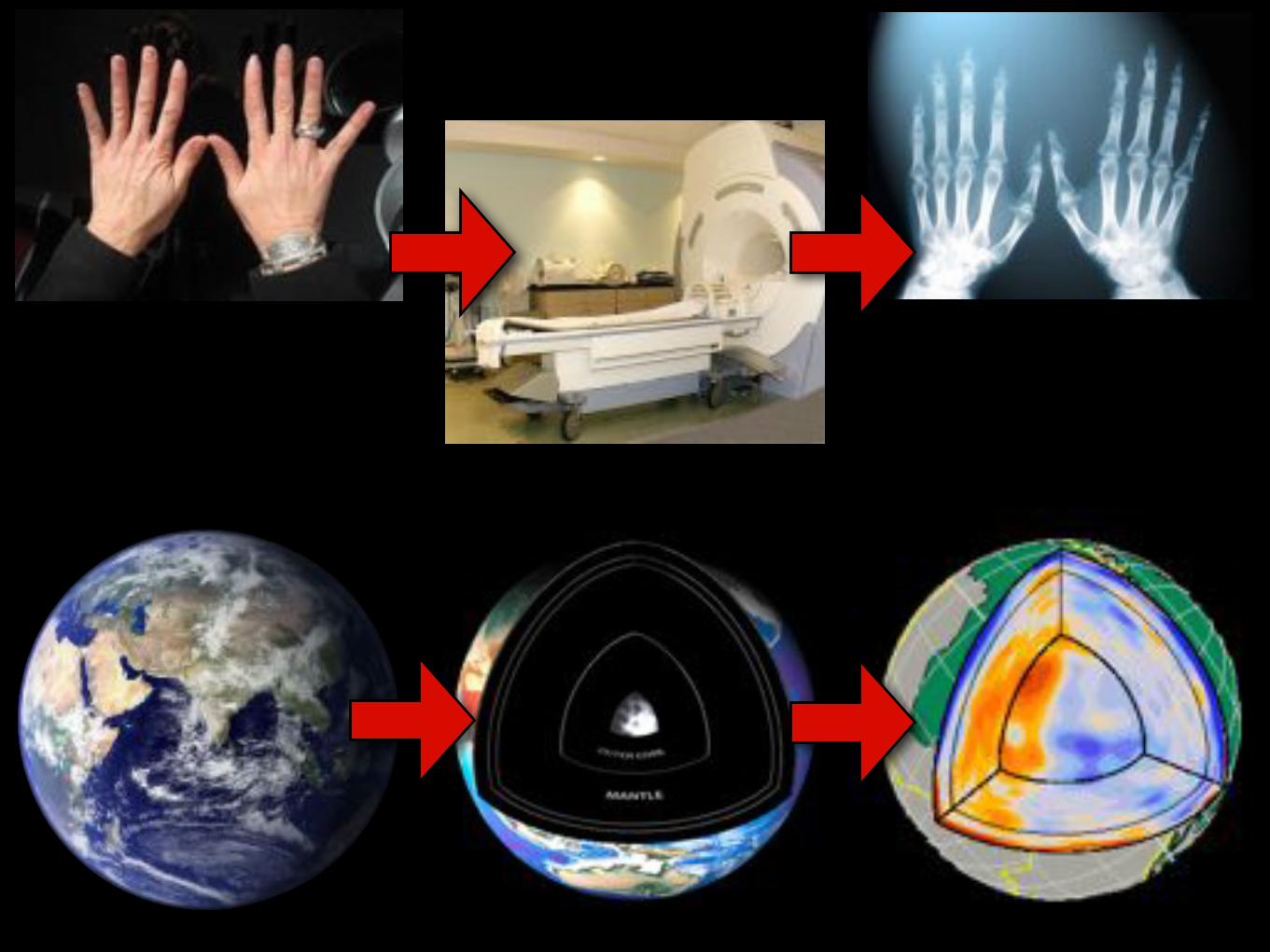
Quelle(s) source(s) pour ausculter la Terre?

La sismologieQu’est-ce qu’on voit ?

Hodochrones

Modèle de Terre (vitesse, densité) pour expliquer au mieux les données

Densité Ondessismiques

La sismologieQu’est-ce qu’on voit ?

Sa structure radialeDes hétérogénéités

latérales

La Terre sismologique...Les premiers modèles...

Dziewonsky, 1984

La Terre sismologique...Les modèles actuels...

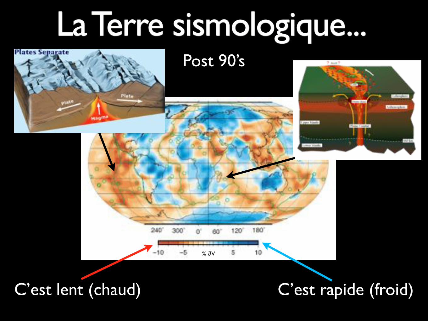
% ∂V

C’est lent (chaud) C’est rapide (froid)

La Terre sismologique...Post 90’s

Grand et al., 1997

Les zones de subduction

Wortel & Spakman, 2000

La sismologiePour la lune

Apollo (11-)12-14-15-164 sismomètres (1969-1977)séismes lunaires:moonquakes

Buzz Aldrin installant le sismomètre d’Apollo 11


THE CRUSTTwo key parameters used in deciphering both lunar evolu-tion and the lunar samples are the average thickness of the crust and how the crustal thickness varies from place to place. As an example, the average crustal thickness is believed to be a direct by-product of the Moon’s initial differentiation; it therefore depends upon several factors, including the depth of the magma ocean and the efficiency with which crystallizing plagioclase was able to float (e.g. Solomatov 2000). Data obtained from seismometers placed on the lunar surface at the Apollo 12, 14, 15, and 16 stations offer the most direct means of assessing this quantity (see FIGURE 1 for the locations of the Apollo and Luna sampling stations and the outline of the Apollo seismic network). Analyses during the Apollo era suggested initially that the crust beneath the “Apollo zone” was about 60 km thick. However, recent independent analyses by two different research groups now suggest that the crustal thickness is much less in this area, probably somewhere between about 30 and 38 km (Khan and Mosegaard 2002; Lognonné et al. 2003). While one might think that this dramatic revi-sion would have large consequences on estimates of the bulk composition of the Moon, it is now realized that the globally averaged thickness of the crust is somewhat greater than that measured beneath the Apollo stations (the glob-ally averaged thickness is probably between 40 and 45 km; see Chenet et al. 2006 and Hikida and Wieczorek 2007). Nevertheless, as a complicating factor, several measure-ments show that there are also large lateral and vertical variations in the composition of the crust, which were not fully appreciated until after the Clementine and Lunar Prospector missions (Jolliff et al. 2000). In particular, orbital gamma-ray data and in situ heat-flow measurements indicate that heat-producing and incompatible elements are concentrated within a single geologic province that

encompasses Mare Imbrium and Oceanus Procellarum (i.e. the Procellarum KREEP Terrane; see Wieczorek and Phillip 2000), and remote sensing data show that the surrounding highlands crust becomes increasingly mafic with depth.

One of the problems with the Apollo seismic data is that the network spans only a small portion of the Moon’s central nearside hemisphere. Fortunately, the thickness of the crust can be estimated outside of the Apollo zone by using a combination of the Moon’s surface relief, gravita-tional field, and reasonable assumptions about the density of the crust and mantle. FIGURE 2 shows the topography of the Moon (upper left) obtained by the Clementine mission (Smith et al. 1997; USGS 2002), as well as the best estimate of the radial gravitational acceleration at the surface (upper right), derived primarily from the Lunar Prospector mission (Konopliv et al. 2001). Since the gravitational field is obtained by measuring small Doppler shifts in radio signals emitted by orbiting spacecraft, the resolution over the farside hemisphere of the Moon, where spacecraft are not visible from Earth, is considerably poorer than for the near-side hemisphere. Immediately visible in the topographic image are the depressions associated with numerous giant impact basins—the giant basin on the farside hemisphere is the South Pole–Aitken basin, which is currently the largest recognizable impact structure in the solar system. Furthermore, some of the impact basins are seen to possess large central positive gravitational anomalies, which are colloquially referred to as “mascons,” short for mass concentrations. While the origin of mascons is not completely resolved, it is likely that they result from a combination of dense mare basaltic lava flows (which are perhaps several kilometers thick in places) and structural uplift of relatively dense mantle materials (for a review, see Wieczorek et al. 2006).

FIGURE 1 Apollo landing sites (stars) and Luna sam-ple-return stations (circles). The Apollo seismic network comprises four stations, forming a triangle with distances between vertices of about 1200 km. BASEMAP FROM HIESINGER AND HEAD 2006


Apollo (11-)12-14-15-164 sismomètres (1969-1977)séismes lunaires:moonquakes

Wieckzoreck, 2009


above observations is that numerous magma-filled fractures currently located in the deep mantle are capable of relieving the small stresses induced by Earth-raised tides.

Analyses of the Apollo seismic data have given rise to a data set of P- and S-wave first-arrival times from which it is possible to invert for a seismic velocity profile of the crust and mantle. Several investigations have attempted to do this, and a debate has arisen as to whether or not any seismic discontinuities exist in the lunar mantle. The final Apollo-era analysis indicated that a discontinuity might potentially exist about 500 km below the surface, and many researchers subsequently assumed that this depth most plausibly represented the base of the lunar magma ocean. A reanalysis of these data by one group confirmed that a discontinuity at this depth was probable (Khan and Mosegaard 2002); however, an independent analysis by a second group, using a somewhat different data set, obtained a contradictory result (Lognonné et al. 2003). A more recent inversion by the first group using a different meth-odology showed that they could in fact fit the seismic data using a mantle that was homogeneous in elemental compo-sition and that did not possess any discontinuities at all (Khan et al. 2007).

Given that seismology is one of the most powerful tech-niques for investigating the interior structure and composi-tion of a planetary body, it is somewhat disappointing that no consensus has arisen in regard to the lunar mantle. The range of possibilities presented by these studies is in some sense related to the data themselves. In particular, given the weak nature of the deep moonquakes, the uncertainty in the first-arrival times can sometimes exceed 10 seconds. Furthermore, there are currently two independent arrival-time data sets, and each of these has been subjected to a different set of analysis techniques. Regardless of the quality of the existing data, one needs to keep in mind that the Apollo seismic network only covered a very limited portion of the Moon’s surface and that its eight years of operation represent only a fraction of the largest tidal peri-odicity of 18.6 years. Given that mare volcanism occurred primarily on the nearside hemisphere of the Moon, it is

quite possible that the seismic properties of the farside hemisphere will turn out to be much different from those beneath the Apollo network.

The origin of the deep moonquakes, as well as the nature by which energy is dissipated in the deep mantle, could be further addressed if the temperature profile of the Moon was known. Two techniques used to constrain this have exploited the known dependence of a mineral’s seismic velocity and electrical conductivity on temperature. The electrical-conductivity profile of the Moon has been esti-mated by using electromagnetic-sounding techniques, whereby the relationship between simultaneous time varia-tions in the ambient magnetic field as measured from orbit and the resulting field measured on the surface was analyzed (for a review, see Hood 1986). By calculating hypothetical mineral assemblages that would be stable at a given temperature, it was possible to invert for not only the mantle temperature profile, but also its composition. Unfortunately, the current electromagnetic and seismic data sets only place weak constraints on the interior temperature profile. Nonetheless, these analyses indicate that the lunar mantle is composed primarily of olivine and orthopyroxene, with lesser abundances of clinopyroxene and garnet (Khan et al. 2006, 2007).

THE COREAll of the terrestrial planets and many of the icy satellites in the outer solar system possess iron-rich cores whose size is about half the radius of the parent body (the core of Mercury is probably somewhat larger). While the Moon too probably possesses some kind of core, its relative size is thought to be considerably smaller. In particular, anal-yses of the Moon’s mass, radius, and moment of inertia (a measure that is sensitive to how density varies with depth) imply that if the Moon does possess an iron-rich core, it must be smaller than about 460 km, which is only about one-quarter of the Moon’s radius (for reviews, see Hood 1986 and Wieczorek et al. 2006). Other geophysical obser-vations are generally consistent with this picture. Namely, electromagnetic-sounding data place an upper limit of about 500 km on the core radius (Hood 1986), and the

FIGURE 3 P-wave (upper) and S-wave (lower) ray paths in the Moon

as viewed from each seismic station as a function of epicentral distance and hypocenter depth (after Lognonné et al. 2003). Deep moon quakes are in blue, shallow moonquakes are in green, and the artificial and meteoroid impacts are in red. The light concentric circles correspond to artificial seismic discontinuities that were used in creating the seismic velocity model.


measurement of a weak, induced dipolar magnetic field as the Moon passes through the Earth’s geomagnetic tail implies the existence of a high-electrical-conductivity core with a radius of about 360 km (Hood et al. 1999). Furthermore, analyses of minute rotational signatures obtained from the lunar laser ranging experiment indicate that energy is currently being dissipated at the boundary between a molten core and solid mantle of approximately the same radius (Williams et al. 2001).

If the Moon does indeed possess an iron-rich core, then it is possible that it could have generated a dipolar magnetic field at some point in its history. Some of the lunar samples have strong magnetizations (see Fuller and Cisowski 1987), and orbital magnetic measurements from the Lunar Prospector mission show that portions of the crust are magnetized (see FIG. 2, lower right, for one model of the magnetic-field strength; Purucker 2008). Some of these magnetizations could potentially have been acquired as magmatic rocks cooled in the presence of a stable, internal dipolar field. If true, the limited magnetization age constraints from the lunar samples appear to suggest that such a dynamo might have turned on relatively late (~3.9 billion years ago) and lasted for only a short duration (see Stegman et al. 2003). A potential problem with the dynamo hypothesis, however, is that the implied field strengths are difficult to generate from a core as small as the Moon’s. As an alternative hypothesis, large impact events could have generated strong transient fields that magnetized portions of the lunar crust. In support of this scenario, high crustal fields appear to be correlated with basin ejecta deposits (Halekas et al. 2001). Furthermore, a curious correlation exists between some strong crustal fields and the antipodes of some of the youngest and largest impact basins, such as Imbrium, Serenitatis, Orientale, and Crisium. One explana-tion for this observation is that these impact events might have generated a partially ionized plasma cloud that expanded around the Moon and amplified ambient fields (of either internal or external origin) at the point diametri-cally opposite the crater (Hood and Artemieva 2008). A currently unresolved issue of great importance is whether the magnetic fields as observed from orbit are a conse-quence of magnetized sources that are located at the surface (such as impact ejecta) or deep in the crust (such as from magmatic intrusions).

While the available evidence indicates that the Moon possesses a small molten core, the geophysical data cannot unambiguously constrain its composition. Nearly pure molten iron or molten iron-sulfide compositions are both compatible with the available constraints. Indeed, one could even explain the available data with a core composed of a dense silicate magma that was rich in iron and tita-nium (Wieczorek et al. 2006). Perhaps the best way to discriminate among these possibilities would be to deter-mine the seismic velocity of the core. Unfortunately, as is evident from FIGURE 3, none of the well-determined ray paths pass through the deepest portion of the lunar interior.

SYNTHESISFIGURE 4 shows one interpretation of the Moon’s interior structure based on geophysical measurements. Seismic, gravity, and topography data suggest that the crust is on average about 40–45 km thick and that it is considerably thinned beneath the largest impact basins. Furthermore, seismic data show that a few energetic moonquakes occur per year within the crust and upper mantle, and a probable explanation for these events is that they are caused by the slow accumulation of stresses as the Moon cools and contracts over time. The seismic data are at present some-

what ambiguous as to whether or not there are any seismic discontinuities in the mantle, though some studies are consistent with one being present about 500 km below the surface. Even if this discontinuity exists, the limited spatial distribution of the detected seismic events does not allow one to say if this is a global feature or if it is present only beneath the Apollo network, which was emplaced on the volcanically active nearside of the Moon. Deep in the Moon, about 1000 km below the surface, about 300 moon-quake “nests” are repeatedly activated by the tides raised by Earth. While the locations of these nests are almost all found on the nearside hemisphere, perhaps consistent with an aseismic farside, the seismic and lunar laser ranging data indicate that the deepest portion of the mantle is highly attenuating and might perhaps be partially molten. If the deepest mantle were sufficiently attenuating, the nearside Apollo network might not be able to detect deep farside moonquakes. Several lines of evidence are consistent with the Moon possessing a dense molten core (<460 km radius), but its composition is not well constrained by the available data. Nevertheless, regardless of the core’s compo-sition, thermal-evolution models suggest that its tempera-ture is probably low enough to have allowed some portion of it to crystallize, forming an even smaller solid inner core.

FUTURE MISSIONSThe fact that a schematic diagram of the lunar interior can be drawn at all is a testament to the geophysical data that have been collected both from orbit and from the network of surface stations emplaced during the Apollo missions. Nevertheless, many unresolved questions about the interior of the Moon remain, particularly in regard to the composi-tion of the mantle and core. Fortunately, geophysical measurements will be obtained from several spacecraft that are currently in orbit at the time of this writing or will be placed into orbit over the next several years. As examples, the Japanese Kaguya, Chinese Chang’e-1, and Indian Chandrayaan-1 missions are currently making precise topographic maps of the Moon, and this map will be further improved with the launch of the American Lunar Reconnaissance Orbiter in 2009. (Prior to these missions, the topography of both Venus and Mars was known more precisely than that of the Moon.) The Kaguya mission contains an orbital radar sounder that will attempt to deter-mine the thickness of the mare basalts, map the thickness of the regolith, and detect buried regolith horizons. Kaguya

FIGURE 4 Schematic diagram of the Moon’s interior structure as determined by geophysical means. Apollo landing sites

are indicated by squares. FROM WIECZOREK ET AL. 2006


deepmoonquake

shallowmoonquake

impacts

deep ~2000/animpacts ~200/anshallow ~5/an

Wieckzoreck, 2009

La sismologie + la gravimétriePour la lune

La sismologiePour Mars

- 1975 : Vicking pose 2 sismomètres

- 2016 : InSight posera 1 sismomètre

InSight Nasa mission

• Structure interne?

• Source du volcanisme?

• Source du faible champ magnétique?

La sismologiePour Mars

Les sources pour imag(in)er ?

suggest that such a statistical treatment canbe applied to nonthermal random wave-fields, in particular to long series of ambientseismic noise, because the distribution of theambient sources randomizes when averagedover long times. Ambient seismic noise isadditionally randomized by scattering fromheterogeneities within Earth (18). Surfacewaves are most easily extracted from theambient noise (5), because they dominate theGreen function between receivers located atthe surface and also because ambient seismicnoise is excited preferentially by superficialsources, such as oceanic microseisms andatmospheric disturbances (19–22). The seis-mic noise field is often not perfectly isotropicand may be dominated by waves arrivingfrom a few principal directions. To reduce thecontribution of the most energetic arrivals, wedisregard the amplitude by correlating onlyone-bit signals (15, 17) before the computa-tion of the cross-correlation.

Examples of cross-correlations betweenpairs of seismic stations in California appearin Fig. 1 (23). Cross-correlations betweentwo station pairs (MLAC-PHL and SVD-MLAC) in two short-period bands (5 to 10 sand 10 to 20 s) are presented using fourdifferent 1-month time series (January,April, July, and October 2002). For eachstation pair, results from different months aresimilar to one another and to the resultsproduced by analyzing a whole year of data,but differ between the station pairs. Thus, theemerging waveforms are stable over timeand characterize the structure of the earthbetween the stations. In addition, the cross-correlations of noise sequences are verysimilar to surface waves emitted by earth-quakes near one receiver observed at theother receiver. This confirms that the cross-correlations approximate Green functions ofRayleigh waves propagating between eachpair of stations and that 1 month of datasuffices to extract Rayleigh-wave Greenfunctions robustly in the period band ofinterest here (7 to 20 s).

We selected 30 relatively quiescent days(during which no earthquakes stronger thanmagnitude 5.8 occurred) of continuous datataken at a rate of one sample per secondfrom 62 USArray stations within California(24) during August and September 2004.Short-period surface-wave dispersion curvesare estimated from the Green functions usingfrequency-time analysis (25–27) from the1891 paths connecting these stations. Werejected waveforms with signal-to-noise ra-tios smaller than 4 and for paths shorter thantwo wavelengths, resulting in 678 and 891group-speed measurements at periods of 7.5and 15 s, respectively (fig. S2). We thenapplied a tomographic inversion (28) to thesetwo data sets to obtain group-speed maps ona 28 ! 28 km grid across California (Fig. 2).

10 - 20 s 10 - 20 s

5 - 10 s5 - 10 s

B D

C Eevent 2 - MLAC

SVD - MLAC

SVD - MLAC

23510

2351023510

23510

event 1 - PHL

MLAC - PHL

MLAC - PHL

event 1 - PHL

MLAC - PHL

MLAC - PHL

event 2 - MLAC

SVD - MLAC

SVD - MLAC

-120 -115

35

38

1

2

3 4

6

5

GreatGreatBasinBasinGreatBasin

Transverse RangesTransverse RangesTransverse Ranges

Peninsular

Peninsular

Ranges

Ranges

Peninsular

Ranges

Imperial

Imperial

ValleyValley

Imperial

Valley

Diablo R

ange

Diablo R

ange

Sacram

ento

Sacram

ento

Basin

Basin

Diablo R

ange

Sacram

ento

Basin

PHL

MLAC

SVD

1

2

Co

a s t Ra n

ge s

Co

a s t Ra n

ge s

Co

a s t Ra n

ge s

Si e

r r a N

ev

ad

a

Si e

r r a N

ev

ad

a

Si e

r r a N

ev

ad

a

Sa n

J oa q

ui n

Sa n

J oa q

ui n

Ba s i n

Ba s i n

Sa n

J oa q

ui n

Ba s i n

Ce

nt r a

l Va

l l ey

Ce

nt r a

l Va

l l ey

Ce

nt r a

l Va

l l ey

M o j a v e D e s e r tM o j a v e D e s e r tM o j a v e D e s e r t

A

Group velocity (km/s)

Group velocity (km/s) Group velocity (km/s)


Fig. 1. Waveforms emerging from cross-correlations of ambient seismic noise compared withRayleigh waves excited by earthquakes. (A) Reference map showing the locations of the principalgeographical and geological features discussed in the text. White triangles show the locations ofthe USArray stations used in this study (5 of the 62 stations are located north of 40-N). Blue andred solid lines are the locations of known active faults. Yellow rectangles with digits indicate thefollowing features: (1) Los Angeles Basin, (2) Ventura Basin, (3) San Andreas Fault, (4) GarlockFault, (5) Mojave shear zone, and (6) Stockton Arch. (B) Comparison of waves propagatingbetween stations MLAC and PHL [yellow triangles in (A)], bandpassed over periods between 5 and10 s. The upper trace (black) is the signal emitted by earthquake 1 [white circle with red number in(A)] near MLAC observed at PHL; the middle trace (gold) is the cross-correlation from 1 year ofambient seismic noise observed at stations MLAC and PHL; and the lower traces are cross-correlations from 4 separate months of noise observed at the two stations in 2002 (magenta,January; red, April; green, July; blue, October). The earthquake-emitted signal was normalized tothe spectrum of the cross-correlated ambient noise. (C) Similar to (B), but with the bandpass filterat periods between 10 and 20 s. (D) Similar to (B), but between stations SVD and MLAC [yellowtriangles in (A)]. Earthquake 2 is near station SVD, observed at station MLAC. (E) Similar to (D), butwith the bandpass filter at periods between 10 and 20 s.

R E P O R T S

11 MARCH 2005 VOL 307 SCIENCE www.sciencemag.org1616

on

Sept

embe

r 29,

200

9 w

ww

.sci

ence

mag

.org

Dow

nloa

ded

from

suggest that such a statistical treatment canbe applied to nonthermal random wave-fields, in particular to long series of ambientseismic noise, because the distribution of theambient sources randomizes when averagedover long times. Ambient seismic noise isadditionally randomized by scattering fromheterogeneities within Earth (18). Surfacewaves are most easily extracted from theambient noise (5), because they dominate theGreen function between receivers located atthe surface and also because ambient seismicnoise is excited preferentially by superficialsources, such as oceanic microseisms andatmospheric disturbances (19–22). The seis-mic noise field is often not perfectly isotropicand may be dominated by waves arrivingfrom a few principal directions. To reduce thecontribution of the most energetic arrivals, wedisregard the amplitude by correlating onlyone-bit signals (15, 17) before the computa-tion of the cross-correlation.

Examples of cross-correlations betweenpairs of seismic stations in California appearin Fig. 1 (23). Cross-correlations betweentwo station pairs (MLAC-PHL and SVD-MLAC) in two short-period bands (5 to 10 sand 10 to 20 s) are presented using fourdifferent 1-month time series (January,April, July, and October 2002). For eachstation pair, results from different months aresimilar to one another and to the resultsproduced by analyzing a whole year of data,but differ between the station pairs. Thus, theemerging waveforms are stable over timeand characterize the structure of the earthbetween the stations. In addition, the cross-correlations of noise sequences are verysimilar to surface waves emitted by earth-quakes near one receiver observed at theother receiver. This confirms that the cross-correlations approximate Green functions ofRayleigh waves propagating between eachpair of stations and that 1 month of datasuffices to extract Rayleigh-wave Greenfunctions robustly in the period band ofinterest here (7 to 20 s).

We selected 30 relatively quiescent days(during which no earthquakes stronger thanmagnitude 5.8 occurred) of continuous datataken at a rate of one sample per secondfrom 62 USArray stations within California(24) during August and September 2004.Short-period surface-wave dispersion curvesare estimated from the Green functions usingfrequency-time analysis (25–27) from the1891 paths connecting these stations. Werejected waveforms with signal-to-noise ra-tios smaller than 4 and for paths shorter thantwo wavelengths, resulting in 678 and 891group-speed measurements at periods of 7.5and 15 s, respectively (fig. S2). We thenapplied a tomographic inversion (28) to thesetwo data sets to obtain group-speed maps ona 28 ! 28 km grid across California (Fig. 2).

10 - 20 s 10 - 20 s

5 - 10 s5 - 10 s

B D

C Eevent 2 - MLAC

SVD - MLAC

SVD - MLAC

23510

2351023510

23510

event 1 - PHL

MLAC - PHL

MLAC - PHL

event 1 - PHL

MLAC - PHL

MLAC - PHL

event 2 - MLAC

SVD - MLAC

SVD - MLAC

-120 -115

35

38

1

2

3 4

6

5

GreatGreatBasinBasinGreatBasin

Transverse RangesTransverse RangesTransverse Ranges

Peninsular

Peninsular

Ranges

Ranges

Peninsular

Ranges

Imperial

Imperial

ValleyValley

Imperial

Valley

Diablo R

ange

Diablo R

ange

Sacram

ento

Sacram

ento

Basin

Basin

Diablo R

ange

Sacram

ento

Basin

PHL

MLAC

SVD

1

2

Co

a s t Ra n

ge s

Co

a s t Ra n

ge s

Co

a s t Ra n

ge s

Si e

r r a N

ev

ad

a

Si e

r r a N

ev

ad

a

Si e

r r a N

ev

ad

a

Sa n

J oa q

ui n

Sa n

J oa q

ui n

Ba s i n

Ba s i n

Sa n

J oa q

ui n

Ba s i n

Ce

nt r a

l Va

l l ey

Ce

nt r a

l Va

l l ey

Ce

nt r a

l Va

l l ey

M o j a v e D e s e r tM o j a v e D e s e r tM o j a v e D e s e r t

A


Group velocity (km/s) Group velocity (km/s)


Fig. 1. Waveforms emerging from cross-correlations of ambient seismic noise compared withRayleigh waves excited by earthquakes. (A) Reference map showing the locations of the principalgeographical and geological features discussed in the text. White triangles show the locations ofthe USArray stations used in this study (5 of the 62 stations are located north of 40-N). Blue andred solid lines are the locations of known active faults. Yellow rectangles with digits indicate thefollowing features: (1) Los Angeles Basin, (2) Ventura Basin, (3) San Andreas Fault, (4) GarlockFault, (5) Mojave shear zone, and (6) Stockton Arch. (B) Comparison of waves propagatingbetween stations MLAC and PHL [yellow triangles in (A)], bandpassed over periods between 5 and10 s. The upper trace (black) is the signal emitted by earthquake 1 [white circle with red number in(A)] near MLAC observed at PHL; the middle trace (gold) is the cross-correlation from 1 year ofambient seismic noise observed at stations MLAC and PHL; and the lower traces are cross-correlations from 4 separate months of noise observed at the two stations in 2002 (magenta,January; red, April; green, July; blue, October). The earthquake-emitted signal was normalized tothe spectrum of the cross-correlated ambient noise. (C) Similar to (B), but with the bandpass filterat periods between 10 and 20 s. (D) Similar to (B), but between stations SVD and MLAC [yellowtriangles in (A)]. Earthquake 2 is near station SVD, observed at station MLAC. (E) Similar to (D), butwith the bandpass filter at periods between 10 and 20 s.

R E P O R T S

11 MARCH 2005 VOL 307 SCIENCE www.sciencemag.org1616

on

Sept

embe

r 29,

200

9 w

ww

.sci

ence

mag

.org

Dow

nloa

ded

from

Signal enregistré par PHL

Bruit enregistré par PHL

Bruit enregistré par MLAC

On peut simuler des séismes entre 2 stations ! On peut faire de la tomographie SANS séisme!

Shapiro et al., 2005

Station A Station B

?

−250−200−150−100−50050100150200250

JanFebMarAprMayJuneJulyAugSeptOctNovDec

Time [S]235˚240˚245˚32˚

34˚

36˚

38˚

40˚

PHL

MLAC

a)b)

tel-00377770, version 1 - 22 Apr 2009

−250−200−150−100−50050100150200250

JanFebMarAprMayJuneJulyAugSeptOctNovDec

Time [S]235˚240˚245˚32˚

34˚

36˚

38˚

40˚

PHL

MLAC

a)b)

tel-00377770, version 1 - 22 Apr 2009

The maps produced variance reductions of 93and 76% at 7.5 and 15 s, respectively,relative to the regional average speed at eachperiod. To test the robustness of the inver-sion, we applied the same procedure to asecond month of data and produced similartomographic maps (fig. S3). The resolutionof the resulting images is about the averageinterstation distance, between 60 and 100 kmacross most of each map (fig. S4).

A variety of geological features (29) arerecognizable in the estimated group-speeddispersion maps (Fig. 2). For the 7.5-sRayleigh wave, which is most sensitive toshallow crustal structures no deeper thanabout 10 km, the dispersion map displayslow group speeds for the principal sedimen-tary basins in California, including the basinsin the Central Valley, the Salton Trough inthe Imperial Valley, the Los Angeles Basin,and the Ventura Basin. Regions consistingmainly of plutonic rocks (the Sierra Nevada,the Peninsular Ranges, the Great Basin, andthe Mojave Desert region) are characterizedpredominantly by fast group speeds. Some-what lower speeds are observed in theMojave Shear Zone and along the GarlockFault. The Coast Ranges, the TransverseRanges, and the Diablo Range, which aremainly composed of sedimentary rocks, arecharacterized by low group speeds, with theexception of the Salinian block located southof Monterey Bay.

For the 15-s Rayleigh wave, which issensitive mainly to the middle crust down todepths of about 20 km, very fast groupspeeds correspond to the remnants of theMesozoic volcanic arc: the Sierra Nevadaand the Peninsular Ranges, composed prin-cipally of Cretaceous granitic batholiths. The

map also reveals the contrast between thewestern and eastern parts of the SierraNevada (30). The group speeds are lower inthe Great Basin and in the Mojave Desert,indicating that the middle crust in these areasis probably hotter and weaker than in theSierra Nevada. In the Central Valley, slowgroup speeds are associated with two deepsedimentary basins: the San Joaquin Basinin the south and the Sacramento Basin inthe north, separated in the middle by theigneous-dominated Stockton Arch (31). Groupspeeds are low in the sedimentary mountainranges (the Transverse Ranges, the southernpart of the Coast Ranges, and the DiabloRange). Neutral to fast wave speeds areobserved for the Salinian block. In this area,the 15-s map shows a contrast between thehigh-speed western wall of the San AndreasFault, composed of plutonic rocks of theSalinian block, and its low-speed easternwall, composed of sedimentary rocks of theFranciscan formation.

These results establish that Rayleigh-wave Green functions extracted by cross-correlating long sequences of ambient seismicnoise, which are discarded as part of tra-ditional seismic data processing, contain in-formation about the structure of the shallowand middle crust. The use of ambient seis-mic noise as the source of seismic observa-tions addresses several shortcomings oftraditional surface-wave methods. The meth-od is particularly advantageous in the con-text of temporary seismic arrays such as theTransportable Array component of USArrayor PASSCAL experiments, because it canreturn useful information even if earth-quakes do not occur. The short-period dis-persion maps produced by the method can

provide homogeneously distributed informa-tion about shear wave speeds in the crust,which are hard to acquire with traditionalmethods. The new method enhances reso-lution because measurements are madebetween regularly spaced receivers, whichmay lie much closer to one another than toearthquakes.

It may seem initially surprising thatdeterministic information about Earth_s crustcan result from correlations of ambientseismic noise. This result reminds us thatrandom fluctuations can, in fact, yield thesame information as that provided byprobing a system with an external force (9)and that not all noise is bad. In seismology,external probing through active seismicsources (such as explosions) may be prohib-itively expensive, and earthquakes are bothinfrequent and inhomogeneously distributed.In many instances, merely Blistening[ toambient noise may be a more reliable andeconomical alternative.

References and Notes1. USArray (www.iris.iris.edu/USArray) is one of the

components of the new EarthScope (www.earthscope.org) initiative in the United States. PASSCAL (www.iris.edu/about/PASSCAL) is a program of the Incor-porated Research Institutions for Seismology (IRIS)(www.iris.edu).

2. G. Nolet, F. A. Dahlen, J. Geophys. Res. 105, 19043 (2000).3. J. Spetzler, J. Trampert, R. Snieder, Geophys. J. Int.

149, 755 (2002).4. M. H. Ritzwoller, N. M. Shapiro, M. P. Barmin, A. L.

Levshin, J. Geophys. Res. 107, 2235 (2002).5. N. M. Shapiro, M. Campillo, Geophys. Res. Lett. 31,

L07614, 10.1029/2004GL019491 (2004).6. R. L. Weaver, O. I. Lobkis, Phys. Rev. Lett. 87, paper

134301 (2001).7. R. Snieder, Phys. Rev. E 69, 046610 (2004).8. R. Kubo, Rep. Prog. Phys. 29, 255 (1966).9. S. Kos, P. Littlewood, Nature 431, 29 (2004).

10. A. Einstein, Ann. Phys. 17, 549 (1905).

-120 -115

35

1.4 1.9 2.2 2.5 2.6 2.8 2.9 3.2 3.5 4.0group velocity (km/s)

-120 -115

35

2.00 2.35 2.55 2.65 2.75 2.85 2.95 3.05 3.15 3.40

group velocity (km/s)

A B

Fig. 2. Group-speed maps constructed by cross-correlating 30 days ofambient noise between USArray stations. (A) 7.5-s-period Rayleighwaves. (B) 15-s-period Rayleigh waves. Black solid lines show known

active faults. White triangles show locations of USArray stations used inthis study. Similar maps from a different single month of data are shownin the supporting online material.

R E P O R T S

www.sciencemag.org SCIENCE VOL 307 11 MARCH 2005 1617

on

Sept

embe

r 29,

200

9 w

ww

.sci

ence

mag

.org

Dow

nloa

ded

from

Shapiro et al., 2005

Surface wave array tomography in SE Tibet 215

Figure 10. Variation in shear wave speed relative to the posterior mean model inferred from the NA: (a) 10 km; (b) 25 km; (c) 50 km; (d) 75 km; (e) 100 kmand (f) 200 km. The major faults are depicted as thin black lines – for abbreviations see Fig. 1(b). The thick dark green lines are the block boundaries from thesurface GPS data modelling (Shen et al. 2005). The abbreviations for subblocks are YJ (Yajiang), SH (Shangrilla), CY (Central Yunnan), LMS (Longmenshan)and BS (Baoshan) subblock (S-B). The white lines in (c) are the contour lines of Moho depth and the values are shown as the black numbers on them. Thecolour bar in the right corner of each plot shows the value of shear wave speed (km s!1).

depth resolution we can determine, more confidently, the depth andlateral continuity of these LVLs.

High regional surface heat flow values (Hu et al. 2000) indicatesteep geothermal gradients. The high geothermal gradient can re-duce the shear wave speed and may cause partial melt in the crust.Partial melt of the crustal material in the Tibetan Plateau has beensuggested by other studies, for example, partially molten in the mid-dle crust beneath southern Tibet (Nelson et al. 1996; Unsworth et al.2005), and in the mid-lower crust and upper mantle beneath northernTibet (Meissner et al. 2004; Wei et al. 2001). It thus seems reasonableto attribute the large (>10 per cent), local reductions in shear wavespeed to a reduction in rigidity due to elevated temperatures and,perhaps, partial melt in the middle or lower crust. Even small meltfractions would reduce the strength of the lithosphere (Kohlstedt& Zimmerman 1996) and facilitate intracrustal (plastic) flow dueto external tectonic forces. From analysis of seismic anisotropy,Shapiro et al. (2004) and Ozacar & Zandt (2004) argued that chan-nel flow is likely within the middle or middle-to-lower crust beneaththe central parts of the plateau. The argument of crustal channel flowis further supported by the very low equivalent elastic thickness (0< Te < 20 km) beneath the Tibetan Plateau and SW China (Jordan& Watts 2005), and by the detection of zones of high (electric) con-ductivity in the crust of our study region (Sun et al. 2003; Bai et al.2006).

The presence (or absence) of weak zones is important for our un-derstanding of the geological development of the Tibetan Plateau.Indeed, geodynamic modelling involving gravity and/or thermaldriven lateral flow within a weak middle/lower crust channel hasbeen used to explain the tectonics in the Himalayan–Tibetan oro-gen (e.g. Beaumont et al. 2004) and eastern Tibet (e.g. Roydenet al. 1997; Clark & Royden 2000; Shen et al. 2001). But manyfirst-order issues about such weak layers have remained unresolved.The (geographical and depth) distribution of and interconnectivitybetween LVLs—and, by implication, the 3-D geometry of the pre-sumed channel flow—are not well known. Can flow occur freelyover large regions or are there local structures (such as faults) thatinterrupt or deflect flow? And what is effect of the asthenosphericupper mantle on crustal channel flow? Answering these questionswill be of key importance for understanding the (tectonic) blockmotions inferred from GPS data and—indeed—regional seismicity.

In northern Tibet, the possible weak channel due to partial meltis likely to exist from the middle crust to upper mantle (Meissneret al. 2004; Wei et al. 2001). In southern Tibet, beneath the Hi-malayan orogen, many geophysical observations (e.g. Nelson et al.1996; Unsworth et al. 2005) suggest that the partial melt andthe consequent weaker channel probably dominate in the mid-dle crust. In southeastern Tibet, lower crustal flow models (e.g.Royden et al. 1997) explain many geological aspects, such as

C" 2008 The Authors, GJI, 173, 205–219Journal compilation C" 2008 RAS

Brenguier et al., 2008

Yao et al., 2008

Les défis de demain

• Les questions

Merci...

terre plate, au centre du...

Documents