tensor data analysis - computer sciencechengu/teaching/spring2013/lecs/lec13.pdf · tensor data...
TRANSCRIPT
Tensor Data Analysis
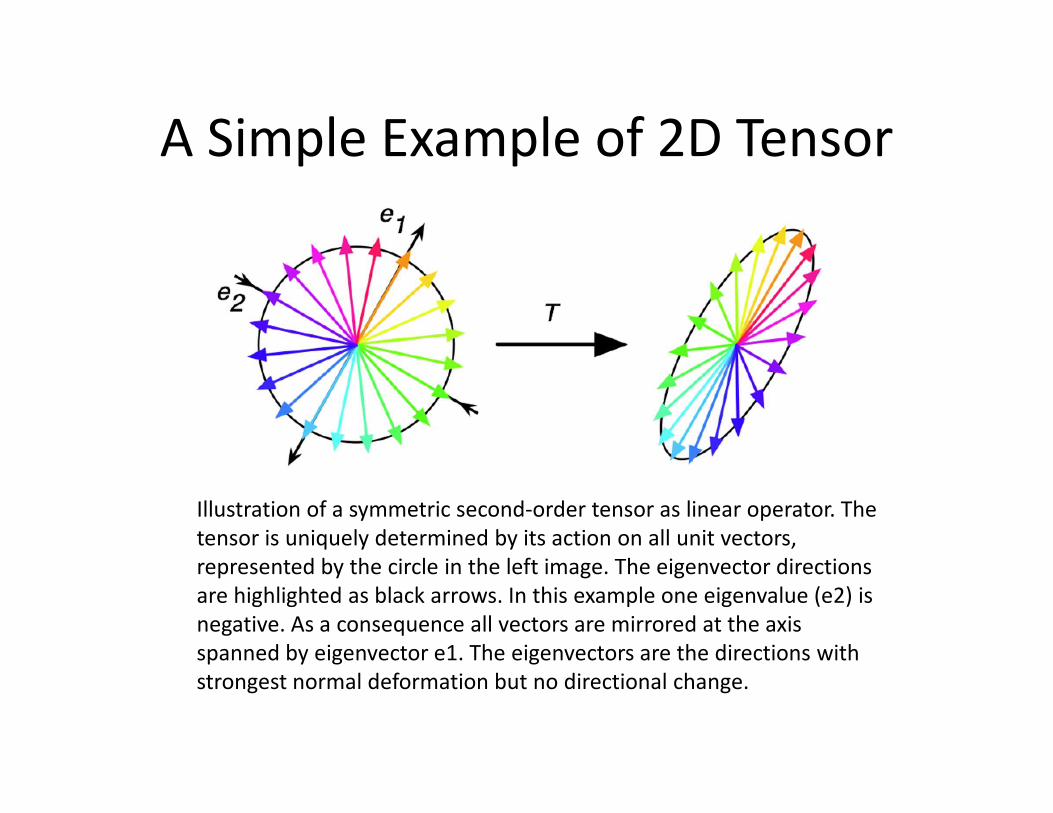
A Simple Example of 2D Tensor
Illustration of a symmetric second-order tensor as linear operator. The
tensor is uniquely determined by its action on all unit vectors,
represented by the circle in the left image. The eigenvector directions
are highlighted as black arrows. In this example one eigenvalue (e2) is
negative. As a consequence all vectors are mirrored at the axis
spanned by eigenvector e1. The eigenvectors are the directions with
strongest normal deformation but no directional change.
Applications
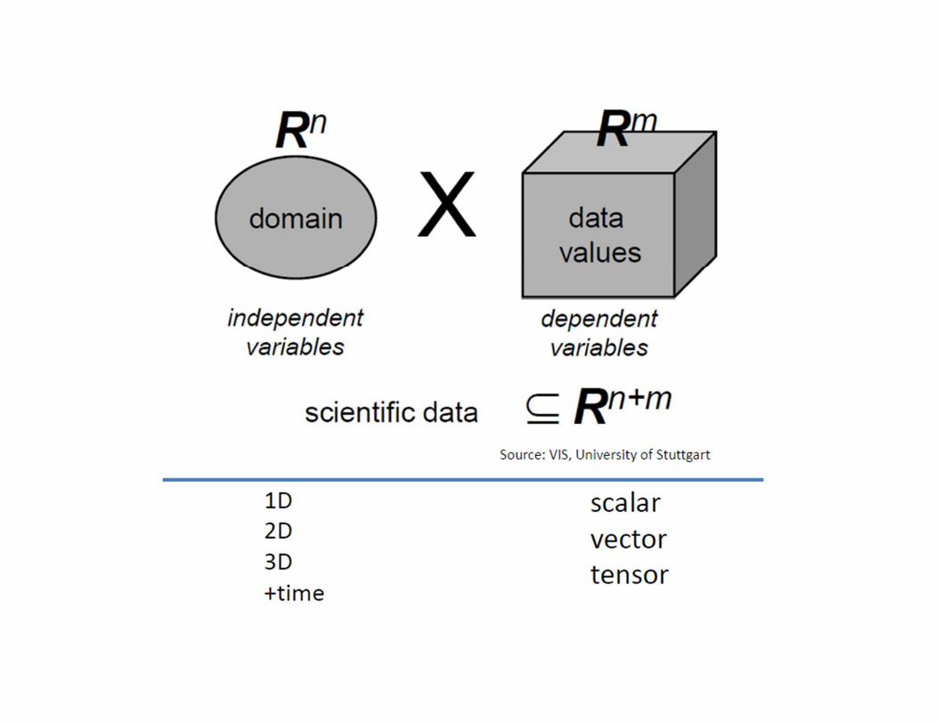
• Tensors describe entities that scalars and vectors cannot describe sufficiently, for example, the stress at a point in a continuous medium under load.
– medicine,
– geology,
– astrophysics,
– continuum mechanics
– and many more
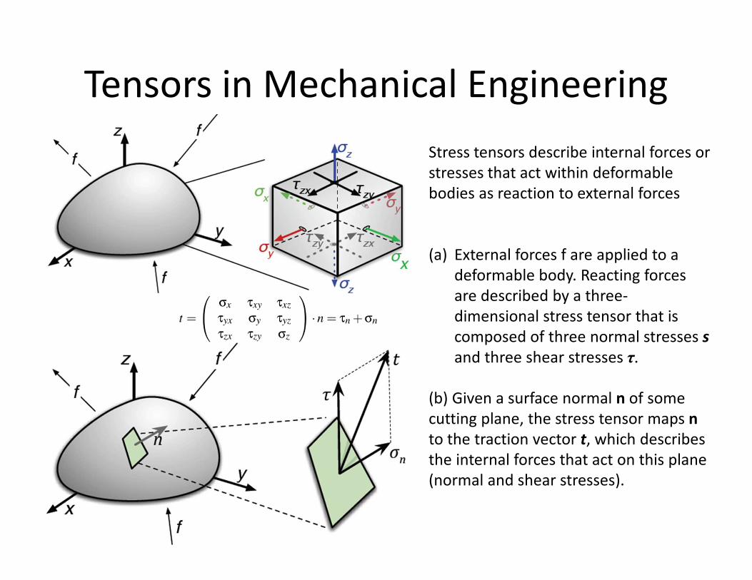
Stress tensors describe internal forces or
stresses that act within deformable
bodies as reaction to external forces
(a) External forces f are applied to a
deformable body. Reacting forces
are described by a three-
dimensional stress tensor that is
composed of three normal stresses s
and three shear stresses τ.
(b) Given a surface normal n of some
cutting plane, the stress tensor maps n
to the traction vector t, which describes
the internal forces that act on this plane
(normal and shear stresses).
Tensors in Mechanical Engineering
Tensors in Mechanical Engineering
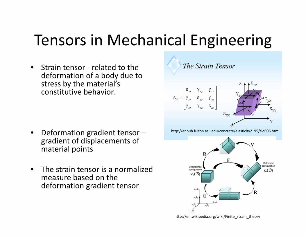
• Strain tensor - related to the deformation of a body due to stress by the material’s constitutive behavior.
• Deformation gradient tensor –gradient of displacements of material points
• The strain tensor is a normalized measure based on the deformation gradient tensor
http://enpub.fulton.asu.edu/concrete/elasticity2_95/sld006.htm
http://en.wikipedia.org/wiki/Finite_strain_theory
Diffusion Tensor Imaging (DTI)
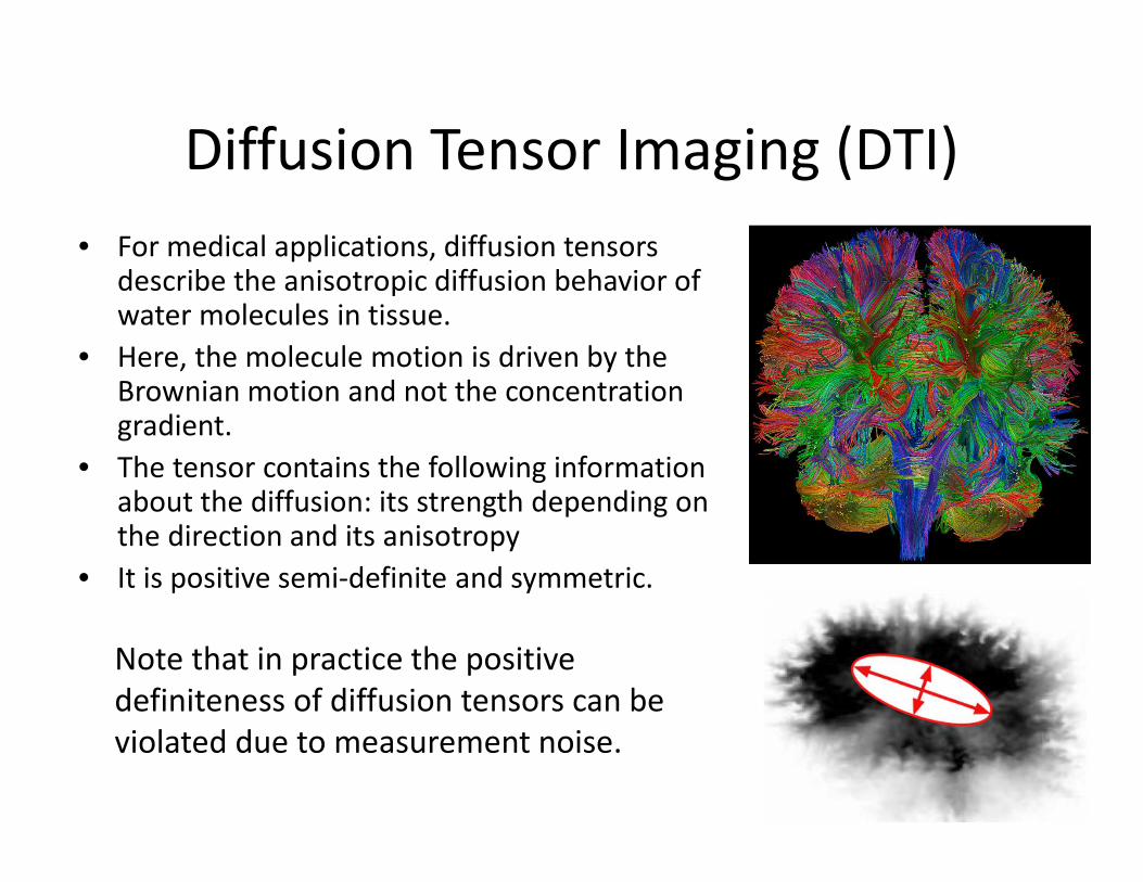
• For medical applications, diffusion tensors describe the anisotropic diffusion behavior of water molecules in tissue.
• Here, the molecule motion is driven by the Brownian motion and not the concentration gradient.
• The tensor contains the following information about the diffusion: its strength depending on the direction and its anisotropy
• It is positive semi-definite and symmetric.
Note that in practice the positive
definiteness of diffusion tensors can be
violated due to measurement noise.
Tensors in Medicine (II)
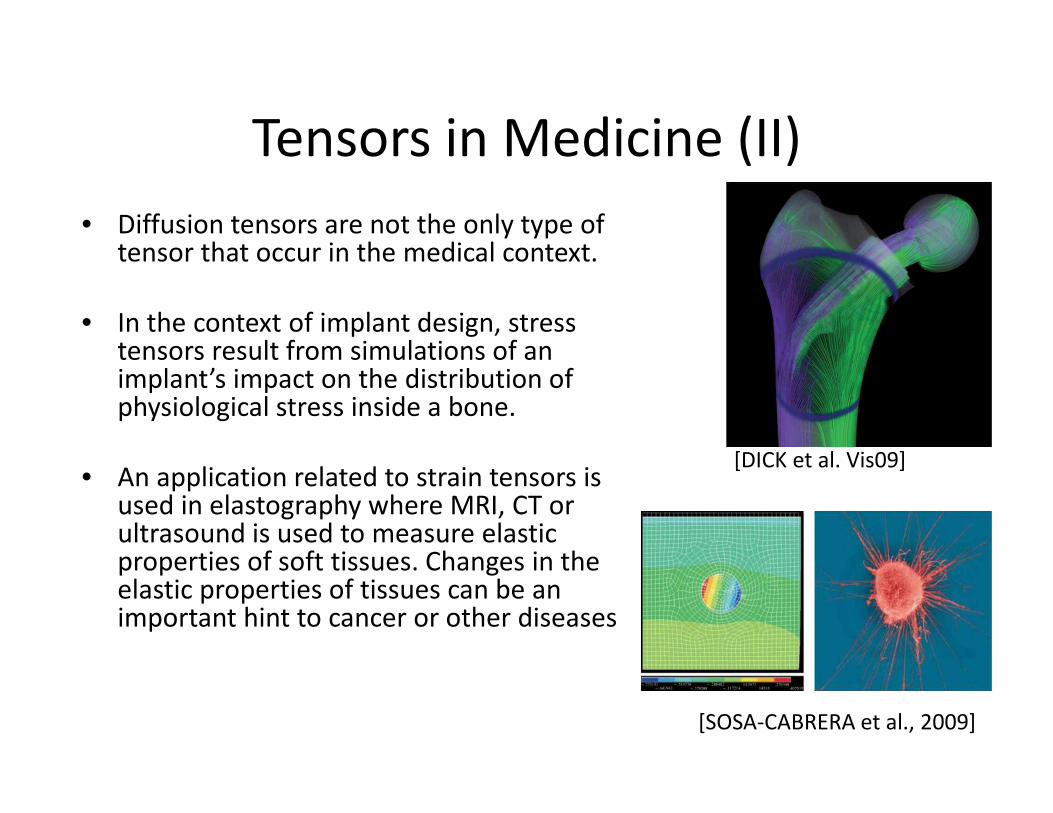
• Diffusion tensors are not the only type of tensor that occur in the medical context.
• In the context of implant design, stress tensors result from simulations of an implant’s impact on the distribution of physiological stress inside a bone.
• An application related to strain tensors is used in elastography where MRI, CT or ultrasound is used to measure elastic properties of soft tissues. Changes in the elastic properties of tissues can be an important hint to cancer or other diseases
[DICK et al. Vis09]
[SOSA-CABRERA et al., 2009]
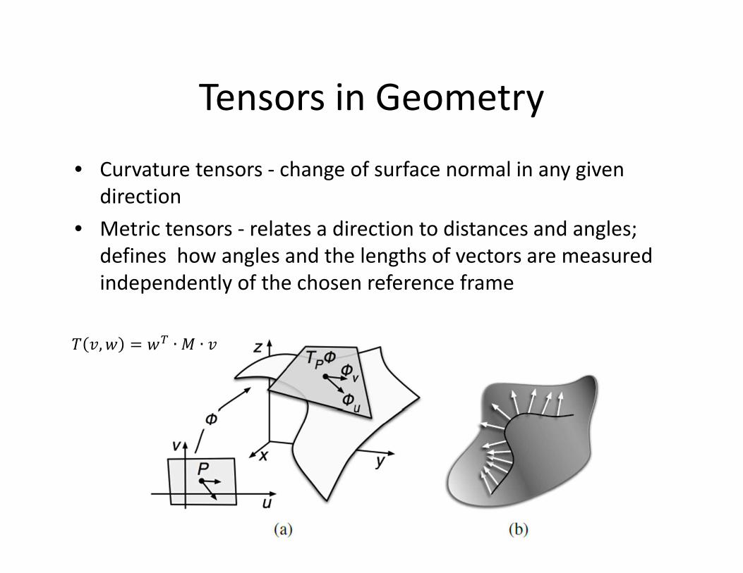
Tensors in Geometry
• Curvature tensors - change of surface normal in any given
direction
• Metric tensors - relates a direction to distances and angles;
defines how angles and the lengths of vectors are measured
independently of the chosen reference frame
� �,� � �� ∙ � ∙ �
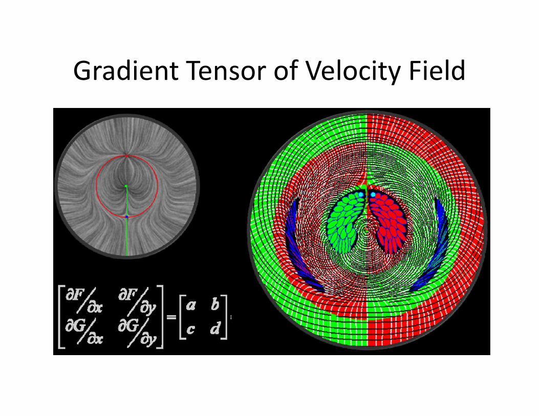
Gradient Tensor of Velocity Field
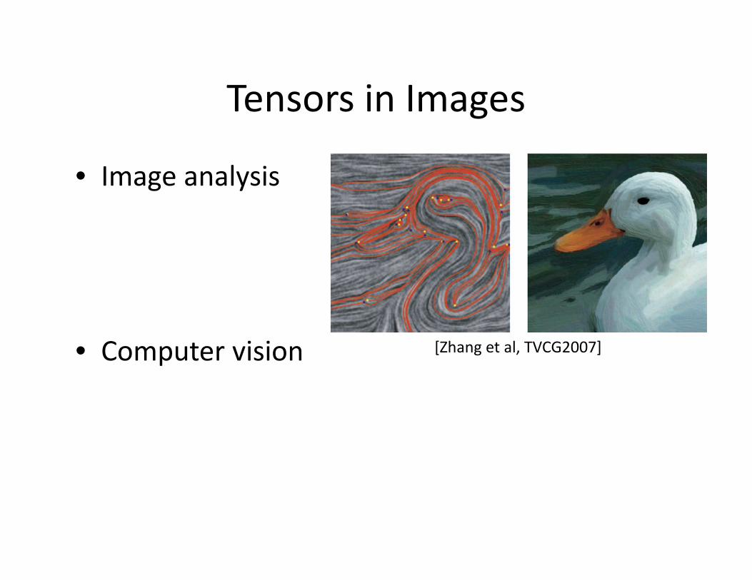
Tensors in Images
• Image analysis
• Computer vision [Zhang et al, TVCG2007]
Some Math of Tensors
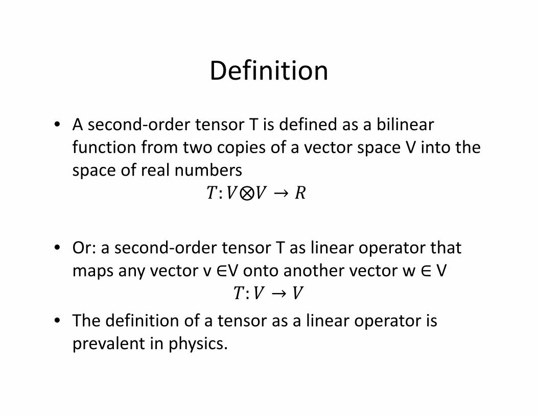
Definition
• A second-order tensor T is defined as a bilinear
function from two copies of a vector space V into the
space of real numbers
�: ⨂ →
• Or: a second-order tensor T as linear operator that
maps any vector v ∈V onto another vector w ∈V
�: →
• The definition of a tensor as a linear operator is
prevalent in physics.
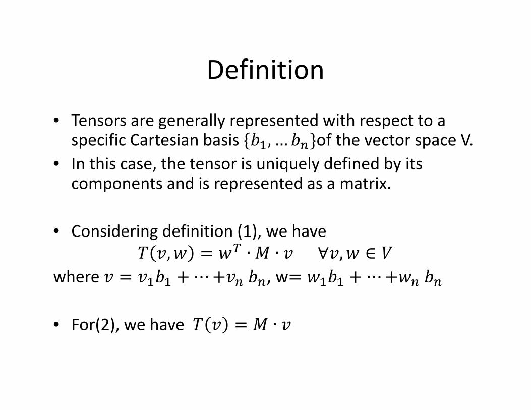
Definition
• Tensors are generally represented with respect to a specific Cartesian basis {��, … ��}of the vector space V.
• In this case, the tensor is uniquely defined by its components and is represented as a matrix.
• Considering definition (1), we have
� �,� � �� ∙ � ∙ �∀�, � ∈
where � � ���� + ⋯+�� ��, w� ���� + ⋯+�� ��
• For(2), we have � � � � ∙ �

Tensor Invariance
• Tensors are independent of specific reference frames, i.e. they are invariant under coordinate transformations.
• Invariance qualifies tensors to describe physical processes independent of the coordinate system. More precisely, the tensor components change according to the transformation into another basis; the characteristics of the tensor are preserved. Consequently, tensors can be analyzed using any convenient reference frame.
• Rotational invariant
• Affine invariant
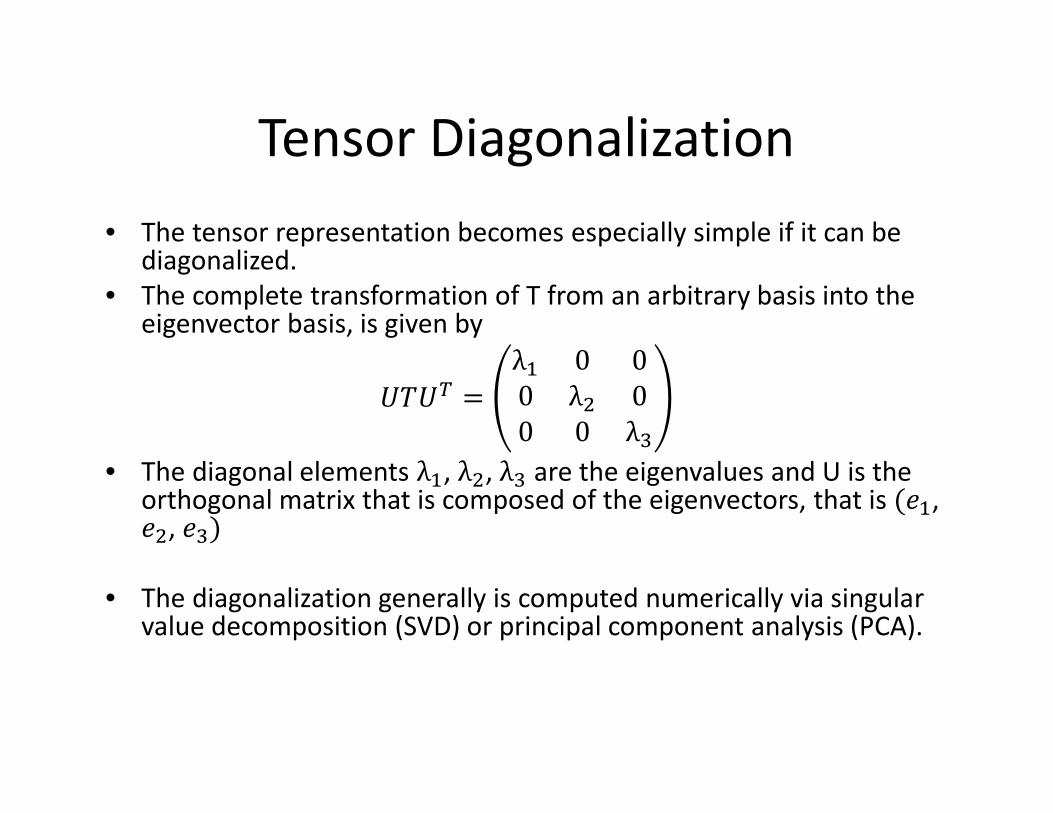
Tensor Diagonalization
• The tensor representation becomes especially simple if it can be diagonalized.
• The complete transformation of T from an arbitrary basis into the eigenvector basis, is given by
���� �
λ� 0 0
0 λ� 0
0 0 λ�
• The diagonal elements λ�, λ�, λ� are the eigenvalues and U is the orthogonal matrix that is composed of the eigenvectors, that is (��, ��, ��)
• The diagonalization generally is computed numerically via singular value decomposition (SVD) or principal component analysis (PCA).
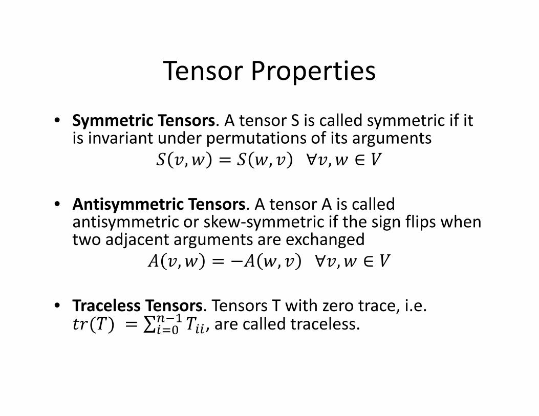
Tensor Properties
• Symmetric Tensors. A tensor S is called symmetric if it is invariant under permutations of its arguments
! �, � � ! �, � ∀�, � ∈
• Antisymmetric Tensors. A tensor A is called antisymmetric or skew-symmetric if the sign flips when two adjacent arguments are exchanged
" �,� � −" �, � ∀�, � ∈
• Traceless Tensors. Tensors T with zero trace, i.e. $%(�) � ∑ �''
�(�')* , are called traceless.
Tensor Properties
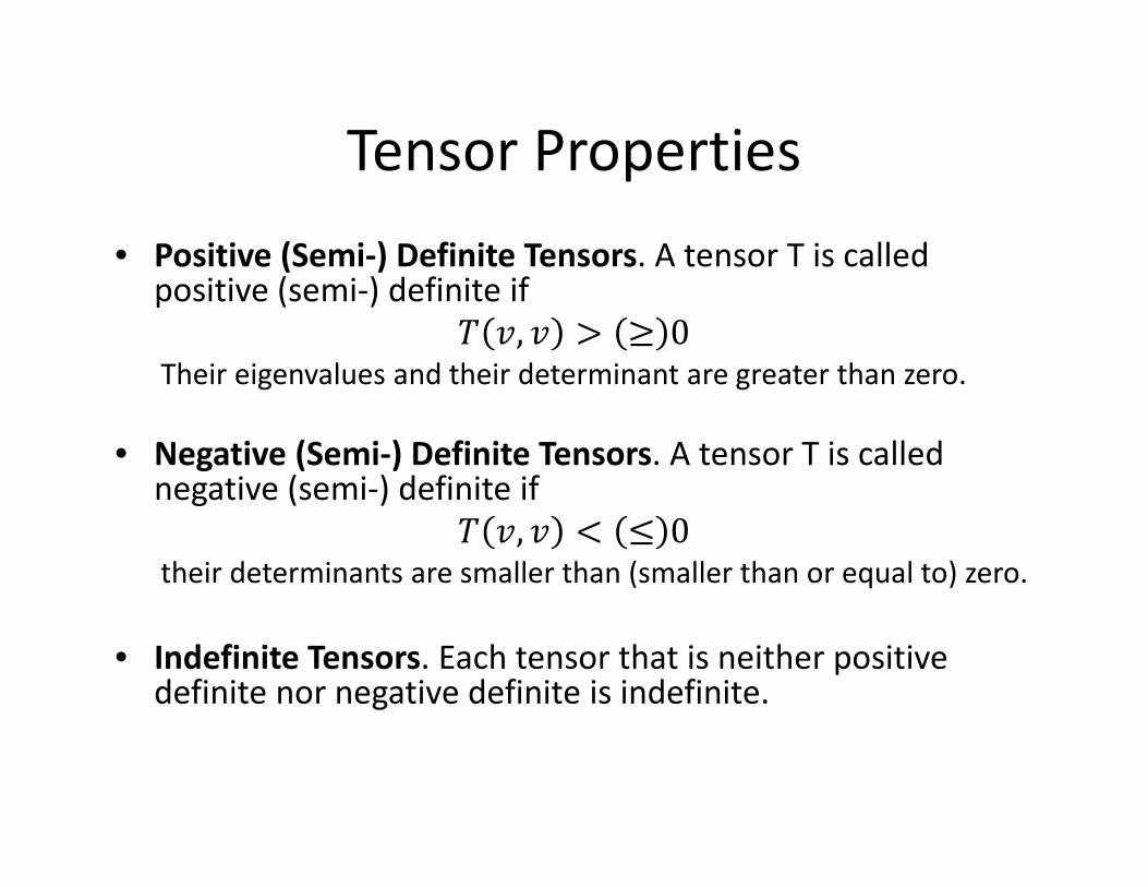
• Positive (Semi-) Definite Tensors. A tensor T is called positive (semi-) definite if
� �, � > ≥ 0Their eigenvalues and their determinant are greater than zero.
• Negative (Semi-) Definite Tensors. A tensor T is called negative (semi-) definite if
� �, � < ≤ 0their determinants are smaller than (smaller than or equal to) zero.
• Indefinite Tensors. Each tensor that is neither positive definite nor negative definite is indefinite.
Tensor Decompositions
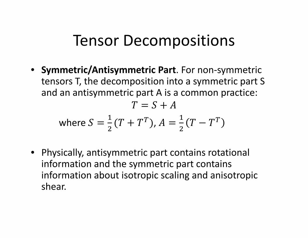
• Symmetric/Antisymmetric Part. For non-symmetric tensors T, the decomposition into a symmetric part S and an antisymmetric part A is a common practice:
� � ! + "
where ! ��
�(� + ��), " �
�
�� − ��
• Physically, antisymmetric part contains rotational information and the symmetric part contains information about isotropic scaling and anisotropic shear.
Tensor Decompositions
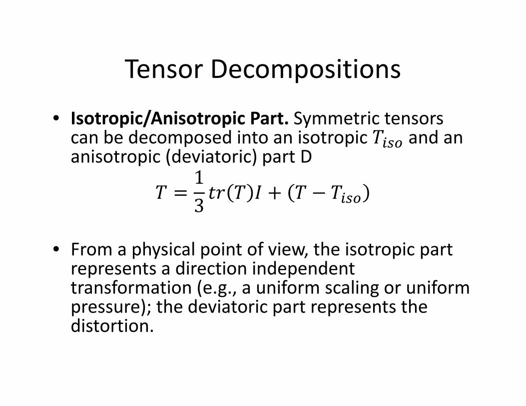
• Isotropic/Anisotropic Part. Symmetric tensors can be decomposed into an isotropic �'/0 and an anisotropic (deviatoric) part D
� �1
3$% � 3 + � − �'/0
• From a physical point of view, the isotropic part represents a direction independent transformation (e.g., a uniform scaling or uniform pressure); the deviatoric part represents the distortion.
Tensor Decompositions
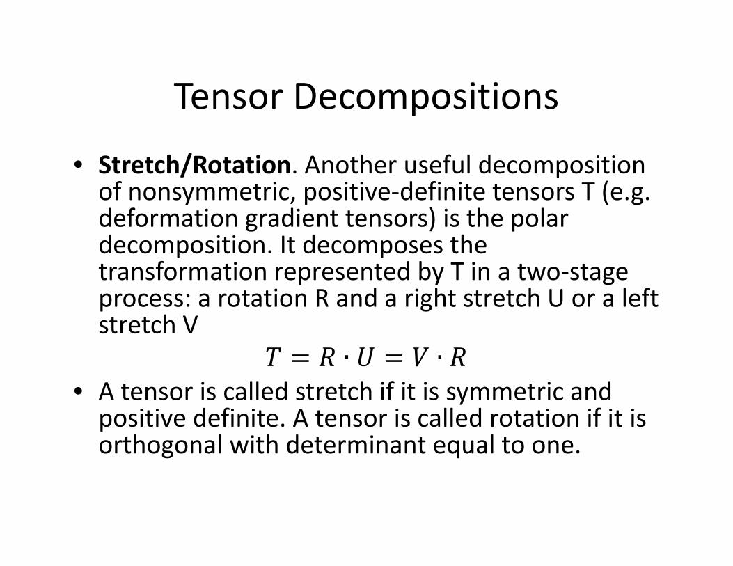
• Stretch/Rotation. Another useful decomposition of nonsymmetric, positive-definite tensors T (e.g. deformation gradient tensors) is the polar decomposition. It decomposes the transformation represented by T in a two-stage process: a rotation R and a right stretch U or a left stretch V
� � ∙ � � ∙
• A tensor is called stretch if it is symmetric and positive definite. A tensor is called rotation if it is orthogonal with determinant equal to one.
Tensor Decompositions
• Shape/Orientation. Via eigen analysis
symmetric tensors are separated into shape
and orientation.
– Here, shape refers to the eigenvalues and
orientation to the eigenvectors.
– Note that the orientation field is not a vector field
due to the bidirectionality of eigenvectors.
Second-order Tensor Fields
• In visualization, usually not only a single
tensor but a whole tensor field is of interest.
This gives rise to a tensor field.
Features?
• Scalar related
– Components
– Determinant
– Trace
– Eigen-values
• Vector related
– Eigen-vector fields
Tensor Interpolation
• Challenges– Natural representation of the original data.
• This includes the preservation of central tensor properties (e.g., positive definiteness) and/or important scalar tensor invariants (e.g., the determinant).
– Consistency. • consistent with the topology of the original data.
– Invariance. • The resulting interpolation scheme needs to be invariant with
respect to orthogonal changes of the reference frame.
– Efficiency. • The challenge is to design an algorithm that represents a tradeoff
between the above mentioned criteria and computational efficiency.

Tensor Interpolation
Comparison of component-wise tensor interpolation (a) and linear interpolation of eigenvectors
and eigenvalues (b). Observing the tensors depicted by ellipses, the comparison reveals that the
separate interpolation of direction and shape is much more shape-preserving (b).
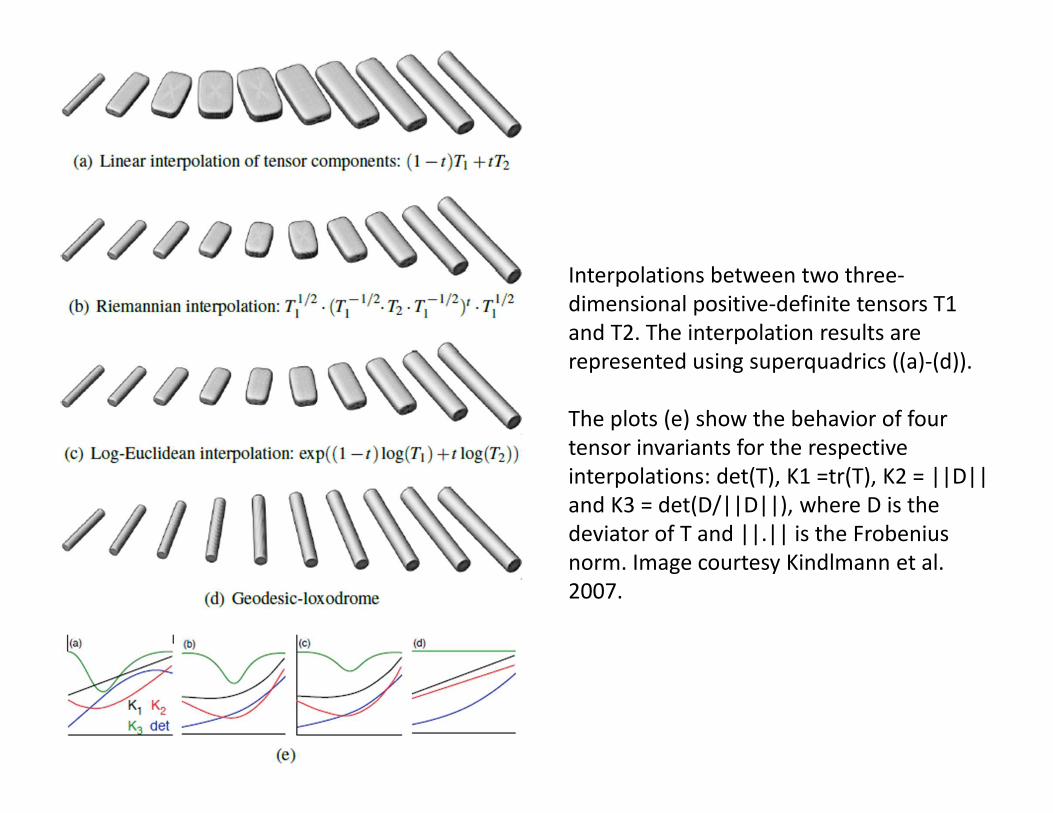
Interpolations between two three-
dimensional positive-definite tensors T1
and T2. The interpolation results are
represented using superquadrics ((a)-(d)).
The plots (e) show the behavior of four
tensor invariants for the respective
interpolations: det(T), K1 =tr(T), K2 = ||D||
and K3 = det(D/||D||), where D is the
deviator of T and ||.|| is the Frobenius
norm. Image courtesy Kindlmann et al.
2007.
Tensor Field Segmentation
• The goal of tensor segmentation algorithms is to aggregate regions that exhibit similar data characteristics to ease the analysis and interpretation of the data.
• Two classes
– Segmentation or clustering based on certain similarity (or dis-similarity) metric
– Topology-based

Tensor Field Segmentation
• Challenges– Similarity measure
• Depending on the task or visualization goal, a first step comprises the choice of appropriate quantities (derived features or original tensor data). These in turn influence or even determine the choice of an appropriate similarity measure.
– Simplification of complex structures• Topology-based segmentations may result in very complex
structures, which are hard to interpret. Therefore, algorithms for simplification and tracking over time play a crucial role.
• Topology higher than 2D is not well understood

Tensor Field Segmentation
• Similarity-Measure-Based Segmentation
– Based on tensor components, considering the
tensor segmentation as a multi-channel
segmentation of scalar values
– Based on invariants or comprise the entire tensor
data. Used metrics are the angular difference
between principal eigenvector directions, or
standard metrics considering the entire tensor,
like the Euclidean or Frobenius distance

What about tensor field topology?
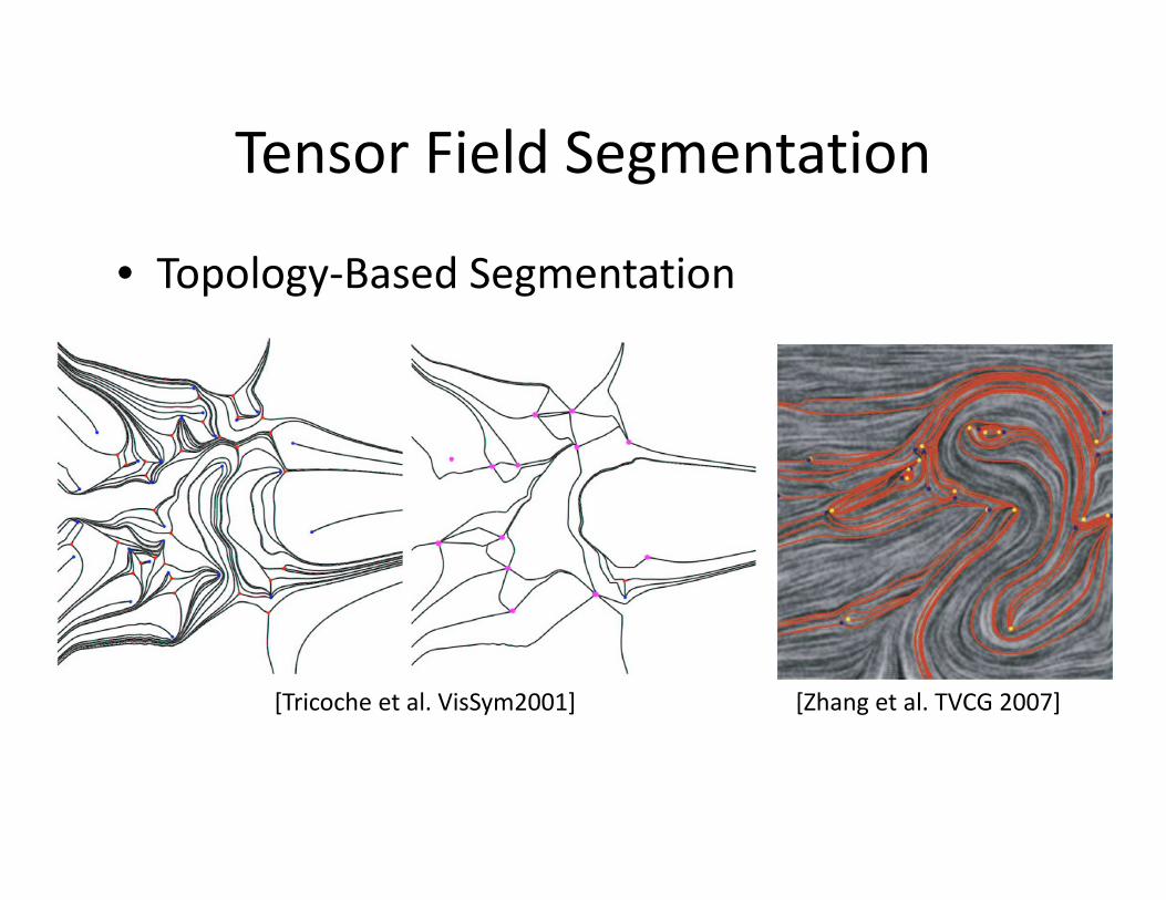
Tensor Field Segmentation
• Topology-Based Segmentation
[Tricoche et al. VisSym2001] [Zhang et al. TVCG 2007]
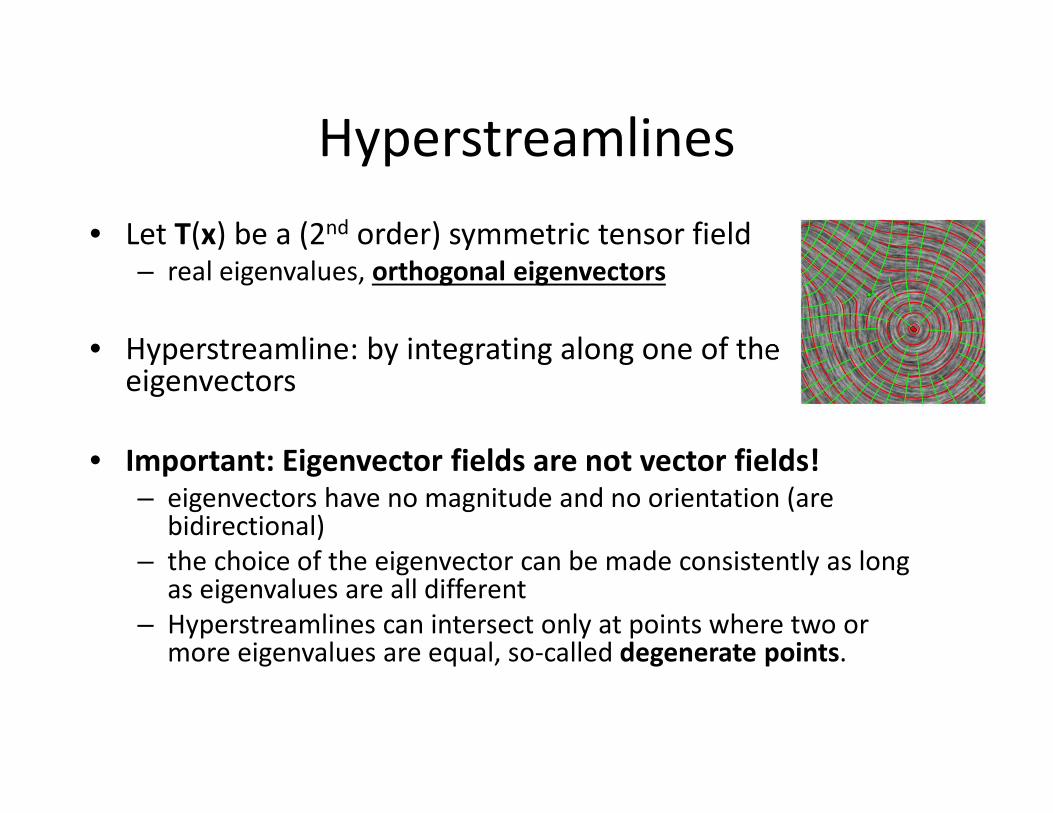
Hyperstreamlines
• Let T(x) be a (2nd order) symmetric tensor field– real eigenvalues, orthogonal eigenvectors
• Hyperstreamline: by integrating along one of the eigenvectors
• Important: Eigenvector fields are not vector fields!– eigenvectors have no magnitude and no orientation (are
bidirectional)
– the choice of the eigenvector can be made consistently as long as eigenvalues are all different
– Hyperstreamlines can intersect only at points where two or more eigenvalues are equal, so-called degenerate points.
Compute One Hyperstreamline
• Choose integrator:– Euler
– Runge-Kutta
• Choose step size (can be adaptive)
• Provide seed point position and determine starting direction
• Advance the front
• Note that the angle ambiguity. This is because the computation of the eigenvector at each sample point (i.e. vertex of the mesh) is independent of each other. Therefore, inconsistent directions may be chosen at neighboring vertices. – Additional step to remove angle ambiguity. A dot product between the
current advancing direction and the eigenvector direction at current position is performed. A positive value indicates the consistent direction; otherwise, the inverse direction should be used!
Degenerate Points
• The topology for 2nd symmetric tensor fields is extracted by identifying their degenerate points and their connectivity that partitions the hyperstreamlines.
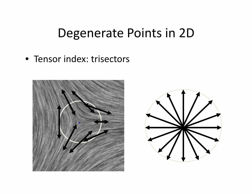
• A point p is a degenerate point of the tensor field T iff the two eigenvalues of T(p) are equal to each other. – There are infinite many eigenvectors at p.
– Hyperstreamlines cross each other at degenerate points
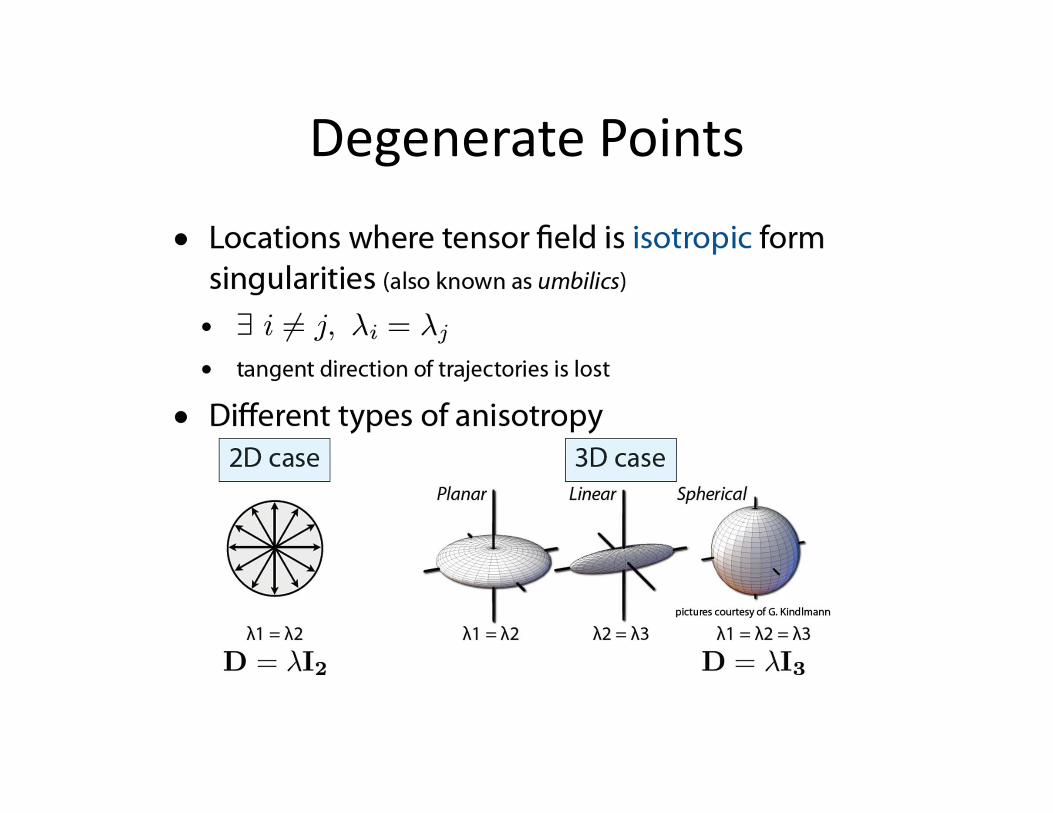
Degenerate Points
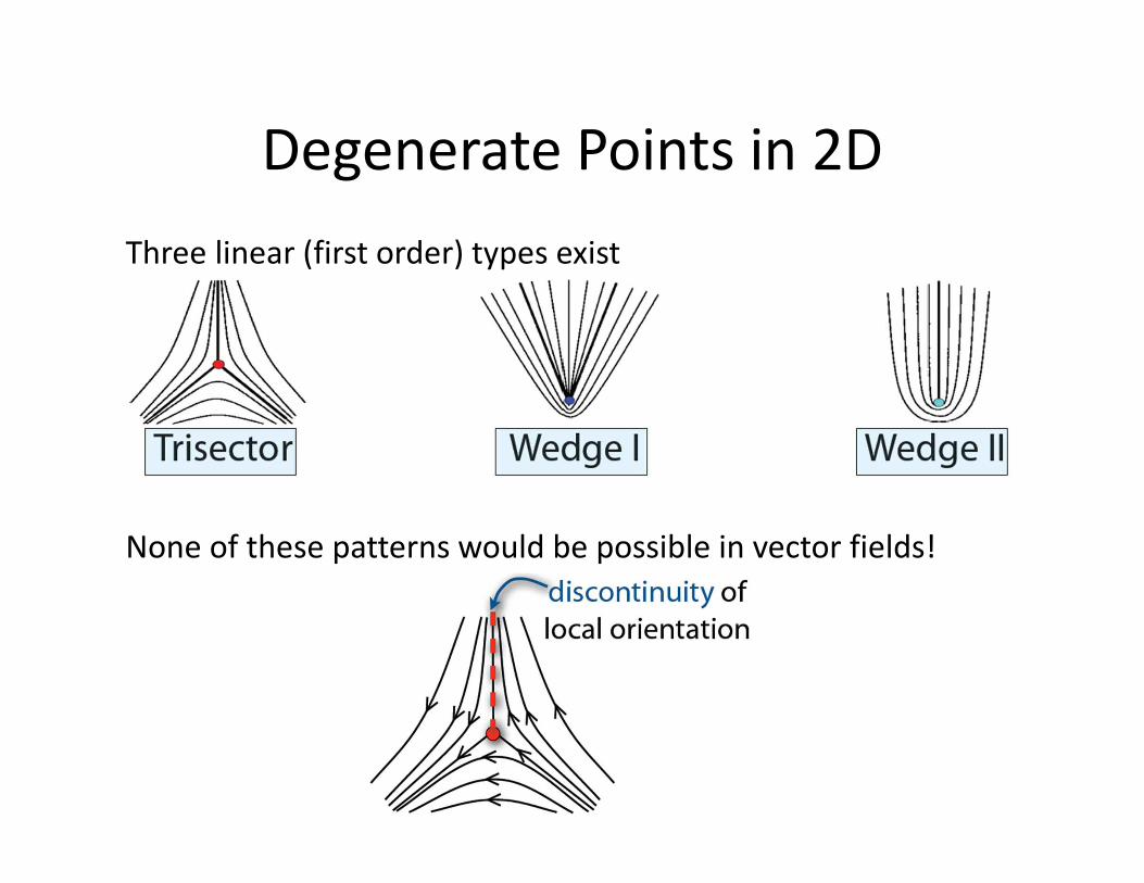
Degenerate Points in 2D
Three linear (first order) types exist
None of these patterns would be possible in vector fields!
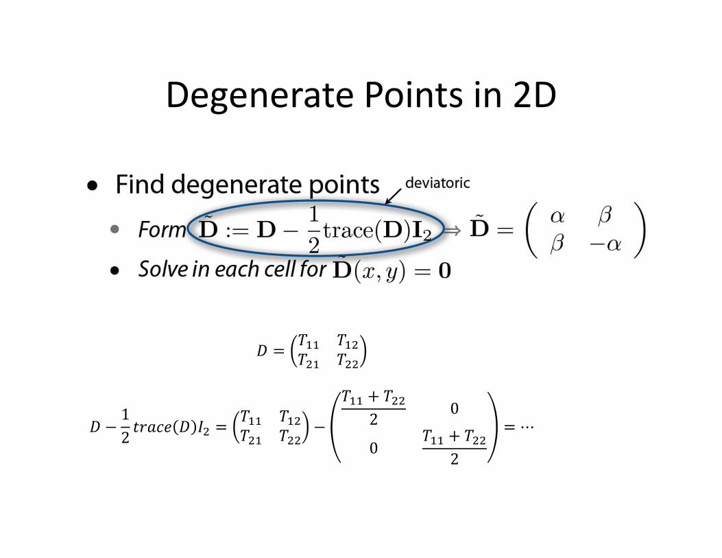
Degenerate Points in 2D
4 ���� ������ ���
4 −1
2$%67� 4 3� �
��� ������ ���
−
��� + ���
20
0��� + ���
2
� ⋯
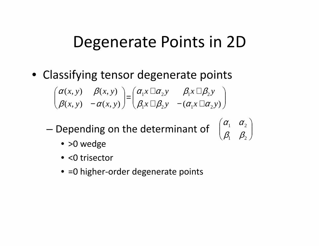
Degenerate Points in 2D
• Classifying tensor degenerate points
– Depending on the determinant of
• >0 wedge
• <0 trisector
• =0 higher-order degenerate points
+−+++
=
− )(),(),(
),(),(
2121
2121
yxyx
yxyx
yxyx
yxyx
ααββββαα
αββα
21
21
ββαα
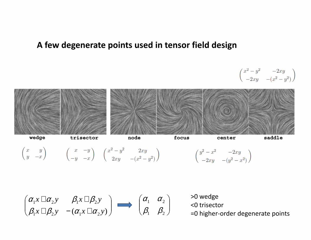
A few degenerate points used in tensor field design
>0 wedge
<0 trisector
=0 higher-order degenerate points
21
21
ββαα
+−+++
)( 2121
2121
yxyx
yxyx
ααββββαα
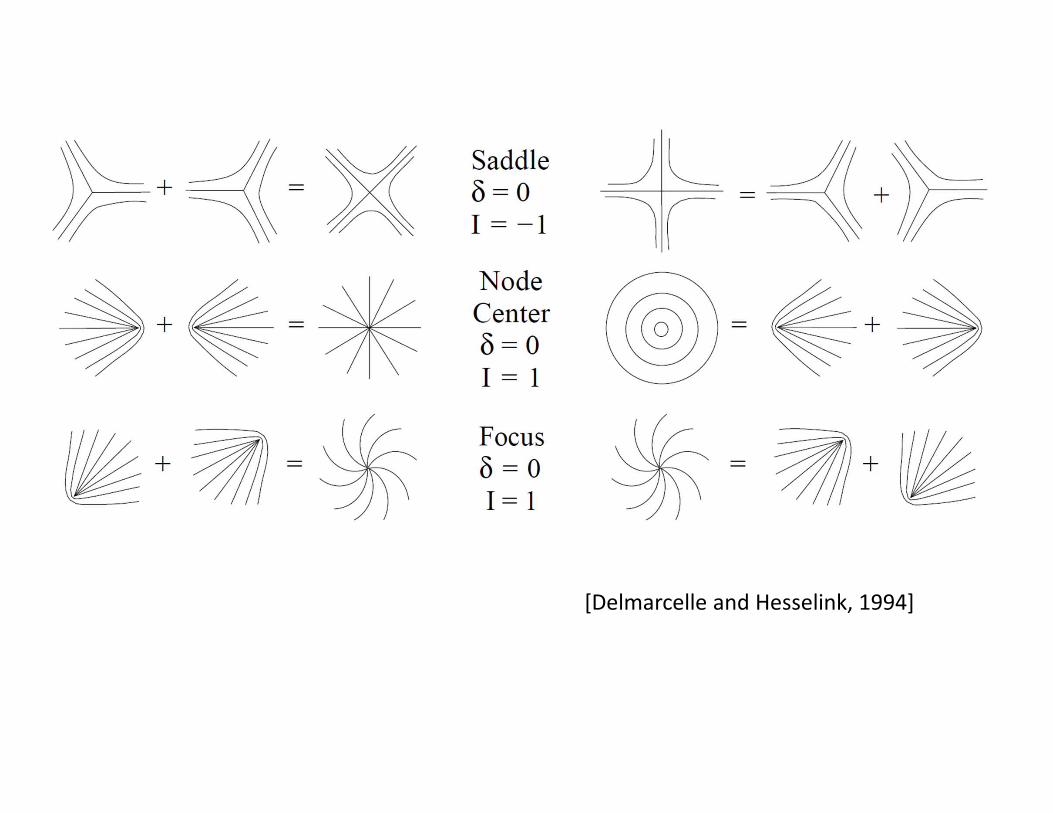
[Delmarcelle and Hesselink, 1994]

Degenerate Points in 2D
• Tensor index: wedges
Degenerate Points in 2D
• Tensor index: trisectors
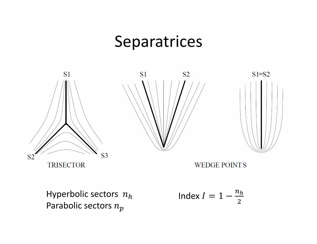
Separatrices
Hyperbolic sectors 89
Parabolic sectors 8:
Index 3 � 1 −�;
�
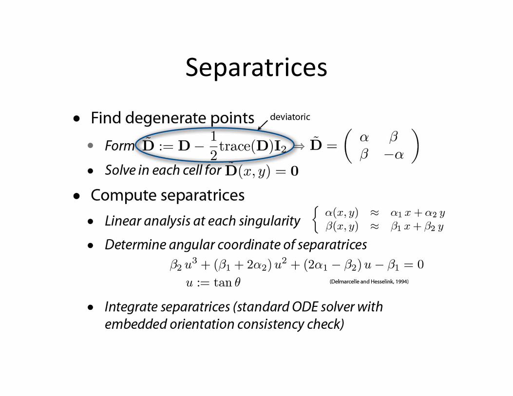
Separatrices
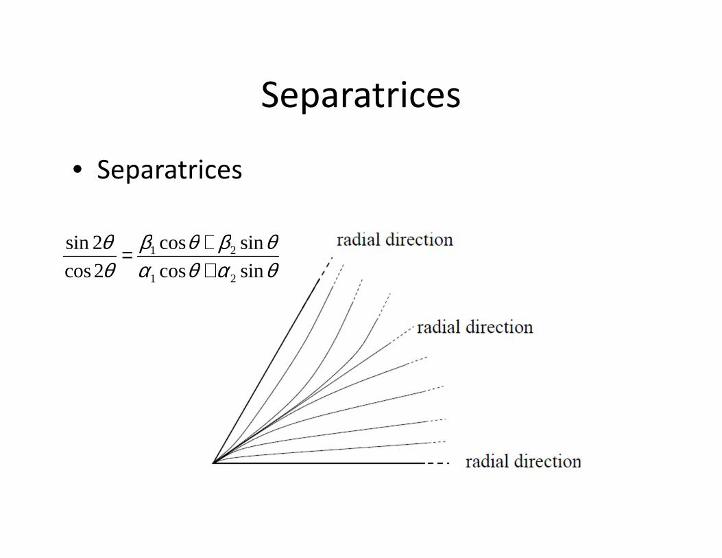
Separatrices
• Separatrices
θαθαθβθβ
θθ
sincos
sincos
2cos
2sin
21
21
++=
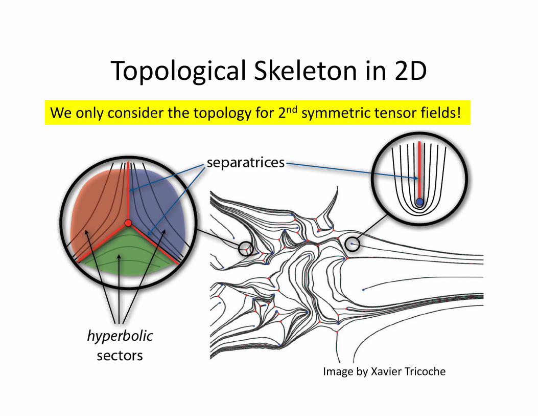
Topological Skeleton in 2D
Image by Xavier Tricoche
We only consider the topology for 2nd symmetric tensor fields!
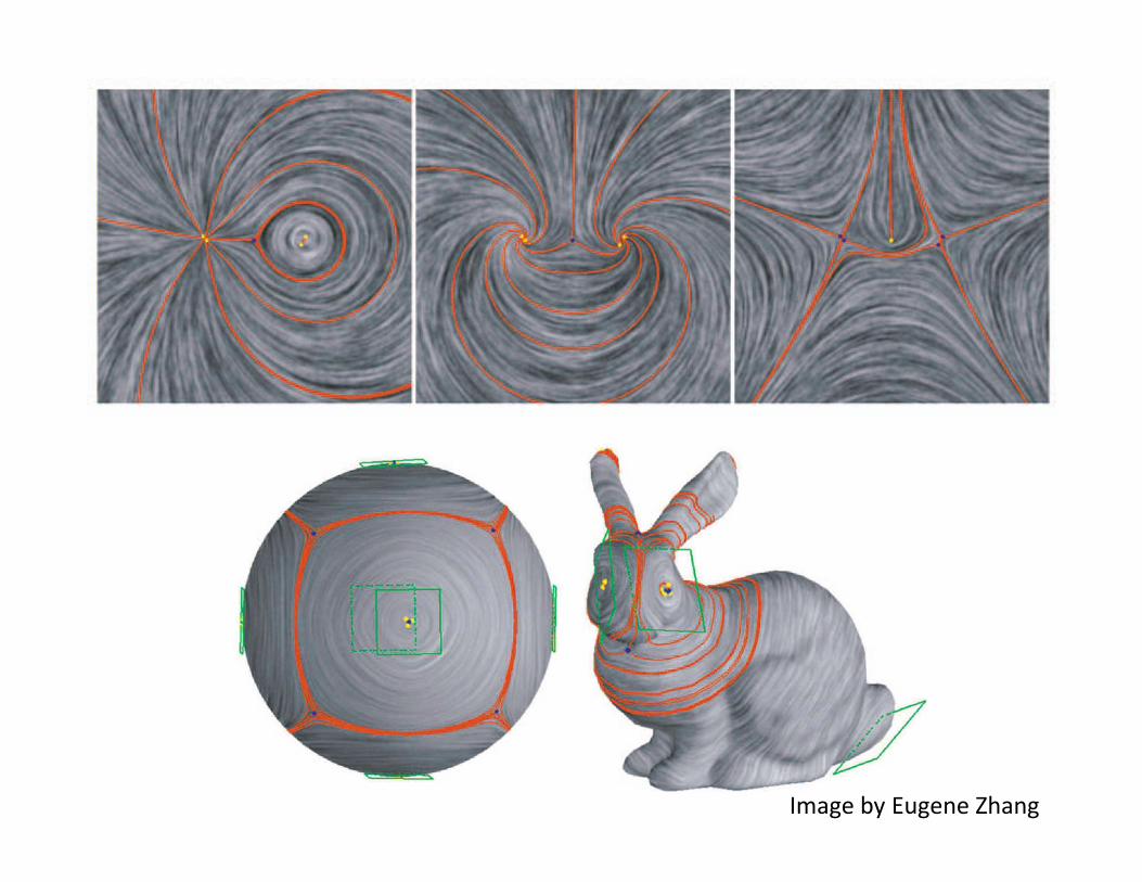
Image by Eugene Zhang
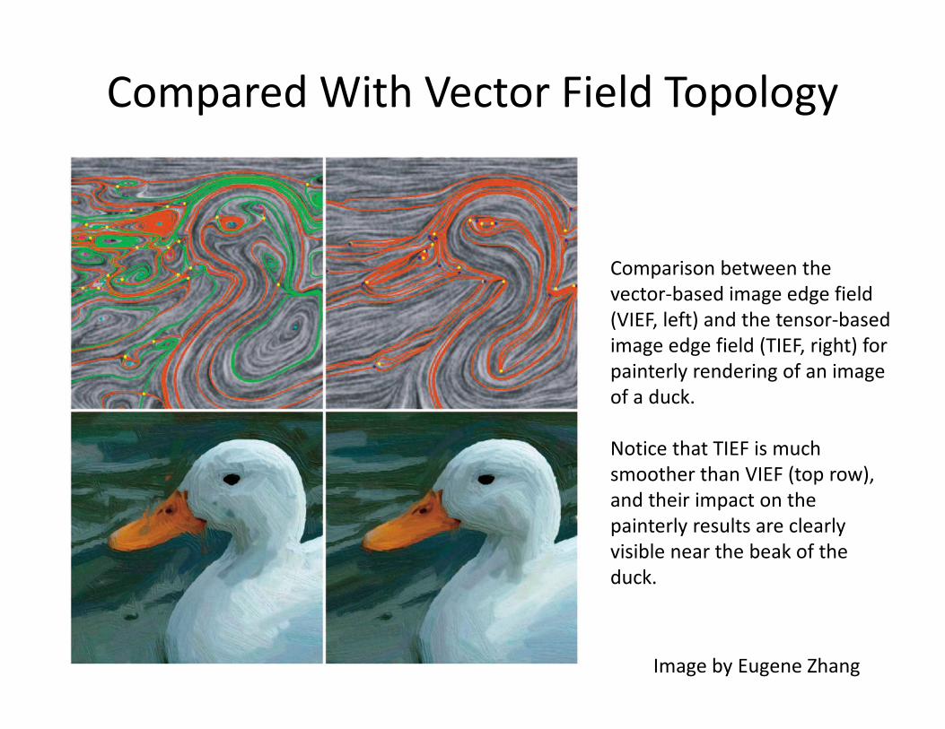
Compared With Vector Field Topology
Comparison between the
vector-based image edge field
(VIEF, left) and the tensor-based
image edge field (TIEF, right) for
painterly rendering of an image
of a duck.
Notice that TIEF is much
smoother than VIEF (top row),
and their impact on the
painterly results are clearly
visible near the beak of the
duck.
Image by Eugene Zhang
How about 3D topology?
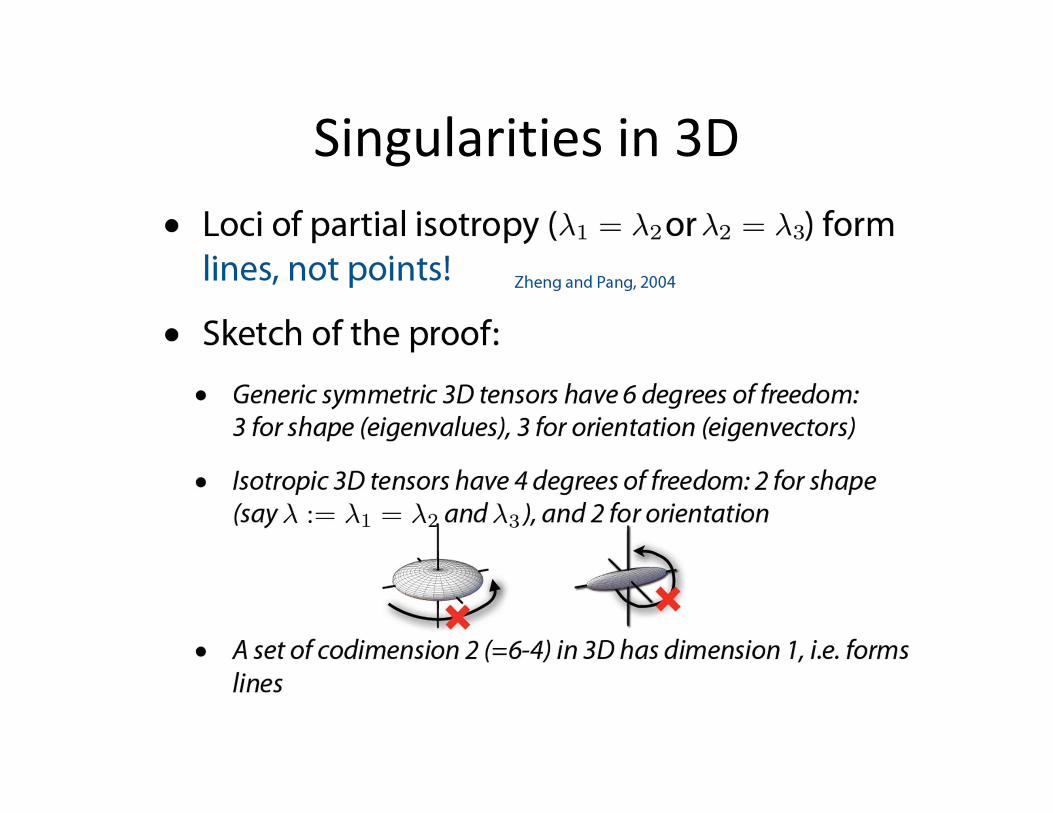
Singularities in 3D
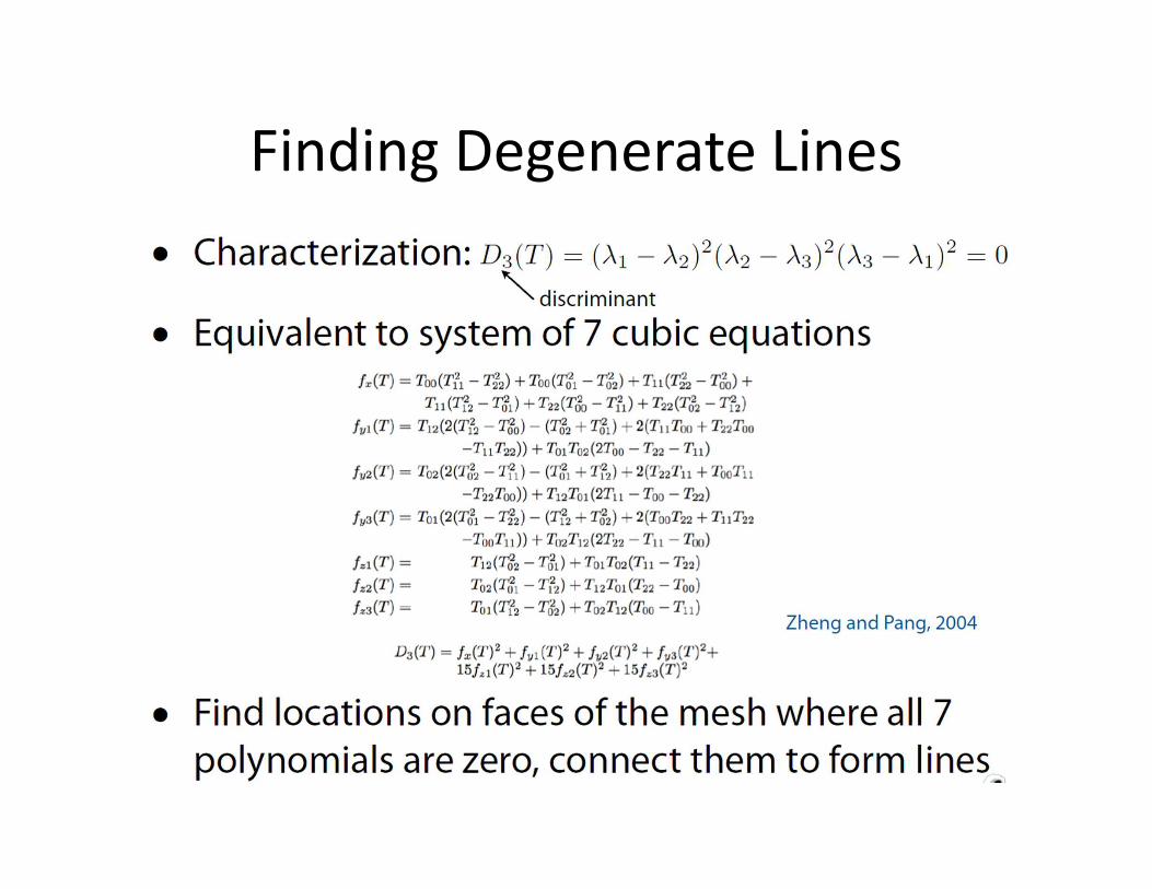
Finding Degenerate Lines

Finding Degenerate Lines
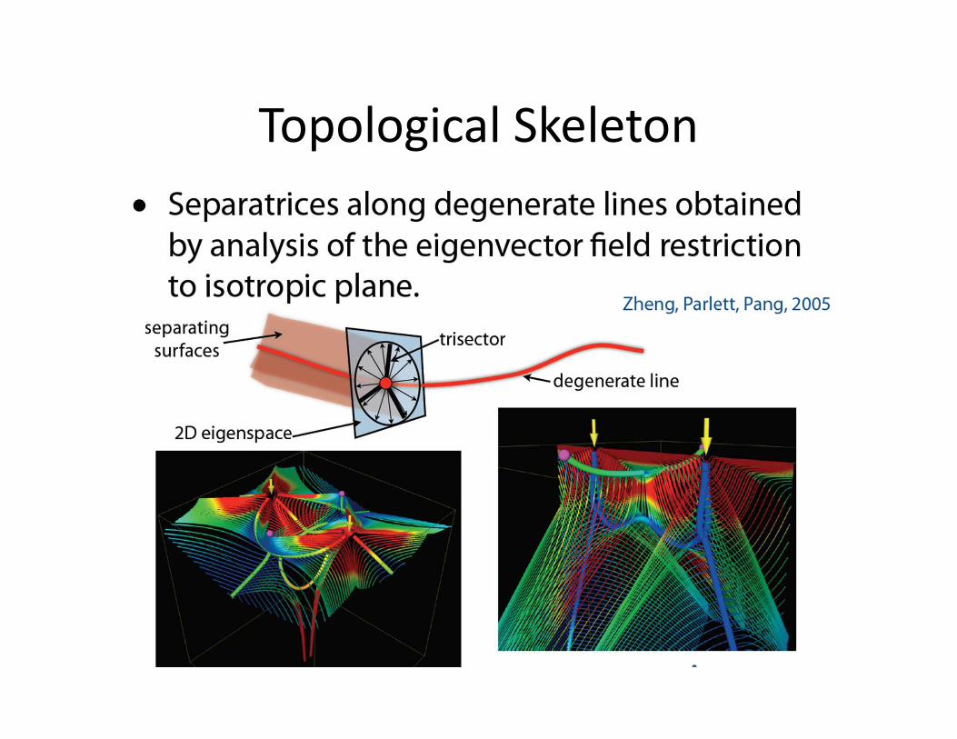
Topological Skeleton
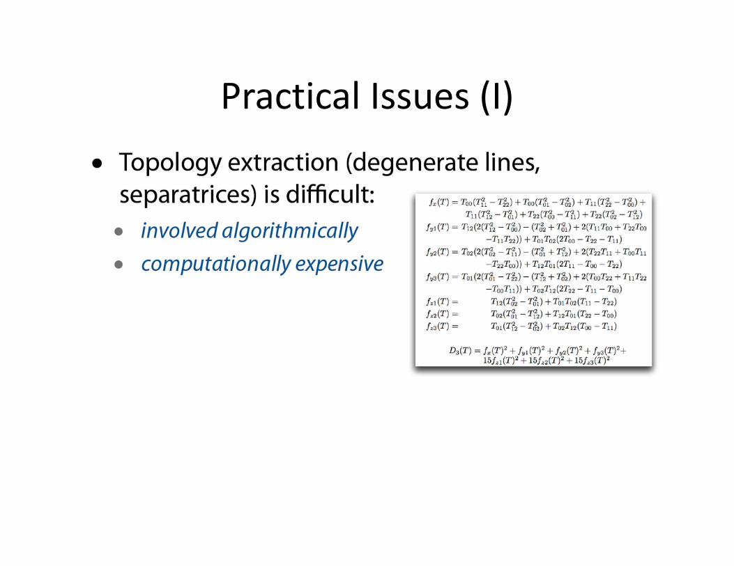
Practical Issues (I)
Time-dependent tensor field topology?
General tensor field topology?
Higher-order tensor field topology?
Acknowlegment
• Thanks material from
• Prof. Eugene Zhang, Oregon State University
• Prof. Xavier Tricoche, Purdue University
• And a survey paper
– Kratz, A.; Auer, C.; Stommel, M.; Hotz, I. Visualization
and Analysis of Second-Order Tensors: Moving Beyond
the Symmetric Positive-Definite Case. Computer
Graphics Forum - State of the Art Reports