teenagers' mode choice to and from school and technology

University of VermontScholarWorks @ UVM

Graduate College Dissertations and Theses Dissertations and Theses

2015

Teenagers' Mode Choice To And From SchoolAnd Technology Use For Transportation: AnalysisOf Students From Five High Schools In VermontAnd CaliforniaPaola Rekalde AizpuruUniversity of Vermont

Follow this and additional works at: https://scholarworks.uvm.edu/graddis

Part of the Civil Engineering Commons, and the Transportation Commons

This Thesis is brought to you for free and open access by the Dissertations and Theses at ScholarWorks @ UVM. It has been accepted for inclusion inGraduate College Dissertations and Theses by an authorized administrator of ScholarWorks @ UVM. For more information, please [email protected].

Recommended CitationRekalde Aizpuru, Paola, "Teenagers' Mode Choice To And From School And Technology Use For Transportation: Analysis OfStudents From Five High Schools In Vermont And California" (2015). Graduate College Dissertations and Theses. 481.https://scholarworks.uvm.edu/graddis/481

https://scholarworks.uvm.edu?utm_source=scholarworks.uvm.edu%2Fgraddis%2F481&utm_medium=PDF&utm_campaign=PDFCoverPages

https://scholarworks.uvm.edu/graddis?utm_source=scholarworks.uvm.edu%2Fgraddis%2F481&utm_medium=PDF&utm_campaign=PDFCoverPages

https://scholarworks.uvm.edu/etds?utm_source=scholarworks.uvm.edu%2Fgraddis%2F481&utm_medium=PDF&utm_campaign=PDFCoverPages

https://scholarworks.uvm.edu/graddis?utm_source=scholarworks.uvm.edu%2Fgraddis%2F481&utm_medium=PDF&utm_campaign=PDFCoverPages

http://network.bepress.com/hgg/discipline/252?utm_source=scholarworks.uvm.edu%2Fgraddis%2F481&utm_medium=PDF&utm_campaign=PDFCoverPages

http://network.bepress.com/hgg/discipline/1068?utm_source=scholarworks.uvm.edu%2Fgraddis%2F481&utm_medium=PDF&utm_campaign=PDFCoverPages

https://scholarworks.uvm.edu/graddis/481?utm_source=scholarworks.uvm.edu%2Fgraddis%2F481&utm_medium=PDF&utm_campaign=PDFCoverPages

mailto:[email protected]

TEENAGERS’ MODE CHOICE TO AND FROM SCHOOL AND

TECHNOLOGY USE FOR TRANSPORTATION: ANALYSIS OF

STUDENTS FROM FIVE HIGH SCHOOLS IN VERMONT AND

CALIFORNIA

A Thesis Presented

by

Paola Rekalde Aizpuru

to

The Faculty of the Graduate College

of

The University of Vermont

In Partial Fulfillment of the Requirements

for the Degree of Master of Science

Specializing in Civil and Environmental Engineering

October, 2015

Defense Date: June 30, 2015

Thesis Examination Committee:

Brian H.Y. Lee, Ph.D, Advisor

Meghan Cope, Ph.D, Chairperson

Lisa Aultman-Hall, Ph.D.

Cynthia J. Forehand, Ph.D., Dean of the Graduate College

ABSTRACT

The carhops and drive-ins of the 1950s are symbolic of the freedom that the

automobile has granted Americans. What the general public has gained from the

automobile, however, may come at the expense of independent mobility and choices for

today’s adolescents, particularly those not yet old enough to drive or those from lower

income families. Sprawl land use development patterns and limited transportation choices

in most American cities often hold teenagers and their chauffeuring parents captive to the

automobile. At the same time, information and communication technology is fast

evolving and changing the ways in which teenagers live, interact, and communicate with

others; easier transportation coordination is one potential outcome. This study seeks to

examine teenagers’ travel behavior for their most common destination – going to and

from school – and how the use of technology influences this behavior. Survey data from

five high schools, three in Northern California and two in Vermont, are used to identify

the mode choice to and from school, socio-demographic characteristics, and technology

use of the sampled teenagers. The built environment of the teenagers’ home surroundings

is determined by data obtained from the 2010 Census. Logistic regression analysis is used

to describe the most significant variables influencing both mode choice to and from

school, and the factors associated with the use of technology. Those variables with a

family income component, such as high family education, access to a car and smartphone

ownership have a positive effect on teenagers driving more to and from school. Similarly,

those teens who travel longer distances depend more on rides and choose active modes of

transportation than teens living in more populated neighborhoods. When it comes to

technology use for transportation among teenagers, those living farther away from

school, in worse connected neighborhoods are more likely to depend more on technology

for arranging transportation, whereas those teens who choose active transportation modes

to school depend less on. High density development policies seem the right

recommendation to ensure teenagers choose active transportation alternatives to school

and depend less on their parents, family, and friends to move around. Due to the strong

influence of attitudes in teenagers’ behavior, social education and culture adaptation

programs could be suggested to encourage teens to become more confident on active

transportation modes, as well as promote safe routes to school for both genders.

ii

TABLE OF CONTENTS

LIST OF TABLES ........................................................................................................... v

LIST OF FIGURES ....................................................................................................... vii

CHAPTER 1 – Introduction ............................................................................................ 1

Motivations ...................................................................................................................... 3

CHAPTER 2 – LITERATURE REVIEW ....................................................................... 7

Socio-Demographic characteristics .............................................................................. 8

Attitudes ...................................................................................................................... 10

Built environment characteristics ............................................................................... 12

Virtual environment .................................................................................................... 15

CHAPTER 3 – DATA ................................................................................................... 18

Survey Data.................................................................................................................... 18

Origin and school environment description ................................................................ 18

Study from the University of Vermont ..................................................................... 18

Study of Northern California .................................................................................... 22

Geographic Data ............................................................................................................ 25

Descriptive Statistics...................................................................................................... 27

iii

Data Processing.............................................................................................................. 34

Data analysis ............................................................................................................... 35

CHAPTER 4 – MODE CHOICE TO AND FROM SCHOOL ..................................... 43

Statistical method ........................................................................................................... 43

Modeling mode choice................................................................................................... 44

Results and discussion ................................................................................................... 45

Model 4.1: Combined California and Vermont High Schools Model ........................ 46

Model 4.2: California High Schools Model ............................................................... 50

Model 4.3: California High Schools Model with attitudinal variables ....................... 53

Conclusions .................................................................................................................... 59

CHAPTER 5 – TECHNOLOGY USE FOR TRANSPORTATION ............................. 61

Statistical method ........................................................................................................... 61

Modeling technology use for transportation .................................................................. 62

Results and discussion ................................................................................................... 63

Model 5.1: Frequency of technology use for transportation arrangement, all five high

schools ........................................................................................................................ 64

Model 5.2: Frequency of technology use for transportation arrangement, California 66

iv

Model 5.3: Frequency of technology use for transportation arrangements plus

attitudinal factors, California ...................................................................................... 67

Conclusions .................................................................................................................... 71

CHAPTER 6 .................................................................................................................. 73

Summary ........................................................................................................................ 73

Limitations ..................................................................................................................... 76

Recommendations .......................................................................................................... 77

REFERENCES .............................................................................................................. 80

v

LIST OF TABLES

Page

Table 1 Socio-demographic attributes of the two high school

locations in Vermont .......................................................................................... 22

Table 2 Socio-demographic attributes of the three high school

locations in California ........................................................................................ 25

Table 3 Mode choice proportion per high school .............................................. 28

Table 4 Geocoding percentages and matches per high school .......................... 34

Table 5 Survey variables recoding ..................................................................... 36

Table 6 Geographical data variables .................................................................. 40

Table 7 Distance Descriptive Statistics ............................................................. 40

Table 8 Population density (total and teenager) by distance buffers.

Descriptive Statistics. ......................................................................................... 41

Table 9 Street length descriptive statistics by distance buffers ......................... 41

Table 10 Distribution of transportation mode for daily commute by

census tract (%) .................................................................................................. 41

Table 11 Distribution of Occupations by census tract (%) ................................ 41

Table 12 Mode to school Nominal Logistic Regression model results

(Five high schools) ............................................................................................. 46

Table 13 Mode to school Nominal Logistic Regression model results

(California high schools) .................................................................................... 51

Table 14 Mode to school Nominal Logistic Regression model

results, plus attitudinal factors (California high schools) ................................... 54

vi

Table 15 Technology use for transportation arrangements, five high schools .. 65

Table 16 Technology use for transportation, California .................................... 67

Table 17 Technology use for transportation plus attitudinal factors,

California ............................................................................................................ 69

vii

LIST OF FIGURES

Page

Figure 1 Location of the State of Vermont ........................................................ 20

Figure 2 Location of Chittenden county and SBHS and CVUHS ..................... 21

Figure 3 Locations of Davis, Tamalpais, and Sequoia high schools in

Northern California ............................................................................................ 23

Figure 4 Mode choice by grade in South Burlington High School ................... 28

Figure 5 Mode choice by grade in Champlain Valley Union High School ....... 29

Figure 6 Mode choice by grade in Sequoia High School .................................. 30

Figure 7 Mode choice by gender South Burlington High School ..................... 31

Figure 8 Mode choice by gender Champlain Valley Union High School ......... 31

Figure 9 Mode choice by gender DAVIS .......................................................... 32

Figure 10 Mode choice by gender TAMALPAIS ............................................. 32

Figure 11 Mode choice by gender SEQUOIA ................................................... 33

Figure 12 Bicycle Distribution .......................................................................... 37

Figure 13 Phone Distribution ............................................................................ 37

Figure 14 Technology Use Distribution ............................................................ 38

Figure 15 Driving License Distribution ............................................................. 38

Figure 16 Education Distribution ...................................................................... 39

Figure 17 Siblings Distribution ......................................................................... 39

Figure 18 Distance to School Distribution by buffers ....................................... 40

1

CHAPTER 1 – Introduction

The carhops and drive-ins of the 1950s are symbolic of the freedom that the

automobile has granted America’s youth. Having the choice to drive, walk, or bike to a

particular destination, however, is a privilege that not every teenager can enjoy. What the

general public has gained from the automobile may come at the expense of independent

mobility and choices for today’s adolescents, particularly those not yet old enough to

drive, or those from lower income families who cannot afford or do not have access to

this mode. Income and other socio-demographic characteristics of families often define

the accessibility of teenaged users to certain modes and, therefore, may affect their daily

transportation routine. Public transit and other alternative modes may have the potential

to offer greater autonomy for teenagers. However, sprawling land use development

patterns as well as the limited transportation choices in most American cities may hold

teenagers and their chauffeuring parents captive to the private automobile. These built

environment characteristics may be some of the factors that influence American

teenagers’ choice of mode to commute to school.

Also, technology is evolving faster and faster. The internet has become a widely

used tool especially in developed countries. A large majority of individuals in the country

have access to the web and use it not only for business (File and Ryan 2014), browsing or

even playing, but also for communicating with other individuals. In addition, the

improvements that have been developed around mobile devices and tablets have been

shown to increase the use of these devices at an individual user scale. Phone calls, texts,

emails, online chatting, and social media are part of present day teenager’s everyday life

2

(Craig, McInroy et al. 2014). We might not realize, but we use smartphones and

computers in our everyday lives, and these technologies are making a difference in the

way we live, interact and communicate with others. Teenagers have grown up using these

technologies, and therefore they are part of their daily routine. In fact, according to Pew

Internet and American Life project (2013) 95 % of adolescents (12–17) and 94 % of

young adults (18–29) in the United States were online in 2011, and are more likely than

adults to communicate using information and communication technologies (ICTs). This

increase in communication alternatives for young populations may affect their way of

arranging transportation. Being in constant communication with family members and

friends may improve their transportation options and alternatives, increasing the number

of activities they can access to. The use of technology for transportation related

arrangements may make a change in the travel behavior of teenagers.

With this study, I seek to examine teenagers’ travel behavior for their most

common trip – going to and from school – and also factors related to their use of

technology for their general transportation needs. Survey data from five high schools in

the U.S. has been used in the study, two from Vermont and three from Northern

California. Such surveys, developed and conducted by researchers at the University of

Vermont and University of California Davis, were not the same for both states but had

many questions in common. The California survey included questions related to

teenagers’ attitude towards transportation, which allowed for examinations of those

factors. In addition to the survey data, geographical data analysis has also been developed

to better define the built environment characteristics.

3

Specifically, the paper sets out to explore the following questions:

- What factors influence teenagers’ travel mode choice to and from school?

o What socio-demographic and built environment factors are relevant for

students from both states?

o What attitudinal factors influence the California teenagers?

- What factors influence teenagers in using technology for arranging transportation?

o What socio-demographic and built environment factors are relevant for

students from both states?

o What attitudinal factors influence the California teenagers?

The rest of the thesis is organized as follows. A discussion of the importance of

studying travel by teenagers is followed by a detailed review of the literature on teenagers

and transportation, providing sufficient background and context to understand current

research findings in the area. Next, the descriptions of the methodologies used to answer

the research questions are described, as well as the results and discussions of the findings.

As it is described later in the study, the models used and the methodology applied do not

show causality in the results. The outputs of the models may have many more affecting

variables that have not been considered in this study, which is why the models show

association between the explanatory and dependent variables used in this study rather

than causality. Additional data and deeper analysis would be needed to obtain stronger

association and potential causality relationships.

MOTIVATIONS

Teenagers, sandwiched between being children and becoming adults, undergo

many changes in their lives; increases in independence and accessibility are common and

4

significant experiences for them. Teenagers’ mobility options are constrained by parental

consent and age restriction on driving. On the other hand, transitioning to adulthood

means behaving in a more mature way and, therefore, assuming progressively more

responsibilities in the household. The ability to drive, and having access to vehicles at

home, makes a difference on the travel independence and mobility options of teenagers.

This unique juncture in people’s lives is an interesting time to study his or her travel

behavior.

The private automobile is the main mode of transportation for daily commuting

among Americans, and teenagers are no exception (NHTSA 2008, Analysis 2014).

Children’s mobility can be limited by their parents’ availability to chauffer them where

they want or need to go. Teenagers, however, experience both worlds of dependence and

independence in their transition towards adulthood. Access to driving and cars may

become present in their lives and may impact their everyday routine. Besides, as young

drivers, teenagers can also contribute more to household errands, which can make parents

support this increase in their children’s autonomy. Therefore, they may experience an

increase in accessibility to more or other activities, and it can change their travel

behavior. Nevertheless, it also has a direct effect on their mode choice to and from

school. For instance, those children who would take the bus to go to school, may switch

to driving if they have the chance. Similarly, and related to teenagers having a more

mature behavior, many parents feel more comfortable letting their kids walk or bike alone

after a certain age. Whether teenagers choose to drive for the increase in travel

5

opportunities, or walk and bike for independence, it is crucial to understand what makes

teenagers choose their transportation mode.

Teenagers’ accessibility and independence is not influenced by their travel

behavior only. Urban land use and transport planners have shown in various studies that

choosing active transportation modes is highly correlated with the built environment

around the residence of the system users. Thus, it is essential to determine the

characteristics of the built environment of the teenagers in order to better understand their

travel behavior and come up with policies to promote healthy transportation alternatives

(Rhoulac, 2005).

In addition, ICTs such as mobile phones and the Internet have become

increasingly pervasive in the modern society. These technologies provide their users with

more flexibility with respect to when, where, and how to travel. Mokhtarian (2002), for

instance, studied how an increase in technology use for transportation arrangements may

improve communication among users and, therefore, increase efficiency in transportation

connectivity. However, research has also shown that the effect of mobile phone or

internet usage for travel purposes may vary (Yuan et al., 2012). Understanding the

influence of ICTs in teenagers’ travel behavior (Raubal, 2011) will be essential in

understanding their mobility needs and accessibility options.

For these reasons, teenage travel patterns warrant closer inspection.

Understanding more about how American teenagers travel may provide insights into how

policy can respond to their current mobility needs, preferences, and behavior. Efforts to

divert Americans out of their cars, improve access, and increase the retail and other non-

6

work opportunities available in and around residential neighborhoods may find teenagers

to be responsive targets. At the same time, these policies may address concerns about

safety, and the associated costs with automobile use. A better understanding of current

teenage travel and its contribution to household travel demand is warranted before policy

can respond to this need.

7

CHAPTER 2 – LITERATURE REVIEW

The literature for influences on travel behavior is wide in scope. Factors related

to transportation mode choice can be grouped into four main categories: socio-

demographic, attitudes, built environment, and virtual environment (Thulin and

Vilhelmson 2006, Sidharthan, Bhat et al. 2010). Socio-demographic factors include both

individual and family or friends’ common characteristics (e.g., gender, age, income,

parent’s education, ethnicity, family size, number of vehicles in household, etc.). The

built environment describes the surroundings and geographical characteristics of

locations such as one’s home, work, or school (e.g. population density, urbanity/rurality,

land use, available infrastructure, etc.). The virtual environment defines new ways of

communication and social interactions we develop and experience because of advances in

technology (e.g. telephone use, the internet, social media). And attitudes define less

tangible attributes that users take into account when making a decision (e.g., comfort,

convenience).

Children’s mode choice has been widely studied, especially their travel behavior

to and from school and the factors influencing in their active mobility (Fulton, Shisler et

al. 2005). Walking and biking are the two most studied active modes of transportation

among children to school. Due to children’s lack of independence in comparison to teens

and adults, several studies found that besides individual factors, such as age or gender,

parental and environmental factors heavily contribute to children’s mode choice to and

from school (Fyhri and Hjorthol 2009, Hjorthol and Fyhri 2009). For such a young

8

population, the behavior of their relatives in their daily activities such as transportation

can have a significant impact (Emond and Handy 2012).

For adults, income, family size, age, and type of work or working hours are

some of the socio-demographic characteristics that impact their travel behavior and mode

choice decision making (Hanson and Huff 1986). Although some of these factors are not

the results of younger adults and choices younger adults and teenagers make, they can

still affect their mode choice, and therefore are as key variables to consider (Cain 2007).

The following sections discuss existing literature in the three main travel behavior and

mode choice influencing variable groups: Socio-demographics, built environment and

social interactions, the virtual environment, and attitudes.

Socio-Demographic characteristics

Existing research on travel behavior analysis shows the importance of socio-

demographic characteristics when considering mode choice. Teenagers’ and children’s

active transportation (AT) has been widely studied, driven by health concerns and lack of

physical activity among younger populations (Alexander, Inchley et al. 2005). AT is a

means of getting around that is powered by human energy, primarily walking and biking,

and is also often called “non-motorized transportation.” These studies, together with

research that examines the transportation needs and the independent mobility options of

children and teens, have identified age, gender, family size, and income as the socio-

demographic variables with the greatest influence in their daily transportation behavior

patterns (Clifton 2003, Bungum, Lounsbery et al. 2009, Van Dyck, De Bourdeaudhuij et

al. 2010).

9

Young boys and low socio-economic status teenagers have higher AT rates than

girls and high socio-economic-status teenagers (Bungum, Lounsbery et al. 2009, Van

Dyck, De Bourdeaudhuij et al. 2010) . It has also been shown that men are more likely to

choose AT than women, and that income and ethnicity are directly correlated with the

mode choice and activity options of adults (Gordon-Larsen, Nelson et al. 2006).

Previous work shows the effect of family members have on individual travel

behavior. Adult transportation and travel models that incorporate interactions of

household characteristics have shown that the presence of children affects adult activity

and travel scheduling (McDonald 2008). Similarly, and more specifically looking at

teenagers, the number of siblings in the family as well as the age of those siblings

influence teenagers’ travel mode choice to and from school (Timperio, Ball et al. 2006,

McDonald 2008, Holt, Cunningham et al. 2009, Mitra, Buliung et al. 2010). The first

journeys teenagers make without their parents are very often accompanied by slightly

older siblings; in fact, having siblings who walk and bike is associated with higher rates

of walking and biking for high school students (Pabayo, Gauvin et al. 2011). On the other

hand, the most significant travel companions for teenagers are still their parents

(McDonald 2008). Within the household, mothers are very likely to drive their young

teenagers to school, especially if their job and children’s high school are close by, which

means mother’s work status strongly influences whether children and teenagers walk to

school. Therefore, the day-to-day mobility of teenagers is strongly determined by the

dispositions that they have incorporated into their domestic, residential, and educational

sphere (Devaux and Oppenchaim 2013). The permission with which parent’s grant their

10

children, together with children’s participation level in diverse activities are also factors

that influence in their mobility level and that can be clearly expanded to the mobility

behavior of the teenager population (O'brien, Jones et al. 2000, Prezza, Pilloni et al. 2001,

Yarlagadda and Srinivasan 2007, Fyhri and Hjorthol 2009).

Models of school travel show that differences in observed walking and biking

rates result from minority and low-income students living closer to school, having lower

household incomes, and, therefore, less vehicle access (McDonald 2008). Family income

defines teenagers’ access to certain modes such as private automobile or even transit

passes (McDonald, Librera et al. 2004). School transportation costs are often a barrier

that prevent poor students from participating in after-school activities, and, in severe

cases, lead to missed days of school. However, although income is exclusively a family

and therefore individual characteristic, it is highly correlated to the neighborhood average

income and so to land use patterns, job accessibility, existing transportation

infrastructure, or population density characteristics. These variables define the built

environment in which a household is located, and play a key role in understanding the

travel behavior and mode choice of teenagers to and from school.

Attitudes

Attitudinal factors include individuals’ and parents’ confidence, the level of

parents’ protection towards their kids, children’s willingness or appeal of using a specific

mode, or even the behavior of others that affects their own (Johansson 2006, Paulssen,

Temme et al. 2013). Parents’ regular mode choice and, therefore, the travel behavior

pattern to which their kids have been exposed in the early years of their lives, plays a

11

very important role in predicting children’s mode choice in the future (Ferdous, Pendyala

et al. 2011). Therefore, teenagers are not only affected by the built environment in which

they have been raised, but also the family setting and habits to which they have been

exposed.

Children whose parents have a positive opinion about biking and walking on a

daily basis are in fact much more likely to commute to school by active modes of

transport (Emond and Handy 2012). Similarly, travel behavior of children’s friends also

plays a key role in their personal transportation mode choice, showing that social

environment is an essential factor to take into account when studying travel behavior and

mode choice. In fact, less than 4% of the daily commutes to work among U.S. workers is

done by foot or bike. The lack of active transportation among adults in the country has

shown to influence children’s travel behavior (Gatersleben and Appleton 2007), meaning

that children whose parents either use active transportation to work or for recreational

activities or encourage them to bike and walk can, in fact, considerably increase their

likelihood of using active transportation (Emond and Handy 2012).

These attitudinal factors have been previously associated with increased active

commuting among children (Kerr, Rosenberg et al. 2006, Rodriguez and Vogt 2009).

Hume, Timperio et al. (2009) stated that this association is less significant among

teenagers than in children due to their gain in independence. But McDonald (2008)

wisely contributes with the potential link of that gain in independence to teenagers’

access to vehicles or driving license ownership, and its clear correlation to family

income.

12

Built environment characteristics

Numerous studies suggest that neighborhood and environmental characteristics

such as population density, transportation infrastructure, job accessibility, safety, lighting,

or weather are related to travel behavior and individual mobility options (Ewing,

Brownson et al. 2006, Heath, Brownson et al. 2006, Brownson, Hoehner et al. 2009). In

the particular case of teenagers and their routine daily school travel, neighborhood

physical characteristics as well as economic characteristics significantly influence

student’s transportation options and mode choice (Sirard, Riner et al. 2005, Kerr,

Rosenberg et al. 2006, Frank, Kerr et al. 2007, Kerr, Frank et al. 2007, Trowbridge and

McDonald 2008).

Some types of neighborhood layouts and street environments have shown to

expose users to more dangers from traffic and crime, and highly influence teenagers’

likelihood to walk to school (Zhu and Lee 2008). Common urban form descriptive

variables are land use patterns and population density. These variables have shown to be

related to teenagers’ walking and biking choice to access high school (Frank, Kerr et al.

2007). Kerr, Frank et al. (2007) stated that living in a mixed use neighborhood and

having access to both commercial and recreational activities within walking distance

from homes affect adult walking behavior and that it is also related to youth walking

behavior. Distance and proximity to potential destinations has been studied in depth in

active transportation and health benefit research, looking at walkability rates and

recreational activities. The evidence regarding adolescents’ active transportation is

primarily restricted to walking to school. Proximity, population density, mixture of land

uses, quality of infrastructure, street network and connectivity, and safety are among the

13

potent correlates among adults and teenagers for active transportation trips to and from

school (Braza, Shoemaker et al. 2004, Grow, Saelens et al. 2008, Nelson, Foley et al.

2008, Saelens and Handy 2008, Mitra, Buliung et al. 2010).

Research has been done looking at the relationship between active transportation

and urban form for adults, but the associated factors for adults may differ from those for

teenagers. Frank, Kerr et al. (2007) looked at walking rates of young teens (12-15 years)

based on the urban form surrounding their place of residence. For this group, the odds of

walking were 3.7 times greater for those in highest- versus lowest-density tertile. In the

analysis, number of cars, recreation space, and residential density were most strongly

related to walking. In addition, Trowbridge and McDonald (2008) studied urban sprawl

and miles driven daily by teenagers in the United States. Teens in sprawling counties are

more than twice as likely to drive than teens in compact counties. This difference is even

more significant among the youngest drivers, whose probability of driving more than 20

miles per day varied from 9% to 24% in compact versus sprawling counties, respectively.

Land use patterns and population density not only have effects on teenagers’

active travel behaviors, influencing their mobility options and alternatives and

accessibility, but also their driving rates (Nutley 2005, Moore, Jilcott et al. 2010, Zhang,

Mohammadian et al. 2010). More than 85% of workers in this country commute to work

by automobile (McKenzie and Rapino 2011). Directly linked to the urban form, distance

to work, transportation resources, and employment status are some of the most

influencing factors in this behavior (Schwanen and Mokhtarian 2005). This highly car

dependent travel behavior among adults is not only related to urban form but also has a

14

direct effect on teenager’s travel behavior. Similar to adult’s mode choice, car is still the

most common mode of transportation among teenagers in the country (Rhoulac 2005).

Although the number of young drivers has been dramatically declining over the past 30

years (Weissmann 2012), teenagers shift to automobile transportation as soon as they are

licensed to drive and have access to a vehicle, considerably decreasing the use of active

modes of transportation to access school (Davis and Dutzik 2012). This behavior is even

more apparent where distances are longer, as in rural areas.

The combination of car dependency and sprawling urban form, with lower

income families and less accessibility to transportation alternatives can lead to an isolated

environment for teenagers (Hazler and Denham 2002). The literature for understanding

teenagers’ risky behaviors due to geographic isolation is wide in scope. Drinking and

driving, drug abuse, vandalism, or even bullying are some of the effects from which

isolated teenagers are more likely to suffer (Levine and Coupey 2003, Swaim, Henry et

al. 2006, Thrane, Hoyt et al. 2006, Proctor, Linley et al. 2008). Most of these studies have

been conducted by sociologists, psychologists, and psychiatrists, looking at the mental

health of children and the influence of their land use pattern in their behavior. For

instance, Swaim, Henry et al. (2006) found higher rates of violent behavior among

students in urban communities compared to those in rural and suburban communities.

Levine and Coupey (2003) introduced the term “urban advantage” in their study. They

stated that teenagers’ engagement in substance use or sexual behavior may be reduced

among urban youth due to their greater access to confidential care. Van Vliet (1983)

studied and suggested an increase in young population density as a variable influencing

15

travel behavior and improving transportation alternatives among children and their

development. Luckily, technology has proven to help teenagers overcome this geographic

isolation issue, increasing communication, transportation options and improving overall

mobility options among younger people (Lee 2007, Thulin and Vilhelmson 2007,

Hjorthol 2008, Lee 2013).

Virtual environment

Teenagers’ level of mobility considerably increases for those with their own car.

However, not every teenager is old enough to drive, while others may not be allowed to

drive by their parents, or might not be in a financial position to afford their own car. Even

if a vehicle is available for personal use, driving is not a desirable option for trips to

certain destinations because of access restrictions imposed by limited or expensive

parking (Cain 2007). Increasing their exposure to technologies and, therefore, improving

their connectivity among friends and family may provide teenagers with a larger variety

of connection alternatives. By increasing communication between friends or neighbors,

car rides could be shared, bike rides could be done together with someone else, or even

walking would not have to be done alone.

Information and communication technologies, such as mobile phones and the

internet have become increasingly pervasive in modern society (Thulin and Vilhelmson

2006). Having access to these technologies allows users to be more flexible about when,

where, and how to travel (Townsend 2000, Thulin and Vilhelmson 2007). Although one

might think that an increase in connectivity due to technology may positively affect

transportation and mobility options, research has shown that the effect of mobile phone or

16

internet usage for travel purposes may vary. Regarding this issue, two main research

paths can be identified. On one hand, it has been found that using the mobile phone for

transportation purposes increases the activity space of users, leading to larger movement

radii and more random and harder to predict movements (Yuan, Raubal et al. 2012).

Some researchers believe that technology plays an anti-socializing role, allowing users to

become more independent from other users, but depend more on their accessibility to

technology (Oksman and Turtiainen 2004, O'Keeffe, Clarke-Pearson et al. 2011). On the

other hand, some studies have analyzed the contrary effect: how an increase in

technology use for transportation arrangements may improve communication among

users and therefore better and more efficient transportation alternatives (Townsend 2000,

Mokhtarian 2002). In fact, it is very likely that much of the impact is in the form of

modifications in travel patterns, such as timing, destination change, coupling with other

users or a change of mode travel. Emerging technologies such as transportation phone

applications can also interact and influence urban life. For instance, forms of mass

communication permeate boundaries between different spatial contexts, enabling people

to extend themselves in space and time by finding information about contacting people

who are spatially distant from themselves (Valentine and Holloway 2002). Walker,

Whyatt et al. (2009) studied the level of teenagers’ engagement with technologies and its

effect on their school journey. Teenagers would often change their mode choice to and

from school from day-to-day or week-to-week, based not only on their activity needs,

household situation or built environment characteristics, but also based on the

relationships, communications, and mutual needs they would build with their classmates

17

using the technology (Walker, Whyatt et al. 2009). Instant messaging (IM), as a

particular way of virtual communication, enables social congregation among teens such

as event planning, meeting others for shopping or seeing a movie (Alison Bryant,

Sanders-Jackson et al. 2006). Grinter and Palen (2002) studied the efficiency of IM at

enabling multiple people to coordinate around numerous personal and physical

constraints all at once. This virtual mobility provided by phones and computers can

replace, complement, or even generate physical mobility and transportation in various

teenager contexts (Thulin and Vilhelmson 2006, Thulin and Vilhelmson 2007, Yuan,

Raubal et al. 2012). Including the effect of the use of technology related to transportation

is an essential step that should be studied in travel behavior analyses, especially when

analyzing such a technologically active group as teenagers (Lee 2007, Lee 2013).

18

CHAPTER 3 – DATA

Two different data sets were examined in this study. Survey data has been used

to determine socio-demographic, virtual environment characteristics, attitudes of

teenagers, and geographical data has been used to determine built environment

characteristics. The following subsections describe in depth the origin of each data set, as

well as the data description, processing, and analysis.

SURVEY DATA

Origin and school environment description

The survey data used for this study are secondary data that were developed and

conducted by researchers at the University of Vermont (Cope and Lee, 2011) and the

University of California (Handy, Lovejoy et al. 2013) ,Davis. The data provided by these

researchers was in excel and word format, and was later processed and completed with

additional data. Two of the surveyed high schools are located in Chittenden County,

Vermont (South Burlington HS and Champlain Valley Union HS) and the other three in

Northern California (Davis HS, Sequoia HS, and Tamalpais HS). The surveys for the two

states were different, but similar in question type and survey design. These characteristics

allowed for examination of relationships among teenagers and their travel behavior

across the two states. The following sections describe the data collection procedures as

well as sampling sizes and respondent rates for each high school.

Study from the University of Vermont

The study developed by researchers from the University of Vermont was

conducted in the years 2011/2012. The purpose of the study was to investigate the travel

19

behavior of teenagers and their relationships with external factors. Researchers utilized a

mixed-methods approach to understand teen mobility.

Quantitative data in this study were collected through both teenagers’ and

parents surveys in October 2011. All parents in both high schools were contacted first,

and at the end of their survey they were asked for permission to contact their teenagers by

email to continue with the second survey. The surveys were completed electronically, and

the total number of collected full parent and teenager surveys were 146.

In addition to these two surveys, a second phase was conducted by Cope and

Lee. This phase involved five students who volunteered and were interested in follow-up

activities related to the study. In a variety of exercises, students shared their personal

perspectives on travel modes, activity hubs in their communities, and common

transportation routes. In addition, in order to gain insights on the interaction between

communication and mobility, a “text review” methodology was created. Each student

shared text message content related to arranging transportation. They identified instances

in the past week when they discussed about going to a place or doing an activity, and they

described with whom they were sharing those texts as well as the times, dates,

destinations, travel modes, and activities they were planning. This text review exercise

revealed how teens use various forms of messaging to coordinate activity and

transportation plans, which could complement technology related questions in the survey

(Cope and Lee, forthcoming).

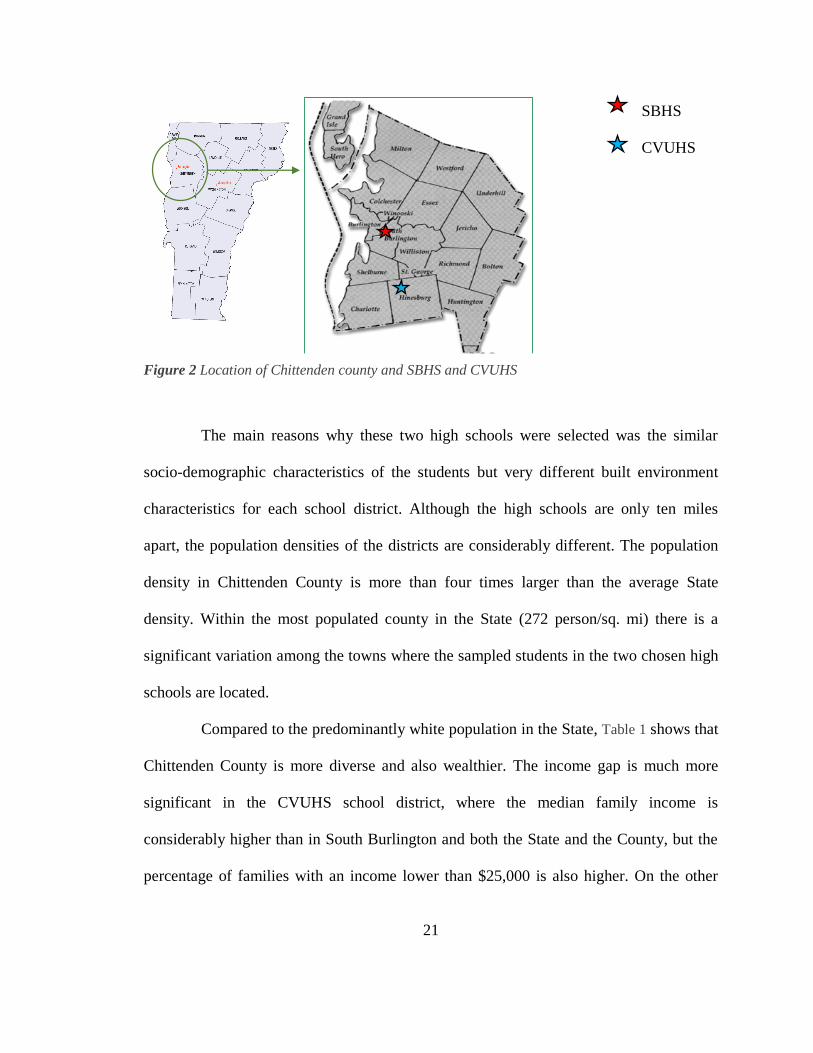
The two studied high schools are located in Chittenden County, the most

populated county in Vermont. Both selected High Schools are located in this County, and

20

therefore the survey results obtained are not representative of the rest of the State. Figure

1 and Figure 2 show the location of both high schools and the municipalities.

South Burlington High School (SBHS) is located in the town of South

Burlington. It has a population of 18,612 and a population density of 950 person/sq. mi

(3.5 times higher than the density in Chittenden County). Champlain Union Valley High

School (CVUHS) is located in the town of Hinesburg but the school district includes the

towns of Charlotte, Hinesburg, Shelburne, Williston, and St. George study there. The

total population of the five municipalities is 24,449, and the population density is 183

person/sq.mi (less than a half lower than in the County).

Figure 1 Location of the State of Vermont

21

The main reasons why these two high schools were selected was the similar

socio-demographic characteristics of the students but very different built environment

characteristics for each school district. Although the high schools are only ten miles

apart, the population densities of the districts are considerably different. The population

density in Chittenden County is more than four times larger than the average State

density. Within the most populated county in the State (272 person/sq. mi) there is a

significant variation among the towns where the sampled students in the two chosen high

schools are located.

Compared to the predominantly white population in the State, Table 1 shows that

Chittenden County is more diverse and also wealthier. The income gap is much more

significant in the CVUHS school district, where the median family income is

considerably higher than in South Burlington and both the State and the County, but the

percentage of families with an income lower than $25,000 is also higher. On the other

SBHS

CVUHS

Figure 2 Location of Chittenden county and SBHS and CVUHS

22

hand, very small differences can be seen when it comes to the percentage of workers

commuting by car in each town.

Table 1 Socio-demographic attributes of the two high school locations in Vermont

South

Burlington, VT

(South

Burlington

High School,

SBHS)

CVUHS High

School Town

District

Chittenden

County

Statewide

in VT

Median family income $83,000 $100,096 $84,284 $68,227

Families <$25,000 6.7% 19.5% 9.1% 12.6%

Families >$200k 8.3% 3.0% 8.3% 4.8%

% Workers commuting by car 86.7% 84.3% 80.9% 84.5%

% White only 90.6% 100.0% 94.2% 96.7%

% Hispanic (of any race) 1.0% 0.0% 1.0% 1.0%

% Asian (alone or with any

other race)

5.3% 0.0% 2.8% 1.0%

Source: U.S. Census Bureau, 2010

The survey questions included teenagers’ individual characteristics (age, gender,

race, bicycle ownership, driving license, mobile phone ownership), household (Lovejoy

and Handy 2013)characteristics (number of siblings, parent’s income, highest education

degree in household, number of vehicles in household), transportation related questions

(mode to/from school, use of technology for transportation) and also the address of the

household.

Study of Northern California

The study developed by UC Davis was an exploratory study that was designed

to identify key factors affecting whether or not high school students bicycle to school.

The survey was first designed and conducted in 2008 in Davis by Dr. Handy and her

research group. Davis is a prosperous university town with a population of around 65,000

23

located in Central Valley, California. Davis is well-known for its bicycling culture, but

not representative of Northern California Counties, which is why two more High Schools

were selected in which to conduct this survey, Tamalpais HS, in Marin County, and

Sequoia HS, in San Mateo County (Lovejoy and Handy 2013) (Figure 3).

Surveying Davis, Sequoia, and Tamalpais, the surveyed sample targets high

schools situated in more diverse built environments, enriching the mode choice

proportions. The two other schools included in the study meet this criterion in that they

are not nearly as bicycling-oriented as Davis, but are also in Northern California in

communities with at least some bicycling activity and infrastructure.

While a broader array of schools could better capture the full range of

experiences in different community types, Tamalpais and Sequoia together provide

diversity well beyond the Davis context. The three schools -- and the communities in

which they are situated – differ from each other in important ways, including the flavor

Davis HS

Tamalpais HS

Sequoia HS

Figure 3 Locations of Davis, Tamalpais, and Sequoia high schools in Northern California

24

and extent of bicycling culture in the broader community; the level of investment in

bicycling infrastructure in the vicinity of the school; the topography and catchment area

for the high school itself; and the socio-demographic make-up of each community.

In each case, researchers from California relied on a lead faculty member from

the school to help coordinate the distribution and collection of the surveys. These faculty

leads identified a date and time to conduct the survey that would work for their school’s

schedule, selecting a time period in which all students could be included while minimally

interfering with class time. During the designated time period, the teacher in each

classroom passed out the survey, read a statement assuring students that it was voluntary,

and then collected the completed surveys. Although cooperation was invited via

encouragement from the lead faculty person, as well as endorsed by school

administration, teachers in each classroom were not required to participate in the study.

The total sample size of this data set is 2,900; 1164 students from Davis, 1011

from Sequoia, and 725 from Tamalpais High School.

Specific questions asked in the survey can be found in Appendix B. In the

survey transportation-related, socio demographic questions, and technology use questions

were asked. In addition to transportation behavior related questions, attitudinal questions

were also answered by the students in a scale of 1 to 5. These questions revealed

teenagers’ perspective and tendency of more general matters, such as the environment.

Including these attitudinal questions complemented more direct questions such as the

mode choice, and better frame teenagers’ behavior. Although exact household location

25

was not asked, respondents provided the closest street intersection in order to

geographically locate it for further analysis.

With respect to demographics, all three communities are somewhat wealthier

than the state as a whole, according to the 2010 Census (see Table 2). Mill Valley (served

by Tamalpais High) is especially wealthy and white. The community served by Sequoia

is more economically and racially diverse than Davis or Tamalpais, and importantly

includes students from areas beyond Redwood City where the school itself is located (and

for which statistics are shown in Table 2).

Table 2 Socio-demographic attributes of the three high school locations in California

Davis, CA

(Davis

High)

Redwood

City, CA

(Sequoia

High)

Mill Valley,

CA

(Tamalpais

High)

Statewide

in CA

Median family income $106,586 $88,525 $167,561 $70,231

Families <$25,000 11.9% 9.5% 2.9% 15.2%

Families $200k+ 16.6% 17.3% 40.1% 8.4%

% workers commuting by car 68.9% 90.3% 80.1% 89.3%

% white (only) 64.9% 60.2% 88.8% 57.6%

% Hispanic (of any race) 12.5% 38.8% 4.5% 37.6%

% Asian (alone or with any other

race)

25.3% 13.1% 7.7% 14.9%

Source: U.S. Census Bureau, 2010

GEOGRAPHIC DATA

Besides household location (addresses for the Vermont schools and closest

intersections for the California ones), additional geographical information is considered

in the analysis with various built environment variables. The distance from home to high

schools can be directly calculated from the survey, but little more is known about the

neighborhoods in which the households are located. In order to analyze the built

26

environment, the following variables are considered: centrality, job access, neighborhood

income, general population density and population density of teenagers.

Centrality represents the distance from each household to the closest urban area.

The definition of “urban area” used in this study is the one from the Census: 50,000 or

more people. Common central place models of urban form hold that properties closer to

the center of a region have higher accessibility to the rich and dense work and

consumption opportunities that tend to be located in the center (Cortright 2009).

For job access, data drawn from the Census Bureau’s Zip Code Business

Patterns database is used. Zip code information is assigned to each household and, in

addition, the number of jobs within 1 mile (walking), 5 miles (biking) and 10 miles of the

households are computed. This measure of job accessibility aims at capturing activity

options for each household related to their locations, which are likely to increase relative

to the proximity to employment opportunities.

Neighborhood income is determined as the Census 2010’s reported values for

median household income of the census block group in which each household is located.

These income levels can be used as proxies for neighborhood quality and to reflect the

external effects associated with the income level of one’s neighbors. Neighborhood

income levels are frequently associated with crime rates and school quality (Cortright

2009). Although these are not factors directly studied in this analysis, neighborhood

income levels have shown to have impacts on the activity levels of people (Fischer, Li et

al. 2004) and can, therefore, have significant effects in teenagers’ mode choice and

technology use for transportation.

27

In addition, population density in neighborhoods have shown to affect travel

behavior and activity levels of teenagers (Newacheck, Hung et al. 2003, McDonald 2008,

Saelens and Handy 2008, Brownson, Hoehner et al. 2009, Bungum, Lounsbery et al.

2009). Analyzing the density of teenagers living around each of the studied households

will allow us to better define the characteristics of the built environment. This analysis is

developed using Census 2010 population data, and looking at the number of young

people living within 1 mile, 5 miles, and 10 miles from the homes. All the geographical

data has been obtained through ESRI.

DESCRIPTIVE STATISTICS

The sample sizes for each high school are considerably different. The total

number of students who answered the survey in South Burlington and Champlain Valley

are 146, whereas in Davis, Sequoia and Tamalpais, this number is much larger (Table 3).

While the Vermont survey has fewer respondents, it is also a richer set of data with more

in-depth questions and complementary qualitative data.

Analyzing the percentage of students accessing their respective high schools in

any kind of active transportation mode (walk, bike, skateboard), it can be seen that, not

surprisingly, Davis has the highest proportion. Due to its geographical characteristics as

well as biking habits and infrastructure, the number of students biking to high school can

be up to six times higher than in Tamalpais or Sequoia (Table 3).

28

Table 3 Mode choice proportion per high school

Davis Sequoia Tamalpais SBHS CVUHS

Bike/skate 33.8% 5.6% 6.6% 0.8% 0.6%

Walk 5.8% 30.6% 22.1% 8.5% 1.5%

Car/motorcycle 61.2% 70.7% 77.5% 50.2% 55.1%

Bus/train 6.7% 9.2% 9.5% 40.5% 42.8%

Total 1164 1011 725 84 61

Since the descriptive statistics show many similarities among all sampled

populations, data from the five high schools has been combined for mode choice

distribution analysis. The following figures show the distribution of mode choices among

teenagers by high school, age and gender.

Figures 1 through 4 show the mode choice distribution by grade and Figures 5

through 8 the mode distribution by gender.

Figure 4 Mode choice by grade in South Burlington High School

0.00%

10.00%

20.00%

30.00%

40.00%

50.00%

60.00%

70.00%

80.00%

90.00%

100.00%

9 10 11 12

Mo

de

dis

trib

uti

on

Grades

Mode choice by grade SBHS

Bycicle Bus Drive Ride Walk

29

Figure 5 Mode choice by grade in Champlain Valley Union High School

Figure 6 Mode choice by grade in Davis High School

0.00%

10.00%

20.00%

30.00%

40.00%

50.00%

60.00%

70.00%

80.00%

90.00%

100.00%

9 10 11 12

Mode

dis

trib

uti

on

Grade

Mode choice by grade CVUHS

Bike Walk Ride Drive Bus

0.00%

10.00%

20.00%

30.00%

40.00%

50.00%

60.00%

70.00%

80.00%

90.00%

100.00%

10 11 12

Mode

dis

trib

uti

on

Grade

Mode choice by grade DAVIS

Bicycle Walk Ride Drive Bus

30

Figure 7 Mode choice by grade in Tamalpais High School

Figure 6 Mode choice by grade in Sequoia High School

0.00%

10.00%

20.00%

30.00%

40.00%

50.00%

60.00%

70.00%

80.00%

90.00%

100.00%

9 10 11 12

Mode

dis

trib

uti

on

Grade

Mode choice by grade TAMALPAIS


0.00%

10.00%

20.00%

30.00%

40.00%

50.00%

60.00%

70.00%

80.00%

90.00%

100.00%

9 10 11 12

Mode

dis

trib

uti

on

Grade

Mode choice by grade SEQUOIA


31

Figure 7 Mode choice by gender South Burlington High School

Figure 8 Mode choice by gender Champlain Valley Union High School

0.00% 4.51% 34.18% 31.28% 30.03%

1.71% 12.21% 21.38% 17.48% 47.22%

0%

10%

20%

30%

40%

50%

60%

70%

80%

90%

100%


Gen

der

dis

trib

uti

on

Mode

Mode choice by gender SBHS

Female Male

0.00% 4.12% 38.23% 26.59% 31.06%

1.12% 9.30% 16.08% 20.95% 52.55%

0%

10%

20%

30%

40%

50%

60%

70%

80%

90%

100%


Gen

der

dit

rib

uti

on

Mode

Mode choice by gender CVUHS

Female Male

32

Figure 9 Mode choice by gender DAVIS

Figure 10 Mode choice by gender TAMALPAIS

26.52% 5.55% 33.97% 29.12% 4.85%

40.70% 3.13% 25.41% 28.36% 2.39%

0%

10%

20%

30%

40%

50%

60%

70%

80%

90%

100%


Gen

der

dis

trib

uti

on

Mode

Mode distribution by gender, DAVIS

Female Male

2.58% 13.47% 51.29% 27.79% 4.87%

10.59% 14.71% 41.76% 26.18% 6.76%

0%

10%

20%

30%

40%

50%

60%

70%

80%

90%

100%


Gen

der

dis

trib

uti

on

Mode

Mode choice by Gender TAMALPAIS

Female Male

33

Figure 11 Mode choice by gender SEQUOIA

Although the respondents of the surveys were students from different counties

and states, when looking at the effect of gender and age on their travel behavior, we can

see that students of all schools follow a similar pattern. The proportion of students who

drive to school increases for older teenagers. In fact, carpooling or riding with others

follows the opposite trend as driving their own car, and this can be seen in all surveyed

high schools. Although biking rates in Davis High School are much higher than in the

other schools, the proportions of students walking, biking and riding the bus to school

also decreases with age, as with all surveyed high schools. Regarding gender the

distribution in teenagers’ mode choice, it can also be seen that very similar patterns occur

in every surveyed high school. Males walk and bike more, and ride with others less than

2.37% 20.16% 56.92% 15.02% 5.53%

8.11% 21.17% 48.65% 16.67% 5.41%

0%

10%

20%

30%

40%

50%

60%

70%

80%

90%

100%


Gen

der

dis

trib

uti

on

Mode

Mode choice by Gender SEQUOIA

Female Male

34

females. They also tend to take the bus more, and overall choose to use the car less than

females to access high school.

DATA PROCESSING

As previously stated, data used for this study has two main sources. One, survey

data (developed and conducted by researchers in UVM and UCDavis), and the other,

geographical data. In order to link both datasets together, the data were carefully

processed.

For both Vermont and Californian surveys, household location information was

asked of each student. This information consisted of exact home address (for Vermont)

and closest street intersection (for California). These point data were geocoded in order to

calculate travel distances to school as well as built environment characteristics. Some of

these data, however, were either missing or were not recognized as valid locations (Table

4). Since distance to school is a key variable, only those records with valid values were

selected for analysis.

Table 4 Geocoding percentages and matches per high school

High

School

N total N

geocoded

Geocoded

%

Missing cross-

streets /

address (%)

Not located

(%)

Davis 1164 859 73.8 20 6.2

Sequoia 1011 652 64.5 19.9 15.6

Tamalpais 725 492 67.9 18.3 13.8

SBHS 62 57 91.9 4.1 4.0

CVUHS 83 75 90.4 4.5 5.1

One-mile, five-mile, and ten-mile service areas were calculated around each

surveyed household, and these polygons were used to clip census tract data as well as

35

street network data in order to calculate population parameters and network availability

for each teenager. One-mile service areas represent walking distance, five-mile biking

distance and ten-mile driving distance. Similarly, each household was spatially joined to

geographical Federal Information Processing Standards (FIPS), and urban areas and

cluster polygons.

Data analysis

Most of the variables used in the study were categorical. The surveys provided

multiple options to choose from for many questions, but for the purpose of this analysis,

such results have been recoded, grouped and simplified. The following table shows the

answer options of the questions used in this study, and the variable recoding.

Most of the variables were recoded as binary. When developing the models,

having variables with multiple categories would give unstable results due to the small

number of records per category. Except for the variable “grade”, which was kept as four

categories, the rest of the categorical variables were reduced to only two categories.

Mode to school variable, as the outcome variable in the developed model, was simplified

in four categories: walk/bike, bus or other, ride, and drive. Similarly, in order to model

the frequency of technology use for transportation, this variable was also simplified from

five to three, but still ordinal, categories. Other variables that became significant or

increased influence in the output when recoding them were: having or not having a

cellphone, having or not a driving license, parent’s education, and number of siblings in

the family. Table 5 shows the summary of the data processing for recoding each variable.

36

Table 5 Survey variables recoding

SURVEY QUESTION Variable Alternatives Recoding

What grade are you in? Grade 9,10,11,12

What is your gender? Gender Male, Female

How do you usually get

to school?

Mode to

school

I bicycle

I walk

I skateboard

A friend drives me

A family member drives me

Another parent drives me

I drive myself

I take the bus

Other

Bike/Walk

Bike/Walk

Bus or other

Ride

Ride

Ride

Drive

Bus or other

Bus or other

Do you currently own or

have regular access to a

functioning bicycle?

Bicycle No

Yes

Do you have a

cellphone?

Cell phone No

Yes [not a smartphone (SP)]

Yes, a smartphone

Not a SP

Not a SP

A SP

How often do you use a

cell phone or technology

to arrange

transportation?

Frequency of

technology

use for

transportation

Every day

Most days of the week

A few days a week

Once a week or less

Never

High

Medium

Medium

Low

Low

Most recent driver’s

license/permit

License Provisional license

Regular driver’s license

Driver learner’s permit

I do not have a license

Yes

Yes

No

No

Parent’s education Education Some High School

High School

Some College

Associate Degree

Bachelor Degree

Advanced Degree

Other

Low

Low

Low

High

High

High

Low

Do you have siblings

currently living with

you?

Siblings No

Yes, older

Yes, younger

The following figures show the distribution for each variable, and the recoding approach

chosen to analyze and model the data. Values are shown as % of the total N value

(N=1780).

37

Figure 12 Bicycle Distribution

Figure 13 Phone Distribution

20.18

79.82

0.00 10.00 20.00 30.00 40.00 50.00 60.00 70.00 80.00 90.00

No

Yes

%

22.32

4.05

73.64

0.00 20.00 40.00 60.00 80.00

Dumb

No

Smart

%

Typ

e o

f P

ho

ne

26.36

73.64

0.00 20.00 40.00 60.00 80.00

Not Smart

Smart

%

38

Figure 14 Technology Use Distribution

Figure 15 Driving License Distribution

0 10 20 30 40 50 60 70

Yes

No

%

138

368

370

335

677

0 200 400 600 800

Never

Once a week or less

A few days a week

Most days of week

Everyday

506

705

677

0 200 400 600 800

Low

Medium

High

39

Figure 16 Education Distribution

Figure 17 Siblings Distribution

3.32

6.91

10.01

2.92

25.80

40.53

10.51

0.00 20.00 40.00 60.00

Some HS

HS

Some College

Associate Degree

Bachelor Degree

Advanced Degree

Other

%

Edu

cati

on

30.75

69.25

0.00 20.00 40.00 60.00 80.00

Low

High

%

30.86

19.11

50.03

0.00 20.00 40.00 60.00

No

Older

Younger

%

30.86

69.14

0.00 20.00 40.00 60.00 80.00

No

Yes

%

40

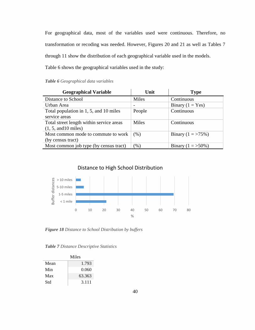
For geographical data, most of the variables used were continuous. Therefore, no

transformation or recoding was needed. However, Figures 20 and 21 as well as Tables 7

through 11 show the distribution of each geographical variable used in the models.

Table 6 shows the geographical variables used in the study:

Table 6 Geographical data variables

Geographical Variable Unit Type

Distance to School Miles Continuous

Urban Area - Binary (1 = Yes)

Total population in 1, 5, and 10 miles

service areas

People Continuous

Total street length within service areas

(1, 5, and10 miles)

Miles Continuous

Most common mode to commute to work

(by census tract)

(%) Binary (1 = >75%)

Most common job type (by census tract) (%) Binary (1 = >50%)

Table 7 Distance Descriptive Statistics

Miles

Mean 1.793

Min 0.060

Max 63.363

Std 3.111

0 10 20 30 40 50 60 70 80

< 1 mile

1-5 miles

5-10 miles

> 10 miles

%

Bu

ffer

dis

tan

ces

Distance to High School Distribution

Figure 18 Distance to School Distribution by buffers

41

Table 8 Population density (total and teenager) by distance buffers. Descriptive Statistics.

Tot. Pop 1

mile

Tot. Pop 5

miles

Tot. Pop 10

mile

Teen Pop. 1

mile

Teen Pop. 5

miles

Teen Pop.

10 miles

Mean 6755.842 440021.484 388186.248 380.993 6363.229 6695.615

Min 265.746 0.000 35621.647 0.218 0.000 44.711

Max 15066.000 334361.113 904421.120 2167.258 25526.563 37095.482

Std 2492.076 50210.093 184376.263 519.861 3060.569 6175.335

Table 9 Street length descriptive statistics by distance buffers

Street Length1 mile Street Length 5 miles Street Length 10 miles

Mean 0.454 5.765 9.278

Min 0.040 0.303 0.668

Max 1.037 16.066 31.299

Std 0.202 2.686 5.536

Table 10 Distribution of transportation mode for daily commute by census tract (%)

DriveAlone Carpool PublicTransp Walk MotoBikeEtc WorkHome

Mean 63.447 7.543 6.859 3.165 9.579 7.504

Min 20.505 1.280 0.000 0.000 0.000 0.000

Max 91.943 26.576 16.387 18.707 49.647 21.204

Std 10.788 4.082 3.973 2.697 10.295 3.954

Table 11 Distribution of Occupations by census tract (%)

Management ServiceProp Sales Natura Production Military

Mean 53.702 11.505 18.943 4.521 4.766 0.053

Min 9.329 1.749 7.899 0.000 0.436 0.000

Max 80.739 52.478 34.846 34.981 21.237 1.653

Std 16.307 8.889 5.555 4.007 3.929 0.250

42

Table 12 Attitudinal questions included in the models

Attitudinal variable Question # Categorical scale

I like bicycling C 1 (Strongly disagree) – 5 (Strongly Agree)

Bicycling is my usual way

of getting around town

F 1 (Strongly disagree) – 5 (Strongly Agree)

I like being driven places G 1 (Strongly disagree) – 5 (Strongly Agree)

My parents encourage me to

bicycle

H 1 (Strongly disagree) – 5 (Strongly Agree)

I feel comfortable getting

places on my own

J 1 (Strongly disagree) – 5 (Strongly Agree)

I like riding the bus L 1 (Strongly disagree) – 5 (Strongly Agree)

I can rely on my parents to

drive me places

N 1 (Strongly disagree) – 5 (Strongly Agree)

I need a car to do the things

I like to do

O 1 (Strongly disagree) – 5 (Strongly Agree)

One or both my parents

bicycle frequently

S 1 (Strongly disagree) – 5 (Strongly Agree)

I have lots of stuff to carry

to school

W 1 (Strongly disagree) – 5 (Strongly Agree)

I live too far away from

school to bicycle there

BB 1 (Strongly disagree) – 5 (Strongly Agree)

0

200

400

600

800

1000

1200

1400

1600

1800

2000

C F G H J L N O S W BB

Nu

mb

er o

f te

ens

Attitude question

Attitudinal varibales frequencies

1 2 3 4 5

43

CHAPTER 4 – MODE CHOICE TO AND FROM SCHOOL

STATISTICAL METHOD

All variables in the survey data set were binary or categorical variables. Since

this research aimed to determine the influence of different factors on the mode choice to

and from school, the outcome variables used in the models were the mode choice to and

from school. Since mode choice for each surveyed teenager is a multinomial variable,

multinomial logistic regression models were used.

The multinomial logistic regression function is shown in equation 3-1 (Agresti

2007). Here, the parameter α is the intercept term and βn determines the rate of increase or

decrease of the variable xn.

Equation 4-1 – Logistic Regression Function

ln(𝜋(𝑥)

1 − 𝜋(𝑥)) = 𝛼 + 𝛽1𝑥1 + 𝛽2𝑥2 +…+ 𝛽𝑛𝑥𝑛

The odds ratio is a statistical outcome that describes the strength of association

between two variables. Here, the odds ratios between the mode choice and predictor

variables are calculated. Odds ratios and their confidence intervals can be obtained from

the parameter 𝛽 from the logistic regression, and are shown in Equation 3-2 (Agresti

2007).

Equation 4-2 – Odds Ratio and Confidence Interval

Odds Ratio = 𝑒𝛽

Confidence Interval = (𝑒𝛽±𝑧𝛼2(𝑆𝐸))

Odds ratios equal to 1.0 indicate that the event or condition is equally likely to

happen for either levels of the variable. Ratios larger than 1.0 indicate an increased odds

44

for the event in the first group. On the other hand, odds ratios less than 1.0 mean that the

reverse is true but it can be difficult to interpret (for example an odds ratio of 0.75 would

mean that the outcome is 25% less likely for one group). Instead, calculating the inverse

of the odds ratio can lead to a more meaningful and intuitive understanding. The

confidence interval describes the margin of error to be expected from the dataset. If this

interval includes 1.0, there is not enough evidence to conclude an increased odds for one

level of the variable or the other (Agresti 2007).

The odds ratios were calculated to test whether various factors were more

strongly associated with one mode versus another. In particular, it was used to test

whether teenagers’ choice of biking, walking, riding the bus, or riding with someone had

increased odds compared to driving alone to school.

MODELING MODE CHOICE

Regression models can be used to serve various research needs. In this case, the

multinomial logistic regressions were used in order to develop models that allowed

interactions between the variables tested to see if they are significant factors in mode

choice to and from school. Odds ratios were calculated from the multinomial logistic

regressions. These regressions were not developed as predictive mode choice models. As

seen by the R2 in Tables 7-9, the fits for the models are not very high. The R2 value

describes how well the data fit the model by calculating the error variance. JMP

calculates the R2 by taking the ratio of the difference between the reduced (only intercept)

and full (one with all variables) models’ negative log-likelihoods (SAS 2012). Values

close to 1.0 indicate the model fits the data well for the purposes of prediction of future

outcomes. Generally, incorporating more variables into the model can produce higher R2

45

values, but these additional variables might not be available, or may become very

complex. Besides, nominal models rarely have high R2 values (SAS 2012).

The logistic regression results are shown in the next section, as well as the

discussion.

RESULTS AND DISCUSSION

None of the explanatory variables were alternative specific, therefore each was

entered into the model as three separate interactions with the three non-reference

alternatives. For this section of the study, three different models have been developed. In

order to answer the research questions listed in the beginning of this document, one

model (Model 4.1) considered the effects of various socio demographic, built

environment and virtual environment variables in the mode choice of all surveyed

teenagers in the five high schools (Table 13). Then, the effect of the attitude of teenagers

is analyzed using additional attitudinal data from the California surveys. For this analysis,

first, a model containing the same variables as in Model 4.1 has been run but only for the

three high schools in California (Table 14). And then, attitudinal variables have been

added to such model in order to determine the effects of such variables in the outcome

(Table 15). Having both models allows for comparisons of the pseudo R square values

and determine the effectiveness of considering attitudinal factors in these type of

behavioral studies.

46

Model 4.1: Combined California and Vermont High Schools Model

The results for Model 4.1 – corresponding to the question of “What socio-

demographic and built environment factors are relevant for students from both states?” -

are shown in Table 13. It includes explanatory variables from all three categories (socio-

demographic, built environment, and virtual environment) and has an entropy r-square of

0.3996. Table 13 shows that each explanatory variable in the multinomial logit model has

at least one statistically significant interaction with the alternatives to at least 95%

confidence, and they all have the expected signs.

Table 13 Mode to school Nominal Logistic Regression model results (Five high schools)

VARIABLE Estimate Standard

error

ChiSquare

Bike or Walk vs. Drive to School

Intercept -1.557 0.520 8.96

Grade (9 vs. 12) -0.065 0.365 0.03

Grade (10 vs. 12) 0.218 0.195 1.25

Grade (11 vs. 12) -0.151 0.180 0.70

Gender (male vs. female) 0.169 0.086 3.84

Bike (yes vs. no) 0.495 0.123 8.592

Parents education (High vs. low) 0.087 0.113 0.59

Driving license (yes vs. no) -2.302 0.149 236.27

Frequency of technology use (high vs. low) -0.378 0.089 17.74

Phone (smartphone vs. not a smartphone) 0.341 0.103 11.04

Distance to high school (miles) -0.866 0.099 93.05

Population within 1 mile service area -1.04 e-04 5.64 e-05 3.42

Population within 5 miles service area 5.07 e-06 2.48 e-06 4.20

Teenager population within 1 mile service

area

4.87 e-04 2.35 e-04 4.28

Teenager population within 5 miles service

area

1.59 e-04 5.09 e-05 9.82

Total street length within 1 mile service

area

2.808 0.993 7.99

Total street length within 5 mile service area -0.025 0.068 0.13

47

General trend of driving to commute to

work in the census tract (Over 75% vs. less

than 75%)

-0.636 0.124 26.37

Maximum of the census tract pop. works in

management positions

0.828 0.16 26.75

Bus vs. Drive to School

Intercept 0.326 0.661 0.24

Grade (9 vs. 12) 0.326 0.403 0.66

Grade (10 vs. 12) 0.089 0.256 0.12

Grade (11 vs. 12) 0.138 0.252 0.30


Bike (No vs. yes) 0.186 0.187 0.95

Parents education (High vs. low) -0.558 0.165 11.37


Frequency of technology use (low vs. high) 0.204 0.141 2.11


Distance to high school (miles) 0.066 0.033 3.80

Population within 1 mile service area 6.608 e-05 7.36 e-05 0.81


Teenager population within 1 mile service area -2.04 e-05 4.90 e-04 0.00


area

9.453 e-05 8.21 e-05 1.21


area

-3.702 1.348 7.54


area

-0.206 0.0972 4.50

General trend of driving to commute to work

in the census tract (Over 75% vs. less than 75%)

0.213 0.174 1.50



0.017 0.193 0.01

Ride with someone vs. Drive to School

Intercept 0.085 0.478 0.03

Grade (9 vs. 12) 0.299 0.347 0.75

Grade (10 vs. 12) 0.177 0.189 0.87

Grade (11 vs. 12) -0.032 0.175 0.03

Gender (male vs. female) -0.125 0.087 2.06

Bike (No vs. yes) 0.152 0.112 1.03


48

Driving license (yes vs. no) 2.557 0.145 311.04

Frequency of technology use (low vs. high) -0.043 0.089 0.23


Distance to high school (miles) -3.52 e-04 4.89 e-05 0.45

Population within 1 mile service area 6.58 e-05 5.43 e-06 1.47

Population within 5 miles service area -5.24 e-07 2.35 e-06 0.05

Teenager population within 1 mile service area -3.11 e-04 2.64 e-04 1.38


area

2.55 e-06 4.71 e-05 0.00


Total street length within 5 mile service area 0.169 0.065 6.75



-0.122 0.114 1.13



0.439 0.148 8.76

Entropy R square 0.3996

Note: Values in bold show a significance of 0.05 p-values or lower.

Regarding the comparison between choosing biking or walking, or driving to

school, more variables are significant than for other mode choice comparisons. Those

students who own or have access to a functioning bicycle, do not have a driving license

or do not frequently use technology for arranging transportation may positively affect

their likelihood to choose active transportation modes to access school. Although in this

particular case, the education of the parents did not show any significance, these variables

could be indirectly related to the income of the family and, therefore, with the potential

available mode choice alternatives for each teenager. If the majority of the workers in the

census tract where the teenagers’ households were located worked in management

positions (i.e., business, financial, computer, engineering, science, legal, education, and

media occupations), teenagers seem to more likely bike or walk to school. Looking at

built environment variables, distance to school has a very significant effect on the choice

49

of active transportation modes among the studied teenagers. The larger the distance they

have to travel, the less likely it is for them to walk or bike to school. Similarly, teenagers

living in more populated areas, both within the one- or five-mile service area buffers,

may be more likely to walk or bike to school. Street density also showed a potential

positive correlation with the use of active transportation modes versus driving to school

among teenagers.

Interpreting the results comparing bus or driving as the mode choice to access

high school, fewer variables were significant in the model. The population density in the

area did not impact their mode choice, but income related variables were significant. Not

having a bicycle, living in a less educated household, and not having a driving license

may increase the likelihood of teenagers riding the bus versus driving to school. Also, a

more frequent use of technologies for arranging transportation shows an increase

tendency on the use of buses for accessing school. On the other hand, better street

connectivity within one mile and five mile buffers from the teenagers’ households

showed a negative effect on bus ridership among the studied teenagers’ mode choice to

school. As it has been previously mentioned, these models do not show causality, but

association. In fact, we can see that having a smartphone may increase the likelihood of

teenagers to take the bus vs. drive to school. However, one could argue that since a

teenagers has the need or depends on public transportation to move around has a higher

need of owning a smartphone. There is definitely an association between these two

variables, the data used for this particular analysis is simply not detailed enough to

determine the exact direction of such association.

50

When looking at the results for getting a ride from someone else versus driving

themselves to school, only two variables were significant. Having a driving license has a

very strong impact on choosing to ride or drive to school among the studied teenagers.

Not having a driving license considerably increases the likelihood of teens to ride with

others. Similar to the income related variables mentioned in the other model sections,

those teenagers living in census tracts where workers had management occupations were

also more likely to take rides to school rather than drive themselves.

Model 4.2: California High Schools Model


demographic and built environment factors are relevant for students from California?” -

are shown in Table 14. It includes explanatory variables from all three categories (socio-

demographic, built environment, and virtual environment) and has an entropy r-square of

0.4074. Table 14 shows that each explanatory variable in the multinomial logit model has

at least one statistically significant interaction with the alternatives to at least 95%

confidence, and they all have the expected signs. This model only includes records from

CA high schools in order to compare the results to the following model (4-3) which

includes attitudinal variables (only available in the CA survey).

The same variables as in Model 4.1 were included to build the models. Although

the significance of such variables is not exactly the same, it is very similar.

51

Table 14 Mode to school Nominal Logistic Regression model results (California high schools)


error

ChiSquare


Intercept 3.103 0.645 23.14

Grade (9 vs. 12) -0.301 0.370 0.66

Grade (10 vs. 12) 0.368 0.201 3.34

Grade (11 vs. 12) -0.139 0.184 0.57


Bike (yes vs. no) 0.395 0.135 8.53



Frequency of technology use (high vs. low) -0.417 0.095 19.43

Phone (smartphone vs. not a smartphone) -0.316 0.109 8.34


Population within 1 mile service area 0.0001 5.94e-05 2.83



area

0.00011 0.00025 4.88


area

0.00016 5.096e-05 9.82



area

0.344 0.086 16.00



-0.216 0.170 1.62



0.756 0.153 25.46


Intercept -0.545 0.799 0.46

Grade (9 vs. 12) 0.034 0.444 0.01

Grade (10 vs. 12) 0.264 0.285 0.86

Grade (11 vs. 12) 0.032 0.287 0.01


Bike (No vs. yes) 0.184 0.189 0.95


52





Population within 1 mile service area -8.37e-05 0.00009 0.94


Teenager population within 1 mile service area 3.88 e-04 5.37 e-04 0.52


area

9.71e-05 8.36e-05 1.35





-0.069 0.226 0.1



0.023 0.187 0.02


Intercept 0.310 0.530 0.34

Grade (9 vs. 12) 0.116 0.353 0.11

Grade (10 vs. 12) 0.314 0.194 2.61

Grade (11 vs. 12) -0.065 0.178 0.13


Bike (No vs. yes) -0.238 0.127 3.54






Population within 1 mile service area 3.42e-05 5.25e-05 0.42

Population within 5 miles service area -5.12 e-07 2.31 e-06 0.06

Teenager population within 1 mile service area -0.0005 0.0003 2.72


area

2.552 0.000048 0.00





-0.223 0.149 2.24



0.439 0.148 8.76

53



Regarding the comparison between choosing biking or walking, or driving to

school, more variables are significant than for other mode choice comparisons. Males are

more likely to choose active transportation modes to access high school than females.

Those students who own or have access to a functioning bicycle, do not have a driving

license or do not frequently use technology for arranging transportation show a higher

likelihood to choose active transportation modes to access high school. If the majority of

the workers in the census tract where the teenagers’ household was located worked in

management positions (business, financial, computer, engineering, science, legal,

education, and media occupations), the results show that teenagers may be more likely to

bike or walk to school.

Comparing to Model 4.1 biking/walking vs. driving results, having higher

population densities are significant in under 1 mile distances and not under 5 miles, and

gender also became significant. In fact, when analyzing California teenagers exclusively,

men are more likely to bike/walk to school than women. Distance to school is significant

when analyzing bus vs. drive modes among teenagers in California, however, other built

environment variables such as street connectivity did not show any significance in this

model, unlike in Model 4.1.

Model 4.3: California High Schools Model with attitudinal variables

The results for model 4.3 – corresponding to the question of “What attitudinal

factors influence the California teenagers? - are shown in Table 15. It includes

54

explanatory variables from all three categories (socio-demographic, built environment,

and virtual environment) and also attitude variables from the California survey. The

entropy r-square of 0.5840 is considerably higher than the one on model 4.2, which

means that including such variables increases the accuracy of the model and better

explains the studied population. The significance of the variables that were also included

in model 4.2 may have varied in model 4.3. All new variables included in this model

(attitudinal) have at least one statistically significant interaction with the alternatives to at

least 95% confidence, and they all have the expected signs.

Table 15 Mode to school Nominal Logistic Regression model results, plus attitudinal factors

(California high schools)


error

ChiSquare


Intercept -1.467 2.007 0.53

Grade (9 vs. 12) -1.578 0.495 10.17

Grade (10 vs. 12) 0.564 0.279 4.06

Grade (11 vs. 12) 0.248 0.261 0.91


Bike (No vs. yes) 0.055 0.201 0.08






Population within 1 mile service area -1.95 e-04 8.65e-5 5.09

Population within 5 miles service area 1.92e-5 5.78e-6 10.99


area

8.17 e-04 3.59 e-04 5.18


area

7.07e-5 1.53 e-04 0.21


55



in the census tract (Over 75% vs. less than

75%)

-0.330 0.227 2.13



0.274 0.24 1.22

I like bicycling 0.394 0.146 7.3

Bicycling is my usual way of getting

around town

1.463 0.170 73.95

I like being driven places 0.262 0.143 3.37

My parents/guardians encourage me to

bicycle

0.548 0.144 14.44

I feel comfortable getting places on my

own

0.459 0.171 7.22

I like riding the bus 0.227 0.126 3.28

I can rely on my parents/guardians to drive

me places

-0.120 0.125 0.92

I need a car to do the things I like to do -0.359 0.127 7.91

One or both of my parents/guardians

bicycle frequently

0.459 0.109 17.83

I have lots of stuff to carry to school -0.632 0.125 25.59

I live too far away from school to bicycle

there

-0.765 0.147 27.13


Intercept -15.508 121306.79 0.00

Grade (9 vs. 12) -0.128 0.588 0.05

Grade (10 vs. 12) 0.333 0.384 0.75

Grade (11 vs. 12) 0.358 0.391 0.84


Bike (No vs. yes) -0.105 0.272 0.15






Population within 1 mile service area -6.32e-5 1.31 e-04 0.23

Population within 5 miles service area 6.60e-6 6.49e-6 1.04


area

3.77 e-04 7.46 e-05 0.26

56


area

3.09 e-04 1.52 e-04 4.16





75%)

-0.131 0.337 0.15



0.185 0.381 0.24

I like bicycling 0.081 0.209 0.15

Bicycling is my usual way of getting around

town

0.438 0.244 3.22



bicycle

0.218 0.230 0.90


own

-0.642 0.229 7.88



me places

-0.324 0.202 2.56


One or both of my parents/guardians bicycle

frequently

-0.195 0.187 1.09



there

0.219 0.168 1.70


Intercept 0.249 1.611 0.02

Grade (9 vs. 12) -0.538 0.410 1.72

Grade (10 vs. 12) 0.392 0.247 2.51

Grade (11 vs. 12) 0.102 0.231 0.20


Bike (No vs. yes) -0.413 0.176 5.50






Population within 1 mile service area 6.08e-5 7.38e-5 0.68

57

Population within 5 miles service area 4.41 e-06 4.26e-6 1.07


area

2.59 e-04 3.55 e-05 0.54


area

1.93 e-04 1.06 e-04 3.34





75%)

0.087 0.195 0.20

Maximum of the census tract pop. works

in management positions

0.427 0.204 4.38

I like bicycling -0.109 0.130 0.70

Bicycling is my usual way of getting

around town

0.407 0.156 6.83



bicycle

0.203 0.129 2.45


own

-0.689 0.143 23.29



me places

0.064 0.116 0.31


One or both of my parents/guardians

bicycle frequently

-0.258 0.100 6.63



there

0.124 0.100 1.53



Attitudinal factors have shown to clearly increase the R square value of the

model. When it comes to biking or walking versus driving, teenagers’ personal opinion

about biking has a very strong effect on their mode choice to school. Logically, strongly

agreeing with the statement of “Bicycling is my usual way of getting around places” has

58

the most positive effect on likelihood of choosing biking/walking as the transportation

mode to school among California teenagers. The fact that they like bicycling as in the “I

like bicycling” statement also shows a positive effect on the likelihood of the teenager

biking to school. Similarly, if their parents either encourage them to bike or even they

bicycle frequently themselves, also may increase their likelihood to bike to school. Note

that the association between liking a specific mode, such as bicycling or riding the bus,

and the use of that mode may be bidirectional. A teenager liking to ride the bus may

increase his or her likelihood to choose the bus to go to school. On the other hand if a

teenager’s only mode of transportation to school is the bus, he or she may also be likely

to enjoy more such mode. This study does not analyze each variable deep enough, and

therefore the causality between the actions cannot be determined. Although the model

does show association, and therefore we can state that such variables have effect on

eachother.

Signs of teenagers’ independence, as in “I feel comfortable getting places on my

own” has also the same effect on the studied outcome. On the other hand, those teenagers

who need a car to do the things they like to do, have lots of stuff to carry to school, or

agree with the statement that “They live too far away from school to bicycle there” are

less likely choose to bike or walk to school.

Teenagers’ independence has the opposite effect on their likelihood of riding the

bus versus driving to school. Those who strongly agree with the statement of “I feel

comfortable getting places on my own” are more likely to drive to school than to ride the

bus. Having to carry heavy stuff to school, as for the Bike/Walk versus Drive model

59

results also has a negative effect on choosing taking the bus among the surveyed

teenagers. The only attitudinal variable with a positive correlation with taking more the

bus to access school is simply liking to ride the bus.

Similar to the comparison between taking the bus or driving to school,

teenagers’ independence as in “I feel comfortable getting places on my own” is also

significant when comparing riding and driving. Those agreeing with such statement are

more likely to drive than getting a ride from someone else. If the student had a lot of

things to carry, then she or he would also be more likely to drive than get a ride according

to these results and liking to be driven places on the other had has a positive effect on

getting rides to go to school. Surprisingly, relying on parents/guardians to drive teenagers

places was not a significant variable when comparing riding with someone versus driving

as their mode choice to school.

CONCLUSIONS

Comparing biking/walking, taking the bus, and riding with someone to driving,

more variables influence teenagers in choosing biking/walking versus driving. In other

words, more factors influence teenager’s behavior when they choose biking/walking over

driving. These variables are related to teenagers’ individual characteristics, such as

gender, age, having or not a license; to their family’s characteristics, such as parent’s

education; to their access and use of technology; and neighborhood characteristics, such

as population density (general and teenager population), street connectivity, general trend

of work commute, and the main occupation within the neighborhood. Those variables

directly or indirectly associated with income (parent’s education, driving license) showed

a positive correlation with driving to school instead of choosing any other mode. Living

60

in denser neighborhoods and closer to the high schools were, however, negatively

correlated to driving, and positively to choosing active transportation options. These

results coincide with the results of teen’s active transportation behavior studies

mentioned in the literature (Frank, Kerr et al. 2007, McDonald 2008, Saelens and Handy

2008).

The effect of technology in the mode choice among teenagers could be

considered to have a similar effect as the income related variables. Based on the results of

the study one might argue that having access to such technologies and, therefore, being

able to use them for transportation arrangement is directly correlated to the teenager’s

family income. However, the base transportation mode chosen for this study is driving.

Therefore, biking and walking has only been compared to driving in the model. Further

analysis should be done in order to see the different model outcomes when comparing

active transportation alternatives to, for instance, riding with someone else. Since when

comparing riding and driving, very few variables were significant, the results of the

developed models may not explain all mode choice behaviors.

Including attitudinal factors in the model has clearly shown to improve the

model outcomes. Besides individual, virtual, and teenagers’ environment characteristics,

it can be said that their own point of view and opinions strongly influence their travel

behavior. Liking one mode over another, being more independent and confident about

moving around on their own, simple convenience or comfort can help explain behaviors

that are not as easy to explain. Teenagers’ travel behavior is influenced by what other

people choose to do around them as well as their own tastes and priorities.

61

CHAPTER 5 – TECHNOLOGY USE FOR TRANSPORTATION

STATISTICAL METHOD

All variables in the survey data set were binary or categorical variables. Since

this research aimed to determine the effect of different variables on the teenagers’ use of

technology for transportation purposes, the weekly frequency of technology use for

transportation of the respondents was used as the dependent variable in the models. This

outcome variable, frequency of technology use, was an ordinal variable, thus an ordinal

logistic regression model was used. This model tested the effect of different factors on

teenagers’ technology use for transportation purposes.

The ordinal logistic regression function is shown in equation 5-1, Here, the

parameter α is the intercept term and βn determines the rate of increase or decrease of the

variable xn.

Equation 5-1 – Ordinal Logistic Regression Function

ln(𝜃𝑗) = 𝛼𝑗 − 𝛽𝑥

where j goes from 1 to the number of categories minus 1.

The odds ratio is a statistical outcome that describes the strength of association

between two variables. Here, the odds ratios between the mode choice and predictor

variables are calculated. Odds ratios and their confidence intervals can be obtained from

the parameter 𝛽 from the logistic regression, and are shown in Equation 5-2.

Equation 5-2 – Odds Ratio and Confidence Interval

Odds Ratio = 𝑒𝛽

Confidence Interval = (𝑒𝛽±𝑧𝛼2(𝑆𝐸))

62

Odds ratios equal to 1.0 indicate that the event or condition is equally likely to

happen for either levels of the variable. Ratios larger than 1.0 indicate an increased odds

for the event in the first group. On the other hand, odds ratios less than 1.0 mean that the

reverse is true but it can be difficult to interpret (for example an odds ratio of 0.75 would

mean that the outcome is 25% less likely for one group). Instead, calculating the inverse

of the odds ratio can lead to a more meaningful and intuitive understanding. The

confidence interval describes the margin of error to be expected from the dataset. If this

interval includes 1.0, then there is not enough evidence to conclude an increased odds for

one level of the variable or the other.

The odds ratios were calculated to test whether various factors were more

strongly associated with one mode versus another. In particular, it was used to test

teenagers’ technology use frequency to arrange transportation.

MODELING TECHNOLOGY USE FOR TRANSPORTATION

Regression models can be used to serve various research needs. In this case, the

ordinal logistic regressions were used in order to create a model that allowed interactions

between the variables tested to see if they were significant factors in the frequency of

technology use for transportation. Odds ratios were calculated from the ordinal logistic

regressions. These regression models were not intended to be predictive models. The R2

value describes how well the data fit the model by calculating the error variance. There

are several R2-like statistics that can be used to measure the strength of the association

between the dependent variable and the predictor variables. They are not as useful as the

R2 statistic in regression, since their interpretation is not straightforward. For this case,

the McFadden’s R2 was used.

63

Equation 5-3 – McFadden’s R2

𝑅2𝑀 = 1 − (

𝐿(𝑩^)

𝐿(𝑩(0)))

where 𝐿(𝑩^) is the log-likelihood function for the model with the estimated

parameters and L(B(0)) is the log-likelihood with just the thresholds, and n is the number

of cases.

R2 values close to 1.0 indicate the model fits the data well for the purposes of

prediction of future outcomes. Generally, incorporating more variables into the model

can produce higher R2 values, but these additional variables might not be available, or

may become very complex. Besides, nominal models rarely have high R2 values (SAS

2012).

The following tables show the results of the logistic regressions.

RESULTS AND DISCUSSION

For this section of the study, three different models have been developed. In

order to answer the research questions listed in the beginning of this document, “What

factors influence teenagers in using technology for arranging transportation?,” one model

(Model 5.1) will analyze the effects of various socio demographic, built environment and

virtual environment variables in the frequency of technology use for transportation

arrangements of all studied teenagers in the five high schools (Table 16). Then, the effect

of the attitude of teenagers is analyzed using additional attitudinal data from the

California surveys. For this analysis, first, a model containing the same variables as in

Model 5.1 was developed but only for the three high schools in California (Table 17).

And then, attitudinal variables have been added to such model in order to determine the

64

effects of such variables in the outcome (Table 18). Having both models allows for

comparisons of pseudo R square values and determine the effectiveness of considering

attitudinal factors in these type of behavioral studies.

Model 5.1: Frequency of technology use for transportation arrangement, all five

high schools

The results for Model 5.1 – corresponding to the question of “What factors

influence teenagers in using technology for arranging transportation for students from

both states?” - are shown in Table 16. It includes explanatory variables from all three

categories (socio-demographic, built environment, and virtual environment) and has a

McFadden R-square of 0.0516. Table 16 shows the explanatory variables in the ordinal

multinomial logit that are significant to at least 95% confidence, and they all have the

expected signs.

Although all socio-demographic and built environment variables were

considered to develop the model, only the ones shown in Table 16 were significant.

65

Table 16 Technology use for transportation arrangements, five high schools


error

ChiSquare

Intercept [Everyday vs. few/never] 2.240 0.181 152.57

Intercept [Most/some days vs. few/never] -0.333 0.166 4.01

Bike vs. drive to school 0.363 0.098 13.76

Bus vs. drive to school 0.356 0.189 3.52

Ride vs. drive to school 0.575 0.091 40.06





area

-0.502 0.259 3.77

McFadden R square 0.0516


As has been previously mentioned, the outcome variable of frequency of use of

technology for arranging transportation has been coded in three categories: High,

medium, and low frequency. The higher the frequency, the higher the number, and

therefore, a positive effect of an estimate in the model shows a likelihood to increase the

technology use among teenagers.

Overall, not driving to school has a positive impact in more frequently using

technology for arranging transportation. Except driving on your own, the other modes to

go to school may have a social component, such as sharing the ride with someone, riding

the bus with friends, or even biking with friends to school. The higher the parent’s

education, the higher the frequency of technology use for arranging transportation. This

might be directly related to the correlation of parent’s education, income, and therefore

higher accessibility of teenagers to different technologies. In fact, having a smartphone

66

also increases the use of technology among the studied teenagers. Having to travel longer

distances to access school also showed a positive relationship with more frequent uses of

technologies for transportation. On the other hand, better street connections surrounding

teenagers’ homes showed a lower use of technology use for transportation arrangements

among teenagers.

This is not a predictive model, but an explanatory model. As the entropy R

square value shows, the accuracy of such model is not suitable for prediction. However,

the significance of the variables included as well as the non-significant variables that

have been excluded give enough information to understand some of the teenagers’

behavior related to the use of technologies for transportation. From all the available

variables, very few were significant, which could mean that not enough data was

available in order to better explain such behaviors or that they may not exist significant

relationships between variables . However, parent’s education, and similarly having

access to technologies (such as smartphones) showed that income related variables play

an important role in teenagers’ technology use for transportation. Regarding built

environment characteristics, only two variables were significant, but helped understand

that only distance or street connectivity variables impact teenagers’ technology use.

Model 5.2: Frequency of technology use for transportation arrangement, California


demographic and built environment factors are relevant for students from California?” -

are shown in Table 17. Although explanatory variables from all three categories (socio-

demographic, built environment, and virtual environment) were originally included, only

67

the significant ones are shown in Table 17. Each explanatory variable in the ordinal logit

model has at least one statistically significant interaction with the alternatives to at least

95% confidence, and they all have the expected signs. The model and has an entropy r-

square of 0.0559.

The same variables as in Model 5.1 where considered to build the model, in fact,

the same variables showed to be significant in both 5.1 and 5.2 models.

Table 17 Technology use for transportation, California


error

ChiSquare


Intercept [Most/some days vs. few/never] -0.550 0.158 12.16








area

-0.556 0.241 5.32



Comparing Model 5.1 and 5.2, the same variables were significant. Although the

R square value slightly increased for the California data, all variables had almost the

same influence in the output of frequency use of technology for transportation.

Model 5.3: Frequency of technology use for transportation arrangements plus

attitudinal factors, California

The results for Model 5.3 – corresponding to the question of “What attitudinal

factors influence the California teenagers? - are shown in Table 18. It includes

68

explanatory variables from all three categories (socio-demographic, built environment,

and virtual environment) and also attitude variables from the California survey. The

entropy r-square of 0.1093 is considerably higher than the one on model 5.2, which

means that including such variables increases the accuracy of the model and better

explains the studied population, but it is still very low to predict any behavior and implies

more variables and data are likely needed to explain the technology use for transportation

among teenagers. The significance of the variables that were also included in model 5.2

may have varied in model 5.3. However all new variables included in this model

(attitudinal) are statistically significant to at least 95% confidence, and they all have the

expected signs.

69

Table 18 Technology use for transportation plus attitudinal factors, California


error

ChiSquare


Intercept [Most/some days vs. few/never] 3.479 0.458 57.82








area

-0.879 0.269 10.66

I like being physically active -0.305 0.056 29.45

Lots of people bicycle in my community 0.174 0.050 11.96


I like riding the bus -0.102 0.041 6.34

My parents/guardians allow me to go

places on my own

-0.123 0.055 4.89

Going to/from school with friends rather

than alone is a priority

0.283 0.041 47.53

I often go off-campus for lunch 0.211 0.033 41.59



Attitudinal factors have been shown to clearly improve the outcome of the

model and the accuracy of the results. Choosing any transportation mode to school except

driving has a positive effect on increasing the frequency of the use of technology for

transportation purposes. The fact that driving (as it has been described in this study) is

done alone, means that the dependency of teenagers - who choose this mode to access

school on other people - may be almost nonexistent. Those who choose biking, walking,

or taking the bus might do it accompanied by friends or family members who might need

to be contacted and, therefore, may use technology to do so. When it comes to riding with

70

someone else, communication becomes an essential part of the riding act, which supports

a positive correlation with technology use for transportation. However, as can be seen by

the low R square values, the socio-demographic or built environment characteristics

available in this study by themselves are not enough to explain the behavior of using

technology for transportation among teenagers. Attitudinal factors play a key role in

improving the accuracy of the model, especially statements that have social influence,

such as “Lots of people bicycle in my community”, “My parents/guardians allow me to

go places on my own”, or “Going to/from school with friends rather than alone is a

priority”, which have been shown to be significant in the model.

Having a larger number of people bicycling in the teenager’s community makes

it more likely for him/her to use technology to arrange transportation. Similarly, if they

like being driven places or prefer going to/from school with friends rather than alone,

they are more likely to technology for transportation arrangements. The attitude of liking

a specific mode or the company of people when commuting has a strong positive effect

on the use of technology among teenagers when it comes to their transportation needs.

On the contrary, being more independent and being allowed to go places on their own

decreases the likelihood of teenagers to use technology for arranging transportation.

These teenagers may depend less on technology to arrange transportation due to their

higher independence to go places on their own. On the other hand, one may argue that

since their access to technology is lower, they have to build a more confident attitude

towards going places on their own, and therefore become more independent. Again,

relationships like this show an association between the variables, but such association

71

may be bidirectional. Additional data and more extended analyses would be needed in

order to identify the causality in these type of cases. This study identifies the relationship

of association exclusively.

Although very little information about teenagers’ extra-curricular activities and

their needs in terms of transportation in order to do so were significant in the model

outcomes, “I often go off campus for lunch” showed a positive impact on increasing the

use of technology for transportation among teenagers. The fact that this statement could

be related to a social event, such as sharing lunch with someone and deciding where and

when to meet explains the effect on the increase of the use of technology.

CONCLUSIONS

Overall, not driving to school has a positive impact in more frequently using

technology for arranging transportation. Except driving on your own, the other modes to

go to school may have a social component or require coordination, such as sharing the

ride with someone, riding the bus with friends, or even biking with friends to school. The

higher the parent’s education, the higher the frequency of technology use for arranging

transportation. This might be directly related to the correlation of parent’s education,

income, and, therefore, higher accessibility of teenagers to different technologies. Not

Surprisingly, having a smartphone also increases the use of technology among the studied

teenagers. Having to travel longer distances to access school also showed a positive

relationship with using technologies for transportation more often. On the other hand,

better street connections surrounding teenagers’ homes showed a lower need of

technology use for transportation arrangements among teenagers.

72

Attitudinal factors have shown to clearly improve the outcome of the model and

the accuracy of the results. Choosing any transportation mode to school except driving

has a positive effect on increasing the frequency of the use of technology for

transportation purposes. Having a larger number of people bicycling in the teenager’s

community makes it more likely for him/her to use technology to arrange transportation.

Similarly, if they like being driven places or prefer going to/from school with friends

rather than alone also makes them use technology for transportation arrangements more.

The attitude of liking a specific mode or the company of people when commuting has a

strong positive effect on the use of technology among teenagers when it comes to their

transportation needs. On the contrary, being more independent and being allowed to go

places on their own decreases the likelihood of teenagers to use technology for arranging

transportation.

73

CHAPTER 6

SUMMARY

For the mode to school models, comparing biking/walking, bus, and riding with

someone to driving, more variables influence teenagers in choosing biking/walking

versus driving. In other words, more factors influence teenagers’ behavior when they

choose biking/walking over driving. These variables are related to teenagers’ individual

characteristics, such as gender, age, having or not having a license; to their family’s

characteristics, such as parent’s education; to their access and use of technology; and

neighborhood characteristics, such as population density (general and teenager

population), street connectivity, general trend of work commute, and the main occupation

category within the neighborhood. Those variables directly or indirectly associated with

income (parent’s education, driving license) showed a positive correlation with driving to

school instead of choosing any other mode. Living in denser neighborhoods and closer to

the high schools were, however, negatively associated with driving, and positively to

choosing active transportation options. These results coincide with the results of teen’s

active transportation behavior studies mentioned in the literature (Frank, Kerr et al. 2007,

McDonald 2008, Saelens and Handy 2008).

The effect of technology in the mode choice among teenagers could be

considered to have a similar effect as the income related variables. Based on the results of

the study one might argue that having access to such technologies and, therefore, being

able to use them for transportation arrangement is directly correlated to the teenager’s

family income. However, the base transportation mode chosen for this study is driving.

Therefore, biking and walking has only been compared to driving in the model. Further

74

analysis should be done in order to see the different model outcomes when comparing

active transportation alternatives to, for instance, riding with someone else. Since when

comparing riding and driving very few variables were significant, the results of the

developed models may not explain all mode choice behaviors. In addition, associations

between technology use and, for instance, frequency of bus use cannot be identified as

single direction associations. Choosing mode choice as the outcome variable may imply

that the use of technology in this case may have an effect on choosing bus over driving

the car to access school. However, such association is not exclusively one directional.

The fact that someone takes the bus to access school may in fact affect their use of

technology to arrange their transportation needs. These associations confirm the

developed models are not causal, but associative, and that such associations may in fact

happen in both directions.

Including attitudinal factors in the model has clearly shown to improve the

model outcomes. Besides individual, virtual, and teenagers’ environment characteristics,

after this study it can be said that their own point of view and opinions strongly influence

their travel behavior. Liking one mode over another, being more independent and

confident about moving around on their own, simple convenience or comfort can help

explain behaviors that are not as easy to explain. Teenagers’ travel behavior is influenced

by what other people choose to do around them as well as their own tastes and priorities.

For the models of technology use for transportation, income related variables

show a clear influence in teens’ technology use frequency. Except driving on your own,

the other modes to go to school may have a social component, such as sharing the ride

75

with someone, riding the bus with friends, or even biking with friends to school. The

higher the parent’s education, the higher the frequency of technology use for arranging

transportation. This might be directly related to the correlation of parent’s education,

income, and therefore higher accessibility of teenagers to different technologies. In fact,

having a smartphone also increases the use of technology among the studied teenagers.

Having to travel longer distances to access school also showed a positive relationship

with using more technologies for transportation. On the other hand, better street

connections surrounding teenagers’ homes showed a lower need of technology use for

transportation arrangements among teenagers.

Attitudinal factors have also shown to clearly improve the outcome of the model

and the accuracy of the results. Choosing any transportation mode to school but driving

has a positive effect on increasing the frequency of the use of technology for

transportation purposes. Having a larger number of people bicycling in the teenager’s

community makes it more likely for him/her to use technology to arrange transportation.

Similarly, if they like being driving places or prefer going to/from school with friends

rather than alone also makes them use technology for transportation arrangements more.

The attitude of liking a specific mode or the company of people when commuting has a

strong positive effect on the use of technology among teenagers when it comes to their

transportation needs. On the contrary, being more independent and being allowed to go

places on their own decreases the likelihood of teenagers to use technology for arranging

transportation.

76

LIMITATIONS

The largest limitations in this study were a result of the data used. Survey design

and development are expensive, and often times the surveyed samples are not large

enough for some analyses. The sample size was not too small in this case, but did limit

some further analyses and comparisons. In addition, although the surveys used in each

state had many questions in common, they were not exactly the same. Additional data

processing and therefore data records loss is associated with combining both data sets.

However, the model results of combining both survey results were more meaningful in

terms of identifying significant mode choice and technology use behavior variables.

The developed models are not forecasting models. R square values clearly show

that such models’ representation of reality is far from accurate, especially in the

technology use models. When studying such complex behaviors it is known that many

variables influence the outcomes, and that measuring such variables and identifying the

relationships between them can be very challenging. In fact, when attitudes come in to

play and variables are no longer exclusively quantitative, identifying interactions and

variables’ significance may hinder obtaining accurate results.

The complex relationships an associations between the analyzed variables, and

the analysis and methodologies used in this study do not show causality model results. It

is very important to emphasize the strong level of association between several variables

that this study is not necessarily addressing. However, by developing this study we were

able to identify such complex associations that lead to further research.

77

RECOMMENDATIONS

This study has shown that population density influences in teenagers’ decision

of mode choice to school. Since denser neighborhoods have a positive effect on active

transportation among teenagers, fewer urban sprawl developments should be built.

Bringing households closer not only could encourage teenagers to walk or bike to school,

but also adults. Mixed use developments have shown to have health benefits for people

living in them (Braza, Shoemaker et al. 2004, Frank, Kerr et al. 2007, Nelson, Foley et al.

2008, Saelens and Handy 2008). This would improve street connectivity and therefore

teenagers’ accessibility to different activities. They would also depend less on their

parents, friends, or family members for rides, and would allow them to become more

independent. Many parents spend long hours on taking their kids to different activities. A

denser land use pattern would be a win-win situation. However, this measure would take

time, and would be very costly. Also, the applied land use policies may discourage

certain developments to happen in unwanted places, but they would be unpopular and

hard bills to pass. In order for retail in commercial development to develop in more urban

cores and this way pursue more mixed-use development cities, incentives such as lower

taxation could be applied.

Since youth population density has also shown a relationship to the mode choice

to school among teenagers, mixed age neighborhoods should be encouraged. Clustering

same age populations can have negative effects for those who do not fit in that age range.

Having populations of all ages coexisting in the same neighborhood can avoid isolation

and therefore reduce crime and improve the overall safety of the neighborhood (Plybon

2002).

78

Technology use for transportation can be a solution for those teens living farther

away from school and other activities to improve their quality of mobility and increase

their accessibility. This study shows that those teens who do not drive to school make

higher use of technology for transportation. Although income related parameters were

also related with the same outcome (higher parent’s education, having a smartphone) and

that could be correlated with teenagers’ access to vehicles, those teens who need to travel

longer distances to access school and who lives in less-connected neighborhoods more

heavily depend on technology for transportation. Ensuring good technology accessibility

in these areas, such as high speed internet, or offering financial help to those in need to

obtain technological devices such as smartphones, could be some policies that could help

improve the transportation accessibility of these teenagers.

Riding the bus versus driving to school has not been shown to have as many

influencing variables. However, gender, unlike in other cases, was significant.

Historically males have been socially seen as more independent, and this culture/behavior

can also be seen reflected on teenagers’ travel behavior. Attitudinal variables analyzed in

this study have shown that those who like to use a mode are more likely to choose it to

travel to school, but also that parent’s opinion on teens’ ability to independently move

around has a negative effect on their active and bus transportation. In order to encourage

females to ride their bikes, walk or ride the bus, not only is a good infrastructure needed,

but also the social trust and acceptance, and that can only be achieved by education. As it

can be more of a cultural barrier, it would be harder to have an impact in older

79

populations but addressing teenagers directly could have a positive effect on increasing

females’ inclination to walk, bike, or ride the bus more.

Regarding future research opportunities, many recommendations can be made in

this matter. First of all, due to the high influence of attitudinal factors in the outcomes, in

order to better understand travel behavior more attitudinal questions should be included

in future surveys. Such questions should not only address the main individuals in the

study (in this case teenagers) but also those people around them. For the future potential

analysis of the data used in this study, additional questions could be asked. Although the

data used for this analysis is not extensive enough, it could be interesting to use larger

data sets to analyze those teenagers who do and do not have access to cars. Similarly, the

same analysis could be done for those with or without access to a functioning bike.

Subsectioning the data this way and adding the education variable (or income, to be more

accurate) could allow extract populations with same accessibility levels and focus more

in their attitudinal factors.

80

REFERENCES

Agresti, A. (2007). An Introduction To Categorical Data Analysis, John Wiley & Sons,

Inc.

Alexander, L. M., J. Inchley, J. Todd, D. Currie, A. R. Cooper and C. Currie (2005). "The

broader impact of walking to school among adolescents: seven day accelerometry

based study." 2005 331: 1061-1062.

Alison Bryant, J., A. Sanders-Jackson and A. M. K. Smallwood (2006). "IMing, Text

Messaging, and Adolescent Social Networks." Journal of Computer-Mediated

Communication 11(2): 577-592.

Analysis, N. C. o. S. a. (2014). Traffic Safety Facts, 2010 Data: Young Drivers. U. S. D.

o. Transportation. Washington DC., National Highway Safety Administration. DOT

HS 812019.

Braza, M., W. Shoemaker and A. Seeley (2004). "Neighborhood design and rates of

walking and biking to elementary school." American Journal of Health Promotion

19(2): 128-136.

Brownson, R. C., C. M. Hoehner, K. Day, A. Forsyth and J. F. Sallis (2009). "Measuring

the built environment for physical activity: state of the science." Am J Prev Med 36(4

Suppl): S99-123 e112.

Bungum, T. J., M. Lounsbery, S. Moonie and J. Gast (2009). "Prevalence and correlates

of walking and biking to school among adolescents." J Community Health 34(2):

129-134.

Cain, A. (2007). "Teenage mobility in the United States." Journal of the Transportation

Research Board(1971`140-148).

Clifton, K. J. (2003). Independent mobility among teenagers, an exploration of travel to

after school activities. Transportation Research Board 2003 CD-ROM, TRB.

Cortright, J. (2009). Walking the Walk: How walkability raises home values in U.S.

cities, CEOs For Cities.

Craig, S. L., L. B. McInroy, L. T. McCready, D. M. Di Cesare and L. D. Pettaway

(2014). "Connecting Without Fear: Clinical Implications of the Consumption of

81

Information and Communication Technologies by Sexual Minority Youth and Young

Adults." Clinical Social Work Journal 43(2): 159-168.

Davis, B. and T. Dutzik (2012). "Transportation and the New Generation: Why Young

People Are Driving Less and What It Means for Transportation Policy." U.S. PIRG

Educational Fund Phineas Baxandall(Frontier Group).

Devaux, J. and N. Oppenchaim. (2013). "Teenage mobility: a socialized and socializing

practice." from http://www.metropolitiques.eu/Teenage-mobility-a-socialised-

and.html.

Emond, C. R. and S. L. Handy (2012). "Factors associated with bicycling to high school:

insights from Davis, CA." Journal of Transport Geography 20(1): 71-79.

Ewing, R., R. C. Brownson and D. Berrigan (2006). "Relationship between urban sprawl

and weight of United States youth." Am J Prev Med 31(6): 464-474.

Ferdous, N., R. M. Pendyala, C. R. Bhat and K. C. Konduri (2011). "Modeling the

Influence of Family, Social Context, and Spatial Proximity on Use of Nonmotorized

Transport Mode." Transportation Research Record: Journal of the Transportation

Research Board 2230(-1): 111-120.

File, T. and C. Ryan (2014). "Computer and Internet Use in the United States: 2013."

American Community Survey Reports ACS-28.

Fischer, K. J., F. Li, Y. Michael and M. Cleveland (2004). "Neighborhhod-Level

Influences on Physical Activity Among Older Adults: A Multilevel Analysis."

HJournal of Aging and Physical Activity 11: 45-63

Frank, L., J. Kerr, J. Chapman and J. Sallis (2007). "Urban form relationships with walk

trip frequency and distance among youth." American Journal of Health Promotion

21(4).

Fulton, J. E., J. L. Shisler, M. M. Yore and C. J. Caspersen (2005). "Active transportation

to school - Findings from a national survey." Research Quarterly for Exercise and

Sport 76(3): 352-357.

Fyhri, A. and R. Hjorthol (2009). "Children’s independent mobility to school, friends and

leisure activities." Journal of Transport Geography 17(5): 377-384.

http://www.metropolitiques.eu/Teenage-mobility-a-socialised-and.html

http://www.metropolitiques.eu/Teenage-mobility-a-socialised-and.html

82

Gatersleben, B. and K. M. Appleton (2007). "Contemplating cycling to work: Attitudes

and perceptions in different stages of change." Transportation Research Part A:

Policy and Practice 41(4): 302-312.

Gordon-Larsen, P., M. C. Nelson, P. Page and B. M. Popkin (2006). "Inequality in the

built environment underlies key health disparities in physical activity and obesity."

Pediatrics 117(2): 417-424.

Grinter, R. E. and L. Palen (2002). "Instant Messaging in Teen Life." Computer-

Supported Cooperative Work and Social Computing '02(1): 16-20.

Grow, H. M., B. E. Saelens, J. Kerr, N. H. Durant, G. J. Norman and J. F. Sallis (2008).

"Where are youth active? Roles of proximity, active transport, and built

environment." Med Sci Sports Exerc 40(12): 2071-2079.

Handy, S., K. Lovejoy, P. Alemi and M. Fairris (2013). High School Bicycling Survey

2013: Summary Report. Davis, California, Institute of Transportation Studies.

Hanson, S. and J. Huff (1986). "Classification issues in the analysis of complex travel

behavior." Transportation 13(3): 271-293.

Hazler, R. J. and S. A. Denham (2002). "Social Isolation of Youth at Risk.

Conceptualizations and Practical Implicationspdf." Journal of Counseling and

Development 80: 403-409.

Heath, G. W., R. C. Brownson, J. Kruger, R. Miles, K. E. Powell and L. T. Ramsey

(2006). "The effectiveness of urban design and land use and transport policies and

practices to increase physical activity, a systematic review." Journal of Physical

Activity and Health 3(1): 55-76.

Hjorthol, R. and A. Fyhri (2009). "Do organized leisure activities for children encourage

car-use?" Transportation Research Part A: Policy and Practice 43(2): 209-218.

Hjorthol, R. J. (2008). "The Mobile Phone as a Tool in Family Life: Impact on Planning

of Everyday Activities and Car Use." Transport Reviews 28(3): 303-320.

Holt, N. L., C. T. Cunningham, Z. L. Sehn, J. C. Spence, A. S. Newton and G. D. Ball

(2009). "Neighborhood physical activity opportunities for inner-city children and

youth." Health Place 15(4): 1022-1028.

83

Hume, C., A. Timperio, J. Salmon, A. Carver, B. Giles-Corti and D. Crawford (2009).

"Walking and cycling to school: predictors of increases among children and

adolescents." Am J Prev Med 36(3): 195-200.

Johansson, M. (2006). "Environment and parental factors as determinants of mode for

children's leisure travel." Journal of Environmental Psychology 26(2): 156-169.

Kerr, J., L. Frank, J. F. Sallis and J. Chapman (2007). "Urban form correlates of

pedestrian travel in youth: Differences by gender, race-ethnicity and household

attributes." Transportation Research Part D: Transport and Environment 12(3): 177-

182.

Kerr, J., D. Rosenberg, J. F. Sallis, B. E. Saelens, L. D. Frank and T. L. Conway (2006).

"Active commuting to school: Associations with environment and parental concerns."

Med Sci Sports Exerc 38(4): 787-794.

Lee, B. H. Y. (2013). "Teens, Technology, and Transportation: An exploration of the

digital lives of high schoolers." Safe Transportation Research and Education, from

http://www.escholarship.org/uc/item/5g24r9x6.

Lee, J. D. (2007). "Technology and teen drivers." J Safety Res 38(2): 203-213.

Levine, S. B. and S. M. Coupey (2003). "Adolescent substance use, sexual behavior, and

metropolitan status: is “urban” a risk factor?" Journal of Adolescent Health 32(5):

350-355.

Lovejoy, K. and S. L. Handy (2013). High School Bicycling Surey 2013: Summary

Report. University of California, Davis, Institute of Transportation Studies.

McDonald, N. C. (2008). "Critical factors for active transportation to school among low-

income and minority students. Evidence from the 2001 National Household Travel

Survey." Am J Prev Med 34(4): 341-344.

McDonald, N. C. (2008). "Household interactions and children’s school travel: the effect

of parental work patterns on walking and biking to school." Journal of Transport

Geography 16(5): 324-331.

McDonald, N. C., S. Librera and E. Deakin (2004). "Free transit for low-income youth -

Experience in San Francisco Bay Area, California." Journal of the Transportation

Research Board(1887): 153-160.

http://www.escholarship.org/uc/item/5g24r9x6

84

McKenzie, B. and M. Rapino (2011). Commuting in the United States: 2009. U. S. D. o.

Commerce. Washington DC., American Community Survey Reports.

Mitra, R., R. N. Buliung and M. J. Roorda (2010). "Built Environment and School Travel

Mode Choice in Toronto, Canada." Transportation Research Record: Journal of the

Transportation Research Board 2156(-1): 150-159.

Mokhtarian, P. L. (2002). "Telecommunications and Travel: The Case for

Complementarity." Journal of Industrial Ecology 6(2): 43-57.

Moore, J. B., S. B. Jilcott, K. A. Shores, K. R. Evenson, R. C. Brownson and L. F.

Novick (2010). "A qualitative examination of perceived barriers and facilitators of

physical activity for urban and rural youth." Health Educ Res 25(2): 355-367.

Nelson, N. M., E. Foley, D. J. O'Gorman, N. M. Moyna and C. B. Woods (2008). "Active

commuting to school: How far is too far?" International Journal of Behavioral

Nutrition and Physical Activity 5(1).

Newacheck, P. W., Y. Y. Hung, M. J. Park, C. D. Brindis and C. E. J. Irwin (2003).

"Disparities in Adolescent Health and HEalth Care: Does Socioeconomic Status

Matter?" Health Services Research 38(5): 1235-1252.

NHTSA (2008). "Traffic Safety Facts 2008." National Center for Statistics and Analysis.

Nutley, S. (2005). "Monitoring rural travel behaviour: a longitudinal study in Northern

Ireland 1979–2001." Journal of Transport Geography 13(3): 247-263.

O'brien, M., D. Jones, D. Sloan and M. Rustin (2000). "Children's independent spatial

mobility in the urban public realm." Childhood 7(3): 257-277.

O'Keeffe, G. S., K. Clarke-Pearson, C. Council on and Media (2011). "The impact of

social media on children, adolescents, and families." Pediatrics 127(4): 800-804.

Oksman, V. and J. Turtiainen (2004). "Mobile Communication as a Social Stage:

Meanings of Mobile Communication in Everyday Life among Teenagers in Finland."

New Media & Society 6(3): 319-339.

Pabayo, R., L. Gauvin and T. A. Barnett (2011). "Longitudinal changes in active

transportation to school in Canadian youth aged 6 through 16 years." Pediatrics

128(2): e404-413.

85

Paulssen, M., D. Temme, A. Vij and J. L. Walker (2013). "Values, attitudes and travel

behavior: a hierarchical latent variable mixed logit model of travel mode choice."

Transportation 41(4): 873-888.

Plybon, L. E. K., Wendy (2002). "Neighborhood Types and Externalizing Behavior in

Urban School-Age Children: Tests of Direct, Mediated, and Moderated Effects."

Journal of Child and Family Studies 10(4): 419-437.

Prezza, M., S. Pilloni, C. Morabito, C. Sersante, F. R. Alparone and M. V. Giuliani

(2001). "The Influence of Psychosocial and Environmental Factors on Children's

Independent Mobility and Relationship to Peer Frequentation." Journal of

Community and Applied Social Psychology(11): 435-450.

Proctor, C. L., P. A. Linley and J. Maltby (2008). "Youth Life Satisfaction: A Review of

the Literature." Journal of Happiness Studies 10(5): 583-630.

Rhoulac, T. D. (2005). "Bus or Car? Classic choice in school transportation." Journal of

the Transportation Research Board(1992): `98-104.

Rodriguez, A. and C. A. Vogt (2009). "Demographic, environmental, access, and attitude

factors that influence walking to school by elementary school-aged children." Journal

of School of Health 79(6): 255-261.

Saelens, B. E. and S. L. Handy (2008). "Built environment correlates of walking: a

review." Med Sci Sports Exerc 40(7 Suppl): S550-566.

SAS, I. I. (2012). The Logistic Fit Report, SAS Institute Inc.

Schwanen, T. and P. L. Mokhtarian (2005). "What affects commute mode choice:

neighborhood physical structure or preferences toward neighborhoods?" Journal of

Transport Geography 13(1): 83-99.

Sidharthan, R., C. R. Bhat, R. M. Pendyala and K. G. Goulias (2010). "Model for

children's school travel mode choice." Journal of the Transportation Research Board.

Sirard, J. R., W. F. Riner, K. L. McIver and R. R. Pate (2005). "Physical Activity and

Active Commuting to Elementary School." Medicine & Science in Sports & Exercise

37(12): 2062-2069.

Swaim, R. C., K. L. Henry and K. Kelly (2006). "Predictors of aggressive behaviors

among rural middle school youth." J Prim Prev 27(3): 229-243.

86

Thrane, L. E., D. R. Hoyt, L. B. Whitbeck and K. A. Yoder (2006). "Impact of family

abuse on running away, deviance, and street victimization among homeless rural and

urban youth." Child Abuse Negl 30(10): 1117-1128.

Thulin, E. and B. Vilhelmson (2006). "Virtual mobility and processes of displacement."

Networks and Communication Studies 20(3-4): 27-39.

Thulin, E. and B. Vilhelmson (2007). "Mobiles everywhere: Youth, the mobile phone,

and changes in everyday practice." Young 15(3): 235-253.

Timperio, A., K. Ball, J. Salmon, R. Roberts, B. Giles-Corti, D. Simmons, L. A. Baur and

D. Crawford (2006). "Personal, family, social, and environmental correlates of active

commuting to school." Am J Prev Med 30(1): 45-51.

Townsend, A. M. (2000). "Life in the real-mobile telephones and urban metabolism."

Journal of Urban Technology 7(2): 85-104.

Trowbridge, M. J. and N. C. McDonald (2008). "Urban sprawl and miles driven daily by

teenagers in the United States." Am J Prev Med 34(3): 202-206.

Valentine, G. and S. L. Holloway (2002). "Cyperkids? Exploring Children's Indentities

and Social Networks in One-line and Off-Line Worlds." Annals of the Association of

American Geographers 92(2): 302-319.

Van Dyck, D., I. De Bourdeaudhuij, G. Cardon and B. Deforche (2010). "Criterion

distances and correlates of active transportation to school in Belgian older

adolescents." Int J Behav Nutr Phys Act 7: 87.

Van Vliet, W. (1983). "Exploring the Fourth Environment: An Examination of the Home

Range of City and Suburban Teenagers." Environment and Behavior 15(5): 567-588.

Walker, M., D. Whyatt, C. Pooley, G. Davies, P. Coulton and W. Bamford (2009). "Talk,

technologies and teenagers: understanding the school journey using a mixed-methods

approach." Children's Geographies 7(2): 107-122.

Weissmann, J. (2012). The Dramatic 30-year Decline of Young Drivers. The Atlantic.

Yarlagadda, A. K. and S. Srinivasan (2007). "Modeling children’s school travel mode

and parental escort decisions." Transportation 35(2): 201-218.

87

Yuan, Y., M. Raubal and Y. Liu (2012). "Correlating mobile phone usage and travel

behavior – A case study of Harbin, China." Computers, Environment and Urban

Systems 36(2): 118-130.

Zhang, Y., A. Mohammadian and T. H. Rashidi (2010). "Effect of Variation in

Household Sociodemographics, Lifestyles, and Built Environment on Travel

Behavior." Transportation Research Record: Journal of the Transportation Research

Board 2156(-1): 64-72.

Zhu, X. and C. Lee (2008). "Walkability and safety around elementary schools economic

and ethnic disparities." Am J Prev Med 34(4): 282-290.

teenagers' mode choice to and from school and technology

Documents