technology adoption in nonrenewable resource management · technology adoption in nonrenewable...

Documento de trabajoE2004/16

Technology Adoption in NonrenewableResource Management

Maria A. Cunha-e-SáAna Balcão Reis

Catarina Roseta-Palma

centrA: FundaciónCentro deEstudios AndalucescentrA: Fundación

Centro deEstudios Andaluces

Consejería de Relaciones InstitucionalesConsejería de Relaciones Institucionales

TURISMO ANDALUZ

Las opiniones contenidas en los Documentos de Trabajo de centrA reflejanexclusivamente las de sus autores, y no necesariamente las de la FundaciónCentro de Estudios Andaluces o la Junta de Andalucía.

This paper reflects the opinion of the authors and not necessarily the view of theFundación Centro de Estudios Andaluces (centrA) or the Junta de Andalucía.

Fundación Centro de Estudios Andaluces (centrA) Bailén, 50 - 41001 Sevilla

Tel: 955 055 210, Fax: 955 055 211

e-mail: [email protected]://www.fundacion-centra.org

DEPÓSITO LEGAL: SE-108-2002

Documento de TrabajoSerie Economía E2004/16

Technology Adoption in Nonrenewable ResourceManagement

Maria A. Cunha-e-Sá Ana Balcão ReisUniversidade Nova de Lisboa, Universidade Nova de Lisboa,Faculdade de Economia Faculdade de Economia

Catarina Roseta-PalmaDepartamento de Economia, ISCTE

RESUMENLa escasez de los recursos no renovables es una preocupación habitual al construirmodelos de crecimiento óptimo. El cambio tecnológico desempeña un importante papelen esos modelos puesto que se supone que su presencia mitiga los efectos delagotamiento de los recursos en las sendas temporales de extracción. En este trabajoformalizamos el problema genérico de una empresa competitiva que extrae un recursono renovable, para analizar las políticas óptimas de extracción y adopción de tecnologíacuando la adopción es costosa, en un contexto determinista y estocástico, tanto si lafirma anticipa la adopción como si no. Usando una función de costes de extraccióncuadrática, nuestros resultados no apoyan la opinión habitual según la cual la empresasólo incurrirá en el coste de adopción cuando el stock está lo suficientemente agotado.

Palabras clave: recursos no renovables; adopción de tecnología; efectoagotamiento; coste de adopción.

ABSTRACTNonrenewable resource scarcity has been a traditional concern when designing optimalgrowth models. Technological change has played an important role in those models,since its presence is assumed to mitigate the depletion effect on extraction paths overtime. We formalize the general problem of a competitive nonrenewable resourceextracting firm to analyze optimal extraction behavior and technology adoption whenadoption is costly, both in a deterministic and a stochastic environment, when the firmeither anticipates adoption or not. Based on a quadratic extraction cost function, ourresults do not support the traditional view according to which the firm will only incur inan adoption cost when the stock is depleted enough.

Keywords: nonrenewable resources; technology adoption; depletion effect; cost ofadoption.

JEL classification: O33, Q65

centrA:Fundación Centro de Estudios Andaluces

1

1 Introduction

Simple models of nonrenewable resource extraction consider the case of a firm

that has a fixed production process, implying that the firm’s cost function does

not change throughout the entire period of extraction activities. However, the

assumption of no technical improvements in production is empirically inappro-

priate for most resources. Nonrenewable resource scarcity has been a traditional

concern when designing optimal growth models. The presence of an underlying

process of exogenous technological development has played an important role

in those models, since, according to them, its presence mitigates the depletion

e ect on extraction paths over time. In fact, empirical research shows that the

role played by technology in the natural resource industry has been crucial. In

particular, Simpson [14] examines the impact of technological change for several

natural resource industries in the US, and concludes that “...costs of production

have not increased because the inevitable e ects of depletion have, to date, been

more than o set by improvements in technology.” [14, pg. 2]1Recently, Managi,

Opaluch, Jin and Grigalunas [11] have measured depletion e ects and technolog-

ical change for o shore oil production in the Gulf of Mexico based on a unique

field-level data set from 1947-1998. This study also supports the hypothesis

1See Tilton and Landsberg[15], as well as Krautkraemer[9] and Dasgupta[3].

Fundación Centro de Estudios Andaluces

2

that technological progress has mitigated depletion e ects over the study pe-

riod. Moreover, among the di erent components of technological change, these

authors show that di usion had a significantly larger impact on total factor

productivity than technological innovation. More generally, Hall and Khan [8]

argue that it is di usion rather than invention or innovation that ultimately

determines the pace of economic growth and the rate of change of productivity.

Furthermore, in the context of nonrenewable resources, as suggested by

Lundstrom [10], two types of technologival innovation can be distinguished:

incremental and drastic. While incremental innovations increase the e ciency

of extraction and discovery of already familiar resource stocks, increasing the

rate of exhaustion, drastic innovations are revolutionary, in the sense that they

increase the quantity of familiar resource stocks, either by introducing an unex-

pected technology or by adding to the number of familiar resources.

In contrast to many studies in the literature in which the potential of tech-

nology improvements to mitigate resource scarcity is examined as an empirical

issue, we model the firm’s optimal decisions both on resource extraction and

on adoption of an incremental innovation. Either the new technology is unan-

ticipated by the firm, or the firm anticipates the possibility of adoption along

the exploitation program. We examine decisions on optimal extraction and op-

timal adoption by a competitive firm, both in a deterministic and a stochastic

environment.2

The typical model of adoption is characterized by potential adopters con-

templating the use of a technology that reduces the marginal cost of production

but has a known adoption cost. Adoption will only occur if its net benefits are

positive. If the possibility of adoption was unanticipated, a boundary separating

the adoption from the non-adoption region can be defined. The characteristics

of this boundary as well as the location of the two regions are obtained as part

2The problem of choosing the timing of adoption was examined for a competitive firm in

the context of the investment literature, as in Balcer and Lippman [1]. Recently, Doraszelski

[5] improves upon Balcer and Lippman[1] by distinguishing between innovations and improve-

ments. Also, it extends Farzin, Huisman and Kort’ paper [7] by building upon the idea that

the occurrence of the next improvement depends on the time elapsed since the previous inno-

vation. However, the presence of a nonrenewable resource stock changes the dynamics of the

problem, as the firm has to decide simultaneously at each time period how much to extract

and whether to adopt or not. This is also di erent from Pindyck’s [12].

E2004/16

3

of the solution to the firm’s problem. To account for the simultaneous choice

of optimal extraction at each time period and the optimal timing of adoption,

the case in which the firm anticipates the possibility of adoption is illustrated

by solving numerically a three-time horizon dynamic programming problem.

For a quadratic extraction cost function, we show that the main driving force

of adoption is the possibility of taking advantage of lower costs. For firms with

more depleted stock levels at the time the new technology becomes available,

the technological opportunities can only be applied to a smaller amount of

the stock, reducing benefits from adoption. Firms with more depleted stocks

may choose not to adopt if prices are low enough. When the firm anticipates

technological improvements it acts strategically by reducing extraction in the

first period in order to save resource for the future, when it can take advantage

of the lower extraction costs. When facing uncertainty about the benefits from

adoption, the firm may wait rather than adopting immediately, which implies

that the adoption decision will be delayed. This could never be captured if the

firm does not anticipate adoption. Finally, our results can be contrasted to those

in Pindyck [12], where exploration or development of already familiar resource

stocks can be seen as an alternative to adoption.

It is often stated in empirical work that the firm will only incur into a cost

of adoption when the stock is depleted enough. Consequently, one would expect

adoption to occur only for those firms whose resource stock was already severely

depleted at the time the technology upgrading becomes available. Our findings

are in contrast to this view, in what concerns both the decision to adopt and the

intensity of adoption. Our results clarify the importance of modeling the firm’s

decision problem, contributing to a more thorough understanding of the role

of technology improvements on mitigating depletion on nonrenewable resource

management.

The remainder of the paper is organized as follows. In Section 2, the gen-

eral problem of the firm with unanticipated technological improvements and

volatile prices is described. In Section 3, additional structure is imposed into

the problem by specifying a quadratic cost function. The competitive firm’s

problem is then solved, both in a deterministic and a stochastic environment,


4

in two cases reflecting di erent costs of adoption. Section 4 examines the firm’s

problem when technological improvements are anticipated. Finally, the main

conclusions of the paper are summarized in Section 5.

2 The Firm’s Problem

In this section, a general model of a competitive nonrenewable resource extract-

ing firm is used to analyze optimal extraction behavior and optimal technology

adoption of an incremental type, assuming that the availability of the new tech-

nology was unanticipated by the firm.

Without the possibility of adoption, the firm’s problem consists of choosing

the extraction path to maximize the expected present value of profits over time,

given the evolution for market prices and the stock, as follows:

V (S0, p0; a0) = Max{et}

E0

£ R0[ptet C(et, St; a0)] e

rtdt¤

(1)

s.t.

dSt = etdt (2)

S0 = S (3)

St 0; et 0 (4)

dpt = µptdt+ pptdwp (5)

The transversality conditions for the stock are given by

limt

Et(VSt) exp( rt) 0, limt

Et(VSt) exp( rt)St = 0.

where VSt represents the marginal user cost of the resource stock at t.

The optimal value function at time t, V (St, pt; a0), represents the expected

present value of the profits obtained from the extraction program operating

with an (unchanged) technology level a0. Moreover, St is the existing stock of

resource at time t, pt is the market price of the resource at time t, et is extraction

at t, S is the known endowment of resource stock available to the firm, and a0

represents the quality of technology at t = 0, and for the whole program.

From the point of view of the firm, prices are exogenous. However, it is

assumed that there is uncertainty surrounding the evolution of market resource

E2004/16

5

prices over time. This uncertainty is driven by a one-dimensional Brownian

motion wp, as described in equation (4), where p is the volatility of market

prices.

Moreover, the extraction cost function is assumed to have the following prop-

erties (all derivatives evaluated at t):

1. twice continuously di erentiable; C(e, S; a) < , for all e, S, given a.

2. strongly jointly convex in (e, S): the principal minors of order one, two,

and three are strictly positive;

3. according to intuition, it is expected thatC

e> 0, C

S< 0, C

a< 0,

2C

a2> 0,

2C

S2> 0,

2C

e S< 0,

2C

S a> 0,

2C

e a< 0 .

Thus, marginal extraction cost is positive and increasing (reflecting di-

minishing returns to extraction); there are stock e ects in both total

and marginal cost; as for technology a, it is assumed to lower total and

marginal extraction cost, and to decrease the impact of stock e ects on

total cost (note thatC

Sbecomes smaller in absolute value when a in-

creases).3

2.1 Solution to Firm’s Problem

In this subsection, we describe the solution of problem (1), that is, the solution

to the firm’s problem without adoption. This problem satisfies the associated

Bellman equation, as follows:

rV =Maxe

·pe C(e, S; a0) VSe+ µpVp +

1

2Vpp

2

pp2

¸(6)

If the right-hand side has an interior maximum, then e that satisfies the

above partial di erential equation must satisfy the Maximum Principle and

pC

e= VS , (7)

3These assumptions are equivalent to those found in the literature. See, for example, Farzin

[6], or Krautkraemer [11]. We also assume that if nonextractive net benefits exist they are

not reduced by an increase in the level of the stock, and that there are strictly positive net

benefits from extracting the first unit of the resource.


6

where VS is the expected marginal user cost of the resource. Equation (7) yields

the optimal policy function for extraction, e (S, p, VS ; a0), so that, evaluated at

the optimum, equation (6) can be written as:

rV = C(e (S, p, VS ; a0), S; a0) +C(e (S, p, VS ; a0), S; a0)

e(8)

e (S, p, VS ; a0) + µpVp +1

2Vpp

2

pp2

Thus, the solution V (.) depends on the stock of the resource as well as on

prices, for a given quality level a.

Using Itô’s Lemma and by some manipulations, since VSp = 1 from condition

(7), the expected rate of change in the opportunity cost of the resource can be

stated as:

1

dtEdVS = rVS +

C

S+ 2

pp2

(9)

which is the portfolio balancing equation in the stochastic context. The last term

accounts for the marginal expected cost due to the volatility of market prices.

This term contributes positively to the expected change in the opportunity cost,

in contrast to the depletion e ect.

2.1.1 The adoption decision

In this section, the conditions under which the firm chooses whether to adopt or

not, at the time a new technology becomes available, t = , are examined. The

firm may either keep its present technology, or adopt a new one at a cost. Unless

the firm chooses to adopt a new technology, a does not change. When adopting

a more advanced technology at time t = , the quality increases according to

a + = (1 + v )a (10)

At t = , the upgrading rate, v > 0, may be a choice variable of the firm.

The general cost incurred by the firm when it decides to adopt, c(a , , z), may

depend on di erent variables, such as the quality level at the time it becomes

available, a , the upgrading rate, , or others, represented by z.

For the case of unanticipated technological improvements, the firm’s problem

can be solved as if there was a single technological improvement. Thus, at t = ,

a + = a and a = a0, the firm decides to adopt at t = if the present value

E2004/16

7

of expected profits adopting are at least the present value of expected profits

from adopting, that is, as long as

V (S , p ; a0) c(a0, , z) + V (S , p ; a ) 0 (11)

where V (S , p ; a0) represents the value function at t = with unchanged

quality a0 (no adoption) for < t , and V (S , p ; a ) gives the maximum

expected value of profits at t = obtained from the extraction program operat-

ing with an upgraded technology of quality a for t . In other words,

V (S , p ; a ) is the solution of the following problem:

V (S , p ; a ) =Max{et}

E£ R

[ptet C(et, St; a )] er(t )

dt¤

subject to the same constraints as in (1), where a = (1 + v )a0.

It is possible to derive and characterize a boundary that separates the adop-

tion region from the non-adoption one. The exact location of these two regions

with respect to this boundary depends upon the behavior of the benefit of adop-

tion with respect to the stock and to prices, respectively, in the neighborhood

of the boundary. From (11), the boundary is given by

V (S , p ; a0) + c(a , , z) = V (S , p ; (1 + v )a0) (12)

If the left-hand side of (12) is larger than the right-hand side, then the firm

does not adopt, and adopts otherwise. Moreover, if is also a choice of the

firm, condition (12) has to hold at = v , which represents the optimal level

of the upgrading rate, that is, is the level of that maximizes the left-hand

side of (11) with respect to the upgrading rate at t = , . This condition is

similar to the value matching condition in optimal stopping problems.4

3 Solution to Firm’s Problem with Quadratic

Costs

In this section, additional structure is imposed into the above adoption problem

for tractability reasons, namely by using specific functional forms for extraction

4See Dixit and Pindyck [4].


8

and adoption costs. The extraction cost function is assumed to be quadratic in

extraction and stock, as follows:

C(et, St; at) =1

at

£1e2

t+ 2S

2

t+ 3etSt

¤(13)

To ensure that the extraction cost function has the desirable properties, it

is required that 1 > 0, 2 > 0, 3 < 0, 2 1e+ 3S > 0, 3e 2 2S > 0, and

2

3> 4 2 1.

Two cases are considered corresponding to two di erent adoption costs. In

Case 1, the cost of adoption is exogenous to the firm and is given by (ca0 + k).

That is, the cost incurred by the firm depends on the current quality level,

a0, besides a fixed cost, k > 0. As the cost of adoption does not depend on

the upgrading rate, it is optimal for the firm to upgrade as much as possible.

Thus, we assume that the upgrading rate is fixed at some maximum level v. In

contrast, Case 2 considers the adoption cost given by (c + k). Now the cost of

adoption depends on the upgrading rate, , or the intensity of adoption, so this

variable will also be a decision variable of the firm.

3.1 Deterministic prices

Before considering volatile prices, it is instructive to begin with an examination

of the deterministic case, in which the evolution of market resource prices over

time is given by dpt = µptdt, where µ > 0 or µ < 0.5

Equation (8) can be restated as follows:

rV =a0(p VS)

2

2 1

S 3(p VS)

2 1

[a0(p VS) S 3]2

4 1a0

2

a0S2(14)

S 3a0(p VS) S2 2

3

2 1a0+ µpVp,

where, from first order condition (7) and assuming an interior solution, optimal

extraction is given by

e (p, S, VS) =a0(p VS) S 3

2 1

. (15)

In order to solve equation (14) for V (p, S; a) we use the following guess:

V (p, S; a0) = 1p2 +

2S2 +

4Sp+

7p+

9S +

10(16)

5The satisfaction of the transversality conditions for the stock is shown in the Appendix.

E2004/16

9

which is the only solution of the problem.6

The solution is given by:

V (p, S; a0) =1

4a0

(r µ)2p2 +

a0S2 +

2 + 3

2 2r 1 + 3 + 2µ 1

Sp (17)

where

= r3

1 + 2µ 1 + r2 + r2 3 4rµ + 4r2 1µ (18)

3rµ 3 5r 1µ+ 4µ + 2µ 3 r 2 + 2µ 2,

and

=+4r 1 4 3

8±

2

s( 4r 1 + 4 3)

216( 4 2 1 + 2

3)

8. (19)

It is useful to look separately at r = µ, and r > µ.7

3.1.1 Case 1: constant marginal cost of adoption

When r = µ, at t = , from equation (17), the firm compares profits just before

and immediately after the eventual adoption, as follows

a0(1 + )S2

ca0 k = 0. (20)

Equation (20) represents the boundary that separates the adoption from the non

adoption region. It gives a threshold value for the stock, S = 2

q(ca0+k)a0(1+ )

,

according to which the firm decides whether to adopt ot not at t = . This

threshold value represents the boundary that separates the adoption region from

the non-adoption one, and is independent of prices, given a0 and . The exact lo-

cation of these two regions relative to the boundary depends on how the benefit

of adoption behaves with respect to the stock, and to prices.

To determine how benefits of adoption change with respect to the stock, we

di erentiate (20):

2 S

a0(1 + )(21)

6We use the indeterminate coe cients method to obtain expressions for the coe cients of

the value function, in terms of the coe cients of the cost function. See Bertsekas [2].7The case in which r < µ is excluded, as there will be an incentive to hoard unlimited

quantities of the resource, and the market would not clear.


10

S

p

S * S0

A d o p tio n

r e g io n

N o A d o p tio n

r e g io n

S

p

S * S0

A d o p tio n

r e g io n

N o A d o p tio n

r e g io n

Figure 1: Adoption and Non-adoption Regions r = µ

For S > 0, it is increasing in the level of the stock, since < 0. 8 Therefore,

for any stock level S such that S S , the firm will adopt a new technology,

and vice-versa for S < S .

The derivative of (20) with respect to prices is always zero when r = µ

and does not depend on the stock. Note that the threshold value S is larger

for firms with better technology. Thus, independently of price behavior, the

adoption region shrinks for higher a0. Figure 1 illustrates these results.

When r > µ, the threshold condition is now given by

a02(r µ)2

4p2

a0(1 + )S2

ca0 k = 0, (22)

where is as defined before. Di erently from when r = µ, expression (22)

depends both on the level of the stock, S, and on price, p, although the derivative

condition for the stock is the same as before. Thus, the boundary between the

adoption region and the non-adoption one is defined by a relationship between

S and p.

8From equation (13) and Appendix A, the marginal cost of extraction isC

e= 2

S

a0,

which is positive i < 0, so that only the negative root of (19) is feasible.

E2004/16

11

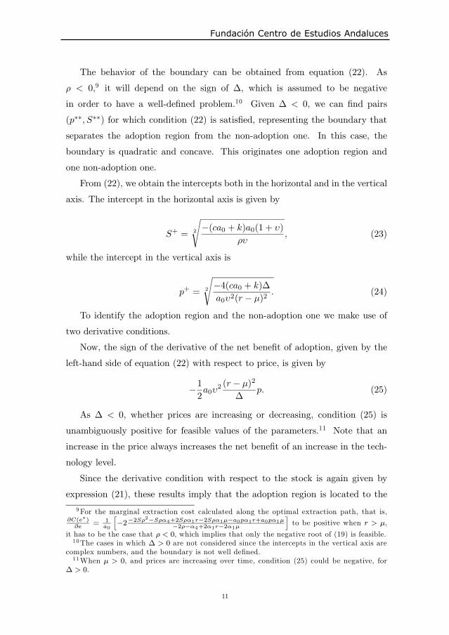
The behavior of the boundary can be obtained from equation (22). As

< 0,9 it will depend on the sign of , which is assumed to be negative

in order to have a well-defined problem.10

Given < 0, we can find pairs

(p , S ) for which condition (22) is satisfied, representing the boundary that

separates the adoption region from the non-adoption one. In this case, the

boundary is quadratic and concave. This originates one adoption region and

one non-adoption one.

From (22), we obtain the intercepts both in the horizontal and in the vertical

axis. The intercept in the horizontal axis is given by

S+ = 2

s(ca0 + k)a0(1 + )

, (23)

while the intercept in the vertical axis is

p+ = 2

s4(ca0 + k)

a02(r µ)2

. (24)

To identify the adoption region and the non-adoption one we make use of

two derivative conditions.

Now, the sign of the derivative of the net benefit of adoption, given by the

left-hand side of equation (22) with respect to price, is given by

1

2a0

2(r µ)2

p. (25)

As < 0, whether prices are increasing or decreasing, condition (25) is

unambiguously positive for feasible values of the parameters.11

Note that an

increase in the price always increases the net benefit of an increase in the tech-

nology level.

Since the derivative condition with respect to the stock is again given by

expression (21), these results imply that the adoption region is located to the

9For the marginal extraction cost calculated along the optimal extraction path, that is,

C(e )e

=1a0

h2

2S 2S 4+2S 1r 2S 1µ a0p 1r+a0p 1µ

2 4+2 1r 2 1µ

ito be positive when r > µ,

it has to be the case that < 0, which implies that only the negative root of (19) is feasible.10The cases in which > 0 are not considered since the intercepts in the vertical axis are

complex numbers, and the boundary is not well defined.11When µ > 0, and prices are increasing over time, condition (25) could be negative, for

> 0.


12

SS+

Adoption

region

No Adoption

region

p+

SS+

Adoption

region

No Adoption

region

p+

Figure 2: Adoption and Non-adoption Regions r > µ

right of the boundary and the non-adoption one to the left. Therefore, prices

are crucial to whether the firm chooses to adopt or not, as illustrated in Figure

2. As before, the larger the stock remaining at t = , the larger the net benefit

from adoption. Moreover, the higher the price at t = , the larger the benefit

from adoption.

For a given r, the impact of a change in µ on both the slope of the boundary

and the intercept p+depends on the sign of

µ. If

µ< 0, the higher the

price drift the steeper the boundary, implying that prices are less relevant for

the adoption choice decision. In the limit case, we are back in the case r = µ.

Therefore, the non-adoption region shrinks as µ decreases.12

Moreover, the

boundary is di erent between firms, depending upon the quality level operated

by each firm at t = . In particular, p+is lower and S

+is higher for larger

a0.13

By inspection of Fig. 2, we can observe that the adoption decision depends

on the exact location of the initial price and stock. It also depends on the price

12 Ifµ> 0, the result is ambiguous.

13 Ifµ< 0, the stock level is less relevant for the adoption decision at t = the lower is µ

and the higher is a0.

E2004/16

13

drift µ relative to the discount rate r, given the value of all the other parameters.

Therefore, we conclude that:

(a) when S > S+, the firm will decide to adopt, independently of prices;

(b) when S < S+, the decision to adopt depends on the price, namely, when

prices are high enough at t = , the firm will decide to adopt, while when prices

are low enough, the firm will decide not to adopt.

In this problem, as adoption reduces marginal extraction costs, and the even-

tual adoption at t = is unanticipated by the firm, the major force influencing

adoption behavior is the possibility of taking advantage of lower costs. There-

fore, the benefits from adoption increase with the resource stock remaining at

t = . In fact, for firms with more depleted stock levels, the technological op-

portunities can only be applied to a smaller amount of the stock, reducing net

benefits from adoption. As it is clear from the previous analysis, in order to be

optimal for a firm with a low stock level to choose adoption, prices have to be

high enough.

These results suggest that not only firms with depleted stocks will adopt.

Instead, we have shown that firms with large stocks are more likely to adopt,

independently of the price level, while firms with small stocks may choose not

to adopt if prices are low enough at t = .

3.1.2 Case 2: cost depends on the upgrading rate

In order to better understand the role played by prices and stock levels in the

adoption decision, the relationship between the intensity of the technological

upgrading, that is, the level of the upgrading rate, , and those variables is

examined. To this end, we consider a second case in which adoption costs depend

on the level of the upgrading rate, (c + k), rather than on the technology level

a0 (Case 1), besides the fixed cost, k, as before.

When r = µ, the condition for the firm to decide whether to adopt at t =

is given by

a0(1 + )S2

c k = 0. (26)

The optimal level of the upgrading rate, , is obtained by maximizing the

left-hand side of (26) with respect to , that is, by maximizing the net benefits


14

from adoption,

= S 2

rca0

1,

as strict concavity is guaranteed. The two derivative conditions with respect

to the stock and prices, respectively, that were derived for Case 1 still apply,

except that now the upgrading rate is evaluated at . SinceS= 2

qca0

is

always positive, firms with larger stocks at t = will optimally choose a larger

upgrading rate.

When r > µ, the condition for the firm to choose adoption is given by

a02(r µ)2

4p2

a0(1 + )S2

c k = 0. (27)

As before, the optimal level of the upgrading rate is obtained by maxi-

mizing the left-hand side of (27) with respect to .

By totally di erentiating the first-order conditions with respect to and

evaluating them at , and using the Implicit Function Theorem, we obtain

d

dS=

2

a0(1+ )2S

a0(r µ)2

2p2 +

a0(1+ )3S2

(28)

d

dp=

a0 (r µ)2

p

a0(r µ)2

2p2 +

a0(1+ )3S2. (29)

The second-order condition for a maximum requires that the denominator in

both (28) and (29) is negative, reflecting the fact that the marginal benefit of

the intensity of adoption decreases with the level of the upgrading rate. Hence,

the intensity of adoption increases with the level of the resource stock, as well

as with prices at t = .

3.2 Volatile prices

The results presented in this subsection are for the case of constant marginal

costs of adoption (Case 1). When facing volatile prices, the firm’s problem is

given by (1), and satisfies the following partial di erential equation:

rV =a0(p VS)

2

2 1

S 3(p VS)

2 1

[a0(p VS) S 3]2

4 1a0

2

a0S2(30)

S 3a0(p VS) S2 2

3

2 1a0+ µpVp +

1

2Vpp

2

pp2,

E2004/16

15

after substituting the optimal extraction for an interior solution.

We use the indeterminate coe cients method to obtain expressions for the

coe cients of the value function, in terms of the coe cients of the cost function,

as before. The solution is given by:

V (p, S; a0) =1

4a0

(r µ)2

+ 2p2 +

a0S2 +

2 + 3

2 2r 1 + 3 + 2µ 1

Sp (31)

where

= + 2( r + 2µ + 1r2

r 3 2 1rµ+ µ 3 + 1µ+ 2) =(32)

= + 2. (33)

Also, and are as before.

Again, it is useful to look separately at r = µ, and r > µ. Despite the fact

that prices are volatile, the uncertainty surrounding prices does not influence the

results for r = µ, as the term that incorporates the price volatility is eliminated.

It is as if the problem is deterministic when the firm chooses to optimally adopt

at t = . Therefore, for r = µ the solution is similar to the corresponding

deterministic one. Thus, in this section, we focus on r > µ.

The condition for the firm to decide about adoption at t = is now given

by

a02(r µ)2

4( + 2 )p2

a0(1 + )S2

ca0 k = 0, (34)

which depends both on the level of the stock, S, and prices, p. Thus, a rela-

tionship between S and p is derived, representing the boundary that separates

the adoption region from the non-adoption one.

The intercept in the horizontal axis is the same as in the deterministic case,

given by (24),while the intercept in the vertical axis is now given by

p+ = 2

s4(ca0 + k)( + 2 )

a02(r µ)2

. (35)

As < 0, the slope of the boundary separating the adoption region from

the non-adoption one depends on the sign of ( + 2 ), which is assumed to

be negative in order to have a well-defined problem. Given ( + 2 ) < 0, we

can find pairs (p , S ) for which condition (34) is satisfied, representing the


16

boundary that separates the adoption region from the non-adoption one. As

before, it is decreasing at a decreasing rate and it behaves similarly with respect

to the technology level a with which the firm operates.

To determine the location of the adoption and the nonadoption region, we

di erentiate the left-hand side of (34) with respect to both the stock and prices.

While the derivative condition for the stock is still given by equation (21), the

other for the resource price changes, and it is given by

1

2a0

2(r µ)2

+ 2p. (36)

By inspection, in the presence of price volatility, it is clear that S+does

not change. In contrast, p+(35) changes its position depending on the sign of

2 . As µ < 0 implies that 2 > 0, then p+decreases with

2. Consequently,

the rotation of the boundary implies that the adoption region is enlarged, while

the non-adoption one shrinks, reinforcing the e ect of decreasing prices relative

to the corresponding deterministic case. If µ > 0 and 2 > 0, the same

result occurs. However, as µ r, 2 < 0, and the price intercept increases,

determining an enlargement of the non-adoption region and a reduction of the

adoption one. Therefore, the e ect of increasing prices is reinforced relative to

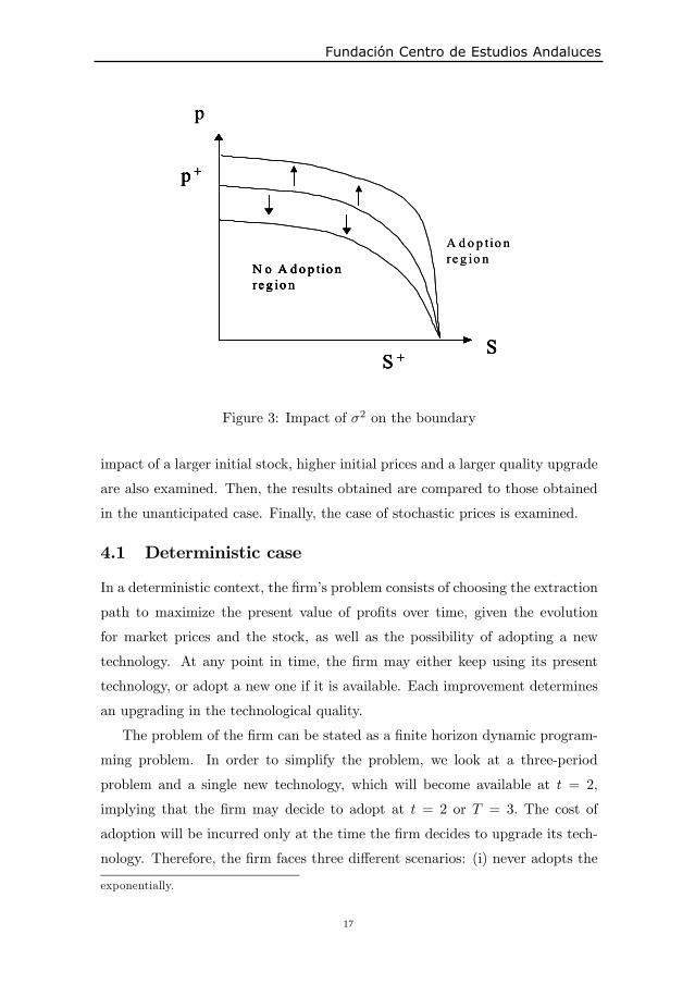
the corresponding deterministic case. Figure 3 illustrates these results both for

2 > 0 (boundary moving up) and 2 < 0 (boundary moving down).

4 Anticipated technological improvement

In contrast to previous sections, a general model of a competitive nonrenewable

resource extracting firm is used to analyze optimal extraction behavior and opti-

mal technology adoption of an incremental type, assuming that the availability

of a new technology is anticipated by the firm at the time the firm initiates

the extraction program, both in a deterministic and a stochastic context. The

solution to this problem is illustrated by solving numerically a dynamic pro-

gramming problem for a time horizon of three periods, as it is not possible to

solve analytically the adoption problem of the firm when it has simultaneously

to decide at each time period how much to extract of the resource stock.14The

14We only use one technological improvement for simplicity. If at each time period a new

technology became available, the number of alternative adoption sequences would increase

E2004/16

17

SS +

N o A d o p tio n

re g io n

p +

SS +

A d o p tio n

re g io nN o A d o p tio n

re g io n

p +

p

SS +

N o A d o p tio n

re g io n

p +

SS +

A d o p tio n

re g io nN o A d o p tio n

re g io n

p +

p

Figure 3: Impact of2on the boundary

impact of a larger initial stock, higher initial prices and a larger quality upgrade

are also examined. Then, the results obtained are compared to those obtained

in the unanticipated case. Finally, the case of stochastic prices is examined.

4.1 Deterministic case

In a deterministic context, the firm’s problem consists of choosing the extraction

path to maximize the present value of profits over time, given the evolution

for market prices and the stock, as well as the possibility of adopting a new

technology. At any point in time, the firm may either keep using its present

technology, or adopt a new one if it is available. Each improvement determines

an upgrading in the technological quality.

The problem of the firm can be stated as a finite horizon dynamic program-

ming problem. In order to simplify the problem, we look at a three-period

problem and a single new technology, which will become available at t = 2,

implying that the firm may decide to adopt at t = 2 or T = 3. The cost of

adoption will be incurred only at the time the firm decides to upgrade its tech-

nology. Therefore, the firm faces three di erent scenarios: (i) never adopts the

exponentially.


18

new technology, (ii) adopts at t = 2, implying that it will keep it at T = 3,

and, finally (iii) waits and only adopts at T = 3. The profits associated with

each scenario can be calculated, and the scenario with highest profit will be the

optimal choice.

In recursive form, the problem for a time horizon of T = 3 periods can be

stated as follows. In all cases, the stock St represents the stock that remains at

the beginning of period t. Since the resource is exhausted at the final period,

the stock at the beginning of the final period is equal to the amount extracted

in that period, and it will be obtained residually. Also, hereafter, NA stands

for no adoption, and A for adoption, where the upgrade in technology is given

by

a0 = (1 + v)a.

For scenario (i), in which the firm never adopts, the problem consists of

choosing the extraction path that maximizes present value of profits given that:

• t = T = 3 :

V3(S3, p3; NA) =Maxe3

{ (S3, p3; a)}

• t = 2 :

V2(S2, p2, NA;NA) =Maxe2

{ (S2, p2; a) + V3(·)}

s.t S3 = S2 e2

p3 = (1 + µ)p2

• t = 1 :

V1(S1, p1, NA;NA,NA) =Maxe1

{ (S1, p1; a) + V2(·)}

s.t S2 = S1 e1

p2 = (1 + µ)p1

where the initial stock, S1, and prices, p1, are given.

A similar problem can be stated for scenario (ii), where the firm decides to

adopt at t = 2, switching technology from a to a0 at that moment and incurring

in an adoption cost of ca+k, as well as for scenario (iii), where the firm decides

to adopt only at T = 3 (see Appendix B). The optimal solution is given by the

scenario for which V1(.) is highest, given the initial conditions on prices and the

stock. Thus, once V1(.) is chosen the optimal pattern of adoption is identified.

E2004/16

19

4.1.1 Numerical example

The numerical example is solved by applying the procedure described for a

three-period horizon, T = 3, and is based on a quadratic cost function as be-

fore. Moreover, the conditions of the problem are such that the transversality

conditions for the stock are satisfied when the resource is exhausted at the final

period.15

The chosen parameters for the cost function are 1 = 4, 2 = 0.1, and

4 = 1.25. As can be easily checked, for these values of the parameters the

cost function is strictly convex. Moreover, we assume that the discount rate

is 5%, r = 0.05, and the drift term on prices is 2%, µ = 0.02. Also, in the

benchmark case, S(1) = 150, p(1) = 33.641, c = 5, k = 10, and a = 10.

Assuming = 0.09, the upgraded technology quality level is a0 = 10.9 (see

Appendix D, Table 1A).

For the values of the parameters in the benchmark case, the problem of the

firm was solved separately for each scenario. The optimal solution corresponds

to the scenario that maximizes the value of the firm at t = 1, which in this

case is scenario (ii), implying that the firm decides to adopt at t = 2. As

expected, when the firm anticipates the possibility of adopting in the future, it

will act strategically by saving resource to the future. Thus, the lowest amount

extracted at the initial period is obtained in the optimal scenario. If the firm

did not anticipate the chance of adopting in the future, it would choose to

extract in the initial period the amount obtained in scenario (i), as the solution

of scenario (i) in the first period corresponds to the solution for a firm that does

not anticipate the event of any technology adoption. Consequently, it is higher

than in the optimal scenario. (see Appendix D, Table 1B).

The results in the benchmark problem were compared to those obtained in

di erent cases: a larger upgrading rate ( = 0.3) (see Appendix D, Table 5),

higher initial prices (p(1) = 43.523) (see Appendix D, Table 4), and, finally, a

change in the stock endowment (a lower and a larger initial stock; see Appendix

D, Tables 2 and 3). With a higher initial price and a larger upgrading rate,

the optimal scenario is the same as before. As expected, a larger upgrading

15The marginal user cost is positive for all periods, see Appendix C.


20

rate reinforces the importance of technology upgrades on extraction. Thus, the

largest decrease in extraction in the initial period occurs in the optimal scenario,

and the highest increase in extraction in the final period in scenario (iii). With

higher initial prices or a more highly valued resource, the amounts extracted

are always larger in the initial period and lower in the final period than in the

benchmark case. Therefore, the e ect of higher prices on extraction in the initial

period reduces the impact of innovation, reducing the incentive to save to the

future. Also, the benefits from adoption increase. Comparing now the results

obtained when the initial stock changes, we observe that when the resource

stock increases to S(1) = 165, the optimal scenario is the same, and benefits

from adoption increase. In contrast, when the stock is reduced to S(1) = 65,

the optimal scenario changes, as the firm’s optimal decision is to never adopt.

However, for S(1) = 65, the firm will adopt if prices are high enough, as we

show in the next subsection. These results are in line with those previously

obtained, according to which (i) larger stocks and higher prices make adoption

more profitable for the firm, (ii) large stocks lead to adoption independently of

prices, and (iii) low stocks with high enough prices may induce adoption.

4.2 Stochastic case

In this subsection, we assume that there is uncertainty about the evolution of

the price of the resource. That is, either prices increase at a rate 0 < µ < r

with probability q, or do not change (µ = 0) with probability (1 q). Moreover,

the technological improvement becomes available at the initial period, implying

that the firm may either decide to adopt immediately or to postpone adoption.16

Therefore, the problem can be stated as follows:

For scenario (i), in which the firm never adopts, we have for T = 3 :

• t = T = 3 :

V3(S3, p3; NA) =Maxe3

{ (S3, p3; a)}

16 Since there are only three periods, and the decision on extraction in the last period

is residual, in order to capture the eventual decision to delay adoption, the technological

improvement has to become available already in the initial period, rather than only on the

second one, as in the deterministic case.

E2004/16

21

or,

V3(S3, p03; NA) =Max

e3

{ (S3, p03; a)}

• t = 2 : 17

V2(S2, p2, q,NA;NA) =Maxe2

{ (S2, p2; a) + V3(S3, p3;NA)} (37)

or,

V2(S2, p02, q,NA;NA) =Max

e2

{ (S2, p02; a) + V3(S3, p

03;NA)} (38)

• t = 1 :

The problem in this period must be solved considering the uncertainty in

future prices. Therefore, we have

V1(S1, p1, q) = Maxe2

{ (S1, p1; a) +

+ [qV2(S2, p02;NA,NA) + (1 q)V2(S2, p2;NA,NA)]}

subject to the stock transition, where p03= (1 + µ)p0

2, p

02= (1 + µ)p1 for

µ > 0, and p3 = p2 = p1.

Analogous recursive problems can be written for scenarios (ii) and (iii). In

the case of scenario (ii), the problem is similar to the deterministic one, except

that the firm adopts in the first period. Thus, for

• t = 1 :

V1(S1, p1, q) = Maxe2

{ (S1, p1; a0) ca k +

+ [qV2(S2, p02;A,A) + (1 q)V2(S2, p2;A,A)]}

subject to the stock transition, where p03= (1 + µ)p0

2, p

02= (1 + µ)p1 for

µ > 0, and p3 = p2 = p1, as before (see Appendix B).

In the case of scenario (iii), there are di erent alternatives to be considered

(see Appendix B), as the decision to adopt may depend upon the realization of

uncertainty. The alternative presented below, labeled V5

1(S1, p1, q), is the one

that maximizes the initial value when solving for the example. Thus,

17We are assuming, for simplicity, that all the uncertainty is solved at t = 2.


22

• t = 1 :

V5

1(S1, p1, q) = Max

e2

{ (S1, p1; a) +

+ [qV2(S2, p02;A,A) + (1 q)V2(S2, p2;NA,NA)]}

Solving this problem for S(1) = 65, p1 = p2 = p3 = 75, p03= 99.188,

p02= 86.25, p1 = 75, for µ = 0.15 and r = 0.2, we obtain that the optimal

solution is scenario (ii), or to adopt at t = 1 if q > 0.05, but it is scenario (iii)

if q = 0.03. That is, with uncertain benefits from adoption the firm prefers to

wait and adopt later rather than adopt immediately. The corresponding optimal

values for the initial period are: V1= 4066.4 in scenario (i), V

1= 4057.7 in

scenario (ii), and V1= 4072 in scenario (iii) in the case described. For q = 0

the firm decides not to adopt (scenario (i)), while for q = 1 decides to adopt at

t = 1 (scenario (ii)).

5 Conclusions

Empirical research shows that the role played by technology adoption in the

natural resource industry is considered to be the determinant factor in extrac-

tion cost decrease, responding to the continuing search for lower costs in a

competitive market.

In this paper, the optimal extraction and technology adoption decisions are

modeled for a competitive nonrenewable resource extracting firm, both in a

deterministic and in a stochastic environment, when the firm either anticipates

adoption or not. It is assumed that better technology reduces the marginal

cost of production but has a known adoption cost. Thus, at the time the new

technology is available, adoption will only occur if net benefits are positive.

In the unanticipated case a boundary separating the adoption region from the

non-adoption one is defined.

In the presence of a resource stock, with a quadratic cost function, we show

that the main driving force of adoption is the possibility of taking advantage of

lower costs. In fact, for firms with more depleted stock levels, the technological

opportunities can only be applied to a smaller amount of the stock, reducing

E2004/16

23

net benefits from adoption. In order for a firm with a low stock level to choose

to adopt, prices have to be high enough. Therefore, the price level is also crucial

to the adoption/non-adoption decision.

If adoption costs depend on the level of the upgrading rate and the firm

does not anticipate the technological improvement, as the marginal benefit of

the upgrading rate is positive with respect to both the stock level and prices,

firms choosing lower intensity levels are those with more depleted stocks and

facing lower prices. Therefore, the level of prices turns out to be crucial not

only to the adoption decision, but also to the optimal choice of the intensity

of adoption in the presence of a nonrenewable resource. In this context, we

may reinterpret some of the results in Pindyck [12] on exploratory e ort. When

reserves are large and prices are steadily increasing, as the exploratory e ort

is never enough to compensate for extraction, reserves will be decreasing over

time, as in our case. The path for the exploratory e ort, increasing first and

then decreasing, can be interpreted in terms of our results as the firm choosing

higher intensity of adoption when reserves are large, suggesting that benefits

from adoption are larger for large stocks, as exploratory e ort is more intense

when reserves are large.

With price volatility, the adoption decision is also a ected by the variance

of price. With increasing prices, volatility tends to make adoption less likely,

while for decreasing prices the opposite occurs.

Finally, for the case of anticipated technological improvements, the extrac-

tion decision of the firm changes for the entire planning horizon, as adoption

decisions are incorporated from the start. The problem is solved numerically

for a three-period dynamic programming problem, in order to solve simultane-

ously for the optimal extraction and optimal timing of adoption. As expected,

the firm acts strategically, reducing extraction in the initial period, in order to

save resource for the future when the possibility of adoption is presented. As in

the unanticipated case, the benefits for the firm increase with the stock as well

as with prices. Moreover, with su ciently large stocks the adoption decision

does not depend on prices. In contrast, for low stocks, the firm may decide to

adopt only when prices are high enough. When benefits from adoption are un-


24

certain, namely by assuming that the evolution of resource prices is uncertain,

the firm may decide to wait and adopt only if prices increase rather than adopt

immediately.

E2004/16

25

A Characterization of optimal paths

A.1 For the case r = µ

In this case, V (.) is given by

V (p, S; a) =a0S2 + Sp.

When S = 0, the transversality condition holds

V (p, 0; a0) = 0.

Moreover, along the optimal path for extraction, that is, for

e =2 + 4

2 1

S,

we can show that the marginal extraction cost is driven to zero when S = 0.

For S > 0, the marginal extraction cost is always positive.

As expected, the marginal opportunity cost of the resource is always positive,

for p > 0, when S = 0, as VS = p. For any S > 0, the opportunity cost is positive

as long as p >2

a0S; in particular, for the initial stock p0 >

2

a0S0.

Therefore, the transversality condition for the stock holds as limt

VSt exp( rt) =

p0 > 0, since r = µ, implying that limt

VSt exp( rt)St = 0 as limt

St 0.

A.2 For the case r > µ

Now the optimal extraction policy for an interior solution is given by

e =2 + 4

2 1

Sa0(r µ)

2 + 4 2 1(r µ)p

As expected, the opportunity cost of the resource is always positive, for

p > 0, when S = 0, as follows:

VS =2 + 4

2 2r 1 + 4 + 2µ 1

p

for values of the parameters that satisfy all the relevant conditions.

For any S > 0, the opportunity cost is positive as long as


26

p >

2

a0

2 + 4

2 2r 1+ 4+2µ 1

S

and, in particular, for S0,

p0 >

2

a0

2 + 4

2 2r 1+ 4+2µ 1

S0,

which is always satisfied for values of the parameters that verify all the relevant

conditions.

Therefore, the transversality condition for the stock is limt

VSt exp( rt)St =

0. As VSt exp( rt) approaches zero at a rate r µ, if the stock approaches zero

at least at the same rate the transversality condition is satisfied.

A.3 Volatile prices: case r > µ

The optimal extraction policy for an interior solution is given by

e =2 + 4

2 1

Sa0(r µ)

2 + 4 2 1(r µ)p

As expected, the opportunity cost of the resource is always positive, for

p > 0, when S = 0, as follows

VS =2 + 4

2 2r 1 + 4 + 2µ 1

p

for values of the parameters that satisfy all the relevant conditions.

For any S > 0, the opportunity cost is positive as long as

p >

2

a0

2 + 4

2 2r 1+ 4+2µ 1

S

and, in particular, for S0,

p0 >

2

a0

2 + 4

2 2r 1+ 4+2µ 1

S0,

which is always satisfied for values of the parameters that verify all the relevant

conditions. As before, the transversality condition for the stock holds in the

above conditions.

E2004/16

27

B.1 Deterministic case

For scenario (ii), the firm adopts at t = 2 so we have:

• t = T = 3 : V3(S3, p3; A) =Maxe3

{ (S3, p3; a0)}

where a0 = a(1 + ).

• t = 2 : V2(S2, p2, A;A) =Maxe2

{ (S2, p2; a0) ca k + V3(·)}

subject to the transitions for the stock and prices, as before.

• t = 1 : V1(S1, p1, NA;A,A) =Maxe1

{ (S1, p1; a) + V2(·)}

where the initial stock, S1, and prices, p1, are given, and the transition

equations are taken into account.

Finally, for scenario (iii), where the firm decides to adopt only at T = 3, the

problem consists of:

• t = T = 3 : V3(S3, p3; A) =Maxe3

{ (S3, p3; a0) ca k}

• t = 2 : V2(S2, p2, NA;A) =Maxe2

{ (S2, p2; a) + V3(·)}

subject to the transitions for stock and prices.

• t = 1 : V1(S1, p1, NA;NA,A) =Maxe1

{ (S1, p1; a) + V2(·)}

again subject to the transitions for stock and prices, given S1 and p1.

B.2 Stochastic case

For scenario (ii), where the firm decides to adopt at t = 1:

• t = T = 3 : V3(S3, p3; A) = Maxe3

{ (S3, p3; a0)} or V3(S3, p

03; A) =

Maxe3

{ (S3, p03; a0)}.

• t = 2 : V2(S2, p2, A;A) =Maxe2

{ (S2, p2; a0)+ V3(S3, p3;A)} or V2(S2, p

02, A;A) =

Maxe2

{ (S2, p02; a0) + V3(S3, p

03;A)}.


28

• t = 1 :

V1(S1, p1; q) =Maxe1

{ (S1, p1; a0) ca k+

+ [qV2(S2, p02;A,A) + (1 q)V2(S2, p2;A,A)]}

where the initial stock, S1, and prices, p1, are given, satisfying the two

transitions, respectively.

Finally, for scenario (iii), where the firm decides to adopt at t = 2 or T = 3,

the problem consists of:

• t = T = 3 : V3(S3, p3; A) =Maxe3

{ (S3, p3; a0) ca k} or

V3(S3, p03; A) =Max

e3

{ (S3, p03; a0) ca k} or

V3(S3, p3; A) =Maxe3

{ (S3, p3; a0)} or

V3(S3, p03; A) =Max

e3

{ (S3, p03; a0)}.

• t = 2 :

V2(S2, p02, A;A) =Max

e2

{ (S2, p02; a0) ca k + V3(S3, p

03;A),

or

V2(S2, p2, A;A) =Maxe2

{ (S2, p2; a0) ca k + V3(S3, p3; A)}

or

V2(S2, p02, NA;A) =Max

e2

{ (S2, p02; a) + V3(S3, p

03;A),

and

V2(S2, p2, NA;A) =Maxe2

{ (S2, p2; a) + V3(S3, p3;A),

subject to the transitions for the stock and prices. The alternative of not

adopting both in t = 2 and T = 3 was already derived in scenario (i).

• t = 1 :

V1

1(S1, p1; q) = Max

e1

{ (S1, p1; a) +

+ [qV2(S2, p02, q;A,A) + (1 p)V2(S2, p2, q;A,A)]}

E2004/16

29

or

V2

1(S1, p1; q) = Max

e1

{ (S1, p1; a) +

+ [qV2(S2, p02, q;NA,A) + (1 p)V2(S2, p2, q;A,A)]}

or

V3

1(S1, p1; q) = Max

e1

{ (S1, p1; a) +

+ [qV2(S2, p02, q;NA,NA) + (1 p)V2(S2, p2, q;A,A)]}

or

V4

1(S1, p1; q) = Max

e1

{ (S1, p1; a) +

+ [qV2(S2, p02, q;A,A) + (1 p)V2(S2, p2, q;NA,A)]}

or

V5

1(S1, p1; q) = Max

e1

{ (S1, p1; a) +

+ [qV2(S2, p02, q;A,A) + (1 p)V2(S2, p2, q;NA,NA)]}

subject to the transitions for the stock and prices, given S1 and p1. The

other alternative of never adopting was already obtained in scenario (i).

C Marginal user cost of the resource in the an-

ticipated problem

The marginal user cost at each time period can be derived by using the Envelope

Theorem at each time period. Thus, at T = 3, we obtain:

V3

S3=

1

a(2 2S3 + 4e3)

or,

V3

S3=

1

ae3(2 2 + 4).

since is evaluated at the optimum. Therefore, the marginal user costV3

S3> 0

as long as 4

2 2

> 1, which is satisfied for the values of the parameters of the

cost function.


30

At t = 2, the marginal user cost is given by

V2

S2=

1

a(2 2S2 + 4e2) +

V3

S3.

Given thatV3

S3> 0, then a su cient condition for

V2

S2> 0 is that 4

2 2

>S2

e2,

which always hold as well.

Finally, by following a similar procedure, a su cient condition for the marginal

user cost in period t = 1, V1

S1, to be positive is that 4

2 2

>S1

e1, which also holds.

In summary, the su cient conditions for exhaustion in the above problem

are that 4

2 2

>St

et, for t = 1, 2, 3.

Based on a similar argument, one can show that the same holds in the

stochastic case.

D Tables for the numerical example

Table 1A

Benchmark Case

S(1) 150p1 33. 641µ 0.02r 0.05a 10

0.09a0 10.9c 5k 10

Table 1B

Solution (Benchmark Case) scenario (i) scenario (ii) scenario (iii)

e1

52.38 50.338 51.22

e2

49.28 50.362 48.168

e3

48.34 49.3 50.612

V1

3519.64 3551.04 3517.62

V2

2202. 6 2259. 9 2214.0V3

1025.9 1090 1041.7

E2004/16

31

Table 2

Solution S(1) = 65 scenario (i) scenario (ii) scenario (iii)

e1

23.046 22.262 23.109

e2

21.596 21.872 20.862

e3

20.358 20.506 21.029

V1

1866.2 1825.1 1820.9

Table 3

Solution S(1) = 165 scenario (i) scenario (ii) scenario (iii)

e1

57.557 55.228 56.181

e2

54.166 55.39 52.987

e3

53.277 54.382 55.832

V1

2117.64 3769.29 3728.35

Table 4

Solution p1 = 43.253 scenario (i) scenario (ii) scenario (iii)

e1

52.555 50.746 51.682

e2

49.402 50.386 48.162

e3

48.043 48.868 50.156

V1

4921. 7 4952.4 4918. 8

Table 5

Solution a0 = 13 scenario (i) scenario (ii) scenario (iii)

e1

52.38 46.988 49.055

e2

49.28 52.181 45.789

e3

48.34 50.831 55.156

V1

3519.64 3718.3 3625.0


32

References

[1] Y. Balcer and S. A. Lippman, Technological Expectations and Adoption of

Improved Technology, Journal of Economic Theory 34, 292-318 (1984).

[2] D. Bertsekas, Dynamic Programming, Deterministic and Stochastic Mod-

els, Prentice-Hall, 1987.

[3] P. Dasgupta, Natural Resources in an Age of Substitutability, in “Hand-

book of Natural Resource and Energy Economics” (A. V. Kneese and J. L.

Sweeney, Eds.), Vol. III, Elsevier Science Publishers B.V. (1993).

[4] A. Dixit and R. Pindyck, Investment under Uncertainty, Princeton Univer-

sity Press, Princeton, NJ, 1994.

[5] U. Doraszelski, Innovations, Improvements, and the Optimal Adoption of

New Technologies, Journal of Economic Dynamics and Control, forthcom-

ing.

[6] Y. H. Farzin, Technological Change and the Dynamics of Resource Scarcity

Measures, Journal of Environmental Economics and Management 29, 105-

120 (1995).

[7] Y. Farzin, K. Huisman, and P. Kort, Optimal Timing of Technology Adop-

tion, Journal of Economic Dynamics and Control 22:779-799, 1998.

[8] B. Hall and B. Khan, Adoption of New Technology , Working-Paper #9730,

NBER, May 2003.

[9] J. Krautkraemer, Nonrenewable Resource Scarcity, Journal of Economic

Literature, Vol. XXXVI, 2065-2107 (1998).

[10] S. Lundstrom, Cycles of Technology, Natural Resources and Economic

Growth, mimeo, Department of Economics, Goteborg University, June

2002.

[11] S. Managi, James J. Opaluch, Di Jin and T. A. Grigalunas, Journal of

Environmental Economics and Management, forthcoming.

E2004/16

33

[12] Robert S. Pindyck, The Optimal Exploration and Production of Nonre-

newable Resources, Journal of Political Economy, Vol. 86, # 5 (1978).

[13] Robert S. Pindyck, Optimal Timing Problems In Environmental Eco-

nomics, Journal of Economics, Dynamics & Control 26, 1677-1697 (2002).

[14] R. D. Simpson, Technological Innovation in Natural Resource Industries,

in “Productivity in Natural Resource Industries” (R. D. Simpson, Ed. ),

Resources for the Future (1999).

[15] J. Tilton and H. Landsberg, Innovation, Productivity Growth, and the Sur-

vival of the U.S. Copper Industry, Discussion Paper 97-41, RFF, September

1997.



Documentos de Trabajo

Serie Economía

E2001/01 “The nineties in Spain: so much flexibility in the labor market?’’,J. Ignacio García Pérez y Fernando Muñoz Bullón.

E2001/02 “A Log-linear Homotopy Approach to Initialize the ParameterizedExpectations Algorithm’’, Javier J. Pérez.

E2001/03 “Computing Robust Stylized Facts on Comovement’’, Francisco J.André, Javier J. Pérez, y Ricardo Martín.

E2001/04 “Linking public investment to private investment. The case of theSpanish regions”, Diego Martínez López.

E2001/05 “Price Wars and Collusion in the Spanish Electricity Market”, JuanToro y Natalia Fabra.

E2001/06 “Expedient and Monotone Learning Rules”, Tilman Börgers,Antonio J. Morales y Rajiv Sarin.

E2001/07 “A Generalized Production Set. The Production and RecyclingFunction”, Francisco J. André y Emilio Cerdá.

E2002/01 “Flujos Migratorios entre provincias andaluzas y entre éstas y elresto de España’’, J. Ignacio García Pérez y Consuelo GámezAmián.

E2002/02 “Flujos de trabajadores en el mercado de trabajo andaluz’’, J.Ignacio García Pérez y Consuelo Gámez Amián.

E2002/03 “Absolute Expediency and Imitative Behaviour”, Antonio J.Morales Siles.

E2002/04 “Implementing the 35 Hour Workweek by means of OvertimeTaxation”, Victoria Osuna Padilla y José-Víctor Ríos-Rull.

E2002/05 “Landfilling, Set-Up costs and Optimal Capacity”, Francisco J.André y Emilio Cerdá.

E2002/06 “Identifying endogenous fiscal policy rules for macroeconomicmodels”, Javier J. Pérez y Paul Hiebert.

E2002/07 “Análisis dinámico de la relación entre ciclo económico y ciclo deldesempleo en Andalucía en comparación con el resto de España”,Javier J. Pérez, Jesús Rodríguez López y Carlos Usabiaga.

E2002/08 “Provisión eficiente de inversión pública financiada conimpuestos distorsionantes”, José Manuel González-Páramo yDiego Martínez López.

E2002/09 “Complete or Partial Inflation convergence in the EU?”, ConsueloGámez y Amalia Morales-Zumaquero.

E2002/10 “On the Choice of an Exchange Regime: Target Zones Revisited”,Jesús Rodríguez López y Hugo Rodríguez Mendizábal.

E2002/11 “Should Fiscal Policy Be Different in a Non-CompetitiveFramework?”, Arantza Gorostiaga.

E2002/12 “Debt Reduction and Automatic Stabilisation”, Paul Hiebert,Javier J. Pérez y Massimo Rostagno.

E2002/13 “An Applied General Equilibrium Model to Assess the Impact ofNational Tax Changes on a Regional Economy”, M. AlejandroCardenete y Ferran Sancho.

E2002/14 “Optimal Endowments of Public Investment: An EmpiricalAnalysis for the Spanish Regions”, Óscar Bajo Rubio, CarmenDíaz Roldán y M. Dolores Montávez Garcés.

E2002/15 “Is it Worth Refining Linear Approximations to Non-LinearRational Expectations Models?” , Alfonso Novales y Javier J.Pérez.

E2002/16 “Factors affecting quits and layoffs in Spain”, Antonio CaparrósRuiz y M.ª Lucía Navarro Gómez.

E2002/17 “El problema de desempleo en la economía andaluza (1990-2001): análisis de la transición desde la educación al mercadolaboral”, Emilio Congregado y J. Ignacio García Pérez.

E2002/18 “Pautas cíclicas de la economía andaluza en el período 1984-2001: un análisis comparado”, Teresa Leal, Javier J. Pérez yJesús Rodríguez.

E2002/19 “The European Business Cycle”, Mike Artis, Hans-Martin Krolzig yJuan Toro.

E2002/20 “Classical and Modern Business Cycle Measurement: TheEuropean Case”, Hans-Martin Krolzig y Juan Toro.

E2002/21 “On the Desirability of Supply-Side Intervention in a MonetaryUnion”, Mª Carmen Díaz Roldán.

E2003/01 “Modelo Input-Output de agua. Análisis de las relacionesintersectoriales de agua en Andalucía”, Esther Velázquez Alonso.

E2003/02 “Robust Stylized Facts on Comovement for the SpanishEconomy”, Francisco J. André y Javier Pérez.

E2003/03 “Income Distribution in a Regional Economy: A SAM Model”,Maria Llop y Antonio Manresa.

E2003/04 “Quantitative Restrictions on Clothing Imports: Impact andDeterminants of the Common Trade Policy Towards DevelopingCountries”, Juliette Milgram.

E2003/05 “Convergencia entre Andalucía y España: una aproximación a suscausas (1965-1995). ¿Afecta la inversión pública al crecimiento?”,Javier Rodero Cosano, Diego Martínez López y Rafaela PérezSánchez.

E2003/06 “Human Capital Externalities: A Sectoral-Regional Application forSpain”, Lorenzo Serrano.

E2003/07 “Dominant Strategies Implementation of the Critical PathAllocation in the Project Planning Problem”, Juan Perote Peña.

E2003/08 “The Impossibility of Strategy-Proof Clustering”, Javier PerotePeña y Juan Perote Peña.

E2003/09 “Plurality Rule Works in Three-Candidate Elections”, BernardoMoreno y M. Socorro Puy.

E2003/10 “A Social Choice Trade-off Between Alternative FairnessConcepts: Solidarity versus Flexibility”, Juan Perote Peña.

E2003/11 “Computational Errors in Guessing Games”, Pablo Brañas Garzay Antonio Morales.

E2003/12 “Dominant Strategies Implementation when Compensations areAllowed: a Characterization”, Juan Perote Peña.

E2003/13 “Filter-Design and Model-Based Analysis of Economic Cycles”,Diego J. Pedregal.

E2003/14 “Strategy-Proof Estimators for Simple Regression”, Javier PerotePeña y Juan Perote Peña.

E2003/15 “La Teoría de Grafos aplicada al estudio del consumo sectorial deagua en Andalucía", Esther Velázquez Alonso.

E2003/16 “Solidarity in Terms of Reciprocity", Juan Perote Peña.

E2003/17 “The Effects of Common Advice on One-shot Traveler’s DilemmaGames: Explaining Behavior through an Introspective Model withErrors", C. Monica Capra, Susana Cabrera y Rosario Gómez.

E2003/18 “Multi-Criteria Analysis of Factors Use Level: The Case of Waterfor Irrigation", José A. Gómez-Limón, Laura Riesgo y ManuelArriaza.

E2003/19 “Gender Differences in Prisoners’ Dilemma", Pablo Brañas-Garzay Antonio J. Morales-Siles.

E2003/20 “Un análisis estructural de la economía andaluza a través dematrices de contabilidad social: 1990-1999", M. Carmen Lima,M. Alejandro Cardenete y José Vallés.

E2003/21 “Análisis de multiplicadores lineales en una economía regionalabierta", Maria Llop y Antonio Manresa.

E2003/22 “Testing the Fisher Effect in the Presence of Structural Change:A Case Study of the UK", Óscar Bajo-Rubio, Carmen Díaz-Roldány Vicente Esteve.

E2003/23 "On Tests for Double Differencing: Some Extensions and the Roleof Initial Values", Paulo M. M. Rodrigues y A. M. Robert Taylor.

E2003/24 "How Tight Should Central Bank’s Hands be Tied? Credibility,Volatility and the Optimal Band Width of a Target Zone", JesúsRodríguez López y Hugo Rodríguez Mendizábal.

E2003/25 "Ethical implementation and the Creation of Moral Values", JuanPerote Peña.

E2003/26 "The Scoring Rules in an Endogenous Election", Bernardo Morenoy M. Socorro Puy.

E2003/27 "Nash Implementation and Uncertain Renegotiation", PabloAmorós.

E2003/28 "Does Familiar Environment Affect Individual Risk Attitudes?Olive-oil Producer vs. no-producer Households", FranciscaJiménez Jiménez.

E2003/29 "Searching for Threshold Effects in the Evolution of BudgetDeficits: An Application to the Spanish Case", Óscar Bajo-Rubio,Carmen Díaz-Roldán y Vicente Esteve.

E2003/30 "The Construction of input-output Coefficients Matrices in anAxiomatic Context: Some Further Considerations", Thijs ten Raay José Manuel Rueda Cantuche.

E2003/31 "Tax Reforms in an Endogenous Growth Model with Pollution",Esther Fernández, Rafaela Pérez y Jesús Ruiz.

E2003/32 "Is the Budget Deficit Sustainable when Fiscal Policy isnonlinear? The Case of Spain, 1961-2001", Óscar Bajo-Rubio,Carmen Díaz-Roldán y Vicente Esteve.

E2003/33 "On the Credibility of a Target Zone: Evidence from the EMS",Francisco Ledesma-Rodríguez, Manuel Navarro-Ibáñez, JorgePérez-Rodríguez y Simón Sosvilla-Rivero.

E2003/34 "Efectos a largo plazo sobre la economía andaluza de las ayudasprocedentes de los fondos estructurales: el Marco de ApoyoComunitario 1994-1999", Encarnación Murillo García y SimónSosvilla-Rivero.

E2003/35 “Researching with Whom? Stability and Manipulation”, JoséAlcalde y Pablo Revilla.

E2003/36 “Cómo deciden los matrimonios el número óptimo de hijos”,Francisca Jiménez Jiménez.

E2003/37 “Applications of Distributed Optimal Control in Economics.The Case of Forest Management”, Renan Goetz y AngelsXabadia.

E2003/38 “An Extra Time Duration Model with Application toUnemployment Duration under Benefits in Spain”, José MaríaArranz y Juan Muro Romero.

E2003/39 “Regulation and Evolution of Harvesting Rules and Compliance inCommon Pool Resources”, Anastasios Xepapadeas.

E2003/40 “On the Coincidence of the Feedback Nash and StackelbergEquilibria in Economic Applications of Differential Games”,Santiago J. Rubio.

E2003/41 “Collusion with Capacity Constraints over the Business Cycle”,Natalia Fabra.

E2003/42 “Profitable Unproductive Innovations”, María J. Álvarez-Peláez,Christian Groth.

E2003/43 “Sustainability and Substitution of Exhaustible NaturalResources. How Resource Prices Affect Long-Term R&D-Investments”, Lucas Bretschger, Sjak Smulders.

E2003/44 “Análisis de la estructura de la inflación de las regionesespañolas: La metodología de Ball y Mankiw”, María ÁngelesCaraballo, Carlos Usabiaga.

E2003/45 “An Empirical Analysis of the Demand for Physician ServicesAcross the European Union”, Sergi Jiménez-Martín, José M.Labeaga, Maite Martínez-Granado.

E2003/46 “An Exploration into the Effects of Fiscal Variables on RegionalGrowth”, Diego Martínez López.

E2003/47 “Teaching Nash Equilibrium and Strategy Dominance: AClassroom Experiment on the Beauty Contest”. Virtudes AlbaFernández, Francisca Jiménez Jiménez, Pablo Brañas Garza,Javier Rodero Cosano.

E2003/48 "Environmental Fiscal Policies Might be Ineffective to ControlPollution", Esther Fernández, Rafaela Pérez y Jesús Ruiz.

E2003/49 "Non-stationary Job Search When Jobs Do Not Last Forever: AStructural Estimation to Evaluate Alternative UnemploymentInsurance Systems", José Ignacio García Pérez.

E2003/50 “Poverty in Dictator Games: Awakening Solidarity”, PabloBrañas-Garza.

E2003/51 “Exchange Rate Regimes, Globalisation and the Cost of Capital inEmerging Markets” Antonio Díez de los Ríos.

E2003/52 “Opting-out of Public Education in Urban Economies”. FranciscoMartínez Mora.

E2004/01 “Partial Horizontal Inequity Orderings: A non-parametricApproach”, Juan Gabriel Rodríguez, Rafael Salas, IrenePerrote.

E2004/02 “El enfoque microeconómico en la estimación de la demanda detransporte de mercancías. Análisis desde una perspectivaregional”, Cristina Borra Marcos, Luis Palma Martos.

E2004/03 “El marco del SEC95 y las matrices de contabilidad social:España 19951”, M. Alejandro Cardenete, Ferran Sancho.

E2004/04 “Performing an Environmental Tax Reform in a RegionalEconomy. A Computable General Equilibrium Approach”,Francisco J. André, M. Alejandro Cardenete, E. Velázquez.

E2004/05 “Is the Fisher Effect Nonlinear? Some Evidence for Spain,1963-2002”, Óscar Bajo-Rubio, Carmen Díaz-Roldán, VicenteEsteve.

E2004/06 “On the Use of Differing Money Transmission Methods byMexican Immigrants”, Catalina Amuedo-Dorantes, Susan Pozo.

E2004/07 “The Motherhood Wage Gap for Women in the United States: TheImportance of College and Fertility Delay”, Catalina Amuedo-Dorantes, Jean Kimmel.

E2004/08 “Endogenous Financial Development and Multiple GrowthRegimes”, Costas Azariadis, Leo Kaas.

E2004/09 “Devaluation Beliefs and Debt Crisis: The Argentinian Case”, José-María Da-Rocha, Eduardo L. Giménez, Francisco-Xavier Lores.

E2004/10 “Optimal Fiscal Policy with Rationing in the Labor Market”,Arantza Gorostiaga.

E2004/11 “Switching Regimes in the Term Structure of Interest RatesDuring U.S. Post-War: A case for the Lucas proof equilibrium?”,Jesús Vázquez.

E2004/12 “Strategic Uncertainty and Risk Attitudes: “The ExperimentalConnection”, Pablo Brañas-Garza, Francisca Jiménez-Jiménez,Antonio J. Morales.

E2004/13 “Scope Economies and Competition Beyond the Balance Sheet:a ‘broad banking’ Experience”, Santiago Carbó Valverde,Francisco Rodríguez Fernández.

E2004/14 ”How to Estimate Unbiased and Consistent input-outputMultipliers on the Basis of use and Make Matrices”, Thijs ten Raa,José Manuel Rueda Cantuche.

E2004/15 “Double Dividend in an Endogenous Growth Model with Pollutionand Abatement”, Esther Fernández, Rafaela Pérez, Jesús Ruiz.

E2004/16 “Technology Adoption in Nonrenewable Resource Management”,Maria A. Cunha-e-Sá, Ana Balcão Reis, Catarina Roseta-Palma.


Normas de publicación de Documentos de TrabajocentrA Economía

La Fundación Centro de Estudios Andaluces (centrA) tiene como uno de sus objetivosprioritarios proporcionar un marco idóneo para la discusión y difusión de resultadoscientíficos en el ámbito de la Economía. Con esta intención pone a disposición de losinvestigadores interesados una colección de Documentos de Trabajo que facilita latransmisión de conocimientos. La Fundación Centro de Estudios Andaluces invita a lacomunidad científica al envío de trabajos que, basados en los principios del análisiseconómico y/o utilizando técnicas cuantitativas rigurosas, ofrezcan resultados deinvestigaciones en curso.

Las normas de presentación y selección de originales son las siguientes: 1. El autor(es) interesado(s) en publicar un Documento de Trabajo en la serie de

Economía de centrA debe enviar su artículo en formato PDF a la dirección de email:[email protected]

2. Todos los trabajos que se envíen a la colección han de ser originales y no estarpublicados en ningún medio de difusión. Los trabajos remitidos podrán estarredactados en castellano o en inglés.

3. Los originales recibidos serán sometidos a un breve proceso de evaluación en elque serán directamente aceptados para su publicación, aceptados sujetos arevisión o rechazados. Se valorará, asimismo, la presentación de¡ trabajo enseminarios de centrA.

4. En la primera página deberá aparecer el título del trabajo, nombre y filiación delautor(es), dirección postal y electrónica de referencia y agradecimientos. En estamisma página se incluirá también un resumen en castellano e inglés de no más de100 palabras, los códigos JEL y las palabras clave de trabajo.

5. Las notas al texto deberán numerarse correlativamente al pie de página. Lasecuaciones se numerarán, cuando el autor lo considere necesario, con númerosarábigos entre corchetes a la derecha de las mismas.

6. La Fundación Centro de Estudios Andaluces facilitará la difusión electrónica de losdocumentos de trabajo. Del mismo modo, se incentivará económicamente suposterior publicación en revistas científicas de reconocido prestigio.

technology adoption in nonrenewable resource management · technology adoption in nonrenewable...

Documents