Tilburg University

Mergers in Nonrenewable Resource Oligopolies and Environmental Policies

Ray Chaudhuri, A.; Benchekroun, H.; Breton, Michele

Publication date:2018

Document VersionEarly version, also known as pre-print

Link to publication in Tilburg University Research Portal

Citation for published version (APA):Ray Chaudhuri, A., Benchekroun, H., & Breton, M. (2018). Mergers in Nonrenewable Resource Oligopolies andEnvironmental Policies. (CentER Discussion Paper; Vol. 2018-030). CentER, Center for Economic Research.

General rightsCopyright and moral rights for the publications made accessible in the public portal are retained by the authors and/or other copyright ownersand it is a condition of accessing publications that users recognise and abide by the legal requirements associated with these rights.

• Users may download and print one copy of any publication from the public portal for the purpose of private study or research. • You may not further distribute the material or use it for any profit-making activity or commercial gain • You may freely distribute the URL identifying the publication in the public portal

Take down policyIf you believe that this document breaches copyright please contact us providing details, and we will remove access to the work immediatelyand investigate your claim.

Download date: 24. Mar. 2022

No. 2018-030

MERGERS IN NONRENEWABLE RESOURCE OLIGOPOLIES AND ENVIRONMENTAL POLICIES

By

Hassan Benchekroun, Michèle Breton, Amrita Ray Chaudhuri

4 September 2018

ISSN 0924-7815 ISSN 2213-9532

Mergers in Nonrenewable Resource Oligopolies and Environmental Policies∗

Hassan Benchekroun†

McGill University and CIREQ

Michèle Breton‡

HEC Montreal and GERAD

Amrita Ray Chaudhuri§

The University of Winnipeg, CentER & TILEC

Abstract

We study the profitability of horizontal mergers in nonrenewable resource industries,which account for a large proportion of merger activities worldwide. Each firm owns aprivate stock of the resource and uses open-loop strategies when choosing its extractionpath. We analytically show that even a small merger (merger of 2 firms) is alwaysprofitable when the resource stock owned by each firm is small enough. In the casewhere pollution is generated by the industry’s activity, we show that an environmentalpolicy that increases the firms’production cost or reduces their selling price can detera merger. This speeds up the industry’s extraction and thereby causes emissions tooccur earlier than under a laissez-faire scenario.

JEL codes: Q39, L41, Q58Keywords: exhaustible resources, horizontal mergers, environmental regulation, differ-ential games

∗We are grateful to Ying Tung Chan and William Duan for their research assistance, and to Rick vander Ploeg, the editors and three anonymous referees for their insightful comments. We would also liketo thank participants at the Tinbergen Institute conference “Combating Climate Change”(April 21—22,2016). We thank the Canadian Social Sciences and Humanities Research Council (SSHRC) for finan-cial support. Hassan Benchekroun also thanks the Fonds de recherche du Québec —Société et culture(FRQSC) for financial support.†Department of Economics, McGill University, 855 Sherbrooke West, Montreal, QC, Canada, H3A-2T7.

E-mail: hassan.benchekroun@mcgill.ca.‡Department of Decision Sciences, HEC Montréal, 3000, Chemin de la Côte-Sainte-Catherine, Mon-

treal, QC, Canada H3T 2A. Email: Michele.Breton@hec.ca§Department of Economics, The University of Winnipeg, 515 Portage Avenue, Winnipeg, MB, Canada

R3B 2E9. E-mail: a.raychaudhuri@uwinnipeg.ca

1

1 Introduction

This paper examines the incentive to merge in nonrenewable resource industries. This sector

constitutes a large proportion of GDP in many economies,1 and also has a long history of

mergers and acquisitions (M&A) activity, starting with Standard Oil’s acquisitions in the

early 1900’s. The volume of M&A has been consistently higher in the exhaustible resource

sector relative to many others. Moreover, this sector has experienced a spate of mega-

mergers, starting in the late 1990’s, including the mergers of BP and Amoco (1998, $63

billion); Exxon and Mobil (1999, $74.2 billion); Total Fina and Elf Aquitaine (1999, $54.2

billion); Chevron and Texaco (2001, $45 billion); and Royal Dutch Petroleum and the Shell

Group (2004).2 A first research question addressed in this paper is understanding why there

is so much M&A activity in the exhaustible resource sector.

There exists a vast literature concerned with various aspects of horizontal mergers.

Salant, Switzer & Reynolds (1983), henceforth referred to as SSR, is arguably one of the

most influential papers in that literature. SSR’s important contribution is to show that

horizontal mergers can be unprofitable, that is, the profits of the merged entity is smaller

than the sum of the pre-merger profits of the individual firms that merge. In particular,

in the case of a symmetric oligopoly with linear demand and constant marginal production

cost where firms compete in quantity, a merger of two firms is never profitable unless it is a

merger to form a monopoly. Moreover, the merged entity must be significant enough for the

merger to be profitable. The basic intuition driving this result is that, in the case of strategic

1For example, exhaustible resource sectors, including oil, gas and minerals and mining, accounted forabout 10% of Canadian GDP annually during 2008-2012, according to Statistics Canada.

2The global value of M&A in the oil sector rose from $88.99 billion in 1997 (representing about 25% ofglobal income from the oil sector in 1997) to $372 billion in 2007 (representing about 22% of global incomefrom the oil sector in 2007) (see Kumar, 2012, for further details). In Canada, for instance, exhaustibleresource extraction industries have seen rising volumes of M&A in recent years. According to the dataprovided by the Canadian Competition Bureau, during 2012 to 2013, about 20% of the 330 mergers thatwere reviewed by the Bureau were in this sector, with 16% of mergers being realized in oil and gas extrac-tion industries. The highest value merger transactions in Canada in 2012 were realized in the oil and gasextraction industry in the form of cross-border acquisitions, according to Macleans and Blake CanadianLawyers, including the C$15-billion acquisition of Nexen by China’s CNOOC and the C$5.5-billion acqui-sition of Progress Energy Resources by Malaysia’s Petronas.

2

substitutes such as in Cournot competition, when the merger participants decrease quantity,

the non-merging firms respond by increasing their output levels, thereby mitigating the in-

crease in market power of the merger participants. The increase in output of the outsiders

more than offsets the benefit the merging firms can get from their reduction of output. SSR’s

result has proven to be very robust to various modifications of the basic benchmark model

(see, e.g., Stigler 1950; Kamien & Zang 1990, 1991, 1993; Gaudet & Salant 1991; Farrell &

Shapiro 1990).

The nonrenewable resource sector requires a specific merger analysis to account for the

fact that the output of firms, that is, their cumulative extraction over time, is limited by

their stock. In that context, we investigate the profitability of mergers. We find that the

result of SSR does not carry over to the case of nonrenewable resource industries: even a

small merger (merger of 2 firms) is always profitable when the resource stock owned by each

firm is small enough.3

We then analyze the impact, on the profitability of a merger, of an environmental pol-

icy that raises firms’extraction costs (or reduces the price of the resource). This analysis

is motivated by the fact that many important nonrenewable resources’production and/or

consumption generate a negative externality (e.g., oil or phosphate). The impact of an en-

vironmental tax on the resource has received a lot of attention recently, as a carbon tax

on fossil fuels is often viewed as a natural instrument to slow down global warming. An

important stream of that literature examines whether a carbon tax may result in the Green

Paradox, that is, the unintended consequence of speeding up fossil fuel extraction and there-

fore increasing pollution (see Sinn, 2008, and, e.g., Pittel, van der Ploeg & Withagen, 2014,

and Long, 2015).

Two papers that are closely related to ours are Benchekroun & Gaudet (2003), which

examines the impact of an exogenous marginal production restriction in a nonrenewable

resource duopoly, and Benchekroun & Gaudet (2015), which considers a renewable, common

3It is possible to overturn SSR’s result if marginal cost is increasing (see, Perry and Porter, 1985). Inthis paper, we highlight a new mechanism through which this may occur, namely resource constraints.

3

pool resource. In the case considered in this paper, the production restriction is non-marginal

and is determined endogenously in equilibrium, each firm owning a private stock of the non-

renewable resource. We find that a tax on extraction may prevent a merger from happening.

We show that a merger slows down the industry’s extraction rate, and therefore delays

emissions. If a higher tax rate deters a merger, it follows that emissions occur earlier under

the stricter environmental policy than under a laissez-faire scenario. This result clearly

carries a similar flavor to a green paradox. However, the channel of the increase in pollution,

i.e., the merger decision of the players, is novel.

In instances where resource owners are countries and not firms, coordination of interests

among few resource owners is more likely to take the form of partial cartels rather than

mergers. In the symmetric case where firms have identical constant marginal costs, all the

results derived in our paper naturally extend to the case of a cartel.

We use a dynamic game model where firms compete in quantity in the output market

while each firm faces a resource constraint (the cumulative extraction over time must not

exceed its initial endowment of the resource). We use a continuous time framework with an

endogenous time horizon. We follow much of the existing literature on oligopoly models of

nonrenewable resource markets, and use open-loop strategies where firms choose a time path

of extraction at the beginning of the game (see, e.g., Salant 1976, 1982; Lewis & Schmalensee

1980; Loury 1986; Gaudet & Long 1994; Benchekroun, Halsema & Withagen 2009, 2010).4 ,5

We also generalize our results to the case of a marginal cost function that is decreasing in

the remaining resource stock.

4None of these papers analyze the impact of mergers. Nor do they examine the interplay of an environ-mental policy on firms’decisions to merge.

5We note that the equilibrium derived using open-loop strategies may not be subgame perfect (see,e.g., Karp & Newberry 1991; Groot, Withagen & de Zeeuw, 1992, 2003). A set of papers use station-ary Markovian strategies, that is, strategies that depend on the vector of stocks. The equilibrium withinthis class of strategies is by construction subgame perfect, but much more challenging to characterize.In an effort to derive analytical solutions, these papers rely on specific functional forms or assumptions,such as isoelastic demand and zero extraction cost (Eswaran & Lewis 1985; Reinganum & Stokey 1985;Benchekroun & Long 2006), economic abandonment where the resource is not exhausted in full (Salo& Tahvonen 2001), an exogenously fixed time horizon (Hartwick & Brolley 2008; Polasky 1996; Wan &Boyce 2014). For instance, Wan & Boyce 2014 offers, in a two-period model, a full characterization of theduopolistic equilibrium in the case of Cournot and Stackelberg games.

4

We proceed as follows. Section 2 presents the model. Section 3 presents the analysis of

the profitability of mergers. Section 4 analyzes the impact of a tax on extraction. Section

5 analyses the case where the marginal cost function is decreasing in the resource stock

remaining. Section 6 concludes.

2 The Model and Preliminary Analysis

2.1 The Model

We consider an exhaustible resource industry involving n firms. A number nS of these firms

initially each own a stock S0S while nL firms each initially own a stock S0L, with nL+nS = n.

Without loss of generality, we shall consider that S0S ≤ S0L and that the firms with an initial

endowment of S0S are the first nS firms, that is, S0i = S0S for i = 1, .., nS and S0i = S0L for

i = nS + 1, .., n. Marginal extraction costs are constant and identical across all firms, and

given by c. Firms therefore may only differ with respect to their initial stock of the resource.

Let qi (t) ≥ 0 denote the extraction rate at time t ≥ 0 of firm i. Define QS (t) =

nS∑i=1

qi (t)

to be the aggregate supply of the firms initially endowed with a stock S0S, and QL (t) =n∑

i=nS+1

qi (t) to be the aggregate supply of the firms initially endowed with a stock S0L. Demand

for the resource is stationary and linear with a choke price a > c, so that the inverse demand

at time t ≥ 0 for the extracted resource is given by p (t) = a − b [QS (t) +QL (t)] .6 An

admissible extraction path qi (t) for firm i is such that qi (t) ≥ 0 for all t ≥ 0 and

∫ ∞0

qi (t) dt ≤ S0i. (1)

Firms are oligopolists in the resource market where they compete à la Cournot, and the

6More precisely, p (t) = max a− bQ (t) , 0 . Throughout the paper, we will focus on cases where theoutcome is such that a− bQ (t) > 0 for all t. This is true as long as the choke price a is large enough.

5

objective of a firm i is to maximize the discounted sum of its profits

∫ ∞0

e−rt [a− b (QS (t) +QL (t))− c] qi (t) dt. (2)

Each firm takes the extraction paths of its competitors as given and chooses an extraction

path that maximizes its discounted sum of profits (2), subject to the resource constraint (1).

We characterize an open-loop Nash-Cournot equilibrium (OLNE) of this game. More

precisely:

Definition 1 Open-loop Nash-Cournot equilibrium (OLNE)

A n-tuple vector of extraction paths q (·) ≡ (q1 (·) , . . . , qn (·)) with q (t) ≥ 0 for all t ≥ 0

is an open-loop Nash-Cournot equilibrium if:

(i) the resource constraint is satisfied for all i = 1, .., n, and

(ii) for all i = 1, . . . , n we have

∫ ∞0

e−rt [a− b (QS (t) +QL (t))− c] qi (t) dt

≥∫ ∞0

e−rt [a− b (qi (t) +Q−i (t))− c] qi (t) dt

for all qi satisfying the resource constraint, where Q−i (t) =∑n

j=1j 6=i

qi (t) .

Remark: note that by using the open-loop solution concept, we are assuming that firms

have the ability to commit to the whole extraction path at the beginning of the game.

A Nash equilibrium results in an outcome that is time-consistent. An alternative is to

consider Markovian strategies, that is, extraction strategies that are stock dependent. The

resulting equilibrium is then subgame perfect (see Dockner et al. 2000 Ch. 4). The use

of Markovian strategies assumes that firms are able to adjust their production plans. This

flexibility may not be a realistic assumption in resources such as oil, for technical reasons

(see e.g., Anderson et al. 2017). Another drawback of using such strategies is that the model

becomes analytically untractable and one must rely on numerical methods. Moreover, such

6

numerical methods suffer from the curse of dimensionality: they fail to deliver a solution in

cases such as ours where the number of state variables can be large. We opt for a solution

belonging to the set of open-loop strategies for analytical tractability. Indeed, the possibility

of a profitable merger can be characterized analytically when stock levels are small enough,

while for arbitrary stock levels, a numerical analysis can be handled with built-in functions

available in formal computation softwares such as Mathematica or Maple.

2.2 The Pre-Merger Equilibrium

We now proceed to characterize an OLNE of the above-defined game. We first show that

all firms exhaust their stocks in finite time. Let TS and TL denote the time at which firms

with initial stocks S0S and S0L respectively exhaust their stocks. We will show that when

S0S < S0L, we have TS < TL. The equilibrium then consists of two phases: phase I from date

0 to TS, and phase II from TS to TL. During phase I, the extraction of both types of firms

is positive until TS where the extraction and the stock of firms i = 1, .., nS vanish. During

phase II, only firms i = nS + 1, .., n still own a positive stock, until TL where the extraction

and the stock of these remaining firms vanish. We denote by qS and qL the extraction paths

of firms intially endowed with stocks S0S and S0L respectively.

Proposition 1: Let

qS(t) ≡

(a−c)b(1+n)

(1− e−r(TS−t)

)for t ∈ [0, TS]

0 for t ≥ TS

, (3)

qL(t) ≡

(a−c)b(1+n)

(1− 1+n

1+nLe−r(TL−t) + nS

1+nLe−r(TS−t)

)t ∈ [0, TS]

(a−c)b(1+nL)

(1− e−r(TL−t)

)t ∈ [TS, TL]

0 t ≥ TL

(4)

7

where TS and TL are the unique solutions to:

∫ TS

0

qS (t) dt = S0S (5)

and ∫ TL

0

qL (t) dt = S0L. (6)

Then the n-tuple vector qeq where qeqj = qS when j = 1, .., nS and qeqk = qL when k =

nS + 1, .., n constitutes an OLNE.

Proof :

Each firm i takes the supply paths of the other firms as given and maximizes (2) subject to

(1) . The current value Hamiltonian associated with the problem of firm i is given by:

Hi (qi, q−i, λi, t) = [a− b (QS +QL)− c] qi + λi (−qi) .

where (qi, q−i) is an n-tuple vector obtained from the vector q by deleting its ith component

and replacing it by qi.

Exploiting symmetry, the maximum principle yields the interior solution

a− b ((1 + nS) qj + nLqk)− c− λj = 0 (7)

a− b (nSqj + (1 + nL) qk)− c− λk = 0 (8)

for j = 1, .., nS and k = nS + 1, .., n, with

λj = rλj (9)

λk = rλk (10)

During the second phase where only firms k = nS + 1, .., n extract a positive quantity,

8

the maximum principle yields:

a− b (1 + nL) qk − c− λk = 0 (11)

with

λk = rλk. (12)

The terminal times TS and TL are endogenous and determined by

Hj (qj (TS) , q−j (TS) , λj (TS) , TS) = 0

for j = 1, .., nS and

Hk (qk (TL) , q−k (TL) , λk (TL) , TL) = 0

for k = 1 + nS, .., n. These last conditions along with the maximum principle imply that

qj (TS) = 0 and qk (TL) = 0. (13)

Solving for (qj, qk) , from (7) and (8) , we obtain the following:

a− c− λjb

= (1 + nS) qj + nLqk (14)

a− c− λkb

= nSqj + (1 + nL) qk, (15)

or

qj =a−c−λj

b(1 + nL)− a−c−λk

b(nL)

1 + n,

which yields

qj =(a− c− λj) (1 + nL)− (a− c− λk)nL

b (1 + n).

9

Therefore, by symmetry, we obtain the following:

qj =a− c− λj (1 + nL) + λknL

b (1 + n)(16)

qk =a− c− λk (1 + nS) + λjnS

b (1 + n). (17)

From (9), (10), (12) and continuity of the costate variable λk at TS, we have

λj = λj0ert for all t ∈ [0, TS] (18)

λk = λk0ert for all t ∈ [0, TL] . (19)

The costate variables, λj0 and λk0, are determined using conditions (13), along with (16)

and (11). From (11) , we have:

qk (TL) =a− c− λk0erTLb (1 + nL)

= 0,

that is,

(a− c) e−rTL = λk0.

From (16) , we have:

qj (TS) =a− c− λj0erTS (1 + nL) + λk0e

rTSnLb (1 + n)

= 0

and(a− c) e−rTS + λk0nL

(1 + nL)= λj0,

or(a− c)

(e−rTS + e−rTLnL

)(1 + nL)

= λj0.

Using λj0 and λk0 and substituting (18) and (19) into (16), (17) and (11) yields (3) and (4)

10

for t ≤ TS.

For t ≥ TS, we have a symmetric equilibrium among nL firms that exhaust a stock during

a time interval of length TL − TS. We can therefore use the above analysis to obtain the

equilibrium path.

The equilibrium paths (3) and (4) are determined as functions of the terminal times TL

and TS. These dates are determined from the resource constraint conditions, i.e., (5) and

(6). It can be shown that such a non-linear system in (TL, TS) admits a unique solution,

with TL ≥ TS

We can now compute the value function of each player, which constitute a building block

to conduct the analysis of the profitability of a merger. The equilibrium discounted sum of

profits for an individual firm of each type is given by:

VS =

∫ TS

0

[a− b

(nSq

eqi (t) + nLq

eqj (t)

)− c]qeqi (t) e−rtdt (20)

and

VL =

∫ TL

0

[a− b

(nSq

eqi (t) + nLq

eqj (t)

)− c]qeqj (t) e−rtdt (21)

for i = 1, .., nS and j = nS + 1, .., n. It will be useful to explicitly write the equilibrium

discounted sum of profits as functions of (nS, nL, S0S, S0L). Substitution of qeq and integrating

gives respectively VS (nS, nL, S0S, S0L) and VL (nS, nL, S0S, S0L) . The expressions of these

functions for any (nS, nL, S0S, S0L) are too cumbersome to report here. Instead we report

these value functions for two special cases that will be instrumental in the analysis of a

horizontal merger in the following section. First, we have

VS (n− 1, 1, S0, S0) =a2e−rT

(rT (n− 1) + erT + ne−rT − n− 1

)br (n+ 1)2

, (22)

where VS (n− 1, 1, S0, S0) is the discounted sum of profits of a single firm in a symmetric

11

n-firm oligopoly, where all firms initially own a stock S0. Second, we have

VL (n−m, 1, S0,mS0) =(a− c)2

4br

(er(TS−2TL)

(1− er(TL−TS)

)2+

Ψ

(2−m+ n)2

)(23)

with

Ψ ≡ 4− e−2rTS (n−m)2 + 4e−rTS (−2 + (m− n) (1− rTS))

+(e−2rTL + e−rTS − er(TS−2TL)

)(2−m+ n)2 ,

where VL (n−m, 1, S0,mS0) represents, in an n − m + 1 firms asymmetric oligopoly, the

value function of a single firm that owns a stock mS0 where m ∈ 2, .., n while each of the

remaining n−m firms owns a stock S0.

Note that the equilibrium discounted sum of profits, reported in (22) and (23) , are

expressed in terms of terminal times, T in the case of (22) and TS and TL in the case of

(23). The stocks do not appear in their expressions. However, the terminal times themselves

depend on S0. The relationship between the terminal times T, TS and TL and the stock S0

will be discussed in more detail in the next section.

3 Profitability of Mergers

We exploit the characterization of the OLNE in the above-defined game to investigate the

profitability of mergers of a subset of firms in the industry. We first focus on the symmetric

case, where all firms have equal initial stocks, and provide an analytical proof that a merger is

always profitable when the stock of the resource is small enough. We then examine, through

numerical simulations, the impact of a merger on the speed of extraction of the resource.

Finally, we investigate an asymmetric case, where the initial stock of merging firms differ

from the initial stock of an outsider.

12

3.1 Mergers in a symmetric oligopoly

We focus here on the case where the n firms own the same initial stock S0 ≡ S0S = S0L.

We consider a merger of a subset m of the n firms. Since the marginal cost of extraction

is constant, the market structure after a merger corresponds to asymmetric oligopoly com-

petition between n − m + 1 firms, where the merged entity owns an initial stock equal to

mS0 while the n − m outsiders each own an initial stock of S0. For simplicity, henceforth

we set c = 0, which does not qualitatively affect our results. The OLNE for the post merger

oligopoly is readily obtained from Proposition 1 by setting nL = 1, S0L = mS0, nS = n−m

and S0S = S0.

A merger is profitable when

G ≡ VL (n−m, 1, S0,mS0)−mVS (n− 1, 1, S0, S0) > 0.

From (5), it follows that the exhaustion time T in the pre-merger game is given by:

a

br(1 + n)(e−rT − 1 + rT ) = S0. (24)

It is easy to show that, for a given S0, this condition defines a unique T . We denote by

Tpre(S0) the terminal time at which the stock is exhausted in the pre-merger game. It can

be shown that Tpre is a strictly increasing function of S0 with Tpre(0) = 0. For values of S0

close to 0 we have the following Lemma.

Lemma 1: When S0 → 0, Tpre → 0 with

arT 2pre2b (1 + n)

+O [Tpre]3 = S0 (25)

where O [Tpre]3 is an expression such that lim

Tpre→0O[Tpre]

3

T 2pre= 0.

Proof: This follows from total differentiation of (24) and using the second order Taylor

series expansion of e−rT around 0.

13

Remark 1: Lemma 1 allows us to establish that limS0→0

S0T 2pre

= ar2b(1+n)

and that limS0→0

O[Tpre]3

S0=

0.

In the case of a merger, let TS and TL represent the times at which the nS outsider firms

and the nL merging firms respectively exhaust their resources, so that TS and TL solve (5)

and (6) . It can be shown that TS and TL are the solutions to the system of equations

S0 =(a− c)

(e−rTS + rTS − 1

)b (2 + n−m)

(26)

mS0 =(a− c)

(−e−rTS (n−m) + e−rTL (2 + n−m)− 2 + rTL (2 + n−m)− (n−m) rTS

)2b (2 + n−m) r

.

(27)

Lemma 2: When S0 → 0, we have TS → 0 and TL → 0 with

arT 2S2b (2 + nS)

+O [TS]3 = S0 (28)

andarT 2L

2b− anSr

2b (2 + nS)T 2S +O [TL]3 +O [TS]3 = 2n2LS0 (29)

where O [TS]3 and O [TL]3 are expressions such that limTS→0

O[TS ]3

T 2S= 0 and lim

TL→0O[TL]

3

T 2L= 0.

Proof: This follows from total differentiation of (5), (6) and using the second order Taylor

series expansion of e−rTS and e−rTL around 0.

Remark 2: Lemma 2 allows us to establish that limS0→0

S0T 2S

= ar2b(2+nS)

and that limS0→0

O[TS ]3

S0= 0

along with limS0→0

(arT 2L2bS0− anSr

2b(2+nS)

T 2SS0

)= 2n2L, which yield the following:

limS0→0

(arT 2L2bS0

)− lim

S0→0

(anSr

2b (2 + nS)

T 2SS0

)= 2n2L

or

limS0→0

(arT 2L2bS0

)− anSr

2b (2 + nS)

2b (2 + nS)

ar= 2n2L

14

and, after simplification,

limS0→0

(arT 2L2bS0

)= 2n2L + nS

with limS0→0

O[TL]3

S0= 0.

In order to analyze the gain G from a merger when S0 is close to 0, we first note that

G can be expressed as a function of the dates of exhaustion of the stocks (Tpre, TS, TL) , and

that a change in the stock S0 affects G through its impact on (Tpre, TS, TL). Note that when

S0 = 0, we have G = 0 and when S0 → 0, we have (Tpre, TS, TL)→ 0. We have the following

lemmata:

Lemma 3: When TS → 0 and TL → 0, we have

(i)

VS (n− 1, 1, S0, S0) =a2r

2b (1 + n)T 2pre +O [Tpre]

3

(ii)

VL (n−m, 1, S0,mS0) =a2r

4bT 2L −

a2 (n−m) r

8b+ 4b (n−m)T 2S +O [TL]3 +O [TS]3 .

Proof: This follows from total differentiation of VS (n− 1, 1, S0, S0) with respect to Tpre

and VL (n−m, 1, S0,mS0) with respect to (TS, TL) and using the second order Taylor series

expansion of e−rT , e−rTS and e−rTL around 0.

We are now ready to determine the sign of the gains from a merger when S0 is close to 0.

Proposition 2: For S0 positive and suffi ciently small, the profitability of a merger is always

positive.

Proof: Using Lemma 3, we can write the gain from amerger, G ≡ VL (n−m+ 1, 1,mS0, S0)−

mVS (n− 1, 1, S0, S0) when S0 → 0 as

G =a2r

4bT 2L −

a2 (n−m) r

8b+ 4b (n−m)T 2S +O [TL]3 +O [TS]3 −m

(a2r

2b (1 + n)T 2pre +O [Tpre]

3

),

15

which, using Lemma 1 and Lemma 2, yields the following:

G = a(m2S0 −mS0

)+O [Tpre]

3 +O [TL]3 +O [TS]3

or

G = am (m− 1)S0 +O [Tpre]3 +O [TL]3 +O [TS]3

where O [Tpre]3 , O [TL]3 , O [TS]3 are expressions such that lim

S0→0O[Tpre]

3

S0= 0, lim

S0→0O[TL]

3

S0= 0,

and limS0→0

O[TS ]3

S0= 0 (see Remarks 1 and 2 above). Therefore, when S0 is positive and close

enough to 0 we have

G ' am (m− 1)S0 > 0 when m > 1.

Proposition 2 provides a sharp contrast with the case of a standard Cournot model

without resource stock contraints. Within a similar setting to ours, that is, with linear

demand and constant marginal cost, Salant et al (1983) show that a merger cannot be

profitable unless 80% of the industry participates in the merger. As S0 → ∞, our model

converges to the standard Cournot setting. However, in the presence of stock constraints,

there exists a range of stock levels for which even the smallest merger (nL ≥ 2 merger

participants, where nS may be arbitrarily large) is profitable. This is because, unlike in the

standard Cournot model, where outsiders respond to the merger by increasing output and

mitigating the merger participants’gain in market power, here the outsiders are restricted

in their response, due to their resource constraints. Within our context, the nS outsiders

exhaust their stocks earlier than the merger participants, that is, TL > TS in the post-merger

equilibrium with symmetric firms. This results in greater merger-induced market power than

in the standard Cournot model.7

7The mechanism captured by our model, driving the profitability of mergers, also applies to cases ofpartial cartelizations which have been an important feature of nonrenewable resource markets. In the caseof partial cartelization, in response to the cartel’s reduction in output, the non-members would be hin-dered in their attempt to expand output due to limited resource stocks, similar to the outsiders to themerger in our model, making the cartel more profitable.

16

3.2 Mergers and resource extraction

In this section, we examine the extraction paths and exhaustion dates of firms participating

or not in a merger.

Figure 1 below provides a plot of the dates of exhaustion of the stocks (Tpre, TS, TL) , of a

firm in the premerger case, a firm not part of a merger and a firm that is part of the merger

respectively, for n = 3 and m = 2. Following Kagan et al. (2015), we choose the following

parameter values: a = 0.855, b = a2, and r = 0.1. Exhaustion dates are plotted against the

stock initially owned by the firms, where S0 ≡ S0S = S0L, that is, firms are symmetric in

the premerger game.

Figure 1: Terminal dates as a function of initial stock

As Figure 1 illustrates, TS < Tpre < TL for any S0. When a merger occurs, the outsider

firm tends to extract from its resource stock faster than in the premerger scenario, whereas

each of the merging firms extracts the resource more slowly than in the premerger case. This

is in line with standard oligopoly theory where, for strategic substitutes, a merger induces the

merging firms to reduce their output, which results in outsider firms expanding theirs. The

17

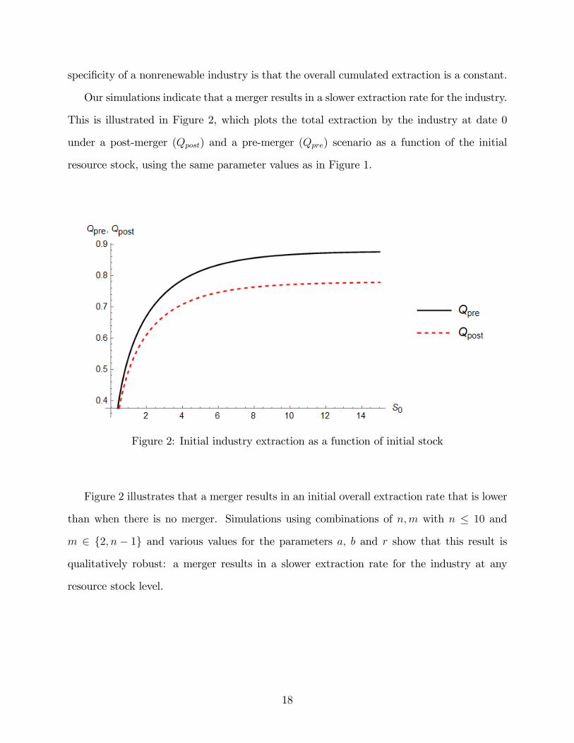
specificity of a nonrenewable industry is that the overall cumulated extraction is a constant.

Our simulations indicate that a merger results in a slower extraction rate for the industry.

This is illustrated in Figure 2, which plots the total extraction by the industry at date 0

under a post-merger (Qpost) and a pre-merger (Qpre) scenario as a function of the initial

resource stock, using the same parameter values as in Figure 1.

Figure 2: Initial industry extraction as a function of initial stock

Figure 2 illustrates that a merger results in an initial overall extraction rate that is lower

than when there is no merger. Simulations using combinations of n,m with n ≤ 10 and

m ∈ 2, n− 1 and various values for the parameters a, b and r show that this result is

qualitatively robust: a merger results in a slower extraction rate for the industry at any

resource stock level.

18

3.3 The case of an asymmetric oligopoly

We now use a numerical experiment to illustrate that Proposition 2 carries over when firms

have different initial endowments of the resource. Consider three firms, two with an initial

stock S0L and one with an initial stock S0S = fS0L, where f ∈ (0, 1]. Figure 3 illustrates, as

a function of S0L, the gains resulting from a merger of the two firms with initial stock S0L,

using the same parameter values as in Figures 1 and 2. In line with Proposition 2, Figure 3

shows that the merger is profitable when the value of S0L is suffi ciently small.

Figure 3: Gains from merger as a function of S0L

The following result is robust to changes in parameter values.

Result 1: A given merger is more likely to be profitable the smaller is the stock of the

outsider and the larger are the stocks of the merger participants.

Result 1 is illustrated in Figure 3, where the smaller is f , the greater is the range of S0L

for which the merger is profitable. This may explain why some of the largest firms in the

oil extraction sector have merged since the 1990’s. This result is intuitive: we know that a

merger of two firms in a duopoly is always profitable. The smaller the outsider firm’s stock

relative to the stock of the merged firms when two firms merge, the closer the profit of the

19

merged firm to the profit of a merger of firms in a duopoly. Therefore, a merger of two firms

in the case of a triopoly, when the outsider firm’s stock is small relative to the stock of the

merged firms, is more likely to be profitable than when the outsider firm’s stock is large

relative to the stock of the merged firms.

4 Impact of a tax on extraction

Non renewable resource industries can be important sources of pollution. A natural policy

instrument that is often considered is the imposition of a unit tax on the resource produced.

In this section, we examine the interplay of such policy on firms’incentives to merge and,

thus, on the industry’s market structure.

More precisely, we examine the effect of stricter environmental policies where, for sim-

plicity, we assume that each unit extracted generates a unit of polluting emissions. The

policy maker sets a constant tax per unit of extraction, τ . The objective function of a firm

i is then given by:

maxqi

∫ ∞0

e−rt [a− b (QS (t) +QL (t))− c− τ ] qi (t) dt (30)

subject to the resource constraint. The OLNE and the profitability analysis can then be

directly exploited by assuming that the marginal cost of extraction is increased by τ . Our

numerical simulations yield the following result, which is robust to changes in the parameter

values.

Result 2: A given merger is less likely to be profitable the higher the emission tax.

Result 2 is illustrated by Figure 4, where the higher is τ , the smaller is the range of S0L

for which the merger is profitable.

20

Figure 4: Gains from merger as a function of S0L with f = 0.5

An implication of Result 2 is that the emission of pollutants may be affected in a perverse

manner due to the imposition of a higher emission tax, resulting in a green paradox. Note

that in Hotelling models in which the long-run cumulative extraction is not impacted by the

tax, a constant unit tax induces markets to postpone the extraction of the resource. Indeed,

a constant tax means that the present value of the tax decreases over time, encouraging

markets to delay extraction, irrespective of the market structure. Thus, the first effect of the

tax policy under study is opposite to a green paradox. On the other hand, Result 2 indicates

that a tax might deter a merger, which increases the speed of extraction. This is the second

effect, which drives the green paradox. In what follows, we illustrate that, when a merger is

deterred due to a higher emission tax, the second effect dominates within our context.

Indeed, as noted in Section 3.2, a merger results in a lower initial extraction rate of the

resource than in the premerger scenario. If an increase in τ prevents a merger from being

realized that would otherwise have occured, the path of emissions in equilibrium is altered,

so that more emissions occur earlier than would have been the case with a lower tax level.

This is illustrated with the following example of a symmetric triopoly where we set again

a = 0.8555, b = 0.85552, r = 0.1 and examine the impact of a unit tax τ = 0.05. Figure

21

5 plots the industry’s initial extraction rate as a function of the stock in four cases: (i)

symmetric triopoly (Qpre) and τ = 0, (ii) symmetric triopoly and τ = 0.05, (iii) merger of

2 firms among 3 (Qpost) and τ = 0 and (iv) merger of 2 firms among 3 and τ = 0.05. We

note again that, for both τ = 0 and τ = 0.05, a merger results in a decrease of the initial

industry’s extraction rate, for all initial stock levels.

To illustrate the implication of Result 2, we consider the case where S0 = S0L = S0S = 7.5.

The gains from a merger when τ = 0 (resp. τ = 0.05) are 0.0154 (resp. −0.0006). That is, a

merger is profitable when τ = 0 and unprofitable when τ = 0.05. Comparing the extraction

rates under case (ii) and case (iii), we find from Figure 5 that the industry’s extraction rate

are higher under case (ii) than under case (iii). Figure 6 plots the path of the industry’s

cumulative extraction rate under case (ii) and case (iii): when the profitability of a merger

is taken into account, a tax of τ = 0.05 results in a faster depletion of the resource than the

case of τ = 0.

Figure 5: Initial industry extraction as a function of initial stock

22

Figure 6: Industry extraction path

In cases where the damage from pollution, which we have not explicitly modeled in this

paper, is convex in the emission level and/or where pollution is accumulative, the prevention

of the merger due to a higher tax could ultimately adversely affect the environment.

5 The case of economic exhaustion

Thus far, we have assumed the physical exhaustion of the resource. For some resources, the

marginal extraction cost is a decreasing function of the level of the stock. In this case, it

may happen that the extraction cost increases to levels that render the exploitation of the

remaining stock unprofitable, so that some resource is left in the ground. We now revisit the

profitability of a merger in an oligopolistic industry in this case.

Assume that the marginal cost of extraction from each mine8 is given by:

c0 − c1S,8We use the term "mine" to represent more generally a single facility from which the resource is ex-

tracted.

23

where c0 > 0 and c1 > 0 are such that the choke price a < c0, which implies that a mine will

be shut down when the stock reaches the level

S ≡ c0 − ac1

.

For comparison purposes, we limit our attention to the case of a symmetric triopoly where

each firm owns an initial stock S0, with S0 > S. Let x ≡ S − S, it is straightfoward to

rewrite the discounted sum of profits of firm i = 1, 2, 3 as

∫ ∞0

(−bQ+ c1xi) qie−rtdt. (31)

Firm i maximizes (31) subject to

xi = −qi (32)

and

xi (0) = x0 ≡ S0 − S. (33)

Proposition 3: Let

q (t) = −σeσtx0 (34)

where

σ ≡ 1

2

(r −

√r(c1 + r)

)< 0,

then the vector (q, q, q) constitutes an OLNE of the symmetric triopoly game.

Proof: See Appendix.

From Proposition 3, it follows that the equilibrium discounted sum of profits of a single

firm is given by:

∫ ∞0

− (3bσx+ c1x)σxe−rtdt = −x20 (3bσ + c1)σ

∫ ∞0

e−(−2σ+r)tdt

= −σ3bσ + c1−2σ + r

x20.

24

We now consider a merger of 2 firms. Since the marginal cost of extraction is no longer

constant, we can no longer use the pre-merger equilibrium to deduce the post-merger equi-

librium. Consider an industry that consists of two firms, an outsider firm that owns a single

mine and a merged entity that owns two mines, mine 1 and mine 2. Let SS (·), SL1 (·) and

SL2 (·) respectively denote the stock path of the outsider firm and of mine 1 and mine 2 of

the merged entity with SS (0) = S0S, SL1 (0) = S0L1 and SL2 (0) = S0L2. Denote by qS (·)

the extraction path of the outsider firm and by qL1 (·) and qL2 (·) the extraction paths of

the merged entity from mine 1 and mine 2 respectively. We drop the argument of the paths

whenever the explicit reference to time is not necessary. While the outsider firm chooses qS,

the merged entity chooses a pair of extraction paths qL1, qL2.

Proposition 4: Suppose that S0S = S0L1 = S0L2 = S0 and let x0 = S0− S, then the vector

(qo, qm, qm) where

qo (t) = −1

6((3 +

√3)µ1e

µ1t − (−3 +√

3)µ3eµ3t)x0 (35)

and

qm (t) =1

6(−(3 + 2

√3)µ1e

µ1t + (−3 + 2√

3)µ3eµ3t)x0 (36)

with

µ1 =1

2r − 1

2

√1

3br(

6c1 − 2√

3c1 + 3br)< 0 (37)

and

µ3 =1

2r − 1

2

√1

3br(

6c1 + 2√

3c1 + 3br)< 0 (38)

constitutes an OLNE between the merged entity and the outsider firm.

Proof: See Appendix.

It is now straightforward, using Propositions 3 and 4, to compute the equilibrium dis-

counted sum of profits for each firm under both the pre-merger scenario and when a merger

occurs, from which we can then infer the profitability of a merger. Let Wol (x0) denote the

25

equilibrium discounted sum of profits of a merged entity and Vol (x0) denote the equilibrium

discounted sum of profits for the two firms that merge under the pre-merger scenario, when

all firms own identical stocks x0. It can be shown that

Vol (x0) = 2σ (c1 + 3σ)

2σ − r x20

and that

Wol (x0) = −1

6

(Ωc1 −

(19 + 11

√3)µ21

2µ1 − r+

(−19 + 11

√3)µ23

2d3 − r+

2µ1µ3µ1 + µ3 − r

)x20

where

Ω ≡ µ1

(− 7

(2µ1 − r)− 4

√3

(2µ1 − r)+

1

µ1 + µ3 − r

)

+µ3

(− 7

(2µ3 − r)+

4√

3

(2µ3 − r)+

1

µ1 + µ3 − r

).

Result 3: A merger of two firms can be profitable.

Result 3 is illustrated in Figure 7 using a numerical example, where we set r = 0.05, b = 1

and x0 = 100, and plot the gains from a merger Wol (x0)− Vol (x0) as a function of c1.

26

Gainsfrom merger

c1

Figure 7: Gains from a merger as a function of c1

We highlight two important qualitative differences with respect to the case of physical

scarcity: (i) when the firms’initial stocks are identical, whether a merger is profitable or not

does not depend on the initial stock level, (ii) when positive, the gains from a merger are

typically relatively very small.

Figure 8 illustrates how the relative gains from a merger, i.e. Wol(x0)−Vol(x0)Vol(x0)

, depend on

the parameter c1. The maximum gain from a merger is approximately 0.3% of the total

payoff when there is no merger. The larger is c1, the more important is the role of the cost

effect in the firm’s payoffs, and the less important is the market interaction between firms.

In this case, the extraction and payoff of a firm when a given merger occurs and when it

does not occur are very close to each other.

27

Relative Gainsfrom merger

c1

Figure 8: Relative gains from a merger as a function of c1

When c1 is suffi ciently small, then the market interaction is relatively more important

than the stock effect on costs, so that we retrieve the standard result from static oligopoly

theory that a merger of two firms is not profitable. These qualitive results are robust to

changes in the values of the parameters b and r.

6 Conclusion

This paper showed that, if resource stock levels are small enough, small mergers (mergers of

two firms) are profitable under constant marginal costs and may also be profitable when the

marginal cost is decreasing in the resource stock level. The profitability of mergers arises

because outsiders are limited in their response in terms of increased output due to their finite

resource stocks. Mergers allow the merger participants to raise prices more than in industries

without stock constraints. Therefore, antitrust authorities should be cautious when ruling on

mergers in non-renewable resource industries. At the same time, mergers in these industries

reduce environmental damage by delaying extraction.

The interplay of environmental regulations and incentives to merge deliver interesting

insights: an environmental tax can affect merger profitability. In the case of a polluting

28

resource, a unit tax on extraction may deter mergers and, therefore, may result in causing

emissions earlier than under laissez-faire. A small increase of the tax may result in a non-

marginal jump upwards of the industry’s pollution.

In our analysis, we ignored the possibility that a perfect substitute to the resource may

exist. This simplifies the analysis and, at the same time, allows to directly contrast our results

with those obtained in the SSR framework. However, e.g. for fossil fuels, the existence of

a backstop technology that can provide a substitute to the resource at a given fixed price,

and that is supplied by a perfectly competitive market, has received a significant amount of

attention. In this case, the resource owner, e.g., OPEC, can resort to limit pricing: charging a

price that is just enough to undercut the backstop substitute. Recent important contributions

on limit pricing arising in fossil fuel extraction include Andrade de Sa and Daubane (2016)

and Van der Meijden, Ryszka and Withagen (2018)9, or Salant (1977) and Hoel (1978, 1984)

for earlier contributions. A natural and relevant follow-up research question to our analysis is

the profitability of a merger or of cartel formation10 in the presence of a backstop substitute.

In that case, if, for example, initial endowments of the nonrenewable resource and/or demand

elasticity are such that limit pricing takes place from the initial date until the extinction of

the resource, then a merger may not affect the price path of the resource11 and a specific

analysis of cartel or merger profitability is in order. This is left for future research.

9Andrade de Sa and Daubane (2016) considers a nonrenewable resource monopoly facing a backstopsubstitute. They show that, when the price elasticity of demand is smaller than one, the monopolistchoses, at each moment, a corner solution, i.e., induces the limit price which deters the backstop-substituteproduction. Van der Meijden, Ryszka and Withagen (2018) consider a non-renewable resource supplierwho faces demand from two regions, one of which employs a tax on the imported resource and a subsidyon the available backstop technology, and one that has no environmental policy in place. They show thatthe resource extraction path possibly contains two limit pricing phases.10As noted above, in instances where resource owners are countries and not firms, coordination of inter-

ests among the resource owners takes the form of cartels rather than mergers.11We thank an anonymous referee for pointing to this possibility.

29

References

[1] Andrade de Sá, S. and J. Daubanes (2016). "Limit pricing and the (in) effectiveness of

the carbon tax," Journal of Public Economics, 139: 28-39.

[2] Benchekroun, H. & G. Gaudet (2003). “On the profitability of production perturbations

in a dynamic natural resource oligopoly,”Journal of Economic Dynamics and Control,

27(7): 1237-1252.

[3] Benchekroun, H. & G. Gaudet (2015). "On the effects of mergers on equilibrium out-

comes in a common property renewable asset oligopoly," Journal of Economic Dynamics

and Control, 52: 209-223.

[4] Benchekroun, H., A. Halsema & C. Withagen (2009). “On nonrenewable resource

oligopolies: the asymmetric case,” Journal of Economic Dynamics and Control, 33:

1867-1879.

[5] Benchekroun, H., A. Halsema & C. Withagen (2010). “When additional resource stocks

reduce welfare,”Journal of Environmental Economics and Management, 59: 109-114.

[6] Benchekroun H. & N.V. Long (2006). “The curse of windfall gains in a non renewable

resource oligopoly,”Australian Economic Papers, 45(2): 99-105.

[7] Colombo, L., & P. Labrecciosa (2015). “On the Markovian effi ciency of Bertrand and

Cournot equilibria,”Journal of Economic Theory, 155: 332—358.

[8] Dockner, E. J., S. Jorgensen, N.V. Long & G. Sorger (2000) “Differential games in

economics and management science," Cambridge University Press.

[9] Eswaran, M. & T. Lewis (1985). “Exhaustible resources and alternative equilibrium

concepts,”Canadian Journal of Economics, 18(3): 459-73.

[10] Farrell, J. & C. Shapiro (1990). “Horizontal mergers: an equilibrium analysis,”American

Economic Review, 80(1): 107-26.

30

[11] Gaudet, G. & N.V. Long (1994). “On the effects of the distribution of initial endow-

ments in a nonrenewable resource duopoly,”Journal of Economic Dynamics and Con-

trol, 18(6): 1189-1198.

[12] Gaudet, G. & S.W. Salant (1991). “Increasing the profits of a subset of firms in oligopoly

models with strategic substitutes,”American Economic Review, 81(3): 658-65.

[13] Groot, F., C. Withagen & A. de Zeeuw (1992). “Note on the open-loop von Stackelberg

equilibrium in the cartel versus fringe model,”Economic Journal, 102(415): 1478-84.

[14] Groot, F., C. Withagen & A. de Zeeuw (2003). “Strong time-consistency in the cartel-

versus-fringe model,”Journal of Economic Dynamics and Control, 28(2): 287-306.

[15] Hartwick, J. M. & M. Brolley (2008). “The quadratic oil extraction oligopoly,”Resource

and Energy Economics, 30(4): 568-577.

[16] Hoel, M. (1978). "Resource extraction, substitute production, and monopoly,". Journal

of Economic Theory, 19: 28—37.

[17] Hoel, M. (1984). "Extraction of a resource with a substitute for some of its uses,"

Canadian Journal of Economics, 17: 593—602.

[18] Kagan, M., van der Ploeg, F. and C. Withagen (2015). "Battle for climate and scarcity

rents: beyond the linear-quadratic case," Dynamic games and applications, 5(4): 493-

522.

[19] Kamien, M.I. & I. Zang (1990). “The limits of monopolization through acquisition,”

The Quarterly Journal of Economics, 105: 465-99.

[20] Kamien, M.I. & I. Zang (1991). “Competitively cost advantageous mergers and monop-

olization,”Games and Economic Behaviour, 3: 323-38.

[21] Kamien, M.I. & I. Zang (1993). “Monopolization by sequential acquisition,”Journal of

Law, Economics and Organization, 9(2): 205-29.

31

[22] Karp, L. & D. Newbery (1991). “OPEC and the U.S. oil import tariff,” Economic

Journal, 101(405): 303-13.

[23] Kumar, B.R. (2012). Mega Merger and Acquisitions: Case Studies from Key Industries.

Palgrave Macmillan.

[24] Lewis, T. R. and R. Schmalensee (1980). “On oligopolistic markets for nonrenewable

natural resources,”The Quarterly Journal of Economics, 95(3): 475-91.

[25] Long, N.V. (2015). “The Green Paradox in open economies: Lessons from static and

dynamic Models,”Review of Environmental Economics and Policy, 9(2): 266-284.

[26] Loury, G. C. (1986). “A theory of ‘Oil’igopoly: Cournot equilibrium in exhaustible

eesource markets with fixed supplies,”International Economic Review, 27(2): 285-301.

[27] van der Meijden, G., K. Ryszka and C. Withagen (2018). "Double limit pricing," Journal

of Environmental Economics and Management, 89: 153-167.

[28] Perry, M. K., & R.H. Porter (1985). "Oligopoly and the incentive for horizontal merger,"

American Economic Review, 75(1): 219-227.

[29] Pittel, K., R. van der Ploeg & C. Withagen (2014). Climate Policy and Nonrenewable

Resources: The Green Paradox and Beyond. MIT Press.

[30] Polasky, S. (1996). “Exploration and extraction in a duopoly-exhaustible resource mar-

ket,”Canadian Journal of Economics, 29(2): 473-492.

[31] Reinganum, J. F. & N. L. Stokey (1985). “Oligopoly extraction of a common property

natural resource: The importance of the period of commitment in Dynamic Games,”

International Economic Review, 26(1): 161-73.

[32] Salant, S. (1976). “Exhaustible resources and industrial structure: A Nash-Cournot

approach to the world oil market”, Journal of Political Economy, 84: 1079-1093.

32

[33] Salant, S. (1977). "Staving off the backstop: dynamic limit-pricing with a kinked de-

mand curve," Board of Governors of the Federal Reserve System (U.S.), International

Finance Discussion Papers 110.

[34] Salant, S. (1982). “Imperfect competition in the international energy market,”Opera-

tions Research, 2: 252-280.

[35] Salant, S.W., S. Switzer & R.J. Reynolds (1983). “Losses from horizontal merger: The

effects of an exogenous change in industry structure on Cournot-Nash equilibrium,”

Quarterly Journal of Economics, 98: 185-199.

[36] Salo, S. & O. Tahvonen (2001). “Oligopoly equilibria in nonrenewable resource markets,”

Journal of Economic Dynamics and Control, 25: 671-702.

[37] Sinn, H. W. (2008). “Public policies against global warming: a supply side approach,”

International Tax and Public Finance, 15(4): 360-394.

[38] Stigler, G.J.(1950). “Monopoly and oligopoly by merger,” The American Economic

Review, 40: 23-34.

[39] Wan, R.& J. Boyce (2014). “Non-renewable resource Stackelberg games,”Resource and

Energy Economics, 37: 102-121.

33

Appendix:

Proof of Proposition 3

Consider the symmetric triopoly game described by (31-33), given extraction paths q1 and

q2 of firm 1 and firm 2; the necessary conditions for a positive extraction q3 of the third firm

are given by

Hq3 = −2bq3 − q1 − q2 + c1x− λ3 = 0 (39)

λ3 = rλ3 − c1q3 (40)

x = −q3 (41)

x (0) = x0

with

limt→∞

x (t) = 0

For a symmetric equilibrium and interior solutions, we have q3 = q1 = q2 = q, and

λ3 = λ1 = λ2 = λ. From (39) , we obtain the following:

λ = −4bq + c1x

and therefore

λ = −4bq + c1x. (42)

From (40) and (42), we obtain:

−4bq + c1x = r (−4bq + c1x)− c1q (43)

From (41) and (43) , it follows that the symmetric OLNE when firms are identical is given

34

by the solution to the following system:

q = rq − c14brx (44)

x = −q (45)

x (0) = x0

with

limt→∞

x (t) = 0.

Moreover, (44) and (45) , yield:

q

x

=

r − rc14b

−1 0

qS

x

.

The two eigenvalues of

r − rc14b

−1 0

are given by σ1 = 12

(r −

√1b

(br2 + c1r))< 0 and

σ2 = 12

(r +

√1br (c1 + br)

)> 0, and the associated eigenvectors are

−σ11

and

−σ21

respectively.

Given that the trajectory cannot oscillate around the steady state, the solution is given

by: q

x

= A

σeσt

eσt

with A = x0 and σ = σ1.

Therefore, the OLNE path is given by:

q

x

= x0

−σeσteσt

35

Proof of Proposition 4

The merged entity, denoted firm M , controls two stocks, denoted SL1 and SL2 :

SL1 = −qL1

SL2 = −qL2

where qLi is the extraction from stock SLi with i = 1, 2. Firm M maximizes the joint profit

from both stocks and the outsider controls stock SS. We therefore have the following:

HS (qS, λS, t) = [a− b (QS +QL)− c0 + c1SS] qS + λS (−qS) .

HM (qL1, qL2, λL1, λL2, t) = [a− b (QS +QL)− c0 + c1SL1] qL1

+ [a− b (QS +QL)− c0 + c1SL2] qL2

+λL1 (−qL1) + λL2 (−qL2) .

The maximum principle yields

HSqS

= a− c0 − 2bqS − bQL + c1SS − λS (46)

HMqL1

= a− c0 − 2bqL1 − 2bqL2 − bqS + c1SL1 − λL1 (47)

HMqL2

= a− c0 − 2bqL2 − 2bqL1 − bqS + c1SL2 − λL2 (48)

where Hz denotes the partial derivative of H with respect to variable z.

The necessary conditions are

HSqS≤ 0 and HS

qSqS = 0

36

HMqL1≤ 0 and HM

qL1qL1 = 0

HMqL2≤ 0 and HM

qL2qL2 = 0

The other Maximum Principle conditions are

λS = rλS − c1qS

λL1 = rλL1 − c1qL1

λL2 = rλL2 − c1qL2

and

SS = −qS

SL1 = −qL1

SL2 = −qL2

with

SS (0) = S0S

SL1 (0) = S0L1

SL2 (0) = S0L2

When S0L1 = S0L2 = S0, the Merged entity operates both mines at qL1 = qL2 and,

therefore,

HSqS

= −2bqS − bQL + c1SS − λS (49)

HMqL1

= −4bqL1 − bqS + c1SL1 − λL1. (50)

The necessary conditions are

HSqS≤ 0 and HS

qSqS = 0

37

HMqL1≤ 0 and HM

qL1qL1 = 0.

The other Maximum Principle conditions are

λS = rλS − c1qS

λL1 = rλL1 − c1qL1

and

SS = −qS

SL1 = −qL1,

with

SS (0) = S0S

SL1 (0) = S0L1.

Three different regimes can occur: Simultaneous(ΦS), Merged entity produces alone (ΦM),

and Outsider produces alone (ΦO). We focus on the regime where the solution is interior,

i.e. regime ΦS :

−2bqS − 2bqL1 + c1SS = λS (51)

−4bqL1 − bqS + c1SL1 = λL1. (52)

Taking the time derivative of the conditions above yields

−2bqS − 2bqL1 + c1SS = λS (53)

−4bqL1 − bqS + c1SL1 = λL1, (54)

38

and, therefore, the other Maximum Principle conditions yield

−2bqS − 2bqL1 + c1SS = r (−2bqS − 2bqL1 + c1SS)− c1qS

−4bqL1 − bqS + c1SL1 = r (−4bqL1 − bqS + c1SL1)− c1qL1

or

−2bqS − 2bqL1 = r (−2bqS − 2bqL1 + c1SS) (55)

−4bqL1 − bqS = r (−4bqL1 − bqS + c1SL1) (56)

and

SS = −qS

SL1 = −qL1,

with

SS (0) = S0S

SL1 (0) = S0L1,

along with

limt→∞

SS (t) =c0 − ac1

and limt→∞

SL1 (t) =c0 − ac1

.

From (55) and (56) , we obtain

−4bqS − 4bqL1 = 2r (−2bqS − 2bqL1 + c1SS)

−4bqL1 − bqS = r (−4bqL1 − bqS + c1SL1) .

Therefore

−3bqS = 2r (−2bqS − 2bqL1 + c1SS)− r (−4bqL1 − bqS + c1SL1)

39

6bqL1 = −2r (−4bqL1 − bqS + c1SL1) + r (−2bqS − 2bqL1 + c1SS)

or

−3bqS = r (−3bqS + 2c1SS − c1SL1)

6bqL1 = r (6bqL1 − 2c1SL1 + c1SS) .

Equivalently

qS = rqS − r2c13bSS + r

c13bSL1 (57)

qL1 = rqL1 − r2c16bSL1 + r

c16bSS (58)

with

SS = −qS (59)

SL1 = −qL1, (60)

and the initial and transversality conditions

SS (0) = S0S (61)

SL1 (0) = S0L1 (62)

limt→∞

SS (t) = 0 and limt→∞

SL1 (t) = 0. (63)

Solving the system of differential equation (57) − (60) with the conditions (61) − (63)

yields (35) and (36)

40