techno-economic analysis and benchmarking of … resource recovery technologies for wastewater...
TRANSCRIPT
Techno-economic Analysis and Benchmarking
of Resource Recovery Technologies for
Wastewater Treatment Plants
Beatriz Ferreira Matafome
Thesis to obtain the Master of Science Degree in
Biological Engineering
Supervisors: Professor Ana Isabel Cerqueira de Sousa Gouveia Carvalho
Professor Gürkan Sin
Examination Committee
Chairperson: Duarte Miguel de França Teixeira dos Prazeres
Supervisor: Professor Ana Isabel Cerqueira de Sousa Gouveia Carvalho
Member of the Committee: Professor Helena Maria Rodrigues Vasconcelos Pinheiro
October 2016

ii
[This page was intentionally left blank]
iii
ACKNOWLEDGEMENTS
Firstly, I would like to address my sincerest gratitude to Professor Gürkan Sin for allowing me
to work under his guidance at CAPEC-PROCESS Centre at Technical University of Denmark (DTU)
and accompanying me during the development of my master dissertation. It was a very stimulant and
challenging project that gave me the opportunity to further develop my knowledge either on the
academic and personal level.
Secondly, I am very grateful for my supervisor at Instituto Superior Técnico (IST), Professor
Ana Carvalho, for all the support and guidance, especially in the beginning of my exchange process at
DTU, but also for her contribution to the improvement of my thesis.
A special thank you to Carina Gargalo, from DTU, for believing in me since the first moment
and giving me the opportunity to work on this project and for all the support and advices throughout the
entire process. To Riccardo Boiocchi, thank you so much for all the learning process and the constant
support, for never letting me quit and always believing in me.
For all the CAPEC-PROCESS Centre I thank you for so kindly receiving me and for being so
helpful all the times.
For all the people that guided me through my academic life and allowed me to get to the point
where I stand today, thank you so much.
To my friends, the ‘Fitsches’, the ‘Piranhas’ and the ‘AAA’, who I would not be the same without,
I would like to thank for always lightening my days and for all the encouragement and motivation, even
so far apart. To Guilherme thank you for always believing in me and never letting me give up on my
objectives. To Rita, a special thank you for always listening to me and for including me in your life as if
I was part of your family. To Duarte thank you for the amazing life experience and for always getting my
head out of the problems.
Finally, I would like to give a special appreciation to my parents, António Pedro and Maria de
Lurdes, to my grandparents Judite, Joaquim and Maria Helena, to my aunt and godmother Helena
Teresa, to my uncle Carlos, to my cousins Ana Rita, António Miguel, Catarina, Francisco, Maria Inês
and Miguel Bento for your love and for the endless support in all the important moments of my life.

iv
[This page was intentionally left blank]

v
ABSTRACT
The growth of the world population and spread of industrialization have put a relentless pressure
on resources. Wastewater treatment plants are large resource consumers and are now perceived as a
promising effort to detain the global resources crisis through sustainable action. Therefore, the present
work focusses on retrofitting a WWTP through resource recovery, aiming to reduce the operating costs
of the plant.
To this end, the Benchmark Simulation Model No. 2 (BSM2) is used as the starting setting of a
WWTP and is extended in order to include the following full-scale technologies for recovery of added-
value products: a) the chemical precipitation process, for recovery of iron phosphate (FePO4) fertilizer;
b) the Exelys technology, for increased biogas production; and c) the Phosnix technology, for recovery
of struvite (MgNH4PO4.6H2O) fertilizer. The technologies are added to the BSM2 layout according to
different combinations, generating 7 distinct simulation scenarios.
Global mass balances to the phosphorus and nitrogen components were performed to evaluate
the feasibility of the extended benchmark simulation models, along with an economic evaluation in order
to identify the most profitable retrofitted scenario. A sensitivity analysis was performed, as well, to
quantify the impact of the introduction of the resource recovery units into the BSM2 plant.
It was concluded that the most economically feasible scenario includes solely the addition of the
Phosnix technology to the BSM2, for struvite precipitation, with an operating profit of 87,32 k€/year.
Keywords: Wastewater treatment, Benchmark Simulation Model No. 2, retrofit, resource recovery.

vi
[This page was intentionally left blank]

vii
RESUMO
O crescimento da população mundial e expansão da industrialização resultam numa pressão
implacável sobre os recursos terrestres. As estações de tratamento de águas (ETARs) são grandes
consumidores de recursos, sendo vistos presentemente como um esforço promissor para deter a crise
global de recursos através de uma ação sustentável. Assim, o presente trabalho foca-se no “retrofitting”
de uma ETAR através da recuperação de recursos, com o objetivo de diminuir os custos operacionais
da planta.
Para isso, o modelo “Benchmark Simulation Model Nº 2” (BSM2) foi usado como configuração
inicial de uma ETAR e foi alargado para incluir as seguintes tecnologias de larga escala para
recuperação de produtos de valor acrescentado: a) precipitação química, para recuperar um fertilizante
de fosfato de ferro (FePO4); b) a tecnologia Exelys, para aumentar a produção de biogás; e c) a
tecnologia Phosnix, para recuperar estruvite (MgNH4PO4.6H2O-fertilizante). As tecnologias são
acrescentadas ao BSM2 em combinações diferentes, criando 7 cenários de simulação distintos.
Foram efetuados balanços de massa globais aos componentes fósforo e nitrogénio para avaliar
a viabilidade dos modelos de simulação estudados, assim como uma avaliação económica para
identificar qual o cenário “retrofitted” mais lucrativo. Foi ainda realizada uma análise de sensibilidades
para quantificar o impacto da introdução das unidades para recuperação de recursos no modelo BSM2.
Concluiu-se que o cenário de simulação economicamente mais viável corresponde apenas à
introdução da tecnologia Phosnix no BSM2, apresentando um lucro operacional de 87,32 k€ por ano.
Palavras-chave: Tratamento de águas, “Benchmark Simulation Model No. 2”, “retrofit”, recuperação
de recursos.

viii
[This page was intentionally left blank]

ix
TABLE OF CONTENTS
ACKNOWLEDGEMENTS ................................................................................................................................ III
ABSTRACT ...........................................................................................................................................................V
RESUMO ........................................................................................................................................................... VII
TABLE OF CONTENTS .................................................................................................................................... IX
LIST OF FIGURES ............................................................................................................................................XII
LIST OF TABLES ........................................................................................................................................... XIII
LIST OF ABBREVIATIONS .............................................................................................................................. 1
1 INTRODUCTION ........................................................................................................................................ 4
1.1 CONTEXT ................................................................................................................................................................ 4
1.2 OBJECTIVE ............................................................................................................................................................. 4
1.3 METHODOLOGY..................................................................................................................................................... 5
1.4 OUTLINE OF THE THESIS ..................................................................................................................................... 5
2 LITERATURE REVIEW ............................................................................................................................. 7
2.1 WASTEWATER TREATMENT DEVELOPMENT .................................................................................................. 7
2.2 RESOURCE RECOVERY FROM WWTP ............................................................................................................... 9
2.2.1 Onsite Energy Generation ............................................................................................................................ 9
2.2.2 Nutrient Recovery .........................................................................................................................................12
2.3 MODELLING OF WASTEWATER TREATMENT SYSTEMS ............................................................................... 17
2.3.1 ASM1 - Activated Sludge Model Number 1 ........................................................................................17
2.3.2 Other Activated Sludge Models – ASM2, ASM2d, ASM3 ...............................................................19
2.3.3 Benchmark Simulation Models ...............................................................................................................20

x
2.3.4 ADM1 – Anaerobic Digestion Model No. 1 .........................................................................................23
2.4 CHAPTER CONCLUSIONS ................................................................................................................................... 23
3 MODEL DEVELOPMENT ....................................................................................................................... 24
3.1 BENCHMARK SIMULATION MODEL NO. 2 OVERVIEW ................................................................................. 24
3.1.1 ASM1-Activated Sludge Unit.....................................................................................................................25
3.1.2 Anaerobic Digestion Process Model ......................................................................................................29
3.2 APPLICATION OF DIFFERENT SIMULATION SCENARIOS .............................................................................. 33
3.3 MATHEMATICAL FORMULATION AND MODEL ASSUMPTIONS .................................................................... 35
3.3.1 Introduction of the Chemical Precipitation Technology into the BSM2 ..............................35
3.3.2 Introduction of the Exelys Technology into BSM2 .........................................................................36
3.3.3 Introduction of the Phosnix Technology into BSM2 ......................................................................38
3.4 DATA ANALYSIS .................................................................................................................................................. 39
3.4.1 Global Mass Balance ....................................................................................................................................39
3.4.2 Economic Evaluation ...................................................................................................................................39
3.5 CHAPTER CONCLUSIONS ................................................................................................................................... 48
4 RESULTS AND DISCUSSION ................................................................................................................ 49
4.1 GLOBAL MASS BALANCE RESULTS .................................................................................................................. 49
4.2 ECONOMIC EVALUATION RESULTS .................................................................................................................. 50
4.2.1 Operating Costs ..............................................................................................................................................50
4.2.2 Revenue and Operating profit .................................................................................................................63
4.3 CHAPTER CONCLUSIONS ................................................................................................................................... 65
5 SENSITIVITY ANALYSIS ....................................................................................................................... 66

xi
5.1 UNCERTAINTY INPUTS SELECTION, FRAMING AND SAMPLING .................................................................. 66
5.2 MONTE-CARLO SIMULATION ........................................................................................................................... 68
5.3 LINEAR REGRESSION OF MONTE-CARLO SIMULATIONS.............................................................................. 68
5.4 SENSITIVITY ANALYSIS RESULTS ..................................................................................................................... 68
5.5 INTERPRETATIONS OF SENSITIVITY ANALYSIS RESULTS ............................................................................ 69
5.6 CHAPTER CONCLUSIONS ................................................................................................................................... 73
6 CONCLUSION AND FUTURE REMARKS ........................................................................................... 75
7 REFERENCES ........................................................................................................................................... 77
8 APPENDIX ................................................................................................................................................ 82
8.1 ASM1 ................................................................................................................................................................... 82
8.1.1 Biological Processes .....................................................................................................................................82
8.1.2 Settling Process ..............................................................................................................................................82
8.2 ADM1 .................................................................................................................................................................. 83
8.3 MATLAB/SIMULINK IMPLEMENTED FUNCTIONS ......................................................................................... 85
8.3.1 Chemical Precipitation ................................................................................................................................85
8.3.2 Exelys Technology .........................................................................................................................................86
8.3.3 Phosnix Technology ......................................................................................................................................88
8.4 MATLAB/SIMULINK SIMULATION RESULTS .................................................................................................. 89
8.4.1 Global Mass Balances...................................................................................................................................89
8.4.2 Economic Evaluation ...................................................................................................................................93

xii
LIST OF FIGURES
Figure 1 – Methodology followed in this thesis. ...................................................................................... 5
Figure 2 – Generalized flow process diagram for wastewater treatment [13]. ....................................... 8
Figure 3 - Typical configuration of thermal hydrolysis in a sludge treatment line [19]. ........................ 11
Figure 4 - Exelys process scheme [22]. ............................................................................................... 12
Figure 5 - The Crystalactor® fluidized bed reactor and the Crystalactor® reactors at the
Geestmerambacht WWTP [28]. ..................................................................................................... 13
Figure 6 - The AirPrex procedure [28], [32]. ......................................................................................... 14
Figure 7 – Schematic representation of the Ostara Pearl® process. [28] ............................................ 14
Figure 8 – Schematic representation of the Phosnix process in the WWTP. ....................................... 15
Figure 9 – Schematic representation of the Seaborne process in the WWTP. .................................... 15
Figure 10 – General overview of the BSM1 plant [37]. ......................................................................... 21
Figure 11 – General overview of the BSM2 plant [8]. ........................................................................... 22
Figure 12 - Schematic representation of the extended BSM2 layout including the three technologies
introduced into the BSM2. Each technology is enlighten with a different colour: the chemical
precipitation is represented in red, the thermal hydrolysis – Exelys technology - is represented in
green and the struvite precipitation unit – Phosnix technology - is represented in blue. The
technologies are generally represented. ....................................................................................... 33
Figure 13 – Superstructure representation of the resource recovery technologies implemented into
BSM2 (WW – wastewater, PC – primary clarifier, AS – activated sludge, CP – chemical
precipitation, T - thickener; AD – anaerobic digestion, DU - dewatering unit). The path enlighten in
grey represents the BSM2 base-case (scenario 0 – C0). The dewatering unit number 1 is included
in the Exelys technology. ............................................................................................................... 34
Figure 14 – Exelys process scheme [22]. ............................................................................................. 36
Figure 15 – Schematic representation of biomass degradation assumed for the Exelys technology.
Legend: interm-intermediate. ......................................................................................................... 37
Figure 16 – Schematic representation of the boundary established for the implementation of the global
mass balance. The boundary considered in represented in grey. ................................................. 49

xiii
LIST OF TABLES
Table 1 – Summary of the technologies and respective applications of onsite energy generation in
WWTPs [17]. .................................................................................................................................. 10
Table 2 – Summary of the technologies and respective applications for resource recovery in WWTPs
[28].................................................................................................................................................. 12
Table 3 – Summary of the full-scale technologies for resource-recovery. ............................................ 16
Table 4 – Summary of the existing ASMs for the activated sludge unit. Legend: Den. PAO (Denitrifying
PAO activity included in the model), DR (death regeneration concept), EA (electron acceptor
depending), ER (endogenous respiration concept), Cst (non-electron acceptor depending). The dot
symbol, • , identifies that a given process is present in a model [11]............................................. 17
Table 5 - Example of a simple stoichiometric matrix for activated sludge modelling (adapted from [11]).
........................................................................................................................................................ 19
Table 6 – Influent values considered in the BSM2. .............................................................................. 24
Table 7 – Operational conditions assumed in the BSM2. ..................................................................... 25
Table 8 – Summary of the main components in the BSM2 [38]. .......................................................... 25
Table 9 - State variables for the IAWQ Activated Sludge Model No. 1 (ASM1) [35]. ........................... 26
Table 10 - Rate equations for all processes included in ASM1 [35]. .................................................... 26
Table 11 - Matrix representation of ASM1 showing the processes, components, process rate equations,
and stoichiometry [35]. ................................................................................................................... 28
Table 12 - Definition of the symbols representing all the components of the model [46]. .................... 29
Table 13 - Rate equations for all processes included in ADM1 [46]. .................................................... 30
Table 14 - Biochemical rate coefficients (vi,j) and kinetic rate equations (ρj) for soluble components (i=1-
12, j=1-19) in the ADM1 model. Missing values are equal to 0. [46]. ............................................ 31
Table 15 - (Continuation of Table 14) Biochemical rate coefficients (vi,j) and kinetic rate equations (ρj)
for soluble components (i=1-12, j=1-19) in the ADM1 model. Missing values are equal to 0 [46]. 32
Table 16 – Simulation scenarios considered. ....................................................................................... 33

xiv
Table 17 – Summary of the required pieces of equipment for each technology introduced into BSM2
that require energy consumption. ................................................................................................... 43
Table 18 – Dosages and weighted average prices for the reactants and utilities introduced into the
BSM2 (pp – precipitated). .............................................................................................................. 47
Table 19 – Weighted commercial value (€/kg) assumed for each added-value product recovered in the
BSM2 plant. .................................................................................................................................... 48
Table 20 – Global mass balance for C0. The column denominated %influent (m/m) calculates the
percentage of each output component related to total nitrogen or phosphorus in the influent,
depending on the component in question. ..................................................................................... 50
Table 21 – Calculation of the pollutant loads for the effluent streams (TSS, COD, TKN, SNO, BOD5, EQI
(kg Pollution Units (PU)/(d))and calculation of the respective effluent quality costs (k€/y). ........... 51
Table 22 – Sludge production (kg/y) and sludge production associated costs (k€/y)........................... 52
Table 23 – External carbon source (kg/y) and associated costs (k€/y). ............................................... 53
Table 24 – Energy consumption for BSM2 base-case configuration (AE, PE, MEAS, MEAD, ME, EBase-
case) (kWh/y). ................................................................................................................................... 54
Table 25 - Equipment dimensions for each BSM2 scenario. ............................................................... 55
Table 26 – Power requirements (kWh/y) for the pieces of equipment present in each configuration of
BSM2. Legend: MixerE, FloccE, ExelysE, PhosnixE- equipment energy requirements for the mixer
and the flocculator (chemical precipitation), and for the Exelys and Phosnix technologies,
respectively. EBSM2 extended – overall equipment energy requirements for the resource recovery
technologies. .................................................................................................................................. 56
Table 27 – Total energy consumed by the equipment for the different simulation scenarios tested.
Legend: EBSM2 – equipment energy requirements from the reference BSM2 (are the same for every
scenario); EBSM2 extended – equipment energy requirements of the chemical precipitation, the Exelys
and the Phosnix technologies all together; Eequipment – is the sum of EBSM2 and EBSM2 extended (see
also equation (37)). ........................................................................................................................ 57
Table 28 – Energy recovered from the BSM2 plant (EHE, ECH4, ECH4 Steam and ECH4 Power (kWh/y)) and
energy consumed by the Exelys technology (Esteam (kWh/y)) for the different BSM2 configurations.
........................................................................................................................................................ 58
Table 29 – Energy consumed for production of the steam used in the Exelys technology. ................. 60

xv
Table 30 – Energy consumption required left by the BSM2 plant after the consumption of the renewable
plant and remaining renewable energy produced by the plant that was not consumed (kWh/y).
Energy (EN) costs (+) and/or savings/profit (-) for the different configurations of the BSM2 plant
(k€/y). ............................................................................................................................................. 61
Table 31 – Soluble phosphorus precipitated by the chemical precipitation (SPO4-P,pp-CP) and the Phosnix
technology (SPO4-P,pp-Phosnix) (kg PO43-/y). FeSO4.7H2O and Mg(OH)2 costs for each configuration
(k€/y). ............................................................................................................................................. 62
Table 32 – EQ, SP, EC, EN, RU and OC costs (k€/y) for each BSM2 combination considered. ......... 63
Table 33 – Chemical precipitation, Phosnix and revenues and operating profit for each BSM2
configuration (k€/y). ........................................................................................................................ 64
Table 34 – Uncertainty inputs mean values and framing intervals. Phosnix yield is the Phosnix
technology yield, CP yield is the chemical precipitation yield, % TSSsolubilized Exelys is the percentage
of TSS that is solubilized in the Exelys technology, [P]influent is the P concentration in the WWTP’s
influent (kg COD/m3), [SNH]influent is the ammonia/ammonium concentration in the influent (kg
COD/m3), [XS]influent is the suspended solids concentration in the influent (kg COD/m3), KI NH3 is the
free ammonia inhibition constant (dimensionless), Volume AD is the anaerobic digester’s volume
(m3), %TSSremoval, DU is the percentage of TSS removed in the dewatering unit after the anaerobic
digestion unit. ................................................................................................................................. 66
Table 35 – Outputs selected for the sensitivity analysis. Legend: AE is the aeration energy, PE is the
pumping energy, SP is the sludge production, ECH4 is the methane energy, kLa Tank 3 is the volumetric
oxygen transfer coefficient in activated sludge tank number 3, TSS Load Eff, COD Load Eff, TKN Load Eff,
SNO Load Eff and P Load Eff are the amount of TSS, COD, TKN, SNO and P in the effluent stream,
respectively. ................................................................................................................................... 69
Table 36 – Standardized regression coefficients, βi, coefficients of determination, R2, and relative
variance contributions, βi2, for each of the analysed outputs. ........................................................ 69
Table 37 - Stoichiometric parameter values for ASM1 in the ‘simulation benchmark’.......................... 82
Table 38 - Kinetic parameter values for ASM1 in the ‘simulation benchmark’. .................................... 82
Table 39 - Settler model parameters and default values. ..................................................................... 82
Table 40 - Stoichiometric parameter values for ADM1. ........................................................................ 83
Table 41 - Kinetic parameter values for ADM1. .................................................................................... 84
Table 42 - Physical-chemical parameter values for the ADM1. ............................................................ 85

xvi
Table 43 - Global mass balance for C1. The column denominated %influent (m/m) calculates the
percentage of each output component related to total nitrogen or phosphorus in the influent,
depending on the component in question (CP – chemical precipitation) . ..................................... 89
Table 44 - Global mass balance for C2. The column denominated %influent (m/m) calculates the
percentage of each output component related to total nitrogen or phosphorus in the influent,
depending on the component in question. ..................................................................................... 89
Table 45 - Global mass balance for C3. The column denominated %influent (m/m) calculates the
percentage of each output component related to total nitrogen or phosphorus in the influent,
depending on the component in question. ..................................................................................... 90
Table 46 - Global mass balance for C4. The column denominated %influent (m/m) calculates the
percentage of each output component related to total N or P in the influent, depending on the
component (CP – chemical precipitation). ..................................................................................... 90
Table 47 - Global mass balance for C5. The column denominated %influent (m/m) is the percentage of
each output component related to total N or P in the influent, depending on the component (CP –
chemical precipitation).................................................................................................................... 91
Table 48 - Global mass balance for C6. The column denominated %influent (m/m) calculates the
percentage of each output component related to total N or Pin the influent, depending on the
component (CP – chemical precipitation). ..................................................................................... 91
Table 49 - Global mass balance for C7. The column denominated %influent (m/m) calculates the
percentage of each output component related to total nitrogen or phosphorus in the influent,
depending on the component in question. ..................................................................................... 92
Table 50 – Simulation results for the influent, effluent and sludge streams for combination C0. Lengend:
In-influent, AS in – activated sludge unit influent, AS out, activated sludge unit effluent, AD in –
anaerobic digester influent, AD out – anaerobic digester effluent, D out – dewatering unit overflow,
P out – primary clarifier underflow, T out – thickener underflow. ................................................... 93
Table 51 – Simulation results for calculation of the nitrogen emission in the activated sludge tanks for
combination C0. .............................................................................................................................. 93
Table 52 - Simulation results for the influent, effluent, sludge and chemical precipitation underflow
streams for combination C1. ........................................................................................................... 94
Table 53 - Simulation results for calculation of the nitrogen emission in the activated sludge tanks for
combination C1. .............................................................................................................................. 94

xvii
Table 54 - Simulation results for the influent, effluent and sludge streams for combination C2. Legend:
TH in – thermal hydrolysis reactor influent, TH out – thermal hydrolysis reactor effluent, Rec –
recycle stream back to the main process. ...................................................................................... 95
Table 55 - Simulation results for calculation of the nitrogen emission in the activated sludge tanks for
combination C2. .............................................................................................................................. 95
Table 56 - Simulation results for the influent, effluent, sludge and Phosnix technology underflow streams
for combination C3. Legend: PT out – Phosnix technology underflow. ........................................... 96
Table 57 - Simulation results for calculation of the nitrogen emission in the activated sludge tanks for
combination C3. .............................................................................................................................. 96
Table 58 - Simulation results for the influent, effluent, sludge and chemical precipitation underflow
streams for combination C4.Legend: RejDW1 – reject stream from the dewatering unit of the Exelys
technology (recycled back to the main process). ........................................................................... 97
Table 59 - Simulation results for calculation of the nitrogen emission in the activated sludge tanks for
combination C4. .............................................................................................................................. 98
Table 60 - Simulation results for the influent, effluent, sludge, chemical precipitation underflow and
Phosnix technology underflow streams for combination C5. .......................................................... 98
Table 61 - Simulation results for calculation of the nitrogen emission in the activated sludge tanks for
combination C5. .............................................................................................................................. 99
Table 62 - Simulation results for the influent, effluent, sludge, chemical precipitation underflow and
Phosnix technology underflow streams for combination C6. ........................................................ 100
Table 63 - Simulation results for calculation of the nitrogen emission in the activated sludge tanks for
combination C6. ............................................................................................................................ 101
Table 64 - Simulation results for the influent, effluent, sludge and Phosnix technology underflow streams
for combination C7. ....................................................................................................................... 101
Table 65 - Simulation results for calculation of the nitrogen emission in the activated sludge tanks for
combination C7. ............................................................................................................................ 102
Table 66 – Liquid oxygen concentrations in the different activated sludge tanks (g/m3). Valid for every
combination, referred in Section 3.4.2.1. ..................................................................................... 102
Table 67 – Simulation flow rates for calculation of the pumping energy costs for the different
configurations (m3/d), referred in Section. 3.4.2.1........................................................................ 102

xviii
[This page was intentionally left blank]

1
LIST OF ABBREVIATIONS
AD Anaerobic Digestion
AE Aeration Energy
ADM 1 Anaerobic Digestion Model No. 1
ASM Activated Sludge Model
ASM1 Activated Sludge Model No. 1
ASM2 Activated Sludge Model No. 2
ASM2d Activated Sludge Model No. 2d
ASM3 Activated Sludge Model No. 3
BOD 5 Biochemical Oxygen Demand
BSM Benchmark Simulation Model
BSM1 Benchmark Simulation Model No. 1
BSM1 LT Benchmark Simulation Model No. 1 Long-term
BSM2 Benchmark Simulation Model No. 2
COD Chemical Oxygen Demand
CP Chemical Precipitation
CPR Chemical Precipitation of Phosphorus
CSTR Continuous Stirred Tank Reactor
DO Dissolved Oxygen
DS Dry Sludge
ET Exelys Technology
EBPR Enhanced Biological Phosphorus Removal
EC External Carbon
EN Energy
EQ Effluent Quality
EQI Effluent Quality Index
F/M Food-to-mass Ratio
IWA International Water Association
HRT Hydraulic Retention Time
LCFA Long Chain Fatty Acids
MAP Magnesium Ammonium Phosphate
MC Monte-Carlo
ME Mixing Energy
MEC Microbial Electrolysis Cell
MFC Microbial Fuel Cell
N Nitrogen
OC Operating Costs
OUR Oxygen Uptake Rate
P Phosphorus
PT Phosnix Technology
PAOs Phosphate Accumulating Organisms
PCB Polychlorinated Biphenyls
PE Pumping Energy
RBCOD Readily Biodegradable COD
RU Reactants and Utilities
S Soluble
SBCOD Slowly Biodegradable COD
SP Sludge Production

2
SRC Standard Regression Coefficients
TH Thermal Hydrolysis
THP Thermal Hydrolysis Plant
TKN Total Kejldahl Nitrogen
TSS Total Suspended Solids
VFAs Volatile Fatty Acids
WWT Wastewater Treatment
WWTP Wastewater Treatment Plant
X Particulate

3
[This page was intentionally left blank]

4
1 INTRODUCTION
1.1 CONTEXT
Water is an essential resource to human life and is present in the majority of the everyday
life activities. The resulting water from those activities is commonly addressed as wastewater and
consists of the liquid portion of waste produced by every community [1].
Conventional wastewater treatment allows to convert wastewater into an effluent that can
be returned to the water cycle with minimal environmental issues or reused, making this process
vital for sustaining the normal water cycle [1]. However, conventional wastewater treatment
results in costs from greenhouse gas emissions, environmental degradation, and the over-
consumption of energy, water, and minerals and also overlooks the valuable resources embodied
in waste [2].
The exponential growth rate of the world’s population has led to a rise in water and energy
demand, increasing the necessity of minimizing the carbon and energy footprint associated to
wastewater treatment [3]. Applying integrated resource recovery to wastewater treatment
systems allows to mitigate the environmental impact associated to wastewater treatment. By
shifting away from today’s paradigm, which focuses on what must be removed from wastewater,
to a new paradigm which focuses on what can be recovered from it, wastewater treatment plants
may begin to be described as resource recovery systems (RRS) [4], [5].
Considering the complexity and unsteadiness nature of wastewater treatment systems,
assuring a consistent monitoring of the plant’s activity in order to meet the effluent discharge
regulations becomes a complex task. In this way, advanced instrumentation such as
mathematical models and computer-aided simulations are essential to describe, predict and
control the complicated interactions of the wastewater treatment processes. By combining
knowledge of the processes dynamics with mathematical methods it is possible to achieve a much
accurate control of the wastewater treatment plant behaviour and to guarantee a satisfactory
treatment performance [6], [7]. Currently, mathematical models, such as benchmark simulation
models, are used as standard models to objectively evaluate the performance of control strategies
implemented within wastewater treatment systems [8].
As a result the project motivation is to study the best way of retrofitting a WWTP in order
to maximize resource recovery (such as biogas and phosphorus based-fertilizers), while
minimizing the operating costs of the plant.
1.2 OBJECTIVE
The main objective of this thesis is to retrofit a WWTP in order to maximize recovery of
added-value products. The interest of this study is to apply integrated resource recovery to
wastewater treatment systems, allowing to mitigate the environmental impact associated with
wastewater treatment plants.
To do this, the Benchmark Simulation Model No. 2 (BSM2) was used as a starting setting
of a wastewater treatment plant. The BSM2 was adapted to include three different full-scale

5
technologies for resource recovery, namely: 1) the chemical precipitation process, 2) the Exelys
technology and 3) the Phosnix technology. The full-scale technologies are added to the BSM2
layout according to different combinations, generating 7 individual simulation scenarios, enabling
the identification of the most economically-beneficiating scenario to retrofit a WWTP, through
assessment of the plant’s operating profit.
With the objective of verifying the correct implementation of the technologies into the
reference BSM2, global mass balances were applied to the state variables ammonia and
phosphorus. In order to identify the most profitable simulation scenario, an economic evaluation
was performed for the different simulation scenarios, through the calculation of the operating
costs, revenue and operating profit associated to each scenario. Furthermore, a sensitivity
analysis was performed in order to quantify the parameters with the highest impact on the model
results for the different simulation scenarios generated.
1.3 METHODOLOGY
This subchapter deals with the adopted methodology in this dissertation. The main steps
are represented below in Figure 1.
Figure 1 – Methodology followed in this thesis.
1.4 OUTLINE OF THE THESIS
This dissertation is divided into six chapters:
1. The first chapter includes a contextualization of the problem studied. The objectives to
achieve during this work and the methodology adopted.
2. The second chapter, a review of the literature is presented. Concepts as wastewater
treatment, modelling of wastewater treatment plants and retrofitting of wastewater
treatment systems through integration of different resource recovery strategies were
• Identify and explain the problem
•Decide the proper direction to take in order to solve the problem
Problem Identification
•Review the existing literature about wastewater treatment, recovery of added-value products from wastewater treatment plants and modelling of wastewater treatment systems
Literature Review
•Definition of different simulation scenariosApplication of Different
Scenarios
• Implement the necessary modifications to the main model used
Model Formulation and Implementation
•Analyse and discuss the optimal solution by comparison of the different simulation scenarios considered
Results and Conclusions

6
analyzed. It also presents a review on the resources currently recovered from wastewater
treatment systems and on the full-scale technologies available nowadays for that
purpose.
3. In the third chapter, there is an overview of the model, followed by an explanation of the
model developments introduced, contemplating all the reference-model assumptions,
mathematical formulation, assumptions made and different simulation scenarios
considered. Finally, this chapter includes the equations used to analyze the results
obtained for the simulation scenarios studied.
4. Chapter 4 contains the mass balance results obtained for the different simulation
scenarios tested, as well as an economic evaluation of each scenario. In this chapter the
outcomes of the different simulation scenarios are assessed and discussed.
5. In chapter 5, a sensitivity analysis is performed to quantify the impact of selected
uncertainty parameters on the BSM2.
6. Lastly, in chapter 6, the main conclusions of this dissertation are presented, as well as
possible considerations for future work.

7
2 LITERATURE REVIEW
This chapter presents a literature review about the state of the art related to this project.
Section 2.1 presents the development of the wastewater treatment concept. In Section 2.2, a
literature review is done on the current resources being recovered from wastewater treatment
systems and on the available full-scale technologies for resource recovery from wastewater
treatment plants. Section 2.3, presents a review of the models already developed for wastewater
treatment systems (unit-process models and whole-plant models). Finally, Section 2.3.4 presents
the chapter conclusions.
2.1 WASTEWATER TREATMENT DEVELOPMENT
In the 19th century, a rapid increase in cities size resulted in a consequent increase
amount of wastewater and difficulties to find sufficient nearby land to dispose of the wastewater,
resulting in water-logging problems [9]. The accumulation of untreated wastewater led to
decomposition of the organic materials that it contained and facilitated the contact of the
populations with the pathogenic or disease-causing, microorganisms that dwell in the human
intestinal tract [1]. Under such conditions, outbreaks of life-threatening diseases like typhoid,
dysentery, diarrhoea, cholera, among others, became a commonplace and were traced back to
pathogenic bacteria in the polluted water [9]. It was only by that time that the connection between
water and human health was understood, and this was the historic reason behind the creation of
the first wastewater treatment systems has they are known today [10].
Wastewater treatment development occurred mainly during the 20th century, with increased
awareness towards biological treatment. Processes such as the invention of the activated sludge
process, which occurred in the United Kingdom in 1913, and the understanding of waterbodies -
that received the discharges of wastewater – were developed by that time [11].
In the second half of the 20th century, the eutrophication problem arises. Where “eutrophication
stands for the explosive growth of algae and other water plants due to the fertilizing effect of the
nitrogen (N) and phosphorus (P) discharged to the discharged to the rivers” and from this moment on,
the need for phosphorus and nitrogen removal from wastewater became clear. The nitrification-
denitrification activated sludge system, introduced in 1964 by McCarty, became the preferred
wastewater treatment system [11].
In 1970, an energy crisis led to the introduction of the aerobic wastewater treatment (activated
sludge process) by the anaerobic digestion process. The anaerobic digestion process does not have
associated aeration costs, it can be operated in smaller reactors and produces methane gas, which
can be used as an energy source [11]; this created an advantage for the anaerobic digestion process
over the aerobic treatment.
In the present days, conventional wastewater treatment consists of a combination of
physical, chemical, and biological processes and operations to remove solids, organic matter and,
possibly, nutrients from wastewater. Widely used terminology refers to three levels of treatment,
in order of increasing treatment level, are preliminary/primary, secondary, and tertiary or
advanced wastewater treatment. In some countries, disinfection to remove pathogens sometimes

8
follows the last treatment step [12]. A generalized wastewater treatment diagram is shown in
Figure 2.
Figure 2 – Generalized flow process diagram for wastewater treatment [13].
Primary treatment is usually the first stage of wastewater treatment and is designed to
remove gross, suspended and floating solids from raw sewage. It includes screening to trap solid
objects and sedimentation by gravity to remove suspended solids. Primary treatment reduces
biochemical oxygen demand (BOD) of the incoming wastewater by 20-30% and the total
suspended solids by some 50-60% [12], [14].
Secondary treatment intends to remove the dissolved organic matter that escapes primary
treatment. The activated sludge process is generally used as secondary treatment for municipal
wastewater treatment and the removal of organic matter is achieved by microbes consuming the
organic matter as food and converting it into carbon dioxide, water and energy for their own growth
and reproduction. The biological process is then followed by additional settling tanks (secondary
sedimentation) to remove more of the suspended solids. Other high-rate biological processes can
be used for secondary treatment, as in the case of trickling filters and/ or rotating biological
contactors. About 85% of the suspended solids and BOD can be removed at this stage [12], [14].
Tertiary treatment, also known as advanced treatment, is considered additional treatment
beyond secondary. It removes more than 99% of all the impurities from sewage, producing and
effluent of almost drinking-water quality. The related technology can be very expensive, requiring
a high level of technical know-how. For these reasons, this level of treatment is only present in
specific cases, where there is the need to obtain a higher effluent quality [12], [14].
In an effort of gradually improving wastewater treatment, currently, wastewater treatment
plants include a sludge treatment unit, as well. For the most cases, primary and secondary sludge

9
is collected, concentrated and thickened and it undergoes anaerobic digestion (a sludge
stabilization method). During this process, the methane gas produced is used for electricity
generation in engines and/ or to drive the plant equipment; there is also formation of rich nutrients
biosolids which are recycled (liquid digestate) and dewatered (sludge) [12], [14], [15].
The aim of continuously improving the performance of wastewater treatment system is also
related with the impact that wastewater treatment plants have on the environment. The obligation
of complying with increasingly more stringent regulations for wastewater treatment plants and the
growing understanding of wastewater treatment plants as large resource consumers act as
promoters for driving fundamental changes in the way wastewater treatment is performed. It is
more and more understood that WWTPs should also focus on minimizing the use of non-
renewable resources, minimizing waste generation and enabling resource recycling, in order to
increase their sustainability [16],[17].
The following sub-chapter presents a literature review of the current resources being
recovered from wastewater treatment plants and of the full-scale technologies used to do it
2.2 RESOURCE RECOVERY FROM WWTP
The main resource recovery approaches implemented in wastewater treatment systems
include: (1) onsite energy generation, (2) water reuse and (3) nutrient recycling [2], [17], [18].
Energy recovery technologies, such as anaerobic digestion, and water reuse habits are
already fully implemented into WWTPs for many years. As so, this sub-chapter focusses on
reviewing the existent pre-treatment methods for improving biogas production through anaerobic
digestion for onsite energy generation, as well as, implementation of nutrient recovery
technologies, which are the still absent from working WWTPs. The two resource recovery
alternatives will be further detailed below.
2.2.1 ONSITE ENERGY GENERATION
Onsite energy generation makes use of the organic loads present in wastewater or in
other characteristics of WWTPs (e.g. water flow, residue heat, large space) to produce energy,
mostly in the form of electricity, but also in the form of heat and fuel. This is the most commonly
recognized approach to reduce environmental loads in WWTPs, once that the energy generated
can be directly used, reducing the carbon offset of the WWTPs and the energy costs associated
with the process as well [17]. Apart from reducing energy consumption within the WWTP, another
advantage of using this approach lies on the fact that it also reduces hazardous contaminants
present in the wastewater, thus improving effluent’s quality.
The technologies that have been in use for onsite energy generation are: (1) combined
heat and power systems, (2) biosolids incineration, (3) effluent hydropower, (4) onsite wind and
solar power, (5) heat pump, (6) bioelectrochemical systems and (7) microalgae [17]. The main
characteristics of each technology are summarized below in Table 1.

10
Table 1 – Summary of the technologies and respective applications of onsite energy generation in WWTPs
[17].
Technology Recycled Resource Process Products Recovered
Combined Heat and
Power Systems Biogas Heat engine
Heat
Electricity
Biosolids Incineration Biosolids Combustion Energy
Less Waste Production
Effluent Hydropower Effluent Turbines
Energy
Increase of the DO concentration
in treated wastewater
Onsite Wind and Solar
Power WWTP large land area
Onsite wind and
solar technology Electricity
Heat Pump WWTP streams Heat Pumps Low-temperature heat
Bioelectrochemical
Systems
Microbial Metabolic or
Enzyme Catalytic Energy
Biocatalysts (MFC’s
and MEC’s)
Electricity
Reduction of excess sludge
Microalgae
Technology Microalgae
Inorganic/ organic
carbon and
nutrients uptake
CO2 Mitigation
Reduction of waste loadings
Besides the technologies mentioned above, another way to reduce the environmental
load of WWTPs through onsite energy generation is by increasing biogas production during the
anaerobic digestion step. Biogas is formed during the degradation of the readily biodegradable
portion of the solids in the anaerobic digestion process; however, the hydrolysis step of this
process is a rate-limiting step, which prevents for higher biogas production rates. In this way,
sludge pre-treatment methods have been extensively researched in order to overcome this barrier
[19], [20], [21].
Sludge pre-treatment methods focus on increasing the readily biodegradable portion of
the solids being fed to the anaerobic digester. Pre-treatment methods intend to break open the
sludge bacterial cells in order to release cell contents, making them more available for
solubilisation. Currently, the following pre-treatments methods are available: (1) thermal pre-
treatment at (a) lower (<110ºC) or (b) higher temperatures (>110ºC), (2) biological pre-treatment
as (a) conventional, (b) two-stage anaerobic digestion, (c) temperature phased anaerobic
digestion or as (d) biohythane production, (3) mechanical and (4) chemical, namely (a) alkali, (b)
acid and (c) ozonation [2], [20], [22].
Factors such as an increasing trend towards lower nitrogen limits, increased final handling
costs (especially for final destruction options like incineration) and increased legislative
requirements for stabilisation performance and pathogen removal, have led to a rise in the
popularity of the pre-treatment methods. In this way, this work focusses on using sludge pre-
treatment methods for onsite energy generation.

11
From the pre-treatment methods highlighted, only few are currently considered feasible
and, because of this, have reached a high level of maturity, having been implemented at full-scale
installations and being already commercialized. These processes are: (1) the Porteous
technology and (2) the Cambi / Exelys technology [19]–[21], [23]. Each technology is now going
to be further described below.
(1) The Porteous process was very successful between the years of 1940 to 1970,
however it has been discontinued; problems such as corrosion and refractory COD contributed
to this fate [19], [20],[21].
(2) The Cambi technology is a full-scale thermal hydrolysis process provided by
the company Veolia Water. It was originally designed as a method to improve the dewaterability
and degradability of sludge, however, when used as a pre-treatment to anaerobic digestion, the
biogas production and the efficiency of the digestion process were improved as well.
This process works by heating up the sludge to a temperatures between 130 – 200 °C,
for about 30 minutes and under corresponding vapour pressures and breaking down complex
molecules, present in the sludge, into simpler molecules via hydrolysis. This then results in
breaking of cell walls or destruction of bonds, causing the release of intracellular contents, COD
solubilisation, transformation of refractory organic material into biodegradable material, the
solubilisation of solid substrates, and reduction in viscosity. The bioavailability of the sludge
contents is thus improved, enhancing the performance of anaerobic digestion and methane
production [22], [24].
A schematic representation of the process integration into a WWTP can be seen in Figure
3.
Cambi process operates at batch mode; however, for WWTPs that operate continuously
there is a need for a continuous pre-treatment process. In this way, Veolia developed the Exelys
technology, which is also a full-scale process, where thermal hydrolysis occurs continuously. The
assumptions are in majority the same as the ones for the Cambi technology [19], [22], [24]. An
explanatory image of the process can be observed in Figure 4.
Figure 3 - Typical configuration of thermal hydrolysis in a sludge treatment line [19].

12
2.2.2 NUTRIENT RECOVERY
Nutrient recycling as a resource recovery strategy intends to make use of the excessive
loads of nutrients present in the wastewater. This action assumes great importance since
nutrients such as phosphorus (P) and nitrogen (N) are critical to intensive agriculture and because
of their extensive use, there are severe concerns over long-term availability and cost of extraction
of these nutrients, particularly with phosphorus being predominantly sourced from non-renewable
mineral deposits [5], [25], [26]. In the other hand, although N is a renewable resource, the process
by which it is synthesized (Haber Bosch process) is energetically intensive, with its cost
dependent on the price and supply of natural gas, which is a limitation to the process.
Combining the supply-demand issues enlightened above, with the WWTPs’ need to
comply with though regulations related to discharge limits for these nutrients, resulted in an
accelerated development of nutrient recovery technologies over the past decade. Nutrients can
be recovered from raw wastewater sources, semi-treated wastewater streams and treatment by-
products, such as biosolids [27]. The main technologies used are: (1) chemical precipitation, (2)
crystallization, (3) wet chemical technologies and (4) thermo-chemical treatment [17], [27], [28].
The main characteristics of each technology are summarized below in Table 2.
Table 2 – Summary of the technologies and respective applications for resource recovery in WWTPs [28].
Technology Stream Recycled
Material Reactants Process
Products
Recovered
Chemical Precipitation
Effluent (3rd treatment) or Sidestream (2nd
treatment) Soluble PO4-P
Metal Salts Lime
Precipitation AlPO4 FePO4
Hydroxyapatite
Crystallization Effluent (3rd treatment)
or Sidestream (2nd treatment)
Soluble PO4-P Ca2+
Mg(OH)2 Crystallization
N Removal CaPO4
MgNH4PO4.6H2O
Wet Chemical Technologies
Sludge/ Sludge Ash Chemically or
biologically bound P
Acid/Base 1 - Leaching
2 – Chemical pp/ Crystallization
Depends on the technology
Thermo-chemical
Treatment Sludge Ash
Soluble and bound P
Chloride Additives
Incineration Fertilizer
Figure 4 - Exelys process scheme [22].
13
Regarding commercial processes available for nutrient recovery from WWTPs, there are
a few full-scale technologies for this intent, namely: (1) the Crystalactor technology, (2) the
AirPrex, (3) the Ostara Pearl, (4) the Phosnix technology, (5) the Seaborne and (6) the chemical
precipitation process, as well [17], [21], [28]–[30]. Each technology is now going to be further
described below.
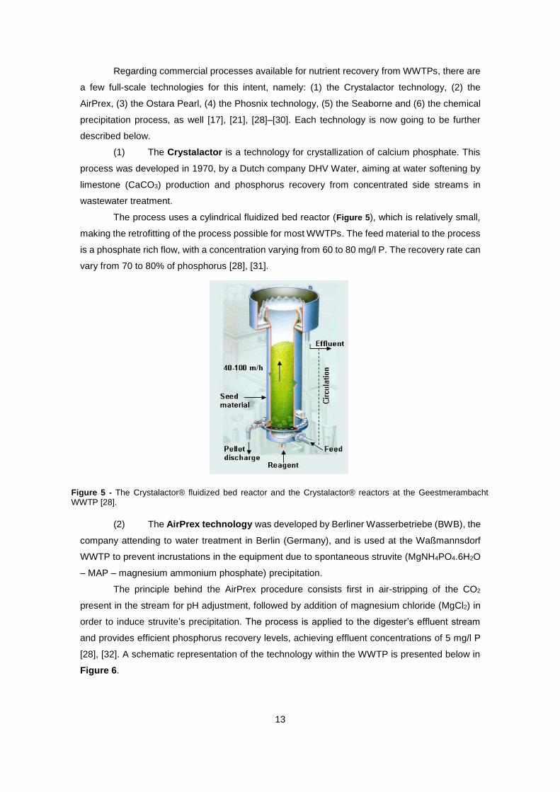
(1) The Crystalactor is a technology for crystallization of calcium phosphate. This
process was developed in 1970, by a Dutch company DHV Water, aiming at water softening by
limestone (CaCO3) production and phosphorus recovery from concentrated side streams in
wastewater treatment.
The process uses a cylindrical fluidized bed reactor (Figure 5), which is relatively small,
making the retrofitting of the process possible for most WWTPs. The feed material to the process
is a phosphate rich flow, with a concentration varying from 60 to 80 mg/l P. The recovery rate can
vary from 70 to 80% of phosphorus [28], [31].
(2) The AirPrex technology was developed by Berliner Wasserbetriebe (BWB), the
company attending to water treatment in Berlin (Germany), and is used at the Waßmannsdorf
WWTP to prevent incrustations in the equipment due to spontaneous struvite (MgNH4PO4.6H2O
– MAP – magnesium ammonium phosphate) precipitation.
The principle behind the AirPrex procedure consists first in air-stripping of the CO2
present in the stream for pH adjustment, followed by addition of magnesium chloride (MgCl2) in
order to induce struvite’s precipitation. The process is applied to the digester’s effluent stream
and provides efficient phosphorus recovery levels, achieving effluent concentrations of 5 mg/l P
[28], [32]. A schematic representation of the technology within the WWTP is presented below in
Figure 6.
Figure 5 - The Crystalactor® fluidized bed reactor and the Crystalactor® reactors at the Geestmerambacht WWTP [28].

14
(3) The Ostara Pearl® is a patented process, developed in University of British
Columbia (Canada).
The process consists of a fluidized bed reactor, which recovers nutrients from sludge
liquor as struvite (MgNH4PO4.6H2O), as shown in Figure 7. The Ostara Group markets the final
product under the name Crystal Green™ and it is used as a slow release fertilizer.
Typically, the process removes 85 % of phosphorus and 10–15% of ammonium present
in the influent stream [28], [33]. A schematic representation of the technology within the WWTP
is presented below in Figure 7.
(4) The Phosnix technology was developed in Japan by Unitika Ltd Environmental
and Engineering Div and it allows for phosphorus recovery in the form of struvite, which is
commercialized as an agricultural fertilizer.
Phosnix reactors have different capacities, being able to treat streams with flow rates
between 150 to 1000 m3/d. The process is feasible for streams with phosphorus concentrations
ranging from 100 to 150 mg/ of P and allows recovery yields between 80 to 90%.
It is a side stream process that can treat water from a number of processes including
digester, industrial, and biological nutrient removal systems. The inflow to the reactor is the liquid-
Figure 7 – Schematic representation of the Ostara Pearl® process. [28]
Figure 6 - The AirPrex procedure [28], [32].

15
phase from the sludge dewatering unit [28], [34]. The process can be described by the following
reaction, presented in equation (1).
𝑀𝑔(𝑂𝐻)2 + 𝑁𝐻4+ + 𝑃𝑂4
3− → 𝑀𝑔𝑁𝐻4𝑃𝑂4. 6𝐻2𝑂 (1)
The effluent from the Phosnix reactor is the transferred to the beginning of the secondary
treatment process, as exemplified below in Figure 8
A full-scale application has been in use in Lake Shinji Eastern Clarification Centre of
Shimane Prefecture (SECC), Japan, since 1998.
(5) The Seaborne process was developed by the Seaborne Environmental Research
Laboratory (EPM AG), in Germany. It is a complex network of unit operations, suitable for
recovering nutrients from various biomasses.
The process consists mainly of three operations, namely, an acid leaching step, followed
by a step for heavy metals removal and finally a struvite precipitation step. The influent to the
process is the effluent stream from the digestion process and typically presents a phosphorus
concentration of 600 mg/l P. The phosphorus recovery of the process is approximately equal to
90% [27], [28].
A schematic representation of the process and its integration within the WWTP is
presented in Figure 9.
Figure 8 – Schematic representation of the Phosnix process in the WWTP.
Figure 9 – Schematic representation of the Seaborne process in the WWTP.

16
(6) The Chemical Precipitation is a non-proprietary process, but it is a fully studied and
comprehended technique, in everything comparable to a full-scale technology. It can be applied
as a nutrient recovery technique for low-nutrient concentration streams, for the recovery of
phosphorus from the effluent stream, for example.
The chemical precipitation process can remove phosphorus through the addition of one
the following reactants:
(a) Metal salts, as described in equation (2).
𝑀𝑒3+(𝑎𝑞) + 𝑃𝑂43−(𝑎𝑞) → 𝑀𝑒𝑃𝑂4(𝑠) (2)
(b) Lime (Ca(OH)2), as described in (3) and (4).
𝐶𝑎(𝑂𝐻)2(𝑎𝑞) + 𝐻2𝑃𝑂4− → 𝐶𝑎𝐻𝑃𝑂4(𝑠) + 𝐻2𝑂 + 𝑂𝐻− (3)
5𝐶𝑎2+(𝑎𝑞) + 3𝑃𝑂43−(𝑎𝑞) + 𝑂𝐻− → 𝐶𝑎3(𝑃𝑂4)3𝑂𝐻(𝑠) (4)
Addition of iron salts, such as iron sulphate (FeSO4), results in the formation of an iron
phosphate precipitate (FePO4), which is an agricultural fertilizer and has commercial value. At the
end of the process, phosphorus concentrations under 1 mg/l P can be achieved.
The aforementioned full-scale technologies for resource recovery from wastewater
treatment plants are summarized below on Table 3.
Table 3 – Summary of the full-scale technologies for resource-recovery.
Resource
Recovered Technology
Start-up
Date
Feed
Material Method Final Product
Onsite Energy Generation
Cambi THP 2009 Non-
digested Sludge
Thermal Hydrolysis
(Batch)
Digested Sludge
Exelys 2011 Non-
digested Sludge
Thermal Hydrolysis
(Continuous)
Digested Sludge
Nutrients Recovery
Crystalactor 1988 Liquid Crystallization Iron Phosphate
AirPrex 2010 Liquid Crystallization Calcium
Phosphate
Ostara Pearl 2007 Digested Sludge
Crystallization Struvite
Phosnix 1998 Liquid Crystallization Struvite
Seaborne 2005 Liquid Acid Leaching/ Crystallization
Struvite
Chemical Precipitation
--- Digested Sludge
Chemical Precipitation Struvite
In order to identify the most efficient way of including resource recovery into a WWTP it
is necessary to test different control strategies. Mathematical modelling is the best methodology
to continuously evaluate the performance of wastewater treatment systems [11]. In this way, the
following sub-chapter presents a literature review on the initial mathematical models used for
wastewater treatment and on the current state of wastewater treatment modelling.

17
2.3 MODELLING OF WASTEWATER TREATMENT SYSTEMS
Modelling is used as a methodology to define complex systems in a more simplified way,
in order to allow for a better understanding of the relevant characteristics of those systems and
to predict its behaviour. Not only modelling allows one to get insight into a plant’s performance,
but it also enables (i) the evaluation of different possible scenarios for further upgrading the plant,
(ii) supporting management decisions,(iii) developing new control schemes and, lastly, (iv)
providing operator training. All of these can be achieved with lower costs and under a shorter
period of time, than using experimental studies to study the system [11].
The activated sludge unit plays a central role in wastewater treatment because it is the
most widely used biological process for treatment of liquid waste; therefore, this treatment unit
was the first one to be modelled. Extensive studies have been conducted on the activated sludge
unit and resulted in the development of several models to describe it. Despite of that, there is a
general acceptance towards the models of the Activated Sludge Models (ASMs) family, namely
the ASM1 [35], the ASM2 [11], the ASM2d [36] and the ASM3 [11], proposed by the International
Water Association (IWA). The main biological processes described in the referred ASMs are
summarized in Table 4. A brief introduction to the Anaerobic Digestion Model No. 1 (ADM1) is
presented as well.
Table 4 – Summary of the existing ASMs for the activated sludge unit. Legend: Den. PAO (Denitrifying PAO
activity included in the model), DR (death regeneration concept), EA (electron acceptor depending), ER
(endogenous respiration concept), Cst (non-electron acceptor depending). The dot symbol, • , identifies that
a given process is present in a model [11].
Mo
del
Nitrificatio
n
Denitrificatio
n
Hete
rotr
ophic
/ A
uto
trophic
Deca
y
Hydro
lysis
EB
PR
Denitrify
ing
PA
O
Lysis
of P
AO
/ P
HA
Fe
rme
nta
tio
n
Chem
ical P
Rem
oval
Num
ber
of
Reactio
ns
Num
ber
of
Sta
te V
aria
ble
s
ASM1 DR, Cst EA 8 13
ASM2 DR, Cst EA Cst 19 19
ASM2d DR, Cst EA Cst 21 19
ASM3 ER, EA Cst 12 13
ASM3-bioP ER, EA Cst EA 23 17
From the models mentioned above, the Activated Sludge Model No. 1 (ASM1) was the first
to be modelled and was also the first to be implemented in practise. In this way, this model is
used as a reference by the research community for modelling the activated sludge unit [11]. The
ASM1 model will be described in detail in the sub-chapter 2.3.1. The other models of the ASM
family are briefly presented in the sub-chapter 2.3.2.
2.3.1 ASM1 - ACTIVATED SLUDGE MODEL NUMBER 1
The ASM1 was primarily developed by Henze et al. (1987), for the removal of organic
compounds and nitrogen, with simultaneous consumption of oxygen and nitrate as electron

18
accepters, from municipal waste activated sludge plants. Also, ASM1 aims at providing a good
description of the sludge production [11].
The model was firstly developed based on 3 base-components, namely dissolved oxygen
(SO), dissolved organic substrate (SS) and heterotrophic biomass (XH), and 2 main conversion
processes: (1) aerobic biomass growth and (2) lysis of biomass. COD was adopted as the
measure of the concentration of organic matter [11].
Monod kinetic equation is used in the ASM1 to describe the aerobic biomass growth, as
shown below in equation (5):
𝐴𝑒𝑟𝑜𝑏𝑖𝑐 𝐺𝑟𝑜𝑤𝑡ℎ 𝑜𝑓 𝐻𝑒𝑡𝑒𝑟𝑜𝑡𝑟𝑜𝑝ℎ𝑠 = ��𝐻 × (𝑆𝑆
𝑆𝑆 + 𝐾𝑆
)(𝑆𝑂
𝐾𝑂,𝐻 + 𝑆𝑂
)𝑋𝐵,𝐻 (5)
where ��𝐻 is the maximum specific growth rate of heterotrophic biomass (𝑑−1), 𝐾𝑆 is the half-
saturation coefficient for heterotrophic biomass (𝑔 𝐶𝑂𝐷 𝑚3⁄ ) , 𝑆𝑆 is the readily biodegradable
substrate (𝑔 𝐶𝑂𝐷 𝑚3⁄ ) , 𝑆𝑂 is the oxygen (𝑔(−𝐶𝑂𝐷) 𝑚3⁄ ) , 𝐾𝑂,𝐻 is the oxygen half-saturation
coefficient for denitrifying heterotrophic biomass (𝑔 𝑂2 𝑚3⁄ ) and 𝑋𝐵,𝐻 is the active heterotrophic
biomass (𝑔 𝐶𝑂𝐷 𝑚3)⁄ . ��𝐻 and Ki are empirical coefficients of the Monod equation [11], [35].
Monod’s model assumes that the growth rate of biomass is related to the concentration of
a single growth limiting substrate, however, biomass growth rate is dependent on multiple
substrates, as in the case of the anoxic growth of heterotrophs, as presented in equation (6).
𝐴𝑛𝑜𝑥𝑖𝑐 𝐺𝑟𝑜𝑤𝑡ℎ 𝑜𝑓 𝐻𝑒𝑡𝑒𝑟𝑜𝑡𝑟𝑜𝑝ℎ𝑠 = ��𝐻 × (𝑆𝑆
𝑆𝑆 + 𝐾𝑆
)(𝐾𝑂,𝐻
𝑆𝑂 + 𝐾𝑂,𝐻
)(𝑆𝑁𝑂
𝑆𝑁𝑂 + 𝐾𝑁𝑂
)𝜂𝑔𝑋𝐵,𝐻 (6)
where 𝑆𝑁𝑂 is the nitrate and nitrite nitrogen (𝑔𝑁𝑂3 − 𝑁/ 𝑚3), 𝐾𝑁𝑂 is the nitrate half-saturation
coefficient for denitrifying heterotrophic biomass (𝑔 𝑁𝑂3 − 𝑁 𝑚3⁄ ) and 𝜂𝑔 is correction factor for
��𝐻 under anoxic conditions (dimensionless) [11], [35].
The lysis process is modelled in the ASM1 model as a 1st order process, where biomass is
lysed in proportion to the active heterotrophic biomass, resulting in equation (7).
𝐵𝑖𝑜𝑚𝑎𝑠𝑠𝐿𝑦𝑠𝑒𝑑 (𝑔 𝐶𝑂𝐷/ 𝑚3) = 𝑏𝐻 . 𝑋𝐵,𝐻 (7)
where 𝑏𝐻 is the decay coefficient for heterotrophic biomass (𝑑−1).
In the ASM1 model, biomass degradation is performed in two processes: a relatively rapid
process of biodegradation of part of the COD (RBCOD), comprising of organics such as volatile
fatty acids (VFAs) and glucose, and a relatively slow process of the COD degradation (SBCOD)
(cellulose, starch, proteins, etc) [35], [11].
It is also assumed that the SBCOD is converted into RBCOD by the relatively slow process
of hydrolysis, introducing a new process to the ASM1. To model this process the following kinetic
equation, equation (8), was considered:
𝐵𝑖𝑜𝑚𝑎𝑠𝑠𝐻𝑦𝑑𝑟𝑜𝑙𝑖𝑠𝑒𝑑 (𝑔 𝐶𝑂𝐷
𝑚3) = 𝑘ℎ.
(𝑋𝑆 𝑋𝐵,𝐻⁄ )
𝐾𝑋 + (𝑋𝑆 𝑋𝐵,𝐻)⁄[
𝑆𝑂
𝐾𝑂,𝐻 + 𝑆𝑂
+ 𝜂ℎ(𝐾𝑂,𝐻
𝐾𝑂,𝐻 + 𝑆𝑂
)(𝑆𝑁𝑂
𝐾𝑁𝑂 + 𝑆𝑁𝑂
)]. 𝑋𝐵,𝐻 (8)
where 𝑘ℎ is the maximum specific hydrolysis rate (𝑔 𝑆𝐵𝐶𝑂𝐷/ (𝑔 𝑐𝑒𝑙𝑙 𝐶𝑂𝐷. 𝑑)) and 𝜂ℎ is the
correction factor for hydrolysis under anoxic conditions (dimensionless) [35], [11].

19
Lastly, the model also considers the existence of an influent non-biodegradable fraction of
COD (being inert, and also particulate organic matter),which accumulates in the reactor: XI [35],
[11].
2.3.1.1 ASM1 MATRIX REPRESENTATION
Complex mathematical models, as the case of the ASM1 model, are recommended to be
described in a matrix representation, allowing for an explicit presentation of the compounds and
processes included in the model and their interactions. This representation also enables for an
easy comparison of different models and facilitates their introduction into a computer program.
The matrix representation consists of a matrix which is represented by a number of columns
and rows. One column for each compound (represented by the generic letter i) and one row for
each process (represented by the generic letter j). The compounds are presented as symbols
listed at the head of the appropriate column including a row with its dimensions. The biological
processes occurring in the system, that affect the compounds considered, are itemized down the
left-hand side of the matrix. The process rates are formulated mathematically and listed in the
right-hand side of the stoichiometry matrix in line with the respective process. Along each process
row, the stoichiometric coefficient for conversion of one compound into another is inserted so that
each compound column lists the stoichiometric coefficients for the processes that influence that
compound. If the stoichiometric coefficient is equal to zero, then it is generally not printed in the
matrix. The sign convention used in the matrix for each compound per se is ’negative for
consumption’ and ‘positive for production’, as in the case of process rates [11].
An example of the described format can be observed in Table 5.
Table 5 - Example of a simple stoichiometric matrix for activated sludge modelling (adapted from [11]).
Components i 1: SO 2: SS 3: XH Process Rate Equation, ρj
List of Processes j
Aerobic Growth −1
𝑌𝐻
+ 1 −1
𝑌𝐻
+1 𝜇𝐻𝑚𝑎𝑥 .
𝑆𝑆
𝐾𝑆 + 𝑆𝑆
. 𝑋𝐻
Lysis +1 -1 𝑏𝐻 . 𝑋𝐻
Observed Transformation Rate ri
𝑟𝑖 = ∑ 𝑣𝑖,𝑗 . 𝜌𝑗 [𝑀𝑖𝐿−3𝑇−1]
Definition of Stoichiometric Parameters:
YH: Heterotrophic Yield Coefficient [MH MS
-1] Dis
solv
ed
Oxygen (
O2)
Dis
solv
ed
Org
anic
Substr
ate
(C
OD
)
Hete
rotr
oph
ic
Bio
mass (
CO
D)
Definition of kinetic parameters: µH
max - Maximum specific growth rate [T-1] KS - Saturation coefficient for substrate
[MCODL-3] bH - Rate constant for decay [T-1]
2.3.2 OTHER ACTIVATED SLUDGE MODELS – ASM2, ASM2D, ASM3
Continuous development of models for characterization of the activated sludge unit allows
for a more broad choice when selecting the model to work with. Each ASM model is focussed on
a specific topic allowing the developer to use the variation that is more appropriate for his case

20
study. This type of model development also prevents the continue increase of the model size [11].
A brief description of the ASM family models ASM3, ASM2 and ASM2d is presented ahead.
The activated Sludge Model No. 2 (ASM2), developed in 1995, was created aiming at
including an Enhanced Biological Phosphorus Removal (EBPR) module. Chemical precipitation
of phosphorus (CPR) was also included in the ASM2 model. The model description states
explicitly that it includes EBPR processes, but does not include all observed phenomena yet. In
this sense, the Activated Sludge Model No. 2d (ASM2d) was created in 1999, to fill in that gap. In
this model, the denitrifying activity of phosphate accumulating organisms (PAOs) was considered,
allowing for a better description of the dynamics for phosphate and nitrate conversion rates. [11],
[36].
The activated Sludge Model No. 3 (ASM3) was developed in 1999, as a correction to
ASM1, being in everything similar to the latter. The main difference in the ASM3 model is the
recognition of the importance of three rates of oxygen consumption in the process: the rapid rate
of oxygen consumption for degradation of RBCOD, slow rate associated with degradation of
SBCOD, and an even sower endogenous oxygen uptake rate (OUR). As so, the ASM3 model
performs better than the ASM1 model in situations where the storage of readily biodegradable
substrate is significant (industrial wastewater) or for plants with substantial non-aerated zones
[11].
Even though several models have been developed for improving the performance of the
activated sludge unit process, it is difficult to compare or evaluate them due to the presence of
too many confounding influences that have an impact on wastewater treatment systems. This
constraint created the need for a standardised tool that would allow to objectively compare
different control strategies applied to wastewater treatment systems, which led to the
development of a standardised simulation protocol – a ‘simulation benchmark’ [37]. A description
of the concept and a literature review of the benchmark simulation models is presented next.
2.3.3 BENCHMARK SIMULATION MODELS
Benchmark Simulation Models (BSM) are a standardised simulation protocol which is
used as performance assessment and evaluation of control strategies for wastewater treatment
systems. The benchmark is a simulation environment which defines a plant layout, a simulation
model, influent loads, test procedures and evaluation criteria; once the user validates the
simulation code, any control strategy can be applied and the performance can be evaluated
according to a defined set of criteria [8], [37]–[41].
From 1998 to 2004, the development of benchmark models has been undertaken in
Europe by Working Groups of COST Action 682 and 624; this work is now continued under the
umbrella of an International Wastewater Association Task (IWA) Group [38].
The first benchmark simulation model to be developed was the Benchmark Simulation
Model No. 1 (BSM1), in 2002, which primary purpose has been to create a platform for control
strategy benchmarking of activated sludge processed. However, as previously mentioned, the
current state of mind regarding wastewater treatment is set towards a “plant-wide approach”, with

21
the inclusion of both water and sludge lines in wastewater treatment systems. In this way,
modelling of wastewater treatment systems can no longer be a simple compilation of solutions
achieved for the design or operation of each individual unit-process, as in the case of the ASM
models [42]. Like so, the existing benchmark simulation models could no longer satisfy the
necessary requirements, introducing the need for the creation of an additional benchmark model,
the Benchmark Simulation Model No. 2 (BSM2), in 2007. The BSM1 and BSM2 are further
detailed below.
2.3.3.1 BSM1 – BENCHMARK SIMULATION MODEL NO. 1
The BSM1, was developed by Copp, in 2002, and its main goal is to allow for objective
and unbiased comparison of carbon and nitrogen removal activated sludge control strategies [37],
[43]. In this way, the BSM1 is composed of a five-compartment activated sludge reactor consisting
of two anoxic tanks, followed by three aerobic tanks. It thus combines nitrification with pre-
denitrification in a configuration that is commonly used for achieving biological nitrogen removal
in full-scale plants. The activated sludge reactors are followed by a secondary clarifier, as
schematically represented in Figure 10.
The success of the BSM1 as efficient platform for control strategies comparison in
biological nitrogen removal activated sludge plants is proven by the large number of scientific
papers using it. However, even though the BSM1 is recognized as a very flexible tool, it is not
intended for long-term evaluations, which are vital in order to perform a fully understanding of the
optimum solution for wastewater treatment systems. In this way, there was the need to create the
BSM1-Long Term (BSM1-LT) model in 2004. The BSM1-LT model extends the evaluation period
files to 52 weeks (1 year) and includes long-term dynamics, such as influent with dry and rain
weather events tested over extended periods [38], [40].
Figure 10 – General overview of the BSM1 plant [37].

22
2.3.3.2 BSM2 – BENCHMARK SIMULATION MODEL NO. 2
The BSM2, by Jeppsson et al. (2007), is an upgrade from the BSM1-LT. The main
alterations include the addition of a pre-treatment step, with the introduction of a primary clarifier
unit, and the addition of a sludge train, which comprises a thickener, for the sludge wasted from
the BSM1 secondary clarifier, an anaerobic digester, for treatment of thickened secondary sludge
and solids wasted from the primary clarifier, and a dewatering unit, for the dewatering of the
digested sludge [8], [38], [40], as schematically represented in Figure 11.
The BSM2 is the benchmark simulation model currently used for testing control strategies
applied to wastewater treatment systems. As so, the BSM2 is used in the present work as a
starting setting a wastewater treatment plant. In this sense, the selection of the full-scale
technologies to retrofit wastewater treatment plants with resource recovery was based on the
BSM2 layout.
With the aim of broadening the spectrum of resources recovered from the BSM2 plant,
the Exelys technology was chosen for onsite energy generation. From the nutrient recovery full-
scale technologies presented, the chemical precipitation process and Phosnix technology were
selected, enabling resource recovery from two different streams.
Even though the Crystalactor technology was a good alternative to the chemical
precipitation process, for resource recovery from the effluent stream of the activated sludge unit,
the Crystalactor technology was not fit for the BSM2 configuration, because this process is
intended for streams with high phosphorus concentrations, only achieved in secondary treatments
that include biological phosphorus removal processes, such as the EBPR systems, which is not
the case of the BSM2. Regarding the remaining full-scale technologies presented for resource
Figure 11 – General overview of the BSM2 plant [8].

23
recovery, whether due to increased operating costs, less knowledge or higher complexity, this
technologies were not preferred over the Phosnix technology.
2.3.4 ADM1 – ANAEROBIC DIGESTION MODEL NO. 1
The ADM1 was created by Batstone et al. (2002), to overcome limitations of previously
developed models for the anaerobic digestion process, due to over-specificity and inability to be
more widely applied. Therefore, the ADM1 model can be regarded as a widely-applicable,
baseline, or uniform platform that further welcomes any necessary application-specific
refinements or modifications of certain processes.
In a general description, the ADM1 model simulates major processes of the anaerobic
digestion process, which are associated with degrading complex organic substrates into proteins,
fats, carbohydrates and inert compounds. These degradation products are then hydrolysed to
amino acids, long chain fatty acids (LCFA), and sugars, respectively. Methane gas is produced
by both aceticlastic methanogenic cleavage of acetate and hydrogenotrophic methanogenic
reduction of CO2 by H2. Extra-cellular enzymes are assumed to catalyse biochemical reactions
involving biologically-available organic substrates and all extra-cellular ADM1 biochemical
reactions are assumed to follow empirically-based 1st order rete law kinetics, and all intra-cellular
ADM1 biochemical reactions are assumed to follow Monod-type substrate uptake kinetics.
Substrate uptake reaction rates are proportional to the biomass growth rate and biomass
concentration.
The ADM1 model has been widely applied and validated in simulating the anaerobic
digestion of several organic wastes [44], [45].
2.4 CHAPTER CONCLUSIONS
The continuous development of wastewater treatment systems aims at improving the
performance of these plants in the most efficient way possible. Over the past decades, there has
been a growing awareness towards the resource depletion problem, and wastewater treatment
plants are an example of the large resources consumers. In this sense, resource recovery is used
as a way of mitigating the large consumption of resource in wastewater treatment plants.
There are two main ways of implementing resource recovery in WWTPs, namely, through
onsite energy generation and nutrient recovery. The three full-scale technologies for resource
recovery tested in this dissertation were the chemical precipitation process, the Exelys technology
and the Phosnix technology.
Mathematical modelling of complex systems, such as wastewater treatment systems, is
the most efficient methodology for studying the best way of maximizing resource recovery in
WWTP. In this dissertation, the Benchmark Simulation Model No.2 (BSM2) was used as a starting
wastewater treatment plant scenario. The BSM2 was retrofitted in order to include the three
resource recovery, which best fitted to the BSM2 layout.

24
3 MODEL DEVELOPMENT
Aiming at developing a simulation model for wastewater treatment plants which includes
onsite recovery of added-value products, an already existing simulation model for full-scale
wastewater treatment systems, the Benchmark Simulation Model No. 2 (BSM2) by Jeppsson et
al. (2007), was extended. MATLAB/Simulink software was used to extend the model.
All the modifications applied to the main model are going to be described in this chapter.
More specifically, the present chapter is divided into four Sections. Section 3.1 presents an
overview of the model’s influent file, operating conditions, components and their main
characteristics (the ASM1 model and ADM1 model are described in further detail). Section 3.2
describes the different full-scale simulation scenarios considered for the present work. Section
3.3 outlines the assumptions made and the equations used in order to introduce the recovery of
added-value products within the reference BSM2. Section 3.4 summarizes the equations used for
performing an economic evaluation on the results obtained from the various simulation scenarios
considered. Finally, Section 3.5 has the conclusions of the chapter.
3.1 BENCHMARK SIMULATION MODEL NO. 2 OVERVIEW
The constant influent used in the BSM2 is provided in the following table, Table 6.
Table 6 – Influent values considered in the BSM2.
Variable Value Unit
SI,stab 27.22619062 g COD /m3
SS,stab 58.17618568 g COD /m3
XI,stab 92.49900106 g COD /m3
XS,stab 363.943473 g COD /m3
XB,H,stab 363.943473 g COD /m3
XB,A,stab 50.68328815 g COD /m3
XP,stab 0 g COD /m3
SO,stab 0 g (-COD) /m3
SNO,stab 0 g N /m3
SNH,stab 0 g N /m3
SND,stab 23.85946563 g N /m3
XND,stab 5.651606031 g N /m3
SALK,stab 16.12981606 mole /m3
TSSstab 7 g /m3
Qi,stab 380.3443217 m3/d
Tstab 20648.36121 ºC

25
The operational conditions assumed in the BSM2 are presented in Table 7.
Table 7 – Operational conditions assumed in the BSM2.
Operational Condition Value Units
Internal recycle flow rate (Qint) 61944 m3/d
External recycle flow rate (Qr) 20648 m3/d
Wastage flow rate (Qw) 300 m3/d
External carbon flow rate in the 1st anoxic tank (QEC1) 2 m3/d
External carbon concentration 400000 g COD/m3
Oxygen transfer coefficients KLa3= KLa4=120
KLa5=60 d-1
Flow rate from the reject water storage tank (Qst,set) 0 m3/d
The main components of the plant model (see also Figure 11) are summarized below in
Table 8.
Table 8 – Summary of the main components in the BSM2 [38].
Component Model Characteristics
Primary clarifier Otterpohl and Freund (1992) [46] - 50% solids removal efficiency - no biological activity
Five-reactor nitrogen removal activated sludge system
ASM1 (Henze et al., 1987) [35] ---
Secondary clarifier Takács et al. (1991) [47] - no biological activity
Gravity thickener Ideal and continuous process - 98% solids removal efficiency - no biological activity
Anaerobic digester ADM1 (Batstone et al., 2002) [45] ---
Dewatering unit Ideal and continuous process - 98% solids removal efficiency - no biological activity
AD/ AS model interfaces Nopens et al. (2007) [48] ---
Storage tank Continuous process - controllable output pumping capacity - no biological activity
Influent wastewater Gernaey et al. (2005:2006) [38] - 609-day influent data file (data every 15 minutes)
Further information about BSM2 can be find in Jeppsson et al. (2007) and Gernaey et al.
(2004). The ASM1 and ADM1 describe complex biological processes for the activated sludge
units and the anaerobic digester, respectively, being key-models for the BSM2. In this way, the
ASM1 and ADM1 are further detailed below.
3.1.1 ASM1-ACTIVATED SLUDGE UNIT
A schematic representation of the BSM1 has been previously presented in Figure 10.
Each of the first two anoxic tanks have a volume of 1500 m3 and use a default kLa
coefficient of 2 d-1 to model the mixing regime. Each of the three subsequent aerobic tanks have
a volume of 3000 m3 and fixed kLa values of 120 d-1 for the first two and 60 d-1 for the last. Two
recycles are included: (a) an external recycle, where settled biomass is carried from the

26
secondary clarifier underflow to the 1st anoxic tank; and (b) an internal recycle which carries
nitrogen oxides from the 5th to the 1st biological tank. Supplementary carbon is dosed to the first
anoxic tank, at a default flow rate of 2 m3/d and concentration of 400 kg COD/m3. The default
wastage sludge flow rate is equal to 300 m3/d and is fed from the secondary settler into the
thickener. The secondary clarifier presents a fixed volume of 6000 m3 (area of 1500 m2, depth of
4 m).
The ASM1 state variables, associated symbols and the state variable units are presented
next in Table 9.
Table 9 - State variables for the IAWQ Activated Sludge Model No. 1 (ASM1) [35].
Component State Variable Description State Symbol Units
1 Soluble Inert Organic Matter SI g COD /m3
2 Readily biodegradable substrate SS g COD /m3
3 Particulate inert organic matter XI g COD /m3
4 Slowly biodegradable substrate XS g COD /m3
5 Active heterotrophic biomass XB,H g COD /m3
6 Active autotrophic biomass XB,A g COD /m3
7 Particulate products arising from biomass
decay XP g COD /m3
8 Oxygen SO g(-COD) /m3
9 Nitrate and nitrite nitrogen SNO g N /m3
10 NH4+ + NH3 nitrogen SNH g N /m3
11 Soluble biodegradable organic nitrogen SND g N /m3
12 Particulate biodegradable organic nitrogen XND g N /m3
13 Alkalinity SALK mol/ L
The rate equations chosen to represent the fundamental processes of the activated
sludge-unit are listed down in Table 10.
Table 10 - Rate equations for all processes included in ASM1 [35].
Process Process Process Rate Equation: 𝝆𝒋,, kg COD/(m3.d)
1 Aerobic Growth of
Heterotrophs ��𝐻(
𝑆𝑆
𝐾𝑆 + 𝑆𝑆
)(𝑆𝑂
𝐾𝑂,𝐻 + 𝑆𝑂
)𝑋𝐵,𝐻
2 Anoxic Growth of
Heterotrophs ��𝐻(
𝑆𝑆
𝐾𝑆 + 𝑆𝑆
)(𝐾𝑂,𝐻
𝐾𝑂,𝐻 + 𝑆𝑂
)(𝑆𝑁𝑂
𝐾𝑁𝑂 + 𝑆𝑁𝑂
)𝜂𝑔𝑋𝐵,𝐻
3 Aerobic Growth of
Autotrophs ��𝐴(
𝑆𝑁𝐻
𝐾𝑁𝐻 + 𝑆𝑁𝐻
)(𝑆𝑂
𝐾𝑂,𝐴 + 𝑆𝑂
)𝑋𝐵,𝐴
4 “Decay” of Heterotrophs 𝑏𝐻𝑋𝐵,𝐻
5 “Decay” of Autotrophs 𝑏𝐴𝑋𝐵,𝐴
6 Ammonification of Soluble
Organic Nitrogen 𝑘𝑎𝑆𝑁𝑂𝑋𝐵,𝐻
7 “Hydrolysis” of Particulate
Organics 𝑘ℎ
𝑋𝑆 𝑋𝐵,𝐻⁄
𝐾𝑋 + (𝑋𝑆 𝑋𝐵,𝐻⁄ )[(
𝑆𝑂
𝐾𝑂,𝐻 + 𝑆𝑂
) + (𝐾𝑂,𝐻
𝐾𝑂,𝐻 + 𝑆𝑂
)(𝑆𝑁𝑂
𝐾𝑁𝑂 + 𝑆𝑁𝑂
)] 𝑋𝐵,𝐻
8 “Hydrolysis” of Particulate
Organic Nitrogen 𝜌7(𝑋𝑁𝐷/𝑋𝑆)

27
A matrix representation of ASM1, previously explained in Section 2.3.1.1, is presented in
Table 11. This model representation is included as a reference only, a complete description of
the model and its development are available elsewhere [35].
The stoichiometric and kinetic parameters values are listed in attachment in Table 37
and Table 38, respectively, in the Section 8.1.1.

28
Table 11 - Matrix representation of ASM1 showing the processes, components, process rate equations, and stoichiometry [35].
Component i → 1 2 3 4 5 6 7 8 9 10 11 12 13 Process
Rate Process j ↓ 𝑺𝑰 𝑺𝑺 𝑿𝑰 𝑿𝑺 𝑿𝑩.𝑯 𝑿𝑩.𝑨 𝑿𝑷 𝑺𝑶 𝑺𝑵𝑶 𝑺𝑵𝑯 𝑺𝑵𝑫 𝑿𝑵𝑫 𝑺𝑨𝑳𝑲
1 Aerobic Growth of Heterotrophs −1
𝑌𝐻
1 −1 − 𝑌𝐻
𝑌𝐻
−𝑖𝑋𝐵 −𝑖𝑋𝐵
14 1
2 Anoxic Growth of Heterotrophs −1
𝑌𝐻
1 −1 − 𝑌𝐻
2.86𝑌𝐻
−𝑖𝑋𝐵 1 − 𝑌𝐻
14 × 2.86𝑌𝐻
−𝑖𝑋𝐵
14 2
3 Aerobic Growth of Autotrophs 1 1 − 𝑌𝐻
𝑌𝐻
1
𝑌𝐴
−𝑖𝑋𝐵 −1
𝑌𝐴
−𝑖𝑋𝐵
14−
1
7𝑌𝐴
3
4 “Decay” of Heterotrophs 1 − 𝑓𝑝 -1 𝑓𝑝 𝑖𝑋𝐵 − 𝑓𝑝𝑖𝑋𝑃 4
5 “Decay” of Autotrophs 1 − 𝑓𝑝 -1 𝑓𝑝 𝑖𝑋𝐵 − 𝑓𝑝𝑖𝑋𝑃 5
6 Ammonification of Soluble Organic
Nitrogen 1 -1
1
14 6
7 “Hydrolysis” of Entrapped Organics 1 -1 7
8 “Hydrolysis” of Entrapped Organic
Nitrogen 1 -1 8
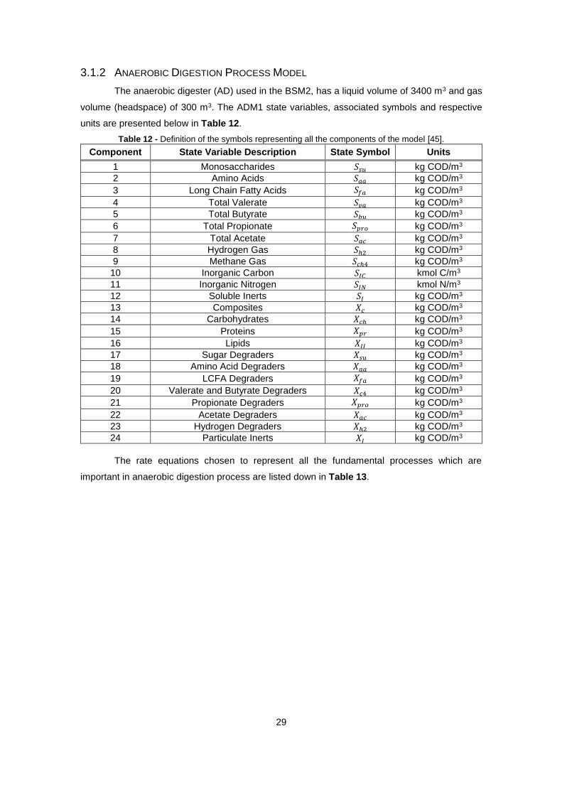
29
3.1.2 ANAEROBIC DIGESTION PROCESS MODEL
The anaerobic digester (AD) used in the BSM2, has a liquid volume of 3400 m3 and gas
volume (headspace) of 300 m3. The ADM1 state variables, associated symbols and respective
units are presented below in Table 12.
Table 12 - Definition of the symbols representing all the components of the model [45].
Component State Variable Description State Symbol Units
1 Monosaccharides 𝑆𝑠𝑢 kg COD/m3
2 Amino Acids 𝑆𝑎𝑎 kg COD/m3
3 Long Chain Fatty Acids 𝑆𝑓𝑎 kg COD/m3
4 Total Valerate 𝑆𝑣𝑎 kg COD/m3
5 Total Butyrate 𝑆𝑏𝑢 kg COD/m3
6 Total Propionate 𝑆𝑝𝑟𝑜 kg COD/m3
7 Total Acetate 𝑆𝑎𝑐 kg COD/m3
8 Hydrogen Gas 𝑆ℎ2 kg COD/m3
9 Methane Gas 𝑆𝑐ℎ4 kg COD/m3
10 Inorganic Carbon 𝑆𝐼𝐶 kmol C/m3
11 Inorganic Nitrogen 𝑆𝐼𝑁 kmol N/m3
12 Soluble Inerts 𝑆𝐼 kg COD/m3
13 Composites 𝑋𝑐 kg COD/m3
14 Carbohydrates 𝑋𝑐ℎ kg COD/m3
15 Proteins 𝑋𝑝𝑟 kg COD/m3
16 Lipids 𝑋𝐼𝐼 kg COD/m3
17 Sugar Degraders 𝑋𝑠𝑢 kg COD/m3
18 Amino Acid Degraders 𝑋𝑎𝑎 kg COD/m3
19 LCFA Degraders 𝑋𝑓𝑎 kg COD/m3
20 Valerate and Butyrate Degraders 𝑋𝑐4 kg COD/m3
21 Propionate Degraders 𝑋𝑝𝑟𝑜 kg COD/m3
22 Acetate Degraders 𝑋𝑎𝑐 kg COD/m3
23 Hydrogen Degraders 𝑋ℎ2 kg COD/m3
24 Particulate Inerts 𝑋𝐼 kg COD/m3
The rate equations chosen to represent all the fundamental processes which are
important in anaerobic digestion process are listed down in Table 13.
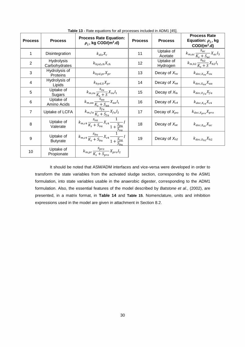
30
Table 13 - Rate equations for all processes included in ADM1 [45].
Process Process Process Rate Equation:
𝝆𝒋,, kg COD/(m3.d) Process Process
Process Rate
Equation: 𝝆𝒋,, kg
COD/(m3.d)
1 Disintegration 𝑘𝑑𝑖𝑠𝑋𝑐 11 Uptake of Acetate
𝑘𝑚,𝑎𝑐
𝑠𝑎𝑐
𝐾𝑠 + 𝑆𝑎𝑐
𝑋𝑎𝑐𝐼3
2 Hydrolysis
Carbohydrates 𝑘ℎ𝑦𝑑,𝑐ℎ𝑋𝑐ℎ 12
Uptake of Hydrogen
𝑘𝑚,ℎ2
𝑠ℎ2
𝐾𝑠 + 𝑆𝑋ℎ2𝐼1
3 Hydrolysis of
Proteins 𝑘ℎ𝑦𝑑,𝑝𝑟𝑋𝑝𝑟 13 Decay of Xsu 𝑘𝑑𝑒𝑐,𝑋𝑠𝑢
𝑋𝑠𝑢
4 Hydrolysis of
Lipids 𝑘ℎ𝑦𝑑,𝑙𝑖𝑋𝑝𝑟 14 Decay of Xaa 𝑘𝑑𝑒𝑐,𝑋𝑎𝑎
𝑋𝑎𝑎
5 Uptake of Sugars
𝑘𝑚,𝑠𝑢
𝑠𝑠𝑢
𝐾𝑠 + 𝑆𝑋𝑠𝑢𝐼1 15 Decay of Xfa 𝑘𝑑𝑒𝑐,𝑋𝑓𝑎
𝑋𝑓𝑎
6 Uptake of
Amino Acids 𝑘𝑚,𝑎𝑎
𝑠𝑎𝑎
𝐾𝑠 + 𝑆𝑎𝑎
𝑋𝑎𝑎𝐼1 16 Decay of Xc4 𝑘𝑑𝑒𝑐,𝑋𝑐4𝑋𝑐4
7 Uptake of LCFA 𝑘𝑚,𝑓𝑎
𝑠𝑓𝑎
𝐾𝑠 + 𝑆𝑓𝑎
𝑋𝑓𝑎𝐼2 17 Decay of Xpro 𝑘𝑑𝑒𝑐,𝑋𝑝𝑟𝑜𝑋𝑝𝑟𝑜
8 Uptake of Valerate
𝑘𝑚,𝑐4
𝑠𝑣𝑎
𝐾𝑠 + 𝑆𝑣𝑎
𝑋𝑐4
1
1 +𝑆𝑏𝑢
𝑆𝑣𝑎
𝐼 18 Decay of Xac 𝑘𝑑𝑒𝑐,𝑋𝑎𝑐
𝑋𝑎𝑐
9 Uptake of Butyrate
𝑘𝑚,𝑐4
𝑠𝑏𝑢
𝐾𝑠 + 𝑆𝑏𝑢
𝑋𝑐4
1
1 +𝑆𝑣𝑎
𝑆𝑏𝑢
𝐼 19 Decay of Xh2 𝑘𝑑𝑒𝑐,𝑋ℎ2
𝑋ℎ2
10 Uptake of Propionate
𝑘𝑚,𝑝𝑟
𝑠𝑝𝑟𝑜
𝐾𝑠 + 𝑆𝑝𝑟𝑜
𝑋𝑝𝑟𝑜𝐼2
It should be noted that ASM/ADM interfaces and vice-versa were developed in order to
transform the state variables from the activated sludge section, corresponding to the ASM1
formulation, into state variables usable in the anaerobic digester, corresponding to the ADM1
formulation. Also, the essential features of the model described by Batstone et al., (2002), are
presented, in a matrix format, in Table 14 and Table 15. Nomenclature, units and inhibition
expressions used in the model are given in attachment in Section 8.2.

31
Table 14 - Biochemical rate coefficients (vi,j) and kinetic rate equations (ρj) for soluble components (i=1-12, j=1-19) in the ADM1 model. Missing values are equal to 0. [45]. Component → 1 2 3 4 5 6 7 8 9 10 11 12
Rate (𝝆𝒋,, kg
COD/(m3.d)) j Process ↓ 𝑺𝒔𝒖 𝑺𝒂𝒂 𝑺𝒇𝒂 𝑺𝒗𝒂 𝑺𝒃𝒖 𝑺𝒑𝒓𝒐 𝑺𝒂𝒄 𝑺𝒉𝟐 𝑺𝒄𝒉𝟒 𝑺𝑰𝑪 𝑺𝑰𝑵 𝑺𝑰
1 Disintegration 𝑓𝑠𝐼,𝑥𝑐 1
2 Hydrolysis
Carbohydrates 1 2
3 Hydrolysis of
Proteins 1 3
4 Hydrolysis of
Lipids
1− 𝑓𝑓𝑎,𝑙𝑖
1− 𝑓𝑓𝑎,𝑙𝑖
4
5 Uptake of
Sugars -1
(1− 𝑌𝑠𝑢)𝑓𝑏𝑢,𝑠𝑢
(1− 𝑌𝑠𝑢)𝑓𝑝𝑟𝑜,𝑠𝑢
(1− 𝑌𝑠𝑢)𝑓𝑎𝑐,𝑠𝑢
(1− 𝑌𝑠𝑢)𝑓ℎ2,𝑠𝑢
− ∑ 𝐶𝑖𝑣𝑖,5
𝑖=9,11−24
−(𝑌𝑠𝑢)𝑁𝑏𝑎𝑐 5
6 Uptake of Amino
Acids -1
(1− 𝑌𝑎𝑎)𝑓𝑣𝑎,𝑎𝑎
(1− 𝑌𝑎𝑎)𝑓𝑏𝑢,𝑎𝑎
(1− 𝑌𝑎𝑎)𝑓𝑝𝑟𝑜,𝑎𝑎
(1− 𝑌𝑎𝑎)𝑓𝑎𝑐,𝑎𝑎
(1− 𝑌𝑎𝑎)𝑓ℎ2,𝑎𝑎
− ∑ 𝐶𝑖𝑣𝑖,6
𝑖=1−9,11−24
𝑁𝑎𝑎
− (𝑌𝑎𝑎)𝑁𝑏𝑎𝑐 6
7 Uptake of LCFA -1 (1 − 𝑌𝑓𝑎)0.7 (1 − 𝑌𝑓𝑎)0.3 −(𝑌𝑓𝑎)𝑁𝑏𝑎𝑐 7
8 Uptake of Valerate
-1 (1 − 𝑌𝑐4)0.54 (1 − 𝑌𝑐4)0.31 (1 − 𝑌𝑐4)0.15 −(𝑌𝑐4)𝑁𝑏𝑎𝑐 8
9 Uptake of Butyrate
-1 (1 − 𝑌𝑐4)0.8 (1 − 𝑌𝑐4)0.2 −(𝑌𝑝𝑟𝑜)𝑁𝑏𝑎𝑐 9
10 Uptake of
Propionate -1
(1
− 𝑌𝑝𝑟𝑜)0.57
(1
− 𝑌𝑝𝑟𝑜)0.43 − ∑ 𝐶𝑖𝑣𝑖,10
𝑖=1−9,11−24
−(𝑌𝑎𝑐)𝑁𝑏𝑎𝑐 10
11 Uptake of Acetate
-1 (1− 𝑌𝑎𝑐)
− ∑ 𝐶𝑖𝑣𝑖,11
𝑖=1−9,11−24
−(𝑌ℎ2)𝑁𝑏𝑎𝑐 11
12 Uptake of Hydrogen
-1 (1− 𝑌ℎ2)
− ∑ 𝐶𝑖𝑣𝑖,12
𝑖=1−9,11−24
12
13 Decay of Xsu 13
14 Decay of Xaa 14
15 Decay of Xfa 15
16 Decay of Xc4 16
17 Decay of Xpro 17
18 Decay of Xac 18
19 Decay of Xh2 19

32
Table 15 - (Continuation of Table 14) Biochemical rate coefficients (vi,j) and kinetic rate equations (ρj) for soluble components (i=1-12, j=1-19) in the ADM1 model. Missing values
are equal to 0 [45]. Component → 13 14 15 16 17 18 19 20 21 22 23 24
Rate (𝝆𝒋,, kg COD/(m3.d)) j Process ↓ 𝑿𝒄 𝑿𝒄𝒉 𝑿𝒑𝒓 𝑿𝑰𝑰 𝑿𝒔𝒖 𝑿𝒂𝒂 𝑿𝒇𝒂 𝑿𝒄𝟒 𝑿𝒑𝒓𝒐 𝑿𝒂𝒄 𝑿𝒉𝟐 𝑿𝑰
1 Disintegration -1 𝑓𝑐ℎ,𝑥𝑐 𝑓𝑝𝑟,𝑥𝑐 𝑓𝑙𝑖,𝑥𝑐 1
2 Hydrolysis Carbohydrates -1 2
3 Hydrolysis of Proteins -1 3
4 Hydrolysis of Lipids -1 4
5 Uptake of Sugars 𝑌𝑠𝑢 5
6 Uptake of Amino Acids 𝑌𝑎𝑎 6
7 Uptake of LCFA 𝑌𝑓𝑎 7
8 Uptake of Valerate 𝑌𝑐4 8
9 Uptake of Butyrate 𝑌𝑐4 9
10 Uptake of Propionate 𝑌𝑝𝑟𝑜 10
11 Uptake of Acetate 𝑌𝑎𝑐 11
12 Uptake of Hydrogen 𝑌ℎ2 12
13 Decay of Xsu 1 -1 13
14 Decay of Xaa 1 -1 14
15 Decay of Xfa 1 -1 15
16 Decay of Xc4 1 -1 16
17 Decay of Xpro 1 -1 17
18 Decay of Xac 1 -1 18
19 Decay of Xh2 1 -1 19

33
3.2 APPLICATION OF DIFFERENT SIMULATION SCENARIOS
The introduction of the three treatment technologies selected for the recovery of added-value
products from the BSM2 plant results in an extended plant-layout, which is schematized in Figure 12.
In order to assess the impact of the introduction of each technology into the BSM2 plant, seven
different treatment combinations were considered. The different combinations are summarized in Table
16.
Table 16 – Simulation scenarios considered.
Scenario Treatment Combinations
C0 BSM2
C1 C0 + Chemical Precipitation (CP)
C2 C0 + Exelys Technology (ET)
C3 C0 + Phosnix Technology (PT)
C4 C0 + CP + ET
C5 C0 + CP + PT
C6 C0 + CP + ET + PT
C7 C0 + ET + PT
Regarding to scenario 1 (C1), it considers only the introduction of the chemical precipitation (CP)
treatment unit into BSM2; scenario 2 (C2) considers only the introduction of the Exelys technology and
scenario 3 (C3) considers only the introduction of the Phosnix technology.
On the other hand, scenario 4 (C4) considers the introduction of the chemical precipitation plus
the Exelys technology; scenario 5 (C5) considers the introduction of the chemical precipitation plus the
Phosnix technology and combination 7 (C7) considers the introduction of the Exelys and Phosnix
technologies. Lastly, scenario 6 (C6) considers the introduction of the chemical precipitation plus the
Exelys and Phosnix technologies into the BSM2 plant.
A superstructure is presented in Figure 13, in order to get a better understanding of how the
different simulation scenarios were generated and included into the reference BSM2. The path enlighten
in grey represents the BSM2 base-case (scenario 0 – C0).
Figure 12 - Schematic representation of the extended BSM2 layout including the three technologies introduced into the BSM2. Each
technology is enlighten with a different colour: the chemical precipitation is represented in red, the thermal hydrolysis – Exelys technology - is represented in green and the struvite precipitation unit – Phosnix technology - is represented in blue. The technologies are generally represented.
FeSO4.7H2O
Mg(OH)2

34
underflow underflow
supernatant
supernatant
Recycled
underflow
Waste
underflow
WW
CP
By-pass
Sewer
System
Primary
Clarifier
Secondary
Treatment
Reject Water
Treatment
Sludge
Thickening
Sludge
Stabilization
Sludge
Dewatering
PC AS
T AD DU
WATER
SLUDGE
Thermal
Hydrolysis
Exelys
Sinks Chemical
Precipitation
By-pass
Phosnix
By-pass 3
STRUVITE
BIOGAS
CO2
FePO4
supernatant
Figure 13 – Superstructure representation of the resource recovery technologies implemented into BSM2 (WW – wastewater, PC – primary clarifier, AS – activated sludge, CP – chemical
precipitation, T - thickener; AD – anaerobic digestion, DU - dewatering unit). The path enlighten in grey represents the BSM2 base-case (scenario 0 – C0). The dewatering unit number 1 is included in the Exelys technology.

35
3.3 MATHEMATICAL FORMULATION AND MODEL ASSUMPTIONS
Once known the key inputs and outputs of the model, it is necessary to define some parameters
that support it. The reference BSM2 has a fully defined influent file, however, it does not include
phosphorus as a state variable. In this way, to be able to recover phosphorus-based fertilizers from the
waste streams of BSM2 plant, the first extension of the model was to introduce soluble phosphorus
(SPO4-P) as an additional input, with an influent concentration of 6,5 g/m3, according to Bozkurt et al.
(2016).
Secondly, it was necessary to account for the necessary alterations in the BSM2 reference model.
Specifically, there was the need to model the release of phosphorus during the anaerobic digestion, as
presented in equation (9):
[𝑆𝑃𝑂4−𝑃]𝑅𝑒𝑙𝑒𝑎𝑠𝑒𝑑 𝐴𝐷 = 𝑖𝑃𝐵(𝑋𝐵,𝐻,𝑖 + 𝑋𝐵,𝐴,𝑖 − 𝑋𝐵,𝐻,𝑜 − 𝑋𝐵,𝐴,𝑜) + 𝑖𝑃𝑃
(𝑋𝑃,𝑖 + 𝑋𝐼,𝑖 − 𝑋𝑃,𝑜 − 𝑋𝐼,𝑜) (9)
where [SPO4-P]Released AD is the total phosphorus concentration released during the anaerobic digestion
process (g/m3), iPB is the phosphorus content of biomass and is equal to 0,02, according to Henze et al.
(1999), XBH,i is the active heterotrophic biomass entering the anaerobic digester (g/m3), XB,A,i is the
active autotrophic biomass entering the anaerobic digester (g/m3), XBH,o is the active heterotrophic
biomass exiting the anaerobic digester (g/m3), XB,A,o is the active autotrophic biomass exiting the
anaerobic digester (g/m3), iPP is the phosphorus content of inert particulate organic matter and of
particulate products arising from biomass decay and is equal to 0,01, according to Henze et al. (1999),
XP,i is the particulate products arising from biomass decay, entering the anaerobic digester (g/m3), XI,i is
the particulate inert organic matter entering the anaerobic digester (g/m3), XP,o is the particulate products
arising from biomass decay, exiting the anaerobic digester (g/m3), XI,o is the particulate inert organic
matter exiting the anaerobic digester (g/m3) [50].
After this step, it was now possible to proceed with the modelling of the full-scale technologies
into the BSM2.
3.3.1 INTRODUCTION OF THE CHEMICAL PRECIPITATION TECHNOLOGY INTO THE BSM2
In order to implement the chemical precipitation process in the BSM2, it was considered that
the phosphorus precipitates based on the technology’s efficiency and on the soluble phosphorus (SPO4-
P) present in the influent stream of the chemical precipitation unit, according to A. van Haandel & Lubbe
(2012) and as exemplified in equation (10).
𝑆𝑃𝑂4−𝑃−𝑝𝑝,𝐶𝑃 = 𝜂𝐶𝑃 × [𝑆𝑃𝑂4−𝑃],𝑖,𝐶𝑃
× 𝑄𝑖,𝐶𝑃 (10)
where SPO4-P-pp,cp is the amount of phosphorus precipitated (g/d), ηCP is the chemical precipitation’s
efficiency, which is equal to 90% [52], [SPO4-P]i,CP is the soluble phosphorus concentration in the influent
stream to the chemical precipitation unit (g/m3) and Qi,CP is the influent flow rate to the chemical
precipitation unit (m3/d).
It was considered that there was no water content on the underflow of the chemical precipitation
unit, according to what was done by Nieminen (2010), for the struvite precipitation unit.

36
3.3.2 INTRODUCTION OF THE EXELYS TECHNOLOGY INTO BSM2
A detailed overview of the Exelys process is presented below in Figure 14.
As presented in the previous figure, the Exelys technology sets a defined value for the
percentage of dry sludge (DS) entering in the process; the value is set for 24.2 % DS. In order to comply
with this fixed parameter, it was necessary to introduce a dewatering unit prior to the thermal hydrolysis
reactor. The dewatering unit was modelled in the exact same way as the first dewatering unit presented
in the reference BSM2 [53]. The only alteration made was to the percentage of suspended solids in the
underflow of the thickener, which was set for 24,2% DS.
Moreover, the Exelys technology also defines the ratio of steam added to the process, which is
equal to 1,31 kg of vapour per each kg of DS. In this way, the steam load provided to the process was
calculated according to equation (11).
where Msteam,E is the steam load supplied to the Exelys technology (kg/d), [TSS]i,E is the TSS
concentration in the Exelys technology influent (g/m3) and Qi,E is the Exelys technology influent flow rate
(m3/d).
At the end of the process, the sludge leaves the thermal hydrolysis reactor with a 20% DS
concentration. However, the technology adds dilution water to the sludge in order to reduce its
temperature, until it reaches the concentration of 10-12% DS at the end of the process. The overflow of
the dewatering unit is split into two streams, one stream is used as the dilution water, which is returned
to the main stream at the end of the thermal hydrolysis process; the second stream is recycled back to
the main process.
The dilution water added to the effluent of the thermal hydrolysis reactor was calculated
according to equation (12).
𝑀𝑠𝑡𝑒𝑎𝑚,𝐸 = (1.31 × [𝑇𝑆𝑆]𝑖,𝐸 × 𝑄𝑖,𝐸
1000) (11)
>25% DS
~20% DS
~20% DS
~ 8-15%
Figure 14 – Exelys process scheme [22].

37
where QDilution,E is the dilution flow rate added to the effluent of the thermal hydrolysis step (m3/d), [TSS]e,E
is the TSS concentration in the effluent of the thermal hydrolysis step (g COD/m3), %TSSremoved is the
percentage of suspended solids removed in the dewatering unit prior to the thermal hydrolysis reactor
and QE,TH is the effluent flow rate of the thermal hydrolysis reactor (m3/d).
As described previously, the Exelys technology is a pre-treatment of the anaerobic digestion
process, used to increase the COD solubilisation as a way of obtaining higher biogas production rates,
during the anaerobic digestion. As so, it was assumed that the modelling of the COD decomposition
pattern in the Exelys technology would be equal to the one assumed for the anaerobic digestion process
in the ADM1 [45]. Figure 15 shows a schematic representation of the hydrolysis process considered for
the Exelys technology. The assumed efficiency for the Exelys technology was 28% of COD
solubilisation, according to Gurieff et al. (2011) and to Abu-Orf & Goss (2012).
From Figure 15, is possible to understand that the components XB,H, XB,A and XI are solubilised
first, according to the process efficiency (28% of COD solubilisation). Both XB,H and XB,A degrade into
XP,interm, XS,interm and XND,interm. XP,interm further solubilises into SI and XS,interm, and XND,interm solubilises
further into SS and SND, once again according to the process effiency. XP,interm, XS,interm and XND,interm are
not components of the ADM1 model, they were only used as a mean to calculate SNH4,out, SND,out, SI,out
and SS,out.
Once again, it was necessary to model the release of phosphorus, since this was not part of the
reference BSM2. The algebraic equation used to calculate the phosphorus release during the thermal
hydrolysis process is presented in equation (13).
𝑄𝐷𝑖𝑙𝑢𝑡𝑖𝑜𝑛,𝐸 =[𝑇𝑆𝑆]𝑒,𝐸 × 𝑄𝑒,𝑇𝐻
%𝑇𝑆𝑆𝑟𝑒𝑚𝑜𝑣𝑒𝑑
− 𝑄𝑒,𝑇𝐻 (12)
Step 1
Step 2
Figure 15 – Schematic representation of biomass degradation assumed for the Exelys technology.
Legend: interm-intermediate.

38
where SPO4-P,o,E is the soluble phosphorus concentration in the Exelys technology effluent (g/m3), SPO4-
P,i,E is the soluble phosphorus concentration in the Exelys technology influent (g/m3), iPB is the
phosphorus content of biomass and is equal to 0.02, according to Henze et al. (1999), XB,H,i,e and XB,H,e,e
are the active heterotrophic biomass concentration in the Exelys technology influent and effluent (g/m3),
respectively, XB,A,i,e and XB,A,i,e are the active autotrophic biomass concentration in the Exelys
technology influent and effluent (g/m3), respectively, iPP is the phosphorus content of inert particulate
organic matter and of particulate products arising from biomass decay and is equal to 0.01, according
to Henze et al. (1999), XP,I,E and XP,e,E are the particulate products arising from biomass decay in the
anaerobic digester influent and effluent (g/m3), respectively, XI,I,E and XI,e,E are the particulate inert
organic matter in the anaerobic digester influent and effluent (g/m3), respectively.
3.3.3 INTRODUCTION OF THE PHOSNIX TECHNOLOGY INTO BSM2
The Phosnix technology, as previously described, is a commercial technology for struvite
(MgNH4PO4.6H2O) precipitation through crystallization. Since struvite is composed of both phosphorus
and ammonium, both components need to be modelled in order to correctly implement the technology
[28], [34].
The precipitation of phosphorus during the Phosnix technology was modelled according to
equation (14).
where SPO4-P,pp,Phosnix is the amount of phosphorus precipitated (g/d), ηPhosnix is the Phosnix technology
efficiency, which is equal to 83% [52], [SP],i,Phosnix is the soluble phosphorus concentration in the influent
stream to the Phosnix process (g/m3) and Qi,Phosnix is the influent flow rate to the Phosnix process (m3/d).
According to struvite’s stoichiometry (1 mol PO43- : 1 mol NH4
+), it was assumed that for 1 mol
of phosphate precipitated, 1 mol of ammonium precipitates as well. Using the ammonium’s molar mass
( MM(NH4+)=18 g/mol), was possible to calculate both the load of ammonium in the Phosnix technology
influent and precipitated, which were used to calculate the ammonium concentration in the effluent
stream of the Phosnix technology, according to equation (15).
where SNH,e,Phosnix is the ammonium concentration in the Phosnix technology effluent (g/m3), mNH,i,Phosnix
and mNH,pp,Phosnix are the loads of ammonium in the influent to the Phosnix technology and precipitated,
respectively (g/d) and Qe,Phosnix is the Phonix’s effluent (m3/d).
It was considered that there was no water content on the underflow of the chemical precipitation
unit for the struvite precipitation [28].
𝑆𝑃𝑂4−𝑃,𝑒,𝐸 = 𝑆𝑃𝑂4−𝑃,𝑖,𝐸 + 𝑖𝑃𝐵(𝑋𝐵,𝐻,𝑖,𝐸 + 𝑋𝐵,𝐴,𝑖,𝐸 − 𝑋𝐵,𝐻,𝑒,𝐸 − 𝑋𝐵,𝐴,𝑒,𝐸) + 𝑖𝑃𝑃
(𝑋𝑃,𝑖,𝐸 + 𝑋𝐼,𝑖,𝐸 − 𝑋𝑃,𝑒,𝐸 − 𝑋𝐼,𝑒,𝐸) (13)
𝑆𝑃𝑂4−𝑃,𝑝𝑝,𝑃ℎ𝑜𝑠𝑛𝑖𝑥 = 𝜂𝑃ℎ𝑜𝑠𝑖𝑥 × [𝑆𝑃𝑂4−𝑃]𝑖,𝑃ℎ𝑜𝑠𝑛𝑖𝑥
× 𝑄𝑖,𝑃ℎ𝑜𝑠𝑛𝑖𝑥 (14)
𝑆𝑁𝐻,𝑒,𝑃ℎ𝑜𝑠𝑛𝑖𝑥 =(𝑚𝑁𝐻,𝑖,𝑃ℎ𝑜𝑠𝑛𝑖𝑥 − 𝑚𝑁𝐻,𝑝𝑝,𝑃ℎ𝑜𝑠𝑛𝑖𝑥)
𝑄𝑒,𝑃ℎ𝑜𝑠𝑛𝑖𝑥
(15)

39
3.4 DATA ANALYSIS
The equations used for analysing the simulation outputs obtained for each scenario studied are
presented next. The sub-chapter is divided into two sections. Section 3.4.1 refers to the equations used
to perform the global mass balance on the phosphorus and nitrogen components and Section 3.4.2
refers to the equations used for the economic evaluation of the simulation scenarios.
3.4.1 GLOBAL MASS BALANCE
In order to perform a global mass balance for the nitrogen and phosphorus components it is
necessary to calculate the components loads for each stream; phosphorus was considered in the forms
of soluble and organic phosphorus, and nitrogen was considered in the forms of Total Kjeldahl Nitrogen
(TKN), nitrites/nitrates (NO3-/ NO2-) and nitrogen (N2).
Soluble phosphorus (SPO4-P), nitrites/nitrates (SNO) and nitrogen concentrations come directly
from the simulation results presented in attachment (Section 8.4.1); the respective loads are calculated
by multiplying each concentration (kg/m3) by the stream’s flow rate (m3/d). Organic phosphorus load is
calculated according to equation (16).
𝑃𝑂4 − 𝑃𝑜𝑟𝑔𝑎𝑛𝑖𝑐 =(𝑖𝑃𝐵
× (𝑋𝐵,𝐻 + 𝑋𝐵,𝐴) + 𝑖𝑃𝑃× (𝑋𝑃 + 𝑋𝐼))
1000× 𝑄 (16)
where PO4-Porganic is the organic phosphorus load in the stream (kg/d) and Q is the stream’s
flow rate (m3/d). The Total Kjeldahl Nitrogen is calculated according to equation (17), based on [38].
𝑇𝐾𝑁 = (𝑆𝑁𝐻 + 𝑆𝑁𝐷 + 𝑋𝑁𝐷 + 𝑖𝑥𝐵× (𝑋𝐵,𝐻 + 𝑋𝐵,𝐴) + 𝑖𝑥𝑃
× (𝑋𝑃 + 𝑋𝐼)) × 𝑄 (17)
where TKN is the Total Kjeldahl Nitrogen load (kg/d). The simulation results used in the aforementioned
equations are presented in Section 8.4.1.
3.4.2 ECONOMIC EVALUATION
The economic evaluation is performed based on the calculation of the operating costs, the
revenue and the operating profit for each simulation scenario studied; the equations used to perform
the economic evaluation are described below. The simulation results used are presented in Section
8.4.1.
3.4.2.1 OPERATING COSTS
The operating costs (OC) for each scenario were modelled according to equation (18), based
on Gernaey et al. (2014).
𝑂𝐶 = 𝐸𝑄 + 𝑆𝑃 + 𝐸𝐶 + 𝐸𝑁 + 𝑅𝑈 (18)
where OC is the operating costs (€/y), EQ is the effluent quality costs (k€/y), SP is the sludge production
costs (kg/d), EC is the external carbon source costs (kg/d), EN is the energy costs (€/y) and RU is the
reactants and utilities costs (€/y). EQ, SP, EC, E and RU costs calculations are further detailed below.
- Effluent Quality (EQ)

40
The effluent quality costs (EQ) are calculated based on an effluent quality index (EQindex), which
is calculated according to the following equation, equation (19), based on Gernaey et al. (2014).
𝐸𝑄𝑖𝑛𝑑𝑒𝑥 = 2 × 𝑇𝑆𝑆𝑙𝑜𝑎𝑑,𝑒 + 𝐶𝑂𝐷𝑙𝑜𝑎𝑑,𝑒 + 30 × 𝑇𝐾𝑁𝑙𝑜𝑎𝑑,𝑒 + 10 × 𝑆𝑁𝑂−𝑙𝑜𝑎𝑑,𝑒 + 2 × 𝐵𝑂𝐷5−𝑙𝑜𝑎𝑑,𝑒 + 20 × 𝑃𝑇𝑜𝑡𝑎𝑙−𝑙𝑜𝑎𝑑,𝑒 (19)
where EQindex is the effluent quality index (kg pollutant unit/d – kg PU/d), TSSload,e are the total
suspended solids in the effluent stream (kg COD/d), CODload,e is the chemical oxygen demand in the
effluent stream (kg COD/d), TKNload,e is the total Kedjahl nitrogen (kg N/d),SNO-load,e is the nitrogen in the
form of NO3-/ NO2- (kg N/d) and BOD5-load,e is the biochemical oxygen demand in the effluent stream (kg
COD/d). The weighting factors used for the EQindex calculation are based on what was published by
Gernaey et al. (2014) and Gernaey & Jørgensen (2004). The simulation results used to calculate the
EQindex for the different combinations are presented in Section 8.4.1.
The calculation of the total suspended solids present in the effluent stream (TSSload,e) was done
according to equation (20).
𝑇𝑆𝑆𝑙𝑜𝑎𝑑,𝑒 =0.75 × (𝑋𝑆,𝑒 + 𝑋𝐼,𝑒 + 𝑋𝐵,𝐻,𝑒 + 𝑋𝐵,𝐴,𝑒 + 𝑋𝑃,𝑒) × 𝑄𝑒
1000
(20)
where XS,e is the slowly biodegradable substrate in the effluent (g COD/m3), XI,e is the particulate inert
organic matter (g COD/m3) in the effluent, XB,H,e is the active heterotrophic biomass (g COD/m3) in the
effluent, XB,A,e is the active autotrophic biomass (g COD/m3) in the effluent, XP,e are the particulate
products arising from the biomass decay (g COD/m3) in the effluent and Qe is the effluent flow rate
(m3/d).
The calculation of the chemical oxygen demand present in the effluent stream (CODload,e) was
done according to equation (21).
𝐶𝑂𝐷𝑙𝑜𝑎𝑑,𝑒 =(𝑋𝑆,𝑒 + 𝑆𝑆,𝑒 + 𝑋𝐼,𝑒 + 𝑆𝐼,𝑒 + 𝑋𝐵,𝐻,𝑒 + 𝑋𝐵,𝐴,𝑒 + 𝑋𝑃,𝑒) × 𝑄𝑒
1000
(21)
where SS,e is the readily biodegradable substrate (g COD/m3) in the effluent and SI,e is the soluble inert
organic matter (g COD/m3) in the effluent.
The calculation of the Total Kedjahl Nitrogen (TKN) present in the effluent stream (TKNload,e)
was done according to equation (17).
The calculation of the NO3-/NO2- nitrogen present in the effluent stream (SNO,load,e) was done
according to equation (22).
𝑆𝑁𝑂−𝑙𝑜𝑎𝑑,𝑒 =𝑆𝑁𝑂,𝑒
1000× 𝑄𝑒𝑓𝑓 (22)
where SNO,e is the nitrogen present in the influent in the form of nitrate and/ or nitrite (g N/m3).
The calculation of the biochemical oxygen demand present in the effluent stream (BOD5,load,e)
was done according to equation (23).
𝐵𝑂𝐷5−𝑙𝑜𝑎𝑑,𝑒 =0.25 × (𝑆𝑆,𝑒 + 𝑋𝑆,𝑒 + (1 − 0,08) × (𝑋𝐵𝐻,𝑒 + 𝑋𝐵,𝐴,𝑒)) × 𝑄𝑒
1000
(23)
The calculation of the total phosphorus load in the effluent stream (PTotal, load,e) was done according to equation (24).
𝑃𝑇𝑜𝑡𝑎𝑙−𝑙𝑜𝑎𝑑,𝑒 =(𝑆𝑃04−𝑃,𝑒 + 0,02 × (𝑋𝐵,𝐻,𝑒 + 𝑋𝐵,𝐴,𝑒) + 0,01 × (𝑋𝐼,,𝑒 + 𝑋𝑃,𝑒)) × 𝑄𝑒
1000
(24)

41
The effluent quality term (EQ), presented below in equation (25), is calculated based on
equation (19).
𝐸𝑄 = 𝑦1 × 𝐸𝑄𝐼 × 365 (25)
where EQ are the effluent quality costs (k€/y) and y1 is a weighting factor, which is based on what was
published in Gernaey et al. (2014).
- Sludge Production (SP)
Sludge production costs are calculated according to Gernaey et al. (2014)., as presented in
equation (26).
𝑆𝑃 =([𝑇𝑆𝑆𝑠𝑙𝑢𝑑𝑔𝑒] × 𝑄𝑠𝑙𝑢𝑑𝑔𝑒)
1000× 365
(26)
where SP is the sludge production costs (k€/y), [TSSsludge] is the sludge concentration (g/m3) and Qsludge
is the sludge flow rate (m3/d). The simulation results for the SP calculation are presented in Section
8.4.1.
- External Carbon (EC)
The external carbon source is calculated according to Gernaey et al. (2014), as presented in
equation (27).
𝐸𝐶 =[𝐸𝐶𝑠𝑜𝑢𝑟𝑐𝑒] × 𝑄𝐸𝐶1
1000× 365 (27)
where EC is the external carbon source costs (k€/y), [ECsource] is the external carbon source
concentration, which is equal to 400000 g/m3, and QEC1 is the external carbon source flow rate, which
is equal to 2 m3/d.
- Energy (EN)
The calculation of the energy consumed for each one of the simulation scenarios studied follows
the steps presented next:
1) Calculating the energy consumed by the equipment in the reference BSM2;
2) Equipment sizing of the resource recovery technologies introduced in the BSM2 (based on
new equations added to the model);
3) Calculating the energy consumed by the equipment introduced for extending the BSM2
(based on new equations added to the model);
4) Quantifying the total energetic consumption of the equipment for each simulation scenario;
5) Quantifying the energy recovered from the Exelys technology (steam and biogas) (based
on new equations added to the model);
6) Calculating the net balance of energy for each simulation scenario and quantifying the
energy spending’s/ profit for each scenario (based on new equations added to the model).
The calculations for quantifying the energy consumption of the reference BSM2 for the different
simulation scenarios studied were adapted from equations used in Gernaey et al. (2014) and the
calculation of the energy consumed by the technologies introduced in the BSM2 plant for resource

42
recovery was established based on theoretical examples. The energetic calculations are further detailed
below.
1) BSM2 Base-case Energy Consumption:
Energy is consumed for the BSM2 base-case plant for the aeration of the activated sludge tanks.
The energy consumption for the aeration is calculated according to Gernaey et al. (2014), as shown in
equation (28).
𝐴𝐸 = − ∑(𝑘𝐿𝑎−𝑇𝑏𝑎𝑠𝑒−𝑅𝑒𝑎𝑐𝑡𝑜𝑟𝑖
× ([𝑂𝑠𝑎𝑡]𝑅𝑒𝑎𝑐𝑡𝑜𝑟𝑖− [𝑂𝑙𝑖𝑞]𝑅𝑒𝑎𝑐𝑡𝑜𝑟𝑖
)𝑉𝑅𝑒𝑎𝑐𝑡𝑜𝑟𝑖
1.8 × 1000× 365
5
𝑖=1
) (28)
where AE is the aeration energy (kWh/y), kLa-Tbase-Reactor i is the volumetric oxygen transfer coefficient
established for each reactor i, which is an input to the model (kLa reactor 1= kLa reactor 2= 2 s-1, kLa
reactor 3= kLa reactor 4= 120 s-1; kLa reactor 5=60 s-1); [Osat]reactor i is the saturation oxygen
concentration in reactor i (g/m3), [Oliq]reactor i is the liquid oxygen concentration in reactor i (g/m3) and
Vreactor i is the volume of reactor i (m3). The simulation results used for calculating the aeration energy
costs (AE) are presented in Section 8.4.2.
Energy is also consumed for pumping of the underflow streams along the plant. The pumping
energy is calculated according to Gernaey et al. (2014), as shown in equation (29).
𝑃𝐸 = (𝑄𝑖𝑛𝑡 × 𝑓𝑃𝐸−𝑖𝑛𝑡 + 𝑄𝑟 × 𝑓𝑃𝐸−𝑟 + 𝑄𝑤 × 𝑓𝑃𝐸−𝑤 + 𝑄𝑝𝑢 × 𝑓𝑃𝐸−𝑝𝑢 + 𝑄𝑡𝑢 × 𝑓𝑃𝐸−𝑡𝑢 + 𝑄𝑑𝑜 × 𝑓𝑃𝐸−𝑑𝑜
+ 𝑄𝑡ℎ × 𝑓𝑃𝐸−𝑡ℎ) × 365
(29)
where PE is the pumping energy (kWh/y), Qint is the is the internal recycle flow rate in the activated
sludge unit (m3/d), fPE-int is the internal recycle flow factor (0,004 kWh/m3), Qr is the external recycle flow
factor in the activated sludge unit (m3/d), fPE-r is the external recycle flow factor (0,008 kWh/m3), Qw is
the waste sludge flow in the activated sludge unit (m3/d), fPE-w is the waste sludge flow factor (0,05
kWh/m3), Qpu is the primary clarifier underflow flow rate (m3/d), fPE-pu is the primary clarifier underflow
factor (0,075 kWh/m3), Qtu is the thickener unit underflow flow rate (m3/d), fPE-tu is the thickener unit
underflow factor (0,06 kWh/m3), Qdo is the dewatering unit overflow flow rate (m3/d), fPE-do is the
dewatering unit overflow factor (0,004 kWh/m3), Qth is the thermal hydrolysis effluent flow rate for the
Exelys technology (m3/d) and fPE-th is the thermal hydrolysis effluent factor (0,05 kWh/m3), which was
calculated based on the values used for the other factors, which were adopted from Gernaey et al.
(2014). The simulation results used for calculating the pumping energy costs (PE) are presented in
Section 8.4.2.
Lastly, energy is also consumed to guarantee proper mixing in the anoxic tanks of the activated
sludge unit and in the anaerobic digester. The total mixing energy is calculated according to Gernaey et
al. (2014), as shown in equation (30).
𝑀𝐸 = 𝑀𝐸𝐴𝑆 + 𝑀𝐸𝐴𝐷 (30)
where ME is the mixing energy (kWh/y), MEAS is the mixing energy necessary for the activated sludge
unit (kWh/y) and MEAD is the mixing energy necessary for the anaerobic digester (kWh/y).The mixing

43
energy for the activated sludge unit is calculated in equation (31) and for the anaerobic digester is
calculated in equation (32).
𝑀𝐸𝐴𝑆 = ∑(
2
𝑖=1
24 × 0.005 × 𝑉𝑅𝑒𝑎𝑐𝑡𝑜𝑟 × 365) (31)
where VReactor is the reactor’s volume (m3). According to Metcalf & Eddy (1991), the power requirement
of both the activated sludge unit tanks and the anaerobic digester is equal to 0,005 kW/m3.
𝑀𝐸𝐴𝐷 = 24 × 0.005 × 𝑉𝐴𝐷 × 365 (32)
where VAD is the anaerobic digester’s volume (m3).
2) Equipment sizing for the Extended BSM2:
To quantify the energy consumption of each treatment unit introduced into the BSM2, the pieces
of equipment that require electricity for their functioning were sized. The pieces of equipment that require
electricity for their functioning for each treatment technology introduced into BSM2 are summarized in
Table 17.
Table 17 – Summary of the required pieces of equipment for each technology introduced into BSM2 that require
energy consumption.
Chemical Precipitation Exelys Technology Phosnix Technology
Mixer Plug-flow Reactor Phosnix Reactor
Flocculator --- ---
A) Chemical Precipitation:
The sizing of both the mixer and the flocculator units is calculated based on each unit’s detention
time, according to Metcalf & Eddy (1991), as shown in equation (33).
𝑡𝑑 =𝑉
𝑄𝐶𝑃
(33)
where td is the detention time for typical wastewater treatment processes (s), V is the volume of the
reactor (m3) and QCP is the wastewater flow rate to each unit (m3/s). The detention time for the mixer is
12,5 s and for the flocculator is 1200s, according to Metcalf and Eddy (1991).
B) Exelys Technology:
The characteristic dimension considered for the Exelys reactor was the volume. For the
calculation of the reactor volume, and without any more information available, it was assumed that the
volume calculation was equal to the anaerobic digester’s volume calculation, established according to
Metcalf & Eddy (1991). The volume was calculated using equation (33) and considering a detention
time of 30 minutes.
C) Phosnix Technology:
The Phosnix reactor sizing was performed based on the public information’s available regarding
the Phosnix technology [34]. The Phosnix reactor is an air-lift reactor with two distinct zones, a
granulation and a separation zone. The dimensions of each zone are established for a fixed influent flow

44
rate. Keeping constant the ratio between the tank’s height and diameter (HT/D) and assuming a
proportional relation between the influent flow rate and the reactor’s dimensions, according to what was
done by Chisti & Jauregui-Haza (2002), was possible to size the reactor for the flow rate of interest.
3) Extended BSM2 Energy Consumption:
A) Chemical Precipitation:
The mixer and the flocculator units need energy to guarantee efficient mixing within the tank.
The power requirements of these pieces of equipment is expressed in equation (34), according to what
was presented in Metcalf & Eddy (1991).
𝑀𝑖𝑥𝑒𝑟𝐸 = 𝐹𝑙𝑜𝑐𝑐𝐸 = 𝐺2 × 𝜇 × 𝑉𝑚𝑖𝑥𝑒𝑟 × 24 × 365 = 𝐹𝑙𝑜𝑐𝑐𝐸 (34)
Where MixerE and FloccE are the power requirements for the two units (kWh/y), G is the typical
velocity gradient for wastewater treatment processes (s-2), µ is the water viscosity (lb.s/(ft2)) and Vmixer
is the unit volume (m3). The G value for the mixer is equal to 875 s-2 and for the flocculator is equal to
50 s-2 (Metcalf & Eddy, 1991). The assumed water viscosity is equal to 2,36x10⁻⁵ lb.s/(ft2).
B) Exelys Technology:
Without further information available, the power requirement for mixing of the Exelys reactor
was calculated based on the anaerobic digester power requirement equation.
According to Metcalf & Eddy,1991 the mixing energy is defined according to the tank volume,
being the power requirement of the anaerobic digester equal to 0,005 kW/m3. In this way, the Exelys
reactor power requirement is calculated as presented in equation (35).
𝐸𝑥𝑒𝑙𝑦𝑠𝐸 = 24 × 0,005 × 𝑉𝑠𝑙𝑢𝑑𝑔𝑒 𝐸 × 365 (35)
where ExelysE is the power requirement for the Exelys reactor (kWh/y) and Vsludge E is the sludge
volume admitted to the reactor (m3) [1], obtained for the different combinations directly from the
simulations results in Section 8.4.2
C) Phosnix Technology:
The mixing in the Phosnix reactor is performed by aeration [34]. It was assumed that aeration
was achieved by the use of a sparger, on the bottom of the reactor; in this way, the power requirement
for the Phosnix reactor can be expressed by equation (36), according to Chisti & Jauregui-Haza (2002).
𝑃ℎ𝑜𝑠𝑛𝑖𝑥𝐸 =𝜌𝐿 × 𝑔 × 𝑈𝐺𝑟 × 𝑉𝐿
(1 + 𝐴𝑑 𝐴𝑟⁄ ) × 1000× 24 × 365 (36)
where PhosnixE is the power requirement for the Phosnix reactor (kWh/y), ρL is the density of
the liquid (kg/m3), which was assumed to be equal to 1000 kg/m3, g is the gravitational acceleration
(m/s), which is equal to 9,8 m/s, UGr is the superficial gas velocity in the riser zone (m/s), which was
assumed to be equal to 0,04 m/s, VL is the influent flow rate to the reactor (m3/d) and Ad is the cross-
Sectional area of the down comer zone (m2) and Ar is the cross-Sectional area of the riser zone (m2),

45
which quotient - Ad/ Ar - was assumed to be equal to 1.27 (dimensionless). The VL values were obtained
directly from the simulation results, presented in Section 8.4.2.
4) Total Energy Consumption in the Extended-BSM2:
The energy required for the pieces of equipment is calculated as shows in equation (37).
𝐸𝐸𝑞𝑢𝑖𝑝𝑚𝑒𝑛𝑡 = 𝐸𝐵𝑆𝑀2 + 𝐸𝐵𝑆𝑀2 𝐸𝑥𝑡𝑒𝑛𝑑𝑒𝑑
= 𝐴𝐸 + 𝑃𝐸 + 𝑀𝐸 + 𝑀𝑖𝑥𝑒𝑟𝐸 + 𝐹𝑙𝑜𝑐𝑐𝐸 + 𝐸𝑥𝑒𝑙𝑦𝑠𝐸 + 𝑃ℎ𝑜𝑠𝑛𝑖𝑥𝐸 (37)
where Eequipment is the total energy consumed by the pieces of equipment that are part of the different
treatment units (kWh/y), EBSM2 Base-case is the energy consumed by the equipment in the BSM2 base-
case model (kWh/y) and EBSM2 Extended is the energy consumed by the equipment introduced in the
extended BSM2.
5) Energy Recovered from the BSM2 Plant:
The steam used in the Exelys technology is recovered as heat, in a heat exchanger placed after
the thermal hydrolysis reactor; the heat recovered enters a combined heat and power (CHP) system,
for the production of electricity.
The electricity generated in the CHP system is calculated as follows, in equation (38):
𝐸𝐻𝐸 =𝑄𝑇𝐻,𝑒𝑓𝑓 × 𝜌𝑠𝑙𝑢𝑑𝑔𝑒 × 𝐶𝑝,𝑠𝑙𝑢𝑑𝑔𝑒 × (𝑇𝑠𝑙𝑢𝑑𝑔𝑒,𝑖𝑛 − 𝑇𝑠𝑙𝑢𝑑𝑔𝑒,𝑜𝑢𝑡)
60 × 60× 365
(38)
where QTH,eff is the flow rate of the thermal hydrolysis effluent (m3/d), ρsludge is the sludge density (g/m3),
which was assumed to be equal to 1015 g/m3, Cp,sludge is the specific heat coefficient for sludge at the
temperature of 165 ºC (J/(kg.K)), which was assumed to be equal to 4.2725 J/(kg.K), Tsludge,in is the
sludge temperature entering the heat exchanger (165 ºC) and Tsludge,out is the sludge temperature exiting
the heat exchanger (60 ºC). QTH,eff values were obtained directly from the simulation results presented
in Section 8.4.2.
The biogas produced during the anaerobic digestion is converted into electricity according to
equation (39).
𝐸𝐶𝐻4=
𝑃𝑔𝑎𝑠𝐶𝐻4
𝑃𝑔𝑎𝑠𝑇𝑜𝑡𝑎𝑙
× 𝑄𝐵𝑖𝑜𝑔𝑎𝑠 × 𝐻𝑒𝑎𝑡𝑖𝑛𝑔 𝑉𝑎𝑙𝑢𝑒𝐶𝐻4
60 × 60× 365
(39)
where PgasCH4 is the methane (CH4) gas head space pressure of the anaerobic digester (bar), PgasTotal is
the total head space pressure of the anaerobic digester (bar). QBiogas is the biogas outflow (m3/d) and
(Heating ValueCH4) is the methane’s lower heating value (35800 kJ/m3) [56]. The PgasCH4, PgasTotal and
QBiogas values were obtained directly from the simulation results presented in Section 8.4.2.
6) Energy Consumed for Steam Production in the BSM2 Plant:
The energy required for steam production is calculated as shows in equation (40), considering
that steam is produced supersaturated at the temperature of 194.1 ºC at 14 bar.
𝐸𝑠𝑡𝑒𝑎𝑚 =𝐸𝑠𝑡𝑒𝑎𝑚1
+ 𝐸𝑠𝑡𝑒𝑎𝑚2+ 𝐸𝑠𝑡𝑒𝑎𝑚3
60 × 60 (40)
where Esteam is the total energy necessary for steam production (kWh/y), Esteam1 is the energy necessary
to heat up the water from 15 to 100 ºC (kW/y), Esteam2 is the energy necessary to vaporize the water
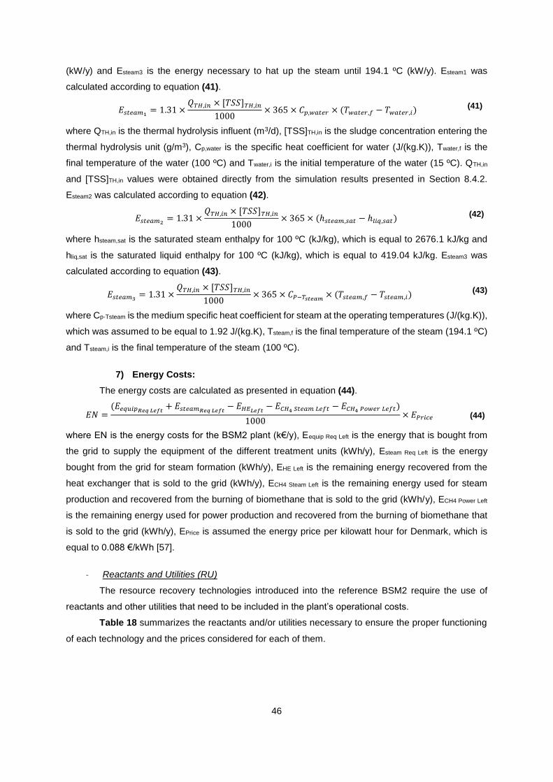
46
(kW/y) and Esteam3 is the energy necessary to hat up the steam until 194.1 ºC (kW/y). Esteam1 was
calculated according to equation (41).
𝐸𝑠𝑡𝑒𝑎𝑚1= 1.31 ×
𝑄𝑇𝐻,𝑖𝑛 × [𝑇𝑆𝑆]𝑇𝐻,𝑖𝑛
1000× 365 × 𝐶𝑝,𝑤𝑎𝑡𝑒𝑟 × (𝑇𝑤𝑎𝑡𝑒𝑟,𝑓 − 𝑇𝑤𝑎𝑡𝑒𝑟,𝑖) (41)
where QTH,in is the thermal hydrolysis influent (m3/d), [TSS]TH,in is the sludge concentration entering the
thermal hydrolysis unit (g/m3), Cp,water is the specific heat coefficient for water (J/(kg.K)), Twater,f is the
final temperature of the water (100 ºC) and Twater,i is the initial temperature of the water (15 ºC). QTH,in
and [TSS]TH,in values were obtained directly from the simulation results presented in Section 8.4.2.
Esteam2 was calculated according to equation (42).
𝐸𝑠𝑡𝑒𝑎𝑚2= 1.31 ×
𝑄𝑇𝐻,𝑖𝑛 × [𝑇𝑆𝑆]𝑇𝐻,𝑖𝑛
1000× 365 × (ℎ𝑠𝑡𝑒𝑎𝑚,𝑠𝑎𝑡 − ℎ𝑙𝑖𝑞,𝑠𝑎𝑡)
(42)
where hsteam,sat is the saturated steam enthalpy for 100 ºC (kJ/kg), which is equal to 2676.1 kJ/kg and
hliq,sat is the saturated liquid enthalpy for 100 ºC (kJ/kg), which is equal to 419.04 kJ/kg. Esteam3 was
calculated according to equation (43).
𝐸𝑠𝑡𝑒𝑎𝑚3= 1.31 ×
𝑄𝑇𝐻,𝑖𝑛 × [𝑇𝑆𝑆]𝑇𝐻,𝑖𝑛
1000× 365 × 𝐶𝑃−𝑇𝑠𝑡𝑒𝑎𝑚
× (𝑇𝑠𝑡𝑒𝑎𝑚,𝑓 − 𝑇𝑠𝑡𝑒𝑎𝑚,𝑖) (43)
where Cp-Tsteam is the medium specific heat coefficient for steam at the operating temperatures (J/(kg.K)),
which was assumed to be equal to 1.92 J/(kg.K), Tsteam,f is the final temperature of the steam (194.1 ºC)
and Tsteam,i is the final temperature of the steam (100 ºC).
7) Energy Costs:
The energy costs are calculated as presented in equation (44).
𝐸𝑁 =(𝐸𝑒𝑞𝑢𝑖𝑝𝑅𝑒𝑞 𝐿𝑒𝑓𝑡
+ 𝐸𝑠𝑡𝑒𝑎𝑚𝑅𝑒𝑞 𝐿𝑒𝑓𝑡− 𝐸𝐻𝐸𝐿𝑒𝑓𝑡
− 𝐸𝐶𝐻4 𝑆𝑡𝑒𝑎𝑚 𝐿𝑒𝑓𝑡 − 𝐸𝐶𝐻4 𝑃𝑜𝑤𝑒𝑟 𝐿𝑒𝑓𝑡)
1000× 𝐸𝑃𝑟𝑖𝑐𝑒 (44)
where EN is the energy costs for the BSM2 plant (k€/y), Eequip Req Left is the energy that is bought from
the grid to supply the equipment of the different treatment units (kWh/y), Esteam Req Left is the energy
bought from the grid for steam formation (kWh/y), EHE Left is the remaining energy recovered from the
heat exchanger that is sold to the grid (kWh/y), ECH4 Steam Left is the remaining energy used for steam
production and recovered from the burning of biomethane that is sold to the grid (kWh/y), ECH4 Power Left
is the remaining energy used for power production and recovered from the burning of biomethane that
is sold to the grid (kWh/y), EPrice is assumed the energy price per kilowatt hour for Denmark, which is
equal to 0.088 €/kWh [57].
- Reactants and Utilities (RU)
The resource recovery technologies introduced into the reference BSM2 require the use of
reactants and other utilities that need to be included in the plant’s operational costs.
Table 18 summarizes the reactants and/or utilities necessary to ensure the proper functioning
of each technology and the prices considered for each of them.

47
Table 18 – Dosages and weighted average prices for the reactants and utilities introduced into the BSM2 (pp –
precipitated).
Technology Utility/
Reactant
Utility/ Reactant
Dosage Source Price
(€/kg)
Weighting
Factor (%)
Weighted
Average
(€/kg)
Supplier
Chemical Precipitation
FeSO4.7H2O 1.8 mol
FeSO4.7H2O : 1 mol PO4
3- pp
[58]
135.50 5
11.14
Sigma-Aldrich 2016
12.33 31.7 Noah Tech. 2016
1.39 31.7 Made-in-China
2016
0.070 31.7 Alibaba 2016
Exelys Technology
Steam 1.31 kg steam: 1 kg dry sludge
treated [22] 0
Produced within the plant
Phosnix Technology
Mg(OH)2 1 mol Mg(OH)2 : 1 mol PO4
3- pp [34]
46.10 5
7.83
Sigma-Aldrich 2016
11.19 47.5 Noah Tech. 2016
0.45 47.5 Alibaba 2016
The reactants and utilities costs are calculated as described below in equation (45).
𝑅𝑈 = 𝑚𝐹𝑒𝑆𝑂4.7𝐻2𝑂 × 𝐹𝑒𝑆𝑂4. 7𝐻2𝑂𝑃𝑟𝑖𝑐𝑒 + 𝑚𝑀𝑔(𝑂𝐻)2× 𝑀𝑔(𝑂𝐻)2𝑃𝑟𝑖𝑐𝑒
(45)
where RU are the overall reactants and utilities costs (k€/y), 𝑚𝐹𝑒𝑆𝑂4.7𝐻2𝑂 is the mass of iron sulphate
required (kg/y), 𝐹𝑒𝑆𝑂4. 7𝐻2𝑂𝑃𝑟𝑖𝑐𝑒 is the iron sulphate’s hepta-hydrate price (€/kg), 𝑚𝑀𝑔(𝑂𝐻)2 is the mass
of magnesium hydroxide required and 𝑀𝑔(𝑂𝐻)2𝑃𝑟𝑖𝑐𝑒 is the magnesium hydroxide price (€/kg). The
mass of iron sulphate hepta-hydrate and magnesium hydroxide precipitated were calculated according
to what is presented in Table 18. The simulation results for the amount of iron phosphate and struvite
precipitated are presented in Section 8.4.2.
3.4.2.2 REVENUE AND OPERATING PROFIT
The weighted commercial value assumed for the iron phosphate and for the struvite is
summarized below in Table 19.

48
Table 19 – Weighted commercial value (€/kg) assumed for each added-value product recovered in the BSM2 plant.
Reactants Price (€/kg) Weighting Factors (%) Weighted Average (€/kg) Source
FePO4
102.50 5
7.77
Sigma-Aldrich 2016
1.75 47.5 Noah Tech. 2016
3.80 47.5 Alibaba 2016
MAP
328 5
16.94
Sigma-Aldrich 2016
0.21 47.5 Nieminen 2010
0.93 47.5 Alibaba 2016
The profit obtained from the chemical precipitation process was calculated according to
equation (46).
𝐶𝑃𝑃𝑟𝑜𝑓𝑖𝑡 =𝑚𝐹𝑒𝑃𝑂4
1000 × 1000× 𝐹𝑒𝑃𝑂4𝑃𝑟𝑖𝑐𝑒
× 365 (46)
where CPProfit is the chemical precipitation profit (k€/y), mFePO4 is the mass of iron phosphate recovered
during the process (g) and FePO4Price is the commercial value of iron phosphate (€/ton). The profit
obtained from the Phosnix technology was calculated according to equation (47).
𝑃ℎ𝑜𝑠𝑛𝑖𝑥𝑃𝑟𝑜𝑓𝑖𝑡 =𝑚𝑀𝐴𝑃
1000 × 1000× 𝑀𝐴𝑃𝑃𝑟𝑖𝑐𝑒 × 365 (47)
where PhosnixProfit is the Phosnix technology profit (k€/y), mMAP is the mass of struvite (MAP) recovered
during the process (g) and MAPPrice is the commercial value of struvite (€/ton).
The revenue for each BSM2 configuration considered is calculated according to equation (48).
𝑅𝑒𝑣𝑒𝑛𝑢𝑒 = 𝐶𝑃𝑃𝑟𝑜𝑓𝑖𝑡 + 𝑃ℎ𝑜𝑠𝑛𝑖𝑥𝑃𝑟𝑜𝑓𝑖𝑡 (48)
where Revenue is the overall profit of the plant (k€/y). The plant’s operating profit (k€/y) is calculated
according to equation (49).
𝑂𝑝𝑒𝑟𝑎𝑡𝑖𝑛𝑔 𝑃𝑟𝑜𝑓𝑖𝑡 = 𝑅𝑒𝑣𝑒𝑛𝑢𝑒 − 𝑂𝐶 (49)
3.5 CHAPTER CONCLUSIONS
The retrofitted BSM2 presented in this chapter aims at maximizing resource recovery in
WWTPS. Different simulation scenarios were generated, which contemplate different combinations of
three full-scale technologies for onsite energy generation, namely the Exelys technology, and for nutrient
recovery, namely the chemical precipitation process and the Phosnix technology.
The reference BSM2 contains a huge level of information that cannot be provided in this thesis,
due to its extension. In this way, further information, related to the technological features included in the
model that are not described above, can be consulted in the following references: [8], [33], [36], [37] and
[43]. The information provided by these articles includes as well the base-equations for calculating the
operating costs of the reference BSM2, considered in the present work. In order to account for the
energetic consumption of the resource recovery technologies introduced into the reference BSM2 and
to calculate the revenue and operating profit for the different simulation scenarios, new equations were
introduced into the model, as aforementioned.

49
4 RESULTS AND DISCUSSION
4.1 GLOBAL MASS BALANCE RESULTS
To assure the correct implementation of each technology a global mass balance was applied to
each BSM2 configuration, considering the phosphorus and nitrogen components. The boundary
considered for the mass balance implementation is represented in Figure 16.
Table 20 summarizes the mass balance results for the base-case scenario, C0. The global mass
balances for the remaining scenarios were implemented in the same way as C0 and are presented in
attachment in Section 8.4.1.
FeSO4.7H2O
Mg(OH)2
Figure 16 – Schematic representation of the boundary established for the implementation of the global mass balance. The boundary
considered in represented in grey.

50
Table 20 – Global mass balance for C0. The column denominated %influent (m/m) calculates the percentage of each output component related to total nitrogen or phosphorus in the influent, depending on the component in question.
In Out
Streams Components Load (kg/d)
Load %(m/m)
Streams Components Load (kg/d)
Load %(m/m)
%influent (m/m)
Infl
uen
t
Soluble P 134.2 77.0
Eff
luen
t
Soluble P 140.0 96.0 80.3
Organic P 40.0 23.0 Organic P 5.8 4.0 3.3
Total P 174.2 100.0 Total P 145.8 100.0 83.7
TKN 1147.0 100.0 TKN 44.3 8.3 3.9
NO3-/NO2
- 0.0 0.0 NO3-/NO2
- 207.6 39.1 18.1
N2 0.0 0.0 N2 279.2 52.6 24.3
Total N 1147.0 100.0 Total N 531.1 100.0 46.3
Slu
dg
e
Soluble P 1.7 6.1 1.0
Organic P 26.7 93.9 15.3
Total P 28.4 100.0 16.3
TKN 193.3 100.0 16.9
NO3-/NO2
- 0.0 0.0 0.0
N2 0.0 0.0 0.0
Total N 193.3 100.0 16.9
N2 Emissions 422.6 36.8
4.2 ECONOMIC EVALUATION RESULTS
The economic evaluation allows to compare the economic performance of the different simulation
scenarios tested. The main features considered during this evaluation are: (a) the operating costs
associated to each scenario, (b) the revenue and (c) the operating profit. The mathematical formulation
used to calculate the operating costs is presented in Section 3.4.2.1, while the equations used to
describe the revenue and operating profit are presented in Section 3.4.2.2. The results obtained for the
economic evaluation are presented in Sections 4.2.1 and 4.2.2.
4.2.1 OPERATING COSTS
As described above in equation (18) (Section 3.4.2.1), the calculation of the operating costs
associated to each simulation scenario studied comprises the following costs: effluent quality costs,
sludge production costs, external carbon source costs, energetic costs and the costs associated with
reactants and utilities. The different costs are presented below.
- Effluent Quality (EQ)
The effluent quality costs calculated for the different simulation scenarios are presented below
in Table 21.

51
Table 21 – Calculation of the pollutant loads for the effluent streams (TSS, COD, TKN, SNO, BOD5, EQI (kg
Pollution Units (PU)/(d))and calculation of the respective effluent quality costs (k€/y).
Scenario
TSS
(kg
PU/d)
COD
(kg
PU/d)
TKN
(kg
PU/d)
SNO
(kg
PU/d)
BOD5
(kg
PU/d)
PTOTAL
(kg
PU/d)
EQI
(kg
PU/d)
EQ
(k€/y)
C0 295.07 989.07 44.29 207.57 47.64 140.00 7488.30 374.41
C1 295.89 989.27 44.32 205.84 47.68 28.00 5232.53 261.63
C2 298.92 1565.18 44.69 210.69 48.08 142.91 8168.82 408.44
C3 295.69 989.02 44.27 205.16 47.62 111.56 6894.68 344.73
C4 298.63 1579.33 44.69 214.35 48.08 28.80 5937.40 296.87
C5 295.85 989.22 44.30 203.46 47.67 22.30 5094.03 254.70
C6 298.88 1565.14 44.66 208.27 48.07 22.55 5736.40 288.82
C7 298.88 1201.76 44.68 210.14 48.08 112.82 7197.79 359.89
From Table 21 it is possible to understand that simulation scenario C2 presents the highest
effluent quality costs, opposed to scenario C5, which presents the lowest costs, followed by scenarios
C1 and C6 (in increasing order). The simulation scenarios C3, C7 and C0 (in increasing order) have
intermediate costs.
Scenario C2 is generated by introducing the Exelys technology in the BSM2 layout. As explained
above in Section 3.3.2, the Exelys technology is a thermal hydrolysis process, which comprises a COD
solubilisation step [22] and results in an increase of the soluble components and a decrease of the
particulate fraction in the influent stream to the anaerobic digester. As shown in Figure 11, the stream
recycled back from the thermal hydrolysis into the main treatment line is the overflow from the
dewatering unit, which is a liquid stream. This way, the introduction of the Exelys technology into the
BSM2 results in a higher soluble content present in the stream recycled back to the main process, which
in turn increases the loads of soluble pollutants present in the stream (especially COD, nitrates and
nitrites, and phosphorus) and, consequently, the costs associated with the effluent quality.
The simulation scenario C5 involves the addition of the chemical precipitation process, and of
the Phosnix technology to the default BSM2. Both technologies remove the soluble phosphorus from
different streams: the chemical precipitation from the secondary clarifier effluent and the Phosnix
treatment from the reject water from the dewatering unit. This last technology also removes ammonium,
as described in Sections 3.3.1 and 3.3.3, respectively. Thus, as a result from the combination of these
two treatment units, the amount of pollutants in the effluent is drastically reduced and, consequently,
the costs related to the effluent quality are lower.
The simulation scenario C1 presents the second lower effluent quality costs, which is due to the
fact that it corresponds only to the introduction of the chemical precipitation process in the BSM2 and
leads to a lower pollutant removal and higher effluent quality costs compared to C5.
The simulation scenario C6 is the third scenario with lower effluent quality costs, because it
comprises the introduction of the Exelys and the Phosnix technologies. The Phosnix technology intends
to remove the soluble phosphorus and ammonia present in the overflow stream of the dewatering unit
(Figure 12), through struvite precipitation. Since the Phosnix efficiency is set to remove 83% of the

52
soluble phosphorus content of the stream and a corresponding stoichiometric amount of ammonium in
a proportion of 1 to 1, as presented in the section 3.3.3, the Phosnix technologies smoothes the increase
of charge of pollutants due to the implementation of the Exelys technology.
The simulation scenarios C3, C7 and C0 (in increasing order) present intermediate effluent quality
costs, when considering the costs associated with the scenarios C5 and C2, the less and most expensive
scenarios, respectively. Scenario C3 refers to the introduction of the mere Phosnix technology into the
BSM2. As stated above, the introduction of the Phosnix technology reduces the pollutant load that is
recycled back to the main treatment and, consequently, reduces the pollutant load in the effluent stream.
However, C3 presents, approximately, a 35% increase of the effluent quality costs compared to C5,
which is related to the fact that the influent flow rate to the Phosnix technology is two orders of magnitude
lower than the influent flowrate to the chemical precipitation process, leading to a smaller removal of
pollutants by the Phosnix technology. The same is verified for scenario C7, which presents effluent
quality costs slightly higher than scenario C3, because this scenario includes not only the addition of the
Phosnix technology, but also the Exelys technology as well to the reference BSM2. As previously
concluded, the Exelys technology results in an increase of the effluent quality costs of the scenario in
question.
With regards to the simulation scenario C0, it presents effluent quality costs higher than both C3
and C7 because it does not include any technology that reduces the pollutant load of the plant, however,
not having the Exelys technology, which increases the pollutant load of the plant, allows C0 to have
lower effluent quality costs than scenario C2.
In conclusion, it has been observed that both the chemical precipitation and the Phosnix
technologies have the potentiality of reducing the effluent quality costs and, consequently, the operating
costs of the plant related to the violations of effluent law limit. On the other hand, the Exelys technology
has been found to increase the pollutant load of the plant and the effluent quality costs.
- Sludge Production (SP)
The costs associated with sludge production are summarized below in Table 22.
Table 22 – Sludge production (kg/y) and sludge production associated costs (k€/y).
Scenario SP (kg/y) SP (k€/y)
C0 8.66×10⁵ 177.90
C1 8.66×10⁵ 177.96
C2 6.27×10⁵ 128.88
C3 8.66×10⁵ 177.88
C4 6.38×10⁵ 131.12
C5 8.66×10⁵ 177.95
C6 6.27×10⁵ 128.87
C7 6.06×10⁵ 124,60
As can be observed in Table 22, the simulation scenarios studied can be divided in two groups
with regards to the sludge production costs: one comprises simulation scenarios C0, C1, C3 and C5 and

53
the other comprises scenarios C2, C4, C6 and C7. As can be noted, the former present approximately
30% higher sludge production costs than the latter.
From Table 16 it is possible to understand that all the simulation scenarios with lower sludge
production costs include the Exelys technology. Once that the sludge production costs are directly
proportional to the load of sludge produced, as explained by equation (26), it is understandable that the
lower sludge production costs for scenarios that include the Exelys technology are due to the fact that
this technology decreases the amount of sludge produced thanks to the higher solubilisations of
wastage sludge. And this in turn, reduces the costs related to it.
From the previous analysis, it can be understood that the Exelys technology impacts negatively
the sludge production costs, by decreasing them. Furthermore, is can also be concluded that the
chemical precipitation and the Phosnix technologies do not affect the sludge production, which makes
sense because these two technologies intend to precipitate soluble components present in liquid
streams of the WWTP, opposed to the Exelys technology which acts upon the particulate fraction of the
underflow streams of the plan.
- External Carbon (EC)
The external carbon source costs are summarized below in Table 23.
Table 23 – External carbon source (kg/y) and associated costs (k€/y).
Scenario EC (kg/y) EC (k€/y)
C0 2.92×10⁵ 60.00
C1 2.92×10⁵ 60.00
C2 2.92×10⁵ 60.00
C3 2.92×10⁵ 60.00
C4 2.92×10⁵ 60.00
C5 2.92×10⁵ 60.00
C6 2.92×10⁵ 60.00
C7 2.92×10⁵ 60.00
The costs associated with the addition of an external carbon source to the plant do not vary for
the different simulation scenarios tested, as presented in Table 23. This happens because the external
carbon source is an input to the BSM2, being already part of the operating costs of the BSM2 base-
case scenario, C0. It is added to the WWTP at a fixed flow rate and fixed concentration, as presented in
Section 3.4.2.1, resulting in a fixed operating cost of the plant.
- Energy (EN)
Electricity can be either bought from the grid, to ensure that there is enough energy to cover the
energetic demands of the WWTP, or sold to the grid, if there is internal production of energy within the
plant is sufficient so satisfy the plant energy requirements. Consequently, the energy included in the
operating costs of the plant can have a positive or negative value, whether it is bought or sold,
respectively.

54
A) BSM2 Energy Consumption
The energy consumptions are summarized in Table 24.
Table 24 – Energy consumption for BSM2 base-case configuration (AE, PE, MEAS, MEAD, ME, EBSM2 Base-case)
(kWh/y).
Scenario AE
(kWh/y)
PE
(kWh/y)
MEAS
(kWh/y)
MEAD
(kWh/y)
ME
(kWh/y)
EBSM2 Base-case
(kWh/y)
C0 1.28×10⁶ 1.61×10⁵ 1.31×10⁵ 1.49×10⁵ 2.80×10⁵ 1.72×10⁶
Table 24 presents the energy consumed for the BSM2 base-case plant, which is equal for all
the different simulation scenarios tested.
The aeration energy, calculated according to equation (28), depends on the volume of the
activated sludge tank, on the saturation oxygen concentration and on the liquid oxygen concentration in
the tank and on the oxygen mass transfer coefficient. Among these, the only factor which can change
is the oxygen concentration. Taking this into account, it can be concluded that the introduction of the
resource recovery technologies does not affect considerably the biomass activity in the activated sludge
unit; otherwise, the oxygen concentration in the activated sludge reactors would have varied, thus
leading to remarkably-different aeration energy consumes.
With regards to the pumping energy, which is the energy necessary for pumping sludge
streams along the plant, this only depends on the flow rates of the underflow streams present in the
plant, as included in equation (29), namely activated sludge internal recycle stream, primary underflow
stream, secondary settler recycle underflow stream, secondary settler wastage underflow stream,
thickener underflow stream, Exelys technology effluent stream (for the simulation scenarios that
contemplate the Exelys technology) and the dewatering unit overflow stream. All the flow rates of the
streams mentioned above are fixed inputs of the BSM2, with the exception of the Exelys effluent stream,
which was introduced into the pumping energy equation in order to adapt it to the extended BSM2. The
additional underflow stream increases the pumping energy consumptions of the simulation scenarios
C2, C4, C6 and C7 by approximately564 kWh/y, which has no expression in the overall pumping energy
of these combinations, resulting in a constant pumping energy consumption for all the scenarios.
The mixing energy is calculated as described in equations (30) to (32), depending only on the
volume of the activated sludge reactors and on the volume of the anaerobic digester, which are fixed
inputs of the model, as stated above in sections 3.1.1 and 3.1.2. This way, the mixing energy is constant
for all the simulation scenarios analysed, independently of the introduction of the resource recovery
technologies in the BSM2 model.
In conclusion, the energy consumed by the reference BSM2 plant is the same for every
simulation scenario tested.
B) Energy Consumption of the Resource Recovery Technologies
To be able to quantify the energy consumption of the equipment newly introduced in the different
BSM2 simulation scenarios studied, it is first necessary to size the equipment. The equipment sizing
was performed as presented in Section 3.4.2.1, Table 25 presents the ideal dimensions identified for
the different treatment units for each simulation scenario.

55
Table 25 - Equipment dimensions for each BSM2 scenario.
Scenario VMixer (m3) VFlocculator (m3) VExelys Reactor (m3) VPhosnix Reactor (m3)
C0 --- --- --- ---
C1 3.59 344.20 --- ---
C2 --- --- 0.67 ---
C3 --- --- --- 7.84
C4 3.59 344.20 0.67 ---
C5 3.59 344.20 --- 7.85
C6 3.59 344.20 0.67 1.91
C7 --- --- 0.67 1.92
From Table 25 it is possible to understand that the mixer volume is two orders of magnitude
lower than the flocculator volume (both units from the chemical precipitation process). The volume of
the two units is calculated according to equation (33) and depends on the influent flow rate to the unit,
which is the same for both units, and on the detention time of each unit. The flocculator has a detention
time of 1200 seconds and the mixer has a detention time of 12.5 seconds, which explains the increased
volume of the flocculator, when compared against the one of the mixer.
The Exelys reactor volume was calculated according to equation (34) and its low value is
explained by the very small retention time of the process (30 minutes), as explained in Section 3.3.2.
The Exelys reactor has the same volume for every simulation scenario because the flow rate to the
Exelys technology is fixed (sum of the primary and thickener underflow streams).
The lower volume of the Phosnix reactor for the simulation scenarios C6 and C7, when compared
to scenarios C3 and C5, is related to the introduction of the Exelys technology into these scenarios. As
explained above in Section 3.3.2, the influent sludge to the Exelys technology has a fixed concentration
of dry sludge (DS), specifically the sludge enters the Exelys reactor at 24.2% DS. A dewatering unit was
introduced into the model on top of the Exelys technology, in order to concentrate the sludge at desired
concentration. The reject water from this dewatering unit is recycled back to the beginning of the
treatment, not being part of the influent of the Phosnix technology. As explained in Section 3.4.2.1, the
volume of the Phosnix reactor is established based on the influent flow rate to the technology; in this
way, having a smaller influent flow rate for the scenarios C6 and C7 leads to a decrease in the Phosnix
reactor volume for these scenarios.
Once the dimensions of the pieces of equipment introduced in each one of the simulation
scenarios studied are known, it is possible to determine the respective power requirements, which are
summarized in Table 26.

56
Table 26 – Power requirements (kWh/y) for the pieces of equipment present in each configuration of BSM2. Legend:
MixerE, FloccE, ExelysE, PhosnixE- equipment energy requirements for the mixer and the flocculator (chemical precipitation), and for the Exelys and Phosnix technologies, respectively. EBSM2 extended – overall equipment energy requirements for the resource recovery technologies.
Scenario MixerE
(kWh/y) FloccE(kWh/y)
ExelysE (kWh/y)
PhosnixE (kWh/y)
EBSM2 extended
(kWh/y)
C0 --- --- --- --- ---
C1 2.77×10⁴ 7.11×10³ --- --- 2.98×10⁴
C2 --- --- 1.40×10³ --- 1.40×10³
C3 --- --- --- 2.55×10⁵ 2.55×10⁵
C4 2.77×10⁴ 7.11×10³ 1.40×10³ --- 3.12×10⁴
C5 2.77×10⁴ 7.11×10³ --- 2.55×10⁵ 2.85×10⁵
C6 2.77×10⁴ 7.11×10³ 1.40×10³ 6.23×10⁴ 9.35×10⁴
C7 --- --- 1.40×10³ 6.06×10⁴ 6.40×10⁴
As can be seen in Table 26, the power requirement of the mixer unit is always bigger than the
power requirement of the flocculator unit, which contrasts with the volume relationship between the two
units. As demonstrated in equation (34), the power requirements of these units depend on the volume
and on the square of the required velocity gradient of each unit. Due to this, this last parameter has a
greater influence in the power requirement calculation than the volume. This means that, even though
the volume of the flocculator is two orders of magnitude bigger than the mixer’s volume, the power
requirement of the mixer is higher because the velocity gradient for this unit is bigger than the velocity
gradient of the flocculator (875 s-2 and 50 s-2, respectively).
The equipment energy requirements of the Exelys technology include the energy spent in order
to provide appropriate mixing for the reactor. This technology presents the lowest energy requirements,
when compared to the energy requirements of the equipment of other technologies, which is in
agreement with the reduced volume of the Exelys reactor, as can be observed in Table 25. Furthermore,
the Exelys energy requirements are constant for every scenario because the mixing energy is calculated
based on the sludge volume admitted to the reactor. Considering that the influent stream has a fixed
flow rate and fixed sludge concentration, the sludge volume admitted to the reactor does not vary.
In contrast, from Table 26, it is possible to understand that the Phosnix technology has the
highest power requirements of all the resource technologies considered. The power requirements of the
Phosnix reactor were calculated according to equation (36) and the high energy consumptions
associated to this reactor can be explained by the fact that this is an air-lift reactor, which requires the
need for constant sparging in order to maintain the fluid circulation inside the reactor and to promote
homogenization.
Considering the sum of the energetic requirements of the different resource recovery
technologies integrated in each simulation scenario presented in Table 26, it is understood that scenario
C2 presents the lowest energy requirements and the scenario C5 presents the highest ones. Scenario
C2 has the lowest power requirements since it only comprises the addition of the Exelys technology to
the BSM2 and because the Exelys technology is the technology that consumes less energy, as
explained above.

57
On the other hand and according to Table 26, the scenario with highest power requirements is
the scenario C5, even though it was expected to be scenario C6. The scenario C6 was expected to
require the most amount of energy because it includes the three additional technologies into the BSM2
(opposed to scenario C5 which only includes the chemical precipitation process and the Phosnix
technology). However, this hypothesis was not verified because the power requirements of the Phosnix
reactor for scenario C6 are approximately 75% lower than the power requirements of the Phosnix reactor
for scenario C5. The reduction in the Phosnix reactor power requirements for scenario C6 is related with
the reduction of the Phosnix influent flow rate for this scenario, which is associated with the introduction
of the Exelys technology. As explained above, the Exelys technology decreases the Phosnix’s influent
flow rate, consequently leading to a reduction of the Phosnix reactor volume and to a reduction of the
reactor power requirements, resulting in overall lower power requirements for scenario C6. The total
energy consumed by the equipment present in each simulation scenario is presented below in Table
27.
Table 27 – Total energy consumed by the equipment for the different simulation scenarios tested. Legend: EBSM2 –
equipment energy requirements from the reference BSM2 (are the same for every scenario); EBSM2 extended – equipment energy requirements of the chemical precipitation, the Exelys and the Phosnix technologies all together; Eequipment – is the sum of EBSM2 Base-case and EBSM2 extended (see also equation (37)).
Scenario EBSM2 Base-case
(kWh/y)
EBSM2 extended
(kWh/y) Eequipment (kWh/y)
C0 1.72×10⁶ --- 1.72×10⁶
C1 1.72×10⁶ 2.98×10⁴ 1.75×10⁶
C2 1.72×10⁶ 1.40×10³ 1.72×10⁶
C3 1.72×10⁶ 2.55×10⁵ 1.97×10⁶
C4 1.72×10⁶ 3.12×10⁴ 1.75×10⁶
C5 1.72×10⁶ 2.85×10⁵ 2.00×10⁶
C6 1.72×10⁶ 9.35×10⁴ 1.82×10⁶
C7 1.72×10⁶ 6.40×10⁴ 1.79×10⁶
Table 27 shows that the energetic requirements associated with the introduction of the resource
recovery technologies into the BSM2 are 1 to 3 orders of magnitude lower than the energetic
requirements of the reference BSM2, not having a strong impact on the plant’s overall equipment
energetic requirements; only scenarios C5, C3, C6 and C7 present an increase in the overall energetic
requirements. In concordance to what was concluded above, these scenarios correspond to the
simulation scenarios that include the Phosnix technology, which is the resource recovery technology
with highest equipment power requirements.
Overall, it has been proven that the Exelys technology leads to the lowest power requirements
while the Phosnix technology leads to the highest energetic demand.

58
C) Energy Recovered from the BSM2 Plant
It was considered that from the burning of the biomethane, 30% of the energetic content of the
biomethane is lost as heat. Of the remaining 70%, 50% is used for power production (equipment supply)
and the remainder is used for steam production.
Table 28 summarizes the energy recovered from the BMS2. More specifically, the table reports the
energy recovered as heat from the Exelys technology and the energy produced through biogas
conversion, for the different simulation scenarios studied.
Table 28 – Energy recovered from the BSM2 plant (EHE, ECH4, ECH4 Steam and ECH4 Power (kWh/y)) and energy
consumed by the Exelys technology (Esteam (kWh/y)) for the different BSM2 configurations.
Scenario EHE
(kWh/y)
ECH4
(kWh/y)
ECH4 Steam
(kWh/y)
ECH4 Power
(kWh/y)
C0 --- 4.59×10⁶ --- 4.59×10⁶
C1 --- 4.94×10⁶ --- 4.93×10⁶
C2 1.48×10⁶ 5.13×10⁶ 2.57×10⁶ 2.57×10⁶
C3 --- 4.94×10⁶ --- 4.94×10⁶
C4 1.45×10⁶ 5.10×10⁶ 2.55×10⁶ 2.55×10⁶
C5 --- 4.93×10⁶ --- 4.93×10⁶
C6 1.45×10⁶ 5.13×10⁶ 2.57×10⁶ 2.57×10⁶
C7 1.45×10⁶ 4.33×10⁶ 2.16×10⁶ 2.16×10⁶
From Table 28 it can be observed that the energy recovered from the heat exchanger of the
Exelys technology does not vary significantly from one scenarios to another. As described in equation
(38), the energy recovered from the heat exchanger in the Exelys technology depends on the flow rate
of the thermal hydrolysis effluent. Once that the Exelys flow rate is fixed, as explained above, then the
corresponding energy recovered from the heat exchanger is approximately constant for every scenario.
Regarding the energy recovered from the biomethane conversion (ECH4), it can be observed in
Table 28, that the simulation scenarios C2, C4 and C6 present the highest energy values, having an
average increase of approximately 11,5%, when compared to the energy recovered from the
biomethane conversion of the base-case scenario, C0. From Table 16, is understood that these
simulation scenarios correspond to the scenarios that include the Exelys technology since the
technology solubilizes organic matter and thus increases its conversion rate into biogas in the
subsequent digestion unit. However, the scenario C7, which also includes the Exelys technology, has
the lowest amount of energy recovered from the biomethane conversion, reflecting, approximately, a
15,4% decrease when compared to the average results for the other simulation scenarios that include
the Exelys technology. This outcome can be explained by the conversion rate of the methane considered
in the ADM1, presented previously in Table 14. More specifically, According to the ADM1 [45], biogas
production depends mainly on acetate and hydrogen uptake rates, as can be seen in Table 14, and it
is modelled according to equation (50).
𝑆𝐶𝐻4= (1 − 𝑌𝑎𝑐) × 𝑘𝑚,𝑎𝑐
𝑆𝑎𝑐
𝑘𝑆 + 𝑆𝑎𝑐
𝑋𝑎𝑐𝐼3 + (1 − 𝑌ℎ2) × 𝑘𝑚,ℎ2
𝑆ℎ2
𝑘𝑆 + 𝑆ℎ2
𝑋ℎ2𝐼1 (50)
where SCH4 is the methane gas concentration (kg COD/m3), Yac is of biomass on acetate yield (kg
COD_X.kg COD_S), km,ac is the specified Monod maximum uptake rate for acetate (kg COD.m-3_S.kg

59
COD.m-3_X.d-1), Sac is total acetate (kg COD/m3), KS is the Monod half saturation constant (kg COD/m3),
Xac are the acetate degraders (kg COD/m3), I3 is an inhibition factor (dimensionless), Yh2 is the biomass
on hydrogen yield (kg COD_X.kg COD_S), km,h2 is the specified Monod maximum uptake rate for
hydrogen (kg COD.m-3_S.kg COD.m-3_X.d-1), Sh2 is the hydrogen gas (kg COD/m3), Xh2 are the
hydrogen degraders (kg COD/m3) and I1 is an inhibition factor (dimensionless).
However, the methane conversion rate is dependent on two inhibition factors as well, as
described in equation (50), namely I3 and I1. The inhibition factor I3 is modelled according to the following
equation, equation (51).
𝐼3 = 𝐼𝑝𝐻 × 𝐼𝐼𝑁 𝑙𝑖𝑚 × 𝐼𝑁𝐻3,𝑋𝑎𝑐 (51)
where IpH is the pH inhibition factor, IIN lim is the inorganic nitrogen inhibition due to substrate limitation
and INH3, Xac is the free ammonia inhibition due to non-competitive inhibition. And the inhibition factor I1
is modelled according to equation (52).
𝐼1 = 𝐼𝑝𝐻 × 𝐼𝐼𝑁 𝑙𝑖𝑚 (52)
where SNH3 is the free ammonia (kg COD/m3) and K I NH3 is the free ammonia inhibition constant (kg
COD/m3).
The low energy recovery observed for scenario C7 can be associated with the fact that the
introduction of the Exelys and the Phosnix technologies by themselves, without the chemical
precipitation process, results in a higher soluble phosphorus concentration in the overall plant, which
leads to a higher amount phosphorus precipitated as struvite in the Phosnix process. Taking into
consideration the struvite composition (MgNH4PO4.6H2O), it can be understood that higher amounts of
phosphorus precipitated in the form of struvite lead to higher amounts of ammonium precipitated as well
(1 mol:1 mol ratio). This increase in the amount of ammonium precipitated decreases the amount of
biomass generated in the activated sludge unit and thus the amount of biomass which can be possibly
solubilised and subsequently converted into methane.
Overall, the main conclusion to draw from Table 28 is that the Exelys technology performance
fell short compared to the expectations. It was expected that the electricity production would be
increased, approximately, by 20%, as reported by Carrère et al. (2010),and Gurieff et al. (2011), while
it increased of only 11,5%. This outcome can be explained by the fact that the ADM1 model has not
been subject to further developments after its creation and the modelling used may not be shaped to
integrate a process such as the Exelys technology.
The free ammonia inhibition is modelled according to equation (53).
𝐼𝑁𝐻3,𝑋𝑎𝑐=
1
1 +𝑆𝑁𝐻3
𝐾𝐼 𝑁𝐻3
(53)
where SNH3 is the free ammonia (kg COD/m3) and K I NH3 is the free ammonia inhibition constant (kg
COD/m3).
The introduction of the Exelys technology into the BSM2 increased significantly the free ammonia
present in the anaerobic digestion influent, due to the higher degree of biomass solubilisation. The

60
increase in SNH3 decreases the value of INH3, Xac, decreasing in turn I3 and, consequently, decreasing the
acetate uptake rate and Sch4, preventing the increase in biogas production.
D) Energy Consumed for Steam Production in the BSM2 Plant
The steam production within the BSM2 is accomplished through the use of an electrical steam boiler.
The energy input to the boiler is assured by the electricity generated in the CHP system, in the first
place. If the energy recovered from the heat exchanger is lower than the energy required for the steam
production, then the steam production is accomplished by using the electricity generated from
biomethane, which is produced during the anaerobic digestion. However, if the electricity recovered
from the biomethane conversion is not sufficient to ensure the required steam production for the thermal
hydrolysis process, the remaining electricity required is bought from the grid.
Table 29 summarizes the energy required for steam production for the different simulation
scenarios considered.
Table 29 – Energy consumed for production of the steam used in the Exelys technology.
Scenario Esteam 1 (kW/y) Esteam 2 (kW/y) Esteam 3 (kW/y) Esteam (kWh/y)
C0 --- --- --- ---
C1 --- --- --- ---
C2 1.00×10⁹ 6.39×10⁹ 5.08×10⁸ 2.19×10⁶
C3 --- --- --- ---
C4 1.00×10⁹ 6.39×10⁹ 5.08×10⁸ 2.19×10⁶
C5 --- --- --- ---
C6 1.00×10⁹ 6.39×10⁹ 5.08×10⁸ 2.19×10⁶
C7 1.00×10⁹ 6.39×10⁹ 5.08×10⁸ 2.19×10⁶
The energy required for steam production is constant for all scenarios because, as previously
discussed, the influent’s flow rate of the Exelys technology is fixed.
E) Energy Net balance and Energy Costs
It was considered that the electricity bought from the grid is accounted as an additional cost in the
operating costs equation (positive term), as shown in equation (18). On the other hand, if the electricity
recovered from the heat exchanger and/or the electricity generated from burning the methane destined
for steam production are higher than the electricity required for the steam production, the remaining
electricity is sold to the grid and is accounted in the operating costs as a saving (negative term).
Table 30 presents the energy consumption within the BSM2 plant for each simulation scenario
studied.

61
Table 30 – Energy consumption required left by the BSM2 plant after the consumption of the renewable plant and
remaining renewable energy produced by the plant that was not consumed (kWh/y). Energy (EN) costs (+) and/or savings/profit (-) for the different configurations of the BSM2 plant (k€/y).
Scenario
EEquipment
Required Left
(kWh/y)
ESteam
Required Left
(kWh/y)
EHE Left
(kWh/y)
ECH4 Steam Left
(kWh/y)
ECH4 Power Left
(kWh/y)
EN
(k€/y)
C0 0 --- --- --- 2.87×10⁶ -252.83
C1 0 --- --- --- 3.18×10⁶ -279.72
C2 0 0 0 1.86×10⁶ 8.43×10⁵ -237.85
C3 0 --- --- --- 2.96×10⁶ -260.84
C4 0 0 0 1.81×10⁶ 7.96×10⁵ -229.25
C5 0 --- --- --- 2.92×10⁶ -257.24
C6 0 0 0 1.83×10⁶ 7.51×10⁵ -226.90
C7 0 0 0 1.43×10⁶ 3.78×10⁵ -158.83
Table 30 shows that all the energy consumed in the BSM2 is supplied by the energy recovered
in the plant itself, since EEquipment and Esteam, representing the total energy consumptions of the plant, are
equal to zero for every scenario tested (no energy is bought from the grid). There is also no energy left
from the energy recovered from the heat exchanger that is part of the Exelys technology for all the
scenarios studied, which implies that energy (EHE Left) does not cover the boiler energy requirements to
produce the required amount of steam. However, it is possible to observe that there is still energy for
steam production left from the biomethane (ECH4 Steam Left), meaning that not all the methane energy
available for steam production (ECH4 steam) is consumed.
With regards to the overall energy costs (EN), scenarios C7, C6, C4 and C2, which correspond
to the alternatives that include the Exelys technology, present an average 15% decrease in the energy
savings, when compared to the base-case scenario, C0. This result is a consequence of the low increase
in the biogas production of the simulation scenarios that include the Exelys technology, as previously
explained. Furthermore, the assumption of utilizing the energy recovered within the plant to produce the
required steam for the Exelys technology increases greatly the energetic demand of the scenarios that
include this technology, as can be observed in Table 29, contributing as well for the lower energy
savings associated with these scenarios.
The remaining simulation scenarios present overall energy costs similar to the base-case
scenario, C0, which implies that the chemical precipitation process and the Phosnix technology do not
have a significant energy impact on the overall plant energy consumption.
- Reactants and Utilities Costs (RU)
The reactants used in the different simulation scenarios are iron sulphate hepta-hydrate to
precipitate iron phosphate, in the chemical precipitation process, and magnesium hydroxide to
precipitate struvite, in the Phosnix technology. The annual spendings on these reactants are
summarized in Table 31.

62
Table 31 – Soluble phosphorus precipitated by the chemical precipitation (SPO4-P,pp-CP) and the Phosnix technology
(SPO4-P,pp-Phosnix) (kg PO43-/y). FeSO4.7H2O and Mg(OH)2 costs for each configuration (k€/y).
Scenario SPO4-P,pp-CP
(kg PO43-/y)
FeSO4.7H2O
(kg/d)
FeSO4.7H2O
(k€/y)
SPO4-Ppp-
Phosnix
(kg PO43-/y)
Mg(OH)2
(kg/d)
Mg(OH)2
(k€/y) RU (k€/y)
C0 --- --- --- --- --- --- ---
C1 4.09×10⁴ 2.40×10⁶ 2397.66 --- --- --- 2397.66
C2 --- --- --- --- --- --- ---
C3 --- --- --- 1.04×10⁴ 5756.82 45.08 45.08
C4 4.20×10⁴ 2.47×10⁶ 2466.23 --- --- --- 2466.23
C5 3.26×10⁴ 1.85×10⁶ 1851.51 1.04×10⁴ 5763.90 45.13 1896.64
C6 3.29×10⁴ 1.93×10⁶ 1931.44 1.10×10⁴ 6103.83 47.97 1979.23
C7 --- --- --- 1.11×10⁴ 6176.64 48.37 48.73
From Table 31, it can be observed that the iron sulphate expenses are approximately 25% lower
for scenarios C5 and C6 compared to scenarios C1 and C4. Scenarios C5 and C6 have lower iron sulphate
costs because they include not only the chemical precipitation process but also the Phosnix technology.
The Phosnix technology precipitates 83% of the soluble phosphorus that comes from the underflow
stream of the dewatering unit and, this way, a lower amount of phosphorus is found in the mainstream,
which in turn reduces the amount of iron sulphate required for its precipitation.
With regards to the magnesium hydroxide, it can be understood that there is an increase of
approximately 7% in the magnesium hydroxide expenses for the scenarios C6 and C7, when compared
against scenarios C3 and C7. This increase is related to the introduction of the Exelys technology in
these scenarios. The solubilisation process of the Exelys technology increases the load of soluble
phosphorus available in the plant, which leads to higher phosphorus precipitated in the plant and,
therefore, higher magnesium hydroxide requirements.
Eventually, it is understandable that the overall reactant costs are mainly due to the costs spent on the
reactant for the chemical precipitation process while little is the contribution by the Phosnix technology.
This divergence can be explained, not only by the fact that there is much more phosphorus to precipitate
in the main stream (chemical precipitation), than in the side stream (Phosnix technology), as presented
in by columns SPpp-CP and SP-pp Phosnix, respectively, but also because that the reactant used in the
chemical precipitation profit is, approximately, 42% more expensive than the reactant used in the
Phosnix technology (see Section 3.4.2.1-Table 18).
- Operating Costs of the Plant
The operating costs for the different BSM2 simulation scenarios considered are summarized
next in Table 32.

63
Table 32 – EQ, SP, EC, EN, RU and OC costs (k€/y) for each BSM2 combination considered.
Scenario EQ (k€/y) SP (k€/y) EC (k€/y) EN (k€/y) RU (k€/y) OC (k€/y)
C0 374.41 177.90 60.00 -252.83 0 359.48
C1 261.63 177.96 60.00 -279.72 2397.66 2617.53
C2 408.44 128.88 60.00 -237.85 0 359.47
C3 344.73 177.88 60.00 -260.84 45.08 366.86
C4 296.87 131.12 60.00 -229.25 2466.23 2724.98
C5 254.70 177.95 60.00 -257.24 1896.64 2132.05
C6 288.82 128.87 60.00 -226.90 1979.23 2228.02
C7 359.89 124.60 60.00 -158.83 48.73 434.02
The main observations to be drawn from Table 32 are that, apart from the operating costs of
the simulation scenarios that include the chemical precipitation process, namely scenarios C1, C4, C5
and C6, the scenario that presents the highest operating cost variation when compared to the operating
costs of the base-case scenario - C0 -, is scenario C7 which has approximately a 21% variation when
compared to scenario C0. Scenarios C2 and C3 do not present a significant variation when compared to
the base-case results.
The results obtained for the operating cost of scenario C7 are mainly due to the fact that this
scenario has, approximately, 37% less energy savings than the base-case scenario. This behaviour is
a consequence of a 15,4% less biogas production, as can explained above in Table 28.
The non-significant variation of the operating costs of the scenarios C2 and C3 reflect that the
introduction of the Exelys technology and the Phosnix technology by themselves do not affect the overall
operating costs of the BSM2.
Regarding the results obtained for the operating cost of the simulation scenarios that include
the chemical precipitation process, namely scenarios C1, C4, C5 and C6, these are directly related to the
reactant costs associated with these scenarios, as explained in Table 31.
4.2.2 REVENUE AND OPERATING PROFIT
The introduction of the new treatment units into the BSM2 enabled the recovery of added-value
products. The chemical precipitation process enables the recovery of iron phosphate while the Phosnix
technology allows for the recovery of struvite (MAP). Both products have commercial value and can be
therefore sold and accounted as profit for the BSM2.
Table 33 summarizes the revenue margins obtained for each individual full-scale technology,
as well as the overall operating costs and the revenue margins and the operating profit for each
simulation scenario studied.

64
Table 33 – Chemical precipitation, Phosnix and revenues and operating profit for each BSM2 configuration (k€/y).
Scenario
Chemical
Precipitation Profit
(k€/y)
Phosnix
Profit
(k€/y)
Revenue
(k€/y) OC (k€/y)
Operating
profit
(k€/y)
C0 --- --- --- 359.48 -359.48
C1 503.48 --- 503.48 2617.53 -2114.05
C2 --- --- --- 359.47 -359.47
C3 --- 454.17 454.17 366.86 87.32
C4 517.88 --- 517.88 2724.98 -2207.10
C5 401.06 454.73 855.79 2132.05 -1276.26
C6 405.58 481.55 887.13 2228.02 -1340.89
C7 --- 487.30 487.30 434.02 53.27
One of the main conclusions to be drawn from the overall economic evaluation presented in Table
33 is that the chemical precipitation and the Phosnix profits are of the same order of magnitude.
However, in those scenarios where the chemical precipitation is adopted, operating costs result much
higher than the revenues obtained, thus leading to a drastically-negative operating profit. This result can
be ascribed to the fact that the iron sulphate price used in this work (see Table 18) is, approximately,
43% higher than the commercial value assumed for the iron phosphate (see Table 19).
A clear example demonstrating that the chemical precipitation profit is the technology drastically
reducing the operating profit is scenario C6, where the three resource recovery technologies are
included, which presents the highest revenue margin, yielding 887,13 k€ per year of profit. This scenario
was expected to correspond to the most profitable alternative for the BSM2 plant; however, even though
this scenario has the highest revenue margin, as presented in Table 33, it does not yield to the highest
operating profit because of the high operating costs associated with the chemical precipitation process.
Regarding the remaining scenarios, more specifically scenarios C0, C2, C3 and C7, firstly it can be
observed that scenario C0 presents no revenue margin, because it corresponds to the reference BSM2
scenario, in which no techniques for recovery of added-value products are implemented. Secondly, the
scenario C2 does not present revenue margins, as well. This is because this scenario corresponds to
the introduction of the Exelys technology in the BSM2 plant by itself and, as explained previously, the
additional biogas production associated with the introduction of this technology in the BSM2 and the
consequent additional energy generation are taken into account in the energy costs/savings of the plant,
and not as revenue. Furthermore, scenario C2 presents an operating profit equal to the one presented
by the base-case scenario C0, implying that despite the verified low increase in the biogas production
for the scenarios that include the Exelys technology, in an overall context, the introduction of this
technology into the BSM2 does not impact negatively the plant retrofitting.
Lastly, the scenarios C3 and C7, despite having the lowest revenue margins of all the simulation
scenarios studied, present, not only the highest operating profit values, but also positive operating
profits. The simulation scenario C3, which corresponds to the introduction of the Phosnix technology by
itself into the BSM2 reference plant, presents a operating profit value equal to 87,32 k€ per year;

65
scenario C7, which corresponds to the introduction of both the Exelys and the Phosnix technology has
an operating profit value of 57,23 k€ per year.
4.3 CHAPTER CONCLUSIONS
In conclusion, it can be understood that from the global mass balances performed to the
phosphorus and nitrogen components of the BSM2 plant, mass conservation was verified for every
simulation scenario tested, meaning that the full-scale technologies for recovery of added-value
products were successfully implemented into the reference BSM2.
Regarding the economical evaluation, it is possible to conclude that, in the first place, the simulation
scenarios that included the chemical precipitation process have very high reactant costs, resulting in a
non-viable way of retrofitting WWTPs. Secondly, the results obtained for the simulation scenarios that
included the Exelys technology revealed that the biogas production was not as increased as expected;
however, it was verified that the introduction of the Exelys technology in the BSM2 does not affect the
operating costs of the plant. Lastly, considering all the results summarized above, the simulation
scenario that represented the best retrofitting alternative for the BSM2 corresponds to the introduction
of the Phosnix technology in the reference BSM2, presenting a positive operating profit of 87,32 k€ per
year.

66
5 SENSITIVITY ANALYSIS
In the present work, sensitivity analysis is performed with the objective of quantifying the impact of
the introduction of the new treatment technologies into the reference BSM2, allowing to draw
conclusions about the reliability of the results presented. Broadly, sensitivity analysis intends to identify
which model inputs are mainly responsible for the observed uncertainty of the model outputs.
According to Sin et al. (2011), to employ the sensitivity analysis method the following steps were
performed:
A) Selection of the uncertainty parameters (input uncertainty);
B) Uncertainty framing;
C) Sampling of the inputs (250 samples);
D) Monte-Carlo (MC) Simulation;
E) Analysis’ outputs selection;
F) Linear-regression on the selected outputs.
Sensitivity analysis was applied for the BSM2 configuration that includes the three different
treatment units introduced into the BSM2 base-case scenario (combination 6), in order to allow for the
analysis of an higher number of uncertainty sources, resulting in a most complete sensitivity analysis.
The procedures used for employing the sensitivity analysis method are further detailed below.
5.1 UNCERTAINTY INPUTS SELECTION, FRAMING AND SAMPLING
Uncertainty analysis depends greatly on the context based on what the analysis is established
[60]. Being the main objective of the present analysis to draw conclusions on the main uncertainty
sources of the treatment technologies introduced into BSM2, the selection of uncertainty inputs focused
mainly on the inputs that were introduced into the BSM2 plant due to the introduction of the new
treatment units. Framing of the selected inputs was mostly performed based on available public
information about the treatment technologies selected and on expert-judgement.
The uncertainty inputs selected and respective mean values and framing intervals are
summarized below in Table 34.
Table 34 – Uncertainty inputs mean values and framing intervals. Phosnix yield is the Phosnix technology yield,
CP yield is the chemical precipitation yield, % TSSsolubilized Exelys is the percentage of TSS that is solubilized in the Exelys technology, [P]influent is the P concentration in the WWTP’s influent (kg COD/m3), [SNH]influent is the ammonia/ammonium concentration in the influent (kg COD/m3), [XS]influent is the suspended solids concentration in the influent (kg COD/m3), KI NH3 is the free ammonia inhibition constant (dimensionless), Volume AD is the anaerobic digester’s volume (m3), %TSSremoval, DU is the percentage of TSS removed in the dewatering unit after the anaerobic digestion unit.
Input Input Mean Value Lower Limit Upper Limit Source
1 Phosnix yield 0.83 0.8 0.9 Nawa (2009)
2 CP yield 0.8 0.8 0.9 Haandel et al. (2012)
3 %TSSsolubilized Exelys 0.28 0.23 0.33 Gurieff et al. (2011)
4 [P]influent 6.5 5.85 7.15 Expert Knowledge
5 [SNH]influent 23.85 18.30 29.40 Expert Knowledge
6 [XS]influent 363.77 277.55 396.0 Expert Knowledge
7 KI NH3 0.017 0.01275 0.02125 Expert Knowledge
8 Volume AD 3400 3060 3740 Expert Knowledge
9 % TSSremoval, DU 98 97 99 Expert Knowledge

67
The Phosnix technology yield was chose as an uncertainty input since it has a direct impact on
the technology “behaviour”. According to Nawa (2009), the P-PO4 removal ratio ranges between 80 to
90% and these were the framing values used for the Phosnix technology yield. The same rationale was
applied for the framing of the chemical’s precipitation process yield.
Regarding the percentage of TSS solubilisation in the Exelys technology, this input was chose as
an uncertainty parameter for the reason described above, being the technology’s efficiency it has a
direct impact of the technology’s “behaviour”. The mean value was set, according to Gurieff et al. (2011),
to 28% of TSS solubilisation during the thermal hydrolysis process. Without more information available,
the upper and lower boundaries for the framing were established with a 5% variation from the mean
value.
The phosphorus, ammonium and XS content in the influent were selected as uncertainty
parameters as well, since the P content in the influent was added to the BSM2 for the present work and
the three parameters are correlated. The phosphorus, the total nitrogen and the COD content in the
influent were varied by 10%. The ammonium was changed indirectly, through the total nitrogen content,
as well as the XS content, which was altered through the COD content, in order to better mimic real-life
situations. The framing for these three parameters was established based on expert-judgment.
The KI NH3 constant is an ammonia inhibition constant present in the ADM1 model, to model free
ammonia inhibition during the anaerobic digestion process, which impacts the methane production. The
K I NH3 constant used for the modelling of the present work has the value of 0,017 kg COD/m3. The
framing of the K I NH3 constant was based on expert-judgement; normally, kinetic constants are varied
50% of their value for sensitivity analysis studies, however, since the K I NH3 constant plays an important
role on the system as explained above, it was opted to vary it in 25%.
The anaerobic digestion volume was selected as an uncertainty parameter because it directly
affects the hydraulic retention time of the anaerobic digestion, as shown in (54).
𝐻𝑅𝑇(𝑑−1) =𝑉𝑜𝑙𝑢𝑚𝑒 𝑜𝑓 𝑡ℎ𝑒 𝑇𝑎𝑛𝑘 (𝑚3)
𝐼𝑛𝑓𝑙𝑢𝑒𝑛𝑡 𝐹𝑙𝑜𝑤𝑟𝑎𝑡𝑒 (𝑚3 𝑑⁄ )
(54)
Therefore, the anaerobic digester has a strong impact on the biogas production, as such, the
framing used was a 10% volume variation.
The percentage of removal of TSS in the dewatering unit, after the anaerobic digestion step,
was also selected as an uncertainty parameter. This input can have a strong impact on the system’s
behaviour due to the recycling stream present in the BSM2 plant, from the dewatering unit overflow to
the influent of the Phosnix technology and, afterwards, to the activate sludge unit influent, as can be
seen in Figure 11. Since the dewatering unit has a fixed TSS removal efficiency, the parameter value
was varied only 1%.
After framing the uncertainty inputs, the parameter space is sampled using Latin hypercube
sampling (LHS), which provides effective coverage of the full parameter space.

68
5.2 MONTE-CARLO SIMULATION
The Monte-Carlo (MC) simulation is a computerized mathematical technique conducted to
propagate uncertainty from model inputs to outputs. It works by continuously replacing the primary
uncertainty BSM2 inputs values by the values obtained after the framing and sampling of each
uncertainty parameter, retrieving a matrix solution with the desired outputs [59].
5.3 LINEAR REGRESSION OF MONTE-CARLO SIMULATIONS
The sensitivity analysis was performed by applying the linear regression method, which is also
termed Standard Regression Coefficients Method (SRC), since SRCs are used as sensitivity measure
in the method.
The SRCs are obtained by performing linear regression for each of the model outputs of interest.
For each model output of interest, a first order linear multivariate model is fitted to the (scalar) output of
the Monte-Carlo simulations, according to equation (55):
𝑦𝑟𝑒𝑔 = 𝑎 + ∑ 𝑏𝑖 × 𝜃𝑖
𝑖
(55)
where yreg represents the model outputs, bi represents the regression coefficients and θi represents
the model inputs. The standardised regression coefficients are calculated as shown in equation (56).
𝛽𝑖 =𝜎𝜃𝑖
𝜎𝑦
× 𝑏𝑖 (56)
where βi is the SRCs, σθi is the standard deviation of the model inputs and σy is the standard deviation
of the model outputs of the MC simulations. The βi can take values between -1 and +1.
The sensitivity analysis results are only valid if the analysed outputs have a coefficient of
determination, R2, higher than 0,7, which means that the model outputs could be linearized to a high
degree. The linearity of the model can also be verified with the βi2 which are the relative variance
contributions for each of the model’s output variance; when a model is linear the condition presented in
equation (57) holds:
∑(𝛽𝑖)2 = 1
𝑖
(57)
Furthermore, to allow for a detailed interpretation of the results, only the parameters with absolute
SRCs higher than 0,1 are considered to have an impact on the analysed outputs [59].
5.4 SENSITIVITY ANALYSIS RESULTS
In order to quantify the impact of BSM2’s sources of uncertainty on its performance criteria, the
outputs selected for the sensitivity analysis are the BSM2’s economic evaluation criteria. The sensitivity
analysis output are presented below in Table 35.

69
Table 35 – Outputs selected for the sensitivity analysis. Legend: AE is the aeration energy, PE is the pumping
energy, SP is the sludge production, ECH4 is the methane energy, kLa Tank 3 is the volumetric oxygen transfer coefficient in activated sludge tank number 3, TSS Load Eff, COD Load Eff, TKN Load Eff, SNO Load Eff and P Load Eff are the amount of TSS, COD, TKN, SNO and P in the effluent stream, respectively.
Outputs Outputs
1 AE 7 COD Load Eff
2 PE 8 TKN Load Eff
3 SP 9 SNO Load Eff
4 ECH4 10 P Load Eff
5 kLa Tank 3 11 N2 Emmitted AS
6 TSS Load Eff
The standardised regression coefficients (βi) for the selected outputs obtained through the SRC
method are presented below in Table 36. The coefficients of determination and relative variance
contributions for each of the analysed outputs are presented below in Table 36 as well. Only the
absolute βi values higher than 0,1 (enlightened in yellow) were considered as relevant.
Table 36 – Standardized regression coefficients, βi, coefficients of determination, R2, and relative variance
contributions, βi2, for each of the analysed outputs.
Input AE PE SP ECH4
kLa
Tank
3
TSS
Load
Eff
COD
Load
Eff
TKN
Load
Eff
SNO
Load
Eff
P
Load
Eff
N2
Emitted
AS
R2 0.999 1.00 0.999 0.999 1.00 1.00 0.999 1.00 0.999 0.999 1.00
Phosnix yield 0.00 0.00 0.00 0.00 0.00 0.00 0.00 0.00 0.00 0.00 0.00
CP yield 0.00 0.00 0.00 0.00 0.00 0.00 0.00 0.00 0.00 0.00 0.00
%TSS solubilized
Exelys 0.00 0.00 0.00 0.00 0.00 0.00 000 0.00 0.00 0.00 0.00
[P]influent -0.71 0.00 0.00 0.00 -0.53 0.00 -0.01 -0.19 0.92 0.00 -0.96
[SNH]influent 0.15 0.05 -0.04 0.03 0.23 0.05 -0.07 -0.04 0.09 0.22 0.05
[XS]influent 0.48 0.31 0.27 0.12 0.53 0.30 0.19 -0.04 0.03 0.98 0.21
KI NH3 -0.02 -0.01 0.00 -0.04 -0.01 -0.01 0.00 -0.02 0.04 0.03 -0.03
Volume AD 0.30 -0.01 0.83 0.99 0.43 0.00 0.38 -0.06 0.36 0.07 0.04
% TSS removal, DU 0.39 -0.96 0.49 -0.03 0.48 -0.96 -0.91 098 -0.13 -0.08 -0.17
Σ(βi)2 1.00 1.01 1.01 1.00 1.01 1.01 1.02 1.00 1.00 1.01 1.00
All the selected outputs were linearizable, as can be observed in Table 36, by the R2 and Σ(βi)2
values for each output, which implies that the results of the sensitivity analysis are reliable. The
deviations of the relative variance contributions (Σ(βi)2) from 1 could be attributed to the random
sampling or numerical accuracy such as round-off errors.
5.5 INTERPRETATIONS OF SENSITIVITY ANALYSIS RESULTS
The sensitivity analysis results are interpreted below and compared to the expectations arising
from expert process knowledge.

70
Most Significant Parameters for the Aeration Energy (AE)
According to Table 36, the following parameters were found to have a significant impact on the
aeration energy (listed in decreasing order of importance): [P] influent, [XS] influent, %TSS removal, DU, Volume
AD and [SNH] influent.
The most important source of uncertainty determining the variance in the aeration energy
demand is the P content in the influent. Being the corresponding βi value for the parameter in question
negative, this means that an increase in the P content of the influent results in a decrease of the aeration
energy demand. According to the process knowledge, this happens due to the fact that an increase in
the P content in the influent will lead to an increase of the NH4+ precipitated in the Phosnix unit, according
to equation (1), resulting in a decrease of the NH4+ recycled back to the activated sludge unit. Since
there is less ammonium available, according to the process rate equation for aerobic growth of
autotrophs presented in Table 10, there will be a decrease in the growth of autotrophs and,
consequently, in the growth of heterotrophs (anoxic) as well, since these bacteria feed on nitrite/ nitrate
obtained through the nitrification process carried out by the autotrophic bacteria. Finally, the decrease
in XB,H and XB,A results in less oxygen consumption and, consequently, less aeration energy required
(the dissolved oxygen in the aerobic tanks of the activated sludge unit is set to be equal to 1 mg/L).
Next, the aeration energy was also found to be sensitive to variations in the slowly
biodegradable substrate content ([XS] influent) in the influent; namely, the increase of [XS] influent results in
an increase of the aeration energy required. Having a higher COD content in the influent, the “hydrolysis”
of entrapped organics is higher, as can be observed in Table 10, resulting in a higher amount of readily
biodegradable substrate (SS) available for the growth of heterotrophic bacteria. The increase in
heterotrophic bacteria results in more oxygen consumption and more aeration energy demand,
consequently.
The remaining parameters have very low impacts on the aeration energy demand when
compared to the impacts of the P and [XS] content in the influent stream.
Most Significant Parameters for the Pumping Energy (PE)
According to Table 36, the following parameters were found to have a significant impact on the
pumping energy (listed in decreasing order of importance): % TSS removal, DU and [XS] influent, being the %
TSS removal, DU the most impacting one.
The βi value associated is negative, meaning that an increase of the % TSS removal, DU results in
a decrease in the pumping energy demand. Once again, an increase in the % TSS removal, DU leads to a
decrease of the TSS recycled back to the activated sludge unit and, consequently, to a decrease in the
concentration of XB,H in the activated sludge unit, as shown by the aerobic and anoxic growth rate
equations in Table 10. According to equation (29), the pumping energy depend on the streams flow
rates; having less XB,H in the activated sludge unit, results in a lower WAS flow rate and lower pumping
energy, consequently.
On the other hand, an increase of the [XS] influent leads to an increase of the pumping energy, for
the same reasons. The higher impact of the % TSS removal, DU when compared to the [XS] influent can be
explained as follows: the increase in [XS] influent has a lower impact because it is mostly sediment in the

71
primary clarifier, not contributing for the increase in XB,H concentration in the activated sludge unit, which
is responsible for the majority of the sludge production.
Most Significant Parameters for the Sludge Production (SP)
According to Table 36, the following parameters were found to have a significant impact on the
sludge production (listed in decreasing order of importance): Volume AD, % TSS removal, DU and [XS] influent.
The most influential parameter for the sludge production is the volume of the anaerobic digester,
as demonstrated by (54), because the anaerobic digester volume affects the reactor’s hydraulic
retention time (HRT), which affects the COD solubilisation and, consequently, the sludge production.
The corresponding standard regression coefficient has a negative value, meaning that an
increase in the anaerobic digester volume, results in a decrease of the sludge production. Increasing
the anaerobic digester volume, means an increase in the HRT (hydraulic retention time) in accordance
with process engineering knowledge, which results in a higher digestion time and higher solubilisation
of the sludge, decreasing the sludge production.
Regarding the % TSS removal, DU, increasing this parameter results in an increase of the sludge
production, directly. However, the impact of this parameter is lower because the framing adopted varies
only 1% from the mean value.
Most Significant Parameters for the Methane Energy (ECH4)
According to Table 36, the only parameter found to have a significant impact on the methane
energy production is the Volume AD. The increase of the anaerobic digester volume, increases the COD
solubilisation achieved during the anaerobic digestion process and, consequently, increases the
methane energy production. The justification for this impact is the same as for the sludge production.
Most Significant Parameters for the kLa TANK 3
According to Table 36, the following parameters were found to have a significant impact on the
kLa in tank 3 of the activated sludge unit (listed in decreasing order of importance): [P] influent, [XS] influent,
% TSS removal, DU, Volume AD and [SNH] influent.
The most important source of uncertainty determining the variance in the kLa of tank 3 of the
activated sludge unit is the P content of the influent. The corresponding βi value is negative, meaning
that an increase in the [P] influent leads to a decrease in the kLa. This can be explained, once again, by
the same reasons presented above for the aeration energy (AE).
Equally influential for the variance of the kLa Tank 3 is the [XS] influent; an increase of this parameter
leads to an increase in the kLa. As explained above, an increase in [XS] influent, results in an increase of
XB,H, resulting in additional oxygen consumption.
Furthermore, the % TSS removal, DU impacts the variance of kLa Tank 3 as well. An increase of the
% TSS removal, DU, decreases the kLa. The increase of the % TSS removal, DU leads to less TSS recycled
back to the activated sludge unit, resulting in a decrease of the growth of the XB,H, as explained above.
Lastly, kLa is also sensitive to the anaerobic digester volume. An increase in the anaerobic
digester volume means an increase in the kLa Tank 3. As explained above for the sludge production, the
increase in the anaerobic digester volume, increases the anaerobic digester’s HRT and, consequently,

72
increases the solubilisation of the sludge in the anaerobic digestion process, releasing more readily
biodegradable substrates, potentiating the growth if heterotrophs, which will increase the kLa.
All these parameters have comparable impacts on the kLa variance. The remaining parameters
impacts are not as significant.
Most Significant Parameters for the TSS Load Eff
According to Table 36, the following parameters were found to have a significant impact on the
TSS load on the effluent stream (listed in decreasing order of importance): % TSS removal, DU and [XS]
influent.
The effluent TSS is most sensitive to the % TSS removal, DU, with a corresponding βi value
negative, meaning that an increase in the % TSS removal, DU results in a decrease of the TSS load in the
effluent stream. Logically, an increase in the TSS removed in the dewatering unit leads to a decrease
in the TSS recycled back to the activated sludge unit, decreasing directly the TSS load in the effluent.
Simultaneously, having less TSS recycled to the activated sludge unit also decreases the readily
biodegradable substrate fraction available for heterotrophic bacteria growth, also decreasing the TSS
in the effluent stream, indirectly.
The impact of [XS] influent is not relevant when compared to the % TSS removal, DU.
Most Significant Parameters for the COD Load Eff
According to Table 36, the following parameters were found to have a significant impact on the
COD load on the effluent stream (listed in decreasing order of importance): % TSS removal, DU, Volume
AD and [XS] influent.
Similarly to the TSS load in the effluent stream, the most influential parameter for the variance
of the COD load in the effluent stream is the % TSS removal, DU. The explanation is the same given below
for the TSS load in the effluent.
The impact of [XS] influent and Volume AD are not relevant when compared to the % TSS removal,
DU.
Most Significant Parameters for the TKN Load Eff
According to Table 36, the following parameters were found to have a significant impact on the
TKN load on the effluent stream: % TSS removal, DU and [P] influent.
The only significant parameter affecting the variance of the TKN load in the effluent stream is
the % TSS removal, DU, with an associated βi value is positive.
According to equation (17), the TKN load depends on the SNH content of the stream. In this
way, an increase in the % TSS removal, DU leads to less TSS recycled and, consequently, less XB,A
recycled, which results in less nitrification and higher loads of ammonium in the stream and higher TKN
loads, as well.

73
Most Significant Parameters for the SNO Load Eff
According to Table 36, the following parameters were found to have a significant impact on the
SNO load on the effluent stream (listed in decreasing order of importance): [P] influent, Volume AD and %
TSS removal, DU.
By far, the most important parameter contributing for the variance of the SNO load in the effluent
stream is the P content of the influent stream. An increase in the [P] influent leads to an increase in the SNO
load of the effluent. Since an increase in the P content of the influent decreases the ammonium recycled,
as explained above for the aeration energy (AE), the autotrophic bacteria will decrease as well,
converting less ammonium in nitrites/ nitrates. This will results in a decrease in the number of anoxic
heterotrophs, which, in turn, will consume less SNO (less denitrification), as observed by the process rate
equation for anoxic growth of heterotrophs, presented in Table 10. Despite having less nitrification, the
denitrification rate decreases as well, resulting in a positive balance for SNO, leading to the increase in
the SNO load in the effluent stream.
Most Significant Parameters for the P Load Eff
According to Table 36, the following parameters were found to have a significant impact on the
P load on the effluent stream (listed in decreasing order of importance): [XS] influent and [SNH] influent.
The most important source of uncertainty determining the variance in the P load in the effluent
stream is the [XS] influent and its associated βi value is positive, meaning that an increase in the [XS] influent
leads to an increase in the P load in the effluent stream. The increase of the [XS] influent leads to an
increase of heterotrophs, increasing the amount of heterotrophs in the effluent stream and,
consequently, the organic phosphorus in the effluent stream, as well.
The remaining parameters are not relevant when comparing to the [XS] influent.
Most Significant Parameters for the N2 Emitted AS
According to Table 36, the following parameters were found to have a significant impact on the
nitrogen emitted in the activated sludge unit (listed in decreasing order of importance): [P] influent, [XS]
influent and % TSS removal, DU.
The N2 emissions in the activated sludge unit are most sensitive to the [P] influent. An increase of
the [P] influent, leads to a decrease of the N2 emissions. Since an increase in the P content of the influent
decreases the ammonium recycled, as explained above for the aeration energy (AE), leading to a
decrease of XB,A, which results in a decrease in the number of anoxic heterotrophs, as mentioned above
for the SNO load in the effluent stream. A decrease in the growth of heterotrophs results in a decrease
of the denitrification rate, which leads to less N2 emissions.
The remaining parameters are not impacting in comparison to the [P] influent.
5.6 CHAPTER CONCLUSIONS
From the sensitivity analysis performed to the simulation scenario C6 it was understood that the
plant’s performance criteria was linearized satisfactorily (model determination coefficient R2>0,9),
making the standardised regression coefficients (βi) a valid sensitivity measure. However, the relative

74
importance ranking on the model output (plant’s performance criteria) is conditional towards the way the
problem was formulated. For example, if other uncertainty inputs were considered, the presented
sensitivity analysis results would not stand. In this way, it is not possible to draw overall conclusions
from the sensitivity analysis.
75
6 CONCLUSION AND FUTURE REMARKS
The importance of wastewater treatment has been recognized over centuries, however, in the
past decades, with the growing awareness towards the worldwide water and resources scarcity problem,
many efforts have been made in order to improve the way wastewater treatment is performed.
In this study, a simulation model of a wastewater treatment system, the Benchmark Simulation
Model No. 2 (BSM2), has been extended in order to include recovery of added-value products as a way
of retrofitting the BSM2 plant.
Three full-scale technologies were selected for recovery of added-value products from the
BSM2 plant, namely: 1) the chemical precipitation process for recovery of iron phosphate (FePO4)
fertilizer from the effluent stream, 2) the Exelys technology, for increased biogas production during the
anaerobic digestion process, through an additional pre-treatment step which enhances COD
solubilisation and 3) the Phosnix technology for recovery of struvite (MgNH4PO4.6H2O) fertilizer from
the overflow of the dewatering unit, placed after the anaerobic digestion step. Different simulation
scenarios, resulting from the combination of the different resource recovery techniques, were
implemented and evaluated as a way of identifying the best retrofitting scenario for the BSM2 plant.
Global mass balances for the phosphorus and nitrogen components were implemented for the
different simulation scenarios studied in order to achieve full process definition. Secondly, an economic
evaluation of the operating costs and the revenue margin of each simulation scenario was performed in
order to identify the most profitable scenario for the BSM2 plant. Lastly, a sensitivity analysis was
implemented was a way of quantifying the impact of the introduction of the resource recovery units into
the BSM2 plant.
From the global mass balances implementation, it was concluded that the three technologies
were successfully implemented in the BSM2. Regarding the economical evaluation, it was understood
that the simulation scenarios that included the chemical precipitation process, namely scenarios C1, C4,
C5 and C6, are economically unfeasible, presenting very low operating profit yields, due to the
stoichiometry of the process and to the process high reactant costs, as well. On the other hand, the
simulation scenarios C3 and C7 presented positive operating profit. Scenario C3, which corresponds to
the sole addition of the Phosnix technology to the reference BSM2 plant (C0), is the most profitable
scenario, with an operating profit of 87,32 k€ per year. With regards to the sensitivity analysis, the
analysis was successfully performed, being able to quantify the impact of the resource recovery units
into the BSM2 plant for the uncertainty parameters considered and increasing the model’s robustness.
The extended BSM2 presented in this work could be improved by applying further retrofitting
strategies to the reference BSM2 by exploring the recovery of different added-value products within the
plant, for example, using the sludge produced within the plant for energy production. Moreover, the
profitability of the BSM2 plant could be greatly improved if the costs associated with the recovery of
nutrients from low concentration streams, such as the effluent stream, could be reduced; this could be
achieved through the adaptation of a full-scale technology, such as the Crystalactor technology, used
for nutrient recovery from effluent streams from enhanced biological phosphorus removal (EBPR)
systems, for common activated sludge systems, as the BSM2 plant.

76
It would be also interesting, as future work, to perform a capital expenditure (CAPEX) analysis
and a sustainability analysis, for example, performing a LCA (Life Cycle Assessment) analysis for the
different simulations scenarios studied.
Overall, from the present study it is possible to understand that the introduction of full-scale
technologies for recovery of added-value products within the BSM2 proved to provide a robust and
realistic retrofitted benchmark simulation model that best maximizes resource recovery in wastewater
treatment plants and that can be used as a reference by those WWTP managers willing to retrofit their
plant to recover resources in the most economically-efficient way.

77
7 REFERENCES
[1] Metcalf & Eddy, Wastewater Engineering, Third. Singapore: McGraw-Hill, Inc., 1991.
[2] K. E. Holmgren, H. Li, W. Verstraete, and P. Cornel, “State of the Art Compendium Report on
Resource Recovery from Water,” 2014.
[3] P. K. Cornejo, “Environmental Sustainability of Wastewater Treatment Plants Integrated with
Resource Recovery : The Impact of Context and Scale,” no. September, 2015.
[4] T. A. Larsen, A. C. Alder, R. I. L. Eggen, M. Maurer, and J. Lienert, “A New Planning and Desing
Paradigm to Achieve Sustainable Resource Recovery from Wastewater,” Environ. Sci. Technol.,
vol. 43, no. 16, pp. 6121–6125, 2009.
[5] S. Salter, J. Dong, J. O’Riordan, and D. Rasnick, Resources From Waste: A Guide to Integrated
Resource Recovery. 2009.
[6] G. Olsson and B. Newell, Wastewater Treatment Systems. IWA Publishing, 1999.
[7] U. Jeppsson, Modeling aspects of wastewater treatment processes, no. 1. 1996.
[8] U. Jeppsson, M.-N. Pons, I. Nopens, J. Alex, J. B. Copp, K. V. Gernaey, C. Rosen, J.-P. Steyer,
and P. A. Vanrolleghem, “Benchmark simulation model no 2: general protocol and exploratory
case studies.,” Water Sci. Technol., vol. 56, no. 8, pp. 67–78, 2007.
[9] City of Guelph, “Introduction To Wastewater Treatment,” 2016. [Online]. Available:
http://guelph.ca/living/environment/water/wastewater/. [Accessed: 24-Jun-2016].
[10] Unicef, “A Water Handbook,” no. 2, 1999.
[11] M. Henze, M. C. M. van Loosdrecht, G. A. Ekama, and D. Brdjanovic, Biological Wastewater
Treatment, First. London: IWA Publishing, 2008.
[12] The World Bank Group, “Introduction to Wastewater Treatment Processes,” 2016. [Online].
Available: http://water.worldbank.org/shw-resource-guide/infrastructure/menu-technical-
options/wastewater-treatment. [Accessed: 06-Sep-2016].
[13] City of Columbia, “Welcome to the City of Columbia,” 2016. [Online]. Available:
https://www.columbiasc.net/wastewater/educational-programs/treatment-plant. [Accessed: 23-
Nov-2016].
[14] Conserve Energy Future, “What is Wastewater Treatment?,” 2016. [Online]. Available:
http://www.conserve-energy-future.com/process-of-wastewater-treatment.php. [Accessed: 06-
Sep-2016].
78
[15] Food and Agriculture Organization of the United Nations, “Wastewater treatment,” 2016.
[Online]. Available: http://www.fao.org/docrep/t0551e/t0551e05.htm. [Accessed: 06-Sep-2016].
[16] J. D. Doyle and S. A. Parsons, “Struvite formation, control and recovery,” Water Res., vol. 36,
no. 16, pp. 3925–3940, 2002.
[17] W. Mo and Q. Zhang, “Energy-nutrients-water nexus: Integrated resource recovery in municipal
wastewater treatment plants,” J. Environ. Manage., vol. 127, pp. 255–267, 2013.
[18] R. Khiewwijit, “New wastewater treatment concepts towards energy saving and resource
recovery,” 2016.
[19] K. Hii, R. Parthasarathy, S. Baroutian, D. J. Gapes, and N. Eshtiaghi, “Hydrothermal Processing
of Sludge – A Review,” 2011.
[20] J. Ariunbaatar, A. Panico, G. Esposito, F. Pirozzi, and P. N. L. Lens, “Pretreatment methods to
enhance anaerobic digestion of organic solid waste,” Appl. Energy, vol. 123, pp. 143–156, 2014.
[21] H. Carrère, C. Dumas, A. Battimelli, D. J. Batstone, J. P. Delgenès, J. P. Steyer, and I. Ferrer,
“Pretreatment methods to improve sludge anaerobic degradability: A review,” J. Hazard. Mater.,
vol. 183, no. 1–3, pp. 1–15, 2010.
[22] N. Gurieff, J. Bruus, S. Hoejsgaard, J. Boyd, and M. Kline, “The Next Generation of Thermal
Hydrolysis: ExelysTM - A Continuous Process for Maximizing Biogas Production,” 2011.
[23] W. Rulkens, “Sewage sludge as a biomass resource for the production of energy: Overview and
assessment of the various options,” Energy and Fuels, vol. 22, no. 1, pp. 9–15, 2008.
[24] M. Abu-Orf and T. Goss, “Comparing Thermal Hydrolysis Processes (Cambi And Exelys) for
Solids Pretreatmet Prior to Anaerobic Digestion,” Residuals and Biosolids, no. January 2016, pp.
1–13, 2012.
[25] E. Tilley, B. Gantenbein, R. Khadka, C. Zurbrugg, and K. M. Udert, International Conference on
Nutrient Recovery from Wastewater Streams, vol. 5226, no. 604. 2009.
[26] J. Wilsenach, M. Maurer, T. Larse, and Loosdrecht, “From waste treatment to integrated
resource management,” Water Intell. Online, no. FEBRUARY, 2002.
[27] C. M. Mehta, W. O. Khunjar, V. Nguyen, S. Tait, and D. J. Batstone, “Technologies to Recover
Nutrients from Waste Streams: A Critical Review,” Crit. Rev. Environ. Sci. Technol., vol. 45, no.
4, pp. 385–427, 2015.
[28] J. Nieminen, “PHOSPHORUS RECOVERY AND RECYCLING FROM MUNICIPAL
WASTEWATER SLUDGE A Master of Science thesis ABSTRACT OF THE MASTER ’,”
79
Engineering, no. May, 2010.
[29] J. B. Nesbitt, “Phosphorus Removal: The State of the Art,” Water Pollut. Control Fed., vol. 41,
no. 5, pp. 701–703, 1969.
[30] S. Uludag-Demirer and M. Othman, “Removal of ammonium and phosphate from the
supernatant of anaerobically digested waste activated sludge by chemical precipitation,”
Bioresour. Technol., vol. 100, no. 13, pp. 3236–3244, 2009.
[31] R. H. DHV, “Crystalactor,” 2016. [Online]. Available: https://www.royalhaskoningdhv.com/en-
gb/markets/crystalactor. [Accessed: 15-Mar-2016].
[32] G. Forstner, “AirPrexTM: Biosolids Treatment Optimization Process with the option of Phosphate
Recovery,” 2014.
[33] Ostara Nutrient Recovery Technologies Inc., “Ostara,” 2016. [Online]. Available:
http://ostara.com/nutrient-management-solutions/.
[34] Y. Nawa, “P-recovery in Japan – the PHOSNIX process,” Balt. 21 - Phosphorus Recycl. Good
Agric. Manag. Pract. Symp. Sept. 28-30, no. 2, p. 2, 2009.
[35] M. Henze, C. P. L. G. Jr, W. Gujer, G. V. R. Marais, and T. Matsuo, “A general model for single-
sludge wastewater treatment systems.,” Water Res., vol. 21, no. 5, pp. 505–515, 1987.
[36] Aquafin, “The Activated Sludge Model No. 2d,” vol. 32, no. 2.
[37] J. Copp, “The COST Simulation Benchmark: Description and Simulator Manual,” Off. Off. Publ.
Eur. Community, Luxemb., p. 154, 2002.
[38] K. V. Gernaey, U. Jeppsson, P. A. Vanrolleghem, and J. B. Copp, Benchmarking of Control
Strategies for Wastewater Treatment Plants, First. IWA Publishing, 2014.
[39] U. Jeppsson, C. Rosen, J. Alex, J. Copp, K. V. Gernaey, M. N. Pons, and P. A. Vanrolleghem,
“Towards a benchmark simulation model for plant-wide control strategy performance evaluation
of WWTPs,” Water Sci. Technol., vol. 53, no. 1, pp. 287–295, 2006.
[40] H. Haimi, M. Mulas, K. Sahlstedt, and R. Vahala, Advanced Operation and Control Methods of
Municipal. 2009.
[41] International Water Association, “IWA Task Group on Benchmarking of Control Strategies for
WWTPs,” 2007. .
[42] P. Grau, M. de Gracia, P. A. Vanrolleghem, and E. Ayesa, “A new plant-wide modelling
methodology for WWTPs,” Water Res., vol. 41, no. 19, pp. 4357–4372, 2007.

80
[43] A. Guldbrand, “Benchmark Simulation Model No. 1 (BSM1),” vol. 1, no. 1, p. 14, 2006.
[44] L. Yu, P. Wensel, J. Ma, and S. Chen, “Mathematical Modeling in Anaerobic Digestion (AD),” J.
Bioremediation Biodegrad., vol. S4, no. 3, p. 12, 2013.
[45] D. J. Batstone, J. Keller, I. Angelidaki, S. G. Kalyuzhnyi, S. Pavlostathis, A. Rozzi, W. Sanders,
H. Siegrist, and V. Vavilin, “Anaerobic Digestion Model No. 1,” vol. 1, no. 1, 2002.
[46] J. Alex, “Modell description: Primary Clarifier (PC) for the plant wide control benchmark model,”
vol. 1, no. 1992, pp. 3–6, 1994.
[47] I. Takacs, G. G. Patry, and D. Nolasco, “A dynamic model of the clarification-thickening process,”
Water Res., vol. 25, no. 10, pp. 1263–1271, 1991.
[48] I. Nopens, D. J. Batstone, J. B. Copp, U. Jeppsson, E. Volcke, J. Alex, and P. A. Vanrolleghem,
“An ASM/ADM model interface for dynamic plant-wide simulation,” Water Res., vol. 43, no. 7,
pp. 1913–1923, 2009.
[49] H. Bozkurt, M. C. M. van Loosdrecht, K. V. Gernaey, and G. Sin, “Optimal WWTP process
selection for treatment of domestic wastewater - A realistic full-scale retrofitting study,” Chem.
Eng. J., vol. 286, pp. 447–458, 2016.
[50] M. Henze, W. Gujer, T. Mino, T. Matsuo, M. C. Wentzel, G. V. R. Marais, and M. C. M. Van
Loosdrecht, “Activated Sludge Model No.2d, ASM2d,” Water Sci. Technol., vol. 39, no. 1, pp.
165–182, 1999.
[51] A. van Haandel and J. van der Lubbe, “Handbook of Biological Wastewater Treatment.” 2012.
[52] A. van Haandel and J. van der Lubbe, Handbook of Biological Wastewater Treatment, Second
Edi. 2012.
[53] IWA, “BSM2 Model.” 2007.
[54] K. V. Gernaey and S. B. Jørgensen, “Benchmarking combined biological phosphorus and
nitrogen removal wastewater treatment processes,” Control Eng. Pract., vol. 12, no. 3, pp. 357–
373, 2004.
[55] Y. Chisti and U. J. Jauregui-Haza, “Oxygen transfer and mixing in mechanically agitated airlift
bioreactors,” Biochem. Eng. J., vol. 10, no. 2, pp. 143–153, 2002.
[56] S. Astals and J. Mata, “Anaerobic Digestion,” vol. 62. 2011.
[57] Eurostat, “ile:Half-yearly electricity and gas prices, second half of year, 2012–14 (EUR per kWh),”
2015. [Online]. Available: http://ec.europa.eu/eurostat/statistics-explained/index.php/File:Half-

81
yearly_electricity_and_gas_prices,_second_half_of_year,_2012%E2%80%9314_(EUR_per_k
Wh)_YB15.png. [Accessed: 23-Jun-2016].
[58] Water Environment Federation, “Iron Salts 4.3.1,” in Nutrient Removal, 2010, pp. 1–56.
[59] G. Sin, K. V. Gernaey, M. B. Neumann, M. C. M. van Loosdrecht, and W. Gujer, “Global
sensitivity analysis in wastewater treatment plant model applications: Prioritizing sources of
uncertainty,” Water Res., vol. 45, no. 2, pp. 639–651, 2011.
[60] G. Sin, K. V. Gernaey, M. B. Neumann, M. C. M. van Loosdrecht, and W. Gujer, “Uncertainty
analysis in WWTP model applications: A critical discussion using an example from design,”
Water Res., vol. 43, no. 11, pp. 2894–2906, 2009.

82
8 APPENDIX
8.1 ASM1
8.1.1 BIOLOGICAL PROCESSES
Table 37 - Stoichiometric parameter values for ASM1 in the ‘simulation benchmark’.
Parameter Description Parameter
Symbol Value Units
Heterotrophic Yield 𝑌𝐻 0.24 g XB,A COD formed (g N utilised)-1
Autotrophic Yield 𝑌𝐴 0.67 g XB,H COD formed (g COD utilised)-1
Fraction of Biomass Yielding Particulate Products
𝑓𝑃 0.08 dimensionless
Mass N/ mass COD in Biomass 𝑖𝑋𝐵 0.08 g N (g COD)-1 in biomass (XB,A and
XB,H)
Mass N/ mass COD in Products from Biomass
𝑖𝑋𝑃 0.06 g N (g COD)-1 in Xp
Table 38 - Kinetic parameter values for ASM1 in the ‘simulation benchmark’.
Parameter Description Parameter
Symbol Value Units
Maximum heterotrophic growth rate
μmH 4.0 day-1
Half-saturation (hetero. growth) KS 10.0 g COD/ m3
Half-saturation (hetero. oxygen) KOH 0.2 g O2/ m3
Half-saturation (nitrate) KNO 0.5 g NO3-N/m3
Heterotrophic decay rate bH 0.3 day-1
Anoxic growth rate correction factor
hg 0.8 dimensionless
Anoxic hydrolysis rate correction factor
hh 0.8 dimensionless
Maximum specific hydrolysis rate Kh 3.0 g Xs/ (g XB,H COD·day)
Half-saturation (hydrolysis) Xs 0.1 g Xs/ (g XB,H COD)
Maximum autotrophic growth μmA 0.5 day-1
Half-saturation (auto. growth) KNH 1.0 g NH3-N/m3
Autotrophic decay rate bA 0.05 day-1
Half-saturation (auto. oxygen) KOA 0.4 g O2/m3
Ammonification rate ka 0.05 m3/(g COD day)
8.1.2 SETTLING PROCESS
Table 39 - Settler model parameters and default values.
Parameter Description Parameter
Symbol Value Units
Maximum settling velocity v’0 250 m/day
Maximum Vesilind settling velocity
v0 474 m/day
Hindered zone settling parameters
rh 0.000576 m3/(g SS)
Flocculant zone settling parameter
rp 0.00286 m3/(g SS)
Non-settleable fraction fns 0.002228 dimensionless

83
8.2 ADM1
Table 40 - Stoichiometric parameter values for ADM1.
Parameter BSM value Units ADM1 default
𝑓𝑆𝐼,𝑥𝑐 0.1 -
𝑓𝑋𝐼,𝑥𝑐 0.2 - 0.25
𝑓𝑐ℎ,𝑥𝑐 0.2 -
𝑓𝑝𝑟,𝑥𝑐 0.2 -
𝑓𝑙𝑖,𝑥𝑐 0.3 - 0.25
𝑁𝑥𝑐 0.0376/14 kmol N/(kg COD) 0.002
𝑁𝐼 0.06/14 kmol N/(kg COD)
𝑁𝑎𝑎 0.007 kmol N/(kg COD)
𝐶𝑥𝑐 0.02786 kmol C/(kg COD) 0.03
𝐶𝑆𝐼 0.03 kmol C/(kg COD) 0.03
𝐶𝑐ℎ 0.0313 kmol C/(kg COD)
𝐶𝑝𝑟 0.03 kmol C/(kg COD) 0.03
𝐶𝑙𝑖 0.022 kmol C/(kg COD)
𝐶𝑋𝐼 0.03 kmol C/(kg COD) 0.03
𝐶𝑠𝑢 0.0313 kmol C/(kg COD)
𝐶𝑎𝑎 0.03 kmol C/(kg COD) 0.03
𝑓𝑓𝑎,𝑙𝑖 0.95 -
𝐶𝑓𝑎 0.0217 kmol C/(kg COD)
𝑓ℎ2,𝑠𝑢 0.19 -
𝑓𝑏𝑢,𝑠𝑢 0.13 -
𝑓𝑝𝑟𝑜,𝑠𝑢 0.27 -
𝑓𝑎𝑐,𝑠𝑢 0.41 -
𝑁𝑏𝑎𝑐 0.08/14 kmol N/(kg COD) 0.00625
𝐶𝑏𝑢 0.025 kmol C/(kg COD)
𝐶𝑝𝑟𝑜 0.0268 kmol C/(kg COD)
𝐶𝑎𝑐 0.0313 kmol C/(kg COD)
𝐶𝑏𝑎𝑐 0.0313 kmol C/(kg COD)
𝑌𝑠𝑢 0.1 kmol CX/(kg CODS)
𝑓ℎ2,𝑎𝑎 0.06 -
𝑓𝑣𝑎,𝑎𝑎 0.23 -
𝑓𝑏𝑢,𝑎𝑎 0.26 -
𝑓𝑝𝑟𝑜,𝑎𝑎 0.05 -
𝑓𝑎𝑐,𝑎𝑎 0.40 -
𝐶𝑣𝑎 0.024 kmol C/(kg COD)
𝑌𝑎𝑎 0.08 kmol CX/(kg CODS)
𝑌𝑓𝑎 0.06 kmol CX/(kg CODS)
𝑌𝑐4 0.06 kmol CX/(kg CODS)
𝑌𝑝𝑟𝑜 0.04 kmol CX/(kg CODS)
𝐶𝑐ℎ4 0.0156 kmol C/(kg COD)
𝑌𝑎𝑐 0.05 kmol CX/(kg CODS)
𝑌ℎ2 0.06 kmol CX/(kg CODS)

84
Table 41 - Kinetic parameter values for ADM1.
Parameter Value Units
𝑘𝑑𝑙𝑠 0.5 d-1
𝑘ℎ𝑦𝑑,𝑐ℎ 10 d-1
𝑘ℎ𝑦𝑑,𝑝𝑟 10 d-1
𝑘ℎ𝑦𝑑,𝑙𝑖 10 d-1
𝐾𝑆,𝐼𝑁 10-4 kmol N/m3
𝑘𝑚,𝑠𝑢 30 d-1
𝐾𝑆,𝑠𝑢 0.5 kg COD/m3
𝑝𝐻𝑈𝐿,𝑎𝑎 5.5 -
𝑝𝐻𝐿𝐿,𝑎𝑎 4 -
𝑘𝑚,𝑎𝑎 50 d-1
𝐾𝑆,𝑎𝑎 0.3 kg COD/m3
𝑘𝑚,𝑓𝑎 6 d-1
𝐾𝑆,𝑓𝑎 0.4 kg COD/m3
𝐾𝐼,ℎ2,𝑓𝑎 5.10-6 kg COD/m3
𝑘𝑚,𝑐4 20 d-1
𝐾𝑆,𝑐4 0.2 kg COD/m3
𝐾𝐼,ℎ2,𝑐4 10-5 kg COD/m3
𝑘𝑚,𝑝𝑟𝑜 13 d-1
𝐾𝑆,𝑝𝑟𝑜 0.1 kg COD/m3
𝐾𝐼,ℎ2,𝑝𝑟𝑜 3.5.10-6 kg COD/m3
𝑘𝑚,𝑎𝑐 8 d-1
𝐾𝑆,𝑎𝑐 0.15 kg COD/m3
𝐾𝐼,𝑁𝐻3 0.0018 kmol NH4-N/m3
𝑝𝐻𝑈𝐿,𝑎𝑐 7 -
𝑝𝐻𝐿𝐿,𝑎𝑐 6 -
𝑘𝑚,ℎ2 35 d-1
𝐾𝑆,ℎ2 7.10-6 kg COD/m3
𝑝𝐻𝑈𝐿,ℎ3 6 -
𝑝𝐻𝐿𝐿,ℎ2 5 -
𝑘𝑑𝑒𝑐,𝑋𝑠𝑢 0.02 d-1
𝑘𝑑𝑒𝑐,𝑋𝑎𝑎 0.02 d-1
𝑘𝑑𝑒𝑐,𝑋𝑓𝑎 0.02 d-1
𝑘𝑑𝑒𝑐,𝑋𝑐4 0.02 d-1
𝑘𝑑𝑒𝑐,𝑋𝑝𝑟𝑜 0.02 d-1
𝑘𝑑𝑒𝑐,𝑋𝑎𝑐 0.02 d-1
𝑘𝑑𝑒𝑐,𝑋ℎ2 0.02 d-1

85
Table 42 - Physical-chemical parameter values for the ADM1.
Parameter Constant Temperature Coefficients
Units a b
𝑅 0.083145 bar.M-1.K-1
𝑇𝑏𝑎𝑠𝑒 298.15 K
𝑇𝑎𝑑 308.15 K
𝐾𝑤 10-14 55900 M
𝐾𝑎,𝑣𝑎 10-4.86 M
𝐾𝑎,𝑏𝑢 10-4.82 M
𝐾𝑎,𝑝𝑟𝑜 10-4.88 M
𝐾𝑎,𝑎𝑐 10-4.76 M
𝐾𝑎,𝑐𝑜2 10-6.35 7646 M
𝐾𝑎,𝐼𝑁 10-9.25 51965 M
𝑘𝑎,𝐵𝑣𝑎 1010 M-1.d-1
𝑘𝑎,𝐵𝑏𝑢 1010 M-1.d-1
𝑘𝑎,𝐵𝑝𝑟𝑜 1010 M-1.d-1
𝑘𝑎,𝐵𝑎𝑐 1010 M-1.d-1
𝑘𝑎,𝐵𝑐𝑜2 1010 M-1.d-1
𝑘𝑎,𝐵𝐼𝑁 1010 M-1.d-1
𝑃𝑎𝑡𝑚 1.013 bar
𝑝𝑔𝑎𝑠,ℎ2𝑜 0.0313 529000×R bar
𝑘𝑝 5×10⁴ m3.d-1.bar-1
𝐾𝐿𝑎 200 d-1
𝐾𝐻.𝑐𝑜2 0.035 -19410 Mliq.bar-1
𝐾𝐻.𝑐ℎ4 0.0014 -14240 Mliq.bar-1
𝐾𝐻.ℎ2 7.8×10⁻⁴ -4180 Mliq.bar-1
8.3 MATLAB/SIMULINK IMPLEMENTED FUNCTIONS 8.3.1 CHEMICAL PRECIPITATION function [Si_out, Ss_out, Xi_out,Xs_out,Xbh_out,Xaut_out,
Xp_out,So_out,Sno_out,Snh4_out, Snd_out,Xnd_out,Salk_out,TSSout,Qout,Tout,
Spo4_out,Sd1_out,Sd3_out,Sd4_out,Sd5_out,S23_out,NH2OHout,mpo4_under] =
ChemPrec(Si_in, Ss_in,Xi_in,Xs_in, Xbh_in, Xaut_in,Xp_in,So_in,Sno_in,
Snh4_in,Snd_in,Xnd_in, Salk_in,TSSin, Qin, Tin,
Spo4_in,Sd1_in,Sd3_in,Sd4_in,Sd5_in,S23_in, NH2OHin)
%#codegen
n_efficiencyCPU=0.8;
Qout=Qin;
mpo4_in=Spo4_in*Qin;
mpo4_under=n_efficiencyCPU*mpo4_in;
mpo4_out=mpo4_in-mpo4_under;
Spo4_out=mpo4_out/Qout;
Si_out=Si_in;
Ss_out=Ss_in;
Xi_out=Xi_in;
Xs_out=Xs_in;
Xbh_out=Xbh_in;
Xaut_out=Xaut_in;
Xp_out=Xp_in;
So_out=So_in;
Sno_out=Sno_in;
Snh4_out=Snh4_in;
Snd_out=Snd_in;
Xnd_out=Xnd_in;
Salk_out=Salk_in;

86
TSSout=TSSin;
Tout=Tin;
Sd1_out=Sd1_in;
Sd3_out=Sd3_in;
Sd4_out=Sd4_in;
Sd5_out=Sd5_in;
S23_out=S23_in;
NH2OHout=NH2OHin;
8.3.2 EXELYS TECHNOLOGY
8.3.2.1 STEAM ADDITION function [Si_out, Ss_out, Xi_out,Xs_out,Xbh_out,Xaut_out,
Xp_out,So_out,Sno_out,Snh4_out, Snd_out,Xnd_out,Salk_out,TSSout,Qout,Tout,
Spo4_out,Sd1_out,Sd3_out,Sd4_out,Sd5_out,S23_out,NH2OHout] = TH_Vaopur(Si_in,
Ss_in,Xi_in,Xs_in, Xbh_in, Xaut_in,Xp_in,So_in,Sno_in, Snh4_in,Snd_in,Xnd_in,
Salk_in,TSSin, Qin, Tin, Spo4_in,Sd1_in,Sd3_in,Sd4_in,Sd5_in,S23_in, NH2OHin)
%#codegen
m_vapour=1.31*TSSin*Qin;
Qvapour = (m_vapour/1000)/1000;
Qout=Qin+Qvapour;
Si_out=Si_in*(Qin/(Qin+Qvapour));
Ss_out=Ss_in*(Qin/(Qin+Qvapour));
Xi_out=Xi_in*(Qin/(Qin+Qvapour));
Xs_out=Xs_in*(Qin/(Qin+Qvapour));
Xbh_out=Xbh_in*(Qin/(Qin+Qvapour));
Xaut_out=Xaut_in*(Qin/(Qin+Qvapour));
Xp_out=Xp_in*(Qin/(Qin+Qvapour));
So_out=So_in*(Qin/(Qin+Qvapour));
Sno_out=Sno_in*(Qin/(Qin+Qvapour));
Snh4_out=Snh4_in*(Qin/(Qin+Qvapour));
Snd_out=Snd_in*(Qin/(Qin+Qvapour));
Xnd_out=Xnd_in*(Qin/(Qin+Qvapour));
Salk_out=Salk_in*(Qin/(Qin+Qvapour));
TSSout=TSSin*(Qin/(Qin+Qvapour));
Tout=Tin*(Qin/(Qin+Qvapour));
Spo4_out=Spo4_in*(Qin/(Qin+Qvapour));
Sd1_out=Sd1_in*(Qin/(Qin+Qvapour));
Sd3_out=Sd3_in*(Qin/(Qin+Qvapour));
Sd4_out=Sd4_in*(Qin/(Qin+Qvapour));
Sd5_out=Sd5_in*(Qin/(Qin+Qvapour));
S23_out=S23_in*(Qin/(Qin+Qvapour));
NH2OHout=NH2OHin*(Qin/(Qin+Qvapour));
8.3.2.2 THERMAL HYDROLYSIS function [Si_out, Ss_out, Xi_out,Xs_out,Xbh_out,Xaut_out,
Xp_out,So_out,Sno_out,Snh4_out, Snd_out,Xnd_out,Salk_out,TSSout,Qout,Tout,
Spo4_out,Sd1_out,Sd3_out,Sd4_out,Sd5_out,S23_out,NH2OHout] = ThermalHydrol(Si_in,
Ss_in,Xi_in,Xs_in, Xbh_in, Xaut_in,Xp_in,So_in,Sno_in, Snh4_in,Snd_in,Xnd_in,
Salk_in,TSSin, Qin, Tin, Spo4_in,Sd1_in,Sd3_in,Sd4_in,Sd5_in,S23_in, NH2OHin)
%#codegen
n_efficiencyTH=0.28;
Xbh_out = (1-n_efficiencyTH)*Xbh_in;
Xaut_out = (1-n_efficiencyTH)*Xaut_in;
Xp_interm = Xp_in+0.08*(Xbh_in-Xbh_out)+0.08*(Xaut_in-Xaut_out);
Xs_interm = Xs_in+(1-0.08)*(Xbh_in - Xbh_out)+(1-0.08)*(Xaut_in - Xaut_out);
Xnd_interm = Xnd_in + (0.086-0.08*0.06)*(Xbh_in-Xbh_out)+(0.086-
0.08*0.06)*(Xaut_in-Xaut_out);
Xp_out = (1-n_efficiencyTH)*Xp_interm;
Xs_out = (1-n_efficiencyTH)*Xs_interm;
Xnd_out = (1-n_efficiencyTH)*Xnd_interm;
Xi_out = (1-n_efficiencyTH)*Xi_in;
Spo4_out = (Spo4_in + 0.02*(Xbh_in+Xaut_in-Xbh_out-Xaut_out)+0.01*(Xp_in+Xi_in-
Xp_out-Xi_out));
Snh4_out = Snh4_in +0.06*(Xp_interm+Xi_in-Xp_out-Xi_out);
Qout=Qin;
Snd_out=Snd_in+(Xnd_interm-Xnd_out);
Si_out=Si_in+n_efficiencyTH*Xp_interm+n_efficiencyTH*Xi_in;
Ss_out=Ss_in+n_efficiencyTH*Xs_interm;
87
So_out=So_in;
Sno_out=Sno_in;
Salk_out=Salk_in;
TSSout=0.75*(Xbh_out+Xaut_out+Xp_out+Xs_out+Xnd_out+Xi_out);
Tout=Tin;
Sd1_out=Sd1_in;
Sd3_out=Sd3_in;
Sd4_out=Sd4_in;
Sd5_out=Sd5_in;
S23_out=S23_in;
NH2OHout=NH2OHin;
8.3.2.3 DILUTION WATER function [Si_out, Ss_out, Xi_out, Xs_out, Xbh_out, Xaut_out, Xp_out, So_out,
Sno_out, Snh4_out, Snd_out, Xnd_out, Salk_out, TSSout, Qout, Tout, Spo4_out,
Sd1_out, Sd3_out, Sd4_out, Sd5_out, S23_out, NH2OHout] = TH_Dilution1(Si_in, Ss_in,
Xi_in, Xs_in, Xbh_in, Xaut_in, Xp_in, So_in, Sno_in, Snh4_in, Snd_in, Xnd_in,
Salk_in, TSSin, Qin, Tin, Spo4_in, Sd1_in, Sd3_in, Sd4_in, Sd5_in, S23_in,
NH2OHin,TSSoutTH,QoutTH)
Qdilution=((TSSoutTH*QoutTH)/98000)-QoutTH;
Qout=Qdilution;
Si_out=Si_in;
Ss_out=Ss_in;
Xi_out=Xi_in;
Xs_out=Xs_in;
Xbh_out=Xbh_in;
Xaut_out=Xaut_in;
Xp_out=Xp_in;
So_out=So_in;
Sno_out=Sno_in;
Snh4_out=Snh4_in;
Snd_out=Snd_in;
Xnd_out=Xnd_in;
Salk_out=Salk_in;
TSSout=TSSin;
Tout=Tin;
Spo4_out=Spo4_in;
Sd1_out=Sd1_in;
Sd3_out=Sd3_in;
Sd4_out=Sd4_in;
Sd5_out=Sd5_in;
S23_out=S23_in;
NH2OHout=NH2OHin;
8.3.2.4 RECYCLED WATER TO THE ACTIVATED SLUDGE UNIT function [Si_out, Ss_out, Xi_out, Xs_out, Xbh_out, Xaut_out, Xp_out, So_out,
Sno_out, Snh4_out, Snd_out, Xnd_out, Salk_out, TSSout, Qout, Tout, Spo4_out,
Sd1_out, Sd3_out, Sd4_out, Sd5_out, S23_out, NH2OHout] = TH_Dilution1(Si_in, Ss_in,
Xi_in, Xs_in, Xbh_in, Xaut_in, Xp_in, So_in, Sno_in, Snh4_in, Snd_in, Xnd_in,
Salk_in, TSSin, Qin, Tin, Spo4_in, Sd1_in, Sd3_in, Sd4_in, Sd5_in, S23_in,
NH2OHin,Qdilution)
Qout=Qin - Qdilution;
Si_out=Si_in;
Ss_out=Ss_in;
Xi_out=Xi_in;
Xs_out=Xs_in;
Xbh_out=Xbh_in;
Xaut_out=Xaut_in;
Xp_out=Xp_in;
So_out=So_in;
Sno_out=Sno_in;
Snh4_out=Snh4_in;
Snd_out=Snd_in;
Xnd_out=Xnd_in;
Salk_out=Salk_in;
TSSout=TSSin;
Tout=Tin;
Spo4_out=Spo4_in;
88
Sd1_out=Sd1_in;
Sd3_out=Sd3_in;
Sd4_out=Sd4_in;
Sd5_out=Sd5_in;
S23_out=S23_in;
NH2OHout=NH2OHin;
8.3.3 PHOSNIX TECHNOLOGY function [Si_out, Ss_out, Xi_out,Xs_out,Xbh_out,Xaut_out,
Xp_out,So_out,Sno_out,Snh4_out, Snd_out,Xnd_out,Salk_out,TSSout,Qout,Tout,
Spo4_out,Sd1_out,Sd3_out,Sd4_out,Sd5_out,S23_out,NH2OHout,S24_out,mpo4_under,mnh4_u
nder] = StruvitePrec(Si_in, Ss_in,Xi_in,Xs_in, Xbh_in, Xaut_in,Xp_in,So_in,Sno_in,
Snh4_in,Snd_in,Xnd_in, Salk_in,TSSin, Qin, Tin,
Spo4_in,Sd1_in,Sd3_in,Sd4_in,Sd5_in,S23_in, NH2OHin,S24_in)
%#codegen
Qout=Qin;
mpo4_in=Spo4_in*Qin;
mpo4_under=0.83*mpo4_in;
mpo4_out=mpo4_in-mpo4_under;
Spo4_out=mpo4_out/Qout;
npo4_under=mpo4_under/94.97;
nnh4_under=npo4_under;
mnh4_under=nnh4_under*18;
mnh4_in=Snh4_in*Qin;
Snh4_out=(mnh4_in-mnh4_under)/Qout;
Si_out=Si_in;
Ss_out=Ss_in;
Xi_out=Xi_in;
Xs_out=Xs_in;
Xbh_out=Xbh_in;
Xaut_out=Xaut_in;
Xp_out=Xp_in;
So_out=So_in;
Sno_out=Sno_in;
Snd_out=Snd_in;
Xnd_out=Xnd_in;
Salk_out=Salk_in;
TSSout=TSSin;
Tout=Tin;
Sd1_out=Sd1_in;
Sd3_out=Sd3_in;
Sd4_out=Sd4_in;
Sd5_out=Sd5_in;
S23_out=S23_in;
NH2OHout=NH2OHin;
S24_out=S24_in;

89
8.4 MATLAB/SIMULINK SIMULATION RESULTS 8.4.1 GLOBAL MASS BALANCES Table 43 - Global mass balance for C1. The column denominated %influent (m/m) calculates the percentage of each
output component related to total nitrogen or phosphorus in the influent, depending on the component in question (CP – chemical precipitation) .
In Out
Streams Components Load (kg/d)
Load %(m/m)
Streams Components Load (kg/d)
Load %(m/m)
%influent (m/m)
Infl
ue
nt
Soluble P 134,2 77,0
Eff
lue
nt
Soluble P 28,0 82,8 16,1
Organic P 40,0 23,0 Organic P 5,8 17,2 3,3
Total P 174,2 100,0 Total P 33,8 100,0 19,4
TKN 1147,0 100,0 TKN 44,3 8,4 3,9
NO3-/NO2
- 0,0 0,0 NO3-/NO2
- 205,8 38,9 17,9
N2 0,0 0,0 N2 279,3 52,7 24,3
Total N 1147,0 100,0 Total N 529,4 100,0 46,2
S
lud
ge
Soluble P 1,7 6,1 1,0
Organic P 26,7 93,9 15,3
Total P 28,5 100,0 16,3
TKN 193,4 100,0 16,9
NO3-/NO2
- 0,0 0,0 0,0
N2 0,0 0,0 0,0
Total N 193,4 100,0 16,9
N2 Emissions 424,2 100,0 37,0
CP Underflow P 112,0 100,0 64,3
Table 44 - Global mass balance for C2. The column denominated %influent (m/m) calculates the percentage of each
output component related to total nitrogen or phosphorus in the influent, depending on the component in question.
In Out
Streams Components Load (kg/d)
Load %(m/m)
Streams Components Load (kg/d)
Load %(m/m)
%influent (m/m)
Infl
ue
nt
Soluble P 134,2 77,0
Eff
lue
nt
Soluble P 142,9 96,05 82,02
Organic P 40,0 23,0 Organic P 5,9 3,95 3,37
Total P 174,2 100,0 Total P 148,8 100,00 85,39
TKN 1147,0 100,0 TKN 44,7 8,35 3,90
NO3-/NO2
- 0,0 0,0 NO3-/NO2
- 210,7 39,37 18,37
N2 0,0 0,0 N2 279,7 52,27 24,39
Total N 1147,0 100,0 Total N 535,1 100,00 46,65
Slu
dg
e
Soluble P 5,4 21,28 3,11
Organic P 20,0 78,72 11,50
Total P 25,5 100,00 14,61
TKN 174,4 99,99 15,21
NO3-/NO2
- 0,0 0,00 0,00
N2 0,0 0,01 0,00
Total N 174,4 100,00 15,21
N2 Emissions 437,5 38,1

90
Table 45 - Global mass balance for C3. The column denominated %influent (m/m) calculates the percentage of each
output component related to total nitrogen or phosphorus in the influent, depending on the component in question.
In Out
Streams Components Load (kg/d)
Load %(m/m)
Streams Components Load (kg/d)
Load %(m/m)
%influent (m/m)
Infl
ue
nt
Soluble P 134,2 77,0
Eff
lue
nt
Soluble P 111,6 95,1 64,0
Organic P 40,0 23,0 Organic P 5,8 4,9 3,3
Total P 174,2 100,0 Total P 117,4 100,0 67,4
TKN 1147,0 100,0 TKN 44,3 8,4 3,9
NO3-/NO2
- 0,0 0,0 NO3-/NO2
- 205,2 38,8 17,9
N2 0,0 0,0 N2 279,2 52,8 24,3
Total N 1147,0 100,0 Total N 528,6 100,0 46,1
Slu
dg
e
Soluble P 1,7 6,0 1,0
Organic P 26,7 94,0 15,3
Total P 28,4 100,0 16,3
TKN 193,3 100,0 16,8
NO3-/NO2
- 0,0 0,0 0,0
N2 0,0 0,0 0,0
Total N 193,3 100,0 16,9
N2 Emissions 419,7 100,0 36,6
Phosnix
Underflow
P 28,4 100,0 16,3
N 5,4 100,0 0,5
Table 46 - Global mass balance for C4. The column denominated %influent (m/m) calculates the percentage of each
output component related to total N or P in the influent, depending on the component (CP – chemical precipitation).
In Out
Streams Components Load (kg/d)
Load %(m/m)
Streams Components Load (kg/d)
Load %(m/m)
%influent (m/m)
Infl
ue
nt
Soluble P 134,2 77,0
Eff
lue
nt
Soluble P 28,8 83,1 16,5
Organic P 40,0 23,0 Organic P 5,9 16,9 3,4
Total P 174,2 100,0 Total P 34,7 100,0 19,9
TKN 1147,0 100,0 TKN 44,7 8,3 3,9
NO3-/NO2
- 0,0 0,0 NO3-/NO2
- 214,4 39,8 18,7
N2 0,0 0,0 N2 279,8 51,9 24,4
Total N 1147,0 100,0 Total N 538,8 100,0 47,0
Slu
dg
e
Soluble P 4,4 17,8 2,5
Organic P 20,0 82,2 11,5
Total P 24,4 100,0 14,0
TKN 167,3 100,0 14,6
NO3-/NO2
- 0,0 0,0 0,0
N2 0,0 0,0 0,0
Total N 167,3 100,0 14,6
N2 Emissions 440,9 100,0 38,4
CP Underflow P 115,2 100,0 66,1

91
Table 47 - Global mass balance for C5. The column denominated %influent (m/m) is the percentage of each output
component related to total N or P in the influent, depending on the component (CP – chemical precipitation).
In Out
Streams Components Load (kg/d)
Load %(m/m)
Streams Components Load (kg/d)
Load %(m/m)
%influent (m/m)
Infl
ue
nt
Soluble P 134,2 77,0
Eff
lue
nt
Soluble P 22,3 79,3 12,8
Organic P 40,0 23,0 Organic P 5,8 20,7 3,3
Total P 174,2 100,0 Total P 28,1 100,0 16,1
TKN 1147,0 100,0 TKN 44,3 8,4 3,9
NO3-/NO2
- 0,0 0,0 NO3-/NO2
- 203,5 38,6 17,7
N2 0,0 0,0 N2 279,2 53,0 24,3
Total N 1147,0 100,0 Total N 527,0 100,0 45,9
Slu
dg
e
Soluble P 1,7 6,1 1,0
Organic P 26,7 93,9 15,3
Total P 28,5 100,0 16,3
TKN 193,3 100,0 16,9
NO3-/NO2
- 0,0 0,0 0,0
N2 0,0 0,0 0,0
Total N 193,4 100,0 16,9
N2 Emissions 421,3 100,0 36,7
CP Underflow P 89,2 100,0 51,2
Phosnix
Underflow
P 28,5 100,0 16,3
N 5,4 100,0 0,5
Table 48 - Global mass balance for C6. The column denominated %influent (m/m) calculates the percentage of each
output component related to total N or Pin the influent, depending on the component (CP – chemical precipitation).
In Out
Streams Components Load (kg/d)
Load %(m/m)
Streams Components Load (kg/d)
Load %(m/m)
%influent (m/m)
Infl
ue
nt
Soluble P 134,2 77,0
Eff
lue
nt
Soluble P 22,6 79,3 12,9
Organic P 40,0 23,0 Organic P 5,9 20,7 3,4
Total P 174,2 100,0 Total P 28,4 100,0 16,3
TKN 1147,0 100,0 TKN 44,7 8,4 3,9
NO3-/NO2
- 0,0 0,0 NO3-/NO2
- 208,3 39,1 18,2
N2 0,0 0,0 N2 279,7 52,5 24,4
Total N 1147,0 100,0 Total N 532,6 100,0 46,4
Slu
dg
e
Soluble P 5,4 21,3 3,1
Organic P 20,0 78,7 11,5
Total P 25,5 100,0 14,6
TKN 174,4 100,0 15,2
NO3-/NO2
- 0,0 0,0 0,0 N2 0,0 0,0 0,0
Total N 174,4 100,0 15,2 N2 Emissions 434,3 100,0 37,9 CP Underflow P 90,2 100,0 51,8
Phosnix Underflow
P 30,2 100,0 17,3
N 5,7 100,0 0,5

92
Table 49 - Global mass balance for C7. The column denominated %influent (m/m) calculates the percentage of each
output component related to total nitrogen or phosphorus in the influent, depending on the component in question.
In Out
Streams Components Load (kg/d)
Load %(m/m)
Streams Components Load (kg/d)
Load %(m/m)
%influent (m/m)
Infl
ue
nt
Soluble P 134,2 77,0
Eff
lue
nt
Soluble P 112,8 95,1 64,7
Organic P 40,0 23,0 Organic P 5,9 4,9 3,4
Total P 174,2 100,0 Total P 118,7 100,0 68,1
TKN 1147,0 100,0 TKN 44,7 8,4 3,9
NO3-/NO2
- 0,0 0,0 NO3-/NO2
- 210,1 39,3 18,3
N2 0,0 0,0 N2 279,7 52,3 24,4
Total N 1147,0 100,0 Total N 534,5 100,0 46,6
Slu
dg
e
Soluble P 5,3 21,1 3,0
Organic P 19,8 78,9 11,3
Total P 25,0 100,0 14,4
TKN 170,0 100,0 14,8
NO3-/NO2
- 0,0 0,0 0,0
N2 0,0 0,0 0,0
Total N 170,0 100,0 14,8
N2 Emissions 436,7 100,0 38,1
Phosnix
Underflow
P 30,5 100,0 17,5
N 5,8 100,0 0,5

93
8.4.2 ECONOMIC EVALUATION
Table 50 – Simulation results for the influent, effluent and sludge streams for combination C0. Lengend: In-influent, AS in – activated sludge unit influent, AS out, activated sludge
unit effluent, AD in – anaerobic digester influent, AD out – anaerobic digester effluent, D out – dewatering unit overflow, P out – primary clarifier underflow, T out – thickener underflow.
C0 1 2 3 4 5 6 7 8 9 10 11 12 13 14 15 16 17
SI SS XI XS XBH XAUT XP SO SNO SNH SND XND SALK TSS Q T SPO4
In 27,23 58,18 92,50 363,94 50,68 0,00 0,00 0,00 0,00 23,86 5,65 16,13 7,00 380,34 20648,36 15,00 6,50
AS in 28,14 20,13 1559,96 69,11 2193,77 169,88 973,37 1,04 8,05 7,53 1,60 4,20 5,17 3724,56 103533,89 15,16 7,05
AS out 28,14 0,67 1559,96 31,59 2202,74 170,98 979,67 1,30 10,06 0,16 0,60 2,54 4,50 3708,71 103533,89 15,16 6,78
AD in 27,39 47,55 10365,51 20521,23 10152,75 567,39 3250,93 0,24 1,86 19,48 4,72 913,28 6,54 33643,35 177,29 15,03 6,55
AD out 139,46 207,39 14700,23 2824,89 0,00 0,00 677,56 0,00 0,00 1643,58 0,54 109,61 111,65 13652,01 177,29 35,00 203,34
D out 139,46 207,39 308,76 59,33 0,00 0,00 14,23 0,00 0,00 1643,58 0,54 2,30 111,65 286,74 168,82 35,00 203,34
P out 27,24 57,44 6343,84 24721,46 3528,73 6,69 38,32 0,02 0,13 23,55 5,59 1095,69 6,97 25979,28 146,42 15,00 6,50
T out 28,14 0,67 29443,38 596,28 41575,61 3227,24 18490,82 1,30 10,06 0,16 0,60 48,00 4,50 70000,00 30,87 15,16 6,78
Effluent 28,14 0,67 6,03 0,12 8,51 0,66 3,78 1,30 10,06 0,16 0,60 0,01 4,50 14,33 20641,89 15,16 6,78
Sludge 139,46 207,39 301498,79 57937,89 0,00 0,00 13896,66 0,00 0,00 1643,58 0,54 2248,11 111,65 280000,00 8,47 35,00 203,34
Digester Effluent
Qbiogas (m3/d) 2897,36
PCH4 (bar) 0,666
Pgas (bar) 1,07
Table 51 – Simulation results for calculation of the nitrogen emission in the activated sludge tanks for combination C0.
C0
Reactor Vol (m3) kLa (T=25ºC) Treactor (ºC) kLa (Treactor) [N2]liq Reactor N2 Emitted (g/d) SUM
1 1500 2 15,16 2,01 14,33 2,85x10³
4,23x10⁵
2 1500 2 15,16 2,01 16,00 7,58x10³
3 3000 120 15,16 120,47 14,16 2,85x10⁵
4 3000 120 15,16 120,47 13,59 9,19x10⁴
5 3000 60 15,16 60,23 13,53 3,57x10⁴

94
Table 52 - Simulation results for the influent, effluent, sludge and chemical precipitation underflow streams for combination C1.
C1 1 2 3 4 5 6 7 8 9 10 11 12 13 14 15 16 17
SI SS XI XS XBH XAUT XP SO SNO SNH SND XND SALK TSS Q T SPO4
In 27,23 58,18 92,50 363,94 50,68 0,00 0,00 0,00 0,00 23,86 5,65 16,13 7,00 380,34 20648,36 15,00 6,50
AS in 28,14 20,24 1560,11 69,18 2197,63 169,87 975,14 1,04 7,98 7,53 1,60 4,20 5,17 3728,95 103533,89 15,16 7,05
AS out 28,14 0,67 1560,11 31,66 2206,63 170,97 981,45 1,29 9,97 0,16 0,60 2,55 4,50 3713,12 103533,89 15,16 6,78
AD in 27,39 47,55 10365,51 20521,23 10152,75 567,39 3250,93 0,24 1,86 19,48 4,72 913,28 6,54 33643,35 177,29 15,03 6,55
AD out 139,46 207,39 14700,23 2824,89 0,00 0,00 677,56 0,00 0,00 1643,58 0,54 109,61 111,65 13652,01 177,29 35,00 203,34
D out 139,38 277,95 308,85 59,30 0,00 0,00 14,22 0,00 0,00 1644,35 0,54 2,30 111,71 286,78 168,85 35,00 203,55
P out 27,24 57,44 6343,86 24721,52 3528,88 6,69 38,39 0,02 0,13 23,55 5,59 1095,69 6,97 25979,51 146,42 15,00 6,50
T out 28,14 0,67 29411,38 596,86 41599,58 3223,14 18502,37 1,29 9,97 0,16 0,60 48,04 4,50 70000,00 30,90 15,16 6,78
Effluent 28,14 0,67 6,02 0,12 8,52 0,66 3,79 1,29 9,97 0,16 0,60 0,01 4,50 14,33 20641,89 15,16 1,36
Sludge 139,38 277,95 301544,29 57901,75 0,00 0,00 13887,29 0,00 0,00 1644,35 0,54 2246,81 111,71 280000,00 8,47 35,00 203,55
Chemical Precipitation Underflow PO4 (g/d) 111979,81
Digester Effluent
Qbiogas (m3/d) 2893,44
PCH4 (bar) 0,665
Pgas (bar) 1,07
Table 53 - Simulation results for calculation of the nitrogen emission in the activated sludge tanks for combination C1.
C1
Reactor Vol (m3) kLa (T=25ºC) Treactor (ºC) kLa (Treactor) [N2]liq Reactor N2 Emitted (g/d) SUM
1 1500 2 15,16 2,01 14,34 2,89x10³
4,24x10⁵
2 1500 2 15,16 2,01 16,01 7,61x10³
3 3000 120 15,16 120,47 14,16 2,86x10⁵
4 3000 120 15,16 120,47 13,59 9,22x10⁴
5 3000 60 15,16 60,23 13,53 3,59x10⁴
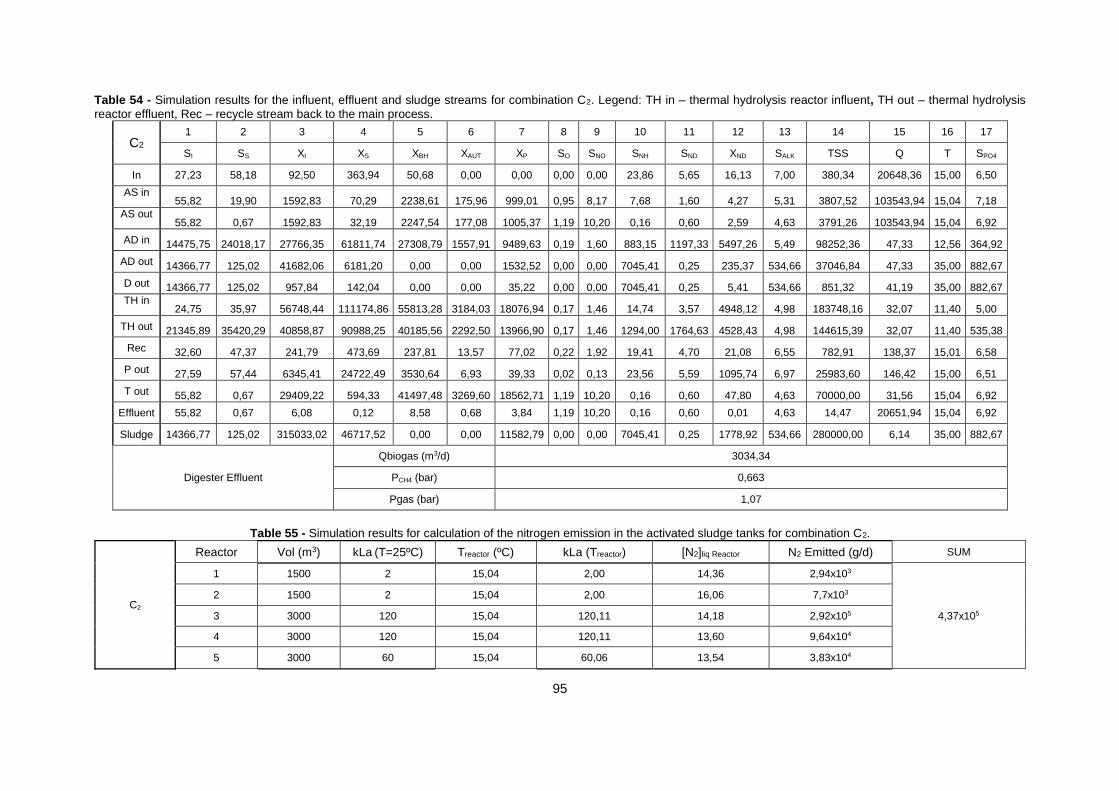
95
Table 54 - Simulation results for the influent, effluent and sludge streams for combination C2. Legend: TH in – thermal hydrolysis reactor influent, TH out – thermal hydrolysis
reactor effluent, Rec – recycle stream back to the main process.
C2 1 2 3 4 5 6 7 8 9 10 11 12 13 14 15 16 17
SI SS XI XS XBH XAUT XP SO SNO SNH SND XND SALK TSS Q T SPO4
In 27,23 58,18 92,50 363,94 50,68 0,00 0,00 0,00 0,00 23,86 5,65 16,13 7,00 380,34 20648,36 15,00 6,50
AS in 55,82 19,90 1592,83 70,29 2238,61 175,96 999,01 0,95 8,17 7,68 1,60 4,27 5,31 3807,52 103543,94 15,04 7,18
AS out 55,82 0,67 1592,83 32,19 2247,54 177,08 1005,37 1,19 10,20 0,16 0,60 2,59 4,63 3791,26 103543,94 15,04 6,92
AD in 14475,75 24018,17 27766,35 61811,74 27308,79 1557,91 9489,63 0,19 1,60 883,15 1197,33 5497,26 5,49 98252,36 47,33 12,56 364,92
AD out 14366,77 125,02 41682,06 6181,20 0,00 0,00 1532,52 0,00 0,00 7045,41 0,25 235,37 534,66 37046,84 47,33 35,00 882,67
D out 14366,77 125,02 957,84 142,04 0,00 0,00 35,22 0,00 0,00 7045,41 0,25 5,41 534,66 851,32 41,19 35,00 882,67
TH in 24,75 35,97 56748,44 111174,86 55813,28 3184,03 18076,94 0,17 1,46 14,74 3,57 4948,12 4,98 183748,16 32,07 11,40 5,00
TH out 21345,89 35420,29 40858,87 90988,25 40185,56 2292,50 13966,90 0,17 1,46 1294,00 1764,63 4528,43 4,98 144615,39 32,07 11,40 535,38
Rec 32,60 47,37 241,79 473,69 237,81 13,57 77,02 0,22 1,92 19,41 4,70 21,08 6,55 782,91 138,37 15,01 6,58
P out 27,59 57,44 6345,41 24722,49 3530,64 6,93 39,33 0,02 0,13 23,56 5,59 1095,74 6,97 25983,60 146,42 15,00 6,51
T out 55,82 0,67 29409,22 594,33 41497,48 3269,60 18562,71 1,19 10,20 0,16 0,60 47,80 4,63 70000,00 31,56 15,04 6,92
Effluent 55,82 0,67 6,08 0,12 8,58 0,68 3,84 1,19 10,20 0,16 0,60 0,01 4,63 14,47 20651,94 15,04 6,92
Sludge 14366,77 125,02 315033,02 46717,52 0,00 0,00 11582,79 0,00 0,00 7045,41 0,25 1778,92 534,66 280000,00 6,14 35,00 882,67
Digester Effluent
Qbiogas (m3/d) 3034,34
PCH4 (bar) 0,663
Pgas (bar) 1,07
Table 55 - Simulation results for calculation of the nitrogen emission in the activated sludge tanks for combination C2.
C2
Reactor Vol (m3) kLa (T=25ºC) Treactor (ºC) kLa (Treactor) [N2]liq Reactor N2 Emitted (g/d) SUM
1 1500 2 15,04 2,00 14,36 2,94x10³
4,37x10⁵
2 1500 2 15,04 2,00 16,06 7,7x10³
3 3000 120 15,04 120,11 14,18 2,92x10⁵
4 3000 120 15,04 120,11 13,60 9,64x10⁴
5 3000 60 15,04 60,06 13,54 3,83x10⁴

96
Table 56 - Simulation results for the influent, effluent, sludge and Phosnix technology underflow streams for combination C3. Legend: PT out – Phosnix technology underflow.
C3 1 2 3 4 5 6 7 8 9 10 11 12 13 14 15 16 17
SI SS XI XS XBH XAUT XP SO SNO SNH SND XND SALK TSS Q T SPO4
In 27,23 58,18 92,50 363,94 50,68 0,00 0,00 0,00 0,00 23,86 5,65 16,13 7,00 380,34 20648,36 15,00 6,50
AS in 28,14 20,13 1559,92 69,11 2193,58 168,88 973,20 1,06 7,95 7,48 1,60 4,20 5,19 3723,51 103533,89 15,16 5,67
AS out 28,14 0,67 1559,92 31,59 2202,55 169,98 979,49 1,32 9,94 0,16 0,60 2,54 4,53 3707,65 103533,89 15,16 5,40
AD in 27,39 47,56 10365,91 20522,24 10152,63 564,07 3250,49 0,24 1,84 19,48 4,72 913,33 6,54 33641,50 177,28 15,03 6,30
AD out 139,47 207,38 14699,87 2824,93 0,00 0,00 677,57 0,00 0,00 1643,35 0,54 109,61 111,65 13651,78 177,28 35,00 203,02
D out 139,47 207,38 308,75 59,33 0,00 0,00 14,23 0,00 0,00 1643,35 0,54 2,30 111,65 286,74 168,81 35,00 203,02
PT out 139,47 207,38 308,75 59,33 0,00 0,00 14,23 0,00 0,00 1611,41 0,54 2,30 111,65 286,74 168,81 35,00 34,51
P out 27,24 57,44 6343,84 24721,45 3528,72 6,65 38,31 0,02 0,13 23,55 5,59 1095,69 6,97 25979,22 146,42 15,00 6,49
T out 28,14 0,67 29451,14 596,42 41583,96 3209,11 18492,71 1,32 9,94 0,16 0,60 48,00 4,53 70000,00 30,86 15,16 5,40
Effluent 28,14 0,67 6,03 0,12 8,51 0,66 3,78 1,32 9,94 0,16 0,60 0,01 4,53 14,32 20641,89 15,16 5,40
Sludge 139,47 207,38 301496,48 57939,71 0,00 0,00 13897,14 0,00 0,00 1643,35 0,54 2248,14 111,65 280000,00 8,47 35,00 203,02
Phosnix Underflow PO4 (g/d) 28445,63
NH4 (g/d) 5391,40
Digester Effluent
Qbiogas (m3/d) 2897,25
PCH4 (bar) 0,666
Pgas (bar) 1,07
Table 57 - Simulation results for calculation of the nitrogen emission in the activated sludge tanks for combination C3.
C3
Reactor Vol (m3) kLa (T=25ºC) Treactor (ºC) kLa (Treactor) [N2]liq Reactor N2 Emitted (g/d) SUM
1 1500 2 15,16 2,01 14,32 2,83x10³
4,20x10⁵
2 1500 2 15,16 2,01 15,99 7,54x10³
3 3000 120 15,16 120,47 14,15 2,83x10⁵
4 3000 120 15,16 120,47 13,59 9,11x10⁴
5 3000 60 15,16 60,23 13,53 3,53x10⁴

97
Table 58 - Simulation results for the influent, effluent, sludge and chemical precipitation underflow streams for combination C4.Legend: RejDW1 – reject stream from the
dewatering unit of the Exelys technology (recycled back to the main process).
C4 1 2 3 4 5 6 7 8 9 10 11 12 13 14 15 16 17
SI SS XI XS XBH XAUT XP SO SNO SNH SND XND SALK TSS Q T SPO4
In 27,23 58,18 92,50 363,94 50,68 0,00 0,00 0,00 0,00 23,86 5,65 16,13 7,00 380,34 20648,36 15,00 6,50
AS in 56,52 19,91 1587,62 70,19 2234,28 177,06 996,87 0,94 8,31 7,76 1,60 4,26 5,30 3799,52 103543,83 15,05 7,24
AS out 56,52 0,67 1587,62 32,14 2243,22 178,19 1003,23 1,17 10,38 0,17 0,60 2,59 4,61 3783,30 103543,83 15,05 6,97
AD in 11388,82 18925,51 21885,31 48780,49 21530,19 1237,64 7475,45 0,19 1,70 698,54 943,87 2426,38 5,71 77494,21 60,09 13,08 288,47
AD out 11268,34 121,64 32670,34 5542,04 0,00 0,00 1371,30 0,00 0,00 5534,34 0,28 211,35 418,77 29687,75 60,09 35,00 697,02
D out 11268,34 121,64 729,17 123,69 0,00 0,00 30,61 0,00 0,00 5534,34 0,28 4,72 418,77 662,60 53,85 35,00 697,02
TH in 24,84 35,98 56698,98 111260,81 55778,95 3206,39 18052,41 0,17 1,48 14,74 3,57 4951,92 4,98 183748,16 32,05 11,40 5,00
TH out 21325,19 35443,50 40823,27 91047,91 40160,85 2308,60 13949,05 0,17 1,48 1292,76 1765,62 4530,97 4,98 144615,49 32,05 11,40 535,11
Rec 3405,39 69,68 387,86 368,73 166,24 9,56 62,99 0,15 1,36 1674,87 3,38 16,17 130,29 746,54 179,38 21,01 213,84
RejDW1 32,72 47,39 241,47 473,83 237,55 13,66 76,88 0,22 1,95 19,41 4,70 21,09 6,55 782,54 125,54 15,01 6,59
P out 27,60 57,44 6345,18 24722,40 3530,46 6,97 39,25 0,02 0,13 23,56 5,59 1095,73 6,97 25983,19 146,42 15,00 6,51
T out 56,52 0,67 29374,80 594,66 41504,84 3296,92 18562,11 1,17 10,38 0,17 0,60 47,84 4,61 70000,00 31,50 15,05 6,97
Effluent 56,52 0,67 6,07 0,12 8,57 0,68 3,83 1,17 10,38 0,17 0,60 0,01 4,61 14,46 20651,83 15,05 1,39
Sludge 11268,34 121,64 308130,22 52269,70 0,00 0,00 12933,41 0,00 0,00 5534,34 0,28 1993,36 418,77 280000,00 6,24 35,00 697,02
Chemical Precipitation Underflow PO4 (g/d) 115182,35
Digester Effluent
Qbiogas (m3/d) 3003,86
PCH4 (bar) 0,664
Pgas (bar) 1,07

98
Table 59 - Simulation results for calculation of the nitrogen emission in the activated sludge tanks for combination C4.
C4
Reactor Vol (m3) kLa (T=25ºC) Treactor (ºC) kLa (Treactor) [N2]liq Reactor N2 Emitted (g/d) SUM
1 1500 2 15,05 2,00 14,37 2,96x10³
4,41x10⁵
2 1500 2 15,05 2,00 16,07 7,75x10³
3 3000 120 15,05 120,15 14,19 2,94x10⁵
4 3000 120 15,05 120,15 13,61 9,74x10⁴
5 3000 60 15,05 60,07 13,55 3,88x10⁴
Table 60 - Simulation results for the influent, effluent, sludge, chemical precipitation underflow and Phosnix technology underflow streams for combination C5.
C5 1 2 3 4 5 6 7 8 9 10 11 12 13 14 15 16 17
SI SS XI XS XBH XAUT XP SO SNO SNH SND XND SALK TSS Q T SPO4
In 27,23 58,18 92,50 363,94 50,68 0,00 0,00 0,00 0,00 23,86 5,65 16,13 7,00 380,34 20648,36 15,00 6,50
AS in 28,14 20,24 1560,08 69,17 2197,45 168,86 974,96 1,05 7,89 7,48 1,60 4,20 5,19 3727,89 103533,89 15,16 5,67
AS out 28,14 0,67 1560,08 31,66 2206,44 169,96 981,27 1,31 9,86 0,16 0,60 2,55 4,53 3712,06 103533,89 15,16 5,40
AD in 27,40 47,55 10364,31 20518,25 10163,46 563,90 3255,72 0,24 1,82 19,48 4,72 913,16 6,54 33649,23 177,32 15,03 6,30
AD out 139,38 277,93 14704,18 2823,57 0,00 0,00 677,21 0,00 0,00 1644,12 0,54 109,56 111,71 13653,72 177,32 35,00 203,23
D out 139,38 277,93 308,84 59,31 0,00 0,00 14,22 0,00 0,00 1644,12 0,54 2,30 111,71 286,78 168,84 35,00 203,23
PT out 139,38 277,93 308,84 59,31 0,00 0,00 14,22 0,00 0,00 1612,15 0,54 2,30 111,71 286,78 168,84 35,00 34,55
P out 27,24 57,44 6343,86 24721,51 3528,88 6,65 38,38 0,02 0,13 23,55 5,59 1095,69 6,97 25979,45 146,42 15,00 6,49
T out 28,14 0,67 29419,14 597,01 41607,92 3205,01 18504,25 1,31 9,86 0,16 0,60 48,05 4,53 70000,00 30,89 15,16 5,40
Effluent 28,14 0,67 6,02 0,12 8,52 0,66 3,79 1,31 9,86 0,16 0,60 0,01 4,53 14,33 20641,89 15,16 1,08
Sludge 139,38 277,93 301541,97 57903,59 0,00 0,00 13887,77 0,00 0,00 1644,12 0,54 2246,84 111,71 280000,00 8,47 35,00 203,23
Chemical Precipitation Underflow PO4 (g/d) 89200,05
Phosnix Underflow PO4 (g/d) 28480,63
NH4 (g/d) 5398,03
Digester Effluent
Qbiogas (m3/d) 2893,33
PCH4 (bar) 0,665
Pgas (bar) 1,07

99
Table 61 - Simulation results for calculation of the nitrogen emission in the activated sludge tanks for combination C5.
C5
Reactor Vol (m3) kLa (T=25ºC) Treactor (ºC) kLa (Treactor) [N2]liq Reactor N2 Emitted (g/d) SUM
1 1500 2 15,16 2,01 14,33 2,87x10³
4,21x10⁵
2 1500 2 15,16 2,01 16,00 7,57x10³
3 3000 120 15,16 120,47 14,16 2,84x10⁵
4 3000 120 15,16 120,47 13,59 9,14x10⁴
5 3000 60 15,16 60,23 13,53 3,55x10⁴
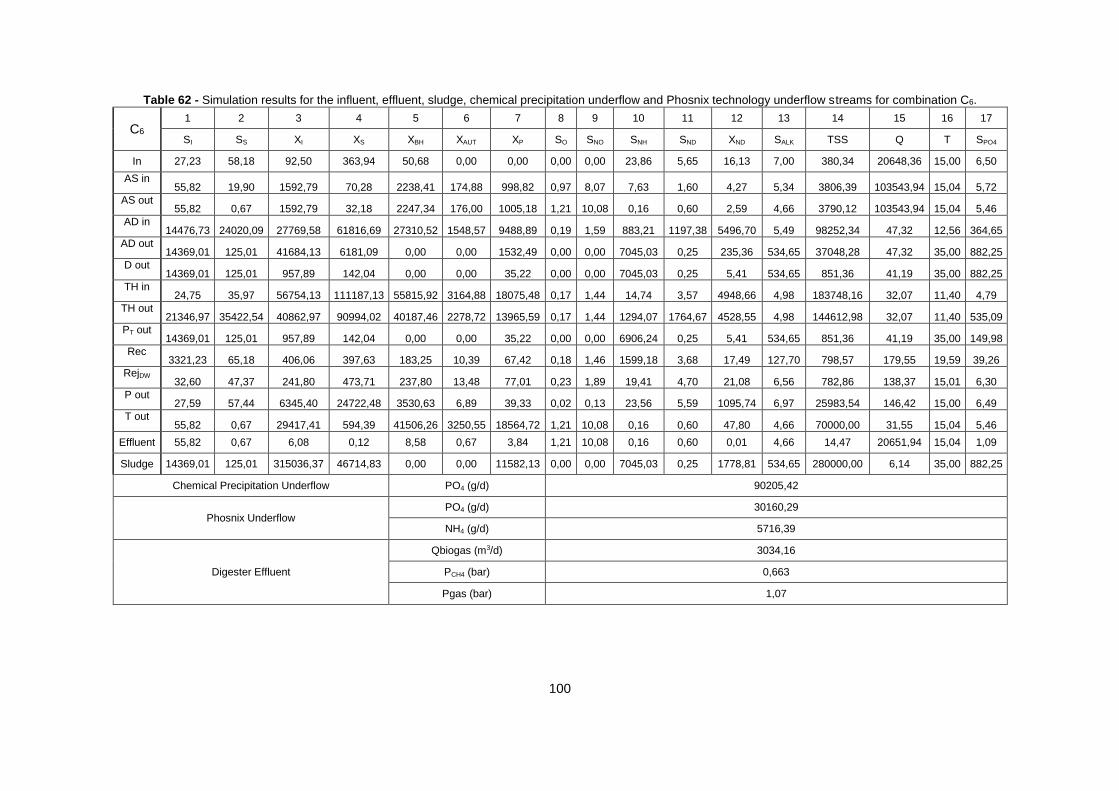
100
Table 62 - Simulation results for the influent, effluent, sludge, chemical precipitation underflow and Phosnix technology underflow streams for combination C6.
C6 1 2 3 4 5 6 7 8 9 10 11 12 13 14 15 16 17
SI SS XI XS XBH XAUT XP SO SNO SNH SND XND SALK TSS Q T SPO4
In 27,23 58,18 92,50 363,94 50,68 0,00 0,00 0,00 0,00 23,86 5,65 16,13 7,00 380,34 20648,36 15,00 6,50
AS in 55,82 19,90 1592,79 70,28 2238,41 174,88 998,82 0,97 8,07 7,63 1,60 4,27 5,34 3806,39 103543,94 15,04 5,72
AS out 55,82 0,67 1592,79 32,18 2247,34 176,00 1005,18 1,21 10,08 0,16 0,60 2,59 4,66 3790,12 103543,94 15,04 5,46
AD in 14476,73 24020,09 27769,58 61816,69 27310,52 1548,57 9488,89 0,19 1,59 883,21 1197,38 5496,70 5,49 98252,34 47,32 12,56 364,65
AD out 14369,01 125,01 41684,13 6181,09 0,00 0,00 1532,49 0,00 0,00 7045,03 0,25 235,36 534,65 37048,28 47,32 35,00 882,25
D out 14369,01 125,01 957,89 142,04 0,00 0,00 35,22 0,00 0,00 7045,03 0,25 5,41 534,65 851,36 41,19 35,00 882,25
TH in 24,75 35,97 56754,13 111187,13 55815,92 3164,88 18075,48 0,17 1,44 14,74 3,57 4948,66 4,98 183748,16 32,07 11,40 4,79
TH out 21346,97 35422,54 40862,97 90994,02 40187,46 2278,72 13965,59 0,17 1,44 1294,07 1764,67 4528,55 4,98 144612,98 32,07 11,40 535,09
PT out 14369,01 125,01 957,89 142,04 0,00 0,00 35,22 0,00 0,00 6906,24 0,25 5,41 534,65 851,36 41,19 35,00 149,98
Rec 3321,23 65,18 406,06 397,63 183,25 10,39 67,42 0,18 1,46 1599,18 3,68 17,49 127,70 798,57 179,55 19,59 39,26
RejDW 32,60 47,37 241,80 473,71 237,80 13,48 77,01 0,23 1,89 19,41 4,70 21,08 6,56 782,86 138,37 15,01 6,30
P out 27,59 57,44 6345,40 24722,48 3530,63 6,89 39,33 0,02 0,13 23,56 5,59 1095,74 6,97 25983,54 146,42 15,00 6,49
T out 55,82 0,67 29417,41 594,39 41506,26 3250,55 18564,72 1,21 10,08 0,16 0,60 47,80 4,66 70000,00 31,55 15,04 5,46
Effluent 55,82 0,67 6,08 0,12 8,58 0,67 3,84 1,21 10,08 0,16 0,60 0,01 4,66 14,47 20651,94 15,04 1,09
Sludge 14369,01 125,01 315036,37 46714,83 0,00 0,00 11582,13 0,00 0,00 7045,03 0,25 1778,81 534,65 280000,00 6,14 35,00 882,25
Chemical Precipitation Underflow PO4 (g/d) 90205,42
Phosnix Underflow PO4 (g/d) 30160,29
NH4 (g/d) 5716,39
Digester Effluent
Qbiogas (m3/d) 3034,16
PCH4 (bar) 0,663
Pgas (bar) 1,07

101
Table 63 - Simulation results for calculation of the nitrogen emission in the activated sludge tanks for combination C6.
C6
Reactor Vol (m3) kLa (T=25ºC) Treactor (ºC) kLa (Treactor) [N2]liq Reactor N2 Emitted (g/d) SUM
1 1500 2 15,04 2,00 14,35 2,91x10³
4,34x10⁵
2 1500 2 15,04 2,00 16,04 7,66x10³
3 3000 120 15,04 120,11 14,18 2,90x10⁵
4 3000 120 15,04 120,11 13,60 9,54x10⁴
5 3000 60 15,04 60,06 13,54 3,78x10⁴
Table 64 - Simulation results for the influent, effluent, sludge and Phosnix technology underflow streams for combination C7.
C7 1 2 3 4 5 6 7 8 9 10 11 12 13 14 15 16 17
SI SS XI XS XBH XAUT XP SO SNO SNH SND XND SALK TSS Q T SPO4
In 27,23 58,18 92,50 363,94 50,68 0,00 0,00 0,00 0,00 23,86 5,65 16,13 7,00 380,34 20648,36 15,00 6,50
AS in 38,22 19,91 1592,29 70,28 2238,45 175,71 998,54 0,96 8,15 7,67 1,60 4,27 5,33 3806,44 103544,15 15,04 5,73
AS out 38,22 0,67 1592,29 32,18 2247,37 176,83 1004,90 1,20 10,18 0,16 0,60 2,59 4,65 3790,18 103544,15 15,04 5,46
AD in 4670,75 7742,66 27780,60 61776,66 27326,06 1556,74 9491,90 0,19 1,60 883,54 1198,12 5500,57 5,49 98252,04 47,30 12,56 364,88
AD out 5519,23 141,36 41356,68 5158,29 0,00 0,00 1273,83 0,00 0,00 7124,46 0,25 196,93 540,33 35841,60 47,30 35,00 888,96
D out 5519,23 141,36 945,78 117,96 0,00 0,00 29,13 0,00 0,00 7124,46 0,25 4,50 540,33 819,65 41,36 35,00 888,96
TH in 22,24 35,97 56744,76 111186,27 55816,31 3179,81 18070,39 0,17 1,45 14,74 3,57 4948,63 4,98 183748,16 32,07 11,40 4,79
TH out 6874,54 11396,44 40856,23 90883,72 40187,75 2289,46 13962,17 0,17 1,45 1293,83 1764,76 4528,77 4,98 144531,07 32,07 11,40 535,13
PT out 5519,23 141,36 945,78 117,96 0,00 0,00 29,13 0,00 0,00 6984,62 0,25 4,50 540,33 819,65 41,36 35,00 151,12
Rec 1292,60 69,00 403,76 391,85 183,08 10,43 65,98 0,17 1,47 1622,19 3,68 17,27 129,39 791,33 179,76 19,61 39,63
Rej DW 29,29 47,37 241,76 473,71 237,81 13,55 76,99 0,22 1,91 19,41 4,70 21,08 6,56 782,86 138,39 15,01 6,31
P out 27,37 57,44 6345,38 24722,48 3530,64 6,92 39,31 0,02 0,13 23,56 5,59 1095,74 6,97 25983,55 146,42 15,00 6,49
T out 38,22 0,67 29407,62 594,41 41506,23 3265,83 18559,24 1,20 10,18 0,16 0,60 47,81 4,65 70000,00 31,55 15,04 5,46
Effluent 38,22 0,67 6,08 0,12 8,58 0,68 3,84 1,20 10,18 0,16 0,60 0,01 4,65 14,47 20652,15 15,04 5,46
Sludge 5519,23 141,36 323084,66 40297,36 0,00 0,00 9951,32 0,00 0,00 7124,46 0,25 1538,43 540,33 280000,00 5,93 35,00 888,96
Phosnix Underflow PO4 (g/d) 30520,03
NH4 (g/d) 5784,57
Digester Effluent
Qbiogas (m3/d) 2471,71
PCH4 (bar) 0,680
Pgas (bar) 1,06

102
Table 65 - Simulation results for calculation of the nitrogen emission in the activated sludge tanks for combination C7.
C7
Reactor Vol (m3) kLa (T=25ºC) Treactor (ºC) kLa (Treactor) [N2]liq Reactor N2 Emitted (g/d) SUM
1 1500 2 15,04 2,00 14,36 2,93x10³
4,37x10⁵
2 1500 2 15,04 2,00 16,05 7,69x10³
3 3000 120 15,04 120,11 14,18 2,92x10⁵
4 3000 120 15,04 120,11 13,60 9,61x10⁴
5 3000 60 15,04 60,06 13,54 3,82x10⁴
Table 66 – Liquid oxygen concentrations in the different activated sludge tanks (g/m3). Valid for every combination, referred in Section 3.4.2.1.
Reactor 1 Reactor 2 Reactor 3 Reactor 4 Reactor 5
[O2]liq (g/m3) 0,0093 1,0970 x10⁻⁴ 0,4663 1,4284 1,3748
Table 67 – Simulation flow rates for calculation of the pumping energy costs for the different configurations (m3/d), referred in Section. 3.4.2.1.
Combination Qint Qr Qw Qpu Qtu Qdo Qth
C0 61944 20648 300 146,42 30,87 168,82 ---
C1 61944 20648 300 146,42 30,90 168,85 ---
C2 61944 20648 300 146,42 31,56 41,19 32,07
C3 61944 20648 300 146,42 30,86 168,81 ---
C4 61944 20648 300 146,42 31,50 53,85 32,05
C5 61944 20648 300 146,42 30,89 168,84 ---
C6 61944 20648 300 146,42 31,55 41,19 32,07
C7 61944 20648 300 146,42 31,55 41,36 32,07

103