techniques load cells used at the full -scale complex · of the pseudo load cell. pseudo load...
TRANSCRIPT

NASA Technical Memorandum 86693
Experimental Techniques for Three-Axes Load Cells Used at the National Full -Scale Aerodynamics Complex Michael R. Dudley
(USA-28-86693) EXPERIBENTAL TECBUXQUSS FOR M07-20544
168EE-AXES LOAD CELLS KSEO AI IEE IAZLTIOIAL FULL-SCALE I E G O D Y IlABICS COBFLEX (HASA) 55 Unclas F A v a i l : NTIS BC AOU/tlP A01 CSCL O l C
G3/05 0057834
September 1985
National Aeronautics and Space Administration
I ... r.....
Date for general release Seg”rember 198’7 I
https://ntrs.nasa.gov/search.jsp?R=19870019113 2019-05-06T16:41:41+00:00Z

NASA Technical Memorandum 86693
Experimental Techniques for Three-Axes Load Cells Used at the National Full =Scale Aerodynamics Complex
~
Michael R. Dudley, Ames Research Center, Moffett Field, California
September 1985
National Aeronautics and Space Ad mi n 1st ration
Ames Research Center Moffett Field, California 94035

SUMMARY
This memorandum provides the necessary information for an aerodynamic investi- gation requiring load cell force measurements at the National Full-scale Aerody- namics Complex (NFAC). Included here are details of the Ames 40 by 80 three- component load cells; typical model/load cell installation geometries; transducer signai conditioning; a description of tiia hies Staiidard Crmputations Wind T u m z l Data Reduction Program for Load Cells Forces and Moments (SCELLS), and the inputs required for SCELLS. The Outdoor Aerodynamic Facilities Complex (OARF), a facility within the NFAC where three-axes load cells serve as the primary balance system, is used as an example for many of the techniques, but the information applies equally well to other static and wind tunnel facilities that make use of load cell balances.
This paper can serve either as a user guide for NASA and contract engineers who are preparing to conduct an investigation at the OARF or at the NFAC, or as a description of techniques, data systems, and hardware that is currently used for ground-based aerodynamic investigations which measure forces with three-axes load cells.
INTRODUCTION
Ground-based aerodynamic investigations of full-scale models require a means of measuring the forces that are generated by the model. Aerodynamics Complex (NFAC), strain gage transducer load cells, internal balances, and external balances are used for this purpose. For test conditions where the model weight exceeds the capacity of the internal balances (1250 kg), and where the external balances dedicated to the full-scale wind tunnels cannot be utilized, combinations of load cells are used to form a balance system (for example, outdoor testing or when measuring isolated forces on model components. The two types of load cells used at the NFAC are single axis and three component. The three compo- nent load cells (three-AX LC) are designed to measure forces in three orthogonal directions. in only one direction.
At the National Full-scale
The single-axis load-cells (one-Ax LC) are capable of force measuremept
LOAD CELLS
The Ames 40 by 80 three-component load cells were designed at Ames specifically for large-model testing at the NFAC. The general arrangement of a three-Ax LC is a
1

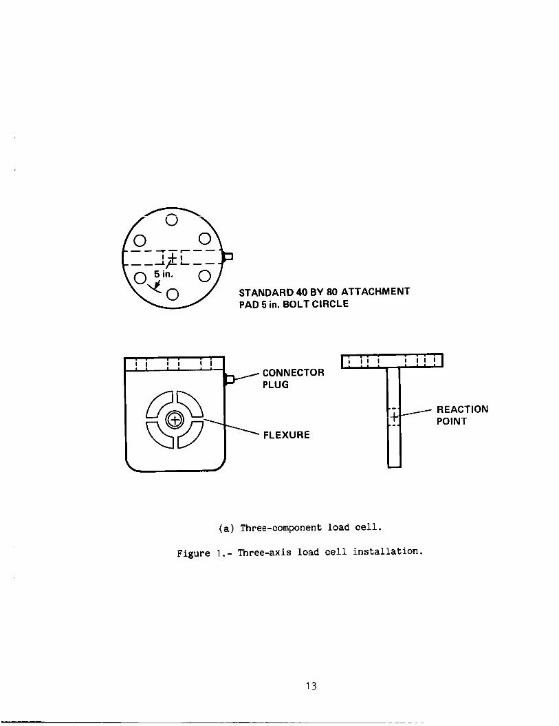
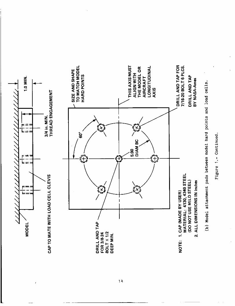
pin bushing suspended in a flat plate by load flexures. perpendicular to a mounting pad. 5-in. bolt circle, figure 1. The flexures are instrumented with resistance-type, four-arm strain gage bridges. system of bridges) is designed to measure force in one of the three orthogonal directions. Hereafter each bridge network will be referred to as a gage of the load cell; i.e., the bridge circuit measuring axial force on three-Ax LC number one would be the axial gage of load cell number one.
The flat plate is attached The pad is drilled with the standard 40 by 80
Each bridge (or in the case of redundant bridges,
A single-axis load cell consists of a single flexure instrumented with a four- arm strain gage network. It is only capable of unidirectional force measurements and will be damaged if loaded perpendicular to its axis. On occasion three, one-Ax LC are used in combination so that all three axes intersect a single point in space. This is done to form a single, three-component pseudoload cell. When this is done, each one-Ax LC is referred to as a gage or component of the pseudoload cell. These pseudoload cells are a convenient convention that simplifies the Ames Standard Computations Wind Tunnel Data Reduction Program for Load Cells Forces and Moments (SCELLS) used at the NFAC.
All load cells used in experimental investigations at Ames are calibrated at the Ames Reliability and Quality Assurance laboratory (RQ&A). resistance calibrations and loadings to determine the repeatability and linearity of the voltage to force ratios (primary conversions constants). interactions (the apparent change of a gage force when a perpendicular force is applied) are also determined. inaccuracies of less than 0.1% for the one-Ax LC and 0.3% for the three-Ax LC. Installed system inaccuracies are usually about 1% of the full-scale range of the gage. An example of a typical load cell calibration for one gage of a three-Ax LC by RQ&A is included in appendix A.
The work includes
For the three-Ax LC,
The primary voltage/force conversions generally have
Although calibrations of the side force gages of the three-Ax LC are usually good in the laboratory, historically it has been difficult to measure the side force on a model at the Outdoor Aerodynamics Facility Complex (OARF), a facility within the NFAC. This is thought to be a result of the installation methods which are discussed in the following sections.
INSTALLATION
Conventional Model Installations
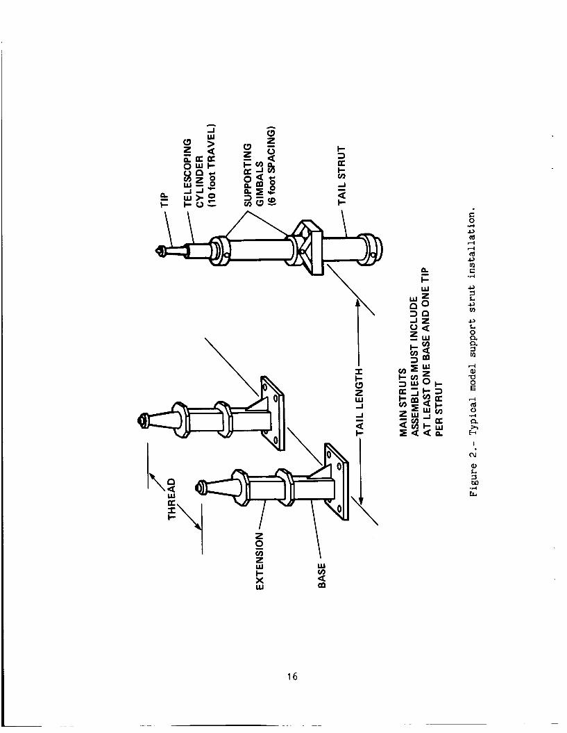
Normally, models are mounted at the NFAC on a support system which consists of two main struts and a tail strut. The model height and pitch angle are varied using different combinations of strut tips or extensions, and a continuously telescoping tail strut. It is possible to vary the tread of the main struts and their distance from the tail strut. Discrete model installation heights are between 0.5 m and 6.5 m, at the OARF, and at the 40- by 80-Foot Wind tunnel, and are up to 15 m in the 80 by 120 test section. An
The tail strut is supported at its base by a gimbal.
2
L
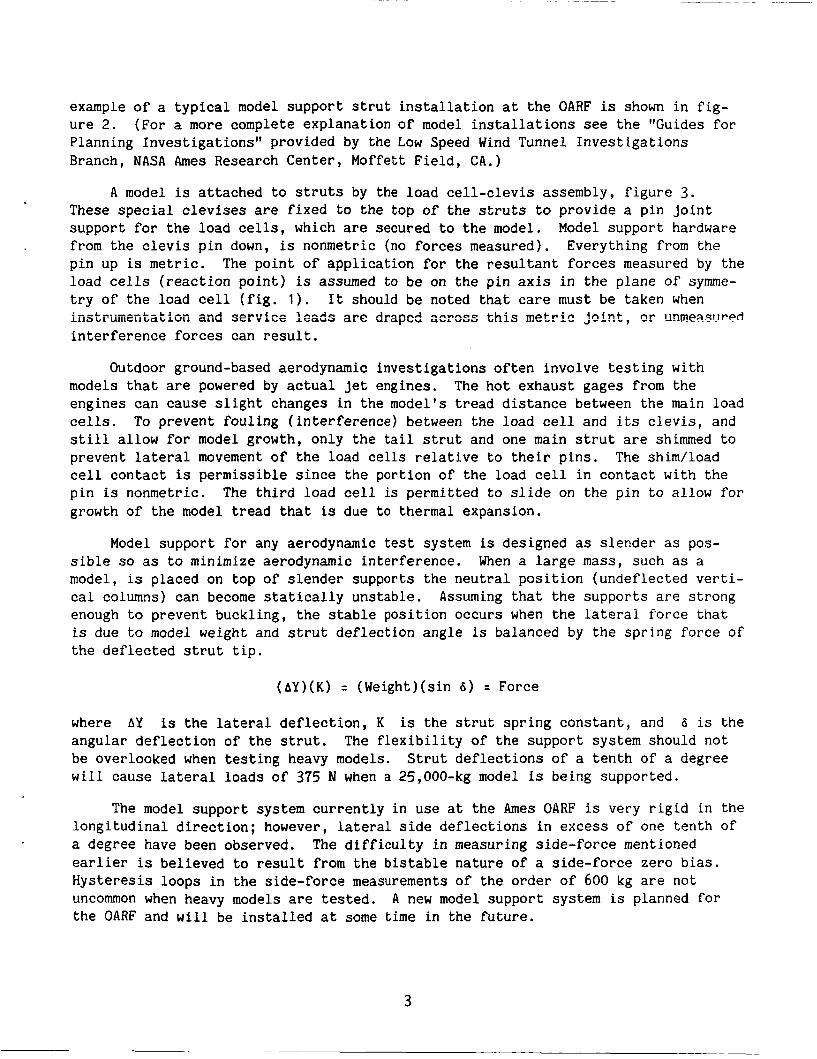
example of a t y p i c a l model s u p p o r t s t r u t i n s t a l l a t i o n a t the OARF is shown i n f i g - u r e 2. Planning I n v e s t i g a t i o n s ” provided by t h e Low Speed Wind Tunnel I n v e s t i g a t i o n s Branch, NASA Ames Research C e n t e r , Moffett F i e l d , CA. )
(For a more complete exp lana t ion of model i n s t a l l a t i o n s see t h e “Guides f o r
A model is a t t a c h e d t o s t r u t s by the l o a d c e l l - c l e v i s assembly, f i g u r e 3 . These s p e c i a l c l e v i s e s are f i x e d to t h e top of t h e s t r u t s t o p r o v i d e a p i n j o i n t s u p p o r t for t h e l o a d cel ls , which are secured t o t h e model. Model s u p p o r t hardware from the c l e v i s p i n down, is nonmetric (no f o r c e s measured). Every th ing from t h e p i n up is metric. The p o i n t of a p p l i c a t i o n f o r t h e r e s u l t a n t forces measured by t h e load cel ls (reaction p o i n t ) is assumed t o b e on t h e p i n a x i s i n t h e p l ane of symme- t r y of t h e load cell ( f i g . 1 ) . iiistr-uiientation sild service leads sr2 draped aC!r=ss t h i s metric jn int , i n t e r f e r e n c e forces can r e s u l t .
I t should be noted t h a t care must be taken when nr unmPasr_lrPc!
Outdoor ground-based aerodynamic i n v e s t i g a t i o n s o f t e n invo lve t e s t i n g wi th models t h a t are powered by a c t u a l j e t engines . The h o t exhaus t gages from t h e eng ines can cause s l i g h t changes i n t h e model’s tread d i s t a n c e between t h e main load cells. To p reven t f o u l i n g ( i n t e r f e r e n c e ) between t h e load cel l and its c lev is , and s t i l l a l low f o r model growth, o n l y the t a i l s t r u t and one main s t r u t are shimmed t o p reven t la teral movement of t h e load cells r e l a t i v e to t h e i r p i n s . c e l l c o n t a c t is p e r m i s s i b l e s i n c e t h e po r t ion o f t h e load ce l l i n c o n t a c t w i th t h e p i n is nonmetric. The t h i r d load cell is pe rmi t t ed to s l i d e on t h e p i n t o a l low f o r growth o f t h e model tread t h a t is due t o thermal expansion.
The shim/load
Model suppor t f o r any aerodynamic t es t system is des igned as s l e n d e r as pos- s i b l e so as t o minimize aerodynamic i n t e r f e r e n c e . When a l a r g e mass, such as a model, is placed on t o p o f s l e n d e r suppor t s t h e n e u t r a l p o s i t i o n ( u n d e f l e c t e d v e r t i - cal columns) can become s t a t i c a l l y uns t ab le . enough to p reven t buck l ing , t h e s tab le p o s i t i o n o c c u r s when t h e la teral f o r c e t n a t is due to model weight and s t r u t d e f l e c t i o n a n g l e is balanced by t h e s p r i n g f o r c e of t he deflected s t r u t t i p .
Assuming t h a t t he s u p p o r t s are s t r o n g
(AY)(K) = (Weight ) ( s in 6 ) = Force
where AY is t h e lateral d e f l e c t i o n , K is t h e s t r u t s p r i n g c o n s t a n t , and 6 is t h e angu la r d e f l e c t i o n of t h e s t r u t . be overlooked when t e s t i n g heavy models. w i l l cause la teral l o a d s of 375 N when a 25,000-kg model is being suppor t ed .
The f l e x i b i l i t y of t h e s u p p o r t system should n o t S t r u t d e f l e c t i o n s o f a t e n t h o f a degree
The model s u p p o r t system c u r r e n t l y i n use a t t h e Ames OARF is very r i g i d i n t he l o n g i t u d i n a l d i r e c t i o n ; however, lateral side d e f l e c t i o n s i n e x c e s s o f one t e n t h of a degree have been observed. The d i f f i c u l t y i n measuring side-force mentioned earlier is b e l i e v e d to r e s u l t from t h e b i s t ab le n a t u r e o f a s i d e - f o r c e z e r o bias. H y s t e r e s i s l oops i n t h e side-force measurements o f t he o r d e r o f 600 kg are no t uncommon when heavy models are tested. A new model s u p p o r t system is planned f o r t h e OARF and w i l l be i n s t a l l e d a t some time i n t h e f u t u r e .
3

Jet-Propulsion Test stand Installation
The NFAC Jet-Propulsion test stand was developed to accommodate the testing of engine components such as nozzles and inlets and small models that can be conve- niently attached to a platform. The test stand consists of a metric table suspended by links from a nonmetric support platform. links contain single-axis load cells that determine the forces which are transmitted by the links. vertical links. The motion of the table is confined in the horizontal plane by two axial and two side links. used for a nonredundant system. intersect at no more than four points in space. achieved by various coplanar link orientations.
All the supporting and restraining
The links are arranged so that the metric table is hung by four
Typically only three of the four horizontal links are The axes of all the links are positioned so they
Figure 4 illustrates how this is
The four points define the location of four pseudo load cells. The individual gage forces are measured by the one-Ax LC that corresponds to the appropriate axis of the pseudo load cell. pseudo load cells, remember that the one-Ax LC can only be assigned once. ple, if the forward side link is to be defined as side-force for load cell one (the load cell at the forward left), there would be no side-force gage for load cell two (forward right).
When assigning single-axis load cells as components of For exam-
When installing the load-links in the Jet-Propulsion test stand, care must be taken not t o induce any adverse preloads while tightening the links. description of the link installations, see appendix B.
For a detailed
Load Cell Number Assignments
In the data reduction program SCELLS reference to a particular load cell gage is made via the subscripts (m,n) (see table 1 ) . The subscript "m" denotes the component direction; 1 = X (axial), 2 = Y (side), and 3 = 2 (normal). The "n" subscript indicates the load cell number and has a maximum value of four.
Although any numbering assignments that are used consistently throughout a test are acceptable, it is recommended that the conventions above be followed whenever possible to avoid confusion when dealing with the instrumentation and programming groups.
LOAD CELL POSITION AND ORIENTATION
Reaction Point Moment Arm
The position of each load cell or pseudo load cell is defined in a Cartesian
(The moment center can be any coordinates system which is parallel to the model's body axes. system is located at the moment center of the model. arbitrary point in space but usually has some physical significance, such as the
The origin of this
4

p r e d i c t e d c e n t e r of g r a v i t y of the aircraft be ing modeled.) f o r these c o o r d i n a t e s are d e f i n e d as:
The p o s i t i v e d i r e c t i o n s
P o s i t i v e X , i n t h e p o s i t i v e d r a g d i r e c t i o n , axial t o t he rear, p a r a l l e l t o t h e axis of t h e model.
P o s i t i v e Y , i n t h e p o s i t i v e side f o r c e d i r e c t i o n , t o t h e r i g h t , pe rpend icu la r t o t h e model ' s plane-of-symmetry.
P o s i t i v e Z , i n t he p o s i t i v e l i f t d i r e c t i o n , up, normal to t h e X- and Y-axes.
A l oad c e l l p laced t o t h e rear, r i g h t , and above t h e moment c e n t e r would have a l l p o s i t i v e c o o r d i n a t e s .
When it is necessa ry to d e f i n e t h e load ce l l as a p o i n t i n s p a c e , such as f o r de t e rmin ing d i s t a n c e s t o t h e moment c e n t e r , t h e r e a c t i o n p o i n t d i s c u s s e d above, f i g u r e 1 , should be used as t h a t p o i n t .
The c o o r d i n a t e s of each load c e l l a r e i n p u t t o SCELLS as t h e c o n s t a n t s XYZLCM (m,n). In t h i s case, "m" i n d i c a t e s t h e d i r e c t i o n o f t h e measurement (e i ther 1 , 2 , o r 3 as d e f i n e d above for axes d i r e c t i o n s ) and "n" t h e load ce l l number. The XYZLCM v a l u e s are used i n t h e computation of t h e r e s u l t a n t moments as seen by t h e model so t h e l i n e a l dimension i n t h e moments w i l l be t h e same u n i t s as t h e distances i n p u t , i .e . , i f f o r c e is be ing measured i n pounds, i n p u t t i n g XYZLCM i n f e e t w i l l r e s u l t i n moments c a l c u l a t e d i n foot-pounds.
Angular O r i e n t a t i o n
When load cel ls are mounted on a model, t h e r e are o f t e n a n g u l a r misalignments between t h e axes of t he load cells and t h e model. T h i s can occur either from s l i g h t e r r o r s i n t h e f a b r i c a t i o n o f t he mounting pads o r i n t h e i n t e n t i o n a l r o t a t i o n s t h a t are due to some s p e c i a l i n s t a l l a t i o n requirements. All these a n g l e s must be accounted f o r d u r i n g data r e d u c t i o n i n o rde r t o avoid c o s i n e e r r o r s when r e so lv ing t.hp forces. a n g l e s t h a t each model axis must be r o t a t e d t o i n o r d e r t o a l i g n each one with t h e f o r c e measuring axis o f each l o a d ce l l .
Tn annomplish t h i s , i npu t s must be made t o SCELLS t h a t d e f i n e the
G e n e r a l l y , it is on ly necessa ry t o make r o t a t i o n s abou t one or two axes; how- e v e r , should it be r e q u i r e d t o rotate t h e axes through t h r e e a n g l e s t h e order of r o t a t i o n and how t h e a n g l e s are referenced become impor tan t . two a n g l e s o r less o r f o r a n g l e s o f less than f i v e deg rees , t h e program i n p u t s f o r load cel l 'In" are:
For t h e s imple case of
XLCPSI(n), yaw a n g l e of load ce l l "ntl; Ro ta t ion abou t t h e Z a x i s , p o s i t i v e a n g l e s occur when t h e forward edge of t h e load-cell is t o the l e f t of a l i n e p a r a l l e l t o t h e model p l ane o f symmetry.
5

XLCTHE(n), pitch angle of load cell 'In"; Rotation about the Y axis, positive angles occur when the forward edge of the mounting pad is higher than the rear edge.
XLCPHE(n), roll angle of load cell "n"; Rotation about the X axis, positive angles occur when the right edge of the mounting pad is higher than the left edge.
The angles are illustrated in figure 5. All angles are measured in degrees.
For the more complicated case of three rotations of significant magnitude, the following rules apply: XLCPSI(n), XLCTHE(n), XLCPHE(n); the angles are each equal to a rotation for the model's body axes that brings a specific axis coincident with a particular load cell's axis; for each load cell the model axes are rotated in the sequence mentioned above. In detail:
The angles must be determined in the eulerian order,
XLCPSI(n), the model's axes are rotated about their Z-axis until the model's Y-axis is in the Y-Z plane of the load cell.
XLCTHE(n), the intermediate axes are rotated about their X-axis is coincident with the load cell's X-axis.
Y-axis until the
XLCPHE(n1, the second intermediate axes system is rotated about its until all the axes are coincident with the load cell's axes system.
X-axis
The positive sense of the angles are defined according to the right-hand rule which states: Clockwise rotations are positive when the viewer is facing in the positive direction of the axis of rotation. axes of rotation is the same as described above for the reaction point moment arm; +X is rearward, +Y is to the right, and +Z is in an upward position.
In this case the positive sense of the
CONVERSION CONSTANTS (data reduction)
The load cell is a transducer that produces an electrical signal whose voltage is proportional to the force experienced by the cell. The signal conditioning and data acquisition networks amplify the signal, convert it to digital counts propor- tional to the voltage, and record a time-averaged value of the counts in the com- puter storage area. reflect the actual loads measured, it is necessary to multiply the counts by a conversion constant, conditioning methods and define the conversion constants used by the data reduction program SCELLS. provided.
To translate the recorded value into engineering units that
The following paragraphs give a brief summary of the signal
An explanation of how the constants are obtained by the engineer is
6

SIGNAL CONDITIONING
The change in a load cell's signal output is proportional to the change in the force which is applied to the load cell and the excitation voltage which is applied to the bridge network. being converted to digital counts. After the signal is in a digital form, addi- tional gains can be made by the signal conditioning cards. The digital gains are often referred to as programmable gains by virtue of their ability to be set by a computer operator during initialization. with any gains or conversions which are written into data reduction programs.
This signal can be increased by a voltage amplifier before
Programmable gains should not be confused
As t.he systems i.ised at the NFAC are presently configured, voltage amplification is made with Newport or Pacific amplifiers. Typical gain adjustments on these amps are 1 , 2, 5, 10, 20, 50, 100, 200, 500, 1000. Any multiplexed signals are condi- tioned by RMDU (remote multiplexing-demultiplexing unit) cards. The PSF (preampli- fying sample filtering) cards have set hardware gains with 128 being the most common one. The AMX (analog to digital multiplexing) and DMX (digital multiplexing) cards are also used for signal conditioning. computer are multiplexed and go through the RCU (RMDU control unit). fixed conversion ratios of 3200 or 3333 counts per volt for any multiplexed analog signal. gains. the values of 1 , 2, 4, 16, 64, 128, 256, 512. (Binary except for 8 and 32.)
All signals that will be passed to the The RMDUs have
This acts as an additional gain independent of the voltage or programmable The binary programmable gains are set by the computer operator and can have
PRIMARY CONVERSION CONSTANTS, CLDCLS(s, m, n); [force/counts]
The CLDCLS constants are a product of the primary laboratory calibration and the signal gains between the load cell and the computer. The laboratory calibration provides the force to voltage relation for the load cell, and the voltage to counts change is determined by the product of the gains. trates how t o calculate CLDCLS
The following equation illus-
Primary conv. (Amp gain)(A/D conv.)(Programmable gain) CLDCLS(s,m,n) =
In dimensional form:
[force/voltl [force/count 1 = [ volt/vol t 1 [ count/volt 1 count/count 1
(See appendix C for a sample numerical calculation of CLDCLS.)
The "m" and W' subscripts indicate load cell component and number as explained above. positive or negative loading (sometimes referred to as the bidirectional loading subscript). loading. tains the computed primary slopes loaded in two directions, for each gage. determining the CLDCLS constants, the user should verify that the lab definition of positive loading for each gage is consistent with the definitions of the data reduc- tion program for positive loads as described above. necessary to exchange the lrs" subscripts for the CLDCLS constants for the incon- sistent gages.
The '*s" subscript indicates whether the conversion constant applies for
A subscript of "1" implies positive loading, "2" implies negative The load cell calibration provided by the RQ&A lab (see appendix A) con-
When
If they are not, it may be
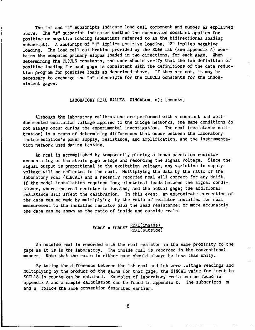
LABORATORY RCAL VALUES, XINCAL(m, n); [counts]
Although the laboratory calibrations are performed with a constant and well- documented excitation voltage applied to the bridge networks, the same conditions do not always occur during the experimental investigation. The rcal (resistance Cali- bration) is a means of determining differences that occur between the laboratory instrumentation's power supply, resistance, and amplification, and the instrumenta- tion network used during testing.
An rcal is accomplished by temporarily placing a known precision resistor across a leg of the strain gage bridge and recording the signal voltage. signal output is proportional to the excitation voltage, any variation in supply voltage will be reflected in the rcal. Multiplying the data by the ratio of the laboratory rcal (XINCAL) and a recently recorded rcal will correct for any drift. If the model installation requires long electrical leads between the signal condi- tioner, where the rcal resistor is located, and the actual gage; the additional resistance will affect the calibration. the data can be made by multiplying measurement to the installed resistor plus the lead resistance; or more accurately the data can be shown as the ratio of inside and outside rcals.
Since the
In this event, an approximate correction of by the ratio of resistor installed for rcal
RCAL( inside ) FGAGE = FCAGE* RCAL(outside1
An outside rcal is recorded with the rcal resistor in the same proximity to the gage as it is in the laboratory. manner.
The inside rcal is recorded in the conventional Note that the ratio in either case should always be less than unity.
By taking the difference between the lab rcal and lab zero voltage readings and multiplying by the product of the gains for that gage, the XINCAL value for input to SCELLS in counts can be obtained. appendix A and a sample calculation can be found in appendix C. and n follow the same convention described earlier.
Examples of laboratory rcals can be found in The subscripts m
8

INTERACTIONS CONSTANTS
DADS( s , n ) , DADN( s , n 1, DSDA ( s ,n , DSDN( s , n , DNDA( s , n , DNDS( s , n
The body of a three-component load cell is fabricated from a single piece of material. When a force is applied in a given direction, unavoidably, the gages perpendicular to the load also experience some deflection. These unwanted deflec- tions result in "apparent" forces being indicated normal to an applied load. The computed gage forces can be corrected for interactions by multiplying the influence coefficient (interaction constant) times load to determine the magnitude of the apparent load, which is then subtracted from the affected gage reading.
For most of the Ames 40 by 80 load cells the interactions that are approximate linear functions of the applied load are well behaved. By definition these func- tions pass through zero, but there is often an inflection in the slope as it passes through the origin. both positive and negative applied loads. constants per load cell (two influences per axis times three axes, times two load directions).
To account for the slope change, constants are designated for As a result, there are twelve interaction
As part of the laboratory calibration, the voltage output of the gages that are perpendicular to the loaded gage are recorded as a function of the test load. In order to evaluate the influence of the interactions, the change of the output volt- age of the affected gage must be multiplied by its lab [force/voltage] conversion to obtain the apparent force that would result from the applied load. This interaction function, whose slope is in units of [force/force], is derived from the plot of apparent force vs an applied perpendicular test load (appendix A).
This slope (representing the change of tne apparent gage force per change i n perpendicular applied force) is the interaction constant. These constants are identified using the following conventiobn. normal force that is due to an applied axial load would be designated as DNDA(s,n). The s subscript indicates whether the applied load is positive, where s = 1 : or whether the applied load is negative, where s = 2. The n sub- script indicates the load cell number.
The slope of the apparent delta in
The following is a list of the s i x types of interactions:
DADS(s,n) Axial force delta caused by side force DADN(s,n) Axial force delta caused by normal force DSDA(s,n) Side force delta caused by axial force DSDN(s,n) Side force delta caused by normal force DNDA(s,n) Normal force delta caused by axial force DNDS(s,n) Normal force delta caused by side force
9
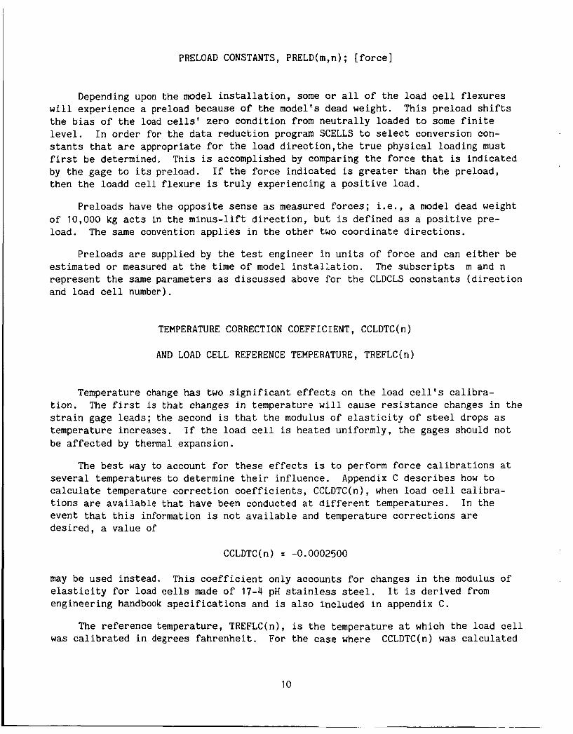
PRELOAD CONSTANTS, PRELD(m,n); [force]
Depending upon the model installation, some or all of the load cell flexures will experience a preload because of the model's dead weight. the bias of the load cells' zero condition from neutrally loaded to some finite level. stants that are appropriate for the load direction,the true physical loading must first be determined. by the gage to its preload. then the loadd cell flexure is truly experiencing a positive load.
This preload shifts
In order for the data reduction program SCELLS to select conversion con-
This is accomplished by comparing the force that is indicated If the force indicated is greater than the preload,
Preloads have the opposite sense as measured forces; i.e., a model dead weight of 10,000 kg acts in the minus-lift direction, but is defined as a positive pre- load. The same convention applies in the other two coordinate directions.
Preloads are supplied by the test engineer in units of force and can either be estimated or measured at the time of model installation. The subscripts m and n represent the same parameters as discussed above for the CLDCLS constants (direction and load cell number).
TEMPERATURE CORRECTION COEFFICIENT, CCLDTC(n)
AND LOAD CELL REFERENCE TEMPERATURE, TREFLC(n)
Temperature change has two significant effects on the load cell's calibra- tion. The first is t ha t changes i n temperature will cause resistance changes in the strain gage leads; the second is that the modulus of elasticity of steel drops as temperature increases. If the load cell is heated uniformly, the gages should not be affected by thermal expansion.
The best way to account for these effects is to perform force calibrations at several temperatures to determine their influence. Appendix C describes how to calculate temperature correction coefficients, CCLDTC(n), when load cell calibra- tions are available that have been conducted at different temperatures. In the event that this information is not available and temperature corrections are desired, a value of
CCLDTC(n) = -0.0002500
may be used instead. elasticity for load cells made of 17-4 pH stainless steel. engineering handbook specifications and is also included in appendix C.
This coefficient only accounts for changes in the modulus of It is derived from
The reference temperature, TREFLC(n), is the temperature at which the load cell was calibrated in degrees fahrenheit. For the case where CCLDTC(n) was calculated
10

from multiple calibrations, TREFLC(n) is the datum temperature used in the calculations.
TARES, PITCH TARES, AND PITCH TARE DATA FILES
PTAR.DAT and TCOF**.DAT
Pitch tares serve the same function for the load cell balance system as the "static" used with the 40 by 80 Wind Tunnel balance system. that can be subtracted from the data to account for shifts in the model's weight vector reiative to tne baiance system after the zeros ai.e taken.
They are a set of tares
Pitch tares are taken during a tare run. The procedure is the same as it is
No external forces are applied to the model as for a normal data run; zeros and rcal points are taken when the model is in the reference position (PTZ and PTC). data are recorded with the PTR command. are a measure of the change in the load cell force readings when the model or parts of the model are changed to positions other than the reference position that they occupy during a zero point.
The data set from a tare point (tare frame)
The tares are sorted by ascending alpha (pitch angle) and stored in the file TCOF**.DAT which can be accessed later to change individual tare values. The ** represents the run number during which the tares were taken. It is possible to make several different tare runs for different model configurations.
When NTAR is set equal to a tare file number, then the tares corresponding to a given alpha in the file will be subtracted from any data with the same alpha. data are being taken at an alpha for which no tare exists, then a straignt line interpolation will be made between the two adjacent tares and that value sub- tracted. tares that the interpolated values will generally be poor.
If
It should be noted that because of the typically nonlinear nature of the
Tares are also subtracted from the preload values to make a first order correc- tion of the interactions that are due to changes in model pitch.
11

TABLE 1 . - LOAD CELL NUMBERING
Load cell 1 2 3 4
Conf igura t ion
Tail s t r u t a f t Left main Right main Tail s t r u t Tail s t r u t forward Tail s t r u t Left main Right main Four load cells Left f r o n t Right f r o n t Left rear Right rear
12
STANDARD 40 BY 80 ATTACHMENT PAD 5 in. BOLT CIRCLE
.-. =k -.
-
i i i i I I 1 1 CONNECTOR
PLUG
' FLEXURE
/ REACT POINT (@i+ FLEXURE
'ION
(a) Three-component load cell.
Figure 1.- Three-axis load cell installation.
13
n 9
\
/
-’ W
(I] 4 4 Q, 0
a (d 0 4
a C (d
(I] c, C
9 . 4
0 a U L (d s 4 (I,
E C Q) Q, 3 c1 Q, D (I] U 8. c, C
3 0 (d c, c, (d
4 a, a 0
h
n v
a 0, 3 C .d c, C 0 u I
c
Q, L 3 m .d crr
1 4

I '
M C
-4 c, *I4 v1 0 a
I
c
15
\ ‘r I c
16
a, L 3 M

29/64 (0.453) 6 HOLES EQU. S.P. REF. ONLY p- 2.000 '1
I
9.00
LIFT-STRUT CLEVIS
I L_I
DRILL
/ 1 .OO BORE "MONOBAL BEARiNG
DlAM B.C.
1 7-
1.500
DlAM
/I c ', 5.75
1 10.5 I
TYPICAL LOAD CELL
I A
LIFT STRUT TIP
SECTION A-A
CLEVIS TO LIFT STRUT CLAMP
Figure 3.- Typical strut to model mounting hardware.
17

Y z -l - n
% v)- l
0 K
Y z -l -
.. w 2 v) Y z -l K w z -l 4
-
a
ou f 5 a
0
v) 0 . 0 . .
Y z -
U
c, m 2 c, m a, &
c 0 .rl u)
7 4 1 a 0 t a & a, 3
I
=r a,

K w K w I I-
a
t w 4 w I I-
& n 0 ~
X
C 0 .rl L)
c
(d U C a, .rl L 0
a, r( M G cd a, >
I
L n
a,
19

APPENDIX A
SAMPLE CALIBRATION REPORT FOR LOAD CELL S.N. 486
(NORMAL FORCE GAGE ONLY)
20

N A S A - A M E S RESEARCH CENTER
3 0 e b
/ / A s h AE/ 4 I 4 8 6 7
INSTRUMENT I D EWTlFlCATlOW M.nuf.cturnr N a m M0d.l Number Serial N u m b
Instrument Description
ce- U L - o d CALlElAllOl O A I A I RtYAlKS
6 fl-kT& 1 c-4- A&+-/ - -
~ _ _ MOFFETT FIELD, CALIFORNIA 94035
> 4-64.h
Calibration Report Number
Previous Service Date Calibration Date
Calibration Interval Next Calibration Due
Contract &umber
847 - 8 % I w. 8 - 1 ? - 8 1
R E A S O l IO8 SUEYISSIOl
0 NOW Instrument
calibration I
CALIBRATION REPORT PACt-OF-
I C A l l E l A f l @ l ACfNcT I Amas Prowrtv Tan Number 1
NOTE: USE ARC l O l A "CALIBRATION REPORT SUPPLEMENT" FOR RECORDING AOOlTlONAL INFORMATION.
YES THIS CALIBRATION WAS PERFORMED WITH "STANDARDS f l TRACEABLE TO THE NATIONAL BUREAU OF STANDARDS.
' L A B O R A I O R Y SUPtRUISOR OISIRIBU~IOI:
NO 0 CONTRACT MONITOR'S COPY .. (WHITE) CALIBRATION FACILITY COPY -- (YELLOW) REOUESTOR'S COPY .. (PINK1
ARC 101 IRev. Jun 75)
Figure A1. - Calibration report form.
21
22
C 0 -4 L, a L, C a, d L 0
0 a a 0 cl

Rut4 #
1 2 3 4
6 7 8 3
18 1 1 12 13 14 1s 16 17 18 19
c J
O j P v 1 V
. 0 0 6 8 19
.88 1755 . DO3488
.nos22 1 . a06940
.808657
.6( 18367
. 8 12876
. 8 13770
.a15612
. 8 13763
.8 12868 . <I 10355 ,088639 .80692 1 . 085 199 .803474 .of31753 .8808 17
LOAD CELL CALIBRATION T . O . NORPlFIL CAGE UNDER POS I T I VE TENS1 ON DATE S E R I A L # E4867 MtlEMOtIICS: NORMAL CFIGE TARE WEIGHT : 0 l b s W E . ROOM TEMP. : 0 DEG. F FULL-SCALE LOAD : 18000 l b r
E X C I T . V 2 V
10.84068 10.8487 1 10.04072 10.84070 10.84869 10.04073 10.84876 18.84073 10.04873 10.84873 10.04870 18.84066 18.84864 18.04865 10.04864 10.04063 10 84862 10.04863 10.04866
( V 1 -vo>jv2 v j v
0.0880000 .080 1729 -0083455
-0066893 .a008603 .80 10306 .08 12008 .80 13695 .00 15530 . O O 13688 .0011992 .88 10294 .0868585 .8006874 .0005 159 ,880344 1 .8001727 -. 8008002
0005181
STD LOAD l b r
0.00 1999.83 3989.66 5981.46 7363.53 9947.47
11925.88 13901.59 15864.67 17989.07 15855.24 13887.62 1 1 928.62 9938.33 7961.08 5974.32 3985.53 2808.44 =. 24
EEST F I T STRFIICHT LIEIE EQCIATION : Y=A(02+A<l)*X
f . ! 6 ? b s r. T .-. k I r. I. r. r. r, r I I T CL T T n L I - a I nitunr u LSC Y A 11 I A V V V - PIFIXIMUM D E V I A T I O N = 15.24 l b s 5 ORF'ELHT I O N COEFF. = 99999828
CALC. LORD l b s
-5.33 1997.32 3996.51 5995.72 7978.77 9959.47
13903.63 15857.83 17982.77 15849.80 13885.27 11918.39 9938.79 7956.89 5970.38 3380.40 1995.83
-7.64
i 1932. e9
: A-387 : 8-1 7-82
DEV. i bs
-5.33 -2.51
6 . 8 5 14.26 15.24 12.80 6 .21 2 . 8 4
- 6 . 8 4 -6 .30 -s. 4 4 -2 .35 -2.23
46 -4 .19 -3.94 -5.13 -5 .41 - 7 . 4 8
ACCU. 2 i F . S . i
- . [I 3 El
-.El14 .938 . 8 i 9 , 0 8 5 .067 .a35 . O i l -. 838 -. 8 3 5 -. 030
- .a13 -. 012 .083 -. 923 -. 022 -. 8 2 8 -. 038
-.rC41
Figure A3.- Loadcell calibration report.
23

LORD CELL CAL I BRAT I ON ttORMRL GAGE IJNOER POS I'T I VE TENS I ON S E R I A L 0 : 4 8 6 7 MNEMOtt I CS: NORMAL GAGE TRRE WEIGHT : 0 lbs
FULL-SCALE LOAD : 1 8 0 0 0 lb, FIVE. ROOM TEMP. : e DEG. F
LOAD CELL CALIBRHTION STD LBS
T.O. :A-387 DATE : 8- 1 7 - 8 2
4
4
4
4
4
4 /'
/"
//- /: .
. 0 ,e' p
cu 1
P
+ S I W 1tIDIi:"TES F I R S T HHLF O F THE LOADING CYCLE
RESISTOR = 108 I( OHMS
RCHL = - . 80@434 V / V NO LOAD V f V RCAL V / V
690003 -. 0 0 0 4 3 1
Figure A 3 . - Continued.
24
SIC PWR - +

Rut4 I
1 2 3 4
d
8 9
10 11 12 13 1 4 15 16 17 18 1%
c J
7
L O A D C E L L C A L I E R R T I O N 1IOF:tIAL GHGE UtIDER t I E G R T I VE T E t I S ION S E R I H L # :4867 I I t I E H r J t I I CC;: t I O R M A L GRCE T H R E LIE I GHT : 0 l b s A'JE. ROOM TEMP. : 8 DEG. F F U L L - S C A L E L O A D : 18088 l b s
p ( C i T . :*2
V
10.84872 18.04873 18.84876 18.04878 18.84077 10.84078 18.04073 18.04874 18.04874 1 0.84878 10. C14872
18,84875 18.84878 10.04865 18.04869 18.04066 18.04066 10.. 04068
18.04c172
<vi-vo j ,y2 v /v
8.0880880 -. 886 1742 -. 0803463 -. 8005198 -. 0886923 -. 0088644 -. 06 18363 -.DO12077 -. 0813793 - .00 15636 -. 0013791 -. 80 12070 -. 09 18353 -. 8805632 -. 0886986 -. G1805187 -. 8883462 -. e08 1736 0.0008000
i i i f i D 1 bs
8.88 -2082.79 -3991.32 -5991.71 -7971.10 -9951.86
-11927.55 - 13896.23 -15855.19 -17973.27 -1 5857.21 - 13886.88 - 1 1918.21
-9343.10 -7958.50 -5976.16 -3388.78 - 1997 SF;
3.12
E:EST F I T S T R A I G H T L I N E E O U A T I O N : Y = A ( O > + A ( 1 ) * X 'I,- I t I T E R C E P T = H ( 0 ) = -4.880040 13483 1 bs S L O P E = A ( 1 ) = 11581852.7826 lbs* ' (V l 'V )
F - T H t I D t i R D D E V I A T I O t 4 = 6.65 1 hs I.lAXII.1UM D E V i A T I O t 4 = 14. 93 1 bs C O R R E L A T I O N COEFF. = .99993852
T.O. :A-387 D A T E :8-17-52
C C i i t . i O f i D GEV. I b s 1 bs
-4.86 -4.88 -2888.25 -5 .46 -3934.44 -3.12 -5982.90 -1.1% -7966 80 4 . 3 8 -9946.10 5.76
-11923.18 4 .37 - 13334.47 1.76 - 15568.06 -2.87 - 17988.20 -14.93 -1=*.- d.3b5.80 -e. 5 % -13886.48 . 3 2 -11911.78 6.51
-9932.44 18.66 -7947.42 11.08 -5478.35 5.81 -13986.46 2 .32 -2681.40 -3.24
-4.88 -8.08
.-c A I I
H C . L U .
Y ( F . 5 . )
- . 8 2 7 -. 8 3 8 - . O l i -. 007 ,024 , 0 3 2 . Q 2 4 .010
- .816 -. 883 -. 1345 . ElilZ , 0 3 6 . a 5 9 .862 . Kl 'Z 2 ,013 - . 9 2 1 -. 0 4 4
Figure A 3 . - Continued.
25

STD 3888
0
-2800
-4888
-6008
-8888
- 180QQ
- 12880
-14880
-16000
- 18888
LORD CELL C R L I E R R T I O N tlr3RPlRL GAGE Ut4DER NEGRT‘I VE TEtJS I ON SERIRL 0 :4867 MtiEPlOt4 I CS: NORMAL GRGE THRE WEIGHT : 8 I b s HVE. ROOM TEMP. : 0 DEG. F FULL-SCRLE LOAD : 18000 I b s
T.O. :A-387 DATE :8-17-52
LOAD CELL CALIBRflTION LBS
b
4
4 4
b
* 4
* b
4 4
b
S I G N I14DICHTES F I R S T HRLF OF THE LORDING CYCLE
RESISTOR = 180 K OHMS NO LOAD V/V RCAL V/V - . O m 4 3 1 RCAL = - . I388434 v / v . 0088e3
SIC PWR - +
Figure A 3 . - Continued.
26

RUN #
1 2 3 4 5 t. - 8 9 10 1 1 12 1 3 14 15 16 17 i 3 1 9
BE$.
INTERACTION NORMAL GAGE UNDER P O S I T I V E TENSION S E R I A L 0 :4867 MtlEMON I CS : AX I AL CAGE TARE WEIGHT : 0 l b s W E . ROOM TEMP. : 0 DEC. F FULL-SCRLE LOAD : 6088 l b s
E X C I T . V Z v
10.83750 18.03752 10.83752 18.03751
10.03755 10.83757 10.03753 10.03754 10.83754 18.83751 10. 63745 10.03743 10.03745 18.03744 18.83743 1 8 . 03743 10.83744 10.03747
10.03748
~ V l - V o > / V 2 V/V--> 1 bs
0.00 -3.08 -3.70 -1.85 -1.85 -1.23 -2.47 -3.08 -4.93 -6.17 -6.17 -4.93 -3.70 -2.47 -1.85
- . 62 -1.23 -.62 - . 6 2
F I T STRAIGHT L I N E EQUAT t~ : Y = A ( 0 '.i '-ItITEPCEf)T = A i @ ) = -.40095693028 l b s SLOPE = A(1) = -2.66619280428E-04
STD LOAD l b s
0.00 1999.83 3989.66 5381.46 7963.53 9947.47 11925.88 13381.59 15864.67 17989.07 15855.24 13887.62 11920.62 9938.33 7961.08 5974.32 3985.53 2880.14 -. 24
T.O. :A-387 DATE : 8- 17-82
CALC. LOAD l b s
-. 40 -. 93 -1.46 -2.00 - 2 . 5 2 -3.05 -3.58 -4.11 -4.63 -5.28 -4.63 -4. le -3.58 -3.05 -2.52 -1.99 -1.46 -.33 -. 40
DEV. l b s
-. 48 2.15 2.24 -. 15 -. 67 -1.82 -1.11 -1.02
.30
. 9 7 1.54 .23 .12 -. 58 -. 67
-1.38 -.23 -.32 .22
fiCCI). % ( F . S . )
-. 807 ,036 .837 -. 602 -. 81 1 -. 830
-.014 -.017 .805 ,816 .a26 .014 .a02
-.010 -.011 -. 823 -. 804 -. 085 .084
!5THt4DHF.:D DEVIHTIrJI4 1 . 10 1 bi l4 f iXIPlUM D E V I H T I O N = 2.24 l b s CORRELHT I OtI COEFF. = .63831363 V / V CONVERTED TO LBS BY USING IST-DEC SLOPE
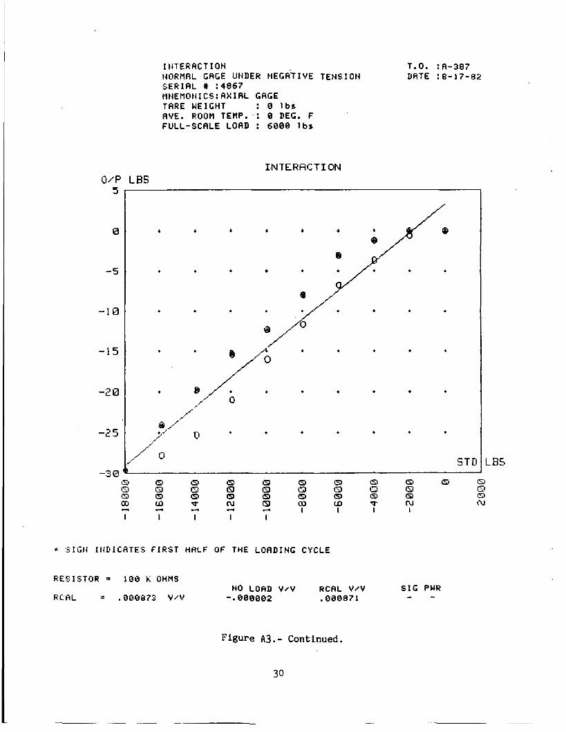
Figure A3.- Continued.
27

INTERACTION NORMAL GAGE WIDER POS I T I’VE TENS I ON SERIHL 0 : 4 8 6 7 Mt4EMON I C s : AX I AL GHGE TARE WEIGHT : 0 l b s
FULL-SCALE LOAD : 6880 1bS AVE. ROOM TERP. : 8 DEC. F
T.O. : A - 3 6 7 DATE :8-17-82
I N T E R A C T I O N O.’P LBS 0
- 1
-2
-3
-4
-5
-E
-7
4 b 4
8 0 0
0
0
STD
+ S1Gt.I It4DICFtTES F I R S T HALF OF THE LOADING CYCLE
RESISTOR = 100 K OHMS
f7I::fiL = .FJ88873 v j v SIG PWR - NO LOAD V / V RCAL V / V - -. twe002 . e0087 1
Figure A3.- Continued.
28

RClN #
1 2 3 4 5 6
3 9
10 11 12 13 14 15 16 17 18 i ?
T
I EITERACT I ON tIOP.11HL GHGE UtIDER tIEGAT'I VE TENS I O N S E R I A L # :4867 MIIEMON I CS : A X I AL GAGE TARE WEIGHT : 0 l b s
FULL-SCALE LOAD : 6009 l b s AVE. ROOM TEMP. : 0 DEG. F
T.O. :A-387 DATE :8-17-82
E X C I T . V 2 V
18.83755 10.03755 16.83757 19.83761 18.83758 1 0 .a3759 1 0.83753 10.83753 18.83755 10.83759 10.83752 10.83755 10.03756 18.03751 10.83747 10.03748 18.83748 19.83746 18.83750
< v 1 -vo ) /V2 V/V-- > 1 bs
0.60 0.00
-1.23 -3.88
-12.33 -15.42 -19.73 -24.05 -29.60 -27.75 -25.28 -20.97 -16.03 -11.72
-6.78 -3.70 -. 62
. 6 2
-e. e2
STD LOAD l b o
0.80 -2802.79 -3991.32 -5981.71 -7971.10 -9951. B6
-1 1927.55 - 13896.23 -15865.19 - 17973.27 -15857.21 - 13886.80 -1 1918.21
-9943.10 -7958.50 -5976.16 -3988.78 -1997.56
3.12
CALC. L o r n l b s
3.35 -. 25 -3.82 -7.39
-18.97 -14.53 -18.88 -21.61 -25.15 -28.94 -25.14 -21.66 -18.06 -14.51 -10.95
-7.38 -3.81 -. 2 4 3.36
DEV. l b s
3.35 -. 25 -2.58 -4.31 -2.95 -2.19 -2.66 -1.88 -1.19
. 6 G 2.61 3.69 2.91 1.52
.77 -. 60 -. 11
. 38 2.74
ACCU. X < F . S . )
, 856 -. 004 -. e43 -. Q 7 2 -. 049 -. 037 -. 0 4 4 - . 0 3 1 - . o l e
.011
. 8 4 4 . 861
.048
. 8 2 5
.013 - . @ l e -. 082
.0f36 fi 'i . v 4 0
BEST F I T 5TRAIGHT L I N E EQUATION : Y=A(B>+R( 1 ) * X ' i ' - I t lTERCEFT = A ( 8 ) 3.3528827095 l b s SLOPE '= A(1) = 1.79658117858E-03 < l b r ) / < l b o )
CTG!!Ef i tE pES'!2T!g!.! !z -. 3 13 - - ?I%%
b1FI:X I PIUM DEV I AT I ON = 4 e 3 1 1 bS CORRELHTION CUEFF. = .94711418 V/V CONVERTED T O LES BY USING 1ST-DEC SLOPE
Figure A3. - Continued.
29
I tlTERACT I O N tlORMAL GAGE Ut.lDER EIEGA'T I VE TEHS I ON SERIAL # :4867 Mt IEMOt l ICS: A X I A L GAGE TARE WEIGHT : 0 lbs AVE. ROOM TEMP. : 9 DEG. F FULL-SCALE LORI) : 6000 l b ,
I N T E R A C T I ON LBS
T . 0 . : A - 3 8 7 DATE : 8- 17-82
b b 4 b
. . 0
.
-38
d 4 d d I I I I I I I I I
+ SIGH It(D1CATES F I R S T H R L F OF THE LOADING CYCLE
RESISTOR = lo@ K OHMS
RCHL = .E188873 v /v -. 008002 .08087l - - HCAL v /v SIC PWR NO LOAD V / V
LB5
Figure A3.- Continued.

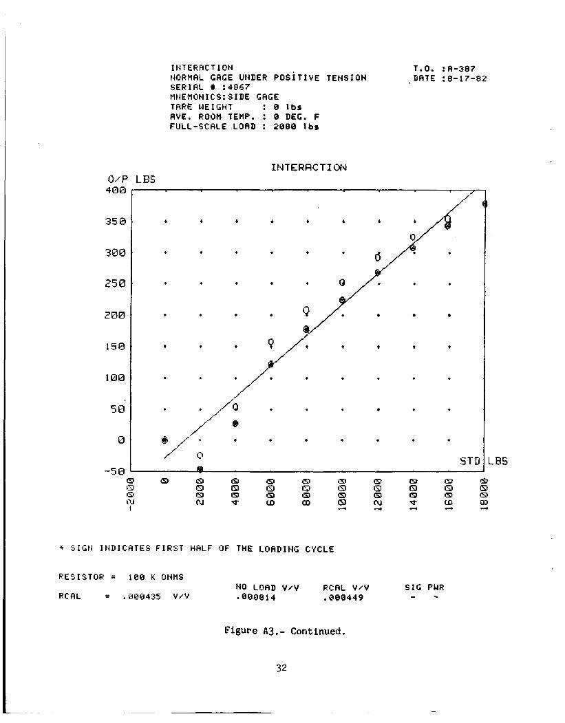
I t4TEEACT I ON NORPlAL GRGE UNDER P O S I T I V E TENSION S E R I H L # :4867 HHEMtrNIL'S: SIDE GAGE TARE WEIGHT : 8 lbs AVE. ROOM TEMP. : 0 DEG. F FULL-SCALE LOAD : 2000 l b s
T.O. :A-337 DHTE :8-17-82 ,
PL1t.I # O i P '41 EXCIT .V2 <Vl-V0)/V2 STD LOAD CALC. LOAD DEV. ACCU. V V V/V- - > 1 bs l b s l b r 1 bs Z ( F . S . >
1 2 3 4 5 6
8 9
18 11 12 1 .I: 14 15 li 17 18 19
-
10.03684 10.83605 10.03602 18.83683 18.03608 10.03586 18.43610 10.03607 10.83603 18.83688 10.83605 10.03538 10.03596 18.83596 10.03536 19.83536 10.03596 10.03596 1 0 . 0 3 5 9 7
0.80 0.00 -43.83 1999.83
27.08 3939.66 122.15 5381.46 178.18 7963.53 224.63 9947.47 267.55 1 1325.85 308.87 13981.59 343.57 15864.67 378.27 17989.07 354, %0 15855.24 325.72 13887.62 292.03 11920.62 2J2.32 9938.33 208.19 796 1.08 158.25 5974.32 53.95 3985.53
-24.24 2008.44 -. 22 -. 24
-29.87 -2s. 137 -1 .453 20.30 66.13 3.306 69.42 42.34 2.117
118.59 -3.56 -. 178 167.52 -18.59 -. 529 216.49 -8.14 -. 407 265.33 -2.23 -. 111 314.10 6.133 - 3 8 1 362.56 18.99 .?49 415.80 36.73 1.537 362.32 7.72 .?86 313.75 -11.97 -. 598 265.20 -26.83 - 1.342 216.26 -36.05 - 1.803 167.46 -48.73 -2.037 118.41 -39.84 -1.992 69.32 15.36 .768 28.32 44.55 2.228
-29.87 -28.85 - i . 4 4 3
E:EST F I T 5TRHIi;HT L I t I E EOUATION : Y=A(B)+ACl )*:< '1'- I tITERCEPT = A 0 > -29.86622 1642 1 bS 5 LOP E 2. +w52796759E-82 < 1 b s ) # ' < 1 b r
- - - . . - - r s - - . . - --. -,. ..-. -.. . L - 7- I nr+unr u i i t v 1 n I I IJIY = 221.35 IU,
1.1,5>iINL~Pl DE'4IHTION = 66. 13 1 bs LOPRELAT I O t I COEFF. = .95187423 V / Q CONVERTED TO LBS BY USI t IG 1ST-DEG SLOPE
Figure A3.- Continued.
31
INTERHCTION t4rJRMAL GAGE UtiDER POS 1 T I VE TENS I ON S E R I A L 0 :4867 MtlEMON I CS: SI DE GHGE TRRE WE I GHT : 0 l b r AVE. ROOM TEMP. : 0 DEG. F FULL-SCALE LOAD : 2080 Ibr
ZNTERACTION W P LES 4 0 0
358
380
250
ZQB
150
1 OQ
5 0
8
-5 0
1.0. :A-387 DATE : 8- 17-82
/’
* * t t
. . 0
0 0
0 . 0
STD
* 5 I G t . I I t 4 D I C A l E S F I R S T HALF OF THE LOADING CYCLE
RESISTOR = 188 K OHMS SIG PUR 140 LOAD V / V REAL v / v
RCAL = .ir88435 v / v *0@0814 .$BO449 - -
I
LBS
Figure A3.- Continued.
32

Riii.i %
1 2 3 4 5 6
8 4
10 11 12 13 14 1.5 16 17 18 13
7
I tlTERRCT I ON tIORP1AL G A G E Clt4DER t4EGRTIVE TENSION S E R I R L 0 :4867 MNEMON I CS: S I DE GRGE TRRE ME I GHT : 8 lbs AVE. ROOM TEMP. : e DEG. F FULL-SCALE LOAD : 2800 lbs
T.O. :R-387 PATE : 8- 17-82
-..*-- . . A
C A L I I . Y L
V
18.03687 10.83687 10.0361 1 18.83615 10.03612 18.0361 3 18.83686 18.83686 18.83688 18.83612 18.836:87 18.83687 10.83688 18. a3686 10.83680 18.836134 18.83603 18.03601 19.83603
0.90 56.96
147.22 228.24 380.25 362.82 410.36 446.26 471.73 478.35 443.25 407.55 365.43 316.49 259.53 194.35 118.54 45.13
5.01
n v F. I 3 1 Y L V ~ Y
lbs
8.08 -21302.79 -3991.32 -5981.71 -7971.10 -7951.86 - 11 927.55
- 13896.23 -15865.19 - 17973.27
-13886.80 -1 1418.21
-9943.10 - 7 9 5 8 . 5 0 -5976.16 -3988.78 - 1997: 56
3.12
-15857.21
21.62
136.73 194.14 251.52 388.65 365.63 422.41 479.28 548.00 478.97 422.14 365.36
251.15 193.98 136.66 79; 23 21.53
79.38
'308.39
l..l-l, Y C Y .
1 bs
21.62 22.42
-18.48 -34.18
-53.37 -44.73 -23.85
7.47 61.65 35.72 14.59 -.07
-8.18 -8.38 -. 37
: 3 4 . 1 8 16.51
-48.73
18.12
,-. C. p. I I n L. 1-1 . 2 ( F . S . )
1.881 1.121 -. 524
- 1.705 -2.436 -2.669 -2 .237 -1.193 . 3 i 3 3.053 1.726
.729 -. 004 -. 405 -. 419 -. 018
.906 1.705 .126
BEST F I T STRAIGHT L I N E EQURTIOt4 : ' I ' = A < 8 ) + A < 1 ) * X ' I ' - I t lTEPCEPT = A ( , O ) = 21.615815649 l b s SLOPE = A < l ) -.028841871425 (lbs)/<lbs)
STHtlDF1RD D E V I A T I O N = 30. 16 1 bs P1A:;IElUM D E V I A T I O N = 61.65 lbs CORRELAT I ON COEFF. = . 9 6 4 6 w a V / V CONVERTED TO LBS B ' I USING LST-DEG SLOPE
Figure A3.- Continued.
33

INTERRCTION NORMAL GAGE UNDER NEGAT i V E TENS I ON S E R I A L # :4867 MNEPIONICS: S I D E GRCE TARE WEIGHT : 8 lbs AVE. ROOM TEMP. : 0 DEG. F FULL-SCALE LOAD : 2000 l b 8
T . O . : A - 3 8 7 DATE : 8 - 1 7 - 8 2
I N T E R A C T I O N O/P LB5 580 -
P 'b 4 5 0 IJ \\., 8r
408
358 b b 4
308 . 9
I d
I Z 5 Q
2r30
150
180
*
.
b 4
.a
I
I * \
b b b 4 b b O\ <. 1
I ' *
I \ STD
d 4 4 4
I I I 1
Q 8 m . (D
I v-
* S I L N INJDIC'ATES F I R S T HALF OF T
RESISTOR = 180 K OHMS
RCHL s .000435 V / V
IE ORDI..T; C'
NO LOAD V / V .0000 1 4
LBS
C
RCAL V / V . 0 8 0 4 4 9
E
Figure A 3 . - Continued.
34

I t4TERACTION t4CJRMAL GAGE UNPER + & - TENSION SEf?IHL # :4867 MNEMOH I CS: S I DE CAGE HVE. ROOM TEMP. : 0 DEG. F FULL-SCALE LOAD : 2000 l b s
E X C I T . V2 V
10.03604 10.83685 10.83662 18.83683 10.03680 18.03606 10.83610 10.83607 10.83688 10.03608 10.83685 14. 8.3598 18,83536 18. C135'36 10.83596 18.83596 10.83536 18.63596 10.83547 10.08687 18.8:3687 18.8361 1 10.83615 18.83612 18.03613 10.83606 10.03606 10.83688 18.0361 2 10.83607 n n:?gn7
._ 10.83688 !. 18.83686
18.03600 18.03684 10. 03603 19.83601 18.03603
( V 1 -Vo ) /V2 V/V-- > 1 b r
0.00 -45.83
27.08 i22. is 178.10 224.63 267.55 388.07 343.57 378.27 354.60 325.72 292.03 252.32 208.19 158.25 53.95
-24.24 -. 22 0.88
56.96 147.22 228.24 300.25 362.02 418.36 446.26 471.73 478.35 443.25 407.55 365.43 316.49 259.53 194.35 118.54 45.13
5.01
STD LOAD I b s
8.80 1999.83 3989.66 5481.46 7963.53 9947.47
11925.88 13901.59 15864.67 17789.07 15855.24 13887.62 11928.62 4938.33 3961.08 5974.32 3985.53 2000.44
-.24 0.80
-2t382.79 -399 1 .32 -5981.71 -'971.10 -99s 1.86 - 1 1927.55 - 13896.23
-15865.19 -1 7973.27 -1 5857.21 - 13886.80 -1 1918.21
-9943.10 -7958.50 -5376.16 -3988.78 -1937.56
3.12
CALC. LOAD l b r
T . O . :A-387 DFtTE 8- 17-82
223. 18 214.81 286.47 i 9 8 . i 3 189.83 181.52 173.24 164.96 156.74 147.84 156.78 165.82 173.26 181.56 189.84 198.16 206.49 214.88 223.18 223.18 231.57 239.40 248.23 256.56 264.86 273.13 281.38 289.62 298.45 289.59 281.34 273.03 264. $2 256.51 248.21 239.89 231.55 223.17
DEV. 1 bs
223.18 260.63 179.40 (3.88 11.73
-43.11 -94.32
-143.11 -186.83 -230.43 -197.82 -16c3.70 -1 18.77
-70.76 -1s. 35
39.91 152.54 239.04 223.40 223.18 174.61 92.68 19.99
-43.68 -97.16
-137.23 -164.88 -182.11 -179.89 -153.66 -126.21
-92.34 - S 1.67
-3.02 53.86
121.35 186.42 218.15
--
ACCIJ. 2(F. S. )
11.159 13.032 8.970 3.749
. 5 8 6 -2.156 -4.716 -7.155 -9.342
-1 1.521 - 9 . 5 9 1 -8. B35 -5.939 -3.538 -. 918
1.996 7.627
11.452 11.178 11.159 8.738 4.634 .439
-2. -4.858 -6.861 -8.244 - 4 . 1 0 5 -8.995 -7.683 -6.31 1 -4.617 -2.584 -. 151
2.693 6.068 9.321
i o . 908
BEST F I T STRHIGHT L I H E EQUATION : Y=A(0)+A(l)+X ' i * - I t ITERCEPT = A ( @ ) = 223.1809461 l b , SLOPE = A ( 1 ) = -4.188018046326-03 < l b s ) / C l b s )
STHtlDHRD DEVIHTIOtJ = 149.94 l b s P1HX IPIUM DEV I AT I O N = 260.63 1 b s GORRELAT I O N COEFF. = .07352824 V / V CONVERTED TO LBS BY USING 1ST-DEG SLOPE
Figure A3.- Continued.
35

I t1TEPACT I O t 4 t1ORMAL GAGE UNDER + & - TENSION S E R I A L # :4867 lIt4EIlOt4ICS: S I D E GAGE FIVE. ROOM TEMP. : 8 DEG. F FULL-SCALE LOAD : 2888 1bS
I N T E R A C T I O N 0,'P L R S
0 8 0 0
b
.
.
0
8
0
0 0
8 0 0
STU
T . O . :A-367 DATE : 8- 17-82
J
1e5
S I C PWR - t.10 LOAD V / V RCAL V /Q . 0@8@ 14 .088449
Figure A3. - Concluded.
36

APPENDIX B
JET PROPULSION TEST STAND
LOAD CELL-LINK INSTALLATION
8 . To i n s t a l l t h e one-Ax LC l i n k s , remove a l l s o l i d l i n k s t h a t are used t o t r a n s - p o r t and store t h e test s t a n d . The balance table to which models are a t t a c h e d should be r e s t i n g on f o u r screw snubbers . f o u r and have a corresponding gage block. The snubbers are a d j u s t e d by t u r n i n g t h e screw u n t i l the d i s t a n c e between the tabie a n a t h e snubber base are e q u a i t o the a p p r o p r i a t e gage block, f i g u r e B1.
The snubbers are each labeled from one t o
With the snubbers a d j u s t e d , i n s t a l l the v e r t i c a l load l i n k s . I t is important n o t to p r e l o a d t h e l i n k s d u r i n g t h i s phase of t h e i n s t a l l a t i o n as it w i l l cause misalignment t h a t can r e s u l t i n load measurement errors. The b e s t way t o avoid p r e l o a d s is t o connect t h e load ce l l s t o a d a t a a c q u i s i t i o n system and monitor t h e i r o u t p u t d u r i n g load cell i n s t a l l a t i o n . The l i n k s are assembled as shown i n f i g u r e B1 us ing t h e fo l lowing s t e p s :
1 . Assemble the load ce l l l i n k as shown b u t l e a v e a l l jam-nuts loose. Make s u r e a l l washers, n u t s , and t h r e a d s are l u b r i c a t e d .
2 . T ighten the rods i n t o t h e load c e l l by hand u n t i l t h e t h r e a d s bottom o u t .
3 . Tighten t h e jam-nuts a t t h e top of t h e assembly. The s p h e r i c a l washers allow the l i n k t o a l i g n wi th t h e lower hole i f t h e n u t s are t i g h t e n e d smoothly. With t he upper n u t s t i g h t e n e d , t h e ioad ceii should rotate freely by harid i f iio p a r t s are b inding .
4. Rotate t h e load ce l l u n t i l t h e upper rod is backed o u t a half t u r n from t h e bottom. Loosen t h e lower rod a h a l f t u r n from being bottomed o u t from i n s i d e the load cel l .
5. The load ce l l o u t p u t should now be about z e r o . Tighten one o f t he lower n u t s u n t i l t he monitor reads approximately 50 t o 100 l b . Tighten t h e remaining n u t as t i g h t as p o s s i b l e (nominal 200 f t - l b ) .
6 . With a l l four n u t s t i g h t e n e d , the load c e l l o u t p u t should r e t u r n t o z e r o and t h e load ce l l should a g a i n rotate f r e e l y by hand. t h e o u t p u t of t h e o t h e r load cells. If t h i s is n o t t h e case, e i t h e r an a x i a l or la teral p r e l o a d e x i s t s i n the l i n k . I t is t h e r e f o r e necessary t o loosen a l l t h e n u t s of t h e l i n k t h a t is being i n s t a l l e d and r e p e a t s t e p s 2 through 6 .
There should be no change i n
7. Repeat s t e p s 1 through 6 f o r the remaining v e r t i c a l and h o r i z o n t a l load 1 inks .
37

8. When a l l the necessary load l i n k s have been i n s t a l l e d and are i n d i c a t i n g no loads , screw the snubbers down as far as p o s s i b l e . t i g h t e n t h e snubbers i n their lowest p o s i t i o n . has caused the snubbers to t u r n u n t i l they make con tac t w i t h t h e ba lance table and s p o i l t he data.
I t is a good idea t o secu re ly On occas ion , test s t a n d v i b r a t i o n
38

I A nfi MI IT@ UMWI I Y U I O
TEST STAND PLATFORM
+ LOADCE LL w , / BALANCETABLE
- - -
m FLAT WASHER
Figure B1.- Propulsion stand loadlink installation.
39
-

APPENDIX C
SAMPLE CALCULATIONS
PRIMARY CONVERSION CONSTANTS, CLDCLS(s,m,n); [force/counts]
Assuming that load cell S.N. 4867 is designated number 2, then for the data presented in appendix A, n = 2 and m = 3.
Given typical load cell signal conditioning--excitation 10 [VI, voltage amplification 1000 [v/v], RMDU analog-digital gain 3333 [cts/v], AMX/RMDU gain 1 [cts/cts]--and noting that the sign convention that is used by the RQ & A lab (appendix A, page 14) is opposite that used by the data reduction program, we use the slope from the data on page 17 of appendix A for the positive loading conversion constant, s = 1. From page 17:
Primary conv. = 11501052.0 [lbs/(v/v)]
then
11501052[lbs/(v/v)l 10[v]1000[v/v)3333[cts/v]l[cts/ctsl CLDCLS(1,3,2) =
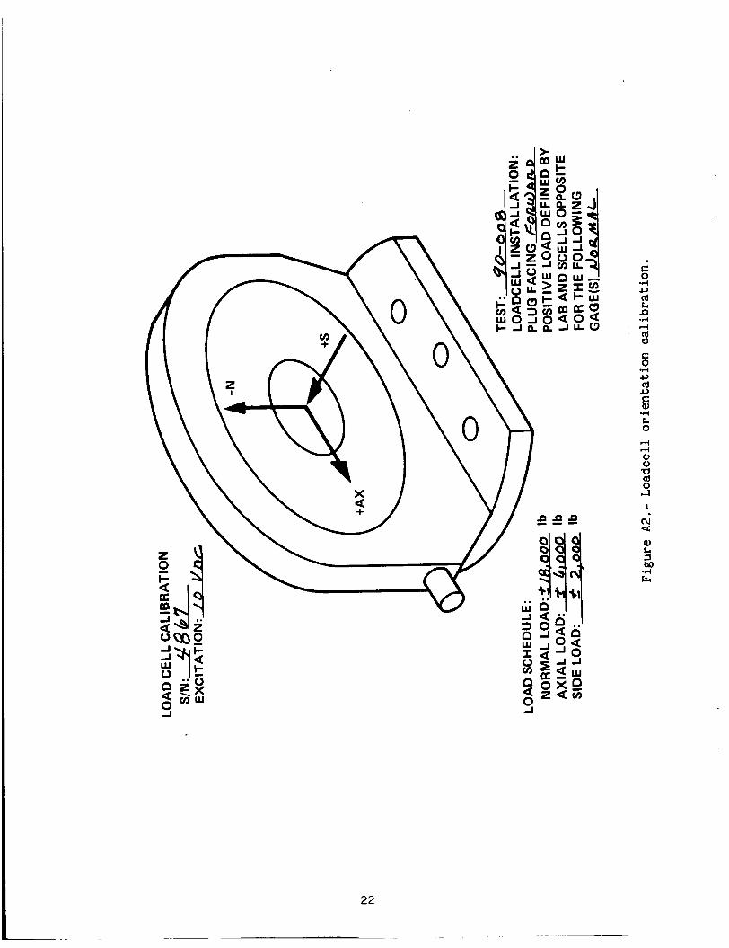
We will devote some space here to say a few words about how positive loads are defined. When the lab technicians calibrate a three-Ax LC, they have no idea what the orientation of the load cell will be when mounted on the model. As a result, when the sense of the positive loads are selected as shown in the figure on page 14, they are completely arbitrary. It is up to the test engineer to determine whether or not the positive loadings shown in the lab calibration are consistent with what is assumed to be positive in the load cell data reduction.
As an example we will use the figure on page 14 and assume that the load cell will be mounted on the model with the bolt-circle up and with the electric plug forward. A drag force on the model (positive axial force) will push the load cell back. Since the pin is restrained, the load cell sees a pull on the pin in the direction of the electric plug. This implies that positive axial force is the same for both the model and the lab. On the other hand, lift on the model (positive normal force) will pull the pin away from the bolt circle which is the opposite of the lab definition. force is the same for the lab and the model.
Using the same reasoning, it can be shown that positive side
40

LABORATORY RCAL VALUES, XINCAL(m,n); [counts]
From page 16 of appendix A:
rcal = -O.O00434[v/v]
since
XINCAL = rcal*excitation*gains
then
XINCAL[ C~S] = -0.000434[ v/v]* 10[ V] * 1000[ V/V] "3333 [ C~S/V I
= -14,465
note that the lab has indicated the use of the negative signal and positive power terminals for recording rcal. would result in a sign change for XINCAL.
The present 40 by 80 convention is to use ++. This
INTERACTION CONSTANT, DSDN(s,n)
If the interaction slopes are given in units of (v/v)/lb, it will be necessary t o multiply this value by the primary conversion constant [lb/(v/v)] of the gage reading the apparent force. s h p e can be read directly from the calibrat,ion in (lb/1blt see appendix A, page 24. constant. Care must be taken to account for any reversals of sign conventions, as discussed above, when assigning specific values. As before, for the data provided in appendix A, the n subscript equals 2 and the s subscript indicates the sense of the loading for the gage experiencing the load.
Often the RQ & A lab has already done this and the
Once the slope is in these units, it can be used for the interaction
From page 24 we have:
DSDN(2,2) = 0.024685 (lb/lb)
This is the interaction for change in side force at load cell 2 that is due to changes in normal force when the normal gage is being loaded in the negative direc- tion. We use data from the lab's positive loading of the normal gage because of the reversal of the assumed positive direction.
It is a good practice to check the significance of the interactions before inserting them into the data reduction. effect on the data. their face value. For example, the coefficient listed above gives the change in side force that is due to changes in normal force but says nothing about how that quantity compared with expected side force measurements.
Interactions of less than 0.1% will have no It is not possible t o tell the significance of interactions by
An easy way to make that
41

comparison is to multiply the interaction coefficient by the ratio of the maximum expected force on the influencing gage Over the expected force on the influenced gage. For a typical model using this load cell: maximum normal force 10,000 lb, maximum side force 2,000 lb
NormMax
SideMax Significance = DSDN"
= 0.0246" lo 2:ooo Oo0 = 0.123 = 12.3%
TEMPERATURE COEFFICIENT, CCLDTC(n)
To calculate the temperature correction for a given load cell, it is necessary to have calibration data for that load cell taken at several different ambient temperatures. The coefficient is a linear interpolation of the data that scales the primary conversion constants as a function of the difference between the load cell temperature and a datum temperature.
The coefficients are determined as follows, given:
TREF
T
AT
CLCTRE F
CLCT
FT
%ts
an arbitrary datum reference temperature
the measured load cell temperature
laboratory constants TREF and used as the inputs for the load cell data reduction program SCELLS
CLDCLS(s,m,n) acquired at an ambient temperature of
laboratory constants ture T
CLDCLS(s,m,n) acquired at some non datum tempera-
load applied to the load cell at temperature
load cell output in computer counts
T
the uncorrected load is calculated by
F~~~~ = CLCTREF*Fcts
42
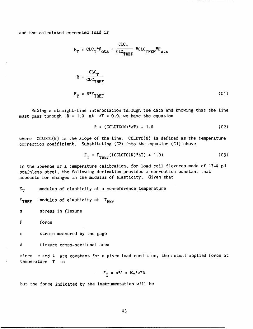
and the calculated corrected load is
CLC, 1
FT = CLCT*Fcts = CLCTREF *CLCTREF*Fc ts
CLCT
C L C ~ ~ ~ ~ R =
Making a straight-line interpolation through the data and knowing that the line must pass through R = 1.0 at AT = 0.0, we have the equation
R = (CCLDTC(N)*AT) + 1.0 (C2)
where CCLDTC(N) is the slope of the line. CCLDTC(N) is defined as the temperature correction coefficient. Substituting (C2) into the equation (Cl) above
( (CCLCTC(N)*AT) + 1 .o) (C3) F~ = F~~~~
In the absence of a temperature calibration, for load cell flexures made of 17-4 pH stainless steel, the following derivation provides a correction constant that accounts for changes in the modulus of elasticity. Given that
ET
E~~~~
S
F
e
A
since
modulus of elasticity at a nonreference temperature
modulus of elasticity at TREF
stress in flexure
force
strain measured by the gage
flexure cross-sectional area
e and A are constant for a given ,oad condition, the actua- appliec force at temperature T is
FT = s*A = ET*e*A
but the force indicated by the instrumentation will be
43

*e*A F~~~ = E~~~
taking the ratio and applying equation (3)
- - - - ET FT F~~~~ - E~~~~
- (CCLCTC(N)*AT) + 1.0
from the Mil. Spec. handbook for 17-4 Ph S.S.
100% at 80°F
92% at 400°F
E~~~~
ET
so
or
CCLCTC ( n ) = -0.000250
Load cells that are operated at elevated temperatures often experience signifi- cant zero shifts. When increased temperatures are encountered, check zeros at the end of the run.
44

OF P P R pfilm Abreviat9-S: M = NIGAGES. (gage no.) - N DCLS (loadcell no.)
FLC (N,M) - FLDCLS (M,N) (gage forces) . Gage output [ lbe] r -\FLC(M,N) = FRGAGE(M,N) I
to local array
Check for pitchtare frame
Read in pitchtare table if not in memory
IF (1PRTYP.NE.IPTFRM l L l Should tare correction be applied to preloads. If so IPTARC = 1
I
I Preload tare corrections I CALL SCLCTR (N,M,ALFDEG,PRELD,PRELDT) I Equate preload arrays PF~ELDT-~ I
I I
Temperature correction CALL SCLCTC (N,M,CCLDTC,TREFLC,THERMO,FLC)[
Interaction correction I LCALL SCLCIA (N,M,PRELDT,DADN ... DSDN,FLC,IERR)~ I
Store pretare forces I I FRCBTR(N,M) = FLC (N,M)[
Check for pitchtare frame again
Record pi tchtarcs CALL SCP'FR ( ALFDFG , FLC , LLUPTF , LUNYRR, IERR)
Should tare correction be applied. If so ILTARC = 1
Farce tare corrections
S t o r e after tare forces
Rotate lcaPcell forces Into body axes
I
I [ FLCATR(N,M) = FLC (N,M) I
I
C m p u te aerodynamic CALL SCLCAF (N,FLC,XYZLCY,FRCBDY)[ forces and moments f
FP.CT)PY, FRCSTB , FRCWND) Qotate forces into the wind and stability axes
Figure C1.- Flow chart for SCELLS (called by SCOMPS).
45

FLOWCHART FOR SCPTRD (called by SCELLS)
Transfer of logical unit number f o r the ?!evice containing the TCOF--.DAT files
Check if the correct tare files are in memory
Open the device
Read the tare tah?e TCOF--.DAT correspondinq to Y W R = -- for tare alphas an? forces
c!.ose device
Return to SCELrIS
LUNTCF , LUNERR, IERR * IF (NTAR. EC. IPTSET) CL1
I
READ fP'I!Al,F ( I) ?TARE(M,N, 1)
CLOSE LUNTCF
\ -
FLOW CHART FOR SCLSTR (called by SCELLS)
Pass alpha, uncorrected forces ani' returns corrected forces
Look up proper tares CALL SCPTLU (N,M,AL?HA,FPTARE)
( N , M , ALPHA, GAGELC , GAGETR ) t
Tare subtraction
Return to SCELLS <=[TGziq
Figure C1.- Concluded.

APPENDIX D
PROGRAM DESCRI PT ION
LOAD CELL FORCE COMPUTATIONS
This appendix describes the computational methods used for the calculation of forces and moments from load cell data. For more detailed information see the actual program listings of the subroutines named. These routines are part of the Ames "Standard Wind Tunnel Software" and can be obtained from NASA programmers or NASA contractor programmers (informaticsj.
There are two independent sets of software that can compute loads. The soft- ware that performs the on-line calculations during actual running is referred to as the "real-time" program, whereas the program used to reduce the data after a run is called the off-line program. Most subroutines in the off-line program are dupli- cates of the software in the real-time program; however, in some cases simplified, but equivalent expressions are used in the off-line program.
Prior to any manipulation of data by the so-called "Load Cell Program" SCELLS, the acquired data in the form of machine computer counts is converted into engineer- ing units (eu). These computations are performed in real-time by the standard wind tunnel conversion routines "SCNVRT" which in turn calls "SCTHRB. '' In the off-line program, the calculation uses the "LOADS" subroutine.
SCNVRT: Standard Conversion Routine
This subroutine determines the type of data that needs to be converted (pres- sure, force transducer, temperature, etc.) and calls the appropriate conversion routine. The subroutine that is called for strain gage balance data is SCTHRB.
SCTHRB: Standard Conversion for Thermal Balances
The SCTHRB subroutine contains several options for the conversion of strain gage balance data into engineering units. Its capabilities include (n)th degree bidirectional polynomial conversions, thermal adjustments, resistance calibration, and bias offset corrections. In practice, the load calibration of load cells is linear to within the accuracy of the experimental facility's data system. For this reason only the first-order "thercal" portion of the subroutine is used. If the researcher feels that a higher order fit of the calibration data is justified, that software can be made available upon request. handle second-order effects such as "interactions," a separate subroutine has been supplied for that case.
Although this feature could be used to
47
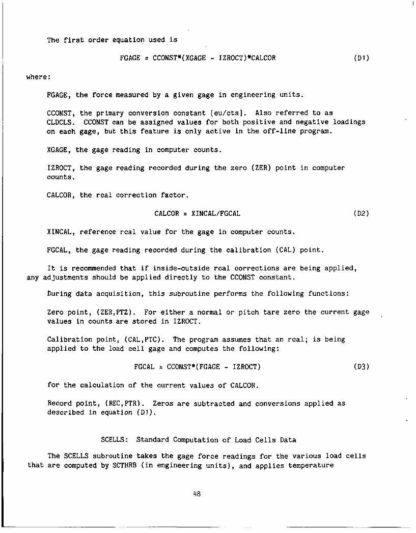
The first order equation used is
FGAGE = CCONST*(XGAGE - 1ZROCT)WALCOR where :
FGAGE, the force measured by a given gage in engineering units.
CCONST, the primary conversion constant [eu/cts]. Also referred to as CLDCLS. on each gage, but this feature is only active in the off-line program.
CCONST can be assigned values for both positive and negative loadings
XGAGE, the gage reading in computer counts.
IZROCT, the gage reading recorded during the zero (ZER) point in computer counts . CALCOR, the rcal correction factor.
CALCOR = XINCAL/FGCAL
XINCAL, reference rcal value for the gage in computer counts.
FGCAL, the gage reading recorded during the calibration (CAL) point.
It is recommended that if inside-outside rcal corrections are being applied, any adjustments should be applied directly to the CCONST constant.
During data acquisition, this subroutine performs the following functions:
Zero point, (ZER,PTZ). values in counts are stored in IZROCT.
For either a normal or pitch tare zero the current gage
Calibration point, (CAL,PTC). The program assumes that an rcal; is being applied to the load cell gage and computes the following:
FGCAL = CCONST*(FCAGE - IZROCT) for the calculation of the current values of CALCOR.
Record point, (REC,PTR). Zeros are subtracted and conversions applied as described in equation (DI).
SCELLS: Standard Computation of Load Cells Data
The SCELLS subroutine takes the gage force readings for the various load cells that are computed by SCTHRB (in engineering units), and applies temperature
48

corrections, interactions, and tare corrections. It rotates the force vectors from load cell to model axes to compute aerodynamic forces and moments. rotates the forces and moments into the desired axes system. It is not always necessary to apply all of these corrections, so provisions are available to flag out any routines that are not required. in the order shown in the accompanying flow chart.
Finally, it
The following subroutines are called by SCELLS
SCPTRD: Standard Computations, Pitch Tare Read
if' t'ne curi-erit run is not for the piii%pose of i-ecoi-4ing new p i t c h tare values (PTZ,PTC, or PTR), the pitch tare file corresponding to the present value of NTAR is read i n t o momcry.
SCLCTR: Standard Computations, Load Cell Tare Correction
The tare correction is a simple subtraction of the tare value that is associ- ated with the current angle of attack, on a gage-by-gage basis,
GAGETC(N,M) = GAGELC(N,M) - FPTARE(N,M) ( D 4 )
If the flag IPTARC is set to 1, pitch tares will also be applied to the preloads. Since preloads are reversed, sign (positive preloads for negative loads) negative preload values are sent to, and returned from, the subroutine.
-PRELDT(N,M) = -PRELD(N,M) - FPTARE(N,M) (D5)
SCPTLU: Standard Computations, Pitch Tare Lookup
This subroutine looks up the set of tare values that is appropriate for the If no data are present for the present test condition, current angle of attack.
then values are computed by linear interpolation from adjacent data,
(PTARHI - PTARLO)*(ALPHA - ALFLO) FPTARE = ALFHI - ALFLO + PTARLO (D6)
If alpha is not within the range of the tare data, tare values associated with
This feature is intended to provide the closest alpha will be used. No extrapolations are made. cised when using the interpolated tare values. an approximation to what can be a highly nonlinear function. rant, it is possible to insert additional tare values into the file before recomput- ing. WARNING: This routine rounds off to the nearest integer alpha.
Care should be exer-
Should the data war-
49

SCLCTC: Standard Computations, Load Cell Temperature Correction
This subroutine adjusts the slope of the primary load cell calibration as a function of load cell temperature. This subroutine is discussed in detail in appendix C.
SCLCIA: Standard Computations, Load Cell Interactions
The term interaction applies to a fictitious force indicated by a load cell gage that is due to deflections normal to its load axis. Ames three-component load cells are constructed (described in the main body of this paper) provides a physical isolation between the gages of different load cells; so it can be assumed that interactions between the load cells do not exist. This simplification allows the subroutine SCLCIA to apply corrections to the indicated loads based only on the influences coefficients that are common to each load-cell.
The manner in which the
The interaction subroutine is implemented in three steps. The first determines if a gage is in tension or in compression. The equations are
IF (FRGAGE(ISIDE,N) .LT. PRELD(ISIDE,N)) IDLS = 2
Where FRGAGE and PRELD and their subscripts are as defined earlier, IDLA, IDLS, and IDLN are the s subscript, as discussed in the main body of this paper, which denotes the sign associated with the influence coefficients (positive = 1, negative = 2).
The second step computes the apparent force increment as seen by each gage
DAFRC = FRGAGE( INRML,N)*DADN(IDLN,N) + FRGAGE(ISIDE,N)*DADN( IDLS,N)
DSFRC = FRGAGE( IAXIL,N)*DADN( IDLA,N) + FRGAGE( ISIDE ,N)*DADN( IDLS,N) (D8)
DNFRC = FRGAGE( IAXIL,N)*DADN( IDLA,N) + FRGAGE( INRML,N)*DADN( IDLN,N)
and the final step subtracts the increment from each gage
FRCORR(IAXIL,N) = FRGAGE(IAXIL,N) - DAFRC FRCORR(ISIDE,N) = FRGAGE(ISIDE,N) - DSFRC FRCORR(INRML,N) = FRGAGE(INRML,N) - DNFRC
50

SCRRPY: Rotation of Roll-Pitch-Yaw
In order to align the forces that are measured by the load cells with the model's body axes, this subroutine sequentially rotates the force vector about the roll, pitch, and yaw axes (X-Y-Z) for each gage of each load cell (euler convention). The actual rotations are performed by the subroutines SCROLL, SCPTCH, and SCYAW.
FLDCLS
The transformation equations are given below.
Rotation about load cell X-axis (D10)
Rotation about intermediate Y-axis
FLDCLS( 1 ,N) = COS( -XLCTHE)*FLDCLS( 1 ,N) - SIN( -XLCTHE)*FLDCLS( 3,N) FLDCLS(2,N) = FLDCLS(2,N) FLDCLS(3,N) = COS(-XLCTHE)*FLDCLS(3,N) + SIN(-XLCTHE)*FLDCLS(l,N)
Rotation about second intermediate Z-axis into Model's axes
FLDCLS(1,N) = COS(-XLCPSI)*FLDCLS(l,N) + SIN(-XLCPSI)*FLDCLS(2,N) FLDCLS(2,N) = COS(-XLCPSI)*FLDCLS(2,N) - SIN(-XLCPSI)*FLDCLS(l,N) FLDCLS(3,N) = FLDCLS( 3, N)
Note that the subscripts 1,2, and 3 associate items to the axial, side, and vertical directions as described earlier in this paper.
SCLCAF: Load Cell Aerodynamic Forces
The computation of forces is a simple summation of the measured load cell forces after they have been rotated into the model body axes.
For N = 1 to NLDCLS
AEROFB(1) = AEROFB(1) + GACEFB(1,N)
AEROFB(2) = AEROFB(2) + CAGEFB(2,N)
NLDCLS is equal to the total number of load cells.
The moment calculation is performed in a similar manner. For each load cell, the force components are multiplied by their respective moment arms and summed.
51

For N = 1 to NLDCLS
AEROFB( ROLL) = AEROFB(ROLL1 + [GAGEFB(2,N) * XLCXYZ(3,N) I - [GAGEFB(3,N) * XLCXYZ(2,N)I
AEROFB(PTCH) = AEROFB(PTCH1 + [GAGEFB( 1 ,N) * XLCXYZ(3,N) 1 - [GAGEFB(3,N) * XLCXYZ(1,N)I
AEROFB(YAW ) = AEROFB(YAW ) + [GAGEFB(l,N) * XLCXYZ(2,N)I - [GAGEFB(2,N) * XLCXYZ(1,N)I
SCLCAX: Axes Rotations
LOAD CELLS, MODEL FORCES, AND MOMENTS
The final load cell subroutine calculates the forces and moments in wind and stability axes. The wind axes system is the conventional Earth-axes system with the restriction that the relative wind is parallel to its X-axis. For this case, the stability Z-axis is parallel to the wind Z-axis; the stability Y-axis is parallel to the body Y-axis; and the stability X-axis is in the X-Y plane of the wind axes and the X-Z plane of the body axes. The transformation equations are as follows :
Roll then Pitch Body Forces and Moments into Stability Axes
ROLL (D15)
FSTABT(DRAG) = FBODY(DRAG) FSTABT(S1DE) = COS(-GAMMA)*FBODY(SIDE) - SIN(-GAMMA)*FBODY(LIFT) FSTABT(L1FT) = COS(-GAMMA)*FBODY(LIFT) + SIN(-GAMMA)*FBODY(SIDE)
FSTABT(R0LL) = FBODY ( ROLL)
FSTABT( YAW) = COS( GAMMA)*FBODY( YAW) + SIN( GAMMA)*FBODY( PTCH) FSTABT(PTCH) = COS( GAMMA)*FBODY(PTCH) - SIN( GAMMA)*FBODY( YAW)
PITCH
FSTAB(DRAG) = COS( -ALPHA)*FSTABT( DRAG) - SIN( -ALPHA)*FSTABT(LIFT) FSTAB(S1DE) = FSTABT(S1DE) FSTAB( LIFT) = COS( -ALPHA) *FSTABT( LIFT) + SIN(,~ALPHA) *FSTABT( DRAG)
FSTAB(R0LL) = COS( -ALPHA)*FSTABT( ROLL) - SIN( -ALPHA)*FSTABT( YAW) FSTAB(PTCH) = FSTABT(PTCH) FSTAB( YAW) = COS( -ALPHA)*FSTABT( YAW) + SIN( -ALPHA)*FSTABT( ROLL)
52

YAW forces and moments into wind axes
FWIND(DRAG) = COS(PSI)*FSTAB(DRAG) + SIN(PSI)*FSTAB(SIDE)
FWIND(L1FT) = FSTAB(L1FT) FWIND(S1DE) = COS(PSI)*FSTAB(SIDE) - SIN(PSI)*FSTAB(DRAG)
4
FWIND(R0LL) = COS(PSI)*FSTAB(ROLL) - SIN(PSI)*FSTAB(PTCH) FWIND(PTCH1 = COS(PSI)*FSTAB(PTCH) + SIN(PSI)*FSTAB(ROLL) FWIND( YAW) = FSTAB( YAW)
1.
53
1. Report No.
NASA TM-86693 4. Title and Subtitle I 5. Rewrt Date
2. Govemmmt Accrrion No. 3. Recipient's Catalog No.
EXPERIMENTAL TECHNIQUES FOR THREE-AXES LOAD CELLS
COMPLEX USED AT THE NATIONAL FULL-SCALE AERODYNAMICS
September 1985 6. Performing Orplnizrtion Coda
14. Sponsoring Agency code National Aeronautics and Space Administration Washington, DC 20546 505-43-01
7. Author(s1
Michael R. Dudley ,
9. Performing Organization Name and Address
Ames Research Center Moffett Field, CA 94035
2. Sponsoring Agency Name and Address
5. Supplementary Notes
Point of Contact: Michael R. Dudley, Ames Research Center, MS 233-1, Moffett Field, CA 94035 (415)694-5046 or FTS 464-5046
8. Performing Orgnization Report No.
85150 10. Work Unit No.
T-4526 11. Contract or Grant No.
13. Type of Repon and Period Covered
Technical Memorandum
6 . Abstract
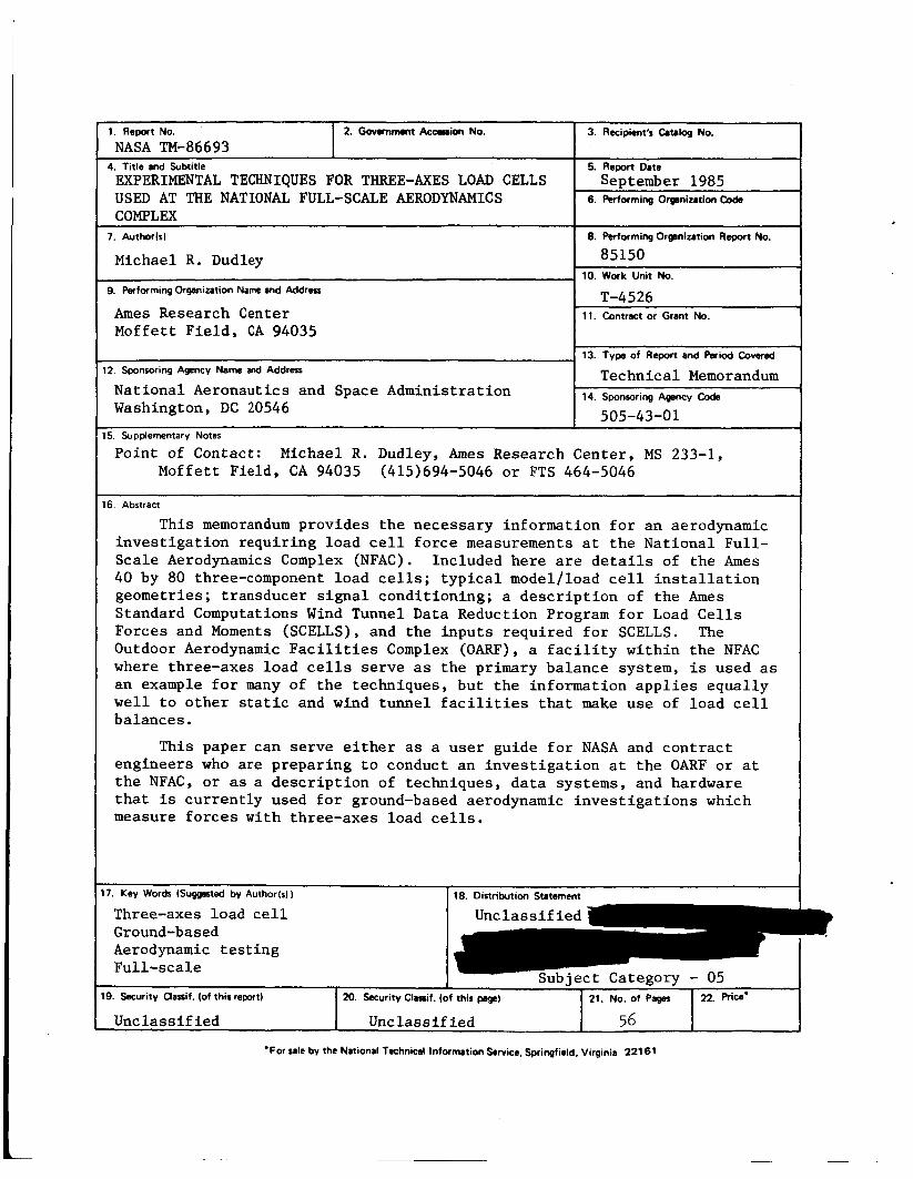
This memorandum provides the necessary information for an aerodynamic investigation requiring load cell force measurements at the National Full- Scale Aerodynamics Complex (NFAC). Included here are details of the Ames 40 by 80 three-component load cells; typical model/load cell installation geometries; transducer signal conditioning; a description of the Ames Standard Computations Wind Tunnel Data Reduction Program for Load Cells Forces and Moments (SCELLS), and the inputs required for SCELLS. The Outdoor Aerodynamic Facilities Complex (OARF), a facility within the NFAC where three-axes load cells serve as the primary balance system, is used as an example for many of the techniques, but the information applies equally well to other static and wind tunnel facilities that make use of load cell balances.
This paper can serve either as a user guide for NASA and contract engineers who are preparing to conduct an investigation at the OARF or at the NFAC, or as a description of techniques, data systems, and hardware that is currently used for ground-based aerodynamic investigations which measure forces with three-axes load cells.
7. Key Words (Suggested by Author(s))
Three-axes load cell Ground-based Aerodynamic testing Full-scale
18. Distribution Statement
Subject Category - 05
Unclassified 1 Unclassified I 56 I *For sale by the National Technical Information Service, Springfield, Virginia 22161