Technical Report Documentation Page

1. Report No.

CA15-2173

2. Government Accession No. 3. Recipient’s Catalog No.

4. Title and Subtitle

Influence of the Spacing of Longitudinal Reinforcement on the Performance of Laterally

5. Report Date

12/21/2015

Loaded CIDH Piles – Analytical Investigation 6. Performing Organization Code

7. Author(s)

Vasileios Papadopoulos and P. Benson Shing

8. Performing Organization Report No.

UCSD/SSRP-15/07

9. Performing Organization Name and Address

Department of Structural Engineering University of California, San Diego

10. Work Unit No. (TRAIS)

9500 Gilman Drive, Mail Code 0085 La Jolla, California 92093-0085

11. Contract or Grant No.

65A0369

12. Sponsoring Agency Name and Address

California Department of Transportation

13. Type of Report and Period Covered

Technical Report

Division of Engineering Services 1801 30th St., MS #9-2/5I Sacramento, California 95816

14. Sponsoring Agency Code

15. Supplementary Notes

Prepared in cooperation with the State of California Department of Transportation. This report on the analytical study is preceded by Report No. UCSD/SSRP-14/08, which documented the experimental investigation conducted in this project.

16. AbstractFor the construction of cast-in-drilled-hole (CIDH) piles in the presence of ground water, slurry is used before and during concrete placement to stabilize the drilled hole. When concrete is placed under slurry, defects may occur, affecting the structural integrity of the pile. In this situation, non-destructive testing, such as gamma-gamma testing, is to be conducted to detect potential anomalies in the concrete. These tests require the placement of inspection (PVC) tubes inside the pile. To accommodate the inspection tubes, the center-to-center spacing of the adjacent longitudinal bars in the pile has to be larger than the 8-in. maximum permitted by the Caltrans Bridge Design Specifications and the AASHTO LRFD Bridge Design Specifications.

This report presents a numerical investigation to study the effect of the spacing of the longitudinal reinforcement in CIDH piles on their structural performance. It is aimed to confirm and generalize the experimental data obtained in this project, which has been reported elsewhere. To this end, three-dimensional nonlinear finite element (FE) models have been developed for RC pile shafts, and used for a numerical parametric study. The modeling method has been validated by experimental data. The parametric study considers piles of different diameters, with different lineal and angular spacings of the longitudinal bars, and with different levels of the axial load. To capture the strength degradation of piles under lateral loading, a phenomenological stress-strain law for steel that accounts for the low-cycle fatigue of bars under large-amplitude cyclic strain reversals has been developed in this study. To model the nonlinear behavior of concrete, a damaged-plasticity model has been used. In addition, a microplane model for concrete has been implemented as an alternative. The latter has been found to be superior in that it does not require artificial remedies to capture the tensile unloading and reloading behavior of concrete and the compressive behavior of confined concrete. The bond-slip behavior between the longitudinal bars and the surrounding concrete is modeled with a phenomenological bond-slip law.

The numerical study has shown that the spacing of the longitudinal bars in circular RC members can be larger than 8 in. without jeopardizing their structural performance. Similar to the experimental findings, the numerical parametric study has shown that the lineal spacing of the longitudinal bars does not have any impact on the ductility of an RC pile. However, the size of the longitudinal bars can affect the ductility of a pile. The load degradation in a pile is often associated with the spalling of the cover concrete, and the buckling and the fracture of the longitude bars in the plastic-hinge region of the pile. Larger-diameter bars are more resistant to buckling for the same spacing of the lateral reinforcement and therefore result in a more ductile behavior. The parametric study has also confirmed that a smaller lineal spacing with smaller-size longitudinal bars can lead to more closely spaced flexural cracks with smaller widths. These observations are true for piles of different diameters and subjected to different levels of axial loads.

17. Key Words

CIDH piles, reinforcement spacing, slurry displacement method, vertical reinforcement, ductility, confinement, crack spacing, crack width, inspection tubes, FEA, constitutive models

18. Distribution Statement

No restrictions. This document is available to the public through the National Technical Information Service, Springfield, Virginia 22161.

19. Security Classification (of this report)

Unclassified

20. Security Classification (of this page)

Unclassified

21. No. of Pages

141

22. Price

Form DOT F 1700.7 (8-72) Reproduction of completed page authorized

STRUCTURAL SYSTEMS

RESEARCH PROJECT

Report No.

SSRP-15/07

Influence of the Spacing of Longitudinal

Reinforcement on the Performance of Laterally

Loaded CIDH Piles – Analytical Investigation

by

Vasileios Papadopoulos

P. Benson Shing

Report Submitted to the California Department of Transportation

under Contract No. 65A0369

December 2015

Department of Structural Engineering

University of California, San Diego

La Jolla, California 92093-0085

University of California, San Diego

Department of Structural Engineering

Structural Systems Research Project

Report No. SSRP-15/07

Influence of the Spacing of Longitudinal Reinforcement on the

Performance of Laterally Loaded CIDH Piles – Analytical

Investigation

by

Vasileios Papadopoulos

Graduate Student Researcher

P. Benson Shing

Professor of Structural Engineering

Final Report Submitted to the California Department of Transportation under

Contract No. 65A0369

Department of Structural Engineering

University of California, San Diego

La Jolla, California 92093-0085

December 2015

i

DISCLAIMER

This document is disseminated in the interest of information exchange. The contents of this report reflect

the views of the authors who are responsible for the facts and accuracy of the data presented herein. The

contents do not necessarily reflect the official views or policies of the State of California or the Federal

Highway Administration. This publication does not constitute a standard, specification or regulation. This

report does not constitute an endorsement by the California Department of Transportation of any product

described herein.

For individuals with sensory disabilities, this document is available in Braille, large print, audiocassette,

or compact disk. To obtain a copy of this document in one of these alternate formats, please contact: the

Division of Research and Innovation, MS-83, California Department of Transportation, P.O. Box 942873,

Sacramento, CA 94273-0001.

ii

TABLE OF CONTENTS

DISCLAIMER ............................................................................................................................................... i

TABLE OF CONTENTS .............................................................................................................................. ii

LIST OF FIGURES ..................................................................................................................................... iv

LIST OF TABLES ....................................................................................................................................... ix

ACKNOWLEDGMENTS ............................................................................................................................ x

ABSTRACT ................................................................................................................................................. xi

CHAPTER 1

........................................................................................................................................ 1 INTRODUCTION

1.1 Background and Motivation of the Study ..................................................................................... 1

1.2 Past Research ................................................................................................................................ 2

1.3 Scope of this Study and Organization of the Report ..................................................................... 3

CHAPTER 2

........................................................................................................................ 7 CONSTITUTIVE MODELS

2.1 Damaged-Plasticity Model for Concrete ....................................................................................... 7

2.1.1 Damaged-Plasticity Model Formulation ............................................................................... 8

2.1.2 Validation and Calibration of the Damaged-Plasticity Model ............................................ 13

2.2 Modeling of Steel Reinforcement ............................................................................................... 15

2.2.1 Cyclic Stress-Strain Relation .............................................................................................. 16

2.2.2 Low-Cycle Fatigue .............................................................................................................. 19

2.2.3 Calibration of Low-cycle Fatigue Law ............................................................................... 20

2.3 Modeling of Bond-Slip ............................................................................................................... 23

2.3.1 Bond-Slip Interface Model .................................................................................................. 23

2.3.2 Bond Stress-Slip Law.......................................................................................................... 24

2.3.3 Normal and Transverse Tangential Stresses ....................................................................... 25

2.3.4 Interface Element Implementation ...................................................................................... 25

CHAPTER 3

FINITE ELEMENT ANALYSES OF PILE SPECIMENS ........................................................................ 46

3.1 Finite Element model .................................................................................................................. 46

3.2 Validation of Finite Element Models with Experimental Results............................................... 48

3.2.1 Load – vs. – Displacement Response .................................................................................. 48

iii

3.2.2 Flexural Crack Spacing ....................................................................................................... 49

3.2.3 Strains in Longitudinal Bars ............................................................................................... 50

3.2.4 Plastic Deformation in the Piles .......................................................................................... 51

3.2.5 Stresses in Concrete ............................................................................................................ 51

3.2.6 Stresses in the Longitudinal Bars ........................................................................................ 52

3.3 Parametric Study with Finite Element Models ........................................................................... 52

3.3.1 Impact of Lineal Spacing of Bars on Ductility ................................................................... 52

3.3.2 Impact of Lineal Spacing of Bars on Flexural Crack Spacing ............................................ 53

3.3.3 Piles with Larger Diameters ................................................................................................ 53

3.3.4 Piles Subjected to Higher Axial Loads ............................................................................... 54

3.3.5 Impact of Inspection Tubes on Nonlinear Behavior of Piles .............................................. 55

3.4 Conclusions ................................................................................................................................. 55

CHAPTER 4

FINITE ELEMENT ANALYSES WITH MICROPLANE MODEL FOR CONCRETE .......................... 81

4.1 Model formulation ...................................................................................................................... 81

4.2 Validation and Calibration of the Microplane model ................................................................. 89

4.3 Finite Element Analysis of pile specimens with the microplane model ..................................... 91

4.3.1 Specimen #1 ........................................................................................................................ 91

4.3.2 Specimen #2 ........................................................................................................................ 93

4.3.3 Flexural Crack Pattern ........................................................................................................ 93

4.4 Summary and Conclusions.......................................................................................................... 94

CHAPTER 5

SUMMARY AND CONCLUSIONS ....................................................................................................... 110

5.1 Summary ................................................................................................................................... 110

5.2 Conclusions ............................................................................................................................... 111

REFERENCES ......................................................................................................................................... 113

iv

LIST OF FIGURES

Figure 1.1 – Typical drilled shaft reinforcement cage with PVC inspection tubes (Caltrans)...................... 5

Figure 1.2 – Effect of spacing of longitudinal bars on circular columns (Mander et al. 1988) .................... 5

Figure 1.3 – Effect of spacing of longitudinal bars on rectangular sections (Mander et al. 1988b) ............. 6

Figure 1.4 – Arching action introduced by confining reinforcement (Mander et al. 1988a) ........................ 6

Figure 2.1 – Stiffness recovery under uniaxial load cycle for damaged-plasticity model .......................... 28

Figure 2.2 – Initial yield function in principal stress space under plane-stress condition (Lee and Fenves

1998) ........................................................................................................................................................... 28

Figure 2.3 – Deviatoric plane for different values of Kc ............................................................................. 29

Figure 2.4 – Meridian plane of yield surface for different values of Kc ..................................................... 29

Figure 2.5 – Plastic potential for different values of .............................................................................. 30

Figure 2.6 – Model for uniaxial loading with contact conditions ............................................................... 30

Figure 2.7 – Uniaxial loading test of models with and without contact conditions .................................... 31

Figure 2.8 – FE model of hydrostatic pressure tests by Hurblut (1985) ..................................................... 31

Figure 2.9 – Confined compression tests by Hurblut (1985) ...................................................................... 32

Figure 2.10 – Calibration of input uniaxial compressive stress-strain curve in damaged-plasticity model

accounting for confinement effect .............................................................................................................. 32

Figure 2.11 – Comparison of model with modified post-peak behavior to experimental results by Hurblut

(1985) .......................................................................................................................................................... 33

Figure 2.12 – FE model of compression tests on confined circular-sectioned RC columns by Mander et al.

(1988b) ........................................................................................................................................................ 33

Figure 2.13 – Comparison of model with modified post-peak behavior to experimental results by Mander

et al. (1988b) ............................................................................................................................................... 34

Figure 2.14 – Steel Model for monotonic loading ...................................................................................... 34

Figure 2.15 –Menegotto-Pinto model for cyclic stress-stain relation ......................................................... 35

Figure 2.16– Hysteretic curves by Menegotto-Pinto model with partial unloading and reloading ............ 35

v

Figure 2.17 – Cyclic tests of steel reinforcing bars by Dodd and Restrepo (1995) .................................... 36

Figure 2.18 – Cyclic tests of steel reinforcing bars by Aktan et al. (1973) ................................................. 37

Figure 2.19 – Cyclic test of steel reinforcing bar by Kent and Park (1973) ............................................... 38

Figure 2.20 – Cycles with constant strain amplitudes................................................................................. 38

Figure 2.21 – Strain ranges, Δε, with random strain reversals .................................................................... 39

Figure 2.22 – Strain reversals with mean strain, mean ............................................................................... 39

Figure 2.23 – Strain reversals with mean stress, mean .............................................................................. 40

Figure 2.24 – Effect of mean strain and stress on LCF (Koh and Stephens, 1991) .................................... 40

Figure 2.25 – LCF test by Kunnath et al. (2009b) ...................................................................................... 41

Figure 2.26 – Integration points in the circular section of a beam element in Abaqus ............................... 41

Figure 2.27 – Cyclic tests of No. 11 bar specimens by Kunnath et al. (2009b) .......................................... 42

Figure 2.28 – Mesh-size sensitivity study with No. 11 bar (Specimen N11Y4) tested by Kunnath et al.

(2009b) ........................................................................................................................................................ 43

Figure 2.29 – Comparison of LCF laws for material level and bar level .................................................... 43

Figure 2.30 – LCF law for No. 9 bars with different slenderness ............................................................... 44

Figure 2.31 – Stresses and relative displacements at the bar-concrete interface ........................................ 44

Figure 2.32 – Analytical bond stress-slip model by Murcia-Delso and Shing (2015) ................................ 45

Figure 2.33 – Interface element by Murcia-Delso and Shing (2015).......................................................... 45

Figure 3.1 – FE model of Specimen #1 ...................................................................................................... 60

Figure 3.2 – Mesh-size sensitivity study with the FE model of Specimen #1 ............................................ 61

Figure 3.3 - Lateral load-vs.- drift ratio curves for Specimen #1 ............................................................... 61

Figure 3.4 – Lateral load-vs.- drift ratio curves for Specimen #2 ............................................................... 62

Figure 3.5 – Numbering of longitudinal bars in Specimens #1 and #2 ....................................................... 62

Figure 3.6 – Flexural cracking in Specimen #1 at 1% drift ........................................................................ 63

Figure 3.7 – Flexural cracking in Specimen #2 at 1% drift ........................................................................ 63

Figure 3.8 – Normal plastic strains in concrete ......................................................................................... 64

vi

Figure 3.9 – Extent of flexural cracking for moment capacities 1pM (Specimen #1) and 2pM (Specimen

#2) ............................................................................................................................................................... 65

Figure 3.10 – Strains along the longitudinal bar 1 at the south face at +4% drift ....................................... 65

Figure 3.11 – Strains in bars at the south face of Specimen #1 at +1% drift .............................................. 66

Figure 3.12 – Strains in bars at the north face of Specimen #1 at -1% drift ............................................... 66

Figure 3.13 – Strains in bars at the south face of Specimen #1 at +4% drift .............................................. 67

Figure 3.14 – Strains in bars at the north face of Specimen #1 at -4% drift ............................................... 67

Figure 3.15 – Strains in bars at the south face of Specimen #1 at +8% drift .............................................. 68

Figure 3.16 – Strains in bars at the north face of Specimen #1 at -8% drift ............................................... 68

Figure 3.17 - Strains in bars at the south face of Specimen #2 at +1% drift ............................................... 69

Figure 3.18 – Strains in bars at north face of Specimen #2 at -1% drift ..................................................... 69

Figure 3.19 – Strains in bars at south face of Specimen #2 at +4% drift .................................................... 70

Figure 3.20 – Strains in bars at north face of Specimen #2 at -4% drift ..................................................... 70

Figure 3.21 – Strains in bars at south face of Specimen #2 at +8% drift .................................................... 71

Figure 3.22 – Strains in bars at north face of Specimen #2 at -8% drift ..................................................... 71

Figure 3.23 – Axial stress-strain curves from cover concrete and core concrete for Specimen #1 ............ 72

Figure 3.24 –Stress-strain curves for longitudinal bars at the base of the pile of Specimen #1 ................. 72

Figure 3.25 – Lateral load-vs.-drift ratio curves for models with D=28 in. ............................................... 73

Figure 3.26 – Cycles at which the longitudinal bars fractured for models with D=28 in. .......................... 73

Figure 3.27 – Normal plastic strains in the axial direction at 1% drift for models with D=28 in. ............. 74

Figure 3.28 – Lateral load-vs.-drift ratio curves for models with D=56 in. ............................................... 75

Figure 3.29 – Normalized lateral load-vs.-drift ratio curves of pile models with different diameter ......... 75

Figure 3.30 – Cycles at which the longitudinal bars fractured for models with D=56 in. .......................... 76

Figure 3.31 – Normal plastic strains in the axial direction at 1% drift for models with D=56 in. ............. 77

Figure 3.32 – Normal plastic strains in the axial direction at 1% drift for piles D28S2 and D56S2 .......... 78

Figure 3.33 – Mesh sensitivity study for the normal plastic strains in pile D56S1 .................................... 78

vii

Figure 3.34 – Lateral load-vs.-drift ratio curves for models with axial load equal to 0.15 c cA f ................ 79

Figure 3.35 – Lateral load-vs.-drift ratio curves for models with axial load equal to 0.20 c cA f ................ 79

Figure 3.36 – FE model of D28S1-B (with PVC inspection tubes) ............................................................ 80

Figure 3.37 – Lateral load-vs.-top drift curve for Specimen D28S1-B (with voids) .................................. 80

Figure 4.1 – (a) System of discrete microplanes, (b) Microplane strain vector and its components (Caner

and Bazant, 2013a) ...................................................................................................................................... 97

Figure 4.2 – Stress-strain boundaries of the microplane model (Caner and Bazant, 2013a) ...................... 97

Figure 4.3 – Vertical return to normal boundary when the boundary is exceeded by an elastic trial stress in

a finite load step (Caner and Bazant, 2013a) .............................................................................................. 98

Figure 4.4 – Comparison of microplane model with default parameters to experimental results by Hurblut

(1985) .......................................................................................................................................................... 98

Figure 4.5 – Comparison of microplane model to uniaxial compression test by van Mier (1986) ............. 99

Figure 4.6 – Comparison of microplane model to experimental results by Mander et al. (1988b) .......... 100

Figure 4.7 – Model for cyclic loading in tension ...................................................................................... 101

Figure 4.8 – Comparison of microplane model and D-P model under cyclic loading in tension ............. 101

Figure 4.9 – FE model of Specimen #1 assembly with microplane model for concrete .......................... 102

Figure 4.10 – Lateral load-vs.-top drift ratio curves for Specimen #1 ...................................................... 103

Figure 4.11 – Deformed shape of FE model of Specimen #1 at 10% drift ............................................... 103

Figure 4.12 – Axial stress-strain curve for cover concrete at the base of Specimen #1 ........................... 104

Figure 4.13 – Axial stress-strain curve for core concrete at the base of Specimen #1 ............................. 104

Figure 4.14 – Cycles at which bars fracture in the FEA of Specimen #1 ................................................. 105

Figure 4.15 – Lateral load-vs.-top drift ratio curves for Specimen #2 ...................................................... 105

Figure 4.16 – Cycles at which bars fracture in the FEA of Specimen #2 ................................................. 105

Figure 4.17 – Strains in bars at south face of Specimen #1 at +1% drift .................................................. 106

Figure 4.18 – Strains in bars at south face of Specimen #1 at +4% drift .................................................. 106

Figure 4.19 – Strains in bars at the south face of Specimen #1 at +8% drift ............................................ 107

Figure 4.20 – Strains in bars at south face of Specimen #2 at +1% drift .................................................. 107

viii

Figure 4.21 – Strains in bars at south face of Specimen #2 at +4% drift .................................................. 108

Figure 4.22 – Strains in bars at south face of Specimen #2 at +8% drift .................................................. 108

Figure 4.23 – Normal strains in concrete at 1% drift ................................................................................ 109

ix

LIST OF TABLES

Table 2.1 – Damaged-plasticity model calibration ..................................................................................... 27

Table 2.2 – Calibration of the Menegotto-Pinto Model .............................................................................. 27

Table 2.3 – Comparison of number of cycles to failure in the FEA and tests ............................................ 27

Table 3.1 – Damaged-plasticity model calibration for concrete in the pile ................................................ 57

Table 3.2 – Steel material parameters for longitudinal reinforcement ........................................................ 57

Table 3.3 – Lateral load capacity of pile specimens ................................................................................... 57

Table 3.4 – Cycles at which bars fractured in Specimen #1 ....................................................................... 58

Table 3.5 – Cycles at which bars fractured in Specimen #2 ....................................................................... 58

Table 3.6 –Piles properties for parametric study ........................................................................................ 58

Table 3.7 – Pile models with varying level of axial load ............................................................................ 59

Table 4.1 – Free parameters of microplane model by Caner and Bazant (2013b) ...................................... 95

Table 4.2 – Fixed parameters of microplane model by Caner and Bazant (2013b) .................................... 95

Table 4.3 – Calibration of microplane model ............................................................................................. 96

Table 4.4 – Cycles at which bars fractured in Specimen #1 ....................................................................... 96

Table 4.5 – Cycles at which bars fractured in Specimen #2 ....................................................................... 96

x

ACKNOWLEDGMENTS

Funding for the investigation presented in this report was provided by the California Department of

Transportation (Caltrans) under Contract No. 65A0369. The authors are most grateful to Caltrans

engineers for their continuous technical input and advice throughout this study. Dr. Charles Sikorsky of

Caltrans was the project manager, who provided unfailing support and guidance, which was instrumental

to the successful completion of this study.

The authors would also like to thank Dr. Juan Murcia Delso for his contributions and advice in the finite

element modeling of RC members, and Dr. Ioannis Koutromanos for his contributions in the

implementation of the microplane model used in this study.

xi

ABSTRACT

For the construction of cast-in-drilled-hole (CIDH) piles in the presence of ground water, slurry is used

before and during concrete placement to stabilize the drilled hole. When concrete is placed under slurry,

defects may occur, affecting the structural integrity of the pile. In this situation, non-destructive testing,

such as gamma-gamma testing, is to be conducted to detect potential anomalies in the concrete. These

tests require the placement of inspection (PVC) tubes inside the pile. To accommodate the inspection

tubes, the center-to-center spacing of the adjacent longitudinal bars in the pile has to be larger than the 8-

in. maximum permitted by the Caltrans Bridge Design Specifications and the AASHTO LRFD Bridge

Design Specifications.

This report presents a numerical investigation to study the effect of the spacing of the longitudinal

reinforcement in CIDH piles on their structural performance. It is aimed to confirm and generalize the

experimental data obtained in this project, which has been reported elsewhere. To this end, three-

dimensional nonlinear finite element (FE) models have been developed for RC pile shafts, and used for a

numerical parametric study. The modeling method has been validated by experimental data. The

parametric study considers piles of different diameters, with different lineal and angular spacings of the

longitudinal bars, and with different levels of the axial load. To capture the strength degradation of piles

under lateral loading, a phenomenological stress-strain law for steel that accounts for the low-cycle

fatigue of bars under large-amplitude cyclic strain reversals has been developed in this study. To model

the nonlinear behavior of concrete, a damaged-plasticity model has been used. In addition, a microplane

model for concrete has been implemented as an alternative. The latter has been found to be superior in

that it does not require artificial remedies to capture the tensile unloading and reloading behavior of

concrete and the compressive behavior of confined concrete. The bond-slip behavior between the

longitudinal bars and the surrounding concrete is modeled with a phenomenological bond-slip law.

xii

The numerical study has shown that the spacing of the longitudinal bars in circular RC members can be

larger than 8 in. without jeopardizing their structural performance. Similar to the experimental findings,

the numerical parametric study has shown that the lineal spacing of the longitudinal bars does not have

any impact on the ductility of an RC pile. However, the size of the longitudinal bars can affect the

ductility of a pile. The load degradation in a pile is often associated with the spalling of the cover

concrete, and the buckling and the fracture of the longitude bars in the plastic-hinge region of the pile.

Larger-diameter bars are more resistant to buckling for the same spacing of the lateral reinforcement and

therefore result in a more ductile behavior. The parametric study has also confirmed that a smaller lineal

spacing with smaller-size longitudinal bars can lead to more closely spaced flexural cracks with smaller

widths. These observations are true for piles of different diameters and subjected to different levels of

axial loads.

1

CHAPTER 1

INTRODUCTION

1.1 Background and Motivation of the Study

For the construction of cast-in-drilled-hole (CIDH) piles in the presence of ground water, slurry is used

before and during concrete placement to stabilize the drilled hole. When concrete is placed under slurry,

defects may occur, affecting the structural integrity of the pile. Hence, the construction of CIDH piles

larger than 2 ft. in diameter under wet conditions requires the installation of inspection (PVC) tubes for

non-destructive detection of potential anomalies in the concrete, as shown in Figure 1.1. Normally, one

inspection tube is required per foot of pile diameter. The inspection tubes are placed around the pile

reinforcement cage in contact with the inside of the outer most hoop reinforcement and must be at least

three (3) inches clear of the vertical reinforcement, as shown in Figure 1.1. This will require that the clear

spacing between the longitudinal reinforcing bars in the reinforcement cage immediately adjacent to a

tube be at least 8.5 in. so that the clear spacing between a tube and an adjacent bar will be at least 3 in. to

allow a good flow of concrete. For Type I shafts, the spacing of longitudinal bars in both the column and

the shaft is the same. Hence, the placement of inspection tubes will necessitate the violation of the

maximum allowable center-to-center spacing of 8 in. for longitudinal bars, as specified in both the

Caltrans Bridge Design Specifications (2004) and the AASHTO LRFD Bridge Design Specifications

(2014).

Because of the lack of research data on the influence of the spacing of longitudinal reinforcement on the

structural performance of reinforced concrete piles and circular columns, a research program was carried

out to investigate this influence, especially the impact of a spacing exceeding the current Caltrans and

AASHTO limits of 8 in. The research consisted of both experimental and numerical investigations.

2

Results and findings of the experimental investigation can be found in Papadopoulos and Shing (2014).

This report presents details of the nonlinear finite element models used in the numerical investigation, the

model calibration, and the findings of a numerical parametric study extrapolating the experimental results.

1.2 Past Research

The influence of the quantity and spacing of transverse reinforcement on the ductility and structural

performance of RC members subjected to axial loads and flexure has been well studied and understood.

However, there is only limited information on the influence of the spacing of longitudinal reinforcement

on the structural performance of RC members. It has been perceived that a larger spacing could

negatively affect the efficiency of confinement on concrete and, thereby, reduce the flexural ductility of

the member (Pauley and Priestley 1992). While this can be understood for members with rectangular

sections, in which the spacing of the cross-ties is normally related to the spacing of the longitudinal bars,

it is less so for circular members. Both Caltrans (2004) and AASHTO (2014) have specified a spacing

limit of 8 in. for compression members regardless of the cross-sectional shape. Nevertheless, from the

structural performance standpoint, the spacing limit for the longitudinal bars in a circular member should

depend on the diameter of the member, and it is reasonable to expect that a member with a larger diameter

can have a larger circumferential spacing of the longitudinal bars without affecting its structural

performance. Limited experimental data obtained by Mander et al. (1988b) have shown that the influence

of the spacing of longitudinal bars on the behavior of circular RC columns under compression is almost

negligible, as shown in Figure 1.2. However, the maximum center-to-center spacing of longitudinal bars

considered in their study was less than 6.5 in. Furthermore, there is no data on the influence of the bar

spacing on the behavior of a circular member under simultaneous axial load and flexure. For rectangular

columns, a closer spacing of longitudinal bars has a clear benefit of enhancing the compressive strength

and ductility of the member, as shown in Figure 1.3. This is because a closer spacing of longitudinal bars

3

in rectangular columns requires a closer spacing of cross-ties, which results in a better arching action and

a more effectively confined core as shown in Figure 1.4.

To investigate the impact of the spacing of longitudinal bars on the performance of a circular-sectioned

member subjected to simultaneous axial and fully reversed cyclic lateral loading, two pile specimens were

tested in the Powell Structural Engineering Laboratory of the University of California at San Diego. The

two specimens had the same dimensions. One specimen was designed according to the Caltrans Bridge

Design Specifications (2004) and the AASHTO LRFD Bridge Design Specifications (2014). The other

had the same design except that its longitudinal reinforcement had spacing greater than 8 in., violating

current design requirements. The test results show that the spacing of the longitudinal bars had no

influence on the ductility of the pile specimens. Details of the experimental study and findings have been

documented in a separate report (Papadopoulos and Shing 2014).

1.3 Scope of this Study and Organization of the Report

The experimental study reported by Papadopoulos and Shing (2014) provided only one comparison of

two pile specimens with the longitudinal bar spacing and bar size being the only variables. To have more

data to confirm the experimental observation, numerical parametric studies using detailed nonlinear finite

element models have been carried out, considering piles of different diameters and varying the lineal as

well as the angular spacing of the longitudinal bars and the level of the axial load. The nonlinear finite

element modeling methods used in the study have been first validated with the aforementioned

experimental results. The finite element analyses have been performed with the commercial program

Abaqus (Simulia 2012). This report documents the numerical study, including the constitutive models

used and their calibration, the finite element models developed for the pile analyses, and the findings of

the numerical parametric study. It has the following organization.

4

Chapter 2 of this report presents the constitutive models used to describe the behavior of concrete and

reinforcing steel under cyclic stress reversals. A damaged-plasticity model provided in Abaqus (Lubliner

et al., 1989, Lee and Fenves, 1998) is used to model concrete. It has been validated and calibrated with

uniaxial and tri-axial test data from other studies. A phenomenological steel model developed in this

study to account for the low-cycle fatigue of reinforcing bars under large cyclic strain reversals is

thoroughly presented. A method to account for the large localized strains induced by the buckling of a bar

is also described. Finally, this chapter presents the phenomenological bond-slip law, proposed by Murcia-

Delso and Shing (2015), which is used to model bond slip between longitudinal bars and the surrounding

concrete in the FE analyses.

Chapter 3 describes the finite element models developed to simulate the behavior of the two RC pile

specimens tested in the laboratory as reported by Papadopoulos and Shing (2014). The finite element

models have been validated with the test results. With this finite element modeling method, a parametric

study, considering piles of different diameters and varying the lineal spacing of the longitudinal bars and

the level of the axial load, is presented.

Chapter 4 presents the microplane model by Caner and Bazant (2013a), an alternative constitutive model

for concrete which has been implemented in Abaqus to overcome the deficiencies of the damaged-

plasticity model. The microplane model has been used in the finite element models of the pile specimens

tested in this study. The results of the finite element analyses are compared to the test data of the pile

specimens. Finally, a summary and the conclusions of this study are provided in Chapter 5.

5

Figure 1.1 – Typical drilled shaft reinforcement cage with PVC inspection tubes (Caltrans)

Figure 1.2 – Effect of spacing of longitudinal bars on circular columns (Mander et al. 1988)

0

10

20

30

40

50

60

0.00 0.01 0.02 0.03 0.04 0.05 0.06 0.07

Stre

ss o

f co

re (

MP

a)

strain

column 7

column 9

column 12

12 @ 52

0.02s

D mm

Column 12 24 D16 bars ρl = 0.0246 s = 2.05’’

Column 9 16 D20 bars ρl = 0.0256 s = 3.08’’

Column 7 8 D28 bars ρl = 0.0251 s = 6.15’’

6

Figure 1.3 – Effect of spacing of longitudinal bars on rectangular sections (Mander et al. 1988b)

Figure 1.4 – Arching action introduced by confining reinforcement (Mander et al. 1988a)

0

10

20

30

40

50

60

70

80

90

0.00 0.01 0.02 0.03 0.04 0.05 0.06

Stre

ss o

f co

re (

MP

a)

strain

wall 12

wall 13

wall 12 wall 13

(a) Rectangular column (b) Circular column

0.0108 (10 D12)

3.6 '' (spacing)

0.0786 (R10 @ 42mm)

l

s

s

0.0306 (16 D16 )

6.3'' (spacing)

0.0708 (R10@30mm)

l

s

s

7

CHAPTER 2

CONSTITUTIVE MODELS

The commercial program Abaqus (Simulia, 2012) has been used for the pile analyses conducted in this

study. This chapter presents the constitutive models used to describe the nonlinear behaviors of concrete

and reinforcing steel, and the bond-slip behavior between a reinforcing bar and the surrounding concrete

in the analyses. Concrete is modeled as a continuum using the 3-D damaged-plasticity constitutive law

that is available in Abaqus. Longitudinal reinforcement is modeled with beam elements using a

phenomenological stress-strain law developed in this study to account for the low-cycle fatigue of bars

under large-amplitude cyclic strain reversals. The finite element models also account for the slip of the

longitudinal reinforcing bars in concrete, which has a profound influence on the plastic strain localization

and subsequent fracture of bars. This behavior is simulated with a bond-slip law developed by Murcia-

Delso and Shing (2015).

2.1 Damaged-Plasticity Model for Concrete

Models combining plasticity and damage mechanics theories are attractive for simulating the behavior of

concrete in that they can account for both plastic deformation and stiffness degradation in concrete under

severe multi-axial stress reversals. The concrete damaged-plasticity model available in Abaqus is based

on the formulations proposed by Lubliner et al. (1989) and Lee and Fenves (1998). This section

summarizes the basic formulation for this model, and describes how the model has been calibrated and

validated in this study with the experimental data of Hurblut (1985) and Mander et al. (1988b).

8

2.1.1 Damaged-Plasticity Model Formulation

The model complies with the classical theory of plasticity in that the strain tensor is decomposed into an

elastic part and a plastic part, and the stress tensor is obtained as the double contraction of the elastic

stiffness tensor and the elastic strain tensor.

e pε = ε +ε (2.1)

: :e pσ = Ε ε = E ε -ε (2.2)

To account for stiffness degradation using the damage mechanics theory, the elastic stiffness tensor is

related to the initial stiffness tensor as:

(1 )d oE E (2.3)

where d is a scalar damage parameter that assumes a value between 0 and 1, with 0 representing the state

of no damage. For a uniaxial stress state, d can be interpreted as the ratio of the damaged cross-sectional

area, which cannot carry any load, to the total cross-sectional area under consideration. The actual stress

developed in the undamaged material is called the effective stress and is defined as:

: :e p

o oσ = Ε ε = Ε ε -ε (2.4)

The damage parameter d is a function of the damage parameter in tension, p

t td , and the damage

parameter in compression, p

c cd , as follows:

(1 ) 1 1t c c td s d s d (2.5)

9

The damage parameters, p

t t td d and p

c c cd d , are calibrated from cyclic uniaxial tension and

compression tests and are functions of the plastic tensile and compressive strain, respectively.

Variables ts and cs are defined as:

ˆ1t ts w r σ (2.6)

ˆ1 1c cs w r σ (2.7)

In Eq. (2.6) and (2.7), tw and cw are constants that control the recovery of stiffness upon stress reversal

from compression to tension and from tension to compression, respectively. The values of tw and cw can

be between 0, where no stiffness recovery is assigned, and 1, where total stiffness recovery is assigned.

ˆr σ is a weight factor, with a value between 0 and 1, defined as:

3

1

3

1

ˆ0 if

ˆˆ ˆ ; 0 1

otherwiseˆ

i

i

i

i

r r

σ 0

σ σ (2.8)

where ˆi ’s are the principal effective stresses.

The solid line in Figure 2.1 shows the stress-strain response of the concrete model under uniaxial loading,

with total stiffness recovery ( 1cw ) upon stress reversal from tension to compression, and no stiffness

recovery ( 0tw ) from compression to tension.

10

The equivalent plastic strains, p

c and p

t , are calculated from the equivalent plastic strain rates, p

c

and p

t , as follows:

0

t

p p

t t dt (2.9)

0

t

p p

c c dt (2.10)

The equivalent plastic strain rates, p

c and p

t , are evaluated with the following expressions:

maxˆˆp p

t r σ (2.11)

minˆˆ1p p

c r σ (2.12)

in which maxˆ p and

minˆ p are obtained from the principal plastic strain rates ( 1 2 3, ,p p p ) in that

max 1ˆ p p

and min 3ˆ p p with 1 2 3

p p p .

The yield surface of the damaged-plasticity model is based on that proposed by Lubliner et al. (1989) with

the modifications introduced by Lee and Fenves (1998) to account for the different behaviors of concrete

in tension and compression. The initial shape of the yield surface in the principal stress plane for the

plane-stress condition is shown in Figure 2.2. The yield function is defined in terms of the first stress

invariant 1I , the second deviatoric stress invariant 2J , and the maximum principal stress as max̂ :

1 2 max max

1ˆ ˆ3 ,

1

p p p

c t c cF aI Ja

(2.13)

11

in which < - > denotes the Macauley brackets. Variable c , along with t , which is used to calculate

variable , defined in Eq. (2.19), are the effective compressive and tensile cohesion strengths, and are

defined as:

1

cc

cd

(2.14)

1

tt

td

(2.15)

in which the functions p

t t and p

c c represent the stress-vs.-plastic strain curves for uniaxial

tension and compression, and are calibrated from uniaxial tension and compression test data.

Constant a in Eq. (2.13) is defined as:

0 0

0 0

/ 1

2 / 1

b c

b c

a

(2.16)

in which 0 0/b c is the ratio of the initial equibiaxial compressive yield stress to the initial uniaxial

compressive yield stress. In this study, the default value of 1.16 is used for 0 0/b c . Constant is

defined as:

3 1

2 1

c

c

K

K

(2.17)

in which cK , as defined in Eq. (2.18), is the ratio of the second deviatoric stress invariant for a stress

state on the tensile meridian to that on the compressive meridian at the initial yield, for any given value of

the pressure invariant such that the maximum principal stress is negative, maxˆ 0 .

12

2

2

TMc

CM

JK

J (2.18)

The value of cK must satisfy the condition that 0.5 1.0cK . As shown in Figure 2.3, the shape of the

deviatoric plane depends on the value of cK . The value of cK also affects the slopes of the tensile and

compressive meridians in the meridian plane as it is shown in Figure 2.4. For low hydrostatic pressure

states, 2 / 3cK provides a good fit of experimental data, while a higher value of cK is more

appropriate for high hydrostatic pressure states, as pointed out by Ottosen (1977).

The variable is defined as:

1 1

p

c c

p

t t

a a

(2.19)

For the yield surface originally proposed by Lubliner et al. (1989), is a constant, dependent only on

the initial ratio of /c t . According to Lee and Fenves (1998), this gives good results for monotonic

loading, but to model the cyclic behavior of concrete, has to be dependent on the evolution of the

compressive strength and tensile strength.

A non-associated flow rule has been adopted with the plastic strain rate is defined as G

pε

σ, where

is the plastic multiplier. The plastic potential G is defined as:

2 1

0 2tan 3 tan3

t

IG J (2.20)

where 0t is the uniaxial tensile strength, which can be obtained from uniaxial tension test data, is the

dilation angle and is a parameter, referred to as the eccentricity that defines the rate at which the

13

function approaches the asymptote. Figure 2.5 shows the shape of the plastic potential for different values

of . The plastic potential tends to a straight line as approaches zero as shown in the figure. For 0 ,

the plastic potential takes the form of the Drucker-Prager (1952) criterion. The default value for is 0.1.

2.1.2 Validation and Calibration of the Damaged-Plasticity Model

Lee and Fenves (1998) validated the model for monotonic uniaxial and biaxial compression and tension

loading. The model available in Abaqus (Simulia 2012) has been calibrated and further validated here for

cyclic uniaxial compression-tension behavior and compression under lateral confinement. The calibration

of the model in Abaqus requires the specification of the uniaxial compressive stress- inelastic strain curve

and the uniaxial tensile stress-cracking displacement curve. Given the value of the compressive strength

of concrete, the uniaxial compressive stress-plastic strain curve has been defined in this study based on

the model proposed by Karthik and Mander (2011) for unconfined concrete. For tension, the tensile

strength is assumed to decay linearly with the cracking displacement, reflecting the fracture energy

released.

In cyclic loading, the damaged-plasticity model has stiffness degradation during unloading and reloading

in tension to simulate the closing and opening of a crack. However, when the inelastic tensile strain is

large, the complete closure of a crack would require a very large stiffness degradation (with the value of

the damage parameter, td , very close to one), which leads to numerical problems. Hence, the model

cannot be appropriately calibrated to simulate the complete closure of a crack with a small residual crack

opening upon unloading. To circumvent this problem, contact conditions in Abaqus are used in this study

to represent major flexural cracks in a discrete manner. Figure 2.6 shows a simple assembly of a finite

element (FE) model which demonstrates how contact conditions can improve the behavior of concrete in

simulation under uniaxial cyclic loading. In Figure 2.7, the dashed curve is the result from the model

without contact conditions, and the solid curve is the result when contact conditions are introduced as

shown in Figure 2.6.

14

The parameters affecting the yield surface have been calibrated with experimental data obtained by

Hurblut (1985) and Mander et al. (1988b) to capture the behavior of confined concrete in compression.

The values of the parameters determined for the damaged-plasticity model are shown in Table 2.1.

Figure 2.8 shows a FE model to simulate the compressive behavior of concrete under equal bilateral

compressive stresses. The assembly, whose mesh has 100 elements is simply supported at its base, and

hydrostatic pressure is applied first. Then, additional compression is applied in one direction by

controlling the displacement of the top face. As shown in Figure 2.9, the model is capable of reproducing

the effect of the lateral confining stress on the compressive strength and lateral expansion of concrete

observed in the tests of Hurblut (1985). However, the increase of ductility in compression (i.e., a less

steep declining slope in the stress-strain curve) due to increasing confining pressure is not captured by the

model. This is due to the fact that the softening rule used in this damaged-plasticity model is defined only

in terms of the uniaxial compressive stress-strain curve, which is embedded in the term p

c cc , as

shown in the expression for the yield surface in Eq. (2.13), without taking into account the effect of the

confining pressure. For the model to match the experimental results, the slope of the decaying branch of

the input uniaxial compressive stress-strain curve has to be modified a priori based on the level of the

confining pressure or the amount of the confining steel, as shown in Figure 2.10. In this figure, cf is the

uniaxial compressive strength of unconfined concrete, while ccf is the uniaxial compressive strength of

confined concrete. In this study, the post-peak slope of the input uniaxial compressive stress-strain curve

is determined according to the confinement level based on the work of Karthik and Mander (2011). With

this modification, the model is capable of capturing the increase of ductility with the increase of the

confining pressure, which was observed in the tests of Hurblut (1985) as shown in Figure 2.11.

The damaged-plasticity model was further validated by replicating the experimental results of Mander et

al. (1988b) on the compression tests of circular-sectioned RC columns with different amounts of

confining steel. Figure 2.12 shows a FE model of one of the RC columns tested by Mander et al. (1988b).

15

The longitudinal bars are modeled with beam elements and the hoops are modeled with truss elements.

An elasto-plastic constitutive law with linear kinematic hardening is assigned to the steel reinforcement.

As shown in Figure 2.13, the FE model can adequately describe the effect of the lateral confining stress

on the compressive strength and ductility of the RC columns, as shown in the experimental tests of

Mander et al. (1988b).

2.2 Modeling of Steel Reinforcement

For the purpose of this study, the stress-strain relation for steel reinforcing bars under cyclic loading has

to be accurately described and efficient to calculate. However, Abaqus (Simulia 2012) only provides an

elasto-plastic constitutive law with linear kinematic hardening. For this reason, a more realistic uniaxial

stress-strain model has been implemented in Abaqus. In this model, the stress-strain relation for cyclic

loading is based on the Menegotto-Pinto model (1973), and the low-cycle fatigue (LCF) law proposed by

Manson (1953) and Coffin (1954) is incorporated. This steel model has been used in beam and truss

elements.

A number of phenomenological steel models have been proposed in various studies to simulate the

behavior of steel reinforcement under cyclic loading. Filippou et al. (1983) have adopted the Menegotto-

Pinto model (1973), and added isotropic hardening to it. Dodd and Restrepo (1995) have proposed an

analytical model that differentiates tensile behavior from compressive behavior by formulating the basic

stress-strain relation in terms of the natural strain and true stress, and then converting it to a relation in

terms of the engineering stress and strain based on an assumption that the volume of the reinforcing bar

remains constant. Monti and Nutti (1992) have proposed a phenomenological stress-strain law that

indirectly accounts for the drop of compressive resistance due to bar buckling. Kunnath et al. (2009a)

have proposed a phenomenological steel model accounting for the LCF of a reinforcing bar based on the

law developed by Manson (1953) and Coffin (1954). The model has been calibrated with experimental

16

data from LCF tests of bar specimens with specific slenderness ratios and a range of bar diameters. For

the basic uniaxial stress-strain relation, Kunnath et al. (2009a) have adopted the Menegotto-Pinto model

(1973) with modifications. They have also adopted the work of Dhakal and Maekawa (2002) to describe

the drop of compressive strength due to bar buckling in the material model.

In this study, the Menegotto-Pinto model (1973) has been adopted, due to its simple formulation, and

improved to better capture the stress-strain behavior of reinforcing bars when they are subjected to partial

unloading and reloading, for which the original formulation has an issue. Similar to Kunnath et al.’s

model (2009a), the LCF law proposed by Manson (1953) and Coffin (1954) has been incorporated. This

law has been calibrated with experimental data obtained from LCF tests conducted on reinforcing bars.

To account for bar buckling occurring in these tests, a calibration method is proposed here to extract the

LCF properties of steel at the material level.

2.2.1 Cyclic Stress-Strain Relation

The model adopted here is formulated in terms of the engineering stress and strain. For a reinforcing bar

made of mild steel and subjected to monotonically increasing strain, the model represents the stress-strain

relation in tension or compression with four segments: (a) a linearly elastic segment, (b) a plateau at the

yield stress, yf , (c) a strain hardening segment described by the Menegotto-Pinto relation, and (d) a

plateau at the ultimate stress, uf . As shown in Figure 2.14, the aforementioned idealized stress-strain

relation matches the tensile test result for a No. 11 well. The ultimate strain at which bar fracture occurs is

determined by a LCF law, which will be described later.

Upon strain reversal after the yield strain, y , has been reached in tension or compression, the

Menegotto-Pinto model (1973) is used to describe the cyclic stress-strain relation, as shown in Figure

2.15. The Menegotto-Pinto model (1973) has the following formulation:

17

** *

1*

(1 )

1 R R

bb

(2.21)

where

* r

o r

(2.22)

* r

o r

(2.23)

Eq. (2.21) relates the normalized stress, * , to the normalized strain,

* , representing the stress-strain

curve for unloading from the strain reversal point ,r r and reloading in the other direction. This curve

has two asymptotes. One has a slope corresponding to the modulus of elasticity of steel and the other has

a slope governing kinematic hardening. Figure 2.15 shows the stress-strain relation without

normalization. In this figure, o and o are the stress and strain at which the two asymptotes meet. The

second asymptote intersects with the straight line representing the linearly elastic behavior of steel under

monotonic loading at , ,,y m y mf or , ,,y m y mf depending on whether it is on the tension or the

compression side. Parameters ,y m and ,y mf assume positive values that are determined by calibration.

Parameter b in Eq. (2.21) governs kinematic hardening in that 1 0/b E E , where 0E is the modulus of

elasticity and 1E is the slope of the second asymptote, as shown in Figure 2.15, and R is a parameter

which controls the stress-strain curvature of the curve simulating the Bauschinger effect. A smaller value

of R corresponds to a larger radius of curvature. The values of ,o o , and ,r r are updated after

each strain reversal. In the original Menegotto-Pinto model, R is calculated with the following equation:

18

10

2

aR R

a

(2.24)

where the variable is defined as:

max

,

min

,

for reloading from compression to tension

for reloading from tension to compression

o

y m

o

y m

(2.25)

in which max and min are the maximum and minimum strains attained in previous cycles. The

constants, 0 1 2, , and R a a , are determined by calibration.

One issue with the original Menegotto-Pinto model is that it is not able to accurately reproduce the stress-

strain response during reloading right after partial unloading, showing stress overshoot, as noted by

Filippou et al. (1983) and Kunnath et al. (2009a). This is illustrated in Figure 2.16, in which the curve

with the original R, calculated with Eq. (2.24), shows a significant stress overshoot during reloading on

the compression side. Besides the inaccuracy, this can also cause convergence problems in finite element

analysis. In this study, this problem is corrected by introducing a modification to the expression for R in

Eq. (2.24) so that the value of R also depends on the stress difference between the intersection point of

the asymptotes, ,o o , and the previous load reversal point, ,r r , as shown in the following

equation.

12

1

2 ,2

o

o ro

y m

aR R

a f

(2.26)

in which is the stress at the previous step. The curve with the modified R in Figure 2.16 shows that

this change corrects the stress overshoot problem.

19

The steel model has been validated with experimental data. Figure 2.17 through Figure 2.19 compare

stress-strain curves from the steel model and the tests conducted by Dodd and Restrepo (1995), Aktan et

al. (1973), and Kent and Park (2973). The values of the model parameters used in the analyses are

summarized in Table 2.2.

2.2.2 Low-Cycle Fatigue

Under severe earthquake loading, flexural reinforcement in plastic-hinge regions of RC members can be

subjected to large-amplitude cyclic plastic strain reversals, due to direct tension or bending once the

reinforcing bars have buckled. Hence, bar fracture is highly influenced by low-cycle fatigue (LCF).

The LCF of steel under cyclic loading with constant strain amplitude can be described with the following

expression by Manson (1953) and Coffin (1954), as adopted in this study:

1

2

c

f

f

N

(2.27)

in which fN is the number of half cycles to failure and is the strain range, defined as

max min , attained in the cyclic loading, as shown in Figure 2.20; and f and c are coefficients

representing the LCF properties of the material. Parameters f and c have to be calibrated with

experimental data.

To account for the random strain history during an earthquake event, the range counting method is

adopted, and damage due to LCF is linearly accumulated according to Miner’s rule (1945). During any

strain reversal i , the strain range max, min,i i i is computed in terms of the maximum and minimum

strains attained in that half cycle no matter it is completed or not, as shown in Figure 2.21, and damage in

that half cycle is defined as:

20

1i

f i

DN

(2.28)

in which f iN is the number of half cycles to failure if the strain range were constant at i according

to Eq. (2.27). Total damage due to LCF during or right after the completion of the nth half cycle is then

calculated as follows:

1

n

i

i

D D

(2.29)

When the damage accumulated reaches or exceeds one, it is assumed that the steel will fracture and the

stress will drop to zero following a steep descending curve in the stress-strain relation. However, in order

to ensure the robustness of the finite element analyses (FEA), fracture is not sudden and the stress drop

follows a descending curve that has a slope equal to 00.034E till it reaches a residual stress of 0.1 yf .

The effects of the mean strain, mean , and mean stress, mean , which are defined in Figure 2.22 and Figure

2.23, are not taken into consideration in the LCF law adopted here. The strain amplitudes, defined as

/ 2 , of interest in this study are above 0.01. According to Koh and Stephens (1991), the effects of the

mean strain and mean stress on the LCF of steel can be neglected for strain amplitudes above that level, as

shown in Figure 2.24.

2.2.3 Calibration of Low-cycle Fatigue Law

In LCF tests, reinforcing bars were normally subjected to severe tensile and compressive load cycles, and

would eventually buckle. Bar buckling exacerbated LCF because of large localized strains introduced by

bar bending. In RC columns, flexural reinforcement in the plastic-hinge region may buckle after the cover

concrete spalls, accelerating the LCF of these bars. The tendency of a bar to buckle depends on its

slenderness ratio, which depends on the bar diameter and its unsupported length as determined by the

21

spacing of the lateral reinforcement in the RC member. Therefore, LCF laws directly calibrated with tests

conducted on bars with specific slenderness ratios may not reflect the true material behavior and

introduce an issue in modeling. If the computational model explicitly captures bar buckling, the model so

calibrated will double count the effect of bar buckling on LCF. If the model does not explicitly consider

bar buckling, then the calibrated model, in the strict sense, will only be appropriate for bars that have a

similar slenderness ratio as the specimens that provided the data. To address this issue, a calibration

strategy is proposed here.

The proposed strategy uses a nonlinear beam element model that captures bar buckling to extract the LCF

properties of the steel material from the LCF tests of the bars. The bar is modeled with beam elements in

Abaqus considering material and geometric nonlinearities. For material nonlinearity, the Menegotto-Pinto

model with the LCF law of Manson and Coffin [Eq. (2.28)] as presented in the previous sections is used.

To calibrate the material model, the LCF tests conducted by Brown and Kunnath (2004) and Kunnath et

al. (2009b) are considered. Figure 2.25a shows the test apparatus used by Kunnath et al. (2009b)

including a buckled bar specimen, while Figure 2.25b shows the FE model for the bar specimen. The bar

is modeled with 2-node beam elements with one integration point at their middle length. The bending

moment and axial force at the sampled section of a beam element are calculated with the trapezoidal rule

based on stresses determined at the cross-sectional sampling points shown in Figure 2.26. The axial

strains of the bars reported for these tests are the average values based on the axial deformation measured

over the entire unsupported length of the bar specimen. The bar is modeled with 10 beam elements with

an initial imperfection (initial offset at mid-span) of /1000L . The FE model is subjected to the same

average-axial strain history (or more exactly the relative end displacement) experienced by the bar during

the test. The values of f and c for the LCF law are so determined that the model exhibits bar fracture in

the same cycle as in the test of the bar specimen. The stress-average axial strain curves obtained by the FE

model and the tests by Kunnath et al. (2009b) are compared in Figure 2.27. The decrease of the

compressive resistance due to the buckling of the bars is adequately described by the FE model. The

22

element size has been determined with a mesh sensitivity analysis. Figure 2.28 shows the stress-strain

curves for FE models with different element sizes.

The LCF law has been calibrated with tests conducted on No. 9, 11, and 14 bars obtained by Brown and

Kunnath (2004) and Kunnath et al. (2009b). The values of f and c have been determined to be 0.382

and 0.455, respectively. Table 2.3 compares the number of cycles to failure, / 2fN , obtained by the FE

analyses with this calibration and the tests. Figure 2.29 compares the LCF law calibrated here for the steel

material to the LCF law calibrated by Brown and Kunnath (2004) directly with the average strain data for

a No. 9 bar that had clear length of 6 times the bar diameter. As expected, the LCF law calibrated for the

material gives a much larger number of cycles to failure for a given strain amplitude.

The use of nonlinear beam elements to model the buckling and LCF of reinforcing bars in RC members

requires very refined FE meshes, at least for the plastic-hinge regions, and thus significant computational

resources. Very often, geometric nonlinearity is ignored in the modeling of reinforcing bars and a mesh

that is coarser than what is needed to simulate bar buckling is used to improve computational efficiency.

It is even more common to represent reinforcing bars with truss elements, which only simulate the

uniaxial stress-strain behavior of bars. With these simplified models, the LCF law calibrated for steel

material will not be appropriate because the effect of bar buckling is not accounted for. On the other hand,

a LCF law calibrated directly with bar test data may not be appropriate for bars that have a slenderness

ratio different from that of the bar specimen that provided the data. The slenderness ratio will affect the

tendency of the bar to buckle and the resulting bending deformation. In an RC member, the slenderness of

a longitudinal reinforcing bar after the cover concrete spalls is governed by the spacing of the lateral

reinforcement.

To address the aforementioned issue, the following procedure is used to calibrate the steel model when

bar buckling is not explicitly accounted for in the FE analysis of an RC member or structure. First, a

single bar is modeled with a refined mesh using nonlinear beam elements which account for bar buckling.

23

The LCF law calibrated for the steel material is used. The clear length of the bar is set to be equal to the

center-to-center spacing of the lateral reinforcement in the member. Finite element analyses are conducted

with the model to simulate LCF tests with varying average-strain ranges. For each strain range, , the

number of cycles to fracture is obtained. A plot of fN versus is then generated with the numerical

data. From this plot, the values of f and c are determined to obtain a LCF law that accounts for the

effect of bar buckling and can therefore be used for simplified bar models used in the structural analysis.

This has to be repeated for every bar size and every lateral steel spacing. Figure 2.30 shows results

obtained for No. 9 bars with different slenderness.

2.3 Modeling of Bond-Slip

The bond-slip behavior between the longitudinal bars and the concrete in an RC member is simulated in

the finite element analyses (FEA) with a bond-slip model developed by Murcia-Delso and Shing (2015).

The model adopts a semi-empirical law, based on concepts originally proposed by Eligehausen et al.

(1983) and further extended by others (Pochanart and Harmon 1989; Yankelevsky et al. 1992 and Lowes

et al. 2004), accounting for bond deterioration caused by cyclic slip reversals, the tensile yielding of the

bars, and the opening of radial splitting cracks in concrete. The bond-slip model has been implemented in

interface elements in Abaqus, which can be used to connect steel to concrete in the three-dimensional

FEA of RC members.

2.3.1 Bond-Slip Interface Model

The relative displacements and stresses in the normal and tangential directions of the interface between a

reinforcing bar and the surrounding concrete are defined in Figure 2.31. The bar slip and bond stress are

denoted by s2 and τ2, respectively.

24

2.3.2 Bond Stress-Slip Law

In the bond-slip law of Murcia-Delso and Shing (2015), the total bond resistance consists of the bearing

resistance and the friction resistance. Figure 2.32(a) shows the monotonic bond stress-slip curves with the

contributions of these two mechanisms. The model has three parameters, namely, the peak bond strength

for an elastic bar, max , the slip at which the peak strength is attained, peaks , and the clear spacing

between the ribs, Rs , to calibrate. Rs is a known geometric property of the bar and is usually between

40% and 60% of the bar diameter. max and peaks depend on many factors and no theoretical formulas are

available to accurately predict their values. Thus, they should be determined experimentally for each case,

if possible. When no experimental data are available, the following empirical formulas can be used to

estimate the values as suggested by Murcia-Delso and Shing (2015).

3/4

max 0.72 (in ksi)cf (2.30)

0.07peak bs d (2.31)

in which cf is the compressive strength of concrete and bd is the bar diameter.

The bond-slip model accounts for the deterioration of both the bearing and the fiction resistances as a

function of the maximum and cumulative slips, the yielding of the bar in tension, and the opening of the

steel-concrete interface with respect to the rib height. Figure 2.32(b) shows the bond stress-vs.-slip

relations for cyclic loading. As shown in the figure, when the bar slips between previously attained slip

levels, the bond stress is bounded by the friction resistance, rev . This is because part of the concrete in

contact with the ribs of the bar on the bearing side has been crushed, and a gap has been created on the

other side of the ribs. This gap needs to be closed before the bearing resistance of the ribs in the opposite

25

direction can be activated. Once contact is resumed, the bond resistance increases, but up to a lower peak

due to the deterioration of the bearing resistance.

2.3.3 Normal and Transverse Tangential Stresses

To simulate the wedging action of the bar ribs, the resultant force exerted by the bar on the surrounding

concrete is assumed to have a fixed angle of inclination, , with respect to the longitudinal axis of the

bar. The normal component of the interface stress, as shown in Eq.(2.32), is proportional to the bond

stress with the proportionality constant determined by the angle, , while a penalty stiffness ,1penK is

added, which is active only in compression to minimize the interpenetration of the steel and concrete.

1 2 ,1 1tan min ,0penK s (2.32)

The rotation of the bar around its longitudinal axis is restrained by a penalty stiffness ,3penK , as presented

in the following equation.

3 ,3 3penK s (2.33)

2.3.4 Interface Element Implementation

The bond-slip law serves as a constitutive model for the interface element that connects truss or beam

elements representing reinforcing bars to the surrounding concrete, as shown in Figure 2.33. To evaluate

the stress for a given relative displacement, the value of the axial strain in the bar may be calculated inside

the interface element from the displacements parallel to the bar axis at the nodes connected to the bar

(nodes A and B in Figure 2.33) and the length of the element eL , as

2 2B As

e

u u

L

(2.34)

26

An interface element that allows the computation of s with Eq. (2.34) has been implemented in Abaqus

in a user-defined subroutine. The interface element has four nodes (with two nodes connected to the bar

and two connected to the concrete), linear shape functions, and two integration points at its ends, as

shown in Figure 2.33.

27

Table 2.1 – Damaged-plasticity model calibration

Parameter Description Value

σb0/ σc0 Controls biaxial compressive strength 0.12

ψ Dilation angle 20ο

ε eccentricity 0

Kc Controls shape of yield surface 2/3

cw Compression recovery factor 0

tw Tension recovery factor 1

Table 2.2 – Calibration of the Menegotto-Pinto Model

fy,m 1.25 fy

εy,m 1.25 εy

fu 1.45 fy

b 0.01

Ro 0.03

a1 0.15

a2 0.02

Table 2.3 – Comparison of number of cycles to failure in the FEA and tests

Bar size Strain amplitude,

/ 2a

Nf /2

FEA Test

#9 0.015 54 63-67

#9 0.02 25

27-31

#9 0.03 9 7-9

#11 0.02/0.04 8/3 8/3

#11 0.05 4 3

#14 0.01 53 41-45

#14 0.02 17 14-16

#14 0.04 2 4

28

Figure 2.1 – Stiffness recovery under uniaxial load cycle for damaged-plasticity model

Figure 2.2 – Initial yield function in principal stress space under plane-stress condition (Lee and Fenves

1998)

Solid curve yields for wt = 0, wc = 1

29

Figure 2.3 – Deviatoric plane for different values of Kc

Figure 2.4 – Meridian plane of yield surface for different values of Kc

-1

-0.8

-0.6

-0.4

-0.2

0

0.2

0.4

0.6

0.8

1

-1.2 -1 -0.8 -0.6 -0.4 -0.2 0τoct

/fc

σο/fc1 / 3 cf

2

3/

2c

Jf

T.M. when Kc=1

T.M. when Kc=2/3

C.M. when Kc=1

C.M. when Kc=2/3

Biaxial

Compression Uniaxial

Compression

30

Figure 2.5 – Plastic potential for different values of

Figure 2.6 – Model for uniaxial loading with contact conditions

d

cosine

sine

23J

1 / 3I

0.0

0.1

0.2

Apply uniform

displacement on

top surface

Simply supported

bottom surface

Contact conditions

31

Figure 2.7 – Uniaxial loading test of models with and without contact conditions

Figure 2.8 – FE model of hydrostatic pressure tests by Hurblut (1985)

-4

-3

-2

-1

0

1

2

-0.002 -0.001 0 0.001 0.002 0.003 0.004 0.005 0.006 0.007

Stre

ss (

ksi)

Strain

without contact conditions

with contact conditions

Hydrostatic

pressure

Displacement-controlled

loading on top face

Simply supported

bottom face with no

constraint on lateral

expansion

32

Figure 2.9 – Confined compression tests by Hurblut (1985)

Figure 2.10 – Calibration of input uniaxial compressive stress-strain curve in damaged-plasticity model

accounting for confinement effect

-6

-5

-4

-3

-2

-1

0

-0.020 -0.015 -0.010 -0.005 0.000 0.005 0.010 0.015 0.020St

ress

(ks

i)

Axial strain Lateral Strain

Stre

ss

Strain

unconfined concrete

confined concrete

input for confined concrete in damaged-plasticity model

cf

ccf

fc : Compressive strength of unconfined concrete

fcc : Enhanced compressive strength of confined concrete

33

Figure 2.11 – Comparison of model with modified post-peak behavior to experimental results by Hurblut

(1985)

Figure 2.12 – FE model of compression tests on confined circular-sectioned RC columns by Mander et al.

(1988b)

-6

-5

-4

-3

-2

-1

0

-0.020 -0.015 -0.010 -0.005 0.000 0.005 0.010 0.015 0.020St

ress

(ks

i)

axial strain lateral strain

Confined circular column

of D = 0.5 m (20 in.) Embedded reinforcement cage

H = 1.5 m

(4.9 ft.)

Long. Bars: 12 No. 16

Hoops: No. 3 @ 4.7’’

34

Figure 2.13 – Comparison of model with modified post-peak behavior to experimental results by Mander

et al. (1988b)

Figure 2.14 – Steel Model for monotonic loading

0

10

20

30

40

50

60

0.00 0.01 0.01 0.02 0.02 0.03 0.03 0.04 0.04

Stre

ss (

MP

a)

axial strain

ρv=2.5% (test)

ρv=2.5% (model)

ρv=0.6% (test)

ρv=0.6% (model)

ρv=0

2.5% (test)

2.5% (model)

0.6% (test)

0.6% (model)

0

v

v

v

v

v

Stre

ss

Strain

modeltest

(a) Linear elastic

(b) Plateau at yield stress

(c) Hardening (Menegotto-Pinto model)

(d) Plateau at ultimate stress

(a)

(b)

(c) (d) uf

yf

y

35

Figure 2.15 –Menegotto-Pinto model for cyclic stress-stain relation

Figure 2.16– Hysteretic curves by Menegotto-Pinto model with partial unloading and reloading

-100

0

100

-0.02 0.00 0.02 0.04

Stre

ss

Strain

,

,r r

max

1 ,y m

2 ,y m

0E

1E

min

,m ,m,y yf

-100

-80

-60

-40

-20

0

20

40

60

80

100

-0.015 -0.01 -0.005 0 0.005 0.01 0.015 0.02 0.025

Stre

ss (

ksi)

Strain

Original R

Modified R

36

Figure 2.17 – Cyclic tests of steel reinforcing bars by Dodd and Restrepo (1995)

-600

-400

-200

0

200

400

600

800

-0.01 -0.005 0 0.005 0.01 0.015 0.02 0.025 0.03

Stre

ss (

MP

a)

Strain

model

test

(a)

-150

-100

-50

0

50

100

150

-0.05 0 0.05 0.1 0.15 0.2 0.25

Stre

ss (

ksi)

Strain

model

test

(b)

37

Figure 2.18 – Cyclic tests of steel reinforcing bars by Aktan et al. (1973)

-150

-100

-50

0

50

100

150

-0.06 -0.04 -0.02 0.00 0.02 0.04 0.06 0.08

Stre

ss (

ksi)

Strain

model

test

(a)

-150

-100

-50

0

50

100

150

-0.06 -0.04 -0.02 0 0.02 0.04 0.06 0.08 0.1

Stre

ss (

ksi)

Strain

model

test

(b)

38

Figure 2.19 – Cyclic test of steel reinforcing bar by Kent and Park (1973)

Figure 2.20 – Cycles with constant strain amplitudes

-40

-30

-20

-10

0

10

20

30

40

50

60

70

0 0.005 0.01 0.015 0.02 0.025 0.03

Stre

ss (

ksi)

Strain

model

test

max

min

Time

Str

ain

39

Figure 2.21 – Strain ranges, Δε, with random strain reversals

Figure 2.22 – Strain reversals with mean strain, mean

Stre

ss

Strain

n

1n

stre

ss

strain

min

max

max minmean

2

40

Figure 2.23 – Strain reversals with mean stress, mean

Figure 2.24 – Effect of mean strain and stress on LCF (Koh and Stephens, 1991)

stre

ss

strain

max

min

max minmean

2

mean

ε = 0.01 strain hardening begins

ε= 0.022 yield strain

Strain range of interest

min

max

: strain ratio

σ : mean stressm

R

2

1

0

0.5

0.75

R

R

R

R

R

2 (reversals to failure)fN

Δε/

2

negative σ m

positive σ m

σ =0 m

mean

mean

mean

2

1

0

0.5

0.75

LCF

LCF

LCF

LCF

LCF

R

R

R

R

R

min

max

LCFR

mean 0

/ 2 (Number of cycles to failure)fN

41

Figure 2.25 – LCF test by Kunnath et al. (2009b)

Figure 2.26 – Integration points in the circular section of a beam element in Abaqus

(a) Apparatus for LCF tests

(Kunnath et al. 2004, 2009)

(b) FE model of a single bar

with initial imperfection(a) Apparatus for LCF tests

(Kunnath et al., 2004)(b) Test apparatus with a buckled bar

(a) FE model of a single bar

42

Figure 2.27 – Cyclic tests of No. 11 bar specimens by Kunnath et al. (2009b)

-100

-50

0

50

100

-0.06 -0.04 -0.02 0 0.02 0.04 0.06

Stre

ss (

ksi)

Strain

model

test

(a) Specimen N11Y4

-100

-50

0

50

100

-0.08 -0.06 -0.04 -0.02 0 0.02 0.04 0.06 0.08

Stre

ss (

ksi)

Strain

model

test

(b) Specimen N11Y8

43

Figure 2.28 – Mesh-size sensitivity study with No. 11 bar (Specimen N11Y4) tested by Kunnath et al.

(2009b)

Figure 2.29 – Comparison of LCF laws for material level and bar level

-100

-50

0

50

100

-0.06 -0.04 -0.02 0.00 0.02 0.04 0.06

Stre

ss (

ksi)

Strain

test

6 elements

10 elements

20 elements

0.1

1

10

100

1000

10000

0.01 0.1 1

LCF for material level

LCF for No.9 bar with L=6D(Brown and Kunnath, 2004)

fN

/ 2

44

Figure 2.30 – LCF law for No. 9 bars with different slenderness

Figure 2.31 – Stresses and relative displacements at the bar-concrete interface

fN

/ 2 0.1

1

10

100

1000

10000

0.01 0.1

L=3D

L=4D

L=6D

1

45

Figure 2.32 – Analytical bond stress-slip model by Murcia-Delso and Shing (2015)

Figure 2.33 – Interface element by Murcia-Delso and Shing (2015)

(a) monotonic response (b) cyclic response

1

1

46

CHAPTER 3

FINITE ELEMENT ANALYSES OF PILE SPECIMENS

Finite element analyses (FEA) have been conducted to simulate the structural behavior of the two pile

specimens tested under cyclic lateral loading by Papadopoulos and Shing (2014). The finite element (FE)

models were first used for the pre-test assessment of the performance of the pile specimens and to assist

the development of the loading protocols for the tests. After being validated by the test results and further

refined, the FE models have been used in a parametric study to examine the influence of the lineal and

angular spacing of the longitudinal bars and the level of axial load on the structural performance of piles

of different diameters.

3.1 Finite Element model

Figure 3.1 shows the FE model of Specimen #1 (Papadopoulos and Shing, 2014). Specimen #2 was

modeled in the same way. The only difference between Specimens #1 and #2 was in the longitudinal

reinforcement. Specimen #1 consisted of 6 No. 11 bars, while Specimen #2 consisted of 10 No. 9 bars,

resulting in almost the same longitudinal steel ratio but different bar spacing. Only half of the specimen is

represented in the FE model by taking advantage of the symmetry of the specimen about the applied

lateral load. Geometric nonlinearity is considered in the FEA.

The damaged-plasticity model presented in Section 2.1 is used to model the unconfined and confined

concrete in the piles, while the footings and the pile caps are assumed to remain elastic. The calibration of

the damaged-plasticity model has been discussed in Chapter 2. While the compressive properties of the

concrete are specified in terms of the stress-strain relation, the tensile properties are defined in terms of

the stress-displacement relation. The latter is to avoid the sensitivity of the tensile behavior of concrete to

47

the element size. For 3-D concrete models whose failure surfaces account for the effect of the hydrostatic

stress, the compressive behavior of concrete will not be as sensitive to the element size, as will be

demonstrated by the numerical study presented here. The properties of the concrete in the piles, based on

the material test data for the two specimens, are summarized in Table 3.1. Parameter cK , which controls

the shape of the yield surface in the deviatoric plane as well as the slopes of the tensile and compressive

meridians, is assigned the value of 1. This is appropriate for the maximum hydrostatic pressure expected

for the concrete elements near the toe regions of the pile, and the resulting model can accurately simulate

the spalling of the concrete cover.

Contact conditions are imposed at the interface between the pile and the footing. This is to improve the

simulation of the opening and closing of large flexural cracks at the base, which cannot be well

represented by the damaged-plasticity concrete model, as explained in Section 2.1.

The longitudinal bars are modeled with beam elements using the phenomenological steel law presented in

Section 2.2. The material properties for the longitudinal reinforcement are summarized in Table 3.2. The

calibration of the stress-strain relation has been discussed in Section 2.2.1. For the calibration of the low

cycle fatigue (LCF) parameters, the procedure described in Section 2.2.3 has been followed. For

Specimen #1, the LCF law has been calibrated for No. 11 bars with an unsupported length s=5.75 in.,

while for Specimen #2, the LCF law has been calibrated for No. 9 bars with an unsupported length s=5.75

in. The slip of the longitudinal bars in concrete is also considered by using the phenomenological bond-

slip model of Murcia-Delso and Shing (2015), which has been calibrated with the procedure discussed in

Section 2.3. Perfect bond is considered for the transverse reinforcement, which is modeled with truss

elements, assigned an elasto-plastic law for steel, with a yield stress of 65 ksi and an ultimate stress of 95

ksi.

To investigate whether the height of the elements along the length of the pile will affect the numerical

results, an element-size sensitivity analysis has been conducted. Figure 3.2 shows the lateral load-vs.-drift

48

ratio curves from the FEA of Specimen #1 with different element heights. As shown in the figure, the

numerical results are not sensitive to the element size. For the analysis of the pile specimens, an element

height of 2 in. has been selected.

3.2 Validation of Finite Element Models with Experimental Results

3.2.1 Load – vs. – Displacement Response

The FE models are subjected to the same vertical and lateral displacement demands as the tested pile

specimens. The lateral load-vs.- drift ratio curves obtained for Specimens #1 and #2 by the tests and the

FEA are shown in Figure 3.3 and Figure 3.4, respectively. The curves from the FEA provide a good

match with the test results. The lateral load capacities obtained from the tests and the FEA are compared

in Table 3.3. The FEA underestimate the lateral load capacity by 2% (south direction for Specimen #2) to

11% (north direction for Specimens #1 and #2). The load capacities obtained in the FEA are in general

smaller with the crushing of the cover concrete occurring one cycle earlier than that observed in the tests.

The gradual drop of the lateral load resistance caused by the P- effect of the vertical load and the

crushing of concrete at the toes of the piles is well reproduced in the FEA.

The unloading and reloading curves are well reproduced. The pinching due to the closing of flexural

cracks is accurately simulated in the FEA because of the contact conditions introduced at the pile-footing

interface.

The large drop of the lateral load resistance due to the fracture of longitudinal bars during the last cycles

of the tests is simulated by the low-cycle fatigue (LCF) law used in the FE model. The predictions for bar

fracture in the FEA are close to the experimental results for both specimens. Bar fracture due to LCF

occurs in bar elements very close to the footing-pile interface. Table 3.4 and Table 3.5 show the cycle

numbers in which longitudinal bars in Specimens #1 and #2 fractured in the tests and in the FEA. The

49

numbering of the longitudinal bars in the pile specimens is shown in Figure 3.5. Since only half of the

pile is modeled in the FEA, it is assumed that the longitudinal bars on the west side and the east side

exhibit the same behavior. When the fracture of the steel occurs, the stress-strain law assumes a gradual

drop of stress to enhance the robustness of the numerical solution. Thus, the very steep load drops

exhibited by the lateral load-vs.-drift ratio curves from the tests due to bar fracture are not observed in the

numerical results.

The FEA verify that the spacing of the longitudinal bars does not have a significant effect on the

structural performance of the RC pile specimens. Up to 8% drift, the two specimens exhibit the same

lateral load-vs.-drift ratio response. However, the ductility can be affected by the diameter of the

longitudinal bars. Larger-diameter bars are more resistant to buckling for the same spacing of the

transverse reinforcement. This will delay bar fracture and lead to a more ductile behavior.

3.2.2 Flexural Crack Spacing

In the experimental study (Papadopoulos and Shing, 2014), it was observed that the spacing of

longitudinal bars had an influence on the spacing of the flexural cracks in the pile specimens. While the

amounts of longitudinal reinforcement in the two specimens were almost the same, the longitudinal bars

in Specimen #1 had a larger spacing. Figure 3.6 and Figure 3.7 show that flexural cracks were more

widely spaced in Specimen #1 than in Specimen #2. Most of the flexural cracks in Specimen #1 had a

spacing between 10 and 12 in. Some had a spacing as small as 6 in. or as large as 18 in. Most of the

flexural cracks in Specimen #2 had a spacing between 6 and 12 in., with some at less than 6 in. Moreover,

the width of the flexural cracks in Specimen #1 was larger than that in Specimen #2, as observed in later

cycles during the tests.

The damaged-plasticity concrete model, used in the FEA, does not represent cracks in a discrete fashion.

Rather cracks are represented in a distributed fashion by plastic tensile strains. The normal plastic strains

50

developed in concrete in the axial direction of the pile in the FEA of the two pile specimens at a drift ratio

of 1% are presented in Figure 3.8. In this figure, flexural cracks can be identified as localized plastic

tensile strains. As shown in Figure 3.8(a), the spacing of the flexural cracks in Specimen #1 from the FEA

is 6 to 8 in. with the maximum normal plastic strain 0.0039p . As shown in Figure 3.8(b), the flexural

cracks in Specimen #2 are more closely spaced at about 6 in. with 0.0036p . The concrete elements

close to the base of the pile specimens do not develop plastic tensile strains. This is because the opening

of the pile-footing contact interface and the slip of the longitudinal bars in tension reduce the tensile

stresses in the concrete elements in the vicinity.

Figure 3.8 also shows the extent of flexural cracking in Specimens #1 and #2 from the FEA. For

Specimen #1, flexural cracks occur over a height of 5.6 ft. from the base of the pile, while those for

Specimen #2 over a height of 5.9 ft. In the tests, flexural cracks in Specimen #1 extended over a height of

5.1 ft. from the base at the south face and 6 ft. at the north face, as shown in Figure 3.6, while those in

Specimen #2 extended over a height of 5.5 ft. at the south face and 6 ft. at the north face, as shown in

Figure 3.7. The larger extent of flexural cracking in Specimen #2 can be explained by its slightly higher

moment capacity, as compared to Specimen 1, as illustrated in Figure 3.9.

3.2.3 Strains in Longitudinal Bars

Figure 3.11 through Figure 3.16 compare the strains in the longitudinal bars of Specimen #1 from the

tests and the FEA at drift ratios of 1, 4 and 8%. Overall, the numerical results match the test data

reasonably well. For Specimen #1, the tensile strains in Bars 1 and 4 are significantly overestimated at the

base of the pile by the FE model at drift ratios of 1 and 4%. It should be noted that the tensile strains in

the bars are highly influenced by the integrity of the bond and the surrounding concrete. It is likely that

the damage of the concrete and the bond at the base of the pile at these drift levels can be slightly under-

estimated by the FE model. At larger drift ratios, many strain gages were damaged, resulting in no strain

51

measurements. Attributed to the bond-slip model, the plastic strain penetration of the longitudinal bars in

footing is well captured by the FE model.

Figure 3.17 through Figure 3.22 compare the strains in the longitudinal bars of Specimen #2 from the

tests and the FEA at drift ratios of 1, 4 and 8%. The same observations as above have been obtained. In

general, it can be observed that Specimen #2 has more severe bar strains developed at the base of the pile

than Specimen #1. This can be attributed to the fact that the longitudinal bars in Specimen #2 had a

smaller diameter and therefore less bond stress demand and less slip in the vicinity of the flexural crack at

the base.

3.2.4 Plastic Deformation in the Piles

The experimental study showed that Specimen #1, which had larger-diameter longitudinal bars and larger

bar spacing, had more plastic deformation concentrated near the base as compared to Specimen #2. The

FE models provide the same observation, as shown in Figure 3.10, which compares the strain

distributions along the longitudinal bars placed at the south face of Specimens #1 and #2 at a drift ratio of

4% from the tests and the FEA. This difference can be explained by the fact that the longitudinal bars in

Specimen #2 had a smaller diameter and therefore less bond stress demand and less slip in the vicinity of

a flexural crack. This will lead to higher tensile strains in the bars.

3.2.5 Stresses in Concrete

Figure 3.23 show the normal stress-vs.-normal strain curves of concrete elements at the cover and the core

of the pile section. In the FEA, the maximum compressive stress in the cover concrete is 5.1 ksi, being

very close to the prescribed value of 4.9 ksi for unconfined concrete from material test data. The stress

developed in the concrete core element is higher, due to the confining effect of the lateral reinforcement.

Moreover, the cover concrete shows a more brittle behavior, compared to the core concrete, as shown in

Figure 3.23.

52

3.2.6 Stresses in the Longitudinal Bars

Figure 3.24 shows the axial stress – strain response in the elements of longitudinal bars #1 and #4 at the

base of the pile of Specimen #1. As shown, fracture due to LCF is described with a gentle descending

curve in the stress-strain relation till it reaches a residual stress of 10 ksi. As mentioned in Section 3.2.1,

the FE models adequately predict the cycles at which the longitudinal bars fractured in the tests.

3.3 Parametric Study with Finite Element Models

By using the FE modeling method validated in the previous section, a numerical parametric study has

been conducted to further evaluate the influence of the spacing of longitudinal bars on the structural

performance and crack spacing of circular RC piles, and for piles with larger diameters and higher axial

load levels. Table 3.6 summarizes the properties of the piles considered in the parametric study. Models

D28S1 and D28S2 in the table have the same properties as the two specimens tested by Papadopoulos and

Shing (2014). As shown in Table 3.7, these two models are also subjected to higher axial loads in the

parametric study. All the pile models considered have the same volumetric ratio of transverse

reinforcement, and more or less the same ratio of the cross-sectional area of the longitudinal

reinforcement to the cross-sectional area of the pile.

3.3.1 Impact of Lineal Spacing of Bars on Ductility

The lateral load-vs.-drift ratio curves for Models D28S1 through D28S4 are presented in Figure 3.25. All

four specimens have similar lateral load capacities since they are designed with similar longitudinal

reinforcement ratios. The spacing of longitudinal bars does not have an effect on the ductility of the piles.

However, similarly to what was observed in the experimental study, the size of the longitudinal bars has a

small influence on pile ductility, as it can be seen in Figure 3.25. The fracture of larger-diameter

longitudinal bars occurs slightly later because they are more resistant to buckling for the same spacing of

53

transverse reinforcement. Figure 3.26 shows the cycle numbers at which the longitudinal bars in the piles

with diameter equal to 28 in. fractured.

3.3.2 Impact of Lineal Spacing of Bars on Flexural Crack Spacing

Flexural cracks are simulated in the form of plastic tensile strains in the FEA. Figure 3.27 shows the

normal plastic strains in concrete in the axial direction of the pile at 1% drift for piles D28S1through

D28S4. It can be observed, as in the experimental study, that flexural cracks are more closely spaced and

have smaller widths as the spacing of the longitudinal bars decreases.

3.3.3 Piles with Larger Diameters

Piles D56S1, D56S2, and D56S3 have a diameter of 56 in., a height of 20 ft. and the same angular

spacings of longitudinal bars as piles D28S1, D28S2 and D28S3, respectively, as shown in Table 3.6.

However, the lineal spacing of the longitudinal bars in these piles is more than doubled, with the concrete

cover in the two set of piles remaining the same. The length of the elements along the height of the piles

is twice as large as that for the piles with a diameter of 28 in. so that the total number of element layers

remains the same. As mentioned in Section 3.1, load-vs.-drift ratio curves from FE models are not

sensitive to the size of the elements.

The lateral load-vs.-drift ratio curves for piles D56S1 through D56S3 are shown in Figure 3.28. It can be

observed that the lineal spacing of longitudinal bars does not have an impact on the ductility of the piles

of larger diameter. Figure 3.29 shows the normalized lateral load-vs.-drift ratio curves for piles D28S2

and D56S2, which have the same angular spacing, but different lineal spacings because of the larger

diameter of the latter. For these curves, the loads are normalized by the respective peak load reached in

each test. As it can be seen, there is no major difference in the hysteresis curves except that D28S2 shows

a more rapid load degradation in later cycles because it has smaller diameter longitudinal bars, which are

54

more vulnerable to buckling and fracture caused by LCF. Figure 3.30 shows the cycle numbers at which

the longitudinal bars in piles D56S1 through D56S3 fractured.

As shown in Figure 3.31, the lineal spacing of the longitudinal bars has a small impact on the width and

spacing of flexural cracks, similar to that observed for the smaller diameter piles. A larger bar spacing

leads to a wider spacing of flexural cracks and wider crack widths.

Figure 3.32 compares the normal plastic strains in the axial direction of piles D28S2 and D56S2. The

diameter of pile D56S2 is twice as that of D28S2, but both piles have a concrete cover of 2 in. Since the

longitudinal bars in both piles have the same angular spacing, those in D56S2 have a larger lineal spacing.

It can be seen that the flexural cracks in pile D56S2 are more widely spaced than those in pile D28S2.

The maximum plastic tensile strain in D56S2 is slightly smaller than that in D28S2. This means that the

flexural cracks in D56S2 are wider than those in D28S2 because the element height for the former is

twice as large. This conclusion is supported by the results of an element-size sensitivity study conducted

on D56S1. Figure 3.33 compares the plastic strains obtained for this pile with element heights of 4 in. and

2 in., respectively. It can be seen that the maximum plastic tensile strain obtained with an element height

of 4 in. is slightly less than half of that with a height of 2 in. This confirms the fact that the width of a

flexural crack is represented by the plastic elongation of the element, which is proportional to the plastic

strain and the element size.

3.3.4 Piles Subjected to Higher Axial Loads

Figure 3.34 and Figure 3.35 show the lateral load-vs.-drift ratio curves for piles D28S1 and D28S2 when

they are subjected to higher axial loads that are 15% and 20% of the compressive strength ( c cA f ) of the

piles, respectively. As the plots show, increasing the axial load increases the lateral load capacity, but it

leads to a steeper negative slope in the load-displacement curves because of the P- effect of the axial

55

load. Even for these cases, the lineal spacing of the longitudinal bars has no impact on the ductility of the

piles.

3.3.5 Impact of Inspection Tubes on Nonlinear Behavior of Piles

The piles considered in the experimental and numerical studies presented so far did not have voids.

However, in actual piles placed in wet drilled holes, PVC inspection tubes are placed around the pile

reinforcement cage for gamma-gamma tests. To investigate the impact of the voids introduced by

inspection tubes on the structural performance of the piles, Specimen D28S1, which has 6 No. 11 vertical

bars, has been re-analyzed with a finite element model incorporating voids. This is referred to as

Specimen D28S1-B. As shown in Figure 3.36, the cross-section of this pile has rectangular-shaped voids

near the north and south faces, representing 2-in.-diameter inspection tubes placed with a clear spacing of

4 in. from the vertical bars.

The lateral load-vs.-drift ratio curves for Specimens D28S1 and D28S1-B are almost identical, as shown

in Figure 3.37. The voids in D28S1-B do not have significant impact on the nonlinear behavior of the

piles.

3.4 Conclusions

The FE models developed for the circular RC pile shafts can adequately reproduce the tests conducted by

Papadopoulos and Shing (2014). It has been used to further investigate the effect of the lineal spacing of

longitudinal bars on the structural performance of the piles.

Both the numerical and experimental observations indicate that the lineal spacing of longitudinal bars

does not have any effect on the ductility of the circular piles and the lateral load-vs.-drift ratio response.

However, the ductility of a pile can be affected by the size of the longitudinal bars. Larger-diameter bars

are more resistant to buckling for the same spacing of the transverse reinforcement, and can therefore lead

56

to a more ductile behavior of a laterally loaded RC member. A numerical parametric study has confirmed

that these observations are valid for pile with larger diameters and subjected to higher axial loads.

The numerical study has also confirmed the fact that the lineal spacing and the size of the longitudinal

bars have a small influence on the spacing and the width of flexural cracks. A closer bar spacing with a

larger number of smaller-size longitudinal bars leads to smaller crack widths and more closely spaced

flexural cracks.

It has been verified by FEA that voids introduced by inspection tubes do not have significant impact on

the nonlinear behavior of the piles. Finally, as observed both in the tests and the FEA, a pile with larger-

diameter longitudinal bars and larger bar spacing has more concentrated plastic deformation near the

base. Bars of smaller diameter have a lower bond stress demand and therefore less bond slip. This leads to

higher tensile strains in the bars in the vicinity of flexural cracks.

57

Table 3.1 – Damaged-plasticity model calibration for concrete in the pile

Parameter Description Specimen #1 Specimen #2

cf (ksi) Compressive strength 4.9 5.2

tf (ksi) Tensile strength 8t cf f

σb0/ σc0 Controls biaxial compressive strength 0.12

ψ Dilation angle 20ο

ε eccentricity 0

Kc Controls shape of yield surface 1

cw Compression recovery factor 0

tw Tension recovery factor 1

Table 3.2 – Steel material parameters for longitudinal reinforcement

Parameter Description Specimen #1 Specimen #2

fy’ (ksi) Yield stress 64 67

E (ksi) Elastic Stiffness 29000

εf’ 1st LCF coefficient 0.0966 0.0936

c 2nd

LCF coefficient 0.4000 0.4077

Table 3.3 – Lateral load capacity of pile specimens

Specimen no. Test (kips) FEA (kips) FE prediction

error

#1 (north) 73 65 0.11

#1 (south) 72 66 0.08

#2 (north) 78 69 0.11

#2 (south) 73 71.5 0.02

58

Table 3.4 – Cycles at which bars fractured in Specimen #1

Bar no. Bar fracture in test Bar fracture in FEA

1 2nd

cycle at +10% 1st cycle at -10%

4 2nd

cycle at -10% 2nd

cycle at +10%

Table 3.5 – Cycles at which bars fractured in Specimen #2

Bar no. Bar fracture in test Prediction of bar

fracture in FEA

1 1st cycle at +10% 2

nd cycle at -8%

4 1st cycle at -10% 1

st cycle at +10%

3, 5 1st cycle at -10% 1

st cycle at -10%

2, 6 no fracture- 2nd

cycle at +10%

Table 3.6 –Piles properties for parametric study

Pile

Model

Diameter

(in.)

Height

(ft.)

Number

of bars

Angular

spacing

(degree)

Lineal

spacing

(in.)

Longitudinal

reinf. ratio

(%)

Transverse

reinf.

Transverse

reinf. ratio

(%)

D28S1

28 10

6 No. 11 60 11.0 1.52

No. 6

@5.75’’ 1.28

D28S2 10 No. 9 36 6.75 1.62

D28S3 16 No. 7 22.5 4.25 1.56

D28S4 8 No. 10 45 8.80 1.65

D56S1

56 20

6 No. 18

&

6 No. 14

60 24.7 1.52

No. 9

@6.0’’ 1.28

D56S2 10 No.18 36 15.0 1.62

D56S3 16 No. 14 22.5 9.50 1.46

59

Table 3.7 – Pile models with varying level of axial load

Pile Model Lineal Spacing (in.) Axial load

(% of c cA f )

D28S1 11

10 (tested)

15

20

D28S2 6.75

10 (tested)

15

20

60

Figure 3.1 – FE model of Specimen #1

Contact conditions at the

pile-footing interface

Longitudinal bar

Bond-slip interface

element

Concrete

Unconfined concrete cover

Confined concrete core

Reinforcement cage

Elastic concrete for footing

Axial load and lateral

displacement applied at

the top of the cap, which

is modeled with elastic

concrete elements

Long. bars modeled

with beam elements

Hoops modeled

with truss elements

61

Figure 3.2 – Mesh-size sensitivity study with the FE model of Specimen #1

Figure 3.3 - Lateral load-vs.- drift ratio curves for Specimen #1

-80

-60

-40

-20

0

20

40

60

80

-8 -6 -4 -2 0 2 4 6 8

Late

ral l

oad

(ki

ps)

Drift (%)

4 in. layer size

3 in. Layer size

2 in. layer size

-80

-60

-40

-20

0

20

40

60

80

-15 -10 -5 0 5 10 15

Late

ral l

oad

(ki

ps)

Drift (%)

Test

FEA

62

Figure 3.4 – Lateral load-vs.- drift ratio curves for Specimen #2

Figure 3.5 – Numbering of longitudinal bars in Specimens #1 and #2

-100

-80

-60

-40

-20

0

20

40

60

80

100

-15 -10 -5 0 5 10 15

Late

ral l

oad

(ki

ps)

Drift (%)

Test

FEA

-+

1

23

4

5 6

1

23

4

5 6

-+

(a) Specimen #1 (b) Specimen #2

North NorthSouth South

63

Figure 3.6 – Flexural cracking in Specimen #1 at 1% drift

Figure 3.7 – Flexural cracking in Specimen #2 at 1% drift

(a) South face (b) North face

12 in.

10 in.

12 in.

18 in.

6in.

12 in.

5.1 ft. 6 ft.

(a) South face (b) South face

(a) South face (b) North face(a) South face (b) North face

6 in.

10 in.

6 in.

6 in.

12 in.

8 in.

6 in.

12 in.

5.6 ft. 6 ft.

(a) South face (b) North face

(a) South face (b) North face

(a) South face (b) North face

64

Figure 3.8 – Normal plastic strains in concrete

12’’

6’’

8’’

6’’

8’’

6’’

8’’

5.6’

(a) Specimen #1

8’’

6’’

6’’

8’’

6’’

6’’

8’’

5’’

5.9’

(b) Specimen #2

South face

at 1% drift

South face

at 1% drift

65

Figure 3.9 – Extent of flexural cracking for moment capacities 1pM (Specimen #1) and 2pM (Specimen

#2)

Figure 3.10 – Strains along the longitudinal bar 1 at the south face at +4% drift

Mcr Mp1 Mp2

H1

H2

H

M (kips-ft.)M

(ft.)H

2 5.9H

1 709pM

crM

2 751pM

1 5.6H

0

0.5

1

1.5

2

2.5

3

3.5

4

0 0.01 0.02 0.03 0.04 0.05 0.06

He

igh

t (f

t.)

Strain

Spec. #1 test

Spec. #1 FEA

Spec. #2 test

Spec. #2 FEA

Yield strain

66

Figure 3.11 – Strains in bars at the south face of Specimen #1 at +1% drift

Figure 3.12 – Strains in bars at the north face of Specimen #1 at -1% drift

-4

-3

-2

-1

0

1

2

3

4

0 0.005 0.01

He

igh

t (f

t)

Strain

Bar 1 test

Bar 1 FEA

North

(a) Bar 1

yield

1

23

4

5 6

-4

-3

-2

-1

0

1

2

3

4

0 0.001 0.002 0.003 0.004

He

igh

t (f

t)

Strain

Bar 2 test

Bar 6 test

Bar 2 FEA

North

(b) Bars 2 & 6

yield

1

23

4

5 6

-4

-3

-2

-1

0

1

2

3

4

0 0.005 0.01 0.015

He

igh

t (f

t)

Strain

Bar 4 test

Bar 4 FEA

(a) Bar 4

North

yield

1

23

4

5 6

-4

-3

-2

-1

0

1

2

3

4

0 0.001 0.002 0.003 0.004

He

igh

t (f

t)

Strain

Bar 3 test

Bar 5 test

Bar 3 FEA

(b) Bars 3 & 5

North

yield

1

23

4

5 6

67

Figure 3.13 – Strains in bars at the south face of Specimen #1 at +4% drift

Figure 3.14 – Strains in bars at the north face of Specimen #1 at -4% drift

-4

-3

-2

-1

0

1

2

3

4

0 0.02 0.04 0.06

He

igh

t (f

t)

Strain

Bar 1 test

Bar 1 FEA

(a) Bar 1

North

yield 1

23

4

5 6

-4

-3

-2

-1

0

1

2

3

4

-0.01 0 0.01 0.02 0.03H

eig

ht

(ft)

Strain

Bar 2 test

Bar 6 test

Bar 2 FEA

(b) Bars 2 & 6

North

yield 1

23

4

5 6

-4

-3

-2

-1

0

1

2

3

4

0 0.02 0.04 0.06

He

igh

t (f

t)

Strain

Bar 4 test

Bar 4 FEA

(a) Bar 4

North

yield

1

23

4

5 6

-4

-3

-2

-1

0

1

2

3

4

0 0.01 0.02 0.03 0.04

He

igh

t (f

t)

Strain

Bar 3 test

Bar 5 test

Bar 3 FEA

(b) Bars 3 & 5

North

yield

1

23

4

5 6

68

Figure 3.15 – Strains in bars at the south face of Specimen #1 at +8% drift

Figure 3.16 – Strains in bars at the north face of Specimen #1 at -8% drift

-4

-3

-2

-1

0

1

2

3

4

0 0.02 0.04 0.06 0.08 0.1

He

igh

t (f

t)

Strain

Bar 1 test

Bar 1 FEA

(a) Bar 1

North

yield

1

23

4

5 6

-4

-3

-2

-1

0

1

2

3

4

-0.02 0 0.02 0.04 0.06H

eig

ht

(ft)

Strain

Bar 2 test

Bar 6 test

Bar 2 FEA

(b) Bars 2 & 6

North

yield

1

23

4

5 6

-4

-3

-2

-1

0

1

2

3

4

0 0.05 0.1 0.15

He

igh

t (f

t)

Strain

Bar 4 test

Bar 4 FEA

(a) Bar 4

North

yield 1

23

4

5 6

-4

-3

-2

-1

0

1

2

3

4

0 0.02 0.04 0.06

He

igh

t (f

t)

Strain

Bar 3 test

Bar 5 test

Bar 3 FEA

(b) Bars 3 &5

North

yield 1

23

4

5 6

69

Figure 3.17 - Strains in bars at the south face of Specimen #2 at +1% drift

Figure 3.18 – Strains in bars at north face of Specimen #2 at -1% drift

-4

-3

-2

-1

0

1

2

3

4

0 0.005 0.01 0.015

He

igh

t (f

t)

Strain

Bar 1 test

Bar 1 FEA

(a) Bar 1

1

23

4

5 6

North

yield

-4

-3

-2

-1

0

1

2

3

4

0 0.002 0.004 0.006 0.008

He

igh

t (f

t)

Strain

Bar 2 test

Bar 6 test

Bar 2 FEA

(b) Bars 2 & 6

1

23

4

5 6

North

yield

-4

-3

-2

-1

0

1

2

3

4

0 0.005 0.01 0.015

He

igh

t (f

t)

Strain

Bar 4 test

Bar 4 FEA

(a) Bar 4

1

23

4

5 6

North

yield

-4

-3

-2

-1

0

1

2

3

4

0 0.005 0.01 0.015

He

igh

t (f

t)

Strain

Bar 3 test

Bar 5 test

Bar 3 FEA

(b) Bars 3 & 5

1

23

4

5 6

North

yield

70

Figure 3.19 – Strains in bars at south face of Specimen #2 at +4% drift

Figure 3.20 – Strains in bars at north face of Specimen #2 at -4% drift

-4

-3

-2

-1

0

1

2

3

4

0 0.02 0.04 0.06

He

igh

t (f

t)

Strain

Bar 1 test

Bar 1 FEA

(a) Bar 1

1

23

4

5 6

North

yield

-4

-3

-2

-1

0

1

2

3

4

0 0.01 0.02 0.03 0.04 0.05H

eig

ht

(ft)

Strain

Bar 2 test

Bar 6 test

Bar 2 FEA

(b) Bars 2 & 6

1

23

4

5 6

North

yield

-4

-3

-2

-1

0

1

2

3

4

0 0.02 0.04 0.06

He

igh

t (f

t)

Strain

Bar 4 test

Bar 4 FEA

(a) Bar 4

1

23

4

5 6

North

yield

-4

-3

-2

-1

0

1

2

3

4

0 0.02 0.04 0.06

He

igh

t (f

t)

Strain

Bar 3 test

Bar 5 test

Bar 3 FEA

(b) Bars 3 & 5

1

23

4

5 6

North

yield

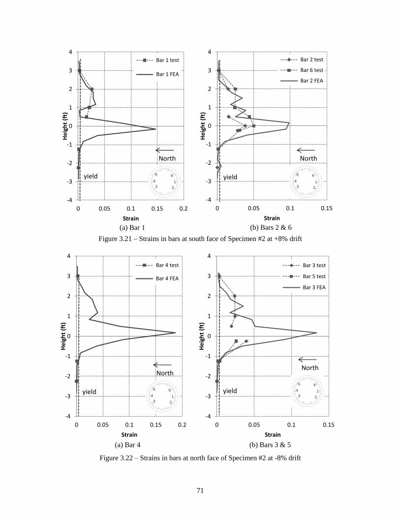
71

Figure 3.21 – Strains in bars at south face of Specimen #2 at +8% drift

Figure 3.22 – Strains in bars at north face of Specimen #2 at -8% drift

-4

-3

-2

-1

0

1

2

3

4

0 0.05 0.1 0.15 0.2

He

igh

t (f

t)

Strain

Bar 1 test

Bar 1 FEA

(a) Bar 1

1

23

4

5 6

North

yield

-4

-3

-2

-1

0

1

2

3

4

0 0.05 0.1 0.15H

eig

ht

(ft)

Strain

Bar 2 test

Bar 6 test

Bar 2 FEA

(b) Bars 2 & 6

1

23

4

5 6

North

yield

-4

-3

-2

-1

0

1

2

3

4

0 0.05 0.1 0.15 0.2

He

igh

t (f

t)

Strain

Bar 4 test

Bar 4 FEA

(a) Bar 4

1

23

4

5 6

North

yield

-4

-3

-2

-1

0

1

2

3

4

0 0.05 0.1 0.15

He

igh

t (f

t)

Strain

Bar 3 test

Bar 5 test

Bar 3 FEA

(b) Bars 3 & 5

1

23

4

5 6

North

yield

72

Figure 3.23 – Axial stress-strain curves from cover concrete and core concrete for Specimen #1

Figure 3.24 –Stress-strain curves for longitudinal bars at the base of the pile of Specimen #1

-9

-8

-7

-6

-5

-4

-3

-2

-1

0

1

-0.1 -0.08 -0.06 -0.04 -0.02 0 0.02 0.04

Axi

al s

tre

ss (

ksi)

Axial strain

cover element

core element

-150

-100

-50

0

50

100

150

-0.1 -0.05 0 0.05 0.1 0.15 0.2 0.25 0.3 0.35 0.4

Axi

al s

tre

ss (

ksi)

Axial strain

bar #1

bar #4

- +

1

23

4

5 6

73

Figure 3.25 – Lateral load-vs.-drift ratio curves for models with D=28 in.

Figure 3.26 – Cycles at which the longitudinal bars fractured for models with D=28 in.

-100

-80

-60

-40

-20

0

20

40

60

80

-15 -10 -5 0 5 10 15

Late

ral l

oad

(ki

ps)

Drift (%)

D28S1 (6 No. 11)

D28S4 (8 No. 10)

D28S2 (10 No. 9)

D28S3 (16 No. 7)

(a) D28S1 (b) D28S4

(c) D28S2 (d) D28S3

1st cycle of -10% 2nd cycle of +10%

2nd cycle of -8% 1st cycle of +10%

1st cycle of -10%

2nd cycle of +10%

2nd cycle of -6%

2nd cycle of +8%

1st cycle of -10%

1st cycle of +8%

1st cycle of -8%

2nd cycle of -8%

1st cycle of +10% 1st cycle of -10%

74

Figure 3.27 – Normal plastic strains in the axial direction at 1% drift for models with D=28 in.

(a) D28S1 (b) D28S4

(c) D28S2 (d) D28S3

12’’

6’’

8’’

6’’

8’’

6’’

8’’

5.6’

8’’

6’’

5’’

10’’

8’’

6’’

6’’

8’’

6’’

6’’

8’’

5’’

8’’

6’’

4’’6’’

6’’

5’’

5’’

7’’

6’’5.9’

8’’

6’’

9’’

5.8’

6.1’

75

Figure 3.28 – Lateral load-vs.-drift ratio curves for models with D=56 in.

Figure 3.29 – Normalized lateral load-vs.-drift ratio curves of pile models with different diameter

-400

-300

-200

-100

0

100

200

300

400

-15 -10 -5 0 5 10 15

Late

ral l

oad

(ki

ps)

Drift (%)

D56S1 (6 No. 14 & 6 No. 18)

D56S2 (10 No. 18)

D56S3 (16 No. 14)

-1.5

-1

-0.5

0

0.5

1

1.5

-0.15 -0.10 -0.05 0.00 0.05 0.10 0.15

F/Fm

ax

Drift (%)

D28S2 (spacing 6.75 in.)D56S2 (spacing 15 in. )

76

Figure 3.30 – Cycles at which the longitudinal bars fractured for models with D=56 in.

(a) D56S1

(b) D56S2 (c) D56S3

2nd cycle of +8% 2nd cycle of +8%

2nd cycle of -8% 1st cycle of +10%

1st cycle of -10%

2nd cycle of +10%

1st cycle of +8%

2nd cycle of +8%

1st cycle of -10%

2nd cycle of -6%

1st cycle of -8%

2nd cycle of -8%

77

Figure 3.31 – Normal plastic strains in the axial direction at 1% drift for models with D=56 in.

20’’

16’’

12’’

10’’

10’’

20’’

8’’

12’’

12.3’

20’’

8’’

12’’8’’

8’’

12’’

8’’8’’

12.7’

12’’

12’’

(a) D56S1

(b) D56S2

12’’

8’’

12’’

8’’12’’8’’

12’’

12’’

12’’

12’’

12.7’

(c) D56S3

78

Figure 3.32 – Normal plastic strains in the axial direction at 1% drift for piles D28S2 and D56S2

Figure 3.33 – Mesh sensitivity study for the normal plastic strains in pile D56S1

20’’

8’’

12’’8’’

8’’

12’’

8’’8’’

12.7’

12’’

12’’

(b) D56S2(c) D28S2

8’’

6’’

6’’

8’’

6’’

6’’

8’’

5’’

5.9’

D = 28 in., H = 10 ft.

Elements height of 2 in.D = 56 in., H = 20 ft.

Elements height of 4 in.

20’’

16’’

12’’

10’’

10’’

20’’

8’’

12’’

(a) 4 in. layer size

22’’

10’’

11’’

12’’

12’’

8’’

12’’

12’’

10’’

(b) 2 in. layer size

79

Figure 3.34 – Lateral load-vs.-drift ratio curves for models with axial load equal to 0.15 c cA f

Figure 3.35 – Lateral load-vs.-drift ratio curves for models with axial load equal to 0.20 c cA f

-80

-60

-40

-20

0

20

40

60

80

-15 -10 -5 0 5 10 15

Late

ral l

oad

(ki

ps)

Drift (%)

D28S1 (6 No. 11)

D28S2 (10 No. 9)

-80

-60

-40

-20

0

20

40

60

80

100

-15 -10 -5 0 5 10 15

Late

ral l

oad

(ki

ps)

Drift (%)

D28S1 (6 No. 11)D28S2 (10 No. 9)

80

Figure 3.36 – FE model of D28S1-B (with PVC inspection tubes)

Figure 3.37 – Lateral load-vs.-top drift curve for Specimen D28S1-B (with voids)

Longitudinal bars

Voids due to placement of

PVC inspection tubes

Loading direction

Axial load

-80

-60

-40

-20

0

20

40

60

80

-15.00 -10.00 -5.00 0.00 5.00 10.00 15.00

Late

ral l

oad

(ki

ps)

Drift (%)

D28S1

D28S1-B (with voids)

81

CHAPTER 4

FINITE ELEMENT ANALYSES WITH MICROPLANE MODEL

FOR CONCRETE

An improved version of the microplane model (M7) for concrete proposed by Caner and Bazant (2013a)

has been implemented in a user-defined subroutine in Abaqus (Simulia 2012). The model can more

accurately simulate the opening and closing of cracks and the confinement effect in concrete than the

damaged-plasticity constitutive model provided by Abaqus (Simulia 2012). The limitations of the

damaged-plasticity model in simulating the aforementioned phenomena were discussed in Section 2.1 of

this report, along with the ad hoc remedies proposed in this study. In this chapter, the key features of the

microplane model implemented in Abaqus and its calibration are described. In this study, the microplane

model has been calibrated and validated with the experimental data of Hurblut (1985) and Mander et al.

(1988). Furthermore, it has been applied to analyze the nonlinear behavior of the RC pile specimens

tested by Papadopoulos and Shing (2014).

4.1 Model formulation

The microplane model is formulated in terms of a constitutive relation between the stress and strain

components defined on a plane, called a microplane, of any orientation in the material (Brocca and Bazant

2000). It is based on the hypothesis that the free energy density of the material is a sum of the free energy

densities associated with microplanes of various orientations. The free energy density for each microplane

is defined as a function of the corresponding strain components, which are derived from the strain tensor

based on a kinematic constraint. The stresses at the micro and macro levels satisfy equilibrium in an

approximate sense by virtue of the principle of virtual work.

82

As shown in Figure 4.1, the direction of a microplane is identified by a unit normal vector n , defined in

the global Cartesian coordinates, 1x , 2x , and 3x . Each microplane has an associated normal strain

component N and two shear strain components, M and L , in directions defined by two orthogonal

unit vectors, m and l , respectively, oriented parallel to the microplane. These strain components are

derived from the strain tensor ε by projections on n , m and l as follows.

, , N ij ij L ij ij M ij ijN L M (4.1)

where

, / 2, / 2ij i j ij i j j i ij i j j iN n n L l n l n M m n m n (4.2)

in which the subscripts , 1,2,3i j , representing the directions along 1x , 2x , and 3x , respectively, ij

denotes the strain tensor, and in , im , and il are projections of unit vectors n ,m , and l on ix . Repeated

indices in the above equations denote summation over , 1,2,3i j , e.g., 1 1 2 2 3 3i ia b a b a b a b .

It is impossible for both the stress and strain components on the microplanes to be projections of the

stress and strain tensors. Therefore, the static equivalence, or equilibrium, between the stress components,

N , L , and M , over all the microplanes and the stress tensor σ are enforced in an approximate

manner using the principle of virtual work (Bazant, 1984) as follows:

2

3ij ij N N L L M M d

(4.3)

in which is the surface of a unit hemisphere centered at the material point, and 2 / 3 is its volume.

The above equation implies that the volume bounded by the microplanes, as shown in Figure 4.1(a), can

be represented by a unit sphere, and that the virtual work of continuum stresses within a unit sphere is

83

equal to the virtual work of the stress components on the surface (microplanes) of the unit sphere. By

substituting N ij ijN ,

L ij ijL , and M ij ijM into the above equation, and noting that the

equation must hold for any virtue strain ij , the following basic equilibrium relation is obtained:

( )

1

36

2

mN

ij ij ijs d w s

(4.4)

where

ij N ij L ij M ijs N L M (4.5)

As shown in Eq. (4.4), the integral is approximated by an optimal Gaussian integration over a spherical

surface (Stroud 1971, Bazant and Oh 1985), which is a weighted sum over mN microplanes of

orientations n , with the weights w

normalized so that 1

1/ 2mN

w

. The implemented microplane

model has 37 microplanes.

The model has four strain-dependent strength (or yield) limits, enforced at the microplane level, called the

stress-strain boundaries. These are the volumetric boundary, b

V , the deviatoric boundary, b

D , the

normal boundary, b

N , and the shear boundary, b

T , which are presented in Figure 4.2. When the stresses

are within the boundaries, the response is elastic. If, during a strain increment, the boundary is exceeded,

the stress is reduced to the boundary keeping the strain constant, as illustrated for the normal stress, N ,

in Figure 4.3.

The volumetric boundary, b

V , is calculated by the following equation:

1/

1 3V k ab

V Ek k e

(4.6)

84

in which E is the elastic modulus of the concrete, and 1k and 3k are parameters that need to be calibrated.

The physical meaning and suggested values of these parameters are presented in Table 4.1. The

volumetric strain, v , for each microplane is calculated from the strain tensor in an incremental manner as

follows:

Δo

V V V (4.7)

where

/ 3 and Δ / 3o o

V kk V kk (4.8)

The superscript o in the above variables denotes the values attained in the previous step. The variable a

in Eq. (4.6) is defined as follows:

20

54

11

co o

I III

e

ka k

k

(4.9)

in which 4k and 5k are parameters whose physical meaning and suggested values are presented in Table

4.1. e is defined as:

0/o

e V NE (4.10)

where max( ,0)x x (the Macauley brackets), o

v is the volumetric stress attained in the previous

step, defined in Eq.(4.23), and 0NE is the undamaged elastic stiffness in the normal direction of the

microplane and is calculated as:

01 2

N

EE

v

(4.11)

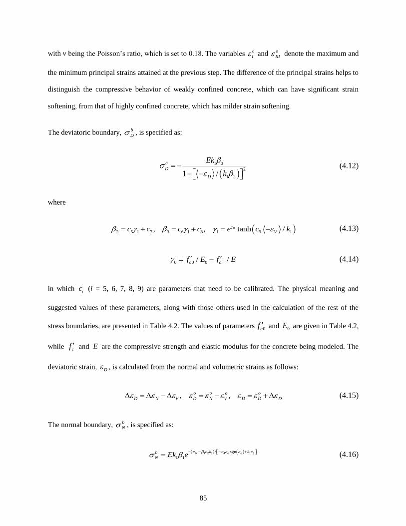
85

with v being the Poisson’s ratio, which is set to 0.18. The variables o

I and o

III denote the maximum and

the minimum principal strains attained at the previous step. The difference of the principal strains helps to

distinguish the compressive behavior of weakly confined concrete, which can have significant strain

softening, from that of highly confined concrete, which has milder strain softening.

The deviatoric boundary, b

D , is specified as:

1 3

2

1 21 /

b

D

D

Ek

k

(4.12)

where

0

2 5 1 7 3 6 1 8 1 9 1, , tanh /Vc c c c e c k (4.13)

0 0 0/ /c cf E f E (4.14)

in which ic (i = 5, 6, 7, 8, 9) are parameters that need to be calibrated. The physical meaning and

suggested values of these parameters, along with those others used in the calculation of the rest of the

stress boundaries, are presented in Table 4.2. The values of parameters 0cf and 0E are given in Table 4.2,

while cf and E are the compressive strength and elastic modulus for the concrete being modeled. The

deviatoric strain, D , is calculated from the normal and volumetric strains as follows:

, , o o o o

D N V D N V D D D (4.15)

The normal boundary, b

N , is specified as:

1 2 1 4 1 3/ sgn

1 1

N e ec k c k cb

N Ek e

(4.16)

86

in which

19 18

1 1 17ec c

c c e

(4.17)

The elastic normal microplane stress (trial elastic stress) is calculated as:

e o

N N N NE (4.18)

in which NE is the damaged value of the normal microplane elastic stiffness:

0

13

0 ( ) for 0Nc o

N N NE E e f

(4.19)

but

0 0 if and 0o o

N N N N N N NE E E (4.20)

014 15/ 1

0 16 for 0N ec c o

N N e NE E e c

(4.21)

in which 0

N and 0

N are the maximum and minimum normal strains reached so far. In Eq. (4.19),

1

2( ) 1f a

, with vd and 0.1a , which has been specified to avoid negative

dissipation during load cycles. Accurate simulation of the closing of opened cracks during tensile

unloading is attained with the stiffness degradation calculated with Eq. (4.19). Parameter 13c controls the

unloading slope from tension, with a suggested value of 4,500 (see Table 4.2). Only those microplanes

whose normals form a sufficiently small angle with the maximum principal strain direction can reach the

post-peak regime. Other microplanes will remain elastic.

87

Having calculated the elastic normal stress and the volumetric, deviatoric and normal stress boundaries,

the vertical drop of stress at constant strain to the stress-strain boundary for the normal stress, as shown in

Figure 4.3, is enforced:

max min , ,e b b b

N N N V D

(4.22)

The volumetric stress is calculated as the average value of the normal stress at every microplane:

1

1

2

mN

V Nw

(4.23)

The shear boundary, b

T , is calculated as:

1

1 1

10 1 2ˆ for 0b o

T N N T Nc E k k

(4.24)

1

1 1

10 1 2ˆ for 0b o

T N T Nc E k k

(4.25)

in which

0

1 4

1T N

vE E

v

(4.26)

1 11 12

ˆ o

N T VE k c c (4.27)

The elastic shear microplane stress (trial stress) is:

2 2

e o o

T L T L M T ME E (4.28)

88

in which o

L and o

M are the shear stresses in the L and M directions of the microplane in the previous

step, and L , M the equivalent strain increments.

The shear stress return to the boundary is calculated by the following equations:

min ,b e

T T T (4.29)

/o e

L L T L T TE (4.30)

/o e

M M T M T TE (4.31)

Having calculated the normal stress , N , and the shear-stress components, L and M , at every

microplane, the stress tensor, ij , at every integration point is obtained through Eq. (4.4) and (4.5).

The fact that the stress-strain boundaries are reached at different microplanes at different moments of

loading is what causes both the pre-peak and post-peak macro-level stress-strain curves to vary their slope

gradually. Similarly during macroscopic unloading, different microplanes have the stresses returning into

the elastic domain at different moments, which again causes the unloading curves to change the unloading

slope gradually.

The calibration of the microplane model involves the determination of the parameters E , ik and jc ,

which govern the stress-strain boundaries at every microplane. The values shown in Table 4.1 and Table

4.2 are suggested by Caner and Bazant (2013b), and will result in a uniaxial compressive strength of 46.7

MPa and the compressive strain at the peak stress equal to 0.0033, which can be confirmed numerically.

To have a different concrete strength, strain at the peak stress, and post-peak behavior under uniaxial

compression, the values of E and ik have to be changed, while those of jc can remain the same.

89

In fact, with the set of parameters that determine the reference concrete properties, the desired uniaxial

compressive strength, cf , and compressive strain at the peak stress, p , can be obtained solely with the

values of 1k and E calculated with the following equations:

1 1 and p pc

p pc

fk k E E

f

(4.32)

in which 1k and E are the values of the parameters that result in the reference properties cf , and p .

For the parameters shown in Table 4.1 and Table 4.2, we have 4

1 1.1 10k , 25,000 MPaE ,

46.7 MPacf , and = 0.0033p . Changing the value of E results in a vertical scaling transformation

of the stress-strain curve, such that all the stresses are scaled by the ratio /E E with no change of strains.

Changing the value of 1k results in a radial scaling of the stress-strain curve, in which all the distances

from the origin are scaled by the ratio 1 1/k k .

4.2 Validation and Calibration of the Microplane model

The microplane model has been calibrated and verified by Caner and Bazant (2013b) for a range of strain

histories. In this study, the performance of the model in capturing the compressive behavior of confined

concrete has been further examined. For this purpose, the tests of Hurblut (1985) on the compressive

behavior of concrete under different lateral confining stresses, the test by van Mier (1986) on the uniaxial

compressive behavior of unconfined concrete, and the tests of Mander et al. (1988b) on the compressive

behavior of circular columns with different amounts of lateral steel confinement are considered. For these

analyses, the default values of some of the modeling parameters have been changed as shown in Table

4.3.

90

The finite element (FE) model used to simulate the tests of Hurblut (1985) is presented in Figure 2.8. The

default values of ik for 2,...,5i and jc for 1,...,20j , which are presented in Table 4.1 and

Table 4.2, are first used, while 26,030 MPaE and 4

1 0.5 10k (see Table 4.3), which have been

selected to capture the compressive behavior of the concrete. As shown in Figure 4.4, the microplane

model is capable of reproducing the effect of the lateral confining stress on the compressive strength and

the post-peak slope of the stress-strain curve. However, for the case of uniaxial compression with no

confining stress, the microplane model shows a relatively ductile behavior, with the stress-strain curve

similar to that for the 100-psi confining stress. To examine this further, the uniaxial compression test of

van Mier (1986) is considered. As shown in Figure 4.5, the microplane model demonstrates a more

ductile post-peak behavior than the test. To have a more brittle behavior under uniaxial compression, the

model has been re-calibrated with the values of 2k and 3k changed to one. With 2 3 1k k ,

27,865 MPaE , and 4

1 1.65 10k , the model gives 21.4 MPacf and = 0.0015p . As shown

in Figure 4.5, this results in a much better match of the test data. This value of 2k and 3k is used for

unconfined concrete in all subsequent analyses, as shown in Table 4.3.

With the aforementioned recalibration, the microplane model was further evaluated with the experimental

results of Mander et al. (1988b) on the compressive behavior of circular-sectioned RC columns with

different amounts of lateral confining steel. The calibration of the model to yield the concrete properties

of the tests is summarized in Table 4.3. The same FE model as that presented in Figure 2.12 is used.

However, in contrast to the damaged-plasticity model, which requires different input uniaxial

compressive stress-strain relations for different amounts of confining steel, as discussed in Chapter 2, the

microplane model uses the same calibration for different confinement levels. As shown in Figure

4.6Figure 4.6, the FE model satisfactorily captures the effect of the lateral confining steel on the

compressive strength and the ductility of the RC columns.

91

Unlike the damaged-plasticity model provided in Abaqus (Simulia, 2012), the microplane model is able

to simulate the tensile unloading and reloading behavior of concrete in an accurate manner. To

demonstrate this, a single solid element, as shown in Figure 4.7, is subjected to uniaxial cyclic tension and

compression. Both the damaged-plasticity model and the microplane model are considered. Figure 4.8

shows the stress-strain curves obtained with the two different constitutive models. It can be seen that the

damaged-plasticity model shows early crack closing with an unrealistically large residual tensile strain

due to its inability to represent severe degradation of the tensile stiffness during unloading, as pointed out

in Chapter 2, while the microplane model shows a satisfactory performance.

4.3 Finite Element Analysis of pile specimens with the microplane model

The microplane model is used in the finite element analysis of the pile specimens tested by Papadopoulos

and Shing (2014). As shown in Figure 4.9, the FE model for the pile specimens is similar to the one

presented in Section 3.1, except that the contact conditions at the pile-footing interface have been

eliminated. This is because the microplane model can adequately simulate the opening and closing of

flexural cracks. Table 4.3 summarizes the values of E and 1k selected to match the properties of the

concrete in the piles. The longitudinal bars and the confining hoops are modeled in the same way as that

presented in Section 3.1. Bond-slip between the concrete and the longitudinal bars is also modeled in the

same manner.

4.3.1 Specimen #1

Figure 4.10 shows the lateral load-vs.-top drift curves obtained for Specimen #1 by the test and the FE

model. The curve form the FEA matches the test result well in terms of the lateral-load capacity, the post-

peak behavior, and the pinching due to the opening and closing of flexural cracks. The drop of the lateral-

load resistance at the 2nd

cycle of 10% drift, due to the fracture of the longitudinal bars, is also reproduced

by the FEA with the use of the phenomenological LCF law for steel presented in Section 2.2.2. Figure

92

4.11 shows the deformed shape of Specimen #1 at the end of the 2nd

cycle of 10% drift. With the

elimination of the contact conditions at the pile-footing interface, flexural cracking tends to largely

concentrate in the first layer of the concrete elements at the base of the pile. The opening and closing of

flexural cracks is accurately simulated. Figure 4.12 and Figure 4.13 show the axial stress-strain responses

of concrete cover and core elements at the toe of the pile in Specimen #1. The microplane model is

capable of accurately simulating the opening and closing of flexural cracks.

As shown in Figure 4.12, an element in the concrete cover experiences large tensile strains, which goes

back to almost zero before developing a maximum compressive stress of 6 ksi, which is slightly larger

than the prescribed unconfined compressive strength of 5 ksi. This slight increase in strength can be

attributed to the confinement effect provided by the footing. Similar observations can be made for an

element in the concrete core, which develops a high compressive stress of 9 ksi due to the confinement

provided by the transverse reinforcement.

Table 4.4 summarizes the cycles in which the longitudinal bars of Specimen #1 fractured in the test and in

the FEA, showing a close correlation of the experimental and numerical results. The positions of Bars 1

and 4, along with the cycles in which they fracture in the FEA, are shown in Figure 4.14.

The strains in the longitudinal bars on the south side of the pile at different drift levels are plotted in

Figure 4.17 through Figure 4.19. The strains predicted in the FEA are compared to the test results in these

plots. In general, the numerical results match the test data well. However, at locations close to the pile-

footing interface, the tensile strain in Bar 1, which is at the extreme position on the south side, at pile drift

ratios of 1% and 4% is significantly over-estimated in the FEA. As discussed in Sec. 3.2.3, one possible

explanation is that the damage of the concrete and the bond at the base of the pile at these drift levels can

be slightly under-estimated by the FE model and the tensile strain in a bar is highly sensitive to the

damage. It is interesting to note that the FEA accurately captures the strains in the longitudinal bars

embedded inside the footing.

93

4.3.2 Specimen #2

Specimen #2, which consisted of 10 No. 9 longitudinal bars, is also modeled with the microplane model.

Figure 4.15 shows the good match of the lateral load-vs.-top drift curves obtained from the test and the

FEA. The numerical results for Specimen #2 are similar to those for Specimen #1. Table 4.5 summarizes

the cycles in which the bars fractured in the test and in the FEA. The FE model is able to accurately

predict the LCF of the longitudinal bars. Figure 4.16 shows the positions of the longitudinal bars, along

with the cycles in which the bars fractured.

Similar to the analyses presented in Chapter 3, the results here show that the difference in the lineal

spacing of longitudinal bars for the two specimens does not have any effect on the ductility of the lateral

load-vs.-drift ratio response. The size of the longitudinal bars, however, can have an effect to the ductility

of the pile. The No. 9 longitudinal bars of Specimen #2, fractured earlier than the No. 11 longitudinal bars

of Specimen #1. Smaller-diameter bars are less resistant to buckling for the same spacing of the

transverse reinforcement, and can therefore lead to a less ductile behavior of a laterally loaded RC

member.

The strains in the longitudinal bars placed on the south side of the pile at different drift levels are shown

in Figure 4.20 through Figure 4.22. Expect for some discrepancies observed at the pile-footing interface,

like those observed for Specimen 1, the strains in the longitudinal bars obtained from the FE model

satisfactorily match the experimental data.

4.3.3 Flexural Crack Pattern

Figure 4.23 shows the normal strains developed in concrete, in the axial direction of the pile, at a drift

ratio of 1% in the FEA of the two pile specimens. In this figure, flexural cracks can be identified as

localized tensile strains. The maximum tensile strains developed in Specimen #1 are larger than those in

Specimen #2, consistent with the experimental observations. Moreover, the flexural cracks in Specimen

94

#2 spread over a larger distance than those in Specimen #1. However, the spacings of the flexural cracks

are more or less the same for the two cases, with Specimen #2 showing a slightly smaller spacing between

the first two cracks near the base.

4.4 Summary and Conclusions

The new microplane model developed by Caner and Bazant (2013a) has been implemented in a user-

defined subroutine in Abaqus (Simulia 2012) and has been calibrated and verified with the tests of

Hurblut (1985), van Mier (1986) and Mander et al. (1988b). It has been employed to analyze the

nonlinear behavior of the RC pile specimens tested by Papadopoulos and Shing (2014). The microplane

model can simulate the nonlinear behavior of concrete more accurately than the damaged-plasticity

model. More specifically, it can adequately represent large stiffness degradation during unloading and

reloading in tension. Thus, the finite element models can accurately capture the pinching effect in the

load-displacement curve for a pile. Furthermore, the microplane model can accurately reproduce both the

enhanced compressive strength and the more ductile post-peak behavior of confined concrete. The

damaged-plasticity model can only reproduce the enhanced compressive strength but not the enhanced

ductility of confined concrete. Even though this limitation of the damaged-plasticity model can be

artificially circumvented by modifying the input uniaxial compressive behavior of concrete, the remedy is

far from exact. It cannot represent the variation of confinement pressure across a member section. While

this may not be an important issue for tension-controlled flexural members, it can lead to inaccurate

results for compression-controlled members, such as members subjected to high axial loads.

95

Table 4.1 – Free parameters of microplane model by Caner and Bazant (2013b)

Parameter Value Description

v 0.18 Poisson’s ratio

E 25,000 MPa Elastic modulus

1k 41.1 10 Radial scaling parameter

2k 110 Controls the horizontal asymptote value in the shear boundary

3k 30 Controls the shape of the volumetric boundary

4k 100 Controls the shape of the volumetric boundary

5k 0.0001 Controls the volumetric-deviatoric coupling at low pressures

Table 4.2 – Fixed parameters of microplane model by Caner and Bazant (2013b)

Parameter value meaning

0cf 15.1 MPa Reference compressive strength for low-strength concrete

0E 20,000 MPa Reference elastic modulus for low-strength concrete

c1 0.089 Controls the uniaxial tensile strength

c2 0.176 Controls the roundness of the peak in uniaxial tension

c3 4 Controls the slope of the post-peak tail in uniaxial tension

c4 50 Controls the slope of the post-peak tail in uniaxial compression

c5 3,500 Controls the volumetric expansion under compression

c6 20 Controls the roundness of the peak in volumetric expansion under

compression

c7 1 Controls the slope of the initial post-peak curve in uniaxial

compression

c8 8 Controls the peak strength in uniaxial compression

c9 0.012 Controls the peak roundness in uniaxial compression

c10 0.33 Controls the effective friction coefficient

c11 0.5 Initial cohesion in frictional response

c12 2.36 Controls the change of cohesion with tensile volumetric strains

c13 4,500 Controls the unloading slope in tension

c14 300 Controls the unloading slope at low hydrostatic compression

c15 4,000 Controls the transition from unloading slope at high confinement to

that at low confinement

96

c16 60 Controls the unloading slope at high hydrostatic compression

c17 1.4 Controls the tensile strength

c18 0.0016 Controls the tensile cracking under compression

c19 1,000 Controls the tensile softening rate under compression

c20 1.8 Controls the volumetric-deviatoric coupling at high pressures

Table 4.3 – Calibration of microplane model

Test Concrete 2 3,k k E (MPa) 1k (x10-4

) cf (MPa),

p

Hurblut (1985) Confined default 26,030 0.5 22.1, 0.0015

van Mier (1986) Unconfined default 25,200 0.5 21.4, 0.0015

Unconfined 1, 1 27,865 1.65 21.4, 0.0015

Mander et al.

(1988b)

Confined default 34,035 0.5 28.9, 0.0015

Unconfined 1, 1 37,630 1.65 28.9, 0.0015

Papadopoulos

and Shing (2014)

Confined default 40,630 0.5 34.5, 0.0015

Unconfined 1, 1 44,920 1.65 34.5, 0.0015

Table 4.4 – Cycles at which bars fractured in Specimen #1

Bar no. Bar fracture in test Bar fracture in FEA

1 2nd

cycle at +10% 1st cycle at -10%

4 2nd

cycle at -10% 2nd

cycle at +10%

Table 4.5 – Cycles at which bars fractured in Specimen #2

Bar no. Bar fracture in test Bar fracture in FEA

1 1st cycle at +10% 2

nd cycle at +8%

4 1st cycle at -10% 2nd cycle at -8%

3, 5 1st cycle at -10% 1

st cycle at -10%

2, 6 no fracture 2nd

cycle at +10%

97

Figure 4.1 – (a) System of discrete microplanes, (b) Microplane strain vector and its components (Caner

and Bazant, 2013a)

Figure 4.2 – Stress-strain boundaries of the microplane model (Caner and Bazant, 2013a)

(a) Normal boundary (c) Deviatoric boundary

(b) Volumetric boundary (d) Shear boundary

(a) (b)

M

98

Figure 4.3 – Vertical return to normal boundary when the boundary is exceeded by an elastic trial stress in

a finite load step (Caner and Bazant, 2013a)

Figure 4.4 – Comparison of microplane model with default parameters to experimental results by Hurblut

(1985)

No

N N o

N

N

el

N

o

N

N

N

-6

-5

-4

-3

-2

-1

0

-0.020 -0.015 -0.010 -0.005 0.000 0.005 0.010 0.015 0.020

Stre

ss (

ksi)

100 psi (test)

500 psi (test)

unconfined concrete (FEA)

100 psi (FEA)

500 psi (FEA)

axial strain lateral strain

99

Figure 4.5 – Comparison of microplane model to uniaxial compression test by van Mier (1986)

-3.5

-3

-2.5

-2

-1.5

-1

-0.5

0

-0.020 -0.015 -0.010 -0.005 0.000

Stre

ss (

ksi)

Strain

Test with uniaxial compression (van Mier, 1986)

Model with modified parameters

Model with default parameters

k2=1, k3=1

100

Figure 4.6 – Comparison of microplane model to experimental results by Mander et al. (1988b)

0

5

10

15

20

25

30

35

40

45

0.000 0.005 0.010 0.015 0.020

Stre

ss (

MP

a)

Strain

ρv=0.6% test (Mander et al. 1988b) ρv=0.6% (microplane model) ρv=0 test

ρs=0 microplane

(a) ρs=0.6%

ρs = 0.6% Test

ρs = 0.6% FEA (microplane model)

ρs = 0 Test

ρs = 0 FEA (microplane model)

0

10

20

30

40

50

60

0.000 0.005 0.010 0.015 0.020

Stre

ss (

MP

a)

Strain

ρv=2.5% test (Mander et al., 1988b) ρv=2.5% (microplane model) ρv=0 test

ρv=0 microplane

(b) ρs=2.5%

ρs = 2.5% Test

ρs = 2.5% FEA (microplane model)

ρs = 0 Test

ρs = 0 FEA (microplane model)

101

Figure 4.7 – Model for cyclic loading in tension

Figure 4.8 – Comparison of microplane model and D-P model under cyclic loading in tension

-6

-5

-4

-3

-2

-1

0

1

0 0.001 0.002 0.003 0.004 0.005 0.006

Stre

ss (

ksi)

Strain

Microplane model

D-P model

102

Figure 4.9 – FE model of Specimen #1 assembly with microplane model for concrete

Longitudinal bar

Bond-slip interface

element

Concrete

Microplane model for

unconfined concrete

Microplane model for

confined concrete

Reinforcement cage

Elastic concrete for footing

Axial load and lateral

displacement applied at

the top of the cap, which

is modeled with elastic

concrete elements

Long. bars modeled

with beam elements

Hoops modeled

with truss elements

103

Figure 4.10 – Lateral load-vs.-top drift ratio curves for Specimen #1

Figure 4.11 – Deformed shape of FE model of Specimen #1 at 10% drift

-80

-60

-40

-20

0

20

40

60

80

-15 -10 -5 0 5 10 15

Forc

e (k

ips)

Drift (%)

TestFEA (microplane…

104

Figure 4.12 – Axial stress-strain curve for cover concrete at the base of Specimen #1

Figure 4.13 – Axial stress-strain curve for core concrete at the base of Specimen #1

-7

-6

-5

-4

-3

-2

-1

0

1

2

-0.1 0.0 0.1 0.2 0.3 0.4 0.5 0.6 0.7 0.8

Str

ess

(ksi

)

Strain

-10

-8

-6

-4

-2

0

2

-0.04 -0.02 0.00 0.02 0.04 0.06 0.08 0.10 0.12 0.14 0.16

Str

ess

(ksi

)

Strain

105

Figure 4.14 – Cycles at which bars fracture in the FEA of Specimen #1

Figure 4.15 – Lateral load-vs.-top drift ratio curves for Specimen #2

Figure 4.16 – Cycles at which bars fracture in the FEA of Specimen #2

2nd cycle of +10% 1st cycle of -10%

-100

-80

-60

-40

-20

0

20

40

60

80

100

-15 -10 -5 0 5 10 15

Forc

e (

kip

s)

Drift (in.)

Test

1st cycle of -10%

2nd cycle of -8%

1st cycle of +10%

2nd cycle of +8%

106

Figure 4.17 – Strains in bars at south face of Specimen #1 at +1% drift

Figure 4.18 – Strains in bars at south face of Specimen #1 at +4% drift

-4

-3

-2

-1

0

1

2

3

4

0 0.005 0.01

He

igh

t (f

t)

Strain

bar 1 test

bar 1 FEA(microplane)

(b) Bar 1

yield 1

23

4

5 6

+

-4

-3

-2

-1

0

1

2

3

4

0 0.001 0.002 0.003 0.004

He

igh

t (f

t)

Strain

bar 2 test

bar 6 test

bar 2 FEA(microplane)

(a) Bar 2 & 6

yield

1

23

4

5 6

+

-4

-3

-2

-1

0

1

2

3

4

0 0.02 0.04 0.06

He

igh

t (f

t)

Strain

bar 1 test

bar 1 FEA(microplane)

(a) Bar 1

yield

1

23

4

5 6

+

-4

-3

-2

-1

0

1

2

3

4

-0.01 0.01 0.03 0.05

He

igh

t (f

t)

Strain

bar 2 test

bar 6 test

bar 2 FEA(microplane)

(b) Bars 2 & 6

+

yield 1

23

4

5 6

107

Figure 4.19 – Strains in bars at the south face of Specimen #1 at +8% drift

Figure 4.20 – Strains in bars at south face of Specimen #2 at +1% drift

-4

-3

-2

-1

0

1

2

3

4

0 0.02 0.04 0.06 0.08 0.1

He

igh

t (f

t)

Strain

bar 1 test

bar 1 FEA(microplane)

(a) Bar 1

yield

1

23

4

5 6

+

-4

-3

-2

-1

0

1

2

3

4

0 0.02 0.04 0.06 0.08H

eig

ht

(ft)

Strain

bar 2 test

bar 6 test

bar 2 FEA(microplane)

(b) Bars 2 & 6

yield

1

23

4

5 6

+

-4

-3

-2

-1

0

1

2

3

4

0 0.005 0.01 0.015

He

igh

t (f

t)

Strain

bar 1 test

bar 1 FEA(microplane)

(a) Bar 1

yield 1

23

4

5 6

+

-4

-3

-2

-1

0

1

2

3

4

0 0.005 0.01 0.015

He

igh

t (f

t)

Strain

bar 2 test

bar 6 test

bar 2 FEA(microplane)

(b) Bars 2 & 6

1

23

4

5 6

yield

+

108

Figure 4.21 – Strains in bars at south face of Specimen #2 at +4% drift

Figure 4.22 – Strains in bars at south face of Specimen #2 at +8% drift

-4

-3

-2

-1

0

1

2

3

4

0 0.02 0.04 0.06

He

igh

t (f

t)

Strain

bar 1 test

bar 1 FEA(microplane)

(a) Bar 1

yield 1

23

4

5 6

+

-4

-3

-2

-1

0

1

2

3

4

0 0.01 0.02 0.03 0.04H

eig

ht

(ft)

Strain

bar 2 test

bar 6 test

bar 2 FEA(microplane)

(b) Bars 2 & 6

yield 1

23

4

5 6

+

-4

-3

-2

-1

0

1

2

3

4

0 0.02 0.04 0.06 0.08

He

igh

t (f

t)

Strain

bar 1 test

bar 1 FEA(microplane)

(a) Bar 1

yield 1

23

4

5 6

+

-4

-3

-2

-1

0

1

2

3

4

0 0.02 0.04 0.06 0.08

He

igh

t (f

t)

Strain

bar 2 test

bar 6 test

bar 2 FEA(microplane)

(b) Bars 2 & 6

yield 1

23

4

5 6

+

109

Figure 4.23 – Normal strains in concrete at 1% drift

(a) Specimen #1 (b) Specimen #2

110

CHAPTER 5

SUMMARY AND CONCLUSIONS

5.1 Summary

This report presents a numerical investigation of the influence of the spacing of longitudinal bars on the

structural performance of circular RC pile shafts. Three-dimensional nonlinear finite element (FE) models

have been developed for RC pile shafts, and used for a numerical parametric study to confirm and

generalize the experimental observations from the two pile specimens tested by Papadopoulos and Shing

(2014). The modeling method has been validated by the experimental data. For the finite element

analysis, a phenomenological stress-strain law for steel has been developed, accounting for the low-cycle

fatigue of bars under large-amplitude cyclic strain reversals.

The damaged-plasticity model provided in Abaqus has been used to model the behavior of concrete. It is

based on the model proposed by Lubliner et al. (1989) and modified by Lee and Fenves (1998). Two

limitations of the model have been identified and remedies have been developed to partially circumvent

them. The first limitation is that the model cannot capture the increase in the ductility of concrete in

compression as the confinement pressure increases. To circumvent this limitation, the slope of the

decaying branch of the input uniaxial compressive stress-strain curve has to be modified a priori based on

the level of the confinement pressure or the amount of the confinement steel. The second limitation is that

the model is not able to represent large stiffness degradation during unloading and reloading in tension,

resulting in a large residual tensile strain upon unloading when large crack opening has occurred. This

prevents the finite element models from accurately capturing the pinching effect in the load-displacement

curve for a pile. To overcome this problem, contact conditions have to be introduced to represent major

flexural cracks in a discrete manner.

111

In view of the aforementioned problems of the damaged-plasticity model, a new microplane model for

concrete developed by Caner and Bazant (2013a) has been implemented in Abaqus. It does not have the

deficiencies identified with the damaged-plasticity model. The calibration of the microplane model has

been improved to simulate the compressive behavior of unconfined concrete more accurately, and the

model has been successfully used to capture the behavior of the two pile specimens.

A phenomenological bond-slip law, developed by Murcia-Delso and Shing (2013), has been used to

model the bond-slip behavior between the longitudinal bars and the surrounding concrete. The parametric

study considers piles of different diameters, with different lineal and angular spacings of the longitudinal

bars, and with different levels of the axial load.

5.2 Conclusions

The finite element models developed here can adequately reproduce the behavior of two circular RC pile

shafts tested in the laboratory. A numerical parametric study has been conducted with finite element

models. The study has confirmed the experimental findings that the lineal spacing of the longitudinal bars

does not have any impact on the ductility of an RC circular pile. The spacing can be larger than the 8-in.

maximum permitted by the Caltrans and AASHTO specifications without compromising the structural

performance of the circular RC member. However, from the standpoint of construction convenience and

assuring consistent behavior under lateral loading in any direction, the specification in Section 8.18.1.2 of

Caltrans Bridge Design Specifications (2004) that the number of longitudinal bars shall not be less than

six (6) is reasonable. This implies that the angular spacing for longitudinal bars should be no greater than

60o, which is also the largest considered in this study.

The size of the longitudinal bars can affect the ductility of a pile, for the same spacing of the lateral

reinforcement. The load degradation in a pile is often associated with the spalling of the cover concrete,

and the buckling and the fracture of the longitude bars in the plastic-hinge region of the pile. Larger-

112

diameter bars are more resistant to buckling for the same spacing of the lateral reinforcement and

therefore result in a more ductile behavior. The parametric study has also confirmed that a smaller lineal

spacing with smaller-size longitudinal bars can lead to more closely spaced flexural cracks with smaller

widths. Furthermore, the voids introduced at the locations of the PVC inspection tubes do not have

significant impact on the nonlinear behavior of the piles. These observations are true for piles of different

diameters and subjected to different levels of axial loads.

113

REFERENCES

Aktan, A. E., Karlsson, B. I., Sozen, M. A. (1973), “ Stress-Strain Relationships of Reinforcing Bars

Subjected to Large Strain Reversals”, Report UILU-ENG-73-2014, University of Illinois at Urbana-

Champaign.

AASHTO (2014), AASHTO LRFD Bridge Design Specifications, 5th Edition, American Association of

State Highway and Transportation Officials, Washington, DC.

Bazant, Z. P. (1984), “Microplane model for strain-controlled inelastic behavior”, J. Wiley, London,

Chapter 3, pp. 45-59, edited by C.S. Desai and R. H. Gallagher.

Bazant, Z. P. and Oh, B. H. (1985), “Microplane model for progressive fracture of concrete and rock”,

Journal of Engineering Mechanics, ASCE, 111, 559-582

Brocca, F. C. and Bazant, Z. P. (2000), “Microplane constitutive model and metal plasticity”, ASME

Applied Mechanics Reviews, 53(10), pp. 265-281.

Brown, J. and Kunnath, S. K. (2004), “Low-cycle Fatigue Behavior of Reinforcing Bars”, ACI Materials

Journal, Vol. 101, No. 6, pp. 457-466.

Caner, F. C. and Bazant, Z. P. (2013a), “Microplane Model M7 for Plain Concrete. I: Formulation”, J.

Eng. Mech., 139(12), pp. 1714-1723.

Caner, F. C. and Bazant, Z. P. (2013b), “Microplane Model M7 for Plain Concrete. II: Calibration and

Verification”, J. Eng. Mech., 139(12), pp. 1724-1735.

Caltrans (2004), Bridge Design Specifications, California Department of Transportation, Sacramento, CA.

Coffin, L. F., Jr., (1954), “A Study of the Effects of Cyclic Thermal Stresses in a Ductile Metal”, ASME

Transactions, Vol. 16, pp. 931-950.

Dhakal, R., and Maekawa, K. (2002), “Modeling for Postyield Buckling of Reinforcement”, J. Struct.

Eng., 18, pp. 1139-1147.

Dodd, L. L., Restrepo-Posada, J. I. (1995), “Model for Predicting Cyclic Behavior of Reinforcing Steel”,

Journal of Structural Engineering, Vol. 121, No. 3, pp. 433-445.

Drucker, D. C., Prager, W. (1952), “Soil Mechanics and Plastic Analysis or Limit Design”, Quarterly of

Applied Mathematics, Vol. X, No. 2, pp. 157-165.

Eligehausen, R., Popov, E. P., Bertero, V. V. (1983), “Local Bond Stress-Slip Relationships of Deformed

Bars under Generalized Excitations”, Report No. UCB/EERC-83/23, Earthquake Engineering Research

Center, University of California, Berkeley.

114

Filippou, F. C., Bertero, V. V., Popov, E. P. (1983), “Effects of Bond Deterioration on Hysteretic

Behavior of Reinforced Concrete Joints”, Report No. UCB/EERC-83/19, University of California,

Berkeley.

Hurblut, B. J. (1985), “Experimental and computational investigation of strain-softening in concrete”, MS

Thesis, University of Colorado, Boulder, CO.

Karthik, M. M., Mander, J. B. (2011), “Stress-Block Parameters for Unconfined and Confined Concrete

Based on a Unified Stress-Strain Model”, Journal of Structural Engineering, pp. 270-273.

Kent, D. C., Park, R. (1973), “Cyclic Load Behavior of Reinforcing Steel” Strain, Vol. 9, No. 3, pp. 98-

103.

Koh, S. K. and Stephens, R. I. (1991), “Mean Stress Effects on Low-cycle Fatigue for a High Strength

Steel”, Journal of Fatigue Fracture of Engineering Materials, Vol. 14, No. 4, pp.413-428.

Kunnath, S., Heo, Y., and Mohle, J. (2009a), “Nonlinear Uniaxial Material Model for Reinforcing Steel

Bars”, J. Struct. Eng., 135(4), pp. 335-343.

Kunnath. S. K., Kanvinde, A., Xiao, Y., Zhang, G. ( 2009b), “Effects of Buckling and Low-cycle Fatigue

on Seismic Performance of Reinforcing Bars and Mechanical Couples for Critical Structural Members”,

Report No. UCD-SESM-08-01, University of California at Davis.

Lee, J., Fenves, G. L. (1998), “Plastic-Damage Model for Cyclic Loading of Concrete Structures”,

Journal of Engineering Mechanics, pp. 892-900.

Lowes, L.N., Moehle, J.P., Govindjee, S. (2004), “Concrete-Steel Bond Model for Use in Finite Element

Modeling of Reinforced Concrete Structures,” ACI Structural Journal, Vol. 101, No. 4, pp. 501-511.

Lubliner, J., Oliver, J., Oller, S., Onate, E. (1989), “A Plastic-Damage Model for Concrete”, International

Journal of Solids and Structures, Vol. 25, No. 3, pp. 299-326.

Mander, J. B., Priestley, M. J. N., Park, R. (1988a), “Theoretical Stress-Strain Model for Confined

Concrete” Journal of Structural Engineering, Vol. 114, No. 8, pp. 1804-1826.

Mander, J. B., Priestley, M. J. N., Park, R. (1988b), “Observed Stress-Strain Behavior pf Confined

Concrete” Journal of Structural Engineering, Vol. 114, No. 8, pp. 1827-1849.

Manson, S. S. (1953), “Behavior of Materials under Conditions of Thermal Stresses”, Heat Transfer

Symposium, University of Michigan Engineering Research Institute, Ann Arbor, Michigan

Menegotto, M., Pinto, P. E. (1973), “Method of Analysis for Cyclically Loaded Reinforced Concrete

Plane Frames Including Changes in Geometry and Non-Elastic Behavior of Elements under Combined

Normal Force and Bending”, IABSE Symposium on Resistance and Ultimate Deformability of Structures

Acted on by Well-Defined Repeated Loads, Final Report, Lisbon.

115

Miner, M. A. (1945), “Cumulative Damage in Fatigue”, Journal of Applied Mechanics, Vol. 12, No. 3,

pp.159-164.

Monti, G., Nuti, C. (1992), “Nonlinear Cyclic Behavior of Reinforcing Bars Including Buckling”, Journal

of Structural Engineering, Vol.118, No. 12, pp. 3268-3284.

Murcia-Delso, J., and Shing, P. B. (2015), “Bond-Slip Model for Detailed Finite-Element Analysis of

Reinforced Concrete Structures”, J. Struct. Eng., 141(4), 04014125.

Ottosen, N. S. (1977), “A Failure Criterion for Concrete”, Journal of the Engineering Mechanics

Division, Vol. 103, No. 4, pp 527-535.

Papadopoulos, V., Shing, P. B. (2014), “Influence of the Spacing of Longitudinal Reinforcement on the

Performance of Laterally Loaded CIDH Piles – Experimental Investigation”, Report No. SSRP-14/08,

University of California, San Diego.

Paulay, T., Priestley, M. J. N. (1992), Seismic Design of Reinforced Concrete and Masonry Buildings,

John Wiley & Sons, Inc.

Pochanart, S., Harmon, P. (1989), “Bond-Slip Model for Generalized Excitations Including Fatigue”, ACI

Materials Journal, Vol. 86, No. 5, pp. 465-474.

Simulia (2012), Abaqus V. 6.10, Dassault Systems Simulia Corp., Providence, RI.

Stroud, A. H. (1971), “Approximate Calculation of Multiple Integrals”, Prentice-Hall,

Englewood Clifs, NJ.

van Mier J.G.M (1986), “Multiaxial strain-softening of concrete part I: fracture”, Materials and

Structures, 111(19), pp. 179-200

Yankelevsky, D.Z., Moshe, A.A., Farhey, D.N. (1992), “Mathematical Model for Bond-Slip

Behavior under Cyclic Loading”, ACI Structural Journal, Vol. 89, No. 6, pp. 692-698.