analysis of laterally loaded piles in multilayered soil deposits
TRANSCRIPT

Purdue UniversityPurdue e-PubsJoint Transportation Research Program TechnicalReport Series Civil Engineering
2008
Analysis of Laterally Loaded Piles in MultilayeredSoil DepositsDipanjan Basu
Rodrigo Salgado
Monica Prezzi
This document has been made available through Purdue e-Pubs, a service of the Purdue University Libraries. Please contact [email protected] foradditional information.
Recommended CitationBasu, D., R. Salgado, and M. Prezzi. Analysis of Laterally Loaded Piles in Multilayered Soil Deposits.Publication FHWA/IN/JTRP-2007/23. Joint Transportation Research Program, IndianaDepartment of Transportation and Purdue University, West Lafayette, Indiana, 2008. doi: 10.5703/1288284313454

JOINT TRANSPORTATION RESEARCH PROGRAM
FHWA/IN/JTRP-2007/23
Final Report
ANALYSIS OF LATERALLY LOADED PILES IN MULTILAYERED SOIL DEPOSITS
Dipanjan Basu Rodrigo Salgado Monica Prezzi
May 2008

Final Report
FHWA/IN/JTRP-2007/23
Analysis of Laterally Loaded Piles in Multilayered Soil Deposits
by
Dipanjan Basu Research Associate
Rodrigo Salgado
Professor
and
Monica Prezzi Assistant Professor
School of Civil Engineering
Purdue University
Joint Transportation Research Program Project No. C-36-36LL
File No. 6-14-38 SPR-2630
Prepared in Cooperation with the
Indiana Department of Transportation and the U.S. Department of Transportation Federal Highway Administration
The contents of this report reflect the views of the authors, who are responsible for the facts and the accuracy of the data presented herein. The contents do not necessarily reflect the official views or policies of the Indiana Department of Transportation or the Federal Highway Administration at the time of publication. This report does not constitute a standard, specification, or regulation.
Purdue University West Lafayette, Indiana 47907
May 2008

TECHNICAL REPORT STANDARD TITLE PAGE 1. Report No.
2. Government Accession No. 3. Recipient's Catalog No.
FHWA/IN/JTRP-2007/23
4. Title and Subtitle Analysis of Laterally Loaded Piles in Multilayered Soil Deposits
5. Report Date May 2008
6. Performing Organization Code 7. Author(s) Dipanjan Basu, Rodrigo Salgado, and Monica Prezzi
8. Performing Organization Report No. FHWA/IN/JTRP-2007/23
9. Performing Organization Name and Address Joint Transportation Research Program 550 Stadium Mall Drive Purdue University West Lafayette, IN 47907-2051
10. Work Unit No.
11. Contract or Grant No. SPR-2630
12. Sponsoring Agency Name and Address Indiana Department of Transportation State Office Building 100 North Senate Avenue Indianapolis, IN 46204
13. Type of Report and Period Covered
Final Report
14. Sponsoring Agency Code
15. Supplementary Notes Prepared in cooperation with the Indiana Department of Transportation and Federal Highway Administration.
16. Abstract This report focuses on the development of a new method of analysis of laterally loaded piles embedded in a multi-layered soil
deposit treated as a three-dimensional continuum. Assuming that soil behaves as a linear elastic material, the governing differential equations for the deflection of laterally loaded piles were obtained using energy principles and calculus of variations. The differential equations were solved using both the method of initial parameters and numerical techniques. Soil resistance, pile deflection, slope of the deflected pile, bending moment and shear force can be easily obtained at any depth along the entire pile length. The results of the analysis were in very good agreement with three-dimensional finite element analysis results. The analysis was further extended to account for soil nonlinearity. A few simple constitutive relationships that allow for modulus degradation with increasing strain were incorporated into the analysis. The interaction of piles in groups was also studied.
17. Key Words laterally loaded piles, p-y method, p-y curves, soil nonlinearity, pile groups, pile design, layered soil
18. Distribution Statement No restrictions. This document is available to the public through the National Technical Information Service, Springfield, VA 22161
19. Security Classif. (of this report)
Unclassified
20. Security Classif. (of this page)
Unclassified
21. No. of Pages 149
22. Price
Form DOT F 1700.7 (8-69)

1
TABLE OF CONTENTS
CHAPTER 1. Overview of laterally loaded pile research and practice.......................................... 6 1.1. Introduction...............................................................................................................................6 1.2. Lateral Loads and Piles.............................................................................................................6 1.3. Load Transfer Mechanisms (Statics) of Piles ...........................................................................8 1.4. Kinematics and Failure Modes of Laterally Loaded Piles......................................................12 1.5. Available Analysis Methods ...................................................................................................16
1.5.1. Beam-on-Foundation Approach ............................................................................. 16 1.5.2. Continuum Approach.............................................................................................. 20
1.6. Motivation for this Research Work.........................................................................................22 1.7. Scope of Present Study ...........................................................................................................24 CHAPTER 2. Laterally Loaded Pile in Layered Elastic Medium: A Beam-on-Elastic-Foundation
Approach................................................................................................................................ 25 2.1. Introduction.............................................................................................................................25 2.2. Overview.................................................................................................................................25 2.3. Problem Definition..................................................................................................................29 2.4. Differential Equation and Boundary Conditions ....................................................................29 2.5. General Solutions....................................................................................................................40 2.6. Method of Initial Parameters ..................................................................................................43 2.7. Solution for Long Piles ...........................................................................................................52
2.7.1. General Solution ..................................................................................................... 52 2.7.2. Method of Initial Parameters .................................................................................. 57
2.8. Example ..................................................................................................................................61 2.9. Summary .................................................................................................................................62 CHAPTER 3. Continuum Analysis of Laterally Loaded Pile in Layered Elastic Medium.......... 64 3.1. Introduction.............................................................................................................................64 3.2. Overview.................................................................................................................................64 3.3. Analysis...................................................................................................................................67
3.3.1. Problem Definition ................................................................................................. 67 3.3.2. Potential Energy...................................................................................................... 68 3.3.3. Displacement Field ................................................................................................. 69 3.3.4. Stress-Strain-Displacement Relationships.............................................................. 70 3.3.5. Principle of Minimum Potential Energy................................................................. 71 3.3.6. Soil Displacement ................................................................................................... 75 3.3.7. Pile Deflection ........................................................................................................ 77 3.3.8. Expression of γ’s in Terms of Dimensionless Deflections ..................................... 80
3.4. Finite Difference Solution for Soil Displacements.................................................................81 3.5. Solution Algorithm .................................................................................................................85

2
3.6. Results.....................................................................................................................................86 3.7. Summary .................................................................................................................................90 CHAPTER 4. Nonlinear Analysis of Laterally Loaded Pile in Layered Soil Medium ................ 91 4.1. Introduction.............................................................................................................................91 4.2. Overview.................................................................................................................................91 4.3. Soil Nonlinearity.....................................................................................................................92 4.4. Nonlinear Pile Analysis ........................................................................................................101
4.4.1. Problem Description ............................................................................................. 101 4.4.2. Principle of Virtual Work ..................................................................................... 103 4.4.3. Soil Displacement ................................................................................................. 105 4.4.4. Finite Difference Solution for Soil Displacements............................................... 107 4.4.5. Pile Deflection ...................................................................................................... 110
4.5. Interdependence and Iterative Solutions of Pile and Soil Displacements.............................114 4.6. Nonlinear Algorithm.............................................................................................................114 4.7. Results...................................................................................................................................118 4.8. Summary ...............................................................................................................................123 CHAPTER 5. PILE Group analysis............................................................................................ 124 5.1. Introduction...........................................................................................................................124 5.2. Overview...............................................................................................................................124 5.3. Soil Resistance for Pile Groups ............................................................................................126 5.4. Results...................................................................................................................................130 5.5. Summary ...............................................................................................................................131 CHAPTER 6. retrospection and Recommendations................................................................... 132 6.1. Introduction...........................................................................................................................132 6.2. Summary ...............................................................................................................................132 6.3. Future Research ....................................................................................................................134 LIST OF REFERENCES............................................................................................................ 135

3
LIST OF FIGURES
Figure 1-1 Load Transfer Mechanism of Axially Loaded Piles ..................................................... 9 Figure 1-2 Load Transfer Mechanism of Laterally Loaded Piles................................................. 10 Figure 1-3 Load transfer mechanism for vertically loaded pile group ......................................... 11 Figure 1-4 Illustration of overlapping zones creating additional load on piles within a group .... 12 Figure 1-5 Kinematics of Rigid Piles............................................................................................ 13 Figure 1-6 Kinematics of Flexible Piles ....................................................................................... 13 Figure 1-7 Kinematics of a vertically loaded pile group .............................................................. 14 Figure 1-8 Kinematics of a laterally loaded pile group ................................................................ 15 Figure 1-9 A Beam on an Elastic Foundation............................................................................... 17 Figure 1-10 A Laterally Loaded Pile in a Bed of Springs ............................................................ 18 Figure 1-11 Comparison of Pile Resistance p versus Normalized Pile Deflection y/D (D is the
Pile Diameter) Curves Obtained from Model Tests with the Standard Curves Available for Design (Adapted from Kim et al. 2004)................................................................................. 23
Figure 2-1 (a) Deflection Predicted by One-Parameter Model; (b) Actual Deflection Profile .... 26 Figure 2-2 (a) A Laterally Loaded Pile in a Layered Soil Medium.............................................. 30 Figure 2-3 Pile-Soil Interaction .................................................................................................... 31 Figure 2-4 Sign Conventions Used ............................................................................................... 32 Figure 2-5 Equilibrium of Pile and Soil........................................................................................ 32 Figure 2-6 A Laterally Loaded Pile in a Three-Layer Medium.................................................... 47 Figure 2-7 Piles in (a) Dense Sand and (b) Soft Clay................................................................... 55 Figure 2-8 (a) Deflection, (b) Bending Moment, (c) Shear Force and (d) Soil Resistance of a
Laterally Loaded Pile ............................................................................................................. 62 Figure 3-1 A Laterally Loaded Pile in a Layered Elastic Medium............................................... 68 Figure 3-2 Stresses Within a Soil Continuum............................................................................... 69 Figure 3-3 Displacements Within a Soil Continuum.................................................................... 70 Figure 3-4 Finite difference discretization for φr and φθ............................................................... 82 Figure 3-5 Solution Flow Chart .................................................................................................... 87 Figure 3-6 Deflection profile of a 15-m-long pile ........................................................................ 88 Figure 3-7 Deflection profile of a 40-m-long drilled shaft ........................................................... 88 Figure 3-8 Deflection profile for the pile load test of McClelland and Focht (1958) .................. 89 Figure 4-1 Typical Stress-Strain Plot of Soil under Drained Condition....................................... 93 Figure 4-2 Typical Modulus Degradation Curve of Soil .............................................................. 93 Figure 4-3 Hyperbolic Stress-Strain Plot of Soil .......................................................................... 96 Figure 4-4 Variations of Soil Displacement, Strain and Modulus, at a given Depth z0, with Radial
Distance r from the Pile ....................................................................................................... 102 Figure 4-5 Tangential Variation of Soil Displacement and Modulus Surrounding a Pile.......... 102 Figure 4-6 Discretization in a Soil Mass..................................................................................... 113 Figure 4-7 Nonlinear Solution Flow Chart ................................................................................. 117 Figure 4-8 Head Deflection as a Function of Applied Force for a Pile in Sand ......................... 119 Figure 4-9 Head Deflection as a Function of Applied Force for a Pile in Sand ......................... 120

4
Figure 4-10 Soil Profile at the Pile Load Test Site in Orange County, Indiana ......................... 121 Figure 4-11 Head Deflection versus Applied Force for the Orange County Pile Load Test...... 123 Figure 5-1 Two-Pile Group......................................................................................................... 126 Figure 5-2 Three-Pile Group....................................................................................................... 127 Figure 5-3 Four-Pile Group ........................................................................................................ 128 Figure 5-4 Four-Pile Group ........................................................................................................ 130 Figure 5-5 Six-Pile Group........................................................................................................... 131

5
LIST OF TABLES
Table 2-1 Functions in Equation (2-40) for Piles Crossing Multiple Soil Layers ........................ 42 Table 2-2 Functions in Equation (2-102) for Infinitely Long Piles Crossing Multiple Soil Layers
................................................................................................................................................ 56 Table 3-1 Soil Properties at the Pile Load Test Site of Ismael and Klym (1978)......................... 90 Table 4-1 Soil Properties at the Pile Load Test Site in Orange County, Indiana ....................... 122

6
CHAPTER 1. OVERVIEW OF LATERALLY LOADED PILE RESEARCH AND PRACTICE
1.1. Introduction
The report documents the development of a new method of analysis of laterally loaded
piles. The prevalent method of analysis in the U.S., namely the p-y method, often fails to predict
pile response (Kim et al. 2004, Anderson et al. 2003). This is not surprising because the p-y
curves, which describe the resistive properties of soil as a function of pile deflection, used in the
p-y analysis are developed empirically by back-fitting the results of numerical analysis to match
the actual field pile-load test results. Thus, p-y curves developed for a particular site are not
applicable to other sites. In order to obtain an accurate prediction of lateral pile response by the
p-y method, p-y curves must be developed through pile load tests for every site. Since a pile
load test at every site is not feasible economically, an alternative method of analysis is required.
A method of laterally loaded pile analysis is developed that takes into account the physics
behind the complex three-dimensional pile-soil interaction. The method rationally relates the
elemental resistive properties of soil to the overall resistance of the ground against lateral pile
movement. Since the physics of the resistive mechanism is captured, no site specific calibration
is necessary for this method. The inputs required for the analysis are simple soil parameters that
an engineer can determine in the field without much difficulty.
In this chapter, we provide a general overview of laterally loaded piles and pile groups.
We explain why lateral loads act on piles and how piles interact with the surrounding ground as a
result of those lateral loads. We then examine the available methods of analysis of laterally
loaded piles, discuss where improvements are necessary and point out scope of this research.
1.2. Lateral Loads and Piles
Piles are commonly used to transfer vertical (axial) forces, arising primarily from gravity
(e.g., the weight of a superstructure). Examples of structures where piles are commonly used as

7
foundations are tall buildings, bridges, offshore platforms, defense structures, dams and lock
structures, transmission towers, earth retaining structures, wharfs and jetties. However, in all
these structures, it is not only the axial force that the piles carry; often the piles are subjected to
lateral (horizontal) forces and moments. In fact, there are some structures (e.g., oil production
platforms, earth retaining structures, wharfs and jetties) where the primary function of piles is to
transfer lateral loads to the ground.
Wind gusts are the most common cause of lateral force (and/or moment) that a pile has to
support. The other major cause of lateral force is seismic activity. The horizontal shaking of the
ground during earthquakes generates lateral forces that the piles have to withstand. Certain
buildings are also acted upon by lateral earth pressures, which transmit lateral forces to the
foundations. That apart, depending on the type of structure a pile supports, there can be different
causes of lateral forces. For tall buildings and transmission towers, wind action is the primary
cause. For offshore oil production platforms, quays, harbors, wharfs and jetties, wave action
gives rise to lateral forces. In the case of bridge abutments and piers, horizontal forces are
caused due to traffic and wind movement. Dams and lock structures have to withstand water
pressures which transfer as horizontal forces on the supporting piles. Defense structures often
have to withstand blasts that cause lateral forces. In the case of earth retaining structures, the
primary role of piles is to resist lateral forces caused due to the lateral pressures exerted by the
soil mass behind the retaining wall. Sometimes, piles are installed into slopes, where slow
ground movements are taking place, in order to arrest the movement. In such cases, the piles are
subjected only to lateral forces. Piles are used to support open excavations; here also, there is no
axial force and the only role of the piles is to resist lateral forces.
In the above examples, there are some cases in which the external horizontal loads act at
the pile head (i.e., at the top section of the pile). Such loading is called active loading (Fleming
et al. 1992, Reese and Van Impe 2001). Common examples are lateral loads (and moments)
transmitted to the pile from superstructures like buildings, bridges and offshore platforms.
Sometimes the applied horizontal load acts in a distributed way over a part of the pile shaft; such
a loading is called passive loading. Examples of passive loading are loads acting on piles due to
movement of slopes or on piles supporting open excavations. There are cases in which external
horizontal loads are minimal or absent; even then external moments often exist because of load
eccentricities caused by construction defects, e.g., out-of-plumb constructions. Thus, piles in

8
most cases are subjected to lateral loads. Consequently, proper analysis of laterally loaded piles
is very important to the geotechnical and civil engineering profession.
1.3. Load Transfer Mechanisms (Statics) of Piles
A proper understanding of the load transfer mechanisms for piles is necessary for
analysis and design. Piles transfer axial and lateral loads through different mechanisms. In the
case of axial (vertical) loads, piles may be looked upon as axially loaded columns; they transfer
loads to the ground by shaft friction and base resistance (Figure 1-1) (Salgado 2008). As a pile is
loaded axially, it slightly settles and the surrounding soil mass offers resistance to the downward
movement. Because soil is a frictional material, frictional forces develop at the interface of the
pile shaft and the surrounding soil that oppose the downward pile movement. The frictional
forces acting all along the pile shaft partly resist the applied axial load and are referred to as shaft
resistance, shaft friction or skin friction. A part of the axial load is transferred to the ground
through the bottom of the pile (commonly referred to as the pile base). As a pile tries to move
down, the soil mass below the pile base offers compressive resistance to the movement. This
mechanism is called base resistance or end-bearing resistance. The total resistance (shaft friction
plus end-bearing resistance) keeps a pile in equilibrium with the applied load. Piles that transfer
most of the axial load through the base are called end-bearing piles, while those that transfer
most of the load through shaft friction are called friction piles. For end-bearing piles, it is
necessary to have the pile base inserted into a strong layer of soil (e.g., dense sand, stiff clay or
rock). Typically, engineers would prefer to design end-bearing piles because the base resistance
is more reliable than shaft friction. However, if no such strong layer is available at a site, then
engineers have to rely only on shaft friction; in such a case the pile is called a floating pile.

9
Shaft Resistance
Base Resistance
Applied Axial Force
Ground Surface
Pile
Figure 1-1 Load Transfer Mechanism of Axially Loaded Piles
In the case of lateral loads, piles behave as transversely loaded beams. They transfer
lateral load to the surrounding soil mass by using the lateral resistance of soil (Figure 1-2).
When a pile is loaded laterally, a part or whole of the pile tries to shift horizontally in the
direction of the applied load, causing bending, rotation or translation of the pile (Fleming et al.
1992, Salgado 2008). The pile presses against the soil in front of it (i.e., the soil mass lying in
the direction of the applied load), generating compressive and shear stresses and strains in the
soil that offers resistance to the pile movement. This is the primary mechanism of load transfer
for lateral loads. The total soil resistance acting over the entire pile shaft balances the external
horizontal forces. The soil resistance also allows satisfaction of moment equilibrium of the pile.

10
Applied LateralForce and Moment
Lateral Resistance
Pile
FrictionalResistance
Ground Surface
Figure 1-2 Load Transfer Mechanism of Laterally Loaded Piles
Often, the load acting on a superstructure is larger than the capacity of a single pile.
When that happened, piles are grouped under each column to resist the total force acting at the
column base. The piles in a group no longer behave as isolated units but interact with each other
and resist the external load in an integrated manner. Consequently, the response of a single pile
differs from that of a pile placed within a pile group (Prakash and Sharma 1990, McVay 1998.,
Ilyas et al. 2004, Bogard and Matlock 1983, Ashour et al. 2004). Each pile in a group, whether
loaded axially or laterally, generates a displacement field of its own around itself. The
displacement field of each pile interferes and overlaps with those of the adjacent piles; this
results in the interaction between piles.
Similarly to single piles, pile groups have two resistance mechanisms against vertical
loads: friction along the sides and base resistance. However, compared with the behavior of an
isolated pile, the response of a pile within a group differs due to the interaction of the adjacent
piles. The difference in response is more pronounced for pile groups that resist vertical loads
primarily by side friction (Figure 1-3). Additional forces are induced along the pile shafts due to
the settlement of adjacent piles. Thus, the piles resist not only the vertical column load but also

11
the interaction forces along the pile shafts. For end bearing piles, however, a larger fraction of
the applied load is supported by the compressive resistance of the ground below the pile base
because of which the interaction along the pile shafts is minimal. Consequently, the response of
each pile within a group is closer to that of a single isolated pile.
Friction Resistance
Vertical Force
Base Resistance
Interaction Forces along
Pile Shaft
Figure 1-3 Load transfer mechanism for vertically loaded pile group
Interaction between piles occurs in the case of laterally loaded pile groups as well. In a
laterally loaded pile group, each pile pushes the soil in front of it (i.e., in the direction of the
applied force). Movement of the piles placed in the first (leading) row in the direction of the
applied force is resisted by the soil in front of it. In contrast, the piles in the rows behind the first
row (i.e., the piles in the trailing rows) push on the soil which in turn pushed on the piles in the
rows in front of them (Figure 1-4). The resistive forces acting on the trailing-row piles are in
general less than the resistive forces acting on the leading row (Prakash and Sharma 1990,
Salgado 2008, Ilyas et al. 2004, Ashour et al. 2004).

12
Applied Horizontal
Force
Overlapping of Influence Zones
Zone of Influence of a
Pile
Figure 1-4 Illustration of overlapping zones creating additional load on piles within a group
1.4. Kinematics and Failure Modes of Laterally Loaded Piles
The kinematics of axially loaded piles is simple: the pile moves vertically downward
under the acting load and, if the resistive forces (i.e., shaft and base resistances) exceed the limit
values, then the pile suffers excessive vertical deflection (plunging) leading to collapse. The
kinematics and failure mechanisms of laterally loaded piles are more complex and vary
depending on the type of pile.
Since laterally loaded piles are transversely loaded, the pile may rotate, bend or translate
(Fleming et al. 1992, Salgado 2008). As the pile moves in the direction of the applied force, a
gap may also open up between the back of the pile and the soil over the top few meters. If the
pile is short and stubby, it will not bend much but will rotate or even translate (Figure 1-5). Such
piles are called rigid piles. If the pile is long and slender, then it bends because of the applied
load (Figure 1-6). These piles are called flexible piles. In most practical situations, piles are
long enough to behave as flexible piles. For flexible piles, the laterally loaded pile problem is
one of soil-structure interaction; i.e., the lateral deflection of the pile depends on the soil
resistance, and the resistance of the soil, in turn, depends on the pile deflection.

13
Rotation Translation
Figure 1-5 Kinematics of Rigid Piles
Figure 1-6 Kinematics of Flexible Piles
The kinematics of a vertically loaded pile group is similar to that of an axially loaded pile.
A vertically loaded pile group moves down under the applied load. However, the difference in
the response of a pile in a group and a similarly loaded isolated pile is that the pile in a group
undergoes more settlement due to the additional downward forces acting on it due to the
interaction of the adjacent piles (Figure 1-7) (Fleming and Randolph 1985, Salgado 2008).

14
Pile
Ground Surface Profile of a Pile
Group
Ground Surface Profile due to a Single Isolated
Pile
Figure 1-7 Kinematics of a vertically loaded pile group
The kinematics of a laterally pile group is such that the piles in a group may have vertical
movement in addition to lateral movement, rotation and bending. If, due to the externally
applied force and moment, the pile cap rotates, then the piles in the rows in front of the pile-cap
center undergo downward movement while those behind undergo uplift (Figure 1-8) (Fleming
and Randolph 1985, Salgado 2008). However, if the rotation of the pile cap is not large, then the
piles can be assumed to move only in the horizontal direction.
Failure is a term that we engineers define for our convenience. We set some criteria
which we want a structure or a foundation to satisfy. If one or more of those criteria are not
satisfied, we say that the structure or the foundation has failed. In general, we identify two
classes of criteria: (1) ultimate limit states and (2) serviceability limit states (Salgado 2008).
Ultimate limit states are associated with dangerous outcomes, such as partial or total collapse of
a structure. Serviceability limit states are used as measures to maintain the serviceability of a
structure. In general, serviceability limit states refer to tolerable settlements or deflections. For
design, all the possible ultimate and serviceability limit states associated with a particular
structural or foundation element are identified and then it is designed so that all the limit states
are satisfied.

15
Lateral Load
Moment and Axial Forces due to Rotation of Pile Cap
Piles Uplifting Piles Settling
Figure 1-8 Kinematics of a laterally loaded pile group
One ultimate limit state for a laterally loaded piles is reached if the resistive stresses in
the soil attain the limit (yield) value over a substantial portion of the pile length so that plastic
flow occurs within the soil mass resulting in large lateral deflections, translation or rotation of
the pile (e.g., inflexible piles, with possible yield or breakage of the pile at one or more cross
sections). This ultimate limit state may lead to collapse of the superstructure. For flexible piles,
the mechanism consists of a plastic wedge of soil that forms in front of the pile, leading to
excessive lateral deflection and bending. If the bending moment is excessive, plastic hinges may
form, leading possibly to collapse. Much before this pile-centered ultimate limit state is reached,
other ultimate limit states or serviceability limit states may occur as the pile head deflection
exceeds the tolerable head deflection. Hence, it is the restriction of the horizontal pile deflection
that determines the limits of pile performance and designs in most cases. In fact, in most cases,
piles are first designed against ultimate limit states corresponding to axial loads (i.e., against the
limit vertical load carrying capacity) and then checked against serviceability limit states
corresponding to axial and lateral loads (i.e., against vertical and lateral deflections).

16
In the case of laterally loaded pile groups, a serviceability limit state restricting the lateral
deflection would govern the design in most cases. However, checks against ultimate limit states
resulting from the yielding of soil in front of pile rows (as well as the limit states due to
formation of plastic hinges in the piles) may also be required. Additionally, checks might be
necessary against the limit states arising due to the rotation of the pile cap and the associated
vertical movement of the piles.
1.5. Available Analysis Methods
Having assessed the statics, kinematics and the possible failure modes of laterally loaded
piles, we now discuss the methods available for analyzing them so that safe designs can be
produced. We restrict our discussion to only piles with active loading. In fact, most of the
analyses available in the literature are developed for active loading, although most of the
methods can be extended to passive loading as well.
Research on analysis of laterally loaded piles started more than five decades ago. As a
consequence of such sustained research, we have a number of analysis methods that can be used
for design (an account of the salient analysis methods available can be obtained from Poulos and
Davis 1980, Scott 1981, Fleming et al. 1992, Reese and Van Impe 2001, Reese et al. 2006).
Broadly, the methods of analysis can be classified into two: 1) beam-on-foundation approach and
2) continuum approach.
1.5.1. Beam-on-Foundation Approach
Long before the research on laterally loaded pile started, foundation engineers had looked
into the possibility of representing shallow foundations that are long and flexible enough (e.g.,
strip footings) as beams resting on foundations. In the context of beam-on-foundation approach,
the beam represents the foundation (e.g., footings, piles etc.) and the foundation represents the
soil mass. As early as 1867, Winkler (1867) proposed that the vertical resistance of a subgrade
against external forces can be assumed to be proportional to the ground deflection. Researchers,
extending the idea, represented the ground with a series of elastic springs so that the compression
(or extension) of the spring (which is the same as the deflection of the ground) is proportional to
17
the applied load. The spring constant represents the stiffness of the ground (foundation) against
the applied loads.
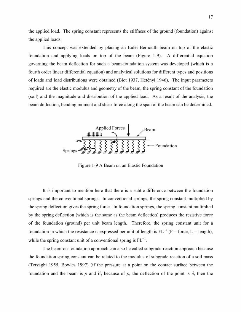
This concept was extended by placing an Euler-Bernoulli beam on top of the elastic
foundation and applying loads on top of the beam (Figure 1-9). A differential equation
governing the beam deflection for such a beam-foundation system was developed (which is a
fourth order linear differential equation) and analytical solutions for different types and positions
of loads and load distributions were obtained (Biot 1937, Hetényi 1946). The input parameters
required are the elastic modulus and geometry of the beam, the spring constant of the foundation
(soil) and the magnitude and distribution of the applied load. As a result of the analysis, the
beam deflection, bending moment and shear force along the span of the beam can be determined.
Applied Forces Beam
Foundation Springs
Figure 1-9 A Beam on an Elastic Foundation
It is important to mention here that there is a subtle difference between the foundation
springs and the conventional springs. In conventional springs, the spring constant multiplied by
the spring deflection gives the spring force. In foundation springs, the spring constant multiplied
by the spring deflection (which is the same as the beam deflection) produces the resistive force
of the foundation (ground) per unit beam length. Therefore, the spring constant unit for a
foundation in which the resistance is expressed per unit of length is FL−2 (F = force, L = length),
while the spring constant unit of a conventional spring is FL−1.
The beam-on-foundation approach can also be called subgrade-reaction approach because
the foundation spring constant can be related to the modulus of subgrade reaction of a soil mass
(Terzaghi 1955, Bowles 1997) (if the pressure at a point on the contact surface between the
foundation and the beam is p and if, because of p, the deflection of the point is δ, then the

18
modulus of subgrade reaction is given by p/δ and has a unit of FL−3). The modulus of subgrade
reaction multiplied by the width of the beam gives the foundation spring constant. In fact, the
spring constants are often estimated by determining the soil subgrade reaction modulus (the
modulus can be determined experimentally, e.g., by performing a plate load test).
The beam-on-foundation concept was adapted by the researchers on laterally loaded piles
(Davisson 1970, Francis 1964, Broms 1964a, b, Matlock and Reese 1960, Reese and Matlock
1956) because, in most cases, the piles behave as flexible beams against lateral (transverse) loads
and the problem can be looked upon as a beam-on-foundation problem rotated by 90° (Figure 1-
10). However, the laterally loaded pile problem is more complex because soils in real field
situations behave nonlinearly, particularly near the top part of the pile. In other words, because
of the nonlinear nature of a typical soil stress-strain plot, the head deflection of piles, when
plotted against applied load, produce a nonlinear curve. The linear springs, as hypothesized by
Winkler (1867), could no longer be used for laterally loaded piles, and were replaced by
nonlinear springs (for which the value of the spring constant changes with pile deflection). As a
result, the governing fourth order differential equation becomes nonlinear and the finite
difference method was used to iteratively solve the equation (McClelland and Focht 1958). In
order to simplify the problem, some researchers assumed the soil to be linear elastic up to a
certain value of pile deflection and perfectly plastic beyond that value (Bowles 1997, Hsiung and
Chen 1997).
Figure 1-10 A Laterally Loaded Pile in a Bed of Springs

19
Further modification of the beam-on-nonlinear-foundation approach led to the p-y
method (Matlock 1970, Reese et al. 1974, 1975, Reese and Welch 1975, Reese 1977, 1997,
O’neill et al. 1990). In the p-y method, p stands for the soil pressure (resistance) per unit pile
length and y stands for pile deflection (note that the soil resistance p is the product of pile
deflection and the nonlinear spring constant). Instead of giving inputs for the nonlinear spring
constant (i.e., the values of the spring constant as a function of pile deflection), p-y curves are
given as inputs to the analysis in the p-y method. Different p-y curves have been developed over
the years for different soil types, which give the magnitude of soil pressure as a function of the
pile deflection (Reese et al. 1974, 1975, Reese and Welch 1975, Matlock 1970, Georgiadis 1983,
O’Neill et al. 1990, Georgiadis et al. 1992, Yan and Bryne 1992, Gabr et al. 1994, Brown et al.
1994, Reese 1997, Wu et al. 1998, Bransby 1999, Zhang et al. 1999a, Ashour and Norris 2000).
For the analysis, the pile is divided into small segments, and for each segment, a p-y curve is
given as input. Depending on the magnitude of the deflection of a pile segment, the correct soil
resistance is calculated from the p-y curve iteratively (since deflections and soil pressures are
interdependent and since neither is known a priori, iterations are necessary to obtain their correct
values) and solutions to the nonlinear fourth order differential equation are obtained using the
finite difference method. With the development of the finite element method, analysis using
beam finite elements have replaced the finite difference method in many calculations involving
the subgrade-reaction approach or the p-y method (Stewart 2000, Hsiung and Chen 1997, Sogge
1981). Today, the p-y method is the most widely used method for calculating the response of
laterally loaded piles.
The p-y method is often used for the analysis of pile groups as well. However, in order to
use the standard p-y curves developed for single piles, the p values are reduced to take into
account the reduced resistance that a pile in a group offers due to pile interactions. The reduction
in the values of p is generally done by multiplying p of the single-pile case by a multiplier f,
which depends, among other factors, on the number of piles in a group and their relative
positions with respect to the pile in question (Salgado 2008). Different values and equations of
the multiplier f have been proposed by various authors and are available in the literature (Brown
et al. 1991, McVay et al. 1998, Mokwa 1999, Ilyas et al. 2004, Reese et al. 2006).
Using the p-y method or the subgrade-reaction approach, pile deflection is estimated as a
function of applied load under working load conditions. In other words, design against the

20
serviceability limit state of tolerable lateral deflection can be done using the p-y method. Since
the serviceability limit state is the primary concern in the design of laterally loaded piles, the p-y
method has gained huge popularity, particularly in the US. Over the years, several modifications
and extensions of the beam-on-foundation approach and the p-y method have been made (Reddy
and Valsangkar 1970, 1971, Madhav et al. 1971, Scott 1981, Aköz et al. 1981, Hsiung 2003,
Shen and Teh 2004, Hsiung et al. 2006, Yang and Liang 2006). The characteristic load method
of Duncan et al. (1994), in which dimensionless equations are developed from p-y analysis, and
the strain wedge model of Ashour and Norris (2000), which considers a mobilized passive soil
wedge in front of the pile to determine p-y curves, are examples of these methods.
The ultimate capacity due to the structural failure of a pile can be determined by using the
p-y method if the plastic moment of the pile section is given as input to the p-y analysis.
However, the p-y method cannot model the slip mechanism that would form if zones of soil
adjacent to the pile were to yield. The beam-on-foundation approach can be used to calculate the
ultimate capacity due to soil yielding, in which the soil is assumed to be perfectly plastic and
limit soil resistance is used to estimate the ultimate lateral capacity. In such an approach, a limit
soil pressure (i.e., passive pressure) is assumed to act throughout the length of the pile (in one
direction above a certain center of rotation and in the opposite direction below it). The
magnitude of the limit soil pressure is estimated, the positions of plastic hinge formation in the
pile are located (required only for flexible piles), and force and moment equilibrium conditions
are applied to calculate the ultimate (limit) load and moment that can act at the pile head (Broms
1964a, b, Poulos and Davis 1980, Fleming et al. 1992, Zhang et al. 2005).
1.5.2. Continuum Approach
Analysis of laterally loaded piles can be done by treating the soil surrounding the pile as a
three-dimensional continuum. Such an approach is conceptually more appealing than the beam-
on-foundation approach because the interaction of the pile and the soil is indeed three-
dimensional in nature. Research in this direction was pioneered by Poulos (1971a), who treated
the soil mass as an elastic continuum and the pile as a strip, which applied pressure on the
continuum. He used Mindlin’s solution (Mindlin 1936) for horizontal load acting at the interior
of an elastic half space and applied a boundary integral technique to obtain pile deflection.

21
However, the method is less popular than the p-y method, most likely because the analysis steps
are relatively involved. The elastic analysis was extended to account for soil nonlinearity in an
approximate way by assuming elastic-perfectly plastic soil (Poulos 1972, 1973, Davies and
Budhu 1986, Budhu and Davies 1988). A similar boundary element analysis was performed by
Banerjee and Davies (1978).
Today, the most versatile continuum-based method of analysis available is the finite
element method. The method can take into account the three-dimensional interaction, and both
elastic and nonlinear soils can be simulated by giving inputs of elastic constants (e.g., Young’s
modulus and Poisson’s ratio) or by plugging in appropriate nonlinear constitutive relationships.
Several researchers have used different forms of the finite element method (e.g., two-
dimensional analysis, three-dimensional analysis, finite elements coupled with Fourier
techniques, finite elements coupled with finite difference, finite elements with substructuring) to
analyze laterally loaded piles (Desai and Appel 1976, Randolph 1981, Kooijman and Vermeer
1988, Verruijt and Kooijman 1989, Trochanis et al. 1991, Bhowmik and Long 1991, Bransby
1999).
Other continuum-based analysis methods are also available (Baguelin et al. 1977, Pyke
and Beikae 1984, Lee et al. 1987, Lee and Small 1991, Sun 1994a, Guo and Lee 2001, Einav
2005). However, these methods are rarely used by practitioners because either the analyses
involve complicated mathematics and do not provide simple, practical steps for obtaining pile
deflection or the methods are applicable only to linear elastic soils, which do not represent the
reality of practical problems.
Continuum-based analyses have also been used to analyze pile groups. The boundary
integral technique was used to capture the interaction between piles in groups (Poulos 1971b,
Banerjee and Davies 1980, Basile 1999, Xu and Poulos 2000). The finite element method
(Shibata et al. 1988, Chow 1987) and variational methods (Shen and Teh 2002) have been
applied to pile-group problems as well. Because of the difficulties of applying the finite element
method to large pile groups, Law and Lam (2001) proposed the application of periodic boundary
conditions in finite element analysis of large pile groups. Additionally, some hybrid methods
coupling both the continuum approach and the p-y have been used to model pile groups (Foch
and Koch 1973, O’Neil et al. 1977, Horsnell et al. 1990).

22
1.6. Motivation for this Research Work
The beam-on-foundation approach or the p-y method is an ideal candidate for laterally
loaded-pile analysis from a practical point of view because of the ease with which solutions can
be obtained. Solutions of the ordinary fourth order differential equation, even if nonlinear, can
be obtained quickly. The assumption of an Euler-Bernoulli beam for the pile is satisfactory
because most flexible piles are slender enough so that shear stresses and deformations within the
piles can be neglected. However, springs are a poor representation of the surrounding soil. The
interaction of a laterally loaded pile with the soil is three-dimensional in nature; the resistive
properties of each element of soil surrounding the pile add up to generate the overall resistance
against pile movement. Therefore, the nonlinear spring constant should be related to the resistive
properties (e.g., stress-strain response) of the soil elements by taking into account the three-
dimensional interaction. Unfortunately, such a rigorous relationship is not available; for the
beam-on-foundation approach, the spring constants are mostly estimated from empirical or semi-
empirical correlations (Francis 1964, Poulos and Davis 1980, Scott 1981, Bowles 1997, Hsiung
and Chen 1997, Ashford and Juirnarongrit 2003).
The same limitation is applicable for the p-y curves as well. The method of preparation
of the p-y curves developed from field observation and experience (Matlock 1970, Reese et al.
1974, 1975). The p-y curves used today are mostly obtained either by back fitting the results of
numerical analysis (of the fourth-order beam-on-foundation equation) to match the observed
deflections in the field or the results of model tests; or by correlating the curves with soil
properties determined by laboratory or in-situ tests; or by comparing the results of p-y analysis
with other numerical analyses (Matlock 1970, Reese et al. 1974, 1975, Brown and Kumar 1989,
Yan and Byrne 1992, Brown et al. 1994, Gabr et al. 1994, Briaud 1997, Wu et al. 1998, Bransby
1999, Ashour and Norris 2000, Anderson et al. 2003). As a result, the p-y curves are site-
specific and do not take into account the three-dimensional pile-soil interaction. Considerable
judgment is required for using the p-y curves to predict proper pile response; in fact, analyses
using the standard p-y curves often are reported to have failed to predict the actual pile load-
deflection response (Yan and Byrne 1992, Anderson et al. 2003, Kim et al. 2004). For example,
Figure 1-11 (adapted from Kim et al. 2004) compares the p-y curves obtained from back
calculation of the results of model tests on steel piles installed in Nak-Dong river sand, as
reported by Kim et al. (2004), with the standard p-y curves for sands proposed by Reese et al.

23
(1974), O’Neill and Murchinson (1983) and Wesselink et al. (1988) that are used in design. The
figure clearly shows the deficiency of the standard p-y curves in producing reliable designs.
Reese et al. (1974)
O’Neill and Murchinson (1983)
Wesselink et al. (1988)
Driven Pile
Pre-installed Pile
0 0.05 0.1 0.15 0.2 0.25
0.8
0.6
0.4
0.2
0.0
y/D
p (k
N/m
)
Reese et al. (1974)
O’Neill and Murchinson (1983)
Wesselink et al. (1988)
Driven Pile
Pre-installed Pile
Reese et al. (1974)
O’Neill and Murchinson (1983)
Wesselink et al. (1988)
Driven Pile
Pre-installed Pile
0 0.05 0.1 0.15 0.2 0.25
0.8
0.6
0.4
0.2
0.0
y/D
p (k
N/m
)
Figure 1-11 Comparison of Pile Resistance p versus Normalized Pile Deflection y/D (D is the Pile Diameter) Curves Obtained from Model Tests with the Standard Curves Available for
Design (Adapted from Kim et al. 2004)
The finite element method, in its three-dimensional form, has the potential for producing
realistic results for laterally loaded piles if appropriate soil constitutive relationships are used and
if appropriate elements and domains are chosen for the soil and the pile. However, the enormous
computation time and resources required for such an analysis prohibit practitioners from using
finite elements in routine design.
An ideal method of analysis should have the rigor of a three-dimensional continuum
approach, but should produce results as quickly as the beam-on-foundation approach. This is
precisely the aim of this research. We hypothesize that a continuum-based, three-dimensional
analysis can be developed for laterally loaded piles that rigorously relates the overall resistance
of a soil mass to the soil constitutive relationship (i.e., stress-strain relationship). The analysis
would take into account the actual pile-soil interaction and add up the resistances of each soil
element to produce the total soil resistance. Consequently, the nonlinear properties of soil would
be explicitly used to produce the nonlinear pile response, and the p-y curves would no longer be

24
required. We further envisage connecting the continuum-based analysis to the to the beam-on-
foundation approach so that the ordinary differential equation of the beam-on-foundation
approach can be used to quickly obtain pile deflection. A particular aim is to develop the
solutions in closed form so that expensive computer resources, essential for numerical analyses
(e.g., by using finite elements), can be avoided.
1.7. Scope of Present Study
We develop a method of analysis of a laterally loaded pile embedded in a multi-layered
soil medium and subjected to a horizontal force and moment at the pile head. Only static
response is considered. We focus on serviceability and settlement-based limit states; i.e., we
develop an analysis by which pile deflections can be predicted for the initial stages of loading
(typically, a maximum pile-head deflection of the order of 25 mm is used as the criterion for
serviceability limit state). The research starts with the development of a general framework,
which shows logically how an improved beam-on-foundation model can be used to effectively
analyze a laterally loaded pile embedded in a multi-layered soil. Then a continuum-based
analysis is performed, which rigorously connects the properties of the three-dimensional
continuum surrounding the pile to those of the soil springs, so that a one-to-one correspondence
between the continuum-based approach and the beam-on-foundation approach can be established.
The analysis is subsequently improved to incorporate the nonlinear stress-strain relationships of
soils in the model. Finally, a method for pile group analysis of is presented.
In chapter 2, the pile is modeled as a beam resting on a multi-layered elastic foundation
and solution for pile deflection is obtained analytically by using the method of initial parameters.
In chapter 3, an elastic continuum model is introduced which is subsequently modified to
incorporate soil nonlinearity in chapter 4. In chapter 5, we extend the analysis to pile groups.
Finally, in chapter 6, we consolidate the research findings and propose future extensions of the
research.

25
CHAPTER 2. LATERALLY LOADED PILE IN LAYERED ELASTIC MEDIUM: A BEAM-ON-ELASTIC-FOUNDATION APPROACH
2.1. Introduction
In this chapter, we derive the governing differential equations for deflection of laterally
loaded piles using a beam-on-elastic-foundation approach. Such an approach illustrates how
simple idealizations of the statics and kinematics of pile-soil interaction can be used to model a
laterally loaded pile as a beam resting on a foundation comprising of a series of springs. We
derive the equations for multi-layered, elastic foundations. Then we obtain the analytical
solutions for pile deflection, slope of the deflected curve (elastic curve), bending moment and
shear force within each layer by using the method of initial parameters. Finally we discuss the
modifications of the analytical solutions required for applying the solutions to long piles.
2.2. Overview
The beam-on-foundation model has been used in the past to analyze the response of
laterally loaded piles (Broms 1964a, b, Matlock and Reese 1960, Fleming et al. 1992, Bowles
1997). Generally, a one-parameter foundation model represented by k is considered (k being the
spring constant per unit pile/beam length), although a two parameter model (which includes the
shear parameter t in addition to k) can also be used.
In order to account for soil nonlinearity, modification of the linear one-parameter model
has been done by replacing the linear Winkler springs with nonlinear springs (McClelland and
Focht 1958). For nonlinear springs, the spring constant k (per unit pile or beam length) depends
on the pile (beam) deflection w (in general, the value of k decreases with increasing w). Hence,
the soil reaction per unit length p = kw does not increase linearly with w. The nonlinear
modification of the one-parameter model culminated in the development of the p-y method
(Reese and Cox 1969, Matlock 1970, Reese et al. 1974, 1975, Reese and Van Impe 2001). In the
p-y method, k is no longer given as input (as a function of w); the nonlinear relationship of k (or
26
p) with w are given as inputs to the analysis in the form of p-w curves, which are widely known
in the literature as “p-y” curves.
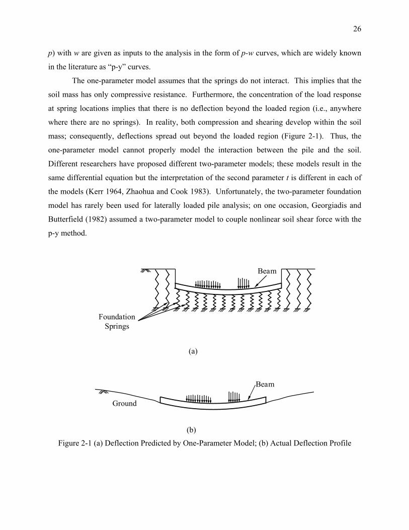
The one-parameter model assumes that the springs do not interact. This implies that the
soil mass has only compressive resistance. Furthermore, the concentration of the load response
at spring locations implies that there is no deflection beyond the loaded region (i.e., anywhere
where there are no springs). In reality, both compression and shearing develop within the soil
mass; consequently, deflections spread out beyond the loaded region (Figure 2-1). Thus, the
one-parameter model cannot properly model the interaction between the pile and the soil.
Different researchers have proposed different two-parameter models; these models result in the
same differential equation but the interpretation of the second parameter t is different in each of
the models (Kerr 1964, Zhaohua and Cook 1983). Unfortunately, the two-parameter foundation
model has rarely been used for laterally loaded pile analysis; on one occasion, Georgiadis and
Butterfield (1982) assumed a two-parameter model to couple nonlinear soil shear force with the
p-y method.
Beam
Foundation Springs
(a)
Beam
Ground
(b)
Figure 2-1 (a) Deflection Predicted by One-Parameter Model; (b) Actual Deflection Profile

27
Another analysis approach is available in which the pile is treated as an Euler-Bernoulli
beam and the surrounding soil mass is treated as an elastic continuum with a simplified
assumption on the displacement field (Sun 1994a, Guo and Lee 2001). The analysis finally
produces equations that are the same as the two-parameter-model equations. Thus, all these
(one-parameter, two-parameter or continuum) approaches finally result in similar fourth-order
differential equations, with pile deflection w as the variable.
If the soil is assumed to be linear elastic, then the differential equations are also linear,
and closed-form solutions for pile deflection can be obtained by solving the differential
equations with proper boundary conditions. In the case of nonlinear soils, the equations are
nonlinear, and numerical methods like the finite element method or the finite difference method
are generally used to solve the problem. This applies equally to the continuum approach and to
the p-y method, which is formulated using nonlinear (p-y) springs (McClelland and Focht 1958,
Stewart 2000). For linear soils, general solutions of the fourth-order, linear differential equations
are readily available (Hetényi 1946, Vlasov and Leont’ev 1966), and the four constants of
integration can be determined from the pile boundary conditions (Sun 1994a, Guo and Lee
2001).
Soil layering is an important factor that affects laterally loaded pile response (Basu and
Salgado 2007a). Layering has been taken into account approximately in some pile analyses by
either assuming (typically) a linear variation of k with depth or by proposing different p-y curves
for different soil depths (Broms 1965, Matlock and Reese 1960, Davisson 1970, Madhav et al.
1971, Valsangkar et al. 1973, Scott 1981, Ashour et al. 1998, Hsiung 2003). Such gradual
variation of soil properties with depth has been assumed in many continuum-based analyses as
well (Poulos 1973, Randolph 1981, Budhu and Davies 1988, Zhang et al. 2000, Banerjee and
Davies 1978). However, in real field situations, discrete soil layers are often present and the
assumption of linear (or similar) variation of soil properties does not properly represent the
ground conditions. Analyses considering explicit layering (i.e., with multiple layers) are rather
limited. Davisson and Gill (1963) analyzed a two-layer system using the p-y method.
Georgiadis (1983) developed a method of developing p-y curves for layered soil profiles. A few
continuum-based numerical analyses are also available (Pise 1982, Lee et al. 1987, Veruijt and
Kooijman1989). Thus, in order to design laterally loaded piles for practical problems, a method
of analysis by considering a multi-layered deposit needs to be developed.

28
Although closed-form solutions of the fourth-order differential equation governing
laterally loaded pile deflection exist for linear-elastic, homogeneous soils (Sun 1994a, Guo and
Lee 2001), algebraic solutions for piles embedded in multi-layered soil deposits are difficult to
obtain (albeit theoretically possible) because of the increased number of constants of integration.
For example, for a four-layer laterally loaded pile problem, there are sixteen constants of
integration (four constants per layer) that need to be determined algebraically by solving a set of
sixteen simultaneous equations, arising due to the boundary conditions.
A finite element analysis using beam elements or a finite difference analysis can be used
to analyze the problem (Scott 1981, Zhaohua and Cook, 1983, Sun 1994b). However, as
described in chapter 3, our analysis requires the calculation of integrals, along depth, of the
square of pile defection and slope. These integrations are performed numerically and require
fine discretization of the pile along its length for accurate results. Therefore, if finite element or
finite difference methods are used, the number of discretized pile elements will have to be very
large resulting in increased computation time. Thus, obtaining analytical solutions of the pile-
deflection equation is necessary for our analysis.
We obtain analytical solutions by using the method of initial parameters (MIP), also
known as the method of initial conditions (Hetényi 1946, Vlasov and Leont’ev 1966, Selvadurai
1979, Basu and Salgado 2007b), which yields the final analytical solutions without directly
determining the integration constants. MIP was originally developed for solving problems of
beams on elastic foundations (Hetényi 1946, Vlasov and Leont’ev 1966, Harr et al. 1969, Rao et
al. 1971). The method is particularly useful when some form of discontinuity exists within the
span of a beam. MIP has been applied to problems where the discontinuity is caused due to the
application of concentrated forces at different points along the span of a beam (Vlasov and
Leont’ev 1966, Harr et al. 1969, Rao et al. 1971).
In this chapter, we develop the equations for pile deflection following the beam-on-
elastic-foundation approach by considering both the one-parameter and two-parameter
foundation models. This helps us to distinguish between the two models and to identify the
advantages of the two-parameter model over the one-parameter model. We then modify the
existing MIP to account for discontinuities along a pile caused by abrupt change in soil
properties due to soil layering. This allows us to obtain analytical solutions for deflection of
laterally loaded piles embedded in multi-layered elastic soils. We do not address the issue of soil

29
nonlinearity in this chapter. However, the framework built in this chapter is subsequently
improved in chapter 3 by incorporating a rigorous, continuum-based analysis, which culminates
in the incorporation of soil nonlinearity in chapter 4.
2.3. Problem Definition
We consider a pile of constant flexural rigidity EpIp (Ep is the Young’s modulus of the
pile and Ip is the second moment of inertia of the pile section) and length Lp embedded in a
multi-layered soil deposit (Figure 2-2). The soil is assumed to behave as a linear, elastic
material. There are n horizontal soil layers, with the bottom (nth) layer extending to infinity
downward. The vertical depth to the bottom surface of any intermediate layer i is Hi, which
implies that the thickness of layer i is Hi − Hi−1 with H0 = 0. The pile top (head) is at the level of
the ground surface. The bottom (base) of the pile is considered embedded in the nth layer. The
pile is acted upon by a horizontal force Fa and moment Ma at the pile head.
We assume a right-handed Cartesian coordinate system x-y-z with its origin at the center
of the pile head such that the z axis coincides with the pile axis and the x-z plane coincides with
the plane of the paper. The force Fa acts in the x direction and lies on the x-z plane. The moment
Ma, when expressed as a vector following the right-hand cork screw rule, acts into the plane of
the paper (i.e. opposite y-direction). The bending of the pile takes place in the x-z plane.
2.4. Differential Equation and Boundary Conditions
The pile is modeled as an Euler-Bernoulli beam. Considering the equilibrium of a pile
cross section, as it bends under the action of the applied loads (Figure 2-3), we arrive at:
np
MxI
σ = (2-1)
where σn is the normal stress within the pile in the direction of the pile axis (i.e., z-axis); x
is the distance of the point (from the pile cross-section neutral axis) at which the normal stress σn
acts; M = M(z) is the bending moment acting at the cross section (the positive sign convention
for M is shown in Figure 2-4). The corresponding normal strain (assuming compression
positive) in the pile cross section can be obtained from equation (2-1) as:

30
Hn-2
Hi
Hi-1
H2
xMa
…
…
…
…
Hn-1
H1 Layer 1
Layer 2
Layer i
Layer n−1
Layer n
z
Fa
Pile
Lp
∞
y
xFa
MaPile
Figure 2-2 (a) A Laterally Loaded Pile in a Layered Soil Medium
np p
MxE I
ε = (2-2)
Considering the kinematics of the pile, we develop the following equation: 2
2i nd w
dz xε
= (2-3)
where wi = wi(z) is the lateral pile deflection at a depth z (at a level corresponding to the
ith layer) from the pile head.
Combining the statics and kinematics, we get (for the ith layer): 2
2i
p p id wE I Mdz
= (2-4)
As we go down the pile by an infinitesimal distance dz, the shear force Sp = Sp(z) on the
pile cross section increases by dSp (the positive sign convention for Sp is shown in Figure 2-4).

31
Since the surrounding soil mass offers resistance to pile movement (Figure 2-3), the rate at which
the shear force in the pile section increases over an infinitesimal length dz can be related to the
soil resistance p = p(z) (produced by a “soil column” (Figure 2-3) of infinitesimal thickness dz)
acting on the element (Figure 2-4).
dz
Pile element of infinitesimal
length dz
w(z)
“Soil column” of infinitesimal thickness dz providing resistance to pile movement
Soil columns get compressed (spring effect) due to pile movement from, say, point A to point B
B
Pile (undeformed
configuration) …
Ground Surface
Pile (deformed configuration)
…
A
Shear resistance develops between soil columns due to differential lateral movement
z
Figure 2-3 Pile-Soil Interaction
The soil resistance p is a continuous, distributed force (per unit length) acting along the
pile shaft in the negative w(z) direction. The total soil resistance p against pile movement has
contributions from both the soil compressive resistance pc (since, the soil columns are
compressed as the pile presses against them) and the soil shear resistance ps (since, the soil
columns slide relative to each other due to differential change in pile deflection with depth)
(Figure 2-3). Thus, for any layer i, we get (Figure 2-5):
i ci sip p p= + (2-5)

32
w(z)
z
M
Sp and Ss
γs
θ = dwdz
Positive Sign Convention
Figure 2-4 Sign Conventions Used
pM
M + dM
p
Pile element
Sp(z)
Sp + dSp
Ss(z)
Ss + dSs
pc
Soil column or spring
= pc
Ss + dSs
pc
Ss(z)
ps
+
dz
dz
Figure 2-5 Equilibrium of Pile and Soil
The total soil resistance p balances the change in pile shear force dSp over an infinitesimal
length dz and keeps the pile element in equilibrium (Figure 2-5). Therefore, considering the

33
force equilibrium of the pile element for the ith layer, we get ( ) 0pi pi pi iS S dS p dz− + − = , which
gives:
pi idS p dz= − (2-6)
The increase dMi in the bending moment over the infinitesimal distance dz can be related
to the shear force Spi using moment equilibrium of the pile element (Figure 2-5) as
( ) 02i i pi idzM M dM S dz p dz− + + − + = . Neglecting the higher order term we get:
i pidM S dz= (2-7)
Equations (2-6) and (2-7) yield:
pii
dSp
dz= − (2-8)
and
ipi
dM Sdz
= (2-9)
Using equations (2-8) and (2-9), equation (2-4) can be rewritten as: 4
4i
p p id wE I pdz
= − (2-10)
Let us now consider the equilibrium of a soil column of infinitesimal thickness dz at a
depth z as shown in Figure 2-5. As mentioned before, the soil resistance pc develops because of
the compressive resistance of the soil column. Thus, in order to model the compressive
resistance, the soil column can be replaced by an equivalent “soil spring” that reproduces the
same compressive resistance. Consequently the part pc of the soil resistance in the ith layer can
be expressed as:
ci i ip k w= (2-11)
where ki is the spring constant (FL−2).
The soil columns move by different amounts as the pile deflects and bends in order to
maintain displacement compatibility (Figure 2-3). Since soil offers resistance against shearing,
shear forces are developed at the interfaces of adjacent soil columns due to their relative motion.
The relative motion is not a constant with depth because the pile slope θ ( )dw dz= (i.e., the rate
at which the pile deflection changes from one depth to another) is not a constant. Consequently,

34
the soil shear force Ss = Ss(z) is a function of z. As we move by an infinitesimal distance dz, the
soil shear force increases from Ss to Ss + dSs (the positive sign convention of Ss is given in Figure
2-4). The change in the soil shear force dSs over a distance dz is balanced by the soil resistance
ps (Figure 2-5). Thus, considering the equilibrium of a soil element in the ith layer we get
( ) 0si si si sip dz S S dS+ − + = , which, along with equation (2-5) gives:
( ) ( )si si i ci i i idS p dz p p dz p k w dz= = − = − (2-12)
The average soil shear stress arising from the soil shear force Ssi can be related to the
corresponding engineering shear strain γs as:
12
si sis
si e i
S SG A t
γ = = (2-13)
where Gsi is the average soil shear modulus in the ith layer; Ae is an equivalent area in the soil that
relates the soil shear force to the corresponding average soil shear stress; and ti is the soil shear
parameter, which is related to the soil shear modulus (ti has a unit of force). The engineering
shear strain γs is also equal to the negative of the pile slope ii
dwdz
θ = (a positive shear strain in
the soil column causes a negative pile slope because of the sign convention for soil shear force
shown in Figure 2-3). Therefore, from equation (2-13), we get:
2 isi i
dwS tdz
= − (2-14)
Using equations (2-12) and (2-14) we get: 2
22 ii i i i ci si
d wp k w t p pdz
= − = + (2-15)
The above equation also follows from the continuum model, as will be seen in chapter 3, if some
simplifying assumptions regarding the soil displacement fields are made.
In the case of the one-parameter model, the shear resistance of soil is neglected (i.e., ti =
0, which means psi = 0). Consequently, using equations (2-10) and (2-15) with psi = 0, we get: 4
4 0ip p i i
d wE I k wdz
+ = (2-16a)
In the case of the two-parameter model or the continuum model, in which the soil shearing
resistance is taken into account, we get from equations (2-10) and (2-15):

35
4 2
4 22 0i ip p i i i
d w d wE I t k wdz dz
− + = (2-17a)
Equations (2-16a) and (2-17a) are the governing differential equations for pile deflection
considering the one-parameter and the two-parameter (or the continuum) models, respectively.
The bending moment at any pile section at a depth z is expressed in terms of pile
deflection in equation (2-4). The shear force on any horizontal plane (which passes through both
the pile and the soil) at any depth is the sum of the shear force Sp acting in the pile section and
the shear force Ss acting in the soil. The shear force Sp in the pile section can be expressed in
terms of pile deflection using equations (2-4) and (2-7) as:
3
3i i
pi p pdM d wS E Idz dz
= = (2-18)
The soil shear force Ss is expressed in terms of pile deflection in equation (2-14). Hence,
the total shear force S at any depth z within the ith layer can be expressed as:
dzdwt
dzwdIESSS i
ii
ppsipii 23
3
−=+= (2-19)
In the case of the one-parameter model, Ssi in the above equation is equal to zero (ti = 0); thus,
the one-parameter model does not take into account the shear resistance of soil. The soil
resistance pi is given by equation (2-11) for the one-parameter model and by equation (2-15) for
the two-parameter (or continuum) model.
In an Euler-Bernoulli beam, the deflection, slope, bending moment and shear force is
continuous along its span. In order to satisfy equilibrium at the beam ends (boundaries), any
applied concentrated force (or reaction force) at the ends must be equal to the shear force at the
corresponding sections (or the negative of the shear force, depending on the choice of sign
convention). Similarly, any applied concentrated moment (or moment generated as a reaction
due to restraints in rotation) at the ends must be equal to the bending moment at the
corresponding sections (or the negative of the bending moment, depending on the choice of sign
convention). In the case of laterally loaded piles, this is also true. These continuity and
equilibrium requirements produce the boundary conditions for the governing differential
equations (2-16a) and (2-17a).
For our problem, the boundary conditions for equations (2-16a) and (2-17a) at the pile
head (z = 0) are:

36
31 1
130
2p p a
z
d w dwE I t Fdz dz
=
⎡ ⎤− =⎢ ⎥
⎣ ⎦ (2-20a)
and
1
0
0z
dwdz =
= (2-21a)
or 2
12
0p p a
z
d wE I Mdz
=
= (2-22a)
At the interface between the ith and (i + 1)th layer (i.e., at z = Hi), the boundary conditions
are:
1i i
i iz H z Hw w += =
= (2-23a)
1
i i
i i
z H z H
dw dwdz dz
+
= =
= (2-24a)
2 21
2 2
i i
i i
z H z H
d w d wdz dz
+
= =
= (2-25a)
3 31 1
13 32 2i i
i i i ip p i p p i
z H z H
d w dw d w dwE I t E I tdz dz dz dz
+ ++
= =
⎡ ⎤ ⎡ ⎤− = −⎢ ⎥ ⎢ ⎥
⎣ ⎦ ⎣ ⎦ (2-26a)
At the pile base (z = Lp) the boundary conditions are:
0p
n z Lw
== (2-27a)
or 3
13 2 2p
p
n np p n n n n z L
z L
d w dwE I t k t wdz dz + =
=
⎡ ⎤− =⎢ ⎥
⎣ ⎦ (2-28a)
and
0p
n
z L
dwdz =
= (2-29a)
or 2
2 0p
n
z L
d wdz
=
= (2-30a)

37
with ti = 0 for the one-parameter model.
Equation (2-20a) states that, at the pile head, the shear force is equal to the applied
horizontal force. The direction of the applied force Fa produces a positive shear force at the pile
head. For two-parameter models, the shear force in the pile section and the shear force in the soil
have to be considered together. Equations (2-21a) and (2-22a) state that at the pile head either
the slope is equal to zero (this is the fixed-head condition, which might occur if a pile cap is
present that may be considered to completely restrain pile head rotation) or the bending moment
is equal to the applied moment (this is the free-head condition, which occurs when there is no
pile cap present and the pile head is free to rotate). The direction of the applied moment Ma
produces a positive bending moment at the pile head. Equations (2-23a) through (2-26a) ensure
the continuity of the deflection, slope, bending moment and shear force across adjacent layers.
Equations (2-27a) and (2-28a) state that, at the pile base, either the deflection is equal to zero
(this is the fixed-base condition, which may be assumed to occur when the pile is socketed into a
very firm layer, like rock) or the shear force just above the base of the pile is equal to the shear
force just below the base. It is worth mentioning here that, for the two-parameter or the
continuum model, the shear force just below the pile base is equal to 12p
n n n z Lk t w+ =
(equation
(2-28a)) as will be seen in chapter 3 (tn+1, defined in chapter 3, quantifies the shear force at the
pile base produced by the soil column that starts immediately below the pile and extends to
infinity downward and has the same cross section as the pile). For the one-parameter model (ti =
0), the shear force just below the pile base is equal to zero (which does not represent the real
field condition and is a limitation of the one-parameter model). Equations (2-29a) and (2-30a)
state that, at the pile base, either the slope is zero (valid for fixed-base condition) or the bending
moment is zero (this is the free-base condition which might occur if the pile base floats in a soft
layer of soil).
Equations (2-16a) and (2-17a) are normalized with respect to the length Lp of the pile so
that the results are applicable to any field conditions. We accomplished this by introducing the
dimensionless variables z = z/Lp and w = w/Lp (note that pdz dz L= ). The relationships of the
successive differentiations of the normalized deflection function w(z ) with respect to the
normalized space (independent) variable z with those of the original variables with dimensions
are given by:

38
1p
p p
dw d w dz dw dwLdz dz L dz L dz dz
⎛ ⎞= = =⎜ ⎟⎜ ⎟
⎝ ⎠ (2-31a)
2 2
2 2p pd w d dw dz d dw d wL Ldz dz dz dz dz dz dz
⎛ ⎞ ⎛ ⎞= = =⎜ ⎟ ⎜ ⎟⎝ ⎠ ⎝ ⎠
(2-31b)
3 2 2 32
3 2 2 3p p pd w d d w dz d d w d wL L Ldz dz dz dz dz dz dz
⎛ ⎞ ⎛ ⎞= = =⎜ ⎟ ⎜ ⎟
⎝ ⎠ ⎝ ⎠ (2-31c)
4 3 3 42 3
4 3 3 4p p pd w d d w dz d d w d wL L Ldz dz dz dz dz dz dz
⎛ ⎞ ⎛ ⎞= = =⎜ ⎟ ⎜ ⎟
⎝ ⎠ ⎝ ⎠ (2-31d)
Using the above relationships in equations (2-16a) and (2-17a), we get the normalized
form of the governing differential equations for the one-parameter and the two-parameter (or
continuum) models as: 4
4 0ii i
d w k wdz
+ = (2-16b)
4 2
4 22 0i ii i i
d w d wt k wdz dz
− + = (2-17b)
where 4
i pi
p p
k Lk
E I= (2-32)
2i p
ip p
t Lt
E I= (2-33)
The slope ii
dwdz
θ = , bending moment Mi (equation (2-4)), shear force Si (equation 2-19)
and soil resistance pi (equation (2-15)) (in the ith layer) are respectively normalized and
expressed in terms of the normalized pile deflection wi using the relationships given by equations
(2-31a) through (2-31c) as:
zdwd i
i ~~~
=θ (2-34)
2
2
~~~
zdwd
IELM
M i
pp
pii == (2-35)

39
zdwdt
zdwd
IELS
S ii
i
pp
pii ~
~~2~~~3
32
−== (2-36)
3 2
22i p ii i i i
p p
p L d wp k w tE I dz
= = − (2-37)
The applied force and moment can be similarly normalized as:
pp
paa IE
LFF
2~ = (2-38)
pp
paa IE
LMM =~ (2-39)
The normalized boundary conditions for equations (2-16b) and (2-17b) at the pile head (z
= 0) are: 3
1 113
0
2 a
z
d w dwt Fdz dz
=
⎡ ⎤− =⎢ ⎥
⎣ ⎦ (2-20b)
and
1
0
0z
dwdz =
= (2-21b)
or 2
12
0a
z
d w Mdz
=
= (2-22b)
At the interface between the ith and (i + 1)th layer (i.e., at z = Hi; where Hi = Hi/Lp), the
boundary conditions are:
1i i
i iz H z Hw w += =
= (2-23b)
1
i i
i i
z H z H
dw dwdz dz
+
= =
= (2-24b)
2 21
2 2
i i
i i
z H z H
d w d wdz dz
+
= =
= (2-25b)
3 31 1
13 32 2i i
i i i ii i
z H z H
d w dw d w dwt tdz dz dz dz
+ ++
= =
⎡ ⎤ ⎡ ⎤− = −⎢ ⎥ ⎢ ⎥
⎣ ⎦ ⎣ ⎦ (2-26b)
At the pile base (z = 1) the boundary conditions are:

40
10n z
w== (2-27b)
or 3
13 11
2 2n nn n n n z
z
d w dwt k t wdz dz + =
=
⎡ ⎤− =⎢ ⎥
⎣ ⎦ (2-28b)
and
1
0n
z
dwdz =
= (2-29b)
or 2
21
0n
z
d wdz
=
= (2-30b)
with ti = 0 for the one-parameter model. Note that the normalized shear force at the pile
base, for the two-parameter or the continuum model, is equal to 1 12 n n n z
k t w+ = (equation (2-
28b)) as we will show in chapter 3.
2.5. General Solutions
The general solution for both equations (2-16b) and (2-17b) is:
4)(
43)(
32)(
21)(
1)~(~ Φ+Φ+Φ+Φ= iiiii CCCCzw (2-40)
where, ( )1
iC , ( )2
iC , ( )3
iC and ( )4
iC are integration constants for the ith layer; and Φ1, Φ2, Φ3 and Φ4
are functions of z that are individual solutions of the differential equation (2-16b) or (2-17b).
The above general solution is not valid for long piles; we discuss the solution procedure for long
piles later in the chapter.
Assuming a general solution of the form ( ) mzw z e= , the auxiliary equation corresponding
to equation (2-16b) is given by: 4 0im k+ = (2-41)
Solution of equation (2-41) produces 2im k= ± − . Introducing the imaginary unit i with
the property i2 = − 1, we can write 2im i k= ± , which produces im i k= ± ± . Therefore, m

41
can be expressed as a complex number of the form m a ib= + , which yields
2 2 2 2 im a b abi i k= − + = ± . Since the real and imaginary part of a complex number are
independent of each other, we get 2 2 0a b− = and 2 iab k= ± . These two equations, when
solved simultaneously, produce 4 4ia b k= ± = ± . Thus, we get
( ) ( ) ( ) ( ){ }4( ) cos sin cos 4 sin 4 .ik za ib zmz az ibz az
i iw z e e e e e bz i bz e k z i k z±+= = = = + = ± + ± The
four possible combinations of signs of a and b produce the functions Φ1, Φ2, Φ3 and Φ4 (which
are individual solutions of equation (2-16b)) as combinations of trigonometric and exponential
(or hyperbolic) functions as given in Table 2-1.
The auxiliary equation corresponding to equation (2-17b) is 4 22 0i im t m k− + = (2-42)
Solution of equation (2-42) produces 2i i im t t k= ± ± − , which leads to three
conditions: 1) ki > ti2, 2) ki < ti2 and 3) ki = ti2. Since condition 3) can occur only under very
special conditions (when the numerical value of the square of ki exactly equals the numerical
value of ti), we deal with the first two conditions only. Condition 1) makes m a complex number
of the form m a ib= + , similar to the case of equation (2-41), so that
2 2 2 22 i i im a b abi t i k t= − + = ± − , which yields 2 2ia b t− = and 22 i iab k t= − . Solving these
two equations simultaneously gives the expressions for a and b, which are given in Table 2-1.
Since m is complex, Φ1, Φ2, Φ3 and Φ4 are again combinations of trigonometric and hyperbolic
functions. To satisfy condition 2), m does not require an imaginary part; consequently, Φ1, Φ2,
Φ3 and Φ4 are exponential or hyperbolic functions. Table 2-1 gives the detailed expressions for
the functions Φ1, Φ2, Φ3 and Φ4 as solutions to both equations (2-16b) and (2-17b).
The constants ( )1
iC , ( )2
iC , ( )3
iC and ( )4
iC need to be determined for different boundary
conditions. However, for multi-layered soil deposits, obtaining algebraic expressions of these
constants is extremely tedious. We avoid such algebra by using the method of initial parameters.

42
Table 2-1 Functions in Equation (2-40) for Piles Crossing Multiple Soil Layers
Con
stan
ts a
and
b
Individual Solutions of Equation (2-17b)
Rel
ativ
e M
agni
tude
s of k a
nd t
a
b
Func
tions
and
The
ir D
eriv
ativ
es
(prim
e (′)
indi
cate
s diff
eren
tiatio
n)
Φ1 Φ2 Φ3 Φ4
Φ zbza ~cos~sinh
zbza ~cos~cosh
zbza ~sin~cosh
zbza ~sin~sinh
Φ′ 42 Φ−Φ ba 31 Φ−Φ ba 24 Φ+Φ ba 13 Φ+Φ ba
Φ″ ( ) 1
22 Φ− ba
32 Φ− ab ( ) 2
22 Φ− ba
42 Φ− ab
( ) 322 Φ− ba
12 Φ+ ab
( ) 422 Φ− ba
22 Φ+ ab
k >
t 2
√{½
(√k
+ t)
}
√{½
(√k −
t)}
Φ′″ ( ) 2
22 3 Φ− baa+
( ) 422 3 Φ− abb
( ) 122 3 Φ− baa
+
( ) 322 3 Φ− abb
( ) 422 3 Φ− baa
−
( ) 222 3 Φ− abb
( ) 322 3 Φ− baa
−
( ) 122 3 Φ− abb
Φ za~sinh za~cosh zb~sinh zb~cosh
Φ′ 2Φa 1Φa 4Φb 3Φb
Φ″ 1
2Φa 22Φa 3
2Φb 42Φb
Con
tinuu
m o
r Tw
o-Pa
ram
eter
Mod
el
k <
t 2
√{t +
√ (t 2 −
k)}
√{t −
√ (t 2 −
k)}
Φ′″ 2
3Φa 13Φa 4
3Φb 33Φb
Note 1: For the individual solutions of equation (2-16b) (i.e., for the one-parameter model), the
functions Φ1, Φ2, Φ3 and Φ4 are the same as for the case k > t 2 in Table 2-1, but 4 4a b k= = .
Note 2: cosh , sinh2 2
az az az aze e e eaz az
− −+ −= = .

43
2.6. Method of Initial Parameters
We first outline the conceptual basis for MIP and then illustrate how it works for laterally
loaded piles embedded in a layered soil. We illustrate the method for the two-parameter model
(or the continuum model) for ki > ti2. The method is also applicable for ki ≤ ti2 and for the one-
parameter model, but it is sufficient to demonstrate the method for the case of ki > t i2.
For the case of ki > t i2, each of the functions Φ1, Φ2, Φ3 and Φ4 is a product of a
trigonometric by a hyperbolic function, as shown in Table 2-1. Successive differentiations of
these functions with respect to z are also given in Table 2-1; these derivatives are required for
obtaining the final solution for the laterally loaded-pile problem.
Let us first consider the top layer (n = 1). The following equations express the
normalized deflection w(z), slope (equation (2-34)), bending moment (equation (2-35)) and shear
force (equation (2-36)) for the top layer in terms of Φ1, Φ2, Φ3 and Φ4 as (see Table 2-1 under k
> t2 for the differentiations of Φ1, Φ2, Φ3 and Φ4):
443322111~ Φ+Φ+Φ+Φ= CCCCw (2-43)
( ) ( ) ( ) ( )1342433124211~
Φ+Φ+Φ+Φ+Φ−Φ+Φ−Φ= baCbaCbaCbaCθ (2-44)
( ){ } ( ){ }4222
23122
11 2 2 ~ Φ−Φ−+Φ−Φ−= abbaCabbaCM
( ){ } ( ){ }2422
41322
3 2 2 Φ+Φ−+Φ+Φ−+ abbaCabbaC (2-45)
( ) ( ){ } ( ) ( ){ }322
122
2422
222
11 3 3 3 3 ~Φ−+Φ−+Φ−+Φ−= abbbaaCabbbaaCS
( ) ( ){ } ( ) ( ){ }122
322
4222
422
3 3 3 3 3 Φ−−Φ−+Φ−−Φ−+ abbbaaCabbbaaC
( ) ( ) ( ) ( ){ }1342433124211 ~2 Φ+Φ+Φ+Φ+Φ−Φ+Φ−Φ− baCbaCbaCbaCt (2-46)
where the constants C1, C2, C3 and C4 and the functions Φ1, Φ2, Φ3 and Φ4 are valid for layer 1
(0 ≤ z ≤ H1). Let the normalized pile deflection, slope, bending moment and shear force at the
pile head (i.e., at z = 0) be (1)0w , (1)
0θ , (1)0M and (1)
0S , respectively. If we substitute z = 0 in
equations (2-43) through (2-46) (note that, for z = 0, Φ1 = Φ3 = Φ4 = 0 and Φ2 = 1), then we can
express (1)0w , (1)
0θ , (1)0M and (1)
0S as:
(1)0 2w C= (2-47)
(1) 10 1 3
0z
dw C a C bdz
θ=
= = + (2-48)

44
( ) ( )2
(1) 2 210 1 42
0
2z
d wM C a b C abdz
=
= = − + (2-49)
( ) ( ) ( )3
(1) 2 2 2 21 10 1 1 3 1 1 33
0
2 3 3 2z
d w dwS t C a a b C b b a t C a C bdz dz
=
⎡ ⎤= − = − − − − +⎢ ⎥⎣ ⎦
(2-50)
Solving equations (2-47) through (2-50) simultaneously for C1, C2, C3 and C4 yields:
( ){ }( )
2 2 (1) (1)1 0 0
1 2 2
3 2
2
a b t SC
a a b
θ− − −=
+ (2-51)
(1)2 0C w= (2-52)
( ){ }( )
2 2 (1) (1)1 0 0
3 2 2
3 2
2
a b t SC
b a b
θ− − −= −
+ (2-53)
( )2 2 (1) (1)0 0
4 2a b w M
Cab
− −= − (2-54)
If we now substitute C1, C2, C3 and C4 in equations (2-43) through (2-46), we get the
expression for pile displacement, slope, bending moment and shear force in the top layer as:
( )
( ) ( )( )
( )
2 24 (1)
1 2 0
3 2 2 33 1 3 1 1 3 3 (1)
02 2
(1) (1)3 140 02 2
( )2
3 3 2
2
2 2
a bw z w
ab
a a b ab b t a b
ab a b
a bM Sab ab a b
θ
⎡ ⎤− Φ⎢ ⎥= Φ −⎢ ⎥⎣ ⎦⎡ ⎤Φ − Φ − Φ + Φ − Φ − Φ⎢ ⎥+ −
+⎢ ⎥⎣ ⎦⎡ ⎤Φ − ΦΦ⎢ ⎥+ +
+⎢ ⎥⎣ ⎦
(2-55)
( ) ( )( )2 23 1 (1)
1 1 3 0
2 2(1) (1) (1)3 14 2 4 1 4 4
0 0 0
2
2 2 2 2 2
a b a bz a b w
ab
a ba ab b t M Sab ab ab
θ
θ
⎡ ⎤− Φ + Φ⎢ ⎥= Φ − Φ −⎢ ⎥⎣ ⎦⎡ ⎤ Φ + ΦΦ − Φ − Φ − Φ Φ
+ − + +⎢ ⎥⎣ ⎦
(2-56)

45
( )
( )
( )
4 4 2 24 (1)
1 0
3 2 2 33 1 3 1 1 3 1 (1)
0
2 24 2 (1) (1)3 1
0 0
2( )
2
2
2
2
2 2
a b a bM z w
ab
a a b ab b t a bab
a b ab a bM Sab ab
θ
⎡ ⎤Φ + +⎢ ⎥=⎢ ⎥⎣ ⎦⎡ ⎤Φ − Φ + Φ − Φ − Φ + Φ
+ −⎢ ⎥⎣ ⎦
− Φ + Φ Φ + Φ+ +
(2-57)
{
( )}( )
5 4 3 2 2 3 4 51 3 1 3 1 3 1
3 2 2 3 (1)1 3 1 3 1 0
4 2 2 4 2 21 2 (1)
1 4 0
3 2 2 33 1 3 1
1( ) 2 22
2
2 4 2
2
3 3
S z a a b a b a b ab bab
t a a b ab b w
a a b b t a bt
ab
a a b ab b
θ
⎡= − Φ + Φ + Φ + Φ + Φ + Φ⎢⎣⎤− Φ − Φ + Φ − Φ ⎦
⎡ ⎤⎧ ⎫+ + − −⎪ ⎪⎢ ⎥+ − − Φ⎨ ⎬⎢ ⎥⎪ ⎪⎩ ⎭⎣ ⎦
Φ + Φ − Φ − Φ −+
( )1 3 1 (1)0
2 2(1)4 2 4 1 40
22
2 2 2
t a bM
ab
a ab b t Sab
⎡ ⎤Φ + Φ⎢ ⎥⎣ ⎦⎡ ⎤Φ + Φ − Φ − Φ
+ ⎢ ⎥⎣ ⎦
(2-58)
Thus, the normalized pile deflection, slope, bending moment and shear force can be
expressed in terms of (1)0w , (1)
0θ , (1)0M and (1)
0S along with some known functions of Φ1, Φ2, Φ3
and Φ4. If (1)0w , (1)
0θ , (1)0M and (1)
0S are known, then we can determine the deflection, slope,
bending moment and shear force at any point within the first layer. This is the basic idea behind
the method of initial parameters. The quantities (1)0w , (1)
0θ , (1)0M and (1)
0S are called the initial
parameters for the first layer; the corresponding section of the pile (z = 0 in this case) is called
the initial section. The expressions in square brackets, containing Φ1, Φ2, Φ3 and Φ4, associated
with the initial parameters, are called the influence functions or influence coefficients.
Any section within the first layer can be chosen as the initial section and equations
similar to equations (2-55) through (2-58) can be obtained. The expressions for the influence
coefficients will change if a different initial section is chosen.

46
Extending the method to account for multi-layered soil, we can state that the normalized
deflection iw~ , the slope iθ , the bending moment iM and the shear force iS within any layer i
can be expressed as: )()(
0)()(
0)()(
0)()(
0~~~~)~(~ i
wSii
wMii
wii
wwi
i KSKMKKwzw +++= θθ (2-59)
)()(0
)()(0
)()(0
)()(0
~~~~)~(~ iS
iiM
iiiiw
ii KSKMKKwz θθθθθ θθ +++= (2-60)
)()(0
)()(0
)()(0
)()(0
~~~~)~(~ iMS
iiMM
iiM
iiMw
ii KSKMKKwzM +++= θθ (2-61)
)()(0
)()(0
)()(0
)()(0
~~~~)~(~ iSS
iiSM
iiS
iiSw
ii KSKMKKwzS +++= θθ (2-62)
where )(0
~ iw , )(0
~ iθ , )(0
~ iM and )(0
~ iS are the initial parameters of the ith layer. Each layer requires its
own initial section. The influence coefficients are denoted by K’s. If the initial parameters and
the influence coefficients are known for a layer, then the deflection, slope, bending moment, and
shear force can be obtained as a function of depth.
We now illustrate how MIP can be used for layered soil with the help of an example. We
consider, for our example, a pile embedded in a three-layer soil medium with ki > ti2 for all the
layers (Figure 2-6). There is no restraint at the pile head (i.e., it is free to translate and rotate).
The same is true for the pile base.
The first step is to choose an appropriate initial section for each layer. We choose the
pile head and base as the initial sections for the top and the bottom (third) layers respectively.
For the middle (second) layer we choose the upper interface as the initial section. Thus, the
initial section for the top layer (layer 1) is at z = 0. The four initial parameters are (1)0w , (1)
0θ ,
(1)0M and (1)
0S , which are the normalized deflection, slope, bending moment and shear force at z =
0. The initial section for the bottom layer (layer 3) is at z = 1. The corresponding initial
parameters are (3)0w , (3)
0θ , (3)0M and (3)
0S . The initial section for the middle layer (layer 2) is at z
= H1 with the initial parameters (2)0w , (2)
0θ , (2)0M and (2)
0S .
Next we impose the boundary conditions for the pile head and base on the initial
parameters for the two end layers. For a free pile head, equations (2-20b) and (2-22b) are valid;
this yields:
aFS ~~ )1(0 = (2-63)
aMM ~~ )1(0 = (2-64)
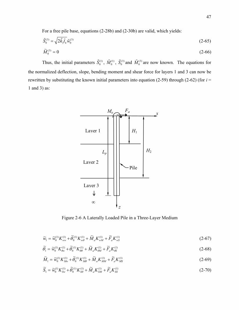
47
For a free pile base, equations (2-28b) and (2-30b) are valid, which yields:
(3) (3)0 3 4 02S k t w= (2-65)
0~ )3(0 =M (2-66)
Thus, the initial parameters (1)0S , (1)
0M , (3)0S and (3)
0M are now known. The equations for
the normalized deflection, slope, bending moment and shear force for layers 1 and 3 can now be
rewritten by substituting the known initial parameters into equation (2-59) through (2-62) (for i =
1 and 3) as:
z
Ma
Lp
H1
H2
Layer 1
Fa
Pile
x
∞
Layer 2
Layer 3
Figure 2-6 A Laterally Loaded Pile in a Three-Layer Medium
)1()1()1()1(0
)1()1(01
~~~~~wSawMawww KFKMKKww +++= θθ (2-67)
)1()1()1()1(0
)1()1(01
~~~~~SaMaw KFKMKKw θθθθθ θθ +++= (2-68)
)1()1()1()1(0
)1()1(01
~~~~~MSaMMaMMw KFKMKKwM +++= θθ (2-69)
)1()1()1()1(0
)1()1(01
~~~~~SSaSMaSSw KFKMKKwS +++= θθ (2-70)

48
(3) (3) (3) (3) (3) (3) (3) (3) (3) (3)3 0 0 3 4 0 0 02ww w wS ww ww w K K k t w K w K Kθ θθ θ′= + + = + (2-71)
(3) (3) (3) (3) (3) (3) (3) (3) (3) (3)3 0 0 3 4 0 0 02w S ww K K k t w K w K Kθ θθ θ θ θθθ θ θ′= + + = + (2-72)
(3) (3) (3) (3) (3) (3) (3) (3) (3) (3)3 0 0 3 4 0 0 02Mw M MS Mw MM w K K k t w K w K Kθ θθ θ′= + + = + (2-73)
(3) (3) (3) (3) (3) (3) (3) (3) (3) (3)3 0 0 3 4 0 0 02Sw S SS Sw SS w K K k t w K w K Kθ θθ θ′= + + = + (2-74)
where (3) (3) (3)* * 3 4 *2w w SK K t k K′ = + . Equations (2-67) through (2-70) are valid for layer 1 while
equations (2-71) through (2-74) are valid for layer 3.
Now we impose the interface boundary conditions on the initial parameters. This leads to
a set of algebraic equations consisting of the unknown influence coefficients and initial
parameters. In our example problem, there are two interfaces (z = H1 and z = H2), and the
boundary conditions at these interfaces are given by equations (2-23b) through (2-26b) with i = 1
and 2 for z = H1 and z = H2, respectively. There are four equations per interface, resulting in
eight simultaneous equations, which can be written in matrix form as: (1) (1)
(1) (1)
(1) (1)
(1) (1)
(2) (2) (2) (2)
(2) (2) (2) (2)
(2) (2) (2) (2) (3) (3)
(2) (2) (2) (2
1 0 0 0 0 00 1 0 0 0 00 0 1 0 0 00 0 0 1 0 0
0 0 1 00 0 0 10 00 0
ww w
w
Mw M
Sw S
ww w wM wS
w M S
Mw M MM MS Mw M
Sw S SM SS
K KK KK KK K
K K K KK K K KK K K K K KK K K K
θ
θ θθ
θ
θ
θ
θ θθ θ θ
θ θ
θ
−−
−−
−−
′− −
(1)0(1)0(2)0(2)
0(2)0(2)0(3)0
) (3) (3) (3)0
Sw S
w
w
MSw
K K θ
θ
θ
θ
⎡ ⎤ ⎡ ⎤⎢ ⎥ ⎢ ⎥⎢ ⎥ ⎢ ⎥⎢ ⎥ ⎢ ⎥⎢ ⎥ ⎢ ⎥⎢ ⎥ ⎢ ⎥⎢ ⎥ ⎢ ⎥⎢ ⎥ ⎢ ⎥⎢ ⎥ ⎢ ⎥⎢ ⎥ ⎢ ⎥⎢ ⎥ ⎢ ⎥
′⎢ ⎥ ⎢ ⎥− −⎣ ⎦ ⎣ ⎦(1) (1)
(1) (1)
(1) (1)
(1) (1)
0000
a wM a wS
a M a S
a MM a MS
a SM a SS
M K F KM K F KM K F KM K F K
θ θ
⎡ ⎤− −⎢ ⎥− −⎢ ⎥⎢ ⎥− −⎢ ⎥− −⎢ ⎥= ⎢ ⎥
⎢ ⎥⎢ ⎥⎢ ⎥⎢ ⎥⎢ ⎥⎣ ⎦
(2-75)
We refer to equation (2-75) as the “matrix equation”. In the matrix equation, the first
four rows are valid at z = H1 while the remaining four are valid at z = H2. If, in equation (2-75),
we assume that the influence coefficients (K’s) are known, then all the unknown initial
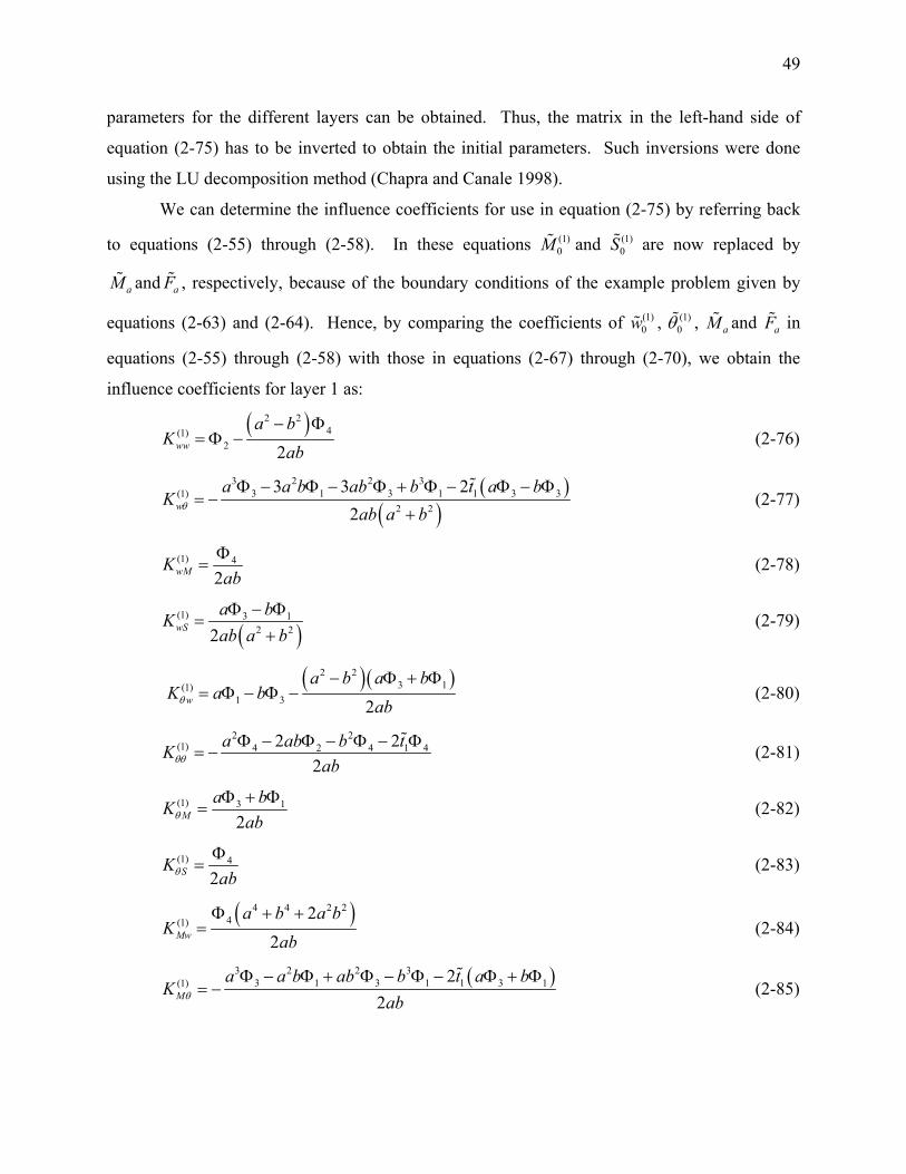
49
parameters for the different layers can be obtained. Thus, the matrix in the left-hand side of
equation (2-75) has to be inverted to obtain the initial parameters. Such inversions were done
using the LU decomposition method (Chapra and Canale 1998).
We can determine the influence coefficients for use in equation (2-75) by referring back
to equations (2-55) through (2-58). In these equations (1)0M and (1)
0S are now replaced by
aM and aF , respectively, because of the boundary conditions of the example problem given by
equations (2-63) and (2-64). Hence, by comparing the coefficients of (1)0w , (1)
0θ , aM and aF in
equations (2-55) through (2-58) with those in equations (2-67) through (2-70), we obtain the
influence coefficients for layer 1 as:
( )2 24(1)
2 2ww
a bK
ab− Φ
= Φ − (2-76)
( )( )
3 2 2 33 1 3 1 1 3 3(1)
2 2
3 3 22w
a a b ab b t a bK
ab a bθ
Φ − Φ − Φ + Φ − Φ − Φ= −
+ (2-77)
(1) 4
2wMKabΦ
= (2-78)
( )(1) 3 1
2 22wSa bKab a bΦ − Φ
=+
(2-79)
( )( )2 2
3 1(1)1 3 2w
a b a bK a b
abθ
− Φ + Φ= Φ − Φ − (2-80)
2 2(1) 4 2 4 1 42 2
2a ab b tK
abθθΦ − Φ − Φ − Φ
= − (2-81)
(1) 3 1
2Ma bK
abθΦ + Φ
= (2-82)
(1) 4
2SKabθΦ
= (2-83)
( )4 4 2 24(1)
22Mw
a b a bK
abΦ + +
= (2-84)
( )3 2 2 33 1 3 1 1 3 1(1) 2
2M
a a b ab b t a bK
abθ
Φ − Φ + Φ − Φ − Φ + Φ= − (2-85)

50
( )2 24 2(1)
22MM
a b abK
ab− Φ + Φ
= (2-86)
(1) 3 1
2MSa bK
abΦ + Φ
= (2-87)
{( )}
(1) 5 4 3 2 2 3 4 53 1 3 1 3 1
3 2 2 31 3 1 3 1
1 2 22
2
SwK a a b a b a b ab babt a a b ab b
= − Φ + Φ + Φ + Φ + Φ + Φ
− Φ − Φ + Φ − Φ (2-88)
( )4 2 2 4 2 21(1) 2
1 4
2 42
2S
a a b b t a bK t
abθ
⎧ ⎫+ + − −⎪ ⎪= − − Φ⎨ ⎬⎪ ⎪⎩ ⎭
(2-89)
( )3 2 2 33 1 3 1 1 3 1(1) 3 3 2
2SM
a a b ab b t a bK
abΦ + Φ − Φ − Φ − Φ + Φ
= (2-90)
2 2(1) 4 2 4 1 42 2
2SSa ab b tK
abΦ + Φ − Φ − Φ
= (2-91)
For the second (middle) layer, the following equations need to be solved simultaneously
in terms of C1, C2, C3 and C4 (note that these constants are different from the constants of layer
1):
44332211)2(
0~ φφφφ CCCCw +++= (2-92)
( ) ( ) ( ) ( )134243312421)2(
0~ φφφφφφφφθ baCbaCbaCbaC ++++−+−= (2-93)
( ){ } ( ){ }4222
23122
1)2(
0 2 2 ~ φφφφ abbaCabbaCM −−+−−=
( ){ } ( ){ }2422
41322
3 2 2 φφφφ abbaCabbaC +−++−+ (2-94)
( ) ( ){ } ( ) ( ){ }322
122
2422
222
1)2(
0 3 3 3 3 ~ φφφφ abbbaaCabbbaaCS −+−+−+−=
( ) ( ){ } ( ) ( ){ }1223
2242
224
223 3 3 3 3 φφφφ abbbaaCabbbaaC −−−+−−−+
( ) ( ) ( ) ( ){ }2 1 2 4 2 1 3 3 4 2 4 3 1 2 t C a b C a b C a b C a bφ φ φ φ φ φ φ φ− − + − + + + + (2-95)
where φ1, φ2, φ3 and φ4 are the values of Φ1, Φ2, Φ3 and Φ4, respectively, at the initial section of
the second layer (i.e., at z = H1). After obtaining the expressions of C1, C2, C3 and C4, the same
procedure as for layer 1 needs to be followed to obtain the influence coefficients of layer 2.
Similarly, the influence coefficients of layer 3 can be obtained by solving the following
equations for C1, C2, C3 and C4:
44332211)3(
0~ φφφφ CCCCw +++= (2-96)

51
( ) ( ) ( ) ( )134243312421)3(
0~ φφφφφφφφθ baCbaCbaCbaC ++++−+−= (2-97)
( ){ } ( ){ }(3) 2 2 2 20 1 1 3 2 2 40 2 2 M C a b ab C a b abφ φ φ φ= = − − + − −
( ){ } ( ){ }2 2 2 23 3 1 4 4 2 2 2C a b ab C a b abφ φ φ φ+ − + + − + (2-98)
( ) ( ){ }(3) (3) 2 2 2 20 3 4 0 1 2 42 3 3S k t w C a a b b b aφ φ= = − + −
( ) ( ){ } ( ) ( ){ }2 2 2 2 2 2 2 22 1 3 3 4 23 3 3 3 C a a b b b a C a a b b b aφ φ φ φ+ − + − + − − −
( ) ( ){ } ( ) ( ){2 2 2 24 3 1 3 1 2 4 2 1 33 3 2C a a b b b a t C a b C a bφ φ φ φ φ φ+ − − − − − + −
( ) ( )}3 4 2 4 3 1C a b C a bφ φ φ φ+ + + + (2-99)
where φ1, φ2, φ3 and φ4 are the values of Φ1, Φ2, Φ3 and Φ4, respectively at z =1.
Once the influence coefficients are known, the unknown initial parameters are
determined by solving equation (2-75). The initial parameters and influence coefficients are then
used to find the normalized pile deflection, slope, bending moment and shear force at any pile
section by using equations (2-67) through (2-70) for layer 1, (2-59) through (2-62) for layer 2
(with i = 2), and (2-71) through (2-74) for layer 3.
Evidently, MIP can be used for solving problems with any number of layers and for
different boundary conditions. It is important to note that the matrix equations for the different
cases (arising due to soil layering and pile boundary conditions) are different. However, for a
given pile head boundary condition, the influence coefficients for the top layer are the same
irrespective of the number of soil layers and of the boundary conditions at the pile base.
Similarly, for the bottom layer, the influence coefficients are independent of the number of soil
layers and of the pile head boundary conditions. Likewise, for any intermediate layer, the
expressions of the influence coefficients are the same irrespective of the pile head and base
boundary conditions and the number of layers present. This makes the determination of the
influence coefficient expressions and subsequent programming easy because the expressions for
the top and bottom layers do not vary from problem to problem if the boundary conditions
remain the same, and the expressions for intermediate layers are always the same, being also
independent of the head and base boundary conditions.

52
The influence coefficients and matrix equations for one-, two-, three- and four-layer soil
deposits have been obtained for all possible boundary conditions (i.e., free or fixed pile head
with free or fixed pile base). The expressions are given in Basu (2006).
2.7. Solution for Long Piles
2.7.1. General Solution
Long piles are piles whose response is identical to that of infinitely long piles. For such
piles, the boundary conditions at the pile base do not affect the pile response. Pile response
depends on the relative magnitudes of the pile and soil stiffness and on the pile geometry (pile
slenderness ratio). Depending on such ratios, as illustrated in Figure 2-7, a pile of length 5 m
may behave as a long pile, while a 10-m-long pile may not.
Figure 2-7a shows the deflection versus depth profiles of a set of 500-mm-diameter
concrete piles (Ep = 2.4 × 10⁶ kPa) of lengths 2.5 m, 5 m and 6 m, respectively, embedded in a
dense sand layer (k = 130 MPa, and t = 7.9 MN). A horizontal load of 100 kN is applied to all
the piles at the pile head. The piles are assumed to be free at the head; however, both free and
fixed conditions for the base are considered. It is evident from Figure 2-7a that the deflection
profile of the 5 m-long pile is independent of the pile base conditions and that the pile behaves as
a long pile. This happens because the ground is stiff enough when compared to the pile so that it
prevents lateral movement of the pile beyond a certain depth hf (= 3.3 m in this example), known
as the depth of fixity, which is less than the length of the pile. The 6-m-long pile also behaves as
a long pile because the depth of fixity remains at 3.3 m, which is less than the pile length (Figure
2-7a). However, the response of the 2.5-m-long pile depends on the base condition because the
pile has a length less than the depth of fixity; consequently, it does not behave as a long pile.
Figure 2-7b shows the deflection versus depth profile of a 1-m-diameter concrete pile of
length 10 m, embedded in a soft clay deposit with k = 11.6 MPa and t = 6.8 MN and subjected to
a 100 kN horizontal load at the head. The pile head is assumed to be free, while both free and
fixed conditions are considered for the base. The deflection profile clearly shows the influence
of the pile base condition, which is a contrast to the response of the 5-m-long pile of Figure 2-6a
(note that both the 5-m and 10-m piles have the same slenderness ratio). This indicates that the

53
10-m-long pile in clay does not behave as a long pile and that the depth of fixity hf is greater than
the length of the pile. Thus, the greater the ratio of pile to soil stiffness is, the larger the depth of
fixity is and the larger the length required for a pile to behave as a long pile is.
For long piles, the solution given by equation (2-40) must be modified. This is required
because, for long piles, the exponential terms with positive exponents (i.e., the terms containing aze or bze ) in the functions Φ1, Φ2, Φ3 and Φ4 (Table 2-1) become excessively large for
sufficiently large z (note that, the stiffer the soil, the greater the values of k, t, a and b are) and
the solution no longer represents the actual physical problem. The reason why this happens is
that, for long piles, the exponential terms with negative exponents (i.e., the terms containing aze− or bze− ) become negligible beyond a threshold value of z and cannot balance the effects of
the extremely large positive exponential terms. This makes the general solution unacceptable
because the pile deflection, and thus the functions Φ1, Φ2, Φ3 and Φ4, should decrease with
increasing z, while the positive exponential terms produce the opposite result.
The solution of equation (2-16b) or of equation (2-17b) for k i > ti2, when rewritten by
uncoupling the positive and negative exponential terms of the hyperbolic functions (Table 2-1),
leads to: ( ) ( ) ( ) ( )1 2 3 4( ) cos sin cos sinaz i i az i i
iw z e C bz C bz e C bz C bz− ⎡ ⎤ ⎡ ⎤= + + +⎣ ⎦ ⎣ ⎦ (2-100)
But, as z → 1 (z → Lp), 0~ →iw (i.e., as the depth z gets closer to the pile base, the
deflection decreases and approaches a zero value). This condition can be satisfied only if the
constants C3(i) and C4
(i) are each identically equal to zero because, otherwise, the term aze will
dominate (i.e., it will increase greatly with increases in z and produce large values of iw~ ).
Consequently, we get only two functions Φ1 and Φ2, associated with the negative exponent term,
as the solutions for equation (2-16b) and for equation (2-17b) with ki > t i2. The solution for
equation (2-17b) with ki < t i2 can be similarly written by decoupling the positive and negative
exponents as: ( ) ( ) ( ) ( )1 2 3 4( ) i az i bz i az i bz
iw z C e C e C e C e− −= + + + (2-101)
Following similar logic as for equation (2-100), the constants C3(i) and C4
(i) in equation
(2-101) are zero, and again we get only two functions which contain the negative exponential
terms. Thus, for long piles, the general solution can be written as:

54
2)(
21)(
1)~(~ Φ+Φ= iii CCzw (2-102)
The details of the functions Φ1 and Φ2 and their derivatives are given in Table 2-2.
The reduction of the solution functions from four to two can be explained using linear
algebra as well. The arguments az or bz of the hyperbolic functions in Table 2-1 have values
greater than 3 for values of z corresponding to depths greater than the depth of fixity. For such
values of arguments, hyperbolic sine and cosine functions give almost identical results (i.e., the
functions, when plotted, fall on top of each other for arguments greater than 3). Since functions
can be treated as vectors in linear algebra, the solution 4)(
43)(
32)(
21)(
1)~(~ Φ+Φ+Φ+Φ= iiiii CCCCzw
can be assumed to represent a vector space (Strang 1988) with the linearly-independent vectors
Φ1, Φ2, Φ3 and Φ4 (the functions Φ1, Φ2, Φ3 and Φ4 are linearly independent because they are
solutions of linear differential equations) forming the basis of the four-dimensional vector space.
However, when two of the functions become equal to the other two (i.e., sinhaz = coshaz and
sinhbz = coshbz ), there are only two linearly-independent vectors, and the four-dimensional
solution (vector) space collapses to a two-dimensional space. Consequently, we need only two
functions to produce the required solution.

55
hf
-0.4 0 0.4 0.8 1.2 1.6 2
Pile Deflection (mm)
6
4
2
0
Dep
th, z
(m)
5-m- and 6-m-long pile, both fixed and free base
2.5-m-long pile, free base
2.5-m-long pile, fixed base
(a)
-2 0 2 4 6-1 1 3 5
Pile Deflection (mm)
10
8
6
4
2
0
Dep
th, z
(m)
Free BaseFixed Base
(b)
Figure 2-7 Piles in (a) Dense Sand and (b) Soft Clay

56
Table 2-2 Functions in Equation (2-102) for Infinitely Long Piles Crossing Multiple Soil Layers
Con
stan
ts a
and
b
Individual Solutions of Equation
(2-17b)
Rel
ativ
e M
agni
tude
s of k a
nd t
a
b Func
tions
and
The
ir D
eriv
ativ
es
(prim
e (′)
indi
cate
s diff
eren
tiatio
n)
Φ1 Φ2
Φ zbe za ~cos~− zbe za ~sin
~−
Φ′ 21 Φ−Φ− ba 12 Φ+Φ− ba
Φ″ ( ) 1
22 Φ− ba
22 Φ+ ab
( ) 222 Φ− ba
12 Φ− ab
k >
t 2
√{½
(√k
+ t)
}
√{½
(√k −
t)}
Φ′″ ( ) 1
22 3 Φ−− baa+
( ) 222 3 Φ− abb
( ) 222 3 Φ−− baa
−
( ) 122 3 Φ− abb
Φ zae~− zbe
~−
Φ′ 1Φ− a 2Φ−b
Φ″ 12Φa 2
2Φb
Con
tinuu
m o
r Tw
o-Pa
ram
eter
Mod
el
k <
t 2
√{t +
√ (t 2 −
k)}
√{t −
√ (t 2
− k)}
Φ′″ 13Φ− a 2
3Φ−b
Note: For the individual solutions of equation (2-16b) (i.e., for the one-parameter model), the
functions Φ1 and Φ2 are the same as for the case k > t 2 in Table 2-2, but 4 4a b k= = .

57
2.7.2. Method of Initial Parameters
Application of MIP to equation (2-102) requires modifications to the method described
earlier, although the procedure, in principle, is the same. The solution procedure using MIP is
simple in case of a homogeneous soil deposit; however, for layered deposits, MIP equations will
be different depending on the location of the depth of fixity. For layers deeper than the depth of
fixity hf (and, indeed, for portions of a layer deeper than it), the MIP equations are not the same
as the equations derived earlier, which apply to z < hf .
In order to perform the analysis, it is essential to know whether a pile falls under the
category of long (infinite) pile or not (i.e., whether or not the depth of fixity is less than the pile
length). Such studies for beams on elastic foundations (i.e., whether a beam on elastic
foundation behaves as an infinite beam so that its boundary conditions do not affect its response)
have been studied by several authors. For example, Hetényi (1946) suggested that, for a beam
on a one-parameter foundation, if the length lb of the beam is greater than π/λb, where
4 4b b bk E Iλ = (k is the soil spring constant per unit beam length, Eb is the beam Young’s
modulus and Ib is the second moment of inertia of beam section), then the beam behaves as an
infinite beam. Vesić (1961), on the other hand, suggested that lb should be greater than 5/λb for a
beam on a one-parameter foundation to behave as an infinite beam. Similar limits are available
for beams on two-parameter foundations as well (Vlasov and Leont’ev 1966). However, these
limits were obtained by considering some specific examples (with specific loading conditions
and specific values of foundation parameters) and comparing the responses of beams of different
lengths for those specific conditions. Consequently, the limits suggested by these authors are
applicable to some specific cases; the limits change with loading condition and foundation
parameters. Moreover, these limits were obtained for infinite beams for which both the beam
ends are at infinite distance from the applied loads, while a long laterally loaded pile behaves as
a semi-infinite beam with only one end far away from the applied loads. Fleming et al. (1992)
suggested that the depth of fixity of laterally loaded piles in a one-parameter foundation is 4/λp
where 4 4p p pk E Iλ = . Poulos and Davis (1980) suggested that the depth of fixity is 2.5/λp and
1.5/λp for free-head and fixed-head piles, respectively. Clearly, there is no consensus in the
literature regarding the issue, and no limit for the depth of fixity for piles in two-parameter
foundation is available. Additionally, these limits for beams and piles were proposed based on

58
the assumption of a homogeneous deposit (i.e., with one value for k and one value for t
throughout), while, in our case, we have a layered deposit. For these reasons, these limits,
proposed for beams and piles, cannot be adapted in our study. The criterion adapted in this
thesis to identify depths greater than the depth of fixity (i.e., to identify long piles) is the
following: if, at any depth z within a layer i, 3ia z > or 3ib z > (a value slightly higher but not
greater than 3.5 can be used as well), then the depth of fixity corresponds to that depth z. Thus,
piles longer than that depth behave as long piles. This criterion is mathematically rigorous, as
explained before, and is easily applicable for layered media.
The MIP equations for equation (2-102) can be developed by following a similar
procedure as was followed before for equation (2-40). Since there are only two constants now,
only two initial parameters are required. For any layer i, the new MIP equations are given by:
( ) ( ) ( ) ( ) ( )0 0i i i i
i ww ww z w K K θθ= + (2-103)
( ) ( ) ( ) ( ) ( )0 0i i i i
i wz w K Kθ θθθ θ= + (2-104)
( ) ( ) ( ) ( ) ( )0 0i i i i
i Mw MM z w K K θθ= + (2-105)
( ) ( ) ( ) ( ) ( )0 0i i i i
i Sw SS z w K K θθ= + (2-106)
In order to illustrate how MIP works for long piles, we will again consider the same
example of a three-layer soil (Figure 2-5) with ki > ti2 for all the layers. The pile head is assumed
to be free; however, no condition for pile base is required to be stated explicitly because, for long
piles, the base is so far away from the influence of the applied force or moment that the
deflection, slope, bending moment and shear force at the base are all equal to zero. We will
further assume that the depth of fixity lies in the second (middle) layer. In other words, the
arguments az and bz become greater than 3 in the second layer. Thus, the MIP equations
corresponding to the top layer, as described before in the example, are all valid, while, for the
second and the third (bottom) layers new equations need to be developed.
A point to be noted here is that, although az and bz are assumed to become greater than 3
in the middle layer in this example, they are not necessarily greater than 3 in the bottom layer
(this can happen if the bottom layer consists of soft or loose soil so that the values of a and b are
lower than 3). However, equation (2-102) is still valid for the bottom layer (even if az and bz are
less than 3) because, once the depth of fixity is reached for any layer, deflections can only

59
decrease with further increase in z (which means that the positive exponential terms should be
omitted).
As before, we first choose the initial sections for each soil layer. For the top layer, the
pile head is chosen as the initial section. For the bottom layer, the pile base cannot be chosen as
the initial section because the corresponding initial parameters (i.e., the deflection and slope at
pile base) are already known to be zero. So, for both the middle and the bottom layers, we
choose the upper interfaces as the initial sections. Thus, the initial sections in the example are at
z = 0 for the top layer, at z = H1 for the middle layer and at z = H2 for the bottom layer. The
initial parameters are (1)0w , (1)
0θ , (1)0M and (1)
0S for the top layer, (2)0w and (2)
0θ for the middle
layer, and (3)0w and (3)
0θ for the bottom layer.
Next, we impose the boundary conditions. Imposing boundary conditions at the pile head
results in equations (2-63) and (2-64). This leads to equations (2-67) through (2-70) again
describing the top layer. The pile base boundary conditions have already been used up in
obtaining equation (2-102). Using the interface boundary conditions at H1 and H2, we get the
following matrix equation: (1) (1) (1)
0(1) (1) (1)
0(1) (1) (2) (2) (2)
0(1) (1) (2) (2) (2)
0(2) (2) (3)
0(2) (2) (3)
0
1 0 0 00 1 0 0
0 00 0
0 0 1 00 0 0 1
ww w
w
Mw M Mw M
Sw S Sw S
ww w
w
K K wK KK K K K wK K K K
K K wK K
θ
θ θθ
θ θ
θ θ
θ
θ θθ
θ
θ
θ
⎡ ⎤ ⎡ ⎤−⎢ ⎥ ⎢ ⎥−⎢ ⎥ ⎢ ⎥⎢ ⎥ ⎢ ⎥− −⎢ ⎥ ⎢ ⎥
− −⎢ ⎥ ⎢ ⎥⎢ ⎥ ⎢ ⎥−⎢ ⎥ ⎢ ⎥
−⎢ ⎥ ⎢ ⎥⎣ ⎦ ⎣ ⎦
(1) (1)
(1) (1)
(1) (1)
(1) (1)
00
a wM a wS
a M a S
a MM a MS
a SM a SS
M K F KM K F KM K F KM K F K
θ θ
⎡ ⎤− −⎢ ⎥− −⎢ ⎥⎢ ⎥− −
= ⎢ ⎥− −⎢ ⎥
⎢ ⎥⎢ ⎥⎢ ⎥⎣ ⎦
(2-107)
In the above matrix equation, the first four rows are valid at z = H1 while the remaining two are
valid at z = H2.
The influence coefficients can be obtained as before. Equations (2-76) through (2-91)
give the influence coefficients for the top layer. In order to obtain the influence coefficients for
the middle (second) layer, we refer back to equation (2-102). The normalized pile deflection,
slope, bending moment and shear force can be obtained from equation (2-102) and its derivatives
(see Table 2-2 under k > t 2 for the differentiations of Φ1 and Φ2) as:
22112~ Φ+Φ= CCw (2-108)
( ) ( )1222112~
Φ+Φ−+Φ+Φ−= baCbaCθ (2-109)

60
( ){ } ( ){ }1222
22122
12 2 2 ~ Φ−Φ−+Φ+Φ−= abbaCabbaCM (2-110)
( ) ( ){ } ( ) ( ){ }1222
2222
221
2212 3 3 3 3 ~
Φ−−Φ−−+Φ−+Φ−−= abbbaaCabbbaaCS
( ) ( ){ }1222111 ~2 Φ+Φ−+Φ+Φ−− baCbaCt (2-111)
where the constants C1 and C2 are valid for the second layer.
We solve equations (2-108) and (2-109) for C1 and C2 at the initial section of the second
layer (i.e., at z = H1):
2211)2(
0~ φφ CCw += (2-112)
( ) ( )122211)2(
0~ φφφφθ baCbaC +−++−= (2-113)
where φ1 and φ2 are the values of Φ1 and Φ2 (Table 2-2) at z = H1. Solving equations (2-112) and
(2-113), we get:
( )( )
(2) (2)0 1 2 0 2
1 2 21 2
w b aC
bφ φ θ φφ φ− −
=+
(2-114)
( )( )
(2) (2)0 1 2 0 1
2 2 21 2
w a bC
bφ φ θ φφ φ+ +
=+
(2-115)
Substituting the constants C1 and C2 into equations (2-108) through (2-111) and
comparing the coefficients of (2)0w and (2)
0θ in these four equations with those in equations (2-
103) through (2-106) (with i = 2), we obtain the influence coefficients for the middle layer. The
influence coefficients for the bottom layer can be obtained following similar steps, and, in fact,
the expressions are identical to those of the middle layer (with the exception that φ1 and φ2 are
the values of Φ1 and Φ2 at z = H2).
Using the values of the influence coefficients, the unknown initial parameters are
determined by solving equation (2-107). The initial parameters and the influence coefficients are
then used to find the normalized pile deflection, slope, bending moment and shear force at any
pile section by using equations (2-67) through (2-70) for layer 1 and by using equations (2-103)
through (2-106) for layers 2 (with i = 2) and 3 (with i = 3), respectively.
The influence coefficients and matrix equations for up to four layers, with the depth of
fixity lying in the first, second, third or fourth layers have been obtained for free or fixed pile
head conditions and can be readily used.
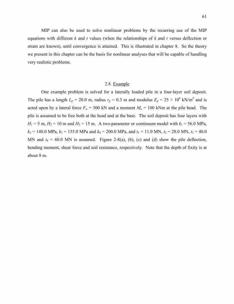
61
MIP can also be used to solve nonlinear problems by the recurring use of the MIP
equations with different k and t values (when the relationships of k and t versus deflection or
strain are known), until convergence is attained. This is illustrated in chapter 8. So the theory
we present in this chapter can be the basis for nonlinear analyses that will be capable of handling
very realistic problems.
2.8. Example
One example problem is solved for a laterally loaded pile in a four-layer soil deposit.
The pile has a length Lp = 20.0 m, radius rp = 0.3 m and modulus Ep = 25 × 106 kN/m2 and is
acted upon by a lateral force Fa = 300 kN and a moment Ma = 100 kNm at the pile head. The
pile is assumed to be free both at the head and at the base. The soil deposit has four layers with
H1 = 5 m, H2 = 10 m and H3 = 15 m. A two-parameter or continuum model with k1 = 56.0 MPa,
k2 = 140.0 MPa, k3 = 155.0 MPa and k4 = 200.0 MPa, and t1 = 11.0 MN, t2 = 28.0 MN, t3 = 40.0
MN and t4 = 60.0 MN is assumed. Figure 2-8(a), (b), (c) and (d) show the pile deflection,
bending moment, shear force and soil resistance, respectively. Note that the depth of fixity is at
about 8 m.

62
-1 0 1 2 3 4
Pile Deflection (mm)
20
16
12
8
4
0
Dep
th, z
(m)
-50 0 50 100 150 200 250
Bending Moment (kNm)
20
16
12
8
4
0
Dep
th, z
(m)
-100 0 100 200 300
Shear Force (kN)
20
16
12
8
4
0
Dep
th, z
(m)
-50 0 50 100 150 200
Soil Resistance (kN/m)
20
16
12
8
4
0D
epth
, z (m
)
Figure 2-8 (a) Deflection, (b) Bending Moment, (c) Shear Force and (d) Soil Resistance of a Laterally Loaded Pile
2.9. Summary
The governing differential equations and boundary conditions for laterally loaded piles
embedded in layered elastic media were developed following a beam-on-elastic-foundation
(c) (d)
(b) (a)

63
approach. The method of initial parameters, traditionally used to solve problems of beams on
elastic foundations, was then modified to obtain analytically the pile deflection, slope, bending
moment and shear force as functions of depth. The method was illustrated using an example of a
laterally loaded pile embedded in a three-layer soil deposit.

64
CHAPTER 3. CONTINUUM ANALYSIS OF LATERALLY LOADED PILE IN LAYERED ELASTIC MEDIUM
3.1. Introduction
In this chapter, we develop a method of analysis for a laterally loaded pile embedded in a
multi-layered soil deposit by treating the soil deposit as a three-dimensional, elastic continuum.
We apply the principle of minimum potential energy to obtain the governing differential
equations for deflection of pile and displacements in the continuum, after making some
simplified assumption regarding the displacement field within the elastic medium. The resulting
differential equations describing the pile deflection and soil displacements are interdependent,
showing that the analysis takes explicit account of the soil-structure interaction.
The differential equations governing the pile deflection function and the boundary
conditions are exactly the same as the corresponding equations obtained for the two-parameter
foundation model in chapter 2. Thus, we show a one-to-one correspondence between the
continuum-based approach and the beam-on-elastic-foundation approach for laterally loaded
piles in layered media. Moreover, the analysis developed in this chapter provides a rational basis
for the calculation of the parameters k and t for the elastic foundation models described in
chapter 2. Because of the correspondence between the two approaches, analytical solutions of
the pile deflection equations developed in this chapter can be obtained using the MIP, which was
described in chapter 2.
3.2. Overview
The beam-on-elastic foundation approach, outlined in chapter 2, can be efficiently used
for the analysis of laterally loaded piles in elastic soil if we can readily obtain the values of the
parameters k and t for different soils. The spring constant k can be determined from plate load
tests; but the limitation is that the obtained values of k are not unique because the values depend
on many factors like the size, shape and flexibility of the plate, depth at which the test is
65
performed and the rate of loading (Selvadurai 1979). Moreover, a plate load test determines the
vertical stiffness of ground, whereas, for laterally loaded piles, horizontal stiffness is required. A
few laterally loaded plate tests were performed by Georgiadis and Butterfield (1982) to obtain
both the parameters k and t (and their nonlinear variation with pile deflection) by fitting a two-
parameter foundation-model equation, proposed by Kerr (1964), to the experimental results.
However, performing such tests for routine projects is uneconomical and is not used in practice.
Efforts have been made to relate results of the standard penetration test (SPT) and the cone
penetration test (CPT) with the modulus of subgrade reaction (Anderson and Townsend 2001).
The pressuremeter test and the dilatometer test can also be used to estimate k; in fact, they have
been used to develop p-y curves (Gabr et al. 1994, Briaud 1997). But such correlations are
empirical and not generally applicable. Thus, there is no easy and rational way of directly
determining the value of k or t that is applicable for laterally loaded pile analysis. In fact, most
researchers neglect the shear parameter (i.e., assume a one-parameter model). Some authors,
based on experience and back calculation of numerical analyses, have proposed some bulk-part
values (or range of values) of k for different soils (Poulos and Davis 1980, Scott 1981, Bowles
1997). Similar empirical approach is adopted to develop the p-y curves as well (Reese and Cox
1969, Matlock 1970, Reese et al. 1974, 1975).
Clearly, improvements in estimating the soil parameters are necessary if realistic
predictions for lateral deflections of piles are to be made. Such an effort for beams on elastic
foundations led several authors to develop empirical and semi-empirical relationships between
the parameter k and the elastic constants of the soil, namely, Young’s modulus Es and Poisson’s
ration υs (Vesić 1961, Biot 1937). The advantage of this approach is that the elastic constants
can be determined with reasonable accuracy from a variety of laboratory and field tests or
through simple correlations with easily measurable soil properties (Salgado 2008, Bowles 1997,
Selvadurai 1979), and typical values (or range of values) of the constants for different types of
soil are available in the literature (Selvadurai 1979, Rao 1998, Bowles 1997). However, the
available relationships relating k with Es and υs for beams are semi-empirical, and although
modifications of these expressions for laterally piles are available (Francis 1964, Hsiung and
Chen 1997, Ashford and Juirnarongrit 2003), these relationships are restrictive in their
applicability and not rigorous enough to be used reliably in design.

66
A rational method of analysis of beams on elastic foundations was developed by Vlasov
and Leont’ev (1966) based on an elastic continuum approach. Their analysis rigorously related
the two parameters k and t with the soil elastic constants Es and υs using variational principles.
These relationships are valid for any generalized loading and for all boundary conditions. In
their analysis, Vlasov and Leont’ev (1966) considered only vertical displacement within the
continuum (displacements in the horizontal directions were assumed to be zero) and expressed
the displacement as a product of two separable functions; an unknown function describing the
beam deflection and a known function describing the variation of displacement within the
continuum. Applying the principle of virtual work, Vlasov and Leont’ev (1966) obtained the
governing differential equation for the beam deflection function, which is exactly the same as the
equation for the two-parameter foundation. Improvement to this analysis was done by Rao et al.
(1971), who considered non-zero horizontal displacement in the foundation.
Vlasov and Leont’ev (1966) had assumed a known function that described the variation
of displacement with depth within the continuum. Vallabhan and Das (1988), (1991), following
a methodology adapted by Jones and Xenophontos (1977) for analyzing plates on elastic
foundations, improved the analysis of Vlasov and Leont’ev (1966) by letting the spatial function
be unknown to begin with, and then rigorously determined the function using variational
principles. This analysis framework was adapted by Sun (1993), (1994a), who applied it to
laterally loaded piles embedded in homogeneous elastic media. Guo and Lee (2001) modified
the analysis by assuming a simplified stress field in the continuum surrounding the pile;
however, such simplification led to empirical equations relating k and t with Es and υs. Yang et
al. (2002) extended the analysis of Sun (1994a) for a two-layer system; however, the boundary-
condition equations pertaining to shear force were incorrect, making the analysis unusable.
In the analysis of Sun (1994a), the assumption regarding the displacement field, that the
variation of displacements within the soil mass depends on the same displacement function for
both the radial and circumferential directions, leads to a soil response that is stiffer than it is in
reality. In this chapter, we adapt the basic methodology of Sun (1994a) but propose a new
displacement field by assuming different displacement functions for the radial and
circumferential directions that removes the artificial stiffness in the model of Sun (1994a). At
the same time, we extend the analysis to account for multi-layered soil. A similar attempt to

67
remove the artificial stiffness was made by Vallabhan (1999); however, the expressions obtained
in that paper are valid only for a single layer.
This analysis allows us to rationally link ki and ti with the Young’s modulus Esi and
Poisson’s ratio υsi for any layer i. It also shows how the resistive properties of soil elements (i.e.,
the stress-strain relationships) add together to produce the overall soil resistance against laterally
loaded pile movement. At the same time, the analysis forms the basis for future formulations
that can take into account the nonlinear stress-strain behavior of soil.
3.3. Analysis
3.3.1. Problem Definition
We consider a pile with a circular cross section of radius rp and length Lp embedded in a
soil deposit that has n layers (Figure 3-1). Each layer extends to infinity in all radial directions,
and the bottom (nth) layer extends to infinity in the downward direction. The vertical depth to
the base of any intermediate layer i is Hi, which implies that the thickness of the ith layer is Hi −
Hi−1 with H0 = 0. The pile head is at the ground surface, and the base is embedded in the nth
layer. The pile is subjected to a horizontal force Fa and a moment Ma at the pile head such that
Fa and Ma are orthogonal vectors.
In the analysis, we choose a cylindrical (r-θ-z) coordinate system with its origin
coinciding with the center of the pile head and the positive z-axis (coinciding with the pile axis)
pointing downward. The goal of the analysis is to obtain pile deflection as a function of depth
caused by the action of Fa and/or Ma at the pile head.
The soil medium is assumed to be isotropic, homogeneous within each layer, and linearly
elastic with Lame’s constants λs and Gs. There is no slippage or separation between the pile and
the surrounding soil or between the soil layers. The pile behaves as an Euler-Bernoulli beam
with a constant flexural rigidity EpIp.

68
2rp
r
r0
Fa
MaPile
θ
∞ H1
Hn-2
Hi Hi-1
H2
r0Ma
…
…
…
…
Hn-1
Layer 1
Layer 2
Layer i
Layer n−1
Layer n
z
Fa
Pile
Lp
∞
∞
Figure 3-1 A Laterally Loaded Pile in a Layered Elastic Medium
3.3.2. Potential Energy
The total potential energy of the pile-soil system, including both the internal and external
potential energies, is given by: 2 2 22
20 0 0 0 0
00
1 1 1 2 2 2
p p
p p
L r
p p pq pq pq pqr L
a azz
d wE I dz r dr d dz r dr d dzdz
dwF w Mdz
π π
σ ε θ σ ε θ∞ ∞ ∞
==
⎛ ⎞Π = + +⎜ ⎟
⎝ ⎠
− +
∫ ∫ ∫ ∫ ∫ ∫ ∫ (3-1)
where w is the lateral pile deflection; and σpq and εpq are the stress and strain tensors (see Figure
3-2) in the soil (summation is implied by the repetition of the indices p and q in the product of
corresponding stress and strain components). The first integral represents the internal potential
energy of the pile. The second and third integrals represent the internal potential energy of the
continuum (note that the third integral represents the energy of the column of soil with radius rp

69
starting at the pile base and extending to infinity downward, while the second integral represents
the energy of the soil surrounding both the pile and this column of soil). The remaining two
terms represent the external potential energy.
τzr
τθ r
τθ z
σrr
r0
θ τrz
τzθ
σzz
σθθ
z
τrθ
Figure 3-2 Stresses Within a Soil Continuum
3.3.3. Displacement Field
We assume the following displacement fields (Figure 3-3) in the soil:
( ) ( )cosr ru w z rφ θ= (3-2a)
( ) ( )sinu w z rθ θφ θ= − (3-2b)
0zu = (3-2c)
where w(z) is a displacement function (with a dimension of length), varying with depth z,
representing the deflection of the pile axis; φr(r) and φθ(r) are dimensionless displacement
functions varying with the radial coordinate r, and θ is the angle measured clockwise from a
vertical reference section (r = r0) that contains the applied force vector Fa. Note that the

70
reference plane r0-z coincides with the x-z plane of the x-y-z coordinate system (Figure 2-2)
assumed in chapter 2. Equation (3-2c) is based on the assumption that the vertical displacement
of the pile caused by the lateral load and moment applied at the pile head is negligible.
The functions φr(r) and φθ(r) describe how the displacements within the soil mass (due to
pile deflection) decrease with increasing radial distance from the pile axis. We set φr(r) = 1 and
φθ(r) = 1 at r = rp (this ensures compatibility at the pile-soil interface) and φr(r) = 0 and φθ(r) = 0
at r = ∞ (this ensures that displacements in the soil decrease with increasing radial distance from
the pile). Thus, φr and φθ vary between 1 at the pile-soil interface to 0 at infinite radial distance
from the pile.
θ
uθ
r0
z
ur uz
Fa
Figure 3-3 Displacements Within a Soil Continuum
3.3.4. Stress-Strain-Displacement Relationships
The strain-displacement relationship, considering equation (3-2), leads to:
( ) ( )
( ) ( ) ( )
( ) ( ) ( ) ( )
cos
1cos
0
sin1
1
r r
r rrr
z
zzr
r r
rz
z rz
z
u d rw zr dr
uu r rw zr r r
uz r r d r
w zu uur dr
r r rdu u
r zuu
r z
θ θ
θθ
θ θθ θ θ
θ
θ
φθ
φ φε θθεε
φ φ φθγ
θγγ
θ
∂⎡ ⎤− −⎢ ⎥∂⎢ ⎥∂ −⎢ ⎥− − −⎡ ⎤ ⎢ ⎥∂⎢ ⎥ ⎢ ⎥∂⎢ ⎥ ⎢ ⎥−⎢ ⎥ ⎢ ⎥∂= = −⎧ ⎫⎢ ⎥ ⎢ ⎥ +∂∂ ⎨ ⎬⎢ ⎥ ⎢ ⎥− − + ⎩ ⎭⎢ ⎥ ∂ ∂⎢ ⎥
⎢ ⎥ ⎢ ⎥∂ ∂⎢ ⎥ −⎣ ⎦ − −⎢ ⎥∂ ∂⎢ ⎥
⎢ ∂ ⎥∂− −⎢ ⎥∂ ∂⎣ ⎦
( ) ( )
( ) ( )
cos
sin
r
w zr
dzdw z
rdz θ
φ θ
φ θ
⎡ ⎤⎢ ⎥⎢ ⎥⎢ ⎥⎢ ⎥⎢ ⎥⎢ ⎥⎢ ⎥⎢ ⎥⎢ ⎥⎢ ⎥⎢ ⎥⎢ ⎥⎢ ⎥⎢ ⎥⎢ ⎥⎣ ⎦
(3-3)

71
The stress-strain relationship in any elastic layer is given by:
2 0 0 02 0 0 0
2 0 0 00 0 0 0 00 0 0 0 00 0 0 0 0
rr s s s s rr
s s s s
zz s s s s zz
r s r
rz s rz
z s z
GG
GG
GG
θθ θθ
θ θ
θ θ
σ λ λ λ εσ λ λ λ εσ λ λ λ ετ γτ γτ γ
+⎡ ⎤ ⎡ ⎤ ⎡ ⎤⎢ ⎥ ⎢ ⎥ ⎢ ⎥+⎢ ⎥ ⎢ ⎥ ⎢ ⎥⎢ ⎥ ⎢ ⎥ ⎢ ⎥+
=⎢ ⎥ ⎢ ⎥ ⎢ ⎥⎢ ⎥ ⎢ ⎥ ⎢ ⎥⎢ ⎥ ⎢ ⎥ ⎢ ⎥⎢ ⎥ ⎢ ⎥ ⎢ ⎥⎢ ⎥ ⎢ ⎥ ⎢ ⎥⎣ ⎦ ⎣ ⎦ ⎣ ⎦
(3-4)
Combination of equations (3-3) and (3-4) gives the strain energy density within any layer
as:
( ) ( )
( ) ( ) ( )
( )
22 2 2 2
2 22 2 2
2 2
22 2 2 2
1 1 2 cos 2 cos2 2
cos
sin 2 sin
rr rpq pq s s s
r rs s s
rs s
s
d dG w wdr dr r
G w G wr r
d dG w G wdr r dr
G
θ
θ θ
θθ θ
φ φφ φσ ε λ θ λ θ
φ φ φ φλ θ
φ φφ φθ θ
⎡ −⎛ ⎞= + +⎢ ⎜ ⎟⎝ ⎠⎢⎣
− −+ + +
−⎛ ⎞+ +⎜ ⎟⎝ ⎠
+2 2
2 2 2 2cos sinr sdw dwGdz dz θφ θ φ θ
⎤⎛ ⎞ ⎛ ⎞+ ⎥⎜ ⎟ ⎜ ⎟⎝ ⎠ ⎝ ⎠ ⎥⎦
(3-5)
Substituting equation (3-5) into equation (3-1), we get:
( )
( ) ( ) ( )
( )
2 222
20 0
2 22 2 2
2
2 22 2 2
1 2 2 2
2 3
2
+2
p
p
Lr
p p s sr
r rrs s s s
rs s r s
d w dE I dz G wdz dr
d dw G w G wdr r r dr
d dw dwG w G G rdrdzr dr dz dz
r
θ θ θ
θ θθ
π φλ
φ φ φ φφ φλ λ
φ φ φ φ φ
π
∞ ∞ ⎡⎛ ⎞ ⎛ ⎞Π = + +⎢⎜ ⎟ ⎜ ⎟⎝ ⎠⎢⎝ ⎠ ⎣
− − ⎛ ⎞+ + + + ⎜ ⎟⎝ ⎠
⎤− ⎛ ⎞ ⎛ ⎞+ + + ⎥⎜ ⎟ ⎜ ⎟⎝ ⎠ ⎝ ⎠ ⎥⎦
∫ ∫ ∫
22
00p
p s a azzL
dw dwG dz F w Mdz dz
∞
==
⎛ ⎞ − +⎜ ⎟⎝ ⎠∫
(3-6)
3.3.5. Principle of Minimum Potential Energy
A system in equilibrium exists with its potential energy at a minimum. Hence,
minimizing the potential energy of the pile-soil system (i.e., setting the first variation δΠ of the

72
potential energy equal to 0) produces the equilibrium equations. Applying δΠ = 0 to equation
(3-6), we get:
( )
( ) ( )
( )
22 2
2 20 0
22
2 2
2
2
2 2
2 3 3
2 3 2
p
p
Lr r r
p p s s sr
r rs s s s s
r rs s s s
d dd w d wE I dz G w w w wdz dz dr r dr
dw w G w w G w wr dr r r
d dG w w G w w G w wr dr r d
θ θ
θ θ θ
φ φ φδ π λ δ λ δ
φ φφ φλ δ λ δ λ δ
φ φ φ φφλ δ δ δ
∞ ∞⎧ ⎡⎛ ⎞⎪ ⎛ ⎞+ + +⎢⎨ ⎜ ⎟ ⎜ ⎟⎝ ⎠⎢⎝ ⎠⎪ ⎣⎩
− + + + +
⎛ ⎞− + + +⎜ ⎟⎝ ⎠
∫ ∫ ∫
( )
2 2
20
0
2 2
0
2
1 2
p
p
s s r s
p s a azL z
r rs s s r
r
rd dw dw dw dwG w w G G rdrdz
r dr dz dz dz dz
dw dw dwr G dz F w Mdz dz dz
d dG w wdr dr r
θ θθ
φ φδ δ φ δ φ
π δ δ δ
φ φπ λ δ λ δφ
∞
==
∞ ∞
⎤⎛ ⎞ ⎛ ⎞− + +⎜ ⎟ ⎜ ⎟ ⎥⎝ ⎠ ⎝ ⎠ ⎦⎫⎪⎛ ⎞ ⎛ ⎞+ − + ⎬⎜ ⎟ ⎜ ⎟
⎝ ⎠ ⎝ ⎠ ⎪⎭
⎡ ⎛ ⎞ ⎛ ⎞+ + +⎜ ⎟ ⎜ ⎟⎢ ⎝ ⎠ ⎝ ⎠⎣
∫
∫ ∫
( ) ( )
( )
2
2 2 22 2
22
2 22
0
3 3
1
1 3 3p
r r rs
r rs s s r s s r
s r s r r
rs s s s
r
d dwdr r dr
dw G w G wr dr r r
d dwG w G rdrdzr dr dz
dw G w Gr dr r
θ θ
θ
θθ θ
φ φ φλ δ
φ φφ φλ δ λ δφ λ δφ
φδφ φ δφ
φφπ λ δφ λ δφ λ∞ ∞
⎧⎪ ⎛ ⎞+⎨ ⎜ ⎟⎝ ⎠⎪⎩
⎛ ⎞− + + − +⎜ ⎟⎝ ⎠
⎫⎤ ⎪⎛ ⎞+ + ⎥ ⎬⎜ ⎟⎝ ⎠ ⎥ ⎪⎦ ⎭
⎧⎪+ − + + − +⎨⎪⎩∫ ∫ ( ) 2
2
2 2 2
22
1
0
rs
rs s s
s s
wr
d d d dG w G w G wdr dr r dr r dr
d dwG w G rdrdzr dr dz
θ
θ θ θ θθ
θ θθ θ
φ δφ
φ φ φ φφδ δ δφ
φ φδ φ δφ
⎛ ⎞ ⎛ ⎞+ + −⎜ ⎟ ⎜ ⎟⎝ ⎠ ⎝ ⎠
⎫⎤⎫⎪ ⎪⎛ ⎞ ⎛ ⎞− + =⎥⎬ ⎬⎜ ⎟⎜ ⎟⎝ ⎠⎝ ⎠ ⎥⎪ ⎪⎭⎦ ⎭
(3-7)
Simplifying further and considering a layered system (Figure 3-1):

73
1 2
1
1
4 2 4 21 1 2 2
1 1 1 1 2 2 2 24 2 4 20
4 2 21
1 1 14 2 2
31
2 2
.... 2 2
p
n p
H H
p p p pH
Ln n n
p p i i n n n n n nH L
p p
d w d w d w d wE I t k w w dz E I t k w w dzdz dz dz dz
d w d w d wE I t k w w dz t k w w dzdz dz dz
d wE I
δ δ
δ δ−
∞+
+ + +
⎧ ⎡ ⎤ ⎡ ⎤⎪ − + + − +⎨ ⎢ ⎥ ⎢ ⎥⎣ ⎦ ⎣ ⎦⎪⎩
⎡ ⎤ ⎡ ⎤+ + − + + − +⎢ ⎥ ⎢ ⎥
⎣ ⎦ ⎣ ⎦
+
∫ ∫
∫ ∫
1 1
1
21 1 1
1 13 200
3 31 1 2 2
1 1 2 23 3
2 21 1 2 2
2 2
2
2 2
a p p azz
p p p pz H z H
p p p pz H
dw d w dwt F w E I Mdz dz dz dz
d w dw d w dwE I t w E I t wdz dz dz dz
d w dw d w dwE I E Idz dz dz dz
δ δ
δ δ
δ δ
==
= =
=
⎡ ⎤ ⎡ ⎤ ⎛ ⎞− − − − ⎜ ⎟⎢ ⎥ ⎢ ⎥⎝ ⎠⎣ ⎦ ⎣ ⎦
⎡ ⎤⎛ ⎞ ⎛ ⎞+ − − + −⎢ ⎥⎜ ⎟ ⎜ ⎟
⎝ ⎠ ⎝ ⎠⎣ ⎦⎡ ⎛ ⎞ ⎛ ⎞+ −⎢ ⎜ ⎟ ⎜ ⎟
⎝ ⎠ ⎝ ⎠⎢⎣
( )
1
31
1 13
21
1 12
2
1 3 2 4 42
.... 2 2
2
p p
p
z H
n n np p n n n nz L z L
n n np p n n z
z L
r r rs s s s s s r
d w dw dwE I t w t wdz dz dz
d w dw dwE I t wdz dz dz
dd dm r m m m m n rdr dr dr r r
θ θ
δ δ
δ δ
φ φφ φ φ φ
=
++ += =
++ + =∞
=
⎤⎥⎥⎦
⎡ ⎤⎛ ⎞⎫+ + − − −⎬⎢ ⎥⎜ ⎟⎭⎝ ⎠⎣ ⎦
⎫⎪⎛ ⎞+ + ⎬⎜ ⎟⎝ ⎠ ⎪⎭
⎛ ⎞+ − + + + + − +⎜ ⎟
⎝ ⎠
( )
1 3 3
2
2 2 3 4 42
2 2 2
p
p pp
p
p pp
rr
rs r s r r s rr r
r
r rs s s s s s
r
s s r sr rr
dr
dm r m mdr
d d dm r m m m m n r drdr dr dr r r
dm r m mdr
θ
θ θ θθ θ
θθ θ θ θ
δφ
φ δφ φ δφ φ δφ
φ φ φφ φ φ δφ
φ δφ φ δφ φ δφ
∞
∞∞ ∞
∞
∞∞ ∞
⎧ ⎡ ⎤⎪⎨ ⎢ ⎥
⎣ ⎦⎪⎩⎫⎪+ + − ⎬⎪⎭
⎧ ⎡ ⎤⎛ ⎞⎪+ − + − + + − +⎨ ⎢ ⎥⎜ ⎟⎝ ⎠⎣ ⎦⎪⎩
⎫+ + − ⎬
∫
∫
0⎪ =⎪⎭
(3-8)
where
( )
( )
21 2
21 2
; 1, 2, ..., 2
1 ; 12
si p
i
sn p
G r i nt
G r i n
π ξ ξ
π ξ ξ
⎧ + =⎪⎪= ⎨⎪ + + = +⎪⎩
(3-9)
21 2
1
p
rp r
r drr
ξ φ∞
= ∫ (3-10)

74
22 2
1
pp r
r drr θξ φ
∞
= ∫ (3-11)
( ) ( ) ( )( )( )
1 2 3 5 4 6
7 8 9
2 2 2
3 2i si si si si si
si si
k G G G
G
π λ η η λ η η η η
λ η η η
= + + + − − −⎡⎣+ + + − ⎤⎦
(3-12)
2
1
p
r
r
dr drdrφη
∞ ⎛ ⎞= ⎜ ⎟⎝ ⎠∫ (3-13)
2
2
pr
dr drdr
θφη∞ ⎛ ⎞= ⎜ ⎟
⎝ ⎠∫ (3-14)
3
p
rr
r
d drdrφη φ
∞
= ∫ (3-15)
4
pr
d drdr
θθ
φη φ∞
= ∫ (3-16)
5
p
r
r
d drdrθφη φ
∞
= ∫ (3-17)
6
p
rr
d drdr
θφη φ∞
= ∫ (3-18)
27
1
p
rr
drr
η φ∞
= ∫ (3-19)
28
1
pr
drr θη φ
∞
= ∫ (3-20)
91
p
rr
drr θη φ φ
∞
= ∫ (3-21)
( ) ( )1
12 2
110
2 2i
i
Hn
s s s si si ii H
m G w dz G w dzλ λ−
∞ +
=
= + = +∑∫ ∫ (3-22)
1
12 2
210
i
i
Hn
s s si ii H
m G w dz G w dz−
∞ +
=
= =∑∫ ∫ (3-23)
1
12 2
310
i
i
Hn
s s si ii H
m w dz w dzλ λ−
∞ +
=
= =∑∫ ∫ (3-24)

75
( ) ( )1
12 2
410
3 3i
i
Hn
s s s si si ii H
m G w dz G w dzλ λ−
∞ +
=
= + = +∑∫ ∫ (3-25)
1
22 1
10
i
i
Hni
s s sii H
dwdwn G dz G dzdz dz
−
∞ +
=
⎛ ⎞⎛ ⎞= =⎜ ⎟ ⎜ ⎟⎝ ⎠ ⎝ ⎠
∑∫ ∫ (3-26)
The subscript i in the above equations refers to the ith layer of the multi-layered continuum
(Figure 3-1); wi represents the function w(z) in the ith layer with 1i i
i iz H z Hw w += =
= . Note that the
nth (bottom) layer is split into two parts with the part below the pile denoted by the subscript
n+1; therefore, in the above equations, Hn = Lp and Hn+1 → ∞.
Equation (3-8) is of the form:
( ) ( ) ( ){ } ( ){ } 0r rdwA w w B w C Ddz θ θδ δ δ φ δφ φ δφ⎧ ⎫⎛ ⎞Π = + + + =⎨ ⎬⎜ ⎟
⎝ ⎠⎩ ⎭ (3-27)
Since the variations δw(z), δ(dw/dz), δφr(r) and δφθ(r) of the functions w(z) (and its derivative),
φr(r) and φθ(r) are independent, the terms associated with each of these variations must
individually be equal to zero (i.e., ( ) 0A w = , ( ) 0B w = , ( ) 0rC φ = and ( ) 0D θφ = ) in order to
satisfy the condition δΠ = 0. The resulting equations produce the optimal functions wopt(z),
φr,opt(r) and φθ,opt(r) that describe the equilibrium configuration of the pile-soil system.
While considering the terms of the variation of potential energy related to w, we do so for
the following sub-domains: 0 ≤ z ≤ H1, H1 ≤ z ≤ H2, …, Hn−1 ≤ z ≤ Lp, and Lp ≤ z < ∞.
Accordingly, w is forced to satisfy equilibrium within each of these sub-domains and hence over
the entire domain. For φr and φθ, the domain over which the potential energy and its variation
are calculated is rp ≤ r < ∞.
3.3.6. Soil Displacement
We first consider the variation of φr(r). Referring back to equation (3-8) and equation (3-
27), which represents in a simplified manner the form of equation (3-8), we first collect all the
terms of δΠ associated with δφr and add them together, obtaining:

76
( )2
1 3 2 4 42
1 3 3
0
p
p
r r rs s s s s s r r
r
rs s r s r
r
dd dm r m m m m n r drdr dr dr r r
dm r m mdr
θ θ
θ
φ φφ φ φ φ δφ
φ φ φ δφ
∞
∞
⎡ ⎤⎛ ⎞− + + + + − +⎢ ⎥⎜ ⎟
⎝ ⎠⎣ ⎦
⎛ ⎞+ + − =⎜ ⎟⎝ ⎠
∫ (3-28)
The last term on the left-hand side of equation (3-28) is a multiple of the subtraction of
the value of δφr at r = rp from the value of δφr at r = ∞ and is therefore identically zero for the
boundary conditions of our problem (φr = 0 at r = ∞ and φr = 1 at r = rp). This is so because a
known (or prescribed) φr implies that δφr = 0. After this term is made equal to zero, what is left
is an equation of form ( ){ } 0r rC φ δφ = . As discussed earlier, the function φr(r) has a non-zero
variation (i.e., δφr ≠ 0) for rp < r < ∞ because φr is not known a priori in this interval, so
( ) 0rC φ = , which means the integrand in equation (3-28) must be set to zero, leading to the
following differential equation, which, when solved, yields φr,opt: 22 222
31 2 12
1r rr
p
dd ddr r dr r r r dr r
θθ
γ φφ φ γ γ γφ φ⎡ ⎤⎛ ⎞⎛ ⎞ ⎛ ⎞⎢ ⎥+ − + = −⎜ ⎟⎜ ⎟ ⎜ ⎟⎜ ⎟⎢ ⎥⎝ ⎠ ⎝ ⎠⎝ ⎠⎣ ⎦
(3-29)
where the γ’s are dimensionless constants given by:
2 41
1
s
s
mm
γ = (3-30)
2
2
1
s
p s
nr mγ⎛ ⎞
=⎜ ⎟⎜ ⎟⎝ ⎠
(3-31)
2 2 33
1
s s
s
m mm
γ += (3-32)
We now consider the variation of φθ(r). We collect the terms of equation (3-8)
containing δφθ and, following a similar procedure as for φr, we get the following governing
differential equation for φθ: 22 22 2
5 64 42
1 rr
p
d d ddr r dr r r r dr r
θ θθ
φ φ γ γγ φ γφ φ⎡ ⎤⎛ ⎞⎛ ⎞ ⎛ ⎞⎢ ⎥+ − + = − −⎜ ⎟⎜ ⎟ ⎜ ⎟⎜ ⎟⎢ ⎥⎝ ⎠ ⎝ ⎠⎝ ⎠⎣ ⎦
(3-33)
with the boundary conditions that φθ = 0 at r = ∞ and φθ = 1 at r = rp, where

77
2 44
2
s
s
mm
γ = (3-34)
2
5
2
s
p s
nr mγ⎛ ⎞
=⎜ ⎟⎜ ⎟⎝ ⎠
(3-35)
2 2 36
2
s s
s
m mm
γ += (3-36)
3.3.7. Pile Deflection
Finally, we consider the variation of the function w and its derivative. We again refer
back to equation (3-8), collect all the terms associated with δw and dwdz
δ ⎛ ⎞⎜ ⎟⎝ ⎠
and equate their sum
to zero: 1 2
1
1
4 2 4 21 1 2 2
1 1 1 1 2 2 2 24 2 4 20
4 2 21
1 1 14 2 2
31
3
2 2
.... 2 2
2
p
n p
H H
p p p pH
Ln n n
p p i i n n n n n nH L
p p
d w d w d w d wE I t k w w dz E I t k w w dzdz dz dz dz
d w d w d wE I t k w w dz t k w w dzdz dz dz
d wE Idz
δ δ
δ δ−
∞+
+ + +
⎡ ⎤ ⎡ ⎤− + + − +⎢ ⎥ ⎢ ⎥
⎣ ⎦ ⎣ ⎦
⎡ ⎤ ⎡ ⎤+ + − + + − +⎢ ⎥ ⎢ ⎥
⎣ ⎦ ⎣ ⎦
+ −
∫ ∫
∫ ∫
1 1
1 1
21 1 1
1 1 200
3 31 1 2 2
1 1 2 23 3
2 21 1 2 2
2 2
2 2
a p p azz
p p p pz H z H
p p p pz H z H
dw d w dwt F w E I Mdz dz dz
d w dw d w dwE I t w E I t wdz dz dz dz
d w dw d w dwE I E Idz dz dz dz
δ δ
δ δ
δ δ
==
= =
= =
⎡ ⎤ ⎡ ⎤ ⎛ ⎞− − − ⎜ ⎟⎢ ⎥ ⎢ ⎥⎝ ⎠⎣ ⎦ ⎣ ⎦
⎡ ⎧ ⎫ ⎧ ⎤⎫+ − − + −⎨ ⎬ ⎨ ⎬⎢ ⎥⎭ ⎦⎩ ⎭ ⎩⎣⎡ ⎤⎛ ⎞ ⎛ ⎞+ −⎢ ⎜ ⎟ ⎜ ⎟
⎝ ⎠ ⎝ ⎠⎢⎣3
11 13
21
1 12
.... 2 2
2 0
p p
p
n n np p n n n nz L z L
n n np p n n z
z L
d w dw dwE I t w t wdz dz dz
d w dw dwE I t wdz dz dz
δ δ
δ δ
++ += =
++ + =∞
=
⎥⎥⎦
⎡ ⎤⎧ ⎫+ + − − −⎨ ⎬⎢ ⎥⎭⎩⎣ ⎦
⎛ ⎞+ + =⎜ ⎟⎝ ⎠ (3-37)
We first consider the domain below the pile, i.e., Lp ≤ z ≤ ∞. The terms associated with
δw and ⎟⎠⎞
⎜⎝⎛
dzdwδ in equation (37) for Lp < z ≤ ∞ are equated to zero. Since the variation of w(z)
with depth is not known a priori within the interior of the domain Lp < z < ∞, δwn+1 ≠ 0 and so

78
the integrand in the integral between z = Lp and z = ∞ must be equal to zero in order to satisfy
equation (3-37). This results in the following differential equation: 2
11 122 0n
n n nd wt k w
dz+
+ +− = (3-38)
The displacement in the soil must vanish at infinite vertical distance. We use this as our
boundary condition:
01 =+nw (at z = ∞) (3-39)
The above equation implies that δwn+1 = 0 at z = ∞, making the term associated with δw at z = ∞
equal to zero (which is of course required to satisfy equation (3-37)).
The solution of equation (3-38) satisfying the boundary condition (3-39) is:
( )12
1 n
pn
p
k z Lt
n n z Lw w e +
− −
+ == (3-40)
We now consider the function w for the domains 0 ≤ z ≤ H1, H1 ≤ z ≤ H2, …, Hn-1 ≤ z ≤ Lp.
The terms containing δw and ⎟⎠⎞
⎜⎝⎛
dzdwδ in equation (3-37) are equated to zero for each domain.
Considering the integrals associated with each individual layer (or each domain Hi−1 < z < Hi),
the integrand for each of these integrals must equal zero because δwi = 0 (as the variation of wi
with z within the domains is not known a priori). This gives us the differential equation for the
ith layer, which, expressed in terms of normalized depth z = z/Lp and displacement w = w/Lp (see
equations (2-31a) through (2-31d) for the normalization), is given by: 4 2
4 22 0i ii i i
d w d wt k wdz dz
− + = (3-41)
The terms associated with the boundaries of each domain (i.e., at z = Hi) in equation (3-37) must
also each be equal to zero. For each layer, there are two terms: one multiplying δwi and another
multiplying δ(dwi/dz). Setting each separately equal to zero yields the boundary conditions for
the differential equations represented by equation (3-41). These terms can be seen to be a
product of an expression and the variation of the displacement or of its derivative. If the
displacement or its derivative is specified at the boundary, then its variation is equal to zero;
otherwise, the expression multiplying the variation of the displacement or of its derivative is
equal to zero. The boundary conditions at the pile head (z = z = 0) are as follows:

79
1 constantw = (3-42a)
or 3
1 113 2 0a
d w dwt Fdz dz
− − = (3-42b)
and
1 constantdwdz
= (3-42c)
or
0~~~2
12
=− aMzdwd (3-42d)
At the interface between any two layers (z = Hi or z = Hi):
1~~
+= ii ww (3-43a)
zdwd
zdwd ii
~~
~~
1+= (3-43b)
3 31 1
13 32 2i i i ii i
d w dw d w dwt tdz dz dz dz
+ ++− = − (3-43c)
21
2
2
2
~~
~~
zdwd
zdwd ii += (3-43d)
At the pile base (z = Lp or z = 1), the boundary conditions are:
constantnw = (3-44a)
or 3
113 2 2n n n
n nd w dw dwt tdz dz dz
++− = − (3-44b)
constantndwdz
= (3-44c)
or 2
2 0nd wdz
= (3-44d)
Equation (3-44b) is further simplified and solely expressed in terms of wn by
differentiating wn+1 in equation (3-40) with respect to z, normalizing the expression and then
substituting it back into equation (3-44b) to yield:

80
3
13 2 2 0n nn n n n
d w dwt k t wdz dz +− − = (3-44b′)
The dimensionless terms in the above equations are defined as follows: 2
i pi
p p
t Lt
E I= (3-45)
4i p
ip p
k Lk
E I= (3-46)
2a p
ap p
F LF
E I= (3-47)
a pa
p p
M LM
E I= (3-48)
ii
p
HHL
= (3-49)
The similarity between the above equations of pile deflection with those of chapter 2
must be apparent. Using the boundary conditions, we satisfy the equilibrium and continuity of
forces and displacements, respectively, over the entire pile length. The right hand side of
equation (3-44) represents the shear force just below the pile base (note that the right hand side
does not contain any shear from the pile section because below the pile base the contribution can
come only from the soil). This base shear acts only if the pile base displaces horizontally (i.e., if
the base is floating, which results in nonzero wn+1). Analytical solution of the pile equation is
obtained using MIP described in chapter 2.
3.3.8. Expression of γ’s in Terms of Dimensionless Deflections
The γ’s in equations (3-30) though (3-32) and (3-34) through (3-36) are expressed in
terms of the dimensionless pile deflection and slope as follows:
( ) ( )
( ) ( )
1
1
2 211
11
2 211
1
3 32
2 22
i
i
i
i
Hnn
si si i sn sn n zi nH
Hnn
si si i sn sn n zi nH
tG w dz G wk
tG w dz G wk
λ λ
γλ λ
−
−
+=
=
+=
=
+ + +
=
+ + +
∑ ∫
∑ ∫ (3-50)

81
( ) ( )
1
1
22
1 11
2 22 21
11
81
2 22
i
i
i
i
Hni n
si sn ni nH z
Hnn
si si i sn sn n zi nH
dw kG dz G wdz t
tG w dz G wk
γψ
λ λ
−
−
= +=
+=
=
⎛ ⎞ +⎜ ⎟⎝ ⎠
=
+ + +
∑ ∫
∑ ∫ (3-51)
( ) ( )
( ) ( )
1
1
2 211
13
2 211
1
2
2 22
i
i
i
i
Hnn
si si i sn sn n zi nH
Hnn
si si i sn sn n zi nH
tG w dz G wk
tG w dz G wk
λ λ
γλ λ
−
−
+=
=
+=
=
+ + +
=
+ + +
∑ ∫
∑ ∫ (3-52)
( ) ( )1
1
2 211
14
2 211
1
3 32
2
i
i
i
i
Hnn
si si i sn sn n zi nH
Hnn
si i sn n zi nH
tG w dz G wk
tG w dz G wk
λ λγ −
−
+=
=
+=
=
+ + +
=
+
∑ ∫
∑ ∫ (3-53)
1
1
22
1 11
5 22 21
11
81
2
i
i
i
i
Hni n
si sn ni nH z
Hnn
si i sn n zi nH
dw kG dz G wdz t
tG w dz G wk
γψ
−
−
= +=
+=
=
⎛ ⎞ +⎜ ⎟⎝ ⎠
=
+
∑ ∫
∑ ∫ (3-54)
( ) ( )1
1
2 211
16
2 211
1
2
2
i
i
i
i
Hnn
si si i sn sn n zi nH
Hnn
si i sn n zi nH
tG w dz G wk
tG w dz G wk
λ λ
γ −
−
+=
=
+=
=
+ + +
=
+
∑ ∫
∑ ∫ (3-55)
where p pL rψ = . These expressions can be directly used in the computations.
3.4. Finite Difference Solution for Soil Displacements
The differential equations (3-29) and (3-33) for φr and φθ are solved using the finite
difference method. The equations are interdependent, and hence, must be solved simultaneously.
Using the central-difference scheme, equations (3-29) and (3-33) can be respectively written as:

82
2 2 21 1 1 1 2 1 1
1 2 3 12
2 12 2
j j j j j j jj jr r r r r
rj j p j jr r r r r r r r
θ θθ
φ φ φ φ φ γ γ γ φ φ γφ φ+ − + − + −⎡ ⎤⎛ ⎞ ⎛ ⎞ ⎛ ⎞− + − −⎢ ⎥+ − + = −⎜ ⎟ ⎜ ⎟ ⎜ ⎟⎜ ⎟ ⎜ ⎟ ⎜ ⎟Δ Δ Δ⎢ ⎥⎝ ⎠ ⎝ ⎠ ⎝ ⎠⎣ ⎦
(3-57)
2 2 21 1 1 1 2 1 1
5 64 42
2 12 2
j j j j j j jj jr r
rj j p j jr r r r r r r r
θ θ θ θ θθ
φ φ φ φ φ γ γγ φ φ γφ φ+ − + − + −⎡ ⎤⎛ ⎞ ⎛ ⎞ ⎛ ⎞− + − −⎢ ⎥+ − + = − −⎜ ⎟ ⎜ ⎟ ⎜ ⎟⎜ ⎟ ⎜ ⎟ ⎜ ⎟Δ Δ Δ⎢ ⎥⎝ ⎠ ⎝ ⎠ ⎝ ⎠⎣ ⎦
(3-58)
where j represents the jth node, which is at a radial distance rj from the pile axis; and Δr is the
distance between consecutive nodes (discretization length). The total number of discretized
nodes m should be sufficiently large so that the infinite domain in the radial direction can be
adequately modeled (Figure 3-4). The discretization length Δr should be sufficiently small to
maintain a satisfactory level of accuracy.
Δrm−12
r
Pile
1 3 … j j+1 m Node number Δr Δr
rj
…Δr
Figure 3-4 Finite difference discretization for φr and φθ
Equation (3-57) along with the boundary conditions φr(1) = 1 (at r = rp) and φr
(m) = 0 (at r
= ∞) is applied to the discretized nodes, which yields the following equation:

83
2,2 2,3
3,2 3,3 3,4
4,3 4,4 4,5
, 1 , , 1
3, 2 2, 2 2, 1
1, 2 1, 1
1 0 0 00 0 00 0 00 0 0 0
0 0 0 0
0 0 00 0 00 0 0 1
r r
r r r
r r r
r r r
r r r
r r
j j j j j j
m m m m m m
m m m m
K KK K K
K K K
K K K
K K KK K
φ φ
φ φ φ
φ φ φ
φ φ φ
φ φ φ
φ φ
− +
− − − − − −
− − − −
⎡ ⎤⎢ ⎥⎢ ⎥⎢⎢⎢⎢⎢⎢⎢⎢⎢⎢⎢⎢⎣ ⎦…
(1)
(2)
(3)
(4)
( )
( 2)
( 1)
( )
2
3
4
2
1
1
0
r
r
r
r
r
r
r
r
r
r
jr
mr
mr
mr
j
m
m
FFF
F
FF
φ
φ
φ
φ
φ
φ
φφφφ
φ
φφφ
−
−
−
−
⎡ ⎤⎢ ⎥⎢ ⎥⎢ ⎥⎥⎢ ⎥⎥⎢ ⎥⎥⎢ ⎥⎥⎢ ⎥⎥⎢ ⎥⎥⎢ ⎥⎥⎢ ⎥⎥⎢ ⎥⎥⎢ ⎥⎥⎢ ⎥⎥⎢ ⎥⎥ ⎣ ⎦
⎡⎢⎢⎢⎢⎢⎢
= ⎢⎢⎢⎢
⎣
⎤⎥⎥⎥⎥⎥⎥⎥⎥⎥⎥
⎢ ⎥⎢ ⎥⎢ ⎥⎢ ⎥⎦
(3-59)
The nonzero elements of the left-hand side matrix r
m mK φ
×⎡ ⎤⎣ ⎦ in the above equation are
given by:
, 1 2
1 12
rj j
j
Kr r r
φ− = −
Δ Δ (3-60)
2 2
1 2, 2
2r
j jj p
Kr r r
φ γ γ⎡ ⎤⎛ ⎞ ⎛ ⎞⎢ ⎥= − − +⎜ ⎟ ⎜ ⎟⎜ ⎟ ⎜ ⎟Δ ⎢ ⎥⎝ ⎠ ⎝ ⎠⎣ ⎦
(3-61)
, 1 2
1 12
rj j
j
Kr r r
φ+ = +
Δ Δ (3-62)
in which the subscript j is valid for nodes 2 through m−1 with the exception that 2,1 0rK φ = and
1, 0rm mK φ− = (as is evident from equation (3-59)).
The elements of the right-hand side vector { }1
r
mFφ
× in equation (3-59) are given by:

84
22 1 13 1
2r
j jj
jj j
Fr r r
φ θ θθ
γ φ φ γ φ+ − ⎛ ⎞−
= − ⎜ ⎟⎜ ⎟Δ ⎝ ⎠ (3-63)
where j represents nodes 3 through m−2. The elements corresponding to node 2 and m−1 are
given by: 22 (3)
(2)3 12 2
2 2 2
11 12 2
rFr r r r r r
φ θθ
γ φ γ φ⎛ ⎞−
= − + + − ⎜ ⎟Δ Δ Δ ⎝ ⎠ (3-64)
22 213 1
11 12
r
mm
mm m
Fr r r
φ θθ
γ φ γ φ−
−−
− −
⎛ ⎞−= − ⎜ ⎟Δ ⎝ ⎠
(3-65)
Using equation (3-58) and the boundary conditions that φθ(1) = 1 (at r = rp) and φθ(m) = 0
(at r = ∞), a matrix equation (similar to equation (3-59)) for φθ can also be formed for the
discretized nodes:
{ } { }K Fθ θφ φθφ⎡ ⎤ =⎣ ⎦ (3-66)
The number and positioning of the nonzero elements of m m
K θφ
×⎡ ⎤⎣ ⎦ in equation (3-66) are
exactly the same as that of r
m mK φ
×⎡ ⎤⎣ ⎦ of equation (3-59). The expressions of the off-diagonal
elements of K θφ⎡ ⎤⎣ ⎦ and r
m mK φ
×⎡ ⎤⎣ ⎦ are also the same (i.e., , ,
rp q p qK K θφφ = for p ≠ q) . The diagonal
elements of K θφ⎡ ⎤⎣ ⎦ for j = 2 through m−1 are given by:
2 2
54, 2
2r
j jj p
Kr r r
φ γγ⎡ ⎤⎛ ⎞ ⎛ ⎞⎢ ⎥= − − +⎜ ⎟ ⎜ ⎟⎜ ⎟ ⎜ ⎟Δ ⎢ ⎥⎝ ⎠ ⎝ ⎠⎣ ⎦
(3-67)
The structure of { }1m
F θφ
× in equation (3-66) is also similar to { }
1r
mFφ
× of equation (59)
with 1 1F θφ = and 0mF θφ = . The remaining elements of { }F θφ are given by:
( )2
2 1 16 4 3, 4, ... , 2
2
j jjr r
j rj j
F j mr r r
θφ γ φ φ γ φ+ − ⎛ ⎞−
= − − = −⎜ ⎟⎜ ⎟Δ ⎝ ⎠ (3-68)
22 (3)(2)6 4
2 22 2 2
11 12 2
rrF
r r r r r rθφ γ φ γ φ
⎛ ⎞−= − + − − ⎜ ⎟Δ Δ Δ ⎝ ⎠
(3-69)

85
22 216 4
11 12
mmr
m rm m
Fr r r
θφ γ φ γ φ−
−−
− −
⎛ ⎞−= − − ⎜ ⎟Δ ⎝ ⎠
(3-70)
Since the right-hand side vectors { }rFφ and { }F θφ contain the unknowns φθ and φr,
iterations are necessary to obtain their values. An initial estimate of jrφ is made and given as
input to { }F θφ , and jθφ is determined by solving equation (3-66). The j
θφ values are then given
as input to { }rFφ to obtain jrφ from equation (3-59). The newly obtained values of j
rφ are again
used to obtain new values of jθφ , and the iterations are continued until convergence is reached.
The criteria previous current 6
1
1 10m
j jr r
jmφ φ −
=
− ≤∑ and previous current 6
1
1 10m
j j
jmθ θφ φ −
=
− ≤∑ are used (a stringent
value of 10-6 is used because this iterative solution scheme is central to another set of iterations
described next) to ensure that accurate values of φr and φθ are obtained.
3.5. Solution Algorithm
In order to obtain pile deflections by solving equation (3-41), ki and ti must be known.
However, the soil parameters depend on φr and φθ, which are not known a priori. Hence, an
iterative algorithm (separate from the iterations between φr and φθ described in the previous
section) is necessary to solve the problem. First, initial guesses for γ1 through γ6 are made, and
for these assumed values, φr and φθ are determined using the iterative technique described in the
previous section. Using the calculated values of φr and φθ, η1 through η9 and ξ1 and ξ2 are
calculated by numerical integrations (with Δr as the step length) and, subsequently, ki and ti are
determined. Using the values of ki and ti, the pile deflection is calculated. From the calculated
values of pile deflection and slope of the deformed pile, γ1 through γ6 are obtained. The new
values of γ1 through γ6 are then used to recalculate φr and φθ, and so on. The entire process is
repeated until convergence on each of the γ’s is attained. The tolerance limit prescribed on the
γ’s between the ith and (i+1)th iteration is ( ) ( )11/ 2 / .../ 6 1/ 2 / .../ 6 0.001i iγ γ+ − < . The details of the solution
steps are given in the form of a flow chart in Figure 3-5. We chose an initial guess of “one” for

86
all the γ’s but any other choice would produce results with the same level of accuracy at
approximately the same computation time.
3.6. Results
In this section, we choose a few example problems to investigate if the analysis produces
reliable results. We consider as an illustration of use of the analysis a 15-m-long drilled shaft,
with a diameter of 0.6 m and pile modulus Ep = 24 × 106 kN/m2, embedded in a four-layer soil
deposit with Es1 = 20 MPa, Es2 = 35 MPa, Es3 = 50 MPa and Es3 = 80 MPa; υs1 = 0.35, υs2 = 0.25,
υs3 = 0.2 and υs4 = 0.15 (Esi and υsi are the soil Young’s modulus and Poisson’s ratio for the ith
layer; Esi and υsi are related to λsi and Gsi by ( )( )1 1 2si si si si siEλ υ υ υ= + − and
( )2 1si si siG E υ= + ). A horizontal force Fa = 300 kN acts on the pile. Figure 3-6 shows the pile
deflection profile obtained using our analysis, the analysis based on the displacement assumption
of Sun (1994) and a three-dimensional (3D) finite element analysis (FEA). The pile response
obtained from our analysis closely matches that of 3D FEA; the analysis based on the
displacement field assumed by Sun (1994a) produces a stiffer pile response.
Next, we consider a large-diameter drilled shaft, 40-m long, with a diameter of 1.7 m and
Ep = 25 × 106 kPa, embedded in a four-layer soil profile with H1 = 1.5 m, H2 = 3.5 m, and H3 =
8.5 m; Es1 = 20 MPa, Es2 = 25 MPa, Es3 = 40 MPa and Es4 = 80 MPa; υs1 = 0.35, υs2 = 0.3, υs3 =
0.25 and υs4 = 0.2. A 3000 kN force acts at the pile head. Figure 3-7 shows the pile deflection
profiles, as obtained from our analysis, the analysis based on the displacement assumption of Sun
(1994a) and 3D FEA. As before, our results match those of FEA more closely than results based
on the Sun (1994a) assumption. It is important to note that our analysis takes less than a minute
to produce the results as opposed to the 3D FEA which takes approximately twenty to thirty
minutes to run.

87
no
yes
Input Lp, rp, Ep, n, Hi, λsi, Gsi, Fa, Ma
Normalize input parameters: calculate Fa, Ma, H i, ψ
Choose initial guess for ( ) ( )old old1 1 2 2 = , = γ γ γ γ , …, ( )old
6 6 = γ γ
Calculate η1, η2, …, η9, ξ1, ξ2
Calculate ki, ti
Calculate w , dwdz
for each layer using MIP
Input old new1 1old new2 2
old new6 6
,
, ....,
γ γ
γ γ
γ γ
=
=
=
Store w , dwdz
as the final values
Check if old new1/ 2 / .../ 6 1/ 2 / ... / 6 0.001γ γ− <
End
Calculate ( ) ( )new new1 1 2 2 = , = γ γ γ γ , …, ( )new
6 6 = γ γ
Calculate φr and φθ
Figure 3-5 Solution Flow Chart

88
-2 0 2 4 6 8 10
Pile Deflection (mm)
15
12.5
10
7.5
5
2.5
0
Dep
th, z
(m)
Present AnalysisSun (1994)Finite Element Analysis
Figure 3-6 Deflection profile of a 15-m-long pile
-5 0 5 10 15 20 25
Pile Deflection (mm)
40
30
20
10
0
Dep
th, z
(m)
Present AnalysisSun (1994)Finite Element Analysis
Figure 3-7 Deflection profile of a 40-m-long drilled shaft
Finally, we consider the field example of a laterally loaded pile load test performed by
McClelland and Focht (1958). The length (Lp) and radius (rp) of the pile are 23 m and 0.305 m,

89
and the pile was embedded into a normally consolidated clay. The pile was acted upon by a
lateral force Fa = 300 kN and a negative moment Ma = −265 kNm at the head. Randolph (1981)
back-calculated the pile modulus Ep as 68.42 × 10⁶ kN/m2 from the reported pile flexural
rigidity. Randolph (1981) further suggested, based on back calculation of test results to match
his finite element analysis (coupled with Fourier series), that the soil shear modulus profile for
this soil deposit can be represented as: 3 20.8 10 kN/msG z= × (3-71)
with υs = 0.3. We divided the soil profile into four layers and calculated the shear and Young’s
moduli at the middle of each layer, which were considered the representative values for each
layer (Table 3-1). Using these values of soil modulus, we calculated the pile deflection profile
using both our analysis and that based on the assumption of Sun (1994a). Figure 3-8 shows the
pile responses. Also plotted are the measured pile response and that obtained by Randolph
(1981). Our analysis produces a pile deflection profile that closely matches the measured
profile; the analysis of Sun (1994a) produces a stiffer response.
-5 0 5 10 15 20 25
Pile Deflection (mm)
25
20
15
10
5
0
Dep
th, z
(m)
MeasuredPresent AnalysisSun (1994)Randolph (1981)
Figure 3-8 Deflection profile for the pile load test of McClelland and Focht (1958)

90
Table 3-1 Soil Properties at the Pile Load Test Site of Ismael and Klym (1978)
Depth (m)
Extent of Soil Layers (m)
Shear Modulus Gs (MPa)
Es (MPa)
2.0 0 to – 4.0 1.6 4.2 6.0 – 4.0 to – 8.0 4.8 12.5 10.0 – 8.0 to – 12.0 8.0 20.8 17.5 – 12.0 to great depth 14.0 36.4
3.7. Summary
A continuum-based elastic analysis for a single, circular pile embedded in a multi-layered
elastic medium and subjected to a horizontal force and a moment at the head was developed.
The solution is fast and produces results comparable to three-dimensional finite element analysis.
Using this method, pile deflection, slope of the deflection curve, bending moment and shear
force for the entire length of the pile can be obtained if the following are known: the pile radius
and length, thicknesses of the soil layers, Young’s modulus of the pile material, the elastic
constants of the soil in the various layers, and the magnitudes of the applied force and moment.
The governing differential equation for pile deflection is obtained using the principle of
minimum potential energy, and closed-form solutions are obtained. The solution depends on a
set of parameters γ1 through γ6 that determine the rate at which the deflections in the soil medium
decay with increasing radial distance from the pile axis. These parameters are not known a priori
and must be determined iteratively. Hence, an iterative scheme was developed to obtain
solutions for a variety of boundary conditions and soil profiles consisting of one, two, three and
four layers. Notwithstanding the iterations on the γ’s, the solutions are obtained in seconds.

91
CHAPTER 4. NONLINEAR ANALYSIS OF LATERALLY LOADED PILE IN LAYERED SOIL MEDIUM
4.1. Introduction
In this chapter, we modify the model developed in chapter 3 to account for the nonlinear
stress-strain behavior of soil. The degradation (i.e., the decrease in magnitude) of modulus with
strain renders the soil mass within each layer heterogeneous because the strains, due to the
application of lateral load, are different at different points within the soil mass. Consequently,
the equations are modified to take into account the heterogeneity, following which a nonlinear
stress-strain relationship is plugged in to develop a nonlinear solution algorithm. The analysis
takes into account the three-dimensional pile-soil interaction but produces results much quicker
than a standard three-dimensional finite element analysis.
4.2. Overview
Scott (1981) had shown with the example of a field pile load test that the head deflection
versus load curves for laterally loaded piles are nonlinear, in fact, much more nonlinear than the
load-deflection curves for axially-loaded piles. Such a strongly nonlinear response is caused by
the nonlinear stress-strain behavior of soil. The resistance against lateral pile movement is
generated primarily in the top few meters of soil where the soil is more deformable and weak,
which results in a nonlinear pile-soil response. Consequently, it is important to take into account
soil nonlinearity in the analysis of laterally loaded piles.
There are two distinct components in the nonlinear analysis of laterally loaded piles: first,
studying the soil nonlinearity in the elemental scale and, second, translating the effect of soil
nonlinearity from the elemental scale to the scale of the problem so that the overall resistance of
soil against pile movement can be properly estimated. Unfortunately, the p-y method is not
based on such a rational framework. In the p-y method, the nonlinear resistance of soil p is
estimated by empirical equations, which are obtained by back fitting the results of numerical

92
analysis or field-scale, pile load-test results to match the results of the one-parameter, beam-on-
foundation analysis (see chapter 2) by giving different inputs for p. Thus, in the p-y method,
there is no rational integration of the individual resistance of soil elements to obtain the total soil
resistance. The elemental stress-strain properties of soil can be estimated with much more
certainty (from laboratory tests, in-situ tests, well established correlations) than the total soil
resistance p. But the brute-force approach involved in the p-y method often does not allow the
reflection of the actual stress-strain behavior and, unless site specific p-y curves are developed
from field load tests, there is no guarantee predictions using the p-y method will be accurate.
The limitations of the p-y method can be overcome by a three-dimensional finite element
analysis; but the computation expense for such an analysis is prohibitive for its use in routine
practice. On the other hand, the analysis framework developed in the previous chapters provides
us with an opportunity to extend the linear elastic approach to account for soil nonlinearity.
In this chapter, we rigorously connect the nonlinear stress-strain response of soil to the
overall soil resistance against pile movement. We develop the differential equations governing
pile deflection and soil displacement, which are similar to those in chapter 3 but have the
provisions to incorporate nonlinear stress-strain response. Using these equations, we connect the
soil parameters ki and ti (they produce the overall soil resistance) to the soil stress-strain
relationships (i.e., the relationships showing the change in the elastic constants λs and Gs with
strain). Subsequently, we develop a nonlinear solution algorithm which produces the pile
response.
4.3. Soil Nonlinearity
Soil is a unique material, showing nonlinearity at a very early stage of loading (typical
stress-strain plots of soil are shown in Figure 4-1) (Salgado 2008). A typical shear modulus
versus shear strain plot makes this point clearer (Figure 4-2). Soil behaves as a linear elastic
material at an extremely low range of strain, and the modulus starts degrading at a strain as low
as 10−5 (Shibuya et al. 1992, Salgado 2008). Such a nonlinear behavior can be attributed to the
granular nature of the material. If a small load is applied to a soil mass, the soil particles
themselves deform but do not move relative to each other, causing very small amount of strain.
At this stage, if the load is removed, the stresses acting on the particles are released and no

93
permanent deformation is produced. However, if the load is increased further, the soil particles
start sliding and rolling over each other, which leads to permanent macroscopic deformation
because if the load is removed, the particles can no longer go back to their original positions.
Thus, soil deformation, in general, is largely plastic although some elastic fraction is also present.
With further increase in load (at very high stress) there can be particle crushing and breakage
leading to further plastic deformation. Since, the soil particles constantly change their position
during the application of a load, the resistance offered by the soil mass against deformation also
changes; this results in the change in the value of soil modulus with increase in strain.
Brittle soil (dense sand, stiff clay)
Shear strain γs
Shear stress τs
Ductile soil (loose sand, soft clay)
Figure 4-1 Typical Stress-Strain Plot of Soil under Drained Condition
Gs0 = Initial modulus
log(γs)
Gs
Gs1
γs1
Gs0
Gs2
γs2
Figure 4-2 Typical Modulus Degradation Curve of Soil

94
The relative fractions of elastic and plastic strains and the rate of modulus degradation
with strain depend on the stress state and the soil state. By stress state we mean the vertical and
lateral stresses acting on a soil element (the representative equivalent volume REV in mechanics
terminology). Soil state, among other things, refers to the degree of packing of soil particles (i.e.,
whether the particles are densely or loosely packed). In order to describe the soil state, we define
a few soil parameters, which are called the state parameters. Void ratio is one such state
parameter which affects the soil stiffness. It describes how densely the soil particles are packed
and is defined as the ratio of the volume of voids (pores) within a REV to the volume of solid
soil particles within the same REV. The lower the void ratio, the denser the packing of soil
particles is. Owing to denser soil packing, a soil mass with lower void ratio offers greater
resistance to deformation and hence, the modulus is higher and the degradation with strain
occurs at a slower rate. Dense sands and stiff clays have lower void ratio, and, in general, show
higher stiffness and lower modulus degradation rate than loose sands and soft clays. However,
the void ratio is not the only controlling factor, the stress state and the soil type also play a role in
determining the stiffness and its change with strain. For the same soil with the same void ratio, a
REV with a higher confining pressure (mean stress) has a higher stiffness and a faster
degradation rate than a soil element with lower confining pressure. Again, elements of two
different types of soil with the same void ratio and the same confining stress may have different
stiffness and modulus degradation rates because the shape and size of the grains (these are called
the intrinsic soil parameters) play some role in the deformation.
The highly nonlinear behavior of soil can be modeled by developing constitutive
relationships using the concepts from classical, rate-independent plasticity (Lubliner 1990) if
time effects on the stress-strain relationships can be neglected. In fact, such models exist and
have been used in the analysis of foundations (Loukidis 2006), although such rigorous,
plasticity-based analyses for laterally loaded piles are not known to have been performed.
However, plasticity-based constitutive relationships, which explicitly account for soil yielding
and strain/work hardening or softening, are strictly required when we are interested in estimating
the collapse load more than in estimating the load-deflection response. For the calculation of
pile deflection as a function of applied load, for the level of pile-head deflection (of the order of
25 mm) we are interested in, a simpler approach of fitting a nonlinear stress-strain curve is
sufficient.

95
A nonlinear stress-strain curve can be incorporated in an elastic analysis by properly
estimating the secant modulus (Figure 4-3) for a given level of strain (or stress). Many
researchers in geotechnical engineering have used such an approach in the past; consequently,
several nonlinear stress-strain relationships are available in the literature. A common way of
representing the soil response is the hyperbolic model (Figure 4-3) (Kondner 1963, Fahey and
Carter 1993):
0
1
1
s
ss
sr
GG γ
γ
=+
(4-1a)
where Gs is the shear modulus, Gs0 is the initial (small-strain) shear modulus, γs is the shear strain
and γsr is the reference shear strain defined as:
max
0
ssr
sGτγ = (4-2)
where τsmax is the shear strength. Generally, the Mohr-Coulomb failure criterion (Lubliner 1990,
Davis and Selvadurai 2002) is used to calculate soil shear strength, according to which:
max tans cτ σ φ= + (4-3)
where τsmax is the shear strength on a plane (against slip) passing through a soil mass, σ is the
normal stress acting on the plane, c is the cohesion (cementation, adhesion, bonding between soil
particles) present in the soil and φ is the friction angle, which represents the frictional resistance
of the soil (friction due to rolling, sliding and dislocation of soil particles). Note that the symbol
φ used in the above equation is conventionally used to represent the shear resistance of soil due
to friction, and has got no relationship with the function φ used in chapter 3. The friction angle φ
to be used in equation (4-3) generally varies between 30° and 45° (values near the lower end of
the range is applicable for clays while those near the upper end are applicable for sands). In soils,
including clays, the cohesion c is generally zero unless, in the rare case, there is cementation
between particles (in which case, laboratory tests have to be performed to determine the
cohesion). For clays, often a nonzero (fictitious) cohesion is assumed in which the c and φ
become curve-fitting parameters obtained from laboratory tests. However, if proper estimation
of φ can be made (which is possible using laboratory or in situ tests), then no such estimation of
fictitious cohesion is necessary.

96
γsr
Gs1
γs1 Soil shear strain γs
τs1
O
Gs = Secant modulus = τs/γs
τsmax
Soil shear stress τs
Figure 4-3 Hyperbolic Stress-Strain Plot of Soil
In equation (4-1a), Gs represents the secant modulus. If at any instance of loading, τs is
the shear stress acting on a plane that produces an engineering shear strain γs, then s s sG τ γ= .
Using equation (4-1a) and (4-2), Gs in the hyperbolic model is expressed in terms of stress as
(Fahey and Carter 1993):
0 max
1s
s s
GG
ττ
= − (4-1b)
The hyperbolic model, although simple, has been observed to not model the soil
nonlinearity adequately. Consequently, Fahey and Carter (1993) modified the hyperbolic model
as:
0 max
1g
s s
s s
G fG
ττ⎛ ⎞
= − ⎜ ⎟⎝ ⎠
(4-4a)
where the fitting parameters f and g depend on the soil type. When expressed in terms of strain
using equation (4-2), the f-g model is written as:
10
0
1
1
sg g
s s s
s sr
GG Gf
Gγγ
−=⎛ ⎞ ⎛ ⎞
+ ⎜ ⎟ ⎜ ⎟⎝ ⎠ ⎝ ⎠
(4-4b)
The parameters f and g have to be determined by fitting equation (4-4) to stress-strain plots
obtained from laboratory or in situ tests. Based on a few experimental results, Fahey and Carter

97
(1993) suggested values of f ranging from 0.8 to 1.0 and of g ranging from 0.25 to 1.0. They
further suggested that f = 0.98 and g = 0.25 give reasonably good results for Toyoura sand.
Mayne (2000) suggested that f = 1 and g = 0.3 can be used for clays with reasonable accuracy.
Lee and Salgado (2000) extended the f-g model for three-dimensional stress state as:
0
0 max 0
1g
s ss
s s s
II IIG fG II II
⎛ ⎞−= − ⎜ ⎟⎜ ⎟−⎝ ⎠
(4-5)
where IIs is the second invariant of stress deviator tensor (it is a three-dimensional equivalent of
shear stress τ); IIs0 is the second invariant of the initial stress deviator tensor (it is a three-
dimensional equivalent of the initial shear stress present in the soil mass, even before the
application of load, due to inherent stress anisotropy of the soil mass) and IIsmax is the maximum
value of IIs and is related to the soil shear strength (it is a three-dimensional equivalent of the
maximum shear stress τsmax). If the effect of initial stresses can be neglected, then equation (4-
5a) can be simplified to:
0 max
1g
ss
s s
IIG fG II
⎛ ⎞= − ⎜ ⎟⎜ ⎟
⎝ ⎠ (4-6)
IIsmax can be estimated by a suitable choice of a failure criterion. The Drucker-Prager
failure criterion (Lubliner 1990) has been used for determining three-dimensional failure state;
accordingly, IIsmax can be expressed as:
max 0sII Iσα κ− − = (4-7)
where α and κ can be related to the Mohr-Coulomb φ and c as:
( )2sin
3 3 sinφαφ
=−
(4-8)
( )6 cos
3 3 sinc φκ
φ=
− (4-9)
Based on finite element analyses and experimental results, Lee and Salgado (2000) suggested
that, for Ticino sand, f ranges between 0.93 and 0.98, and g ranges between 0.15 and 0.32.
In order to account for the dependence of shear modulus on confinement (mean stress),
Lee and Salgado (2000) modified equation (4-5a) as:

98
0
0 0max 0
1g
g ns ss
s s s
II IIG IfG III II
σ
σ
⎡ ⎤⎛ ⎞− ⎛ ⎞⎢ ⎥= − ⎜ ⎟ ⎜ ⎟⎜ ⎟⎢ ⎥− ⎝ ⎠⎝ ⎠⎣ ⎦ (4-10)
where Iσ is the first invariant of the stress tensor and is a measure of the confining stress; Iσ0 is a
measure of the initial confining stress (due to the presence of initial stresses), ng is a parameter
that depends on the type of soil (intrinsic parameter).
The f-g model and its three-dimensional modification discussed above are primarily
stress dependent because the modulus can be determined directly (i.e., without iterations) by
giving stress as input. Strain-dependent models are also available in the literature and, in fact,
are more suitable for our analysis. One such widely used model was developed by Ishibashi and
Zhang (1993), who proposed modulus degradation equations for sands based on a series of
laboratory tests performed by various researchers:
( ) ( )
0
qsm
s
G KG
γγ σ= (4-11)
where σm is the mean stress [= (σ11 + σ22 + σ33) /3] in kPa, the parameter K(γ) and the exponent
q(γ) depend on the engineering shear strain γ as:
( )0.492
0.0001020.5 1 tanh lnK γγ
⎡ ⎤⎧ ⎫⎛ ⎞⎪ ⎪⎢ ⎥= + ⎨ ⎬⎜ ⎟⎢ ⎥⎝ ⎠⎪ ⎪⎩ ⎭⎣ ⎦
(4-12)
( )0.4
0.0005560.272 1 tanh lnq γγ
⎡ ⎤⎧ ⎫⎛ ⎞⎪ ⎪⎢ ⎥= − ⎨ ⎬⎜ ⎟⎢ ⎥⎝ ⎠⎪ ⎪⎩ ⎭⎣ ⎦
(4-13)
Ishibashi and Zhang (1993) also worked on clays and proposed the following equations:
( ) ( )
0
, qsp m
s
G K IG
γγ σ= (4-14)
where the parameter K(γ, Ip) and the exponent q(γ) depend not only on the engineering shear
strain γ but also on the plasticity index Ip (plasticity index is a measure of the water retention
capacity of clay; it gives an approximate idea of how plastic or brittle a clay is):
( ) ( ) 0.4920.000102
, 0.5 1 tanh ln pp
f IK Iγ
γ
⎡ ⎤⎧ ⎫⎛ ⎞+⎪ ⎪⎢ ⎥⎜ ⎟= + ⎨ ⎬⎢ ⎥⎜ ⎟⎪ ⎪⎝ ⎠⎢ ⎥⎩ ⎭⎣ ⎦
(4-15)

99
( )1.3
0.40.001450.0005560.272 1 tanh ln pIq eγ
γ−
⎡ ⎤⎧ ⎫⎛ ⎞⎪ ⎪⎢ ⎥= − ⎨ ⎬⎜ ⎟⎢ ⎥⎝ ⎠⎪ ⎪⎩ ⎭⎣ ⎦
(4-16)
The parameter f (Ip) = 0 is given by:
( )6 1.404
7 1.976
0.0 for 0 (sands)3.37 10 for 0 15 (low plastic soils)7.0 10 for 15 70 (medium plas
p
p pp
p p
II I
f II I
−
−
=× < ≤
=× < ≤
5 1.115
tic soils)2.7 10 for 70 (high plastic soils)p pI I−
⎧⎪⎪⎨⎪⎪ × >⎩
(4-17)
For three-dimensional problems, γ should be the engineering octahedral shear strain (i.e., twice
the octahedral shear strain).
Isotropic elastic materials are defined by two constants (e.g., λs and Gs; or Ks and Gs; or
Es and υs). Both constants change with the application of load if a nonlinear elastic process is
considered. The variation of Gs with strain or stress is well documented in the literature (as
shown above), but the variation of the other constant is not well studied. Fahey and Carter
(1993) suggested that the ratio of Ks and Gs can be assumed to remain constant during the
loading process (i.e., Ks and Gs both degrade maintaining Ks/Gs a constant). Naylor et al. (1981)
proposed a linear relationship between the bulk modulus Ks and the mean stress σm. Lee and
Salgado (2000) suggested a nonlinear dependence of Ks on the mean stress, according to which: kn
s ms
a a
K DP P
σ⎛ ⎞= ⎜ ⎟
⎝ ⎠ (4-18)
where Pa is a reference stress (100 kPa), σm is the mean stress, Ds is a material constant which
can be determined from the initial bulk modulus Ks0 and the initial mean stress σm0: ( )1
0 0kk nn
s s m aD K Pσ −−= (4-19)
in which the initial bulk modulus Ks0 can be obtained from the initial shear modulus Gs0 and
initial Poisson’s ratio υs0 ( ){ } ( ) ( ) ( ){ }( )3 1 2 2 3 2 1 3 1 2s s s s s s s sK E G Gυ λ υ υ= − = + = + − . Lee
and Salgado (2000) suggested a value of 0.5 for nk. The Poisson’s ratio varies within a small
range and a fair estimate of the Poisson’s ratio, for different soils, can be made from the
available literature (Selvadurai 1979, Salgado 2008). Salgado (2008) suggested that υs0 varies
between 0.1 and 0.2 for sands. For clays, a value between 0.3 and 0.5 is a reasonable estimate of
υs0 depending on the degree of saturation of clay. The greater the degree of saturation, the more

100
incompressible the clay initially is, the greater the value of υs0 is. For the case of drained loading,
υs0 would be in the 0.2 to 0.3 range.
The initial shear modulus Gs0 has been found to be related, among other factors, to the
(initial) void ratio e0 and to the (initial) mean stress σm0 (Hardin and Black 1966, 1968, Hardin
and Drnevich 1972, Hardin 1978). For sands, Gs0 can be estimated from (Salgado 2008):
( )2
00 0
01
gngs m
ga a
e eG CP e P
σ− ⎛ ⎞= ⎜ ⎟+ ⎝ ⎠
(4-20a)
where Cg, eg and ng depend on the soil type (intrinsic soil properties). Cg = 650, eg = 2.17 and ng
= 0.45 can be used for sands if no specific data are available. For clays, the following equation
can be used (Salgado 2008):
( )2
00 0
0
OCR1
g
g
ng ms m
ga a
e eG CP e P
σ− ⎛ ⎞= ⎜ ⎟+ ⎝ ⎠
(4-20b)
where OCR is the overconsolidation ratio (it is defined as the ratio of the maximum stress
experienced by a soil deposit to the present existing stress). OCR plays an important role in
deciding the stiffness in clayey soils in addition to the void ratio and the mean stress. The
exponent mg can be assumed to be equal to 0.5. The exponent ng of equation (4-20) is the same
exponent used in equation (4-10).
Viggiani and Atkinson (1995) suggested a similar equation for clays:
0 0 OCRg
g
nms m
a a
G Ap p
σ⎛ ⎞= ⎜ ⎟
⎝ ⎠ (4-20c)
where the reference stress pa is equal to 1 kPa, and the parameters A, ng, and mg can be estimated
from the plasticity index Ip by using the following equations (Foye, Basu and Prezzi, personal
communication): 0.0453790 pIA e−= (4-21)
0.109ln 0.4374g pn I= + for Ip > 5 (4-22)
0.0015 0.1863g pm I= + for Ip > 5 (4-23)
The stresses to be used in all the above equations should be effective stresses.

101
4.4. Nonlinear Pile Analysis
4.4.1. Problem Description
We consider the same multi-layered problem described in chapter 3 with the added
condition that the soil within each layer is not linear elastic but nonlinear elastic (i.e., the
constants λs and Gs within each layer are not constants but is a function of soil strain or stress).
When a pile is loaded laterally, the displacements and strains at the pile-soil interface are the
same for both the pile and the soil if perfect soil-pile contact is assumed. However, at any radial
distance from the pile, the soil displacements and strains are less than the corresponding values at
the pile-soil interface; they in fact decrease gradually with increasing radial distance from the
pile (Figure 4-4). For any constitutive relationship, the modulus degradation depends on the
level of strain (i.e., the higher the strain, the greater the degradation is) (Figure 4-2); therefore, at
any particular instance of the loading process, the soil modulus varies in the radial direction
(Figure 4-4). Assuming the soil deposit to be homogeneous in its initial state, the modulus has a
minimum value at the pile-soil interface (where the strain is at a maximum) and increases with
increasing r. The modulus varies in the tangential direction as well, because the applied force Fa
and moment Ma create displacement and strain fields that are not axisymmetric (Figure 4-5).
Consequently, the elastic constants (e.g., the Lame’s constants) within each layer, at any instance
of loading, are functions of both r and θ. The elastic constants are functions of z as well, but its
variation along z is taken into account by considering the soil layering.

102
z
z0
z0
z0
r
Gs1
r
Pile shaft
r
γs2 γs1
Shear strains calculated from soil displacements
Gs2
Soil displacement
Soil shear strain γs
Gs
γs1 γs2 log(γs)
Gs
Gs1
Gs2
Gs0
Figure 4-4 Variations of Soil Displacement, Strain and Modulus, at a given Depth z0, with Radial
Distance r from the Pile
Direction of applied load
Pile
Variation of soil displacement surrounding the pile
r
Gs
Gs
r
Different variations of soil modulus surrounding the pile
Figure 4-5 Tangential Variation of Soil Displacement and Modulus Surrounding a Pile

103
In the derivation of the governing differential equations that can capture the nonlinear
soil response, the soil within each layer is assumed to be elastic and isotropic, but heterogeneous
(with respect to r and θ but not with respect to z) with no sliding or separation between the soil
layers or between the pile and the soil. By solving the equations (valid for elastic, heterogeneous
soil) recurrently for different magnitudes of load (with appropriate values and variations of soil
modulus), the analysis is capable of tracing the nonlinear progression of pile deflection (due to
soil nonlinearity) with increasing applied load.
4.4.2. Principle of Virtual Work
Applying the principle of virtual work to the pile-soil system, we get: 2 22 2
2 20 0 0 0 0
00
0
∞ ∞ ∞
==
⎛ ⎞ ⎛ ⎞+ +⎜ ⎟ ⎜ ⎟
⎝ ⎠ ⎝ ⎠
⎛ ⎞− + =⎜ ⎟⎝ ⎠
∫ ∫ ∫ ∫ ∫ ∫ ∫p p
p p
L r
p p ij ij ij ijr L
a azz
d w d wE I dz r dr d dz r dr d dzdz dz
dwF w Mdz
π π
δ σ δε θ σ δε θ
δ δ
(4-24a)
In the above equation, the first integral represents the internal virtual work of the pile. The
second and the third integrals represent the internal virtual work of the soil continuum
(summation is implied by index repetition); in particular, the third integral represents the soil
column of radius rp extending from below the pile to infinity downward while the second
integral represents the rest of the soil mass. The remaining two terms represent the external
virtual work (due to the presence of the applied force and moment).
We assume the same displacement field as given in equation (3-2); therefore the strains
are related to the displacements through equation (3-3). We further make the assumption that at
any instance of loading, the total accumulated strain at any point within the soil mass is related
linearly to the total accumulated stress at that point, and that the linear relationship between the
different components of accumulated strain and stress follow elasticity (equation (3-4)).
Relating the stresses to strains using secant modulus, and relating strains to displacements
(following a similar procedure as that of chapter 3), we get:

104
( )
( ) ( )
( )
222 22
2 20 0 0
2 2 2
2 2 2 2
2 cos
1 2 cos 2 cos
1 1 cos cos
p
p
Lr
p p s sr
r r rs s s r
r rs r s r
dd w d wE I dz G w wdz dz dr
d d dG w w wdr dr r dr
d dw wr dr r dr
π
θ
θ
φδ λ δ θ
φ φ φλ θ δ λ δ θ φ φ
φ φλ θ φ φ δ λ θ δφ
∞ ∞ ⎡⎛ ⎞ ⎛ ⎞+ +⎢⎜ ⎟ ⎜ ⎟⎝ ⎠⎢⎝ ⎠ ⎣
⎛ ⎞ ⎛ ⎞+ + + −⎜ ⎟ ⎜ ⎟⎝ ⎠ ⎝ ⎠
⎛ ⎞+ − +⎜ ⎟⎝ ⎠
∫ ∫ ∫ ∫
( ) ( )
( ) ( ) ( ) ( )
( ) ( )
( )
22 2 22
2 2 2 22 2
22 22
2 22
1 1 cos 2 cos
1 1 2 cos 2 cos
1 1 sin 2 sin
1 sin
rs s s r
s s r r s s r
s r s r
s r r
dw G w wr dr r
G w G wr r
dG w w G w wr r dr
G wr
θ θ
θ θ θ
θθ θ
θ
φλ θ δφ λ δ θ φ φ
λ θ φ φ δφ λ θ φ φ δφ
φδ θ φ φ δ θ φ φ
θ φ φ δφ
− + + −
+ + − − + −
+ − + −
+ −
( )
( )
2 2 2 2 2 22
22 2 2
2 2 2 2
1 1 1 sin sin sin
sin sin
1 sin cos
s r s r s
s s
s r s r
s
d dG w G w G wr r dr r dr
d d dG w w G wdr dr dr
d dw dwG w Gr dr dz dz
dwGdz
θ θθ θ θ
θ θ θ
θθ
φ φθ φ φ δφ θ δφ θ δφ
φ φ φδ θ θ δ
φθ φ φ δ δ φ θ
− − + −
⎛ ⎞ ⎛ ⎞+ +⎜ ⎟ ⎜ ⎟⎝ ⎠ ⎝ ⎠
⎛ ⎞ ⎛ ⎞+ − + ⎜ ⎟⎜ ⎟⎝ ⎠⎝ ⎠
⎛ ⎞+ ⎜ ⎟⎝ ⎠
22 2 2
22 2
00
cos sin
sin
0
p
r r s
s p sL
a azz
dw dwGdz dz
dw dw dwG rd drdz r G dzdz dz dz
dwF w Mdz
θ
θ θ
θφ δφ δ φ θ
θφ δφ θ π δ
δ δ
∞
==
⎛ ⎞+ ⎜ ⎟⎝ ⎠
⎤⎛ ⎞ ⎛ ⎞+ +⎥⎜ ⎟ ⎜ ⎟⎝ ⎠ ⎝ ⎠⎥⎦
⎛ ⎞− + =⎜ ⎟⎝ ⎠
∫
(4-24b)
where λs = λs(r, θ) and Gs = Gs(r, θ) represent the secant modulus. For the infinitely long
column of soil (having the same radius as that of the pile) beneath the pile, λs and Gs are
assumed to be constant.
We consider separately the variations δw, δφr and δφθ of the functions w(z), φr(r) and
φθ(r) (since the variations are linearly independent). We collect the terms associated with δw, δφr
and δφθ and equate each to zero so that equation (4-24b) is satisfied. As in chapter 3, we

105
consider the variation of w over two separate sub-domains: 0 ≤ z ≤ Lp and Lp ≤ z < ∞. For the
functions φr and φθ, we consider the variations over the domain rp ≤ r < ∞.
4.4.3. Soil Displacement
We first consider the variation on φr(r). From equation (4-24b), we collect all the terms
associated with δφr and equate their summation to zero. By doing so, we ensure that the terms
collectively satisfy the principle of virtual work. The expression containing the pertinent φr-
related terms is written as:
( ) ( )
( )
1 3 3 1 2
2 2 12
1 1 1
1 1 0
p
r r r rs s r s r s r r
r
s r r s r s r r
d d d dm m m mdr dr r dr r dr r
dm m n drr r dr
θ θ
θθ
φ φ φ φδ φ φ δ δφ φ φ δφ
φφ φ δφ δφ φ δφ
∞ ⎡ ⎛ ⎞ ⎛ ⎞+ − + + −⎜ ⎟ ⎜ ⎟⎢ ⎝ ⎠ ⎝ ⎠⎣
⎤+ − + + =⎥⎦
∫ (4-25a)
where
( ) ( )1
2 22 2 2 2
110 0 0
( ) 2 cos 2 cosi
i
Hn
s s s si si ii H
m r G w rd dz G w rd dzπ π
λ θ θ λ θ θ−
∞
=
= + = +∑∫ ∫ ∫ ∫ (4-26)
1
2 22 2 2 2
210 0 0
( ) sin sini
i
Hn
s s si ii H
m r G w rd dz G w rd dzπ π
θ θ θ θ−
∞
=
= =∑∫ ∫ ∫ ∫ (4-27)
1
2 22 2 2 2
310 0 0
( ) cos cosi
i
Hn
s s si ii H
m r w rd dz w rd dzπ π
λ θ θ λ θ θ−
∞
=
= =∑∫ ∫ ∫ ∫ (4-28)
1
222 22 2
110 0 0
( ) cos cosi
i
Hni
s s sii H
dwdwn r G rd dz G rd dzdz dz
π π
θ θ θ θ−
∞
=
⎛ ⎞⎛ ⎞= =⎜ ⎟ ⎜ ⎟⎝ ⎠ ⎝ ⎠
∑∫ ∫ ∫ ∫ (4-29)
In equations (4-26) through (4-29), the subscript i represents the ith layer of the multi-layered
continuum; wi represents the function w(z) in the ith layer with 1i i
i iz H z Hw w += =
= ; and Hn = ∞.
Further simplification of equation (4-25a) by performing integration by parts of the terms
containing rddrφδ ⎛ ⎞
⎜ ⎟⎝ ⎠
produces:

106
( )
( )
21 3 3
1 1 2 3 12 2
2 31 2 3 12
1 1
p
p
s s sr r rs r s s s s r
r
s s rs s s r s r
r
dm dm dmd dm m m m ndr dr dr r dr r r dr
m m d dm m m dr mr dr r dr
θ
θ θ
φ φ φφ φ φ
φ φ φδφ δφ
∞
∞
⎡− − − + + + + +⎢⎣
+ ⎤+ − + + +⎥⎦
∫
( )31 0
p
s r rr
mr θφ φ δφ
∞
+ − =
(4-25b)
Since the function φr is not known a priori within the domain rp ≤ r < ∞, φr has a non-zero
variation (i.e., δφr ≠ 0). Therefore, equation (4-25b) is satisfied if and only if the terms within
the integral in the left-hand-side are collectively equal to zero (because δφr ≠ 0); this gives the
differential equation of φr:
( )
( )
21 3 3
1 1 2 3 12 2
2 31 2 3 2
1 1
0
s s sr r rs r s s s s r
s ss s s
dm dm dmd dm m m m ndr dr dr r dr r r dr
m m d m m mr dr r
θ
θ θ
φ φ φφ φ φ
φ φ
− − − + + + + +
++ − + + =
(4-30a)
which, when rearranged, produces: 2
1 1 2 3 3 12 2
1 1 1 1
2 3 1 2 3 32
1 1 1
1 1 1 1
1 1 1 1
s s s s s sr rr
s s s s
s s s s s s
s s s
dm m m m dm nd ddr m dr dr r m r m dr m
m m d m m m dmm r dr r m r m dr
θθ
φ φ φ
φ φ
⎧ ⎫+ ++ − − +⎨ ⎬
⎩ ⎭⎧ ⎫+ + +
= − −⎨ ⎬⎩ ⎭
(4-30b)
At r = ∞, φr = 0 because the displacements within the soil due to the pile deflection must
be negligible at sufficiently large distances from the pile. Hence, φr is known at r = ∞ and the
first variation of φr at that point is equal to zero (i.e., δφr = 0 at r = ∞). This satisfies equation (4-
25b) and produces the boundary conditions for equation (4-30). The other boundary condition
imposed is φr = 1 at r = rp (which makes δφr = 0 at r = rp and satisfies equation (4-25b) as well).
We now consider the variation on φθ(r). From equation (4-24b) we collect the terms
containing δφθ and ddr
θφδ ⎛ ⎞⎜ ⎟⎝ ⎠
and, following a similar procedure as for φr, we get the following
governing differential equation for φθ:
107
22 1 2 2
2 22 2 2 2
2 3 1 22
2 2 2
1 1 1 1
1 1 1 1
s s s s
s s s s
s s s srr
s s s
d dm d m dm ndr m dr dr r m r m dr m
m m m dmdm r dr r m r m dr
θ θθ
φ φ φ
φ φ
⎧ ⎫+ − + +⎨ ⎬
⎩ ⎭⎧ ⎫+
= − − +⎨ ⎬⎩ ⎭
(4-31)
with the boundary conditions that φθ = 0 at r = ∞ and φθ = 1 at r = rp, where
1
222 22 2
210 0 0
( ) sin sini
i
Hni
s s sii H
dwdwn r G rd dz G rd dzdz dz
π π
θ θ θ θ−
∞
=
⎛ ⎞⎛ ⎞= =⎜ ⎟ ⎜ ⎟⎝ ⎠ ⎝ ⎠
∑∫ ∫ ∫ ∫ (4-32)
4.4.4. Finite Difference Solution for Soil Displacements
The differential equations (4-30b) and (4-31) for φr and φθ are interdependent, and
following similar steps as done in chapter 3, can be solved by the finite difference method.
Using the central-difference scheme, equations (4-30b) and (4-31) can be respectively written as:
1 11 1 1 11 1 1 2 3
2 21 1
1 1 1 13 3 1 2 3
1 1 1
2 1 12 2
1 1 1 2 2
j j j j jj j j j js s s s sr r r r r
j js j s
j j j j j j jjs s s s s
rj j jj s s s j
m m m m mr m r r r m
m m n m mr m r m m r r
θ θ
φ φ φ φ φ
φ φφ
+ −+ − + −
+ − + −
⎡− + +− + −+ − ⎢
Δ Δ Δ ⎢⎣⎤− + −
− + =⎥Δ Δ⎥⎦
1 11 2 3 3 3
21 1
1 1 1 2
j j j j jjs s s s s
j jj s j s
m m m m mr m r m r θφ
+ − ⎤⎡ + + −− − ⎥⎢
Δ⎢ ⎥⎣ ⎦
(4-33)
1 1 1 1 1 1 1 12 2 1 2 2
2 22 2 2
1 11 12 2 3 1 2 2
22 2 2 2
2 1 1 1 12 2 2
1 1 1 1 2 2
j j j j j j j j j js s s s s
j j js j s j s
j j j j j jj jjs s s s s sr r
j j j js s j j s j s
m m m m mr m r r r m r m r
n m m m m mm m r r r m r m
θ θ θ θ θ
θ
φ φ φ φ φ
φ φφ
+ − + − + − + −
+ −+ −
⎡− + − − −+ − +⎢
Δ Δ Δ Δ⎢⎣
⎡⎤ + −−+ = − − +⎢⎥ Δ Δ⎢⎦ ⎣
jrrφ⎤⎥⎥⎦
(4-34)
where j represents the jth node and Δr is the step length of the finite difference discretization
described in chapter 6 for obtaining φr and φθ (Figure 3-4).
The finite difference solution procedure is similar to that described in chapter 3.
Equations (4-33) and (4-34), when applied to the discretized nodes (except the 1st and the last
(mth) node, at which the values of φr and φθ are known from the boundary conditions) produce
two sets of simultaneous equations. Each equation set contains m−2 equations (there are

108
altogether m nodes, but we need to determine φr and φθ for the second through the (m−1)th nodes),
represented by the following matrix equation:
[ ]{ } { }δK F= (4-35)
where [K](m−2)×(m−2) represents the left-hand-side tridiagonal matrix containing the coefficients of
φr j and φθ j (see below); {δ}(m−2)×1 represents the unknown vector of nodal φr or φθ values; and
{F}(m−2)×1 represents the right-hand side vector.
When [K] is formed from equation (4-33) (i.e., when φr is the unknown), the non-zero
elements of the lth row of [K] are given by:
[ ]1 1
1 12, 1
1
1 1 12 2
j js s
jl ls
m mKr m r r
+ −
−
−= −Δ Δ Δ
(4-36)
[ ]1 1
1 2 3 3 3 12 2,
1 1 1
2 1 1 12
j j j j j js s s s s s
j j jl lj s j s s
m m m m m nKr r m r m r m
+ −+ + −= − − + −
Δ Δ (4-37)
[ ]1 1
1 12, 1
1
1 1 12 2
j js s
jl ls
m mKr m r r
+ −
+
−= +Δ Δ Δ
(4-38)
where l = j−1. The lth row of the corresponding {F} vector is given by:
{ }1 1 1 1
2 3 1 2 3 3 32
1 1 1
1 1 1 12 2
j j j j j j j j jjs s s s s s s
j j jls j j s j s
m m m m m m mFm r r r m r m r
θ θθ
φ φ φ+ − + − ⎤⎡+ − + + −
= − − ⎥⎢Δ Δ⎢ ⎥⎣ ⎦
(4-39)
The boundary conditions (φr = 1 at node 1 and φr = 0 at node m) modify the first and the (m−2)th
rows of {F}, because φrj−1 = 1 for node 2 (which corresponds to the first row of {F}) and φr
j+1 =
0 for node m−1 (which corresponds to the last row of {F}). These modified equations for nodes
2 and m−1 are given by:
{ }(3) (1) (2) (2) (3)1 1 2 3
2 (2) (2)11 1 2
(2) (2) (2) (3) (3)(2)1 2 3 3 3
2 (2) (2)2 1 2 1
11 1 1 12 2 2
1 1 1 2
s s s s
s s
s s s s s
s s
m m m mFr m r r m r r
m m m m mr m r m r
θ
θ
φ
φ
− + −= − + +
Δ Δ Δ Δ
⎤⎡ + + −− − ⎥⎢ Δ⎣ ⎦
(4-40)
{ }1 1 2 1 1 1
2 3 1 2 31 2 12
1 1 1 1
213 3
11 1
1 12
1 1 2
m m m m m ms s s s s
m mms m m s
m mms s
mm s
m m m m mFm r r r m
m mr m r
θ
θ
φ
φ
− − − − − −
− −−− −
−−
−−
⎡+ − + += − ⎢Δ ⎣
⎤−− ⎥Δ ⎦
(4-41)

109
The non-zero elements of [K], when formed from equation (4-34) (i.e., when φθ is the
unknown), are given by:
[ ]1 1
2 22, 1
2
1 1 12 2
j js s
jl ls
m mKr m r r
+ −
−
−= −Δ Δ Δ
(4-42)
[ ]1 1
1 2 2 22 2,
2 2 2
2 1 1 12
j j j js s s sj j jl l
j s j s s
m m m nKr r m r m r m
+ −−= − − − −
Δ Δ (4-43)
[ ]1 1
2 22, 1
2
1 1 12 2
j js s
jl ls
m mKr m r r
+ −
+
−= +Δ Δ Δ
(4-44)
The lth, first and (m−2)th rows of the corresponding {F} vector are given by:
{ }1 11 1
2 3 1 2 22
2 2 2
1 1 1 12 2
j j j j jj jjs s s s sr r
rj j jls j j s j s
m m m m mFm r r r m r m r
φ φ φ+ −+ − ⎤⎡+ −−
= − − + ⎥⎢Δ Δ⎢ ⎥⎣ ⎦
(4-45)
{ }(3) (1) (2) (2) (3)2 2 2 3
2 (2) (2)12 2 2
(2) (3) (3)(2)1 2 2
2 (2) (2)2 2 2 2
11 1 1 12 2 2
1 1 1 2
s s s s r
s s
s s sr
s s
m m m mFr m r r m r r
m m mr m r m r
φ
φ
− + −= − + −
Δ Δ Δ Δ
⎤⎡ −− + ⎥⎢ Δ⎣ ⎦
(4-46)
{ }1 1 1 22
12 3 1 2 21 2 1 12
2 1 1 2 1 2
1 1 1 12 2
m m m m mmms s s s srrm m mm
s m m s m s
m m m m mFm r r r m r m r
φ φ− − − −−
−− − −−
− − −
⎡ ⎤+ −−= − − +⎢ ⎥Δ Δ⎣ ⎦
(4-47)
The functions φr or φθ are solved using an iterative process similar to that described in
chapter 3. Using an initial estimate of jrφ , {F} is calculated using equations (4-45) through (4-
47), and jθφ are determined by solving equation (4-35) ([K] is formed using equations (4-42)
through (4-44)). Using the calculated jθφ as input, {F} is calculated (from equations (4-39)
through (4-41)) to obtain jrφ ([K] for this case is formed using equations (4-36) through (4-38)).
Iterations are performed with the newly obtained jrφ to calculate j
θφ and so on until convergence
is reached (we call the iterations between φr and φθ the φ-iterations). The criteria used for
convergence is previous current 8
1
1 10m
j jr r
jmφ φ −
=
− ≤∑ and previous current 8
1
1 10m
j j
jmθ θφ φ −
=
− ≤∑ where m is the
total number of nodes. A less stringent convergence criterion, with a maximum of 10−5, can be
110
used, but then we have to ensure (by varying the criterion between 10−5 and 10−8) that accurate
values of jrφ and j
θφ are obtained for the chosen criterion.
4.4.5. Pile Deflection
Finally, we consider the variation of w. We again refer back to equation (4-24b) and
collect all the terms associated with δw and dwdz
δ ⎛ ⎞⎜ ⎟⎝ ⎠
, and equate their sum to zero:
( )
( ) ( ) ( )
( ) ( )
222 22
2 20 0 0
22 22
22 22
2
2 cos
1 1 2 cos 2 cos
1 1 sin 2 sin
sin
p
p
Lr
p p s sr
rs r s s r
s r s r
s
dd w d wE I dz G w wdz dz dr
dw w G w wr dr r
dG w w G w wr r drdG w wdr
π
θ θ
θθ θ
θ
φδ λ δ θ
φλ δ θ φ φ λ δ θ φ φ
φδ θ φ φ δ θ φ φ
φδ θ
∞ ∞ ⎡⎛ ⎞ ⎛ ⎞+ +⎢⎜ ⎟ ⎜ ⎟⎝ ⎠⎢⎝ ⎠ ⎣
+ − + + −
+ − + −
+
∫ ∫ ∫ ∫
22 2
2 2 2
00
cos
sin
0
p
s r
s p sL
a azz
dw dwGdz dz
dw dw dw dwG rd drdz r G dzdz dz dz dz
dwF w Mdz
θ
δ φ θ
δ φ θ θ π δ
δ δ
∞
==
⎛ ⎞ ⎛ ⎞+ ⎜ ⎟⎜ ⎟⎝ ⎠⎝ ⎠
⎤⎛ ⎞ ⎛ ⎞+ +⎜ ⎟ ⎜ ⎟⎥⎝ ⎠ ⎝ ⎠⎦
⎛ ⎞− + =⎜ ⎟⎝ ⎠
∫
(4-48a)
Considering a layered soil deposit as the one shown in Figure 3-1, equation (4-48a) can
be simplified as:

111
1 2
1
1
4 2 4 21 1 2 2
1 1 1 1 2 2 2 24 2 4 20
4 2 21
1 1 14 2 2
31 1
13
2 2
... 2 2
2
p
n p
H H
p p p pH
Ln n n
p p i i n n n n n nH L
p p
d w d w d w d wE I t k w w dz E I t k w w dzdz dz dz dz
d w d w d wE I t k w w dz t k w w dzdz dz dz
d w dwE I tdz dz
δ δ
δ δ−
∞+
+ + +
⎡ ⎤ ⎡ ⎤− + + − +⎢ ⎥ ⎢ ⎥
⎣ ⎦ ⎣ ⎦
⎡ ⎤ ⎡ ⎤+ + − + + − +⎢ ⎥ ⎢ ⎥
⎣ ⎦ ⎣ ⎦
+ − −
∫ ∫
∫ ∫
1 1
1 1
21 1
1 200
3 31 1 2 2
1 1 2 23 3
2 21 1 2 2
2 2
2 2
...
a p p azz
p p p pz H z H
p p p pz H z H
d w dwF w E I Mdz dz
d w dw d w dwE I t w E I t wdz dz dz dz
d w dw d w dwE I E Idz dz dz dz
δ δ
δ δ
δ δ
==
= =
= =
⎡ ⎤ ⎡ ⎤ ⎛ ⎞− − ⎜ ⎟⎢ ⎥ ⎢ ⎥⎝ ⎠⎣ ⎦ ⎣ ⎦
⎡ ⎧ ⎫ ⎧ ⎤⎫+ − − + −⎨ ⎬ ⎨ ⎬⎢ ⎥⎭ ⎦⎩ ⎭ ⎩⎣⎡ ⎤⎛ ⎞ ⎛ ⎞+ −⎢ ⎥⎜ ⎟ ⎜ ⎟
⎝ ⎠ ⎝ ⎠⎢ ⎥⎣ ⎦
+ +3
11 13
21
1 12
2 2
2 0
p p
p
n n np p n n n nz L z L
n n np p n n z
z L
d w dw dwE I t w t wdz dz dz
d w dw dwE I t wdz dz dz
δ δ
δ δ
++ += =
++ + =∞
=
⎡ ⎤⎧ ⎫− − −⎨ ⎬⎢ ⎥⎭⎩⎣ ⎦
⎛ ⎞+ + =⎜ ⎟⎝ ⎠
(4-48b)
As before, the nth (bottom) layer is split into two parts, with the part below the pile denoted by
the subscript n+1; therefore, in the above equation, Hn = Lp and Hn+1 → ∞. The soil parameters
in the above equation are defined as:
( )
( )
22 2 2 2
0
22 2 2 2
0 0
1 cos sin ; 1, 2, ..., 2
1 cos sin ; 12
p
si rr
i
sn r
G rd dr i n
t
G rd dr i n
π
θ
π
θ
φ θ φ θ θ
φ θ φ θ θ
∞
∞
⎧+ =⎪
⎪= ⎨⎪ + = +⎪⎩
∫ ∫
∫ ∫ (4-49)
( ) ( )
( ) ( ) ( )
( )
222 2
0
2 22 22 2
22 2
12 cos 2 cos
1 1 2 cos sin
1 2 sin sin
p
r ri si si si r
r
si si r si r
si r si
d dk Gdr r dr
G Gr r
d dG G rd drr dr dr
π
θ
θ θ
θ θθ
φ φλ θ λ φ φ θ
λ φ φ θ φ φ θ
φ φφ φ θ θ θ
∞ ⎡ ⎛ ⎞= + + −⎢ ⎜ ⎟⎝ ⎠⎢⎣
+ + − + −
⎤⎛ ⎞+ − + ⎥⎜ ⎟⎝ ⎠ ⎥⎦
∫ ∫
(4-50)
From equation (4-48b), we get the same set of equations of pile deflection, as given in
chapter 3, for the domains Lp ≤ z < ∞ and 0 ≤ z ≤ Lp, respectively. The parameters ti and ki of

112
equations (4-49) and (4-50) should be used with those equations. The equations involving w(z)
are normalized in a similar way as done in chapters 2 and 3; the normalized parameters to be
used with the normalized equations are given by:
( )
( )
2 22 2 2 2
0
2 22 2 2 2
0 0
cos sin ; 1, 2, ..., 2
cos sin ; 12
p
psi r
p p ri
psn r
p p
LG rd dr i n
E It
LG rd dr i n
E I
π
θ
π
θ
φ θ φ θ θ
φ θ φ θ θ
∞
∞
⎧+ =⎪
⎪= ⎨⎪ + = +⎪⎩
∫ ∫
∫ ∫ (4-51)
( ) ( )
( ) ( ) ( )
( )
24 22 2
0
2 22 22 2
22 2
12 cos 2 cos
1 1 2 cos sin
1 2 sin sin ;
p
p r ri si si si r
p p r
si si r si r
si r si
L d dk GE I dr r dr
G Gr r
d dG G rd drr dr dr
π
θ
θ θ
θ θθ
φ φλ θ λ φ φ θ
λ φ φ θ φ φ θ
φ φφ φ θ θ θ
∞ ⎡ ⎛ ⎞= + + −⎢ ⎜ ⎟⎝ ⎠⎢⎣
+ + − + −
⎤⎛ ⎞+ − + ⎥⎜ ⎟⎝ ⎠ ⎥⎦
∫ ∫
= 1, 2, ...,i n
(4-52)
Numerical integrations along r and θ are required for the calculation of k i and ti. A three-
dimensional discretization of the soil mass along the r, θ, and z directions is done with Δr, Δθ
and Δz as the step lengths, respectively (Figure 4-6). Note that the step length Δr used for
calculating k i and ti is the same as that used in the finite difference discretization used for
calculating φr and φθ. Therefore, the finite difference discretization (along the radial direction)
coincides with this three-dimensional discretization.
At any given depth zl (the subscript l is used to denote the nodes along the z direction),
integration following the trapezoidal rule is performed first along θ for any radial distance rj with
a step length of rjΔθ. The value of the integral thus obtained is used as the integrand at the jth
node in the radial direction, for subsequent integration along r with Δr as the step length. The
sequential integrations, first along θ and then along r, gives k i and ti at any particular node l at
depth zl. Values of ki and ti are calculated for each depth z l within each layer i and then the
average values of k i and t i are determined for each of the layers, which are used for the
calculation of pile deflection. In order to perform the integration, the correct values of elastic
constants are determined at each node (corresponding to the level of stress or strain at the nodes)
by an iterative nonlinear algorithm described later.
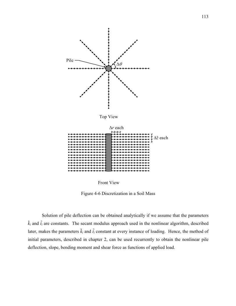
113
Top View
Pile Δθ
Front View
Δr each
Δz each
Figure 4-6 Discretization in a Soil Mass
Solution of pile deflection can be obtained analytically if we assume that the parameters
k i and t i are constants. The secant modulus approach used in the nonlinear algorithm, described
later, makes the parameters ki and t i constant at every instance of loading. Hence, the method of
initial parameters, described in chapter 2, can be used recurrently to obtain the nonlinear pile
deflection, slope, bending moment and shear force as functions of applied load.

114
4.5. Interdependence and Iterative Solutions of Pile and Soil Displacements
It is evident from equations (4-51) and (4-52) that the functions φr(r) and φθ(r) need to be
known to estimate the parameters ki and t i. This means that pile deflection cannot be obtained
unless φr(r) and φθ(r) are determined. In order to determine φr(r) and φθ(r), the quantities ms1,
ms2, ms3, ns1 and ns2 need to be known, which, in turn, depend on the pile deflection w and slope
dw dz . Therefore, the pile-deflection and the soil-displacement equations are coupled (similarly
to the linear elastic case of chapter 3), and have to be solved simultaneously using an iterative
scheme (note that this iteration is separate from the φ-iterations described before).
In order to solve the coupled equations, trial profiles for φr and φθ are assumed and the
values of ti and ki are obtained from equations (4-51) and (4-52) using numerical integration.
Pile deflection is then obtained using the method of initial parameters so that ms1, ms2, ms3, ns1
and ns2 can be determined. Using the calculated values of ms1, ms2, ms3, ns1 and ns2, φr and φθ are
determined by solving equations (4-33) and (4-34) (using φ-iterations). The newly obtained
profiles of φr and φθ are then compared with the previous (trial) profiles. If the differences are
within the tolerable limits of previous current 3
1
1 10m
j jr r
jmφ φ −
=
− ≤∑ and previous current 3
1
1 10m
j j
jmθ θφ φ −
=
− ≤∑ ,
then we accept the φr and φθ, and the corresponding w as the final solutions (note that the
convergence criterion of 10−3 is different from the convergence criterion of 10−8 for the φ-
iterations described before) . However, if the differences are greater than the tolerable limits,
then we assume the newly obtained profiles of φr and φθ as the new trial profiles for the next
iteration and repeat the process until convergence on both φr and φθ is achieved (we call this set
of iterations involving w, φr and φθ the w-iterations). The convergence criterion for the φ-
iterations is more stringent than that for the w-iterations because the φ-iterations are at the core of
this nonlinear analysis, and the accuracy of w, obtained from the w-iterations, depends on the
accuracy of φr and φθ obtained from the φ-iterations.
4.6. Nonlinear Algorithm
The nonlinear algorithm is fundamentally based on the concept of applying the external
load (or/and moment) (or a fraction thereof) and solve for pile deflection (through φ-iterations

115
and w-iterations) after obtaining the correct values of soil modulus based on the correct
displacement, strain and the stress fields, which are consistent with the applied loads.
Incremental load application is not necessary in this algorithm because the analysis is based on
secant modulus (ratio of total accumulated stress to corresponding strain) approach. If, for
example, the design load acting on the pile is Fa = 300 kN and Ma = 100kNm, the total load of
300 kN and 100 kNm can be applied in one step and pile deflection can be obtained. However,
if one needs to follow the progression of displacements as a function of the applied load (e.g., a
plot of head deflection versus applied load), then fractions of the total design load have to be
applied recurrently in increasing magnitudes (e.g., in the sequence of, say, 30 kN, 10 kNm; 60
kN, 20 kNm and so on) and the corresponding deflections have to be determined.
In order to start the algorithm, a small magnitude (say, 1 kN) of force (and/or moment) is
applied to determine the initial profiles of φr and φθ. For this “initial” load application, it is
assumed that the soil mass is homogeneous, isotropic and elastic within each layer. Thus, the
initial applied load has to be sufficiently small in order for the modulus to not degrade by any
significant amount such that the assumption of homogeneity with respect to soil modulus holds
good. For such an assumption, the analysis and algorithm developed in chapter 3 are valid, and
are used to obtain the initial pile deflection. For calculating the values of ki and ti for the initial
load application, the initial values of the elastic constants (Gs0 and υs0; or Gs0 and Ks0; or λs0 and
Gs0; or Es0 and υs0) are used. At the end of the initial load application, the profiles of φr and φθ
obtained from the initial load step are recorded for use as the initial trial profiles (φrini and φθini)
during the actual load application.
Next, the actual design load (or a fraction of it) is applied. Profiles of φrini and φθini are
used to calculate the strains using equation (3-3) at different points within the soil mass (the
values of pile deflection wi and slope idw dz obtained from the initial load application are used
in the calculation). Strains are calculated at the discrete points spaced at intervals of Δr and of
Δθ along the radial and circumferential directions, respectively (Figure 4-6). This discretization
is the same as described before for the calculation of k i and t i. Using the values of strains, the
elastic constants are calculated (by the use of an appropriate stress-strain relationship) at each of
the discretized points. From the calculated values of elastic constants and φrini and φθini at the

116
nodes, ti and k i are calculated using equations (4-51) and (4-52) (by the use of numerical
integration).
After the calculation of k i and ti, profiles of pile deflection and slope are obtained using
the method of initial parameters. Using these values, ms1, ms2, ms3, ns1 and ns2 are then calculated
from equations (4-26) through (4-29) and (4-32), respectively, using numerical integrations.
Here, the numerical integration (following the trapezoidal rule) is done along θ and z . For any
radial distance rj, integration along θ is first performed (with a step length of rjΔθ). The value of
the integral thus obtained is then used as the integrand to perform the integration along z with a
step length of Δz .
After obtaining ms1, ms2, ms3, ns1 and ns2, φr and φθ are determined by solving equations
(4-30b) and (4-31) using φ-iterations. Using the new values of φr,φθ, wi and idw dz , strains and
subsequently soil moduli are recalculated to again calculate ki and ti, which are then used to
calculate pile deflection. Iterations (w-iterations) are performed until the profiles of φr and φθ
between successive w-iterations match to the specified tolerable limits. Tolerance limits of
previous current 3
1
1 10m
j jr r
jmφ φ −
=
− ≤∑ and previous current 3
1
1 10m
j j
jmθ θφ φ −
=
− ≤∑ are used, which ensured proper
convergence. After the convergence is ensured, we get the pile deflection corresponding to the
applied load.
As mentioned before, the above solution scheme is valid for the full design load or a
fraction of it. If fractions of the design load are recurrently applied in increasing magnitudes to
determine how the pile deflection profile evolves with time, the same procedure has to be
repeated for each such load application. The nonlinear algorithm is outlined in Figure 4-7.

117
Figure 4-7 Nonlinear Solution Flow Chart
End
no
yes
no
no
yes
Normalize Input parameters: calculate aF , aM , iH
Choose initial guess for ( ) ( )old old1 1 2 2 = , = γ γ γ γ , …, ( )old
6 6 = γ γ
Calculate ki, ti
Calculate w , dwdz
for each layer using MIP
Calculate ( ) ( )new new1 1 2 2 = , = γ γ γ γ , …, ( )new
6 6 = γ γ
Apply initial load: (0)aF , (0)
aM
Input old new1 1
old new2 2
old new6 6
,
, ....,
γ γ
γ γ
γ γ
=
=
=
Check if old new1/ 2 / .../ 6 1/ 2 / ... / 6 0.001γ γ− <
Calculate φr and φθ using φ-iterations
Store φr and φθ as φrini and φθini
Input previousjrφ = φr
ini, previousjθφ = φθini
Apply actual load: ( )laF , ( )l
aM
Calculate ki, ti
Calculate w , dwdz
for each layer using MIP
Calculate ms1, ms2, ms3, ns1 and ns2
Calculate φr ( )currentjrφ=
and φθ ( )currentjθφ= using φ-iterations
Check if previous current 3
110
mj jr r
jφ φ −
=
− ≤∑and
previous current 3
110
mj j
jθ θφ φ −
=
− ≤∑
Input previous currentj j
r rφ φ= previous currentj j
θ θφ φ=
Calculate soil strain and modulus
Check if l < number of load
increment
Print w and other relevant quantities
log(γs)
Gs
Input Lp, rp, Ep, n, Hi, Fa, Ma,
number of load increment and
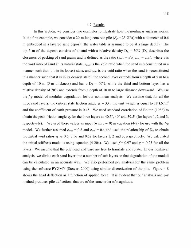
118
4.7. Results
In this section, we consider two examples to illustrate how the nonlinear analysis works.
In the first example, we consider a 20-m long concrete pile (Ep = 25 GPa) with a diameter of 0.6
m embedded in a layered sand deposit (the water table is assumed to be at a large depth). The
top 5 m of the deposit consists of a sand with a relative density DR = 50% (DR describes the
closeness of packing of sand grains and is defined as the ratio (emax − e)/( emax − emin), where e is
the void ratio of sand at its natural state, emax is the void ratio when the sand is reconstituted in a
manner such that it is in its loosest state, and emin is the void ratio when the sand is reconstituted
in a manner such that it is in its densest state), the second layer extends from a depth of 5 m to a
depth of 10 m (5-m thickness) and has a DR = 60%, while the third and bottom layer has a
relative density of 70% and extends from a depth of 10 m to large distance downward. We use
the f-g model of modulus degradation for our nonlinear analysis. We assume that, for all the
three sand layers, the critical state friction angle φc = 33°, the unit weight is equal to 18 kN/m3
and the coefficient of earth pressure is 0.45. We used standard correlation of Bolton (1986) to
obtain the peak friction angle φp for the three layers as 40.5°, 40° and 39.5° (for layers 1, 2 and 3,
respectively). We used these values as input (with c = 0) in equation (4-7) for use with the f-g
model. We further assumed emax = 0.8 and emin = 0.4 and used the relationship of DR to obtain
the initial void ratios e0 as 0.6, 0.56 and 0.52 for layers 1, 2 and 3, respectively. We calculated
the initial stiffness modulus using equation (4-20a). We used f = 0.97 and g = 0.23 for all the
layers. We assume that the pile head and base are free to translate and rotate. In our nonlinear
analysis, we divide each sand layer into a number of sub-layers so that degradation of the moduli
can be calculated in an accurate way. We also performed p-y analysis for the same problem
using the software PYGMY (Stewart 2000) using similar discretization of the pile. Figure 4-8
shows the head deflection as a function of applied force. It is evident that our analysis and p-y
method produces pile deflections that are of the same order of magnitude.

119
0 4 8 12
Pile Head Deflection (mm)
0
100
200
300
Forc
e, F
a (kN
)
Present Analysisp-y Method
Figure 4-8 Head Deflection as a Function of Applied Force for a Pile in Sand
Next, we consider a problem of a 15-m long concrete pile (Ep = 25 GPa) embedded in a
bed of clay underlain by sand. The water table is at the ground surface. The diameter of the pile
is 1.0 m and is free at both the head and base. A horizontal force acts at the head. The clay
deposit is assumed to be normally consolidated (with a coefficient of earth pressure of 0.45)
extending from the ground surface to a depth of 13 m. We assumed that the bulk unit weight of
clay is 16 kN/m3 and φc = 30° for both the layers. The sand layer, in which the pile base sits,
consists of sand with DR = 70%, φc = 33°, emax = 0.8 and emin = 0.4, for which we got φp = 40.5°
and e0 = 0.52. We used equation (4-20b) to calculate the initial shear modulus of clays and used
equation (4-20a) for sand. For a comparison with the p-y method, we considered the criteria for
“soft-clay” as prescribed by API (1993). For obtaining the initial shear modulus of the clay
layers, we assumed the values available for lower Cromer till, which belongs to the category of
soft clays (Chakraborty, T. and Salgado, R., personal communication) for inputs in equation (4-
20b): Cg = 150.0, ng = 0.3, eg = 2.17. In order to calculate the initial void ratio of clay e0 from
the existing mean effective stress σm and OCR, we used the following equation
01ln ln
OCRm
a
e NPσλ κ⎛ ⎞ ⎛ ⎞= − −⎜ ⎟ ⎜ ⎟
⎝ ⎠⎝ ⎠ (4-53)

120
where N = 0.47, λ = 0.063 and κ = 0.009. Using the above equation, e0 for clay was found to be
0.65, 0.58, 0.55 and 0.44 for the soil in the depth ranges 0 m to 3 m, 3 m to 6 m, 6 m to 9 m, and
9 m to 13 m, respectively. The undrained shear strength (cohesion) of clay su was calculated
using the following equation:
( )0.8OCR100
u c
v
s φσ
⎛ ⎞= ⎜ ⎟⎝ ⎠
(4-54)
where σv is the vertical effective stress at a depth. The values of su obtained for the clay layers
are 2.79 kPa, 8.34 kPa, 13.9 kPa and 19.5 kPa for the depth ranges of 0 m to 3 m, 3 m to 6 m, 6
m to 9 m and 9 m to 15 m, respectively. The value of su was given as input to the p-y analysis
(PYGMY) and also to equation (4-7) for use with the f-g model. We assumed f = 1 and g = 0.3
for clay in the analysis. Figure 4-9 shows the head deflection as a function of applied horizontal
force for our method and the p-y method. It is again evident that our analysis and p-y method
produced results that are of the same order of magnitude.
0 5 10 15 20 25
Pile Head Deflection (mm)
0
50
100
150
Forc
e, F
a (kN
)
Present Methodp-y Method
Figure 4-9 Head Deflection as a Function of Applied Force for a Pile in Sand

121
Finally, we consider the pile load test performed at the Orange County in Indiana. A
closed-ended steel pipe pile of diameter 356 mm and thickness 12.7 mm was embedded into the
ground to a depth of 17.4 m. The soil profile is described in Figure 4-10. The soil properties are
given in Table 4-1.
Organic Clay
Silty Sand
Clayey Sandy Silt
Silty/ Clayey Sand
Sandy Silty Clay
Silty/ Clayey Sand
Silty ClayClayey Silt
Silty Clay
Clayey Silt
Very Dense Silt
Silty Clay
26
24
22
20
18
16
14
12
10
8
6
4
2
0
60504030201006050403020100Soil layers
Depth(m)
qc from C1(MPa)
qc from C2(MPa)
Figure 4-10 Soil Profile at the Pile Load Test Site in Orange County, Indiana

122
Table 4-1 Soil Properties at the Pile Load Test Site in Orange County, Indiana
Layer No.
Depth (m)
wc (%)
LL (%)
PL (%)
PI (%)
Total Unit Weight (kN/m3)
DR (%) e0 Cc Cs
cv (m2/sec)
σ'vp (kPa)OCR φc
(deg)su
(kPa)
1 0-2.9 96 138 49 89 13.4 - 3.56 0.67 0.821.66E-06 - - - -
2 2.9-3.7 15 - - - 22* 78 - - - - - 31* -
3 3.7-5.7 19 18 10 8 21.6 - 0.47 0.11 0.032.45E-07 265 5.6 - 78
4 5.7-7.3 - - - - 22* 52 - - - - - - 29* -
5 7.3-7.8 - - - - 21* - - - - - - - - -
6 7.8-9.0 - - - - 22* 81 - - - - - - 29* -
7 9.0-10.2 25 37 18 19 20.1 - 0.73 0.19 0.036.82E-07 365 3.2 - 220
8 10.2-12.0 23 29 19 10 20.6 0.63 0.13 0.013.43E-06 265 1.9 - 320
9 12.0-14.5 15 21 12 9 21.9 - 0.45 0.10 0.015.30E-07 750 4.9 - 103
10 14.5-17 11 22 12 10 21.6 - 0.40 0.08 0.023.75E-07 365 2.0 - 292
11 17-18.4 - - - - 21* 95~100 - - - - - - 30* -
Note: wc = natural water content, e0 = initial void ratio, LL = liquid limit, PL = plastic limit, PI = plasticity index;. Cc = compression index; Cs = recompression index, cv = vertical coefficient of cosolidation; σ′vp = preconsolidation pressure, OCR = overconsolidation ratio, φc = critical state friction angle, su = undrained shear strength, DR = relative density. * These values are assumed.
For analysis, we assume alternate clay and sand layers (layers 1, 3, 5 and 7 are assumed
to be clay while layers 2, 4 and 6 are assumed to be sands). The seventh layer is assumed to
have properties that are approximately the average of the layers 7 through 10. The initial void
ratio assumed for all the layers is 0.5 except for the top layer which is assumed to have a void
ratio of 1.6. For clays, the parameters corresponding to those of lower Cromer till, described
above, are assumed for determining the initial shear modulus. The f-g model with f = 0.97 and g
= 0.23 is considered. Figure 4-11 shows the plot of the pile head deflection versus applied
horizontal load as obtained from the field experiment and the analysis. It is evident that the
analysis result matches reasonably well with the field result.
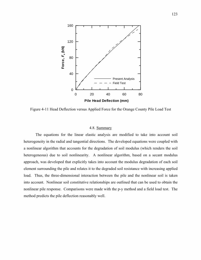
123
0 20 40 60 80
Pile Head Deflection (mm)
0
40
80
120
160
Forc
e, F
a (kN
)
Present AnalysisField Test
Figure 4-11 Head Deflection versus Applied Force for the Orange County Pile Load Test
4.8. Summary
The equations for the linear elastic analysis are modified to take into account soil
heterogeneity in the radial and tangential directions. The developed equations were coupled with
a nonlinear algorithm that accounts for the degradation of soil modulus (which renders the soil
heterogeneous) due to soil nonlinearity. A nonlinear algorithm, based on a secant modulus
approach, was developed that explicitly takes into account the modulus degradation of each soil
element surrounding the pile and relates it to the degraded soil resistance with increasing applied
load. Thus, the three-dimensional interaction between the pile and the nonlinear soil is taken
into account. Nonlinear soil constitutive relationships are outlined that can be used to obtain the
nonlinear pile response. Comparisons were made with the p-y method and a field load test. The
method predicts the pile deflection reasonably well.

124
CHAPTER 5. PILE GROUP ANALYSIS
5.1. Introduction
In this chapter, the interaction of piles embedded in a linear elastic continuum is studied.
The influence of one pile on any other in a group is modeled by modifying the soil resistance
which is assumed to be a function of the number of piles and their positions. The additional
displacement that a pile undergoes due to the loading of the other is captured.
5.2. Overview
Interactions between piles within a pile group play an important role in determining the
response of the group to external lateral loads. As a pile group is loaded, each pile pushes the soil
in the direction of the applied force and generates stresses in the soil mass. Each pile creates a
zone of influence within which the stresses caused by the pile are significant. Such zones of
influence of all the piles in a group overlap due to the close pile spacings (Figure 1-4). The
overlapping zones of influence of each pile not only transfer load to neighboring piles but also
cause a reduction in the soil stiffness between piles (Matlock et al 1980, Meimon et al. 1986,
Brown et al. 1987, McVay 1996).
The p-y method, modified to take into account the overall stiffness reduction of group
piles, is one of the most common methods of pile group analysis (Brown et al. 1988, 1987). In
this method, the soil resistance p is reduced by multiplying p by a factor f (called the p-
multiplier). The values of the p-multipliers are a function of spacing and position of the piles
(Reese et al. 2006). The multipliers have been back-calculated to match experimental and
numerical results (Brown and Shie 1991, Ruesta and Townsend 1997, Rollins et al. 1998, Zhang
et al. 1999b, Ng et al. 2001, Holloway et al. 1981, Baguelin et al. 1985, McVay et al. 1994, 1995,
1998, Ilyas et al. 2004).
Alternative approaches are also available based on the concept of beams on elastic
foundations. Ooi and Duncan (1994) and Ooi et al. (2004) addressed the issue of increase in

125
deflection by a group-amplification procedure, which is based on the characteristic load method
(Duncan et al. 1994). Davisson (1970), based on a subgrade-reaction analysis, proposed a
reduction in the values of the modulus of subgrade reaction for use in group analysis.
Dunnuvant and O’Neill (1986) proposed a reduction in stiffness of the piles depending on their
position in the group. Nogami and Paulson (1985) used a network of Winkler springs
interconnected to all the piles in the group and a transfer matrix to analyze the problem. Bogard
and Matlock (1983) replaced the actual piles within a group with an equivalent single pile
(applicable for closely-spaced piles) and developed equivalent p-y curves. They proposed a y-
multiplier concept (with multiplier values greater than one) to account for the excess deflection
of pile groups with respect to that of individual piles (applicable for groups with widely spaced
piles). Ashour et al. (2001) and (2004) applied the strain wedge model to analyze pile groups.
Several continuum-based approaches are also available. Poulos (1971b) pioneered the
continuum-based research by modifying his boundary integral technique, based on Mindlin’s
solution, to account for interaction between piles within groups. Many researchers have since
then used different forms of the boundary integral technique, including the boundary element
method, and have approximately accounted for soil nonlinearity and heterogeneity (Poulos 1975,
Banerjee 1978, Banerjee and Davies 1980, Sharnouby and Novak 1985, Basile 1999, Xu and
Poulos 2000). The finite element method, with several modifications (e.g., finite elements with
Fourier technique, finite elements with substructuring, finite elements with periodic boundary
conditions), has also been used quite extensively to model pile groups in elastic and elasto-
plastic soils (Chow 1987, Shibata et al. 1988, Kooijman 1989, Brown and Shie 1991, Bransby
1996, Zhang et al. 1999b, Wakai et al. 1999, Zhang and Small 2000, Law and Lam 2001,
Budiman and Ahn 2005). That apart, the discrete element method (Holloway et al. 1981), the
finite difference method (Comodromos and Pitilakis 2005) and the variational method (Shen and
Teh 2002) have been used to analyze pile groups.
A few mixed methods of analysis are also available, which are the combinations of the
continuum-based approach and the beam-on-foundation approach. Focht and Koch (1973)
combined the integral equation approach of Poulos (1971b) and the p-y method, assuming that
the deflection of a pile group depends both on the nonlinear soil behavior and on the pile-soil-
pile interaction. A similar hybrid model was developed by Leung and Chow (1987), who
modeled the soil response using the subgrade reaction method, and interaction between piles was

126
captured using Mindlin’s solution. Reese et al. (1984) modified the method of Focht and Koch
(1973) by calculating the elastic deflection from the linear portion of the p-y curves. O’Neill et
al. (1977) proposed a mixed method involving Mindlin’s solution and functional relationships
between load and deformations at the pile head, which were developed using the finite difference
method and cubic spline functions. Based on elastic interaction in a horizontal plane, Hariharan
and Kumarasamy (1983) obtained expressions for load and displacement multipliers for p-y
curves.
In this chapter, we propose coefficients f (Reese et al. 2006) to be multiplied with the soil
resistances ki and ti of the single-pile analysis (see chapter 4) to obtain the modified soil
resistances for pile groups. Thus, the single-pile analysis is modified to obtain the nonlinear
response of pile groups. We consider pile groups consisting of 2, 3, 4 and 6 piles.
5.3. Soil Resistance for Pile Groups
The two-pile-group problem can be described by Figure 5-1. For coefficient f to be used
for pile 1 and 2 are respectively given by: 0.26
120.7 1.02 p
rfr
⎛ ⎞= ≤⎜ ⎟⎜ ⎟
⎝ ⎠ (5-1)
0.38
120.48 1.02 p
rfr
⎛ ⎞= ≤⎜ ⎟⎜ ⎟
⎝ ⎠ (5-2)
where r12 is the center-to-center spacing between the two piles.
r12
x
y
Ma
Fa r02 1Pile
Pile cap
Figure 5-1 Two-Pile Group

127
The three-pile group can be described by Figure 5-2. The coefficient f for pile 1 can be
expressed as:
1 2f β β= (5-3)
with 0.26
121 0.7 1.0
2 p
rr
β⎛ ⎞
= ≤⎜ ⎟⎜ ⎟⎝ ⎠
(5-4)
0.26
12 232 0.7 1.0
2 p
r rr
β⎛ ⎞+
= ≤⎜ ⎟⎜ ⎟⎝ ⎠
(5-5)
For pile 2, equation (5-3) is valid with 0.26
231 0.7 1.0
2 p
rr
β⎛ ⎞
= ≤⎜ ⎟⎜ ⎟⎝ ⎠
(5-7)
0.38
122 0.48 1.0
2 p
rr
β⎛ ⎞
= ≤⎜ ⎟⎜ ⎟⎝ ⎠
(5-8)
For pile 3, equation (5-3) is valid with 0.38
231 0.48 1.0
2 p
rr
β⎛ ⎞
= ≤⎜ ⎟⎜ ⎟⎝ ⎠
(5-7)
0.38
12 232 0.48 1.0
2 p
r rr
β⎛ ⎞+
= ≤⎜ ⎟⎜ ⎟⎝ ⎠
(5-8)
r23 r12
r02 Fa
x
y
Ma3 1
Pile
Pile cap
Figure 5-2 Three-Pile Group
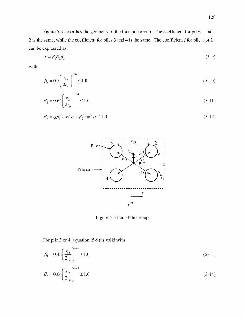
128
Figure 5-3 describes the geometry of the four-pile group. The coefficient for piles 1 and
2 is the same, while the coefficient for piles 3 and 4 is the same. The coefficient f for pile 1 or 2
can be expressed as:
1 2 3f β β β= (5-9)
with 0.26
231 0.7 1.0
2 p
rr
β⎛ ⎞
= ≤⎜ ⎟⎜ ⎟⎝ ⎠
(5-10)
0.34
122 0.64 1.0
2 p
rr
β⎛ ⎞
= ≤⎜ ⎟⎜ ⎟⎝ ⎠
(5-11)
2 2 2 23 1 2cos sin 1.0β β α β α= + ≤ (5-12)
α
α
2r23
r13
x
y
Ma
Fa
r0
3
1
Pile
Pile cap
4
r12
Figure 5-3 Four-Pile Group
For pile 3 or 4, equation (5-9) is valid with 0.38
231 0.48 1.0
2 p
rr
β⎛ ⎞
= ≤⎜ ⎟⎜ ⎟⎝ ⎠
(5-13)
0.34
122 0.64 1.0
2 p
rr
β⎛ ⎞
= ≤⎜ ⎟⎜ ⎟⎝ ⎠
(5-14)

129
2 2 2 23 1 2cos sin 1.0β β α β α= + ≤ (5-15)
The six-pile group is described by Figure 5-4. The factor f for pile 1 or 2 is given by
1 2 3 4 5f β β β β β= (5-16)
with 0.26
231 0.7 1.0
2 p
rr
β⎛ ⎞
= ≤⎜ ⎟⎜ ⎟⎝ ⎠
(5-17)
0.26
23 462 0.7 1.0
2 p
r rr
β⎛ ⎞+
= ≤⎜ ⎟⎜ ⎟⎝ ⎠
(5-18)
0.34
123 0.64 1.0
2 p
rr
β⎛ ⎞
= ≤⎜ ⎟⎜ ⎟⎝ ⎠
(5-19)
2 2 2 24 2 3cos sin 1.0β β δ β δ= + ≤ (5-20)
2 2 2 25 1 1 3 1cos sin 1.0β β α β α= + ≤ (5-21)
For pile 3 or 4, equation (5-16) is valid with 0.38
231 0.48 1.0
2 p
rr
β⎛ ⎞
= ≤⎜ ⎟⎜ ⎟⎝ ⎠
(5-22)
0.26
462 0.7 1.0
2 p
rr
β⎛ ⎞
= ≤⎜ ⎟⎜ ⎟⎝ ⎠
(5-23)
0.34
123 0.64 1.0
2 p
rr
β⎛ ⎞
= ≤⎜ ⎟⎜ ⎟⎝ ⎠
(5-24)
2 2 2 24 2 2 3 2cos sin 1.0β β α β α= + ≤ (5-25)
2 2 2 25 1 1 3 1cos sin 1.0β β α β α= + ≤ (5-26)
For pile 5 or 6, equation (5-16) is again valid with 0.38
23 461 0.48 1.0
2 p
r rr
β⎛ ⎞+
= ≤⎜ ⎟⎜ ⎟⎝ ⎠
(5-22)

130
0.38
462 0.48 1.0
2 p
rr
β⎛ ⎞
= ≤⎜ ⎟⎜ ⎟⎝ ⎠
(5-23)
0.34
123 0.64 1.0
2 p
rr
β⎛ ⎞
= ≤⎜ ⎟⎜ ⎟⎝ ⎠
(5-24)
2 2 2 24 2 2 3 2cos sin 1.0β β α β α= + ≤ (5-25)
2 2 2 25 1 3cos sin 1.0β β δ β δ= + ≤ (5-26)
r23
α2
4r46
r13
r25
x
y
6
3
Pile
Pile cap
5
α1
δ
2 r23
MaFa
r0
r12
1
r56
Figure 5-4 Four-Pile Group
5.4. Results
In order to illustrate the pile group analysis, we consider the soil profile of the example
problem of Figure 4-9 (clay layers overlain by a sand layer); however, instead of a single pile,
we assume a four-pile group with a center-to-center spacing of 2.5 m. All the piles in the group
are assumed to be 15 m long with diameters equal to 1.0 m. We restrain the rotation at the head
of all the piles with the assumption that the piles are attached to a rigid pile cap. Figure 5-5
shows the head deflections of the leading and trailing piles as a function of applied force. Also
plotted in the figure is the head deflection of a single pile (i.e., without a group) with a restrained
head condition that has the same length and diameter as those of the piles in the group. It is
evident that the leading pile has a slightly stiffer response than the trailing pile. In general, the

131
pile group deflects more than a single pile. For example, if we want to restrict the head
deflection at 10 mm, say, then the corresponding load at the head of the leading pile is 155 kN,
while that at the head of the trailing pile is 125 kN. Thus, a maximum total load of 2 × (155 +
125) = 560 kN can be applied on the group. In contrast, the maximum load that can be applied
for a 10 mm deflection for a single pile is 165 kN.
0 4 8 12 16 20
Pile Head Deflection (mm)
0
40
80
120
160
200
Forc
e, F
a (kN
)
Leading PileTrailing PileSingle Pile
Figure 5-5 Six-Pile Group
5.5. Summary
In this chapter, we propose a method for analysis of pile groups. The method is an
extension of the single pile analysis. Different coefficients (depending on the position of a pile
in a group and the number of piles in a group) are proposed that modify the soil resistances
obtained from single pile analysis for different pile groups. An example is provided to illustrate
the method.

132
CHAPTER 6. RETROSPECTION AND RECOMMENDATIONS
6.1. Introduction
In this final chapter, we present a summary of the research presented in the previous
chapters. We also present the main conclusions. Finally, we give recommendations for future
extensions of this research.
6.2. Summary
In this research study, we developed a continuum-based analysis of piles embedded in
multiple soil layers and subjected to a horizontal force and moment at the pile head. The pile is
modeled as an Euler-Bernoulli beam while the soil surrounding the pile is modeled as either a
linear elastic or a nonlinear elastic material. The displacements in the soil are described as
products of separable variables with different dimensionless shape functions for radial and
tangential displacements accounting for the decay in the soil displacements with increasing radial
distance from the pile. The differential equations governing the equilibrium configuration of the
pile-soil system were derived applying the principle of minimum potential energy. The
differential equation of pile deflection was solved analytically while the differential equations of
soil displacements were solved using the one-dimensional finite difference method. An iterative
solution algorithm was developed that ensured the global equilibrium of the pile-soil system.
The method takes into account the three-dimensional interaction of the pile with the surrounding
soil and produces pile response comparable with that from three-dimensional (3D) finite element
method (FEM); however, the computational effort required by the method is much less than that
required by an equivalent 3D FEM (nonlinear pile response is produced within minutes).
Analysis of pile group was also performed by modifying the soil resistance depending on the
number of piles in a group and the relative positions of the piles
In chapter 1, we presented a brief overview of piles foundations. We discussed the statics
and kinematics of pile response against vertical and lateral loads and discussed the soil spring

133
approach and the continuum approach of analysis of laterally loaded piles. We established that
the continuum approach is conceptually more appropriate for analysis of laterally loaded piles;
this set the stage for the analysis that was performed as a part of this research. In chapter 2, we
showed that a simple beam-on-elastic foundation approach can also be used to analyze laterally
loaded piles as a prologue to the continuum analysis subsequently performed. It revealed the
analogy between the soil-spring approach and the continuum approach. An analytical method of
solving differential equations, the method of initial parameters, was modified and applied to the
governing differential equation of pile deflection. In chapter 3, the continuum-based elastic
analysis for a single, circular pile was presented. The differential equations for pile deflection
and soil displacements were systematically developed using the principle of minimum potential
energy and calculus of variations. An iterative solution algorithm was used. The linear elastic
analysis was extended to take into account the soil nonlinearity in chapter 4. Different
constitutive models describing soil nonlinearity were first introduced and then the mathematical
analysis developed for linear soil was modified to produce the nonlinear pile response. Pile
groups were analyzed in chapter 5 by incorporating into the analysis modified soil resistance as a
function of the number of piles in a group and of the relative position of the piles.
Through this research, we have demonstrated that a complex three-dimensional boundary
value problem, that have so far been analyzed either by simple soil-spring approach or expensive
three-dimensional numerical analysis, can be solved with minimal computational effort yet
maintaining sufficient rigor so that the essential features of the pile-soil interaction are captured.
The need for representing soil resistance by springs with empirical spring constants (which, in
the case of nonlinearity, depend on pile deflection) is completely eliminated as the resistance is
rigorously calculated using integral equations that are functions of soil modulus and of the rate of
decrease of soil displacements with radial distance from the pile. The unique feature of this
analysis is that, along with the pile response (i.e., pile deflection, bending moment and shear
force), displacements and strains in the surrounding soil can also be obtained. Such a detailed
analysis has so far been possible only by the use of three-dimensional numerical analysis like the
finite element analysis, which is expensive and cannot be performed routinely for design. By the
use of this analysis, pile response is obtained semi-analytically in minutes and can be readily
used in design calculations. The inputs required for the analysis are pile geometry and modulus;
and the soil properties, typically the soil Poisson’s ratio, the void ratio, and the number and

134
thickness of soil layers, that can be determined from simple in situ or laboratory tests. The
inputs can be typed in a text file requiring minimum effort on the part of the user.
6.3. Future Research
Any new analysis method requires sufficient checks before it can be accepted in practice.
In the above research, the analysis has been compared with the exiting p-y method. However,
the p-y method cannot truly represent soil behavior, and moreover, the present analysis produces
soil displacements and strains along side pile deflection, which the p-y method cannot produce.
Thus, we need a systematic way of validating the analysis developed in the research, which will
check the pile deflections, and soil displacements and strains. An important point to note is that,
unlike the p-y method, the analysis uses soil parameters that can be estimated from routine tests.
Controlled pile load tests, in which soil properties are estimated using routine tests, is an
appropriate way to validate the analysis. That will help us to estimate the soil resistance with
reasonable accuracy, which is often not possible in real field problems due to inadequate site
characterization. Thus, we recommend the development of a load testing program. The Bowen
laboratory at Purdue University has the facility for performing laboratory-scale pile load tests
under controlled conditions. It is envisaged that the facility can be used successfully to develop
the testing program.

135
LIST OF REFERENCES
Aköz, Y., Öntuna, K. A. & Sağlamer, A. (1981). A new approach to the analysis of laterally loaded piles. Proc. 10th Int. Conf. Soil Mech. Fdn. Engng. 2, Stolkholm, 587-592. American Petroleum Institute. (1993). Recommended practice for planning, designing and constructing fixed offshore platforms – working stress design, API-RP-2A, 20th edition. Anagnostopoulos, C. & Georgiadis, M. (1993). Interaction of axial and lateral pile responses. Geotech. Engng., Am. Soc. Civ. Engrs. 119, No. 4, 793-798. Anderson, J. B. & Townsend, F. C. (2001). SPT and CPT testing for evaluating lateral loading of deep foundations. J. Geotech. Geoenv. Engng., Am. Soc. Civ. Engrs. 127, No. 11, 920-925. Anderson, J. B., Townsend, F. C. & Grajales, B. (2003). Case history evaluation of laterally loaded piles. J. Geotech. Geoenv. Engng., Am. Soc. Civ. Engrs. 129, No. 3, 187-196. Ashford, S. C. & Juirnarongrit, T. (2003). Evaluation of pile diameter effect on initial modulus of subgrade reaction. J. Geotech. Geoenv. Engng., Am. Soc. Civ. Engrs. 129, No. 3, 234-242. Ashour, M. & Norris, G. (2000). Modeling lateral soil-pile response based on soil-pile interaction. J. Geotech. Geoenv. Engng., Am. Soc. Civ. Engrs. 126, No. 5, 420-428. Ashour, M., Norris, G. & Pilling, P. (1998). Lateral loading of a pile in layered soil using the strain wedge model. J. Geotech. Geoenv. Engng., Am. Soc. Civ. Engrs. 124, No. 4, 303-315. Ashour, M., Pilling, P. & Norris, G. (2001). Assessment of pile group response under lateral load. Proc. 4th Int. Conf. Recent Advan. Geotech. Engng., San Diego, 1-6. Ashour, M., Pilling, P. & Norris, G. (2004). Lateral behavior of pile groups in layered soils. J. Geotech. Geoenv. Engng., Am. Soc. Civ. Engrs. 130, No. 6, 580-592. Baguelin, F., Frank, R. & Saĭd, Y. H. (1977). Theoretical study of lateral reaction mechanism of piles. Geotechnique 27, No. 3, 405-434. Banerjee, P. K. (1978). Analysis of axially and laterally loaded pile groups. Develop. Soil Mech., 1, Ed. Scott, C. R., Applied Science Pub. Ltd. Lond., 317-346. Banerjee, P. K. & Davies, T. G. (1978). The behavior of axially and laterally loaded single piles embedded in nonhomogeneous soils. Geotechnique 28, No. 3, 309-326.

136
Banerjee, P. K. & Davies, T. G. (1980). Analysis of some reported case histories of laterally loaded pile groups. Num. Meth. Offshore Piling, Inst. Civ. Engrs. 101-108. Basile, F. (1999). Non-linear analysis of pile groups. Proc. Instn. Civ. Engrs. Geotech. Engng. 137, 105-115. Basu, D. (2006). Analysis of laterally loaded piles in layered soil. Ph.D. Thesis, Purdue University. Basu, D. & Salgado, R. (2007a). Elastic analysis of laterally loaded pile in multi-layered soil. Geomech. Geongng. Int. J. 2, No. 3, 183-196. Basu, D. & Salgado, R. (2007b). Method of initial parameters for laterally loaded piles embedded in layered Soils. Geomech. Geongng. Int. J. 2, No. 4, 281-294. Bhowmik, S. K. & Long, J. H. (1991). An analytical investigation of the behavior of laterally loaded piles. Proc. Congress Geotech. Engng. Div. 2, Am. Soc. Civ. Engrs, 1307-1318. Biot, M. A. (1937). Bending of an infinite beam on an elastic foundation. J. Appl. Mech., Trans. Am. Soc. Mech. Engrs 4, No. 1, A1-A7. Block. H. D. (1962). Introduction to tensor analysis. Charles E. Merrill Books, Inc. Bogard, D & Matlock, H. (1983). Procedures for analysis of laterally loaded pile groups in soft clay. Proc. Geotech. Practice In Offshore Engng., Am. Soc. Civ. Engrs., Texas, 499-535. Bolton, M. D. (1986). Strength and dilatancy of sands. Geotechnique 36, No. 1, 65-78. Bowles, J. (1997). Foundation analysis and design. McGraw-Hill. Bowman, F. (1958). Introduction to Bessel functions. Dover Publications, Inc. Bransby, M. F. (1996). Difference between load-transfer relationships for laterally loaded pile groups: active p-y or passive p-δ. J. Geotech. Engng., Am. Soc. Civ. Engrs. 122, No. 12, 1015-1018. Bransby, M. F. (1999). Selection of p-y curves for the design of single laterally loaded piles. Int. J. Num. Anal. Meth. Geomech. 23, 1909-1926. Briaud, J.-L. (1997). Sallop: simple approach for lateral loads on piles. J. Geotech. Geoenv. Engng., Am. Soc. Civ. Engrs. 123, No. 10, 958-964. Broms, B. B. (1964a). Lateral resistance of piles in cohesive soils. J. Soil Mech. Fdn. Div., Am. Soc. Civ. Engrs. 90, No. SM2, 27-63.

137
Broms, B. B. (1964b). Lateral resistance of piles in cohesionless soils. J. Soil Mech. Fdn. Div., Am. Soc. Civ. Engrs. 90, No. SM3, 123-156. Broms, B. B. (1965). Design of laterally loaded piles. J. Soil Mech. Fdn. Div., Am. Soc. Civ. Engrs. 91, No. SM3, 79-99. Brown, D. A. & Kumar, M. (1989). P-y curves for laterally loaded piles derived from three-dimensional finite element model. Numer. Models Geomech. NUMOG III, Ed. Pietruszak, S. & Pande, G.N., Elsevier Applied Science, 683- 690. Brown, D. A. & Shie, C. F. (1991). Modification of p-y curves to account for group effects on laterally loaded piles. Proc. Congress Geotech. Engng. Div. 1, Am. Soc. Civ. Engrs., 479-489. Brown, D. A., Reese, L. C. & O’Neill, M. W. (1987). Cyclic lateral loading of a large-scale pile group. J. Geotech. Engng., Am. Soc. Civ. Engrs. 113, No. 11, 1326-1343. Brown, D. A., Morrison, C. & Reese, L. C. (1988). Lateral load behavior of pile group in sand. J. Geotech. Engng., Am. Soc. Civ. Engrs. 114, No. 11, 1261-1276. Brown, D. A., Hidden, S. A. & Zhang, S. (1994). Determination of P-Y curves using inclinometer data. Geotech. Test. J., GTJODJ, 17, No. 2, 150-158. Budhu, M. & Davies, T. G. (1988). Analysis of laterally loaded piles in soft clays. J. Geotech. Engng. Div., Am. Soc. Civ. Engrs. 114, No. 1, 21-39. Budiman, J. & Ahn, K. (2005). Effects of pile cap in single pile and lateral capacity of pile groups. Geo-Frontiers 2005, GSP 132, CD ROM. Chandrasekharaiah, D. S. & Debnath, L. (1994). Continuum Mechanics. Academic Press. Chapra, S. C. & Canale, R. P. (1998). Numerical methods for engineers. WCB/McGraw-Hill. Chow, Y. K. (1987). Axial and lateral response of pile groups embedded in nonhomogeneous soils. Int. J. Numer. Anal. Meth. Geomech. 11, 621-638. Comodromos, E. M. & Pitilakis, K. D. (2005). Response evaluation for horizontally loaded fixed-head pile groups using 3-D non-linear analysis. Int. J. Numer. Anal. Meth. Geomech. 29, 597-625. Cox, W. R., Dixon, D. A. & Murphy, B. S. (1984). Lateral-load tests on 25.4-mm (1-in.) diameter piles in very soft clay in side-by-side and in-line groups. Laterally Loaded Deep Fdns., ASTM STP 835, 122-139. Davies, T. G. & Budhu, M. (1986). Non-linear analysis of laterally loaded piles in heavily overconsolidated clays. Geotechnique 36, No. 4, 527-538.

138
Davis, R. O. & Selvadurai, A. P. S. (1996). Elasticity and geomechanics. Cambridge Univ. Press. Davis, R. O. & Selvadurai, A. P. S. (2002). Plasticity and geomechanics. Cambridge Univ. Press. Davisson, M. T. (1970). Lateral load capacity of piles. Highway Res. Rec. 333, 104-112. Davisson, M. T. & Gill, H. L. (1963). Laterally loaded piles in a layered soil system. J. Soil Mech. Fdn. Div., Am. Soc. Civ. Engrs. 89, No. SM3, 63-94. Desai, C. S. & Appel, G. C. (1976). 3-D analysis of laterally loaded structures. Num. Meth. Geomech., Am. Soc. Civ. Engrs. Ed. Desai, C.S., 2, 405-418. Duncan, M., Evans, L. T. & Ooi, P. S. K. (1994). Lateral load analysis of single piles and drilled shafts. J. Geotech. Engng., Am. Soc. Civ. Engrs. 120, No. 5, 1018-1033. Dunnuvant, T. W. & O’Neill, M. W. (1986). Evaluation of design-oriented methods for analysis of vertical pile groups subjected to lateral load. Proc. 3rd Intl. Conf. Num. Meth. Offshore Piling, Paris, 303-316. Einav, I. (2005). Energy and variational principles for piles in dissipative soil. Geotechnique 55, No. 7, 515-525. Fahey, M. & Carter, J. P. (1993). A finite element study of the pressuremeter test in sand using a nonlinear elastic plastic model. Can. Geotech. J. 30, 348-362. Feagin, L. B. (1935). Lateral pile-loading tests. Trans. Am. Soc. Civ. Engrs., 236-254. Fleming, W. G. K., Weltman, A. J., Randolph, M. F. & Elson, W. K. (1992). Blackie & Son Ltd. Focht, J. A. & Koch, K. J. (1973). Rational analysis of the lateral performance of offshore pile groups. Proc. 5th Offshore Tech. Conf. 2, Houston, Texas, 701-708. Francis, A. (1964). Analysis of pile groups with flexural resistance. J. Soil Mech. Fdn. Div., Am. Soc. Civ. Engrs. 90, No. SM3, 1-32. Fung, Y. C. (1994). A first course in continuum mechanics for physical and biological engineers and scientists. Prentice-Hall, Inc. Fung, Y. C. & Tong, P. (2001). Classical and computational solid mechanics. World Scientific Publishing Co. Pte. Ltd., Singapore. Gabr, M. A., Lunne, T. & Powell, J. J. (1994). P-y analysis of laterally loaded piles in clay using DMT. J. Geotech. Engng., Am. Soc. Civ. Engrs. 120, No. 5, 816-837. Gandhi, S. R. & Selvam, S. (1997). Group effect on driven piles under lateral load. J. Geotech. Geoenv. Engng., Am. Soc. Civ. Engrs. 123, No. 8, 702-709.

139
Georgiadis, M. (1983). Development of p-y curves for layered soils. Proc. Conf. Geotech. Pract. Offshore Engng., Am. Soc. Civ. Engrs. 536-545. Georgiadis, M. & Butterfield, R. (1982). Laterally loaded pile behavior. J. Geotech. Engng. Div., Am. Soc. Civ. Engrs. 108, No. GT1, 155-165. Georgiadis, M., Anagnostopoulos, C. & Saflekou, S. (1992). Centrifugal testing of laterally loaded piles in sand. Can. Geotech. J. 29, 208-216. Guo, W. D. & Lee, F. H. (2001). Load transfer approach for laterally loaded piles. Int. J. Numer. Anal. Meth. Geomech. 25, No. 11, 1101-1129. Hardin, B. O. (1978). The nature of stress-strain behavior for soils. Earthquake Engng. Soil Dyn., Am. Soc. Civ. Engrs. 1, 3-90. Hardin, B. O. & Black, W. L. (1966). Sand stiffness under various triaxial stresses. J. Soil Mech. Fdn. Div., Am. Soc. Civ. Engrs. 92, No. SM2, 27-42. Hardin, B. O. & Black, W. L. (1968). Vibration modulus of normally consolidated clay. J. Soil Mech. Fdn. Div., Am. Soc. Civ. Engrs. 94, No. SM2, 353-369. Hardin, B. O. & Drnevich, V. P. (1972). Shear modulus and damping in soils: design equations and curves. J. Soil Mech. Fdn. Div., Am. Soc. Civ. Engrs. 98, No. SM7, 667-692. Hariharan, M. & Kumarasamy, K. (1983). Analysis of pile groups subjected to lateral loads. Proc. 3rd Int. Conf. Behav. Meth. Offshore Struct., Massachusetts, 383-390. Harr, M. E., Davidson, J. L., Ho, D.-M., Pombo, L. E., Ramaswamy, S. V. & Rosner, J. C. (1969). Euler beams on a two parameter foundation model. J. Soil Mech. Fdn. Div., Am. Soc. Civ. Engrs 95, No. SM4, 933-948. Hetényi, M. (1946). Beams on elastic foundation. Univ. Michigan Press, Ann Arbor. Holloway, D. M., Moriwaki, Y., Stevens, J. B. & Perez, J. Y. (1981). Response of a pile group to combined axial and lateral loading. Proc. 10th Int. Conf. Soil Mech. Fdn. Engng., 2, Stockholm, 731-734. Horsnell, M. R., Aldridge, T. R. & Erbrich, C. E. (1990). Lateral group behavior of piles in offshore soil conditions. Proc. 22nd Offshore Tech. Conf., Houston, Texas, 417-424. Hsiao, J. K. & Kumar, S. (2005). Predicted and measured response of precast concrete piles under lateral load. Electronic J. Geot. Engrg. < http://www.ejge.com/2005/ppr0607/ppr0607.htm> (November 13, 2006). Hsiung, Y. (2003). Theoretical elastic-plastic solution for laterally loaded piles. J. Geotech. Geoenv. Engng., Am. Soc. Civ. Engrs. 129, No. 6, 475-480.

140
Hsiung, Y. & Chen, Y. (1997). Simplified method for analyzing laterally loaded single piles in clays. J. Geotech. Geoenv. Engng., Am. Soc. Civ. Engrs. 123, No. 11, 1018-1029. Hsiung, Y.-M., Chen, S.-S. & Chou, Y.-C. (2006). Analytical solution for piles supporting combined lateral loads. J. Geotech. Geoenv. Engng., Am. Soc. Civ. Engrs. 132, No. 10, 1315-1324. Huang, A-B, Hsueh, C-K, O’Neill, M. W., Chern, S. & Chen, C. (2001). Effects of construction on laterally loaded pile groups. J. Geotech. Geoenv. Engng., Am. Soc. Civ. Engrs. 127, No. 5, 385-397. Huangfu, F.-M., Wang, Y.-Q. & Zhang, J. (2003). Behavior of pile under combined axial and lateral loading. J. Harbin Inst. Tech. 35, No. 6. 743-746. Illyas, T., Leung, C. F., Chow, Y. K. & Budi, S. S. (2004). Centrifuge model study of laterally loaded pile groups in clay. J. Geotech. Geoenv. Engng., Am. Soc. Civ. Engrs. 130, No. 3, 274-283. Ishibashi, I. & Zhang, X. (1993). Unified dynamic shear moduli and damping ratios of sand and clay. Soils Fdns. 33, No. 1, 182-191. Ismael, N. F. & Klym, T. W. (1978). Behavior of rigid piers in layered cohesive soils. J. Geotech. Engng. Div., Am. Soc. Civ. Engrs 104, No. GT8, 1061-1074. Jones, R. & Xenophontos, J. (1977). The Vlasov foundation model. Int. J. Mech. Sci 19, 317-323. Kerr, A. D. (1964). Elastic and viscoelastic foundation models. J. Appl. Mech., Trans. Am. Soc. Mech. Engrs 31, No. 3, 491-498. Kim, J. B. & Brungraber, R. J. (1976). Full-scale lateral load tests of pile groups. J. Geotech. Engng. Div., Am. Soc. Civ. Engrs. 102, No. GT1, 87-105. Kim, T. K., Kim, N-K, Lee, W. J. & Kim, Y. S. (2004). Experimental load-transfer curves of laterally loaded piles in Nak-Dong river sand. J. Geotech. Geoenv. Engng., Am. Soc. Civ. Engrs. 130, No. 4, 416-425. Kondner, R. L. (1963). Hyperbolic stress-strain response: cohesive soils. J. Soil Mech. Fdn. Div., Am. Soc. Civ. Engrs. 89, No. SM1, 115-143. Kooijman, A. P. (1989). Comparison of an elastoplastic quasi three-dimensional model for laterally loaded piles with field tests. Numer. Models Geomech. NUMOG III, Ed. Pietruszak, S. & Pande, G.N., Elsevier Applied Science, 675- 682. Kooijman, A. P. & Vermeer, P. A. (1988). Elastoplastic analysis of laterally loaded piles. Proc. 6th Int. Conf. Num. Meth. Geomech., Innsbruck, Austria. 2, 1033-1042.

141
Langhaar, H. L. (1989). Energy methods in applied mechanics. Robert E. Krieger Publishing Co., Inc. Law, H. K. & Lam, I. P. (2001). Application of periodic boundary for large pile group. J. Geotech. Geoenv. Engng., Am. Soc. Civ. Engrs. 127, No. 10, 889-892. Lee, J. & Salgado, R. (2000). Analysis of calibration chamber plate load tests. Can. Geotech. J. 37, 14-25. Lee, C. Y. & Small, J. C. (1991). Finite layer analysis of laterally loaded piles in cross-anisotropic soils. Int. J. Numer. Anal. Meth. Geomech. 15, 785-808. Lee, S. L., Kog, Y. C. & Karunaratne, G. P. (1987). Laterally loaded piles in layered soil. Soils Fdns. 27, No. 4, 1-10. Leung, C. F. & Chow, Y. K. (1987). Response of pile groups subjected to lateral loads. Int. J. Numer. Anal. Meth. Geomech. 11, 307-314. Loukidis, D. (2006).Advanced constitutive modeling of sands and applications to foundation engineering. Ph.D. Thesis, Purdue University. Lubliner, J. (1990). Plasticity theory. Macmillan Publishing Company. Madhav, M. R., Rao, N. S. V. K. & Madhavan, K. (1971). Laterally loaded pile in elasto-plastic soil. Soils Fdns. 11, No. 2, 1-15. Maharaj, D. K. (2003) Load-Deflection Response of Laterally Loaded Single Pile by Nonlinear Finite Element Analysis. Electronic J. Geot. Engrg. < http://www.ejge.com/2003/ppr0342/ppr0342.htm> (November 13, 2006). Mal, A. K. & Singh, S. J. (1991). Deformation of elastic solids. Prentice-Hall, Inc. Malvern, L. E. (1969). Introduction to the mechanics of a continuous medium. Prentice-Hall, Inc. Matlock, H. (1970). Correlations for design of laterally loaded piles in soft clay. Proc. 2nd Offshore Tech. Conf., Houston, Texas, 1, 577-594. Matlock, H. & Reese, L. C. (1960). Generalized solutions for laterally loaded piles. J. Soil Mech. Fdn. Div., Am. Soc. Civ. Engrs. 86, No. SM5, 63-91. Mayne, P. W. (2000). Enhanced Geotechnical Site Characterizatin by Seismic Piezocone Penetration Tests. Proc. 4th Int. Geot. Conf., Cairo University, 95-120. <http://www.geotechlinks.com/download.php?id=GL0138> (December 1, 2006). McClelland, B. & Focht Jr., J. A. (1958). Soil modulus for laterally loaded piles. Trans. Am. Soc. Civ. Engrs. 123, 1049-1063.
142
McLachlan, N. W. (1961). Bessel functions for engineers. Oxford Univ. Press. McVay, M., Casper, R. & Shang, T. I. (1995). Lateral response of three-row groups in loose to dense sands at 3D and 5D pile spacing. J. Geotech. Engng., Am. Soc. Civ. Engrs. 121, No. 5, 436-441. McVay, M., Bloomquist, D., Vanderlinde, D. & Clausen, J. (1994). Centrifuge modeling of laterally loaded pile groups in sands. Geotech. Test. J. GTJODJ, 17, No. 2, 129-137. McVay, M. C., Shang, T. I. & Casper, R. (1996). Centrifuge testing of fixed-head laterally loaded battered and plumb pile groups in sand. Geotech. Test. J. GTJODJ, 19, No. 1, 41-50. McVay, M., Zhang, L., Molnit, T. & Lai, P. (1998). Centrifuge testing of large laterally loaded pile groups in sands. J. Geotech. Geoenv. Engng., Am. Soc. Civ. Engrs. 124, No. 10, 1016-1026. Mindlin, R. D. (1936). Force at a point in the interior of a semi-infinite solid. Physics 7, May, 195-202. Mokwa, R. L. (1999). “Investigation of the resistance of pile caps to lateral loading.” Ph.D.
Thesis, Virginia Polytechnic Institute and State University.
Mokwa, R. L. & Duncan, J. M. (2001). Experimental evaluation of lateral-load resistance of pile caps. J. Geotech. Geoenv. Engng., Am. Soc. Civ. Engrs. 127, No. 2, 185-192. Naylor, D. J., Pande, G. N., Simpson, B. & Tabb, R. (1981). Finite elements in geotechnical engineering. Pineridge Press Ltd., Swansea, U. K. Ng, C. W. W., Rigby, D. B. Ng, S. W. L. & Lei, G. H. (2000). Field studies of well-instrumented barrette in Hong Kong. J. Geotech. Geoenv. Engng., Am. Soc. Civ. Engrs. 126, No. 1, 60-73. Ng C. W. W., Zhang, L. & Nip, D. C. N. (2001). Response of laboratory loaded large-diameter bored pile groups. J. Geotech. Geoenv. Engng., Am. Soc. Civ. Engrs. 127, No. 8, 658-669. Nogami, T. & Paulson, S. K. (1985). Transfer matrix approach for nonlinear pile group response analysis. Int. J. Numer. Anal. Meth. Geomech. 9, 299-316. O’Neill, M. W. & Murchinson, J. M. (1983). An evaluation of p-y relationships in sand. Rep. prepared for American Petroleum Inst., Washington, D.C. (as cited in Kim et al. 2004). O’Neill, M. W., Ghazzaly, O. I. & Ha, H. B. (1977). Analysis of three-dimensional pile groups with non-linear soil response and pile-soil-pile interaction. Proc. 9th Offshore Tech. Conf., Houston, Texas, 2, 245-256. O’Neill, M. W., Reese, L. C. & Cox, W. R. (1990). Soil behavior for piles under lateral loading. Proc. 22nd Offshore Tech. Conf., Houston, Texas, 3, 279-287.

143
Ooi, P. S. K. & Duncan, J. M. (1994). Lateral load analysis of groups of piles and drilled shafts. J. Geotech. Engng., Am. Soc. Civ. Engrs. 120, No. 6, 1034-1050. Ooi, P. S. K., Chang, B. K. F. & Wang, S. (2004). Simplified lateral load analyses of fixed-head piles and pile groups. J. Geotech. Geoenv. Engng., Am. Soc. Civ. Engrs. 130, No. 11, 1140-1151. Pile Buck. (2003). The pile driving, foundation and marine contractor’s newspaper. April. < http://www.pilebuck.com/newspaper/> (November 13, 2006). Pise, P. J. (1982). Laterally loaded piles in a two-layer soil system. J. Geotech. Engng. Div., Am. Soc. Civ. Engrs. 108, No. GT9, 1177-1181. Poulos, H. G. (1971a). Behavior of laterally loaded piles: I – single piles. J. Soil Mech. Fdn Div., Am. Soc. Civ. Engrs. 97, No. SM5, 711-731. Poulos, H. G. (1971b). Behavior of laterally loaded piles: II – pile groups. J. Soil Mech. Fdn Div., Am. Soc. Civ. Engrs. 97, No. SM5, 733-751. Poulos, H. G. (1972). Behavior of laterally loaded piles: III – socketed piles. J. Soil Mech. Fdn Div., Am. Soc. Civ. Engrs. 98, No. SM4, 341-360. Poulos, H. G. (1973). Load-deflection prediction for laterally loaded piles. Aust. Geomech. J. G3, No. 1, 1-8. Poulos, H. G. (1975) Lateral load-deflection prediction for pile groups. J. Geotech. Engng. Div., Am. Soc. Civ. Engrs. 101, No. GT1, 19-34. Poulos, H. G. & Davis, E. H. (1980). Pile foundation analysis and design. John Wiley & Sons, Inc. Prakash, S. & Sharma, H. D. (1990). Pile foundations in engineering practice. John Wiley & Sons, Inc. Pyke, R. & Beikae, M. (1984). A new solution for the resistance of single piles to lateral loading. Laterally Loaded Deep Fdns., ASTM STP 835, 3-20. Qiu, T., Fox, P. J., Janoyan, K., Stewart, J. P. & Wallace, J. W. (2004). Geo-Support 2004, Drilled Shafts, Micropiling, Deep Mixing, Remedial Methods, and Specialty Foundation Systems, GSP 124, 613-624. Randolph, M. F. (1981). The response of flexible piles to lateral loading. Geotechnique 31, No. 2, 247-259. Rao, N. S. V. K. (1998). Vibration analysis and foundation dynamics. Wheeler Publishing, New Delhi, India.

144
Rao, N. S. V. K., Das, Y. C. & Anandakrishnan, M. (1971). Variational approach to beams on elastic foundations. J. Engng. Mech. Div., Am. Soc. Civ. Engrs. 97, No. EM2, 271-294. Rao, S. N., Ramakrishna, V. G. S. T. & Rao, M. B. (1998). Influence of rigidity on laterally loaded pile groups in marine clay. J. Geotech. Geoenv. Engng., Am. Soc. Civ. Engrs. 124, No. 6, 542-549. Reddy, J. N. (2002). Energy principles and variational methods in applied mechanics. John Wiley & Sons, Inc. Reddy, A. S. & Valsangkar, A. J. (1970). Generalized solutions for laterally loaded pile in elasto-plastic soil. Soils Fdns. X, No. 3, 66-80. Reddy, A. S. & Valsangkar, A. J. (1971). Analysis of a laterally loaded pile in a layered soil by energy method. Acta Technica Academiae Scientiarum Hungaricae, Tomus 70 (1-2), 235-249. Reese, L. C. (1977). Laterally loaded piles: program documentation. J. Geotech. Engng. Div., Am. Soc. Civ. Engrs. 103, No. GT4, 287-305. Reese, L. C. (1997). Analysis of laterally loaded piles in weak rock. J. Geotech. Geoenv. Engng., Am. Soc. Civ. Engrs. 123, No. 11, 1010-1017. Reese, L. C. & Cox, W. R. (1969). Soil behavior from analysis of tests of uninstrumented piles under lateral loading. Performance of Deep Fdns., ASTM STP 444, 160-176. Reese, L. C. & Matlock, H. (1956). Non-dimensional solutions for laterally loaded piles with soil modulus assumed proportional to depth. Proc. 8th Texas Conf. on Soil Mech. Fdn. Engng., Austin, Texas, 1-41. Reese, J. C. & Van Impe, W. F. (2001). Single piles and pile groups under lateral loadings. A. A. Balkema, Rotterdam. Reese, L. C. & Welch, R. C. (1975). Lateral loading of deep foundations in stiff clay. J. Geotech. Engng. Div., Am. Soc. Civ. Engrs. 101, No. GT7, 633-649. Reese, L. C., Cox, W. R. & Koop, F. D. (1974). Analysis of laterally loaded piles in sand. Proc. 6th Offshore Tech. Conf., Houston, Texas, 2, 473-483. Reese, L. C., Wright, S. G. & Aurora, R. P. (1984). Analysis of a pile group under lateral loading. Laterally Loaded Deep Fdns., ASTM STP 835, 56-71. Reese, L. C., Cox, W. R. & Koop, F. D. (1975). Field testing and analysis of laterally loaded piles in stiff clay. Proc. 7th Offshore Tech. Conf., Houston, Texas, 2, 671-690. Reese, L. C., Isenhower, W. M. & Wang, S.-T. (2006). Analysis and design of shallow and deep foundations. John Wiley & Sons, Inc.

145
Rollins, K. M. & Sparks, A. (2002). Lateral resistance of full-scale pile cap with gravel backfill. J. Geotech. Geoenv. Engng., Am. Soc. Civ. Engrs. 128, No. 9, 711-723. Rollins, K. M., Peterson, K. T. &Weaver, T. J. (1998). Lateral load behavior of full-scale pile group in clay. J. Geotech. Geoenv. Engng., Am. Soc. Civ. Engrs. 124, No. 6, 468-478. Ruesta, P. F. & Townsend, F. C. (1997). Evaluation of laterally loaded pile group at Roosevelt bridge. J. Geotech. Geoenv. Engng., Am. Soc. Civ. Engrs. 123, No. 12, 1153-1161. Salgado, R. (2008). The engineering of foundations. The McGraw-Hill Companies, Inc. Scott, R. F. (1981). Foundation analysis. Prentice-Hall, Inc. Selvadurai, A. P. S. (1979). Elastic analysis of soil-foundation interaction, Elsevier Scientific Publishing Company. Sharnouby, B. E. & Novak, M. (1985). Static and low-frequency response of pile groups. Can. Geotech. J. 22, 79-94. Shen, W. Y. & Teh, C. I. (2002). Analysis of laterally loaded pile groups using variational approach. Geotechnique 52, No. 3, 201-208. Shen, W. Y. & Teh, C. I. (2004). Analysis of laterally loaded piles in soil with stiffness increasing with depth. J. Geotech. Geoenv. Engng., Am. Soc. Civ. Engrs. 130, No. 8, 878-882. Shibata, T, Yashima, A., Kimura, M. & Fukada, H. (1988). Analysis of laterally loaded piles by quasi-three-dimensional finite element method. Proc. 6th Intl. Conf. Numer. Meth. Geomech., Innsbruck, 1051-1058. Shibuya, S., Tatsuoka, F., Teachavorasinskun, S. Kong, X. J. Abe, F., Kim, Y.-S. & Park, C.-K. (1992). Elastic deformation properties of geomaterials. Soils Fdns. 32, No. 3, 26-46. Sogge, R. L. (1981). Laterally loaded pile design. J. Geotech. Engng. Div., Am. Soc. Civ. Engrs 107, No. GT9, 1179-1199. Stewart, D. P. (2000). User Manual PYGMY. Univ. West. Aust. Strang, G. (1988). Linear algebra and its applications. Thomson Learning, Inc. Sun, K. (1993). Static analysis of laterally loaded piles. Proc. 11th Southeast Asian Geotech. Conf., Singapore, 589-594. Sun, K. (1994a). Laterally loaded piles in elastic media. J. Geotech. Engng., Am. Soc. Civ. Engrs. 120, No. 8, 1324-1344. Sun, K. (1994b). A numerical method for laterally loaded piles. Comput. Geotech. 16, 263-289.

146
Terzaghi, K. (1955). Evaluation of coefficients of subgrade reaction. Geotechnique 5, No. 4, 297-326. Tomlinson, M. J. (1994). Pile design and construction practice. E & FN Spon. Trochanis, A. M., Bielak, J. & Christiano, P. (1991). Three-dimensional nonlinear study of piles. J. Geotech. Engng., Am. Soc. Civ. Engrs 117, No. 3, 429-447. Vallabhan, C. V. G. (1999). Validity of the Reese model for pile foundations using variational principles. Anal. Des. Const. Testing Deep Fdns., Geotech. Sp. Publ. 88, Am. Soc. Civ. Engrs., 61-75. Vallabhan, C. V. G. & Das, Y. C. (1988). Parametric study of beams on elastic foundations. J. Engng. Mech., Am. Soc. Civ. Engrs 114, No. 12, 2072-2082. Vallabhan, C. V. G. & Das, Y. C. (1991). Modified Vlasov model for beams on elastic foundations. J. Geotech. Engng., Am. Soc. Civ. Engrs 117, No. 6, 956-966. Valsangkar, A. J., Rao, N. S. V. K. & Basudhar, P. K. (1973). Generalized solutions of axially and laterally loaded piles in elasto-plastic soil. Soils Fdns. 13, No. 4, 1-14. Veruijt, A. & Kooijman, A. P. (1989). Laterally loaded piles in a layered elastic medium. Geotechnique 39, No. 1, 39-46. Vesić, A. B. (1961). Bending of beams resting on isotropic elastic solid. J. Engng. Mech. Div., Am. Soc. Civ. Engrs. 87, No. EM2, 35-53. Viggiani, G. & Atkinson, J. H. (1995). Stiffness of fine-grained soil at very small strains. Geotechnique 45, No. 2, 249-265. Vlasov, V. Z. & Leont’ev, N. N. (1966). Beams, plates and shells on elastic foundations. Israel Program for Scientific Translations, Jerusalem. Wakai, A, Gose, S. & Ugai, K. (1999). 3-D elasto-plastic finite element analysis of pile foundations subjected to lateral loading. Soils Fdns. 39, No. 1, 97-111. Wesselink, B. D., Murff, J. D., Randolph, M. F. Numez, I. L. & Hyden, A. M. (1988). Analysis of centrifuge model test data from laterally loaded piles in calcareous sand. Engineering for calcareous sediments, 1, Balkema, Rotterdam, 261-170. Winkler, E. (1867). Die Lehre von der Elasticitaet und Festigkeit, Prag, Dominicus. Wu, D., Broms, B. B. & Choa, V. (1998). Design of laterally loaded piles in cohesive soils using p-y curves. Soils Fdns. 38, No. 2, 17-26.

147
Xu, K. J. & Poulos, H. G. (2000). General elastic analysis of piles and pile groups. Int. J. Numer. Anal. Meth. Geomech. 24, 1109-1138. Yan, L. & Byrne, P. M. (1992). Lateral pile response to monotonic pile head loading. Can. Geotech. J. 29, 955-970. Yang, K. & Liang, R. (2006). Numerical solution for laterally loaded piles in a two-layer soil profile. J. Geotech. Geoenv. Engng., Am. Soc. Civ. Engrs. 132, No. 11, 1436-1443. Yang, C. C., Lin, S.-S., Juang, C. H. & Lee, W. F. (2002). Analysis of laterally loaded piles in a two-layered elastic medium. Deep Fdns. 2002 1, Am. Soc. Civ. Engrs., GSP 116, 80-93. Zhang, L. M. (2003). Behavior of laterally loaded large-section barrettes. J. Geotech. Geoenv. Engng., Am. Soc. Civ. Engrs. 129, No. 7, 639-648. Zhang, H. H. & Small, J. C. (2000). Analysis of capped pile groups subjected to horizontal and vertical loads. Comput. Geotech. 26, 1-21. Zhang, L., McVay, M. C. & Lai, P. W. (1999a). Centrifuge modelling of laterally loaded single battered piles in sands. Can. Geotech. J. 36, 1074-1084. Zhang, L., McVay, M. C. & Lai, P. (1999b). Numerical analysis of laterally loaded 3×3 to 7×3 pile groups in sands. J. Geotech. Geoenv. Engng., Am. Soc. Civ. Engrs. 125, No. 11, 936-946. Zhang, L., Ernst, H. & Einstein, H. H. (2000). Nonlinear analysis of laterally loaded rock-socketed shafts. J. Geotech. Geoenv. Engng., Am. Soc. Civ. Engrs 126, No. 11, 955-968. Zhang, L., Silva, F. & Grismala, R. (2005). Ultimate lateral resistance to piles in cohesionless soils. J. Geotech. Geoenv. Engng., Am. Soc. Civ. Engrs. 131, No. 1, 78-83. Zhaohua, F. & Cook, R. D. (1983). Beam elements on two-parameter elastic foundations. J. Engng. Mech., Am. Soc. Civ. Engrs. 109, No. 6, 1390-1402.