1

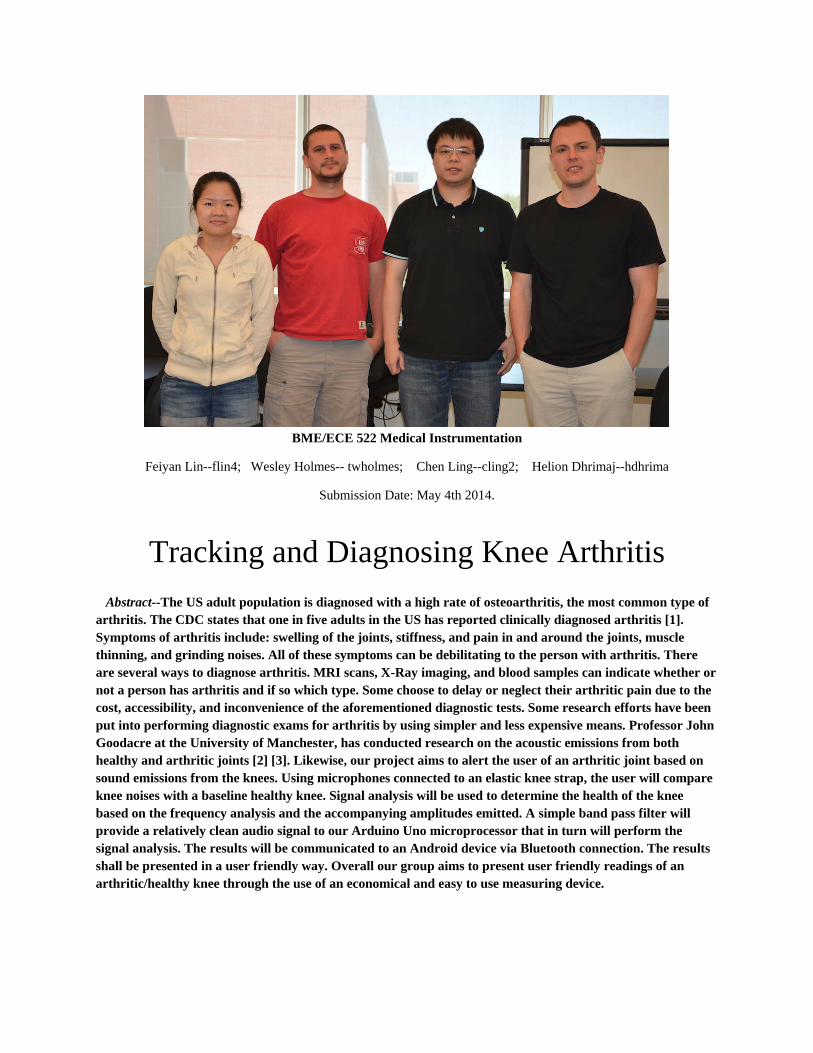
BME/ECE 522 Medical Instrumentation

Feiyan Lin--flin4; Wesley Holmes-- twholmes; Chen Ling--cling2; Helion Dhrimaj--hdhrima

Submission Date: May 4th 2014.

Tracking and Diagnosing Knee Arthritis

Abstract--The US adult population is diagnosed with a high rate of osteoarthritis, the most common type of arthritis. The CDC states that one in five adults in the US has reported clinically diagnosed arthritis [1]. Symptoms of arthritis include: swelling of the joints, stiffness, and pain in and around the joints, muscle thinning, and grinding noises. All of these symptoms can be debilitating to the person with arthritis. There are several ways to diagnose arthritis. MRI scans, X-Ray imaging, and blood samples can indicate whether or not a person has arthritis and if so which type. Some choose to delay or neglect their arthritic pain due to the cost, accessibility, and inconvenience of the aforementioned diagnostic tests. Some research efforts have been put into performing diagnostic exams for arthritis by using simpler and less expensive means. Professor John Goodacre at the University of Manchester, has conducted research on the acoustic emissions from both healthy and arthritic joints [2] [3]. Likewise, our project aims to alert the user of an arthritic joint based on sound emissions from the knees. Using microphones connected to an elastic knee strap, the user will compare knee noises with a baseline healthy knee. Signal analysis will be used to determine the health of the knee based on the frequency analysis and the accompanying amplitudes emitted. A simple band pass filter will provide a relatively clean audio signal to our Arduino Uno microprocessor that in turn will perform the signal analysis. The results will be communicated to an Android device via Bluetooth connection. The results shall be presented in a user friendly way. Overall our group aims to present user friendly readings of an arthritic/healthy knee through the use of an economical and easy to use measuring device.

2

Table of Contents: I. Background …………………………………………………………………………………….. 3 II. Statement of Problem …………………………………………………………………………. 4 III. Concept Development …………………………………………………………………….….. 4 Technical Specification ……………………………………………………………………….. 5 IV. Design Procedure …………………………………………………………………………....... 5 Band-Pass Filter Design ……………………………………………………………………… 6 Microprocessor (Arduino Uno) ……………………………………………………………… 14 Bluetooth TX/RX ……………………………………………………………………………... 14 Android Interface …………………………………………………………………………...... 17 V. Simulation Results ……………………………………………………………………………… 24 VI. Prototyping …………………………………………………………………………………….. 27 VII. Experimental Results ……………………………………………………………………….... 29 VIII. Conclusion ………………………………………………………………………………….... 35 Obstacles during the Process ………………………………………………………………… 35 Further Improvements ……………………………………………………………………….. 35 References ………………………………………………………………………………………….. 37 Appendix A: Microphone Data Sheet …………………………………………………………….. 38 Appendix B: Arduino Uno Data Sheet …………………………………………………………… 40 Appendix C: Op-Amp Data Sheet ………………………………………………………………… 41 Appendix D1: FHT Example Code for Arduino UNO …………………………………………… 42 Appendix D2: FTH Team Arthritis Code for Arduino UNO …………………………………… 43 Appendix D3: Livestream Arduino UNO Code…………………………………………………… 47 Appendix E1: MATLAB Spectrum Display Code………………………………………………… 48 Appendix E2: MATLAB Livestream Code………………………………………………………… 50

3

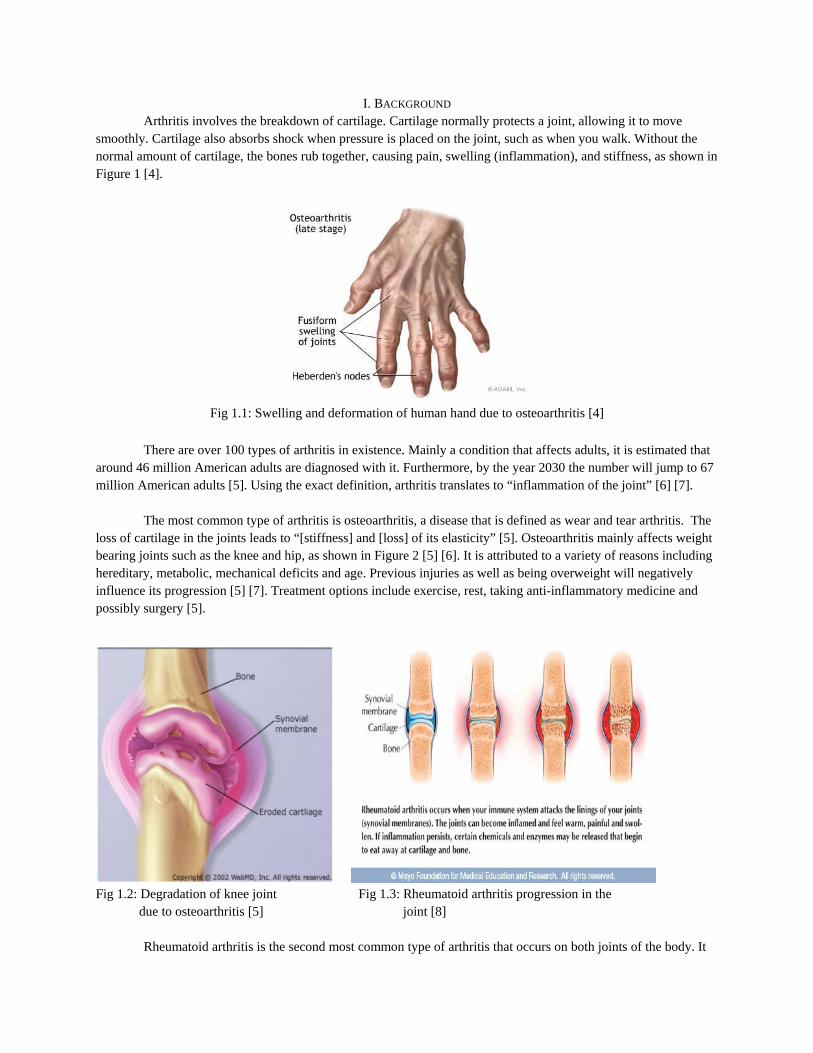
I. BACKGROUND Arthritis involves the breakdown of cartilage. Cartilage normally protects a joint, allowing it to move

smoothly. Cartilage also absorbs shock when pressure is placed on the joint, such as when you walk. Without the normal amount of cartilage, the bones rub together, causing pain, swelling (inflammation), and stiffness, as shown in Figure 1 [4].

Fig 1.1: Swelling and deformation of human hand due to osteoarthritis [4]

There are over 100 types of arthritis in existence. Mainly a condition that affects adults, it is estimated that

around 46 million American adults are diagnosed with it. Furthermore, by the year 2030 the number will jump to 67 million American adults [5]. Using the exact definition, arthritis translates to “inflammation of the joint” [6] [7]. The most common type of arthritis is osteoarthritis, a disease that is defined as wear and tear arthritis. The loss of cartilage in the joints leads to “[stiffness] and [loss] of its elasticity” [5]. Osteoarthritis mainly affects weight bearing joints such as the knee and hip, as shown in Figure 2 [5] [6]. It is attributed to a variety of reasons including hereditary, metabolic, mechanical deficits and age. Previous injuries as well as being overweight will negatively influence its progression [5] [7]. Treatment options include exercise, rest, taking anti-inflammatory medicine and possibly surgery [5].

Fig 1.2: Degradation of knee joint Fig 1.3: Rheumatoid arthritis progression in the due to osteoarthritis [5] joint [8]

Rheumatoid arthritis is the second most common type of arthritis that occurs on both joints of the body. It

4

is caused by the body attacking its own soft tissue and joints. It is thought to be a combination of different factors including genetic and hormonal factors [5] [6]. The progression of rheumatoid arthritis is shown in Figure 3. Symptoms of rheumatoid arthritis develop gradually, and it is generally considered a chronic disease. Most commonly, smaller joints such as hand and feet are affected but it can also affect larger parts [7]. Depending on factors such as age and medical history, treatments for rheumatoid arthritis include rest, exercise, medicine, and surgery.

A third type of arthritis is called gout arthritis, a disease which is caused by too much uric acid in the blood [5]. The joints become quite swollen and may lose their ability to function properly [7]. Being overweight and consuming too much alcohol are some of the factors which contribute to the onset of gout. Treatment of gout includes corticosteroids shots, anti-inflammatory as well as prescription medicine to decrease levels of uric acid. A moderate consumption of meats and alcohol will also help alleviate the symptoms [5].

II. STATEMENT OF PROBLEM Among all different types of arthritis, osteoarthritis is the most common type. Currently, diagnosis of

osteoarthritis is performed by doctors. The doctors start by conducting a physical exam and asking for the patients’ medical history. If the doctor suspects the possibility of osteoarthritis, he or she will order laboratory tests, x-ray or MRI scans. The diagnosis of osteoarthritis is not based on a single symptom or test result but rather on a combination of symptoms and test results to rule out other types of arthritis. Due to the number of tests that need to be performed, diagnosis of arthritis can be an arduous process.

After evaluating current market, there are no portable or less expensive equipment that can detect abnormal joint conditions not to mention diagnose osteoarthritis. This is inconvenient for individuals who want to avoid the trouble and cost of going to a doctor for just a simple test. Presented in this project, is a relatively cost-effective device and corresponding software that allows a consumer to collect data on his or her own knee joint and determine whether it is necessary to go to a doctor for further diagnosis.

III. CONCEPT DEVELOPMENT Common symptoms of arthritis includes: joint pain, joint swelling, reduced ability to move the joint,

redness of the skin around a joint, stiffness in the morning, and warmth around a joint. Some commonly used exams and tests may show fluid around a joint; warm, red, tender joints; and difficulty moving a joint (limited range of motion) [4].

Some options of detecting joint condition include: measuring the temperature on the joint skin, measuring the movability of a joint, and measuring the acoustic emission of a joint. First of all, measuring the movability of a joint is not as easy as the other two data, and the movable degree of a joint can vary quite a lot from person to person depending on their physical conditions. Second, even though skin temperature is easy to measure, it can be easily affected by other factors such as room temperature, body condition, and circuit heating. Finally, acoustic emission has an advantage that acoustic signals can be relatively easy to collect and processed with microphones and filters. Also outside noise can be controlled more easily than measuring skin temperature. Hence the choice of our project is measuring acoustic emission of a knee joint. Since the acoustic emission of a knee is very weak, a relative large gain is preferred so that the signal can be better observed and studied.

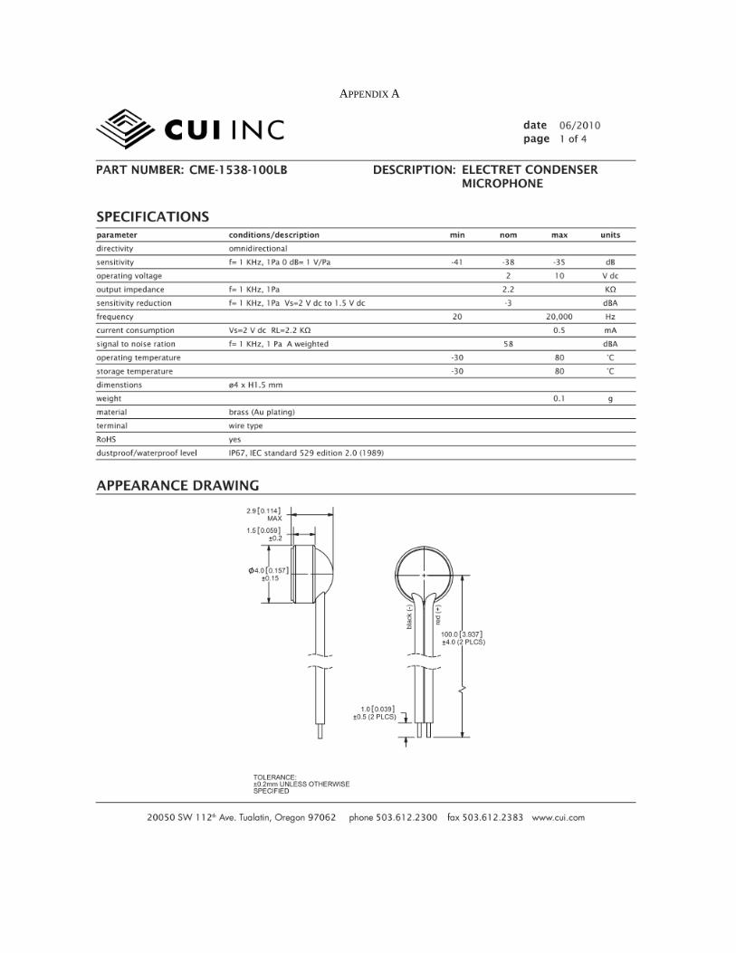
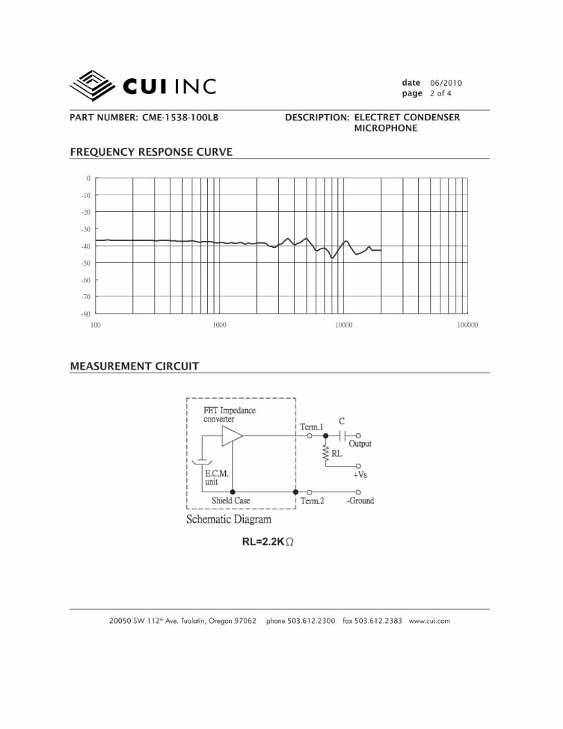
To collect acoustic emission, microphones are needed. We decided to use CUI INC microphone, part number CME-1538-100LB. It has a dimension of ø4 x H1.5 mm, which is small enough for our detection purpose. It also has a sensitivity of [-41, -35] dB, which is not ideal but the best we can find in a cost-effective price range. The current consumption under 2 volts dc is less than 0.5 mA, which is acceptable in our project. More information from the microphone can be gathered in the Appendix. After collecting acoustic signals, a little amount of analog filtering and amplification is needed, and operational amplifiers are chosen to perform this function. MCP 6004 chip was used in this project, it has a supply voltage range from 1.8 V to 6.0 V, which is appropriate for this project. Then after the signal is produced, it was fed into Arduino board where Fast Hartley transform (FHT) is performed. A FHT

5

is a similar method as Fast Fourier Transform (FFT) but it is specifically designed for real data and uses half as much processing power as the FFT, and it is implemented to obtain the frequency components of the signal. Finally the signal will be displayed on an android device through Bluetooth transmission.

One of the challenges is that the Arduino Uno can only provide positive voltages, therefore providing a negative voltage for the operational amplifier is impossible. To resolve this problem, a voltage divider is used to provide a middle level of voltage.

Table 3.1 Technical Specification

Aspect Value/Range

Input Voltage 5 Vdc

Microphones Operating Voltage 2 - 10 Vdc

Pass Band Frequency of Band Pass Filter 20 - 20,000 Hz

Output Serially transmitted data points for plotting

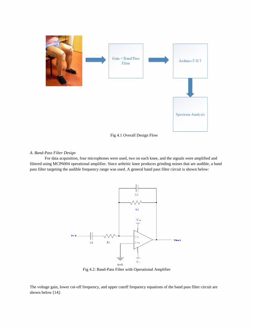
IV. DESIGN PROCEDURE Our method to diagnose the subject’s knee is to use a microphone in order to measure the different sounds coming from the knee. Two such microphones will be attached to each knee, along with other analog components. The analog signal coming from the microphones will go through a band-pass filter followed by a gain. The filter and the gain is made possible by an operational amplifier. After the signal is sent through the op-amp, an Arduino Uno will detect four signals in total, since there are four microphones. Based on the FHT library available online, our code will perform signal analysis and will ultimately provide the existing frequencies as well as their magnitude. Using MATLAB and possibly an Android device, we will be able to graph the various frequencies where we can more easily detect the peak frequency. Afterwards we can determine whether the location of that peak frequency as well as its magnitude represents a possible injured knee. Below is a schematic representation of our overall project design.

6

Fig 4.1 Overall Design Flow

A. Band-Pass Filter Design For data acquisition, four microphones were used, two on each knee, and the signals were amplified and filtered using MCP6004 operational amplifier. Since arthritic knee produces grinding noises that are audible, a band pass filter targeting the audible frequency range was used. A general band pass filter circuit is shown below:

Fig 4.2: Band-Pass Filter with Operational Amplifier

The voltage gain, lower cut-off frequency, and upper cutoff frequency equations of the band pass filter circuit are shown below [14]:

7

Gain = −R2

R1

Equation 1

fc1 = 1

2πR1C1

Equation 2

fc1 = 1

2πR2C2

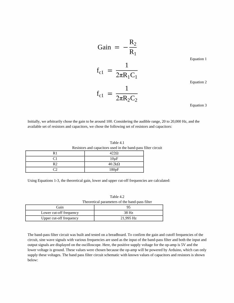
Equation 3 Initially, we arbitrarily chose the gain to be around 100. Considering the audible range, 20 to 20,000 Hz, and the available set of resistors and capacitors, we chose the following set of resistors and capacitors:

Table 4.1 Resistors and capacitors used in the band-pass filter circuit

R1 422Ω C1 10µF R2 40.2kΩ C2 180pF

Using Equations 1-3, the theoretical gain, lower and upper cut-off frequencies are calculated:

Table 4.2 Theoretical parameters of the band-pass filter

Gain 95 Lower cut-off frequency 38 Hz Upper cut-off frequency 21,995 Hz

The band-pass filter circuit was built and tested on a breadboard. To confirm the gain and cutoff frequencies of the circuit, sine wave signals with various frequencies are used as the input of the band-pass filter and both the input and output signals are displayed on the oscilloscope. Here, the positive supply voltage for the op-amp is 5V and the lower voltage is ground. These values were chosen because the op-amp will be powered by Arduino, which can only supply these voltages. The band pass filter circuit schematic with known values of capacitors and resistors is shown below:

8

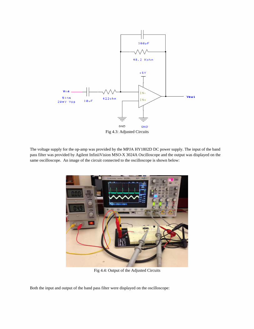
Fig 4.3: Adjusted Circuits

The voltage supply for the op-amp was provided by the MPJA HY1802D DC power supply. The input of the band pass filter was provided by Agilent InfiniiVision MSO-X 3024A Oscilloscope and the output was displayed on the same oscilloscope. An image of the circuit connected to the oscilloscope is shown below:

Fig 4.4: Output of the Adjusted Circuits

Both the input and output of the band pass filter were displayed on the oscilloscope:

9

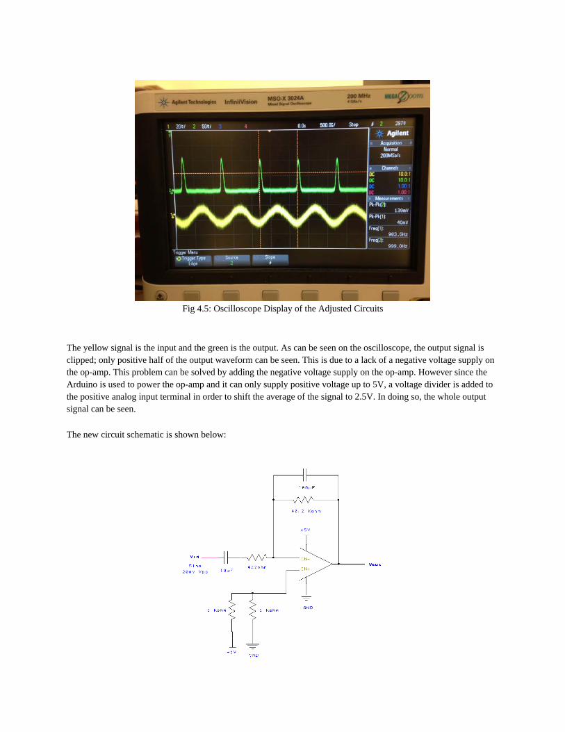
Fig 4.5: Oscilloscope Display of the Adjusted Circuits

The yellow signal is the input and the green is the output. As can be seen on the oscilloscope, the output signal is clipped; only positive half of the output waveform can be seen. This is due to a lack of a negative voltage supply on the op-amp. This problem can be solved by adding the negative voltage supply on the op-amp. However since the Arduino is used to power the op-amp and it can only supply positive voltage up to 5V, a voltage divider is added to the positive analog input terminal in order to shift the average of the signal to 2.5V. In doing so, the whole output signal can be seen. The new circuit schematic is shown below:

10

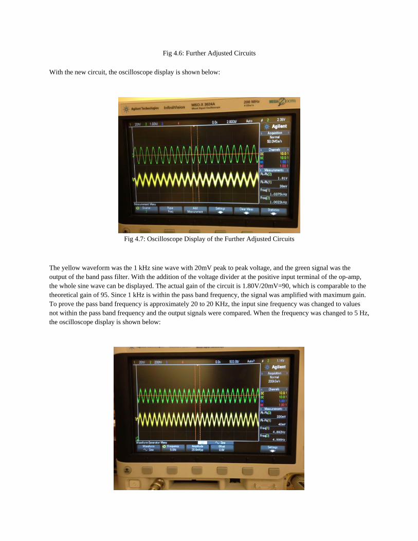
Fig 4.6: Further Adjusted Circuits With the new circuit, the oscilloscope display is shown below:

Fig 4.7: Oscilloscope Display of the Further Adjusted Circuits

The yellow waveform was the 1 kHz sine wave with 20mV peak to peak voltage, and the green signal was the output of the band pass filter. With the addition of the voltage divider at the positive input terminal of the op-amp, the whole sine wave can be displayed. The actual gain of the circuit is 1.80V/20mV=90, which is comparable to the theoretical gain of 95. Since 1 kHz is within the pass band frequency, the signal was amplified with maximum gain. To prove the pass band frequency is approximately 20 to 20 KHz, the input sine frequency was changed to values not within the pass band frequency and the output signals were compared. When the frequency was changed to 5 Hz, the oscilloscope display is shown below:

11

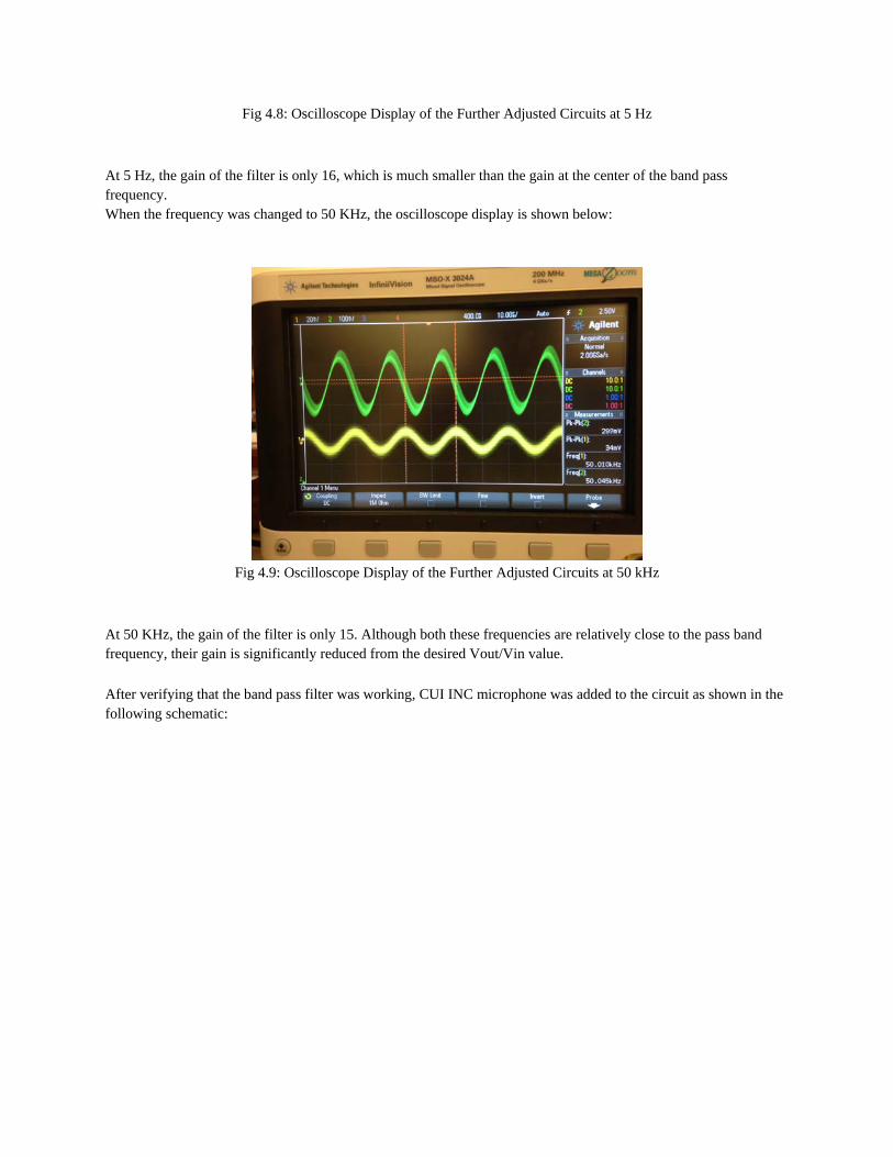
Fig 4.8: Oscilloscope Display of the Further Adjusted Circuits at 5 Hz

At 5 Hz, the gain of the filter is only 16, which is much smaller than the gain at the center of the band pass frequency. When the frequency was changed to 50 KHz, the oscilloscope display is shown below:

Fig 4.9: Oscilloscope Display of the Further Adjusted Circuits at 50 kHz

At 50 KHz, the gain of the filter is only 15. Although both these frequencies are relatively close to the pass band frequency, their gain is significantly reduced from the desired Vout/Vin value. After verifying that the band pass filter was working, CUI INC microphone was added to the circuit as shown in the following schematic:

12

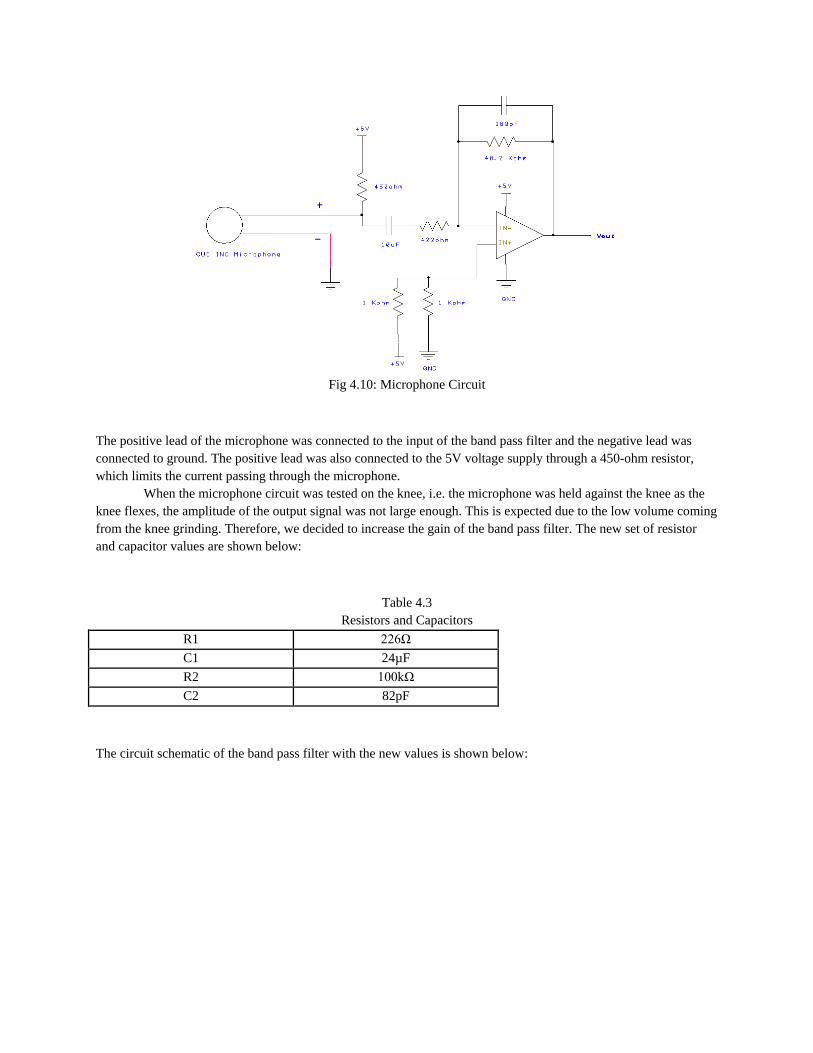
Fig 4.10: Microphone Circuit

The positive lead of the microphone was connected to the input of the band pass filter and the negative lead was connected to ground. The positive lead was also connected to the 5V voltage supply through a 450-ohm resistor, which limits the current passing through the microphone. When the microphone circuit was tested on the knee, i.e. the microphone was held against the knee as the knee flexes, the amplitude of the output signal was not large enough. This is expected due to the low volume coming from the knee grinding. Therefore, we decided to increase the gain of the band pass filter. The new set of resistor and capacitor values are shown below:

Table 4.3 Resistors and Capacitors

R1 226Ω C1 24µF R2 100kΩ C2 82pF

The circuit schematic of the band pass filter with the new values is shown below:

13

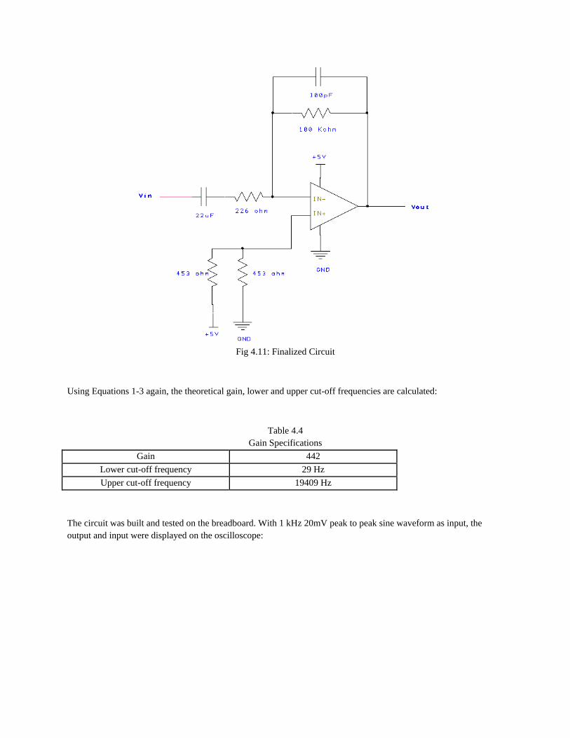
Fig 4.11: Finalized Circuit

Using Equations 1-3 again, the theoretical gain, lower and upper cut-off frequencies are calculated:

Table 4.4 Gain Specifications

Gain 442 Lower cut-off frequency 29 Hz Upper cut-off frequency 19409 Hz

The circuit was built and tested on the breadboard. With 1 kHz 20mV peak to peak sine waveform as input, the output and input were displayed on the oscilloscope:

14

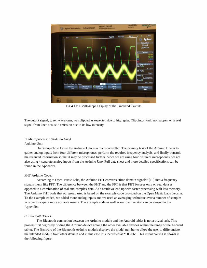
Fig 4.11: Oscilloscope Display of the Finalized Circuits

The output signal, green waveform, was clipped as expected due to high gain. Clipping should not happen with real signal from knee acoustic emission due to its low intensity. B. Microprocessor (Arduino Uno) Arduino Uno: Our group chose to use the Arduino Uno as a microcontroller. The primary task of the Arduino Uno is to gather analog inputs from four different microphones, perform the required frequency analysis, and finally transmit the received information so that it may be processed further. Since we are using four different microphones, we are also using 4 separate analog inputs from the Arduino Uno. Full data sheet and more detailed specifications can be found in the Appendix. FHT Arduino Code: According to Open Music Labs, the Arduino FHT converts “time domain signals” [15] into a frequency signals much like FFT. The difference between the FHT and the FFT is that FHT focuses only on real data as opposed to a combination of real and complex data. As a result we end up with faster processing with less memory. The Arduino FHT code that our group used is based on the example code provided on the Open Music Labs website. To the example coded, we added more analog inputs and we used an averaging technique over a number of samples in order to acquire more accurate results. The example code as well as our own version can be viewed in the Appendix. C. Bluetooth TX/RX

The Bluetooth connection between the Arduino module and the Android tablet is not a trivial task. This process first begins by finding the Arduino device among the other available devices within the range of the Android tablet. The firmware of the Bluetooth Arduino module displays the model number to allow the user to differentiate the intended module from other devices and in this case it is identified as “HC-06”. This initial pairing is shown in the following figure.

15

Fig 4.12: Android Bluetooth Setting Page

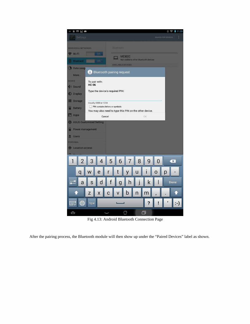
Upon initiating the pairing request, the user is required to input a PIN number. The factory values were used in this instance for simplicity but in the situation of a production model, these would be changed to negate cross communication with other unintended devices. The process of pairing is shown here.

16

Fig 4.13: Android Bluetooth Connection Page

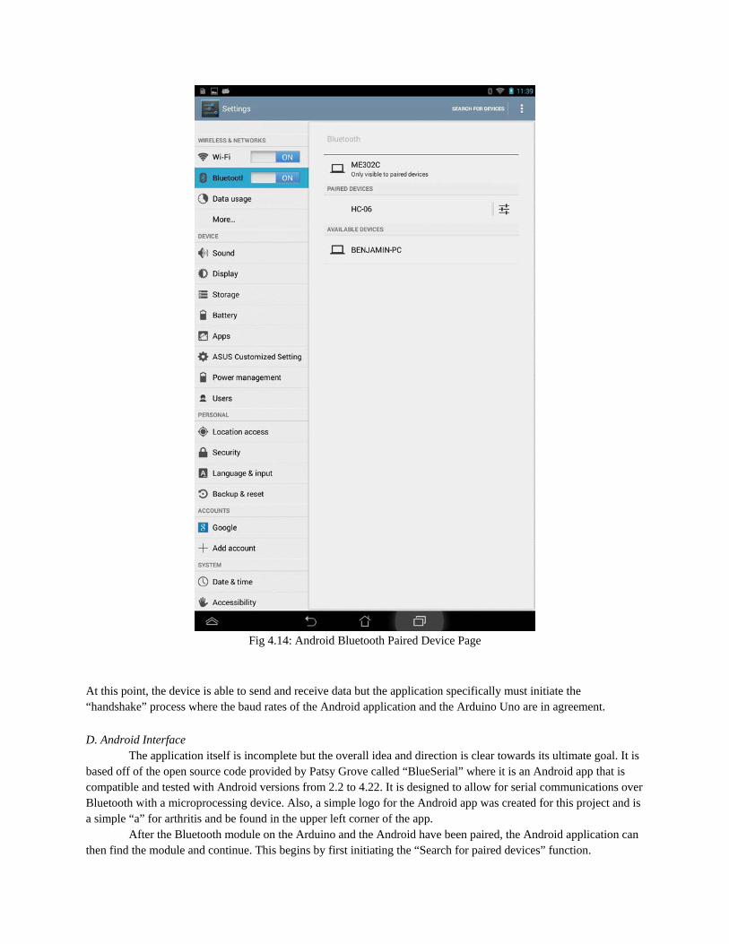
After the pairing process, the Bluetooth module will then show up under the “Paired Devices” label as shown.

17

Fig 4.14: Android Bluetooth Paired Device Page

At this point, the device is able to send and receive data but the application specifically must initiate the “handshake” process where the baud rates of the Android application and the Arduino Uno are in agreement. D. Android Interface

The application itself is incomplete but the overall idea and direction is clear towards its ultimate goal. It is based off of the open source code provided by Patsy Grove called “BlueSerial” where it is an Android app that is compatible and tested with Android versions from 2.2 to 4.22. It is designed to allow for serial communications over Bluetooth with a microprocessing device. Also, a simple logo for the Android app was created for this project and is a simple “a” for arthritis and be found in the upper left corner of the app.

After the Bluetooth module on the Arduino and the Android have been paired, the Android application can then find the module and continue. This begins by first initiating the “Search for paired devices” function.

18

Fig 4.15: Android App Startup

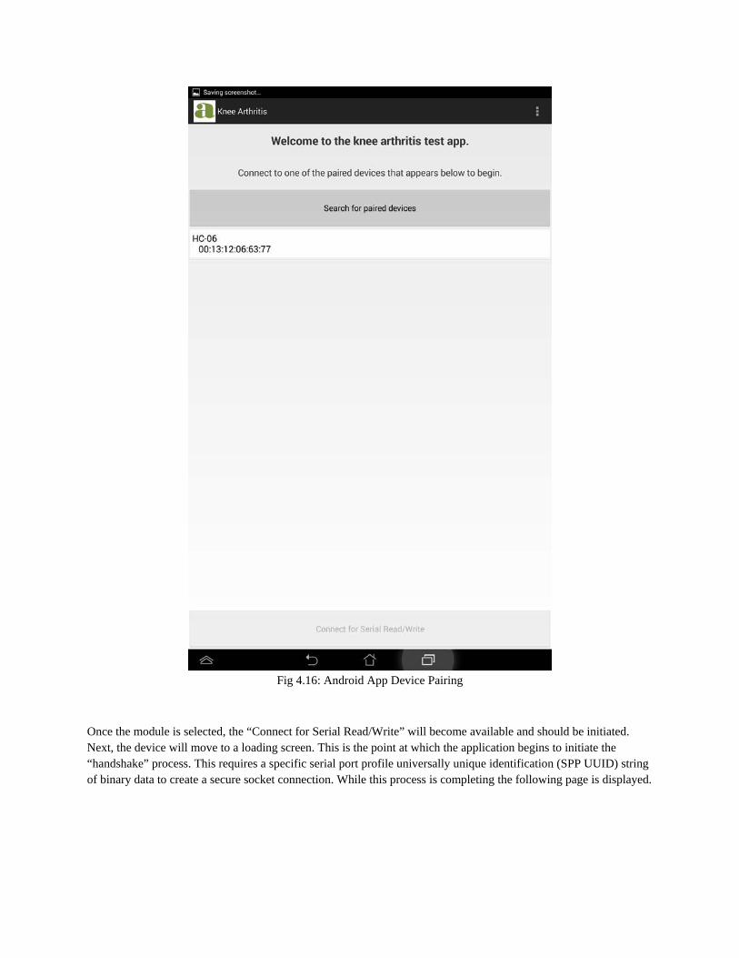
After the device is allowed to search, the Bluetooth device will become available, along with any other devices that have been previously paired with the device. In this instance, only the “HC-06” module is displayed along with its corresponding MAC address.

19

Fig 4.16: Android App Device Pairing

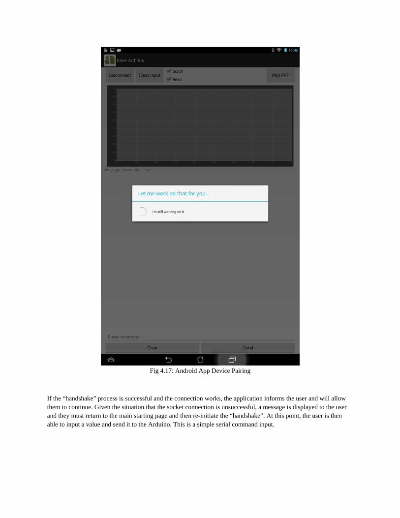
Once the module is selected, the “Connect for Serial Read/Write” will become available and should be initiated. Next, the device will move to a loading screen. This is the point at which the application begins to initiate the “handshake” process. This requires a specific serial port profile universally unique identification (SPP UUID) string of binary data to create a secure socket connection. While this process is completing the following page is displayed.

20

Fig 4.17: Android App Device Pairing

If the “handshake” process is successful and the connection works, the application informs the user and will allow them to continue. Given the situation that the socket connection is unsuccessful, a message is displayed to the user and they must return to the main starting page and then re-initiate the “handshake”. At this point, the user is then able to input a value and send it to the Arduino. This is a simple serial command input.

21

Fig 4.18: Android App Device Paired

Once the serial command has been sent to the Arduino, the data collection process will begin and the Android tablet is simply listening for the output. Since there is no stated values that are directly expected to be collected, the session fundamentally cannot be timed out. This is a useful feature because it allows for easy data collection but it can become troublesome in that data can inadvertently be overwritten or be stored incorrectly. The sent data on the serial ports from the Arduino will be displayed as text below the region designed for a dynamic plot of the data. The plotting aspect was unsuccessfully completed on this page but space was made available and can be seen in the following figure.

22

Fig 4.20: Android App Data Received

Once the data was collected and displayed further functionality could be implemented. A button was created to be able to save the data for later inspection or for tracking purposes and to give the user more information about their arthritis condition. As it stands, this aspect was left incomplete but a button was created to allow for a single line of analog input from the Arduino to be displayed as shown in the next figure.

23

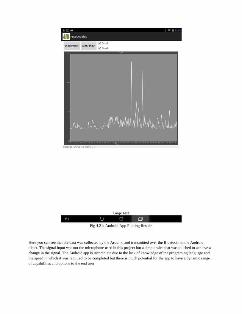
Fig 4.21: Android App Plotting Results

Here you can see that the data was collected by the Arduino and transmitted over the Bluetooth to the Android tablet. The signal input was not the microphone used in this project but a simple wire that was touched to achieve a change in the signal. The Android app is incomplete due to the lack of knowledge of the programing language and the speed in which it was required to be completed but there is much potential for the app to have a dynamic range of capabilities and options to the end user.

24

V. SIMULATION RESULTS

This part includes all the schematics and results from the simulation. The simulation software used in this project is the Cadence Allegro design entry CIS. The main reason we chose this software is that there is a tutorial taught in this class and it will be much easier to seek help in case of countering difficulties during simulations. The simulation schematic for the band pass amplifier is shown in the following figure. The values of the analog components are chosen to match the actual values that can be found and used in the project.

Fig 5.1: Simulation Schematic for Band-Pass Amplifier

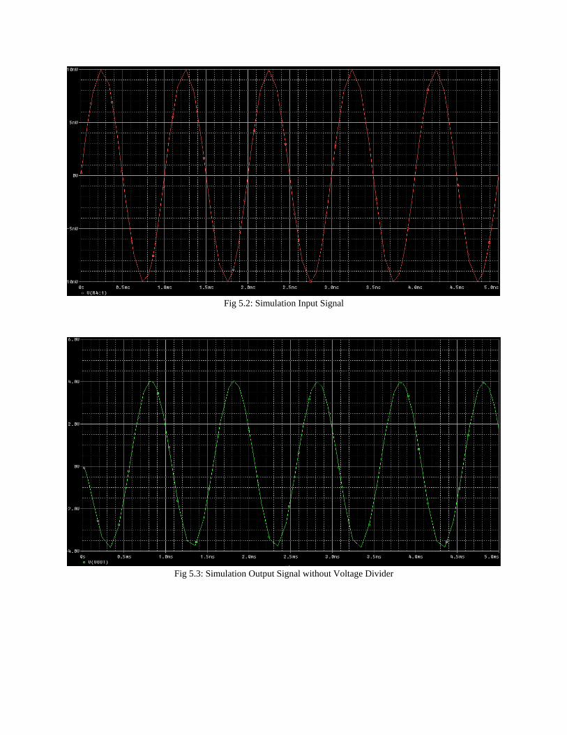
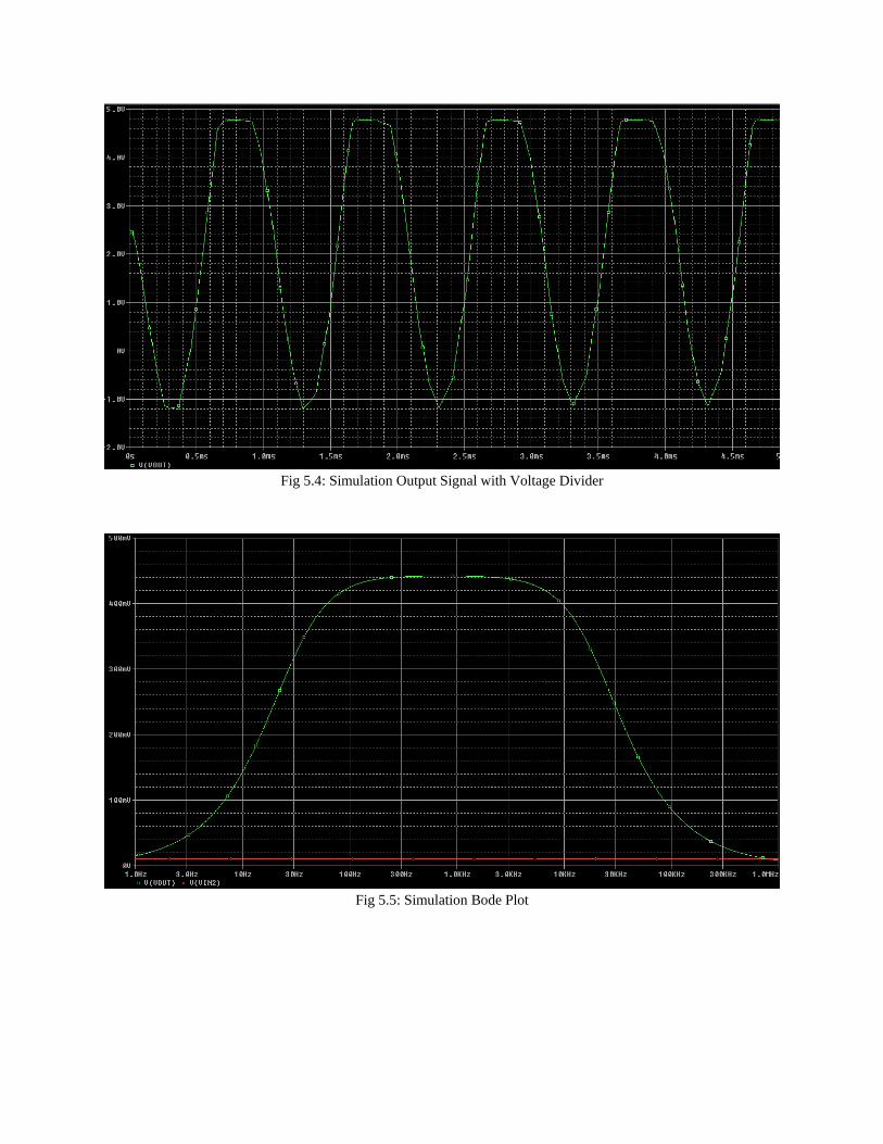
The following figures show the simulation results. The amplification gain (output/input) is about 400, which is within 10% of the designed gain. This difference is very likely caused by the operation amplifier that is used in the simulation. Additionally, based on the bode plot response shown in Fig 5.5, the 3dB pass band is roughly from 40 Hz to 20 kHz, which matches the designed pass band range in table 4.4 . Additionally, by introducing the voltage divider, the actual useable voltage range is actually cut in half, which is the reason saturation appeared in fig 5.4. However, in the actual project, the acoustic signal from the knee is very weak, therefore saturation would never be a problem.

25

Fig 5.2: Simulation Input Signal

Fig 5.3: Simulation Output Signal without Voltage Divider

26

Fig 5.4: Simulation Output Signal with Voltage Divider

Fig 5.5: Simulation Bode Plot

27

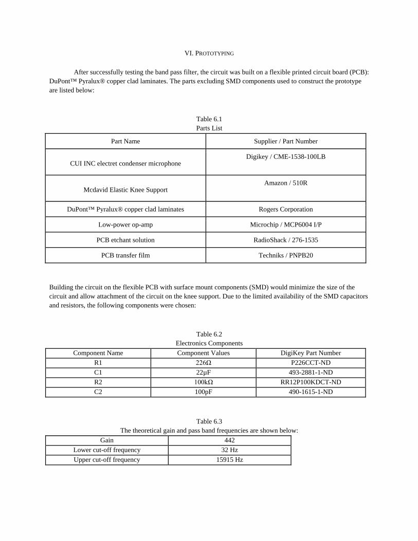
VI. PROTOTYPING After successfully testing the band pass filter, the circuit was built on a flexible printed circuit board (PCB): DuPont™ Pyralux® copper clad laminates. The parts excluding SMD components used to construct the prototype are listed below:

Table 6.1 Parts List

Part Name Supplier / Part Number

CUI INC electret condenser microphone Digikey / CME-1538-100LB

Mcdavid Elastic Knee Support Amazon / 510R

DuPont™ Pyralux® copper clad laminates Rogers Corporation

Low-power op-amp Microchip / MCP6004 I/P

PCB etchant solution RadioShack / 276-1535

PCB transfer film Techniks / PNPB20

Building the circuit on the flexible PCB with surface mount components (SMD) would minimize the size of the circuit and allow attachment of the circuit on the knee support. Due to the limited availability of the SMD capacitors and resistors, the following components were chosen:

Table 6.2 Electronics Components

Component Name Component Values DigiKey Part Number R1 226Ω P226CCT-ND C1 22µF 493-2881-1-ND R2 100kΩ RR12P100KDCT-ND C2 100pF 490-1615-1-ND

Table 6.3 The theoretical gain and pass band frequencies are shown below:

Gain 442 Lower cut-off frequency 32 Hz Upper cut-off frequency 15915 Hz

28

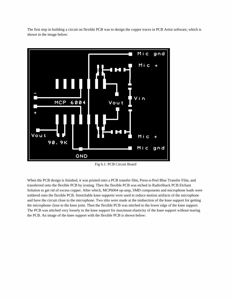
The first step in building a circuit on flexible PCB was to design the copper traces in PCB Artist software, which is shown in the image below:

Fig 6.1: PCB Circuit Board

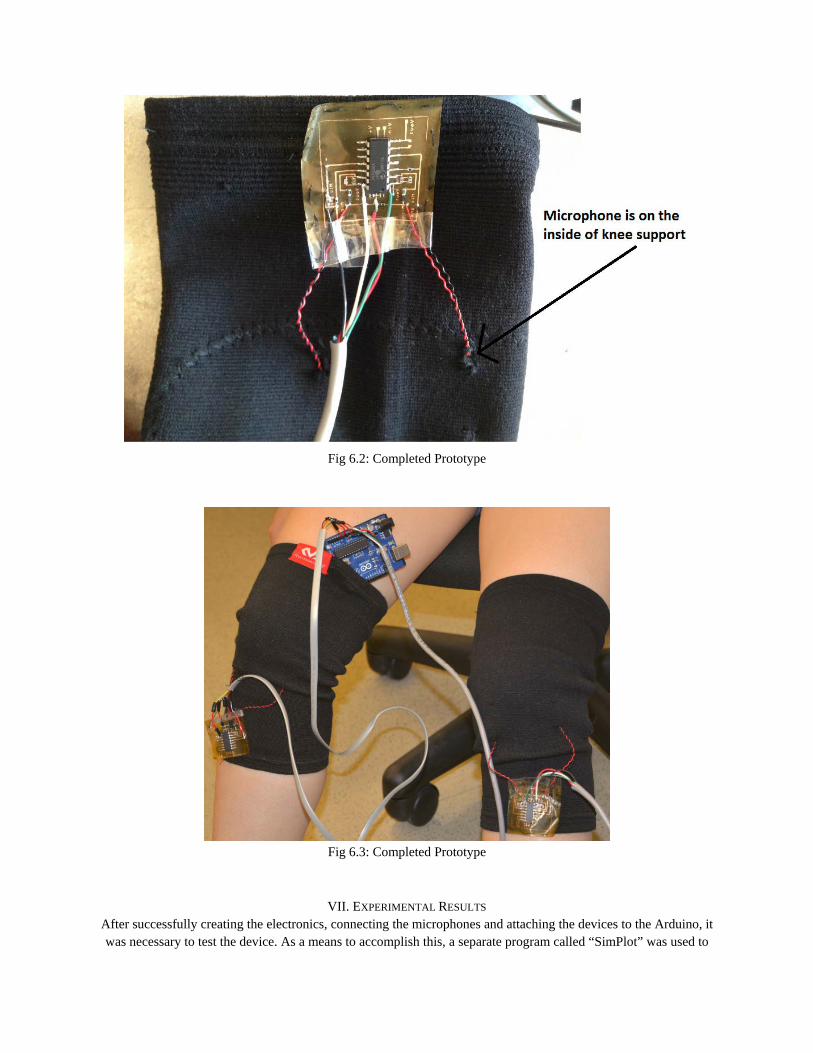
When the PCB design is finished, it was printed onto a PCB transfer film, Press-n-Peel Blue Transfer Film, and transferred onto the flexible PCB by ironing. Then the flexible PCB was etched in RadioShack PCB Etchant Solution to get rid of excess copper. After which, MCP6004 op-amp, SMD components and microphone leads were soldered onto the flexible PCB. Stretchable knee supports were used to reduce motion artifacts of the microphone and have the circuit close to the microphone. Two slits were made at the midsection of the knee support for getting the microphone close to the knee joint. Then the flexible PCB was stitched to the lower edge of the knee support. The PCB was stitched very loosely to the knee support for maximum elasticity of the knee support without tearing the PCB. An image of the knee support with the flexible PCB is shown below:

29

Fig 6.2: Completed Prototype

Fig 6.3: Completed Prototype

VII. EXPERIMENTAL RESULTS After successfully creating the electronics, connecting the microphones and attaching the devices to the Arduino, it was necessary to test the device. As a means to accomplish this, a separate program called “SimPlot” was used to

30

quickly test and analyze the output signal from the Arduino. It is another open source code that is implemented on a Windows platform and uses the serial port connections between the PC and the Android. Simplot is simple to use

but dynamic in its ability to display the output of the Arduino with clarity. The two images below are screen captures of the live sound stream coming from the left and right knee respectively where different colors represent

the different channel inputs to the Arduino.

Fig 7.1: Live Stream received from left knee microphones

Fig 7.2: Live stream received from right knee microphones

Here we can see that all four signals are resting at approximately the midpoint of the range available for the Arduino to display at 512. The reason that the Arduino can only transmit signal values from 0 to 1024 is due to the limiting

31

facilities of the processors capability to read analog signals through its analog to digital converter. These converters read a voltage value and transform it into a value encoded digitally. In each of the above cases, the two microphones on each knee brace has been tapped to ensure that sound is being captured and detected successfully. In the following figure all four microphones are taped over the displayed time separately and do not interfere with each other.

Fig 7.3: Livestream of all the microphones in both knees

This process demonstrates that the sound can be collected and distinguished for each individual microphone given that it is large enough and well above the ambient electronic noise of the Arduino device and additional circuit boards. Bluetooth Transmitter: Once the signal was shown to give a reasonable output, the Bluetooth module was added to the Arduino to give it the originally designed full functionality. This then started to show a series of signal degradations that was not fully understood. As a means to at least follow the trends of the signal, the Simplot program was used again. When the Bluetooth module was added but not paired with the Android tablet, it blinks and as it blinks the signal collected fluctuated. This unforeseen noise can be found in the next figure and it was assumed that the blinking was changing the voltage on the Arduino board and therefore negatively impacting the analog serial input signals.

32

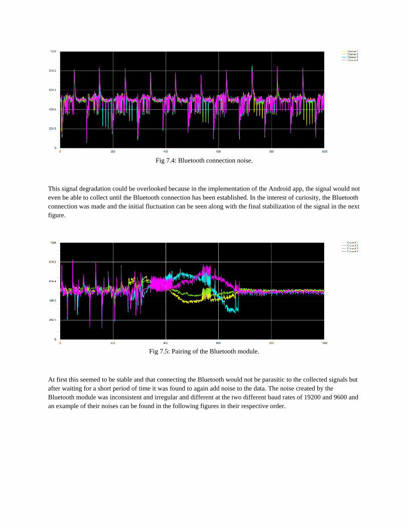
Fig 7.4: Bluetooth connection noise.

This signal degradation could be overlooked because in the implementation of the Android app, the signal would not even be able to collect until the Bluetooth connection has been established. In the interest of curiosity, the Bluetooth connection was made and the initial fluctuation can be seen along with the final stabilization of the signal in the next figure.

Fig 7.5: Pairing of the Bluetooth module.

At first this seemed to be stable and that connecting the Bluetooth would not be parasitic to the collected signals but after waiting for a short period of time it was found to again add noise to the data. The noise created by the Bluetooth module was inconsistent and irregular and different at the two different baud rates of 19200 and 9600 and an example of their noises can be found in the following figures in their respective order.

33

Fig 7.6: Bluetooth resonant noise at the 19200 baud rate.

Fig 7.7: Bluetooth resonant noise at the 9600 baud rate.

Ultimately, the Bluetooth module was abandoned because of its many problems that were unable to be resolved. Signal after FHT: Due to complications with creating the Android application to its fullest capacity within the allotted time and difficulties in resolving the noise generated by the Bluetooth module, a MATLAB code was created to read and interpret the output of the Arduino’s FHT signal and automatically generate a plot for ease of user interpretation. This code can be found in the appendix.

The MATLAB code was designed to be able to display each individual microphone separately or to average the two microphones for each individual knee. Being able to view and capture each signal could allow for a more complete analysis while being able to view each knee on a macroscopic scale may be easier for the end user to understand. It was also deemed important to follow the behavior of the device fully assembled, so one of the knee brace assemblies was attached to the Arduino and the other input signals were left open. The resulting FHT signal generated by the Arduino can be seen in the next figure where the blue line represents the averaged signal from the knee brace assembly without a patient and the green represents the average of the open inputs.

34

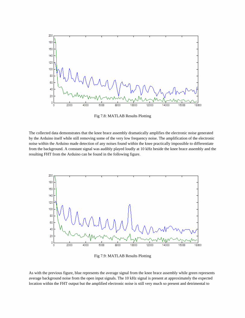
Fig 7.8: MATLAB Results Plotting

The collected data demonstrates that the knee brace assembly dramatically amplifies the electronic noise generated by the Arduino itself while still removing some of the very low frequency noise. The amplification of the electronic noise within the Arduino made detection of any noises found within the knee practically impossible to differentiate from the background. A constant signal was audibly played loudly at 10 kHz beside the knee brace assembly and the resulting FHT from the Arduino can be found in the following figure.

Fig 7.9: MATLAB Results Plotting

As with the previous figure, blue represents the average signal from the knee brace assembly while green represents average background noise from the open input signals. The 10 kHz signal is present at approximately the expected location within the FHT output but the amplified electronic noise is still very much so present and detrimental to

35

drawing any conclusive decisions about the signal without any previous knowledge. Given that the sounds produced by the grinding of the knee would be quite faint and over a range of frequencies, it would be exceptionally difficult to locate any particular problem with the amplified electronic noise present.

VIII. CONCLUSION

Signal Acquisition: The Arduino Uno performed well for the analog sound acquisition. As the live stream images depict above, we were able to detect the sound signals pretty well. This worked well with louder sounds such as music being played, tapping the microphone, and general conversations. Overall we were limited by the microphone sound quality and not the Arduino. Live streaming of the signal: Prior to performing the frequency analysis it was important to be able to detect anything at all. A simple live stream code included in the Appendix helped confirm sound acquisition from the Arduino. Amplified Signal without Bluetooth Transmitter: The filtered and amplified signal transmitted to the Arduino remained uninfluenced when the Bluetooth connection was left off. Transmitting the signal information to MATLAB through the USB port had no influence on the incoming signal. This proved to be a reliable way to display the frequency analysis performed by the Arduino. Amplified Signal with Bluetooth Transmitter: Although we successfully coupled the Arduino with an android device via Bluetooth, it significantly influenced our incoming signal. It is unclear how exactly this occurred, but a major source of noise was detected once the Bluetooth was connected. This completely changed our live stream image, rendering it unrecognizable based on prior signal acquisitions. Signal after FHT: By modifying the FHT code provided in the Arduino FHT library, we were able to apply a solid frequency analyzer to our incoming sound. Although the Arduino has a limited sampling rate when compared to larger computers, it functions well enough to successfully provide us with a general peak frequency. Taking into account that we have four separate signals transmitting to the Arduino, it handled the signal load pretty well. Obstacles during the Process One of the biggest obstacles we encountered during this project is the poor connection of the wires. A lot of times, problems are caused simply from dysfunctional wires and it took us hours to find out that there was nothing wrong with the actual circuit. Furthermore, the wires also provided a major source of resistance. With the incoming and outgoing signals remaining pretty small, any loss influenced the measurement. Another obstacle was the sound quality transmitted by the microphone. As mentioned before, music, conversations, as well as microphone taps, were all easily detectable by microphone and the Arduino. Fainter sound like knee grinding noises, are not as easily detectable by our chosen microphone. A third obstacle was the FHT code. Although it worked well for us, the code is not as accurate as an FFT. Since the advantage of the FHT is to reduce processing time, it may have lacked accuracy during the frequency analysis process. Further Improvements The easiest improvement we can make is to purchase a better microphone. With a higher frequency as well as amplitude range, we could more easily detect fainter sounds. Furthermore, higher end microphones might be able

36

to independently filter out unwanted noise in the environment. Since price is always an issue, this part of the project can always be improved. Another improvement we can make is to enhance the Arduino code in order to provide a more accurate frequency analysis. In the future this might mean using a different library altogether and perhaps combining several programs to obtain better spectrum acquisition. More knee sound information would also improve our project outcome. With a better microphone we could obtain better sound analysis on a healthy knee in order to exclude such cases. Lastly, in order to better display our findings we could develop an Android app that might could potentially connect via Bluetooth, assuming no noise is introduced by it.

37

REFERENCES

[1] Arthritis-Related Statistics., Centers for Disease Control and Prevention, [online], 2011 http://www.cdc.gov/arthritis/data_statistics/arthritis_related_stats.htm, (Accessed: February 24, 2014) [2] L.-K. Shark, H. Chen, J. Goodacre, Knee acoustic emission: A potential biomarker for quantitative assessment of joint ageing and degeneration, Medical Engineering & Physics, Volume 33, Issue 5, June 2011, Pages 534-545, ISSN 1350-4533, [3] B. Mascaro, J. Prior, L.-K. Shark, J. Selfe, P. Cole, J. Goodacre, Exploratory study of a non-invasive method based on acoustic emission for assessing the dynamic integrity of knee joints, Medical Engineering & Physics, Volume 31, Issue 8 [4] Arthritis., NYTimes.com, [online] 2013, http://www.nytimes.com/health/guides/disease/arthritis, (Accessed: February 24, 2014) [5] Osteoarthritis Health Center., WebMD, [online] 2005, http://www.webmd.com/osteoarthritis/, (Accessed: February 24, 2014) [6] Information About Arthritis., Orthopedics.about.com,[online], http://orthopedics.about.com/od/arthritis/, (Accessed: February 24,2014) [7] Arthritis., Wikipedia.org, [online], http://en.wikipedia.org/wiki/Arthritis, (Accessed: February 24, 2014) [8] Mayo Clinic Health Letter., MayoClinic.com, [online], http://healthletter.mayoclinic.com/content/preview.cfm/n/288/t/Rheumatoid%20arthritis/, (Accessed: February, 24, 2014) [9] About.com: Arthritis & Joint Conditions, [online], http://arthritis.about.com/od/diagnostic/a/diagnosis.htm, (Accessed: February 24, 2014) [10] Rheumatoid Arthritis Health Center.,WebMD [online] 2005, http://www.webmd.com/rheumatoid-arthritis/guide/blood-tests, (Accessed: February 24, 2014) [11] T. C. Carlson, “Device for non-invasive diagnosis and monitoring of articular and periarticular pathology,” U.S. Patent US 07/155,033, Apr 25, 1989 [12] D. W. Lee, X. Banquy, J. N. Israelachvili. Stick-slip friction and wear of articular joints, Proceedings of the National Academy of Science, 2012. [13] Arduino., Wikipedia.org, [online], http://en.wikipedia.org/wiki/Arduino, (Accessed: February 24, 2014). [14] Active Band Pass Filter. Basic Electronics Tutorials, [online], http://www.electronics-tutorials.ws/filter/filter_7.html, (Accessed: May 2,

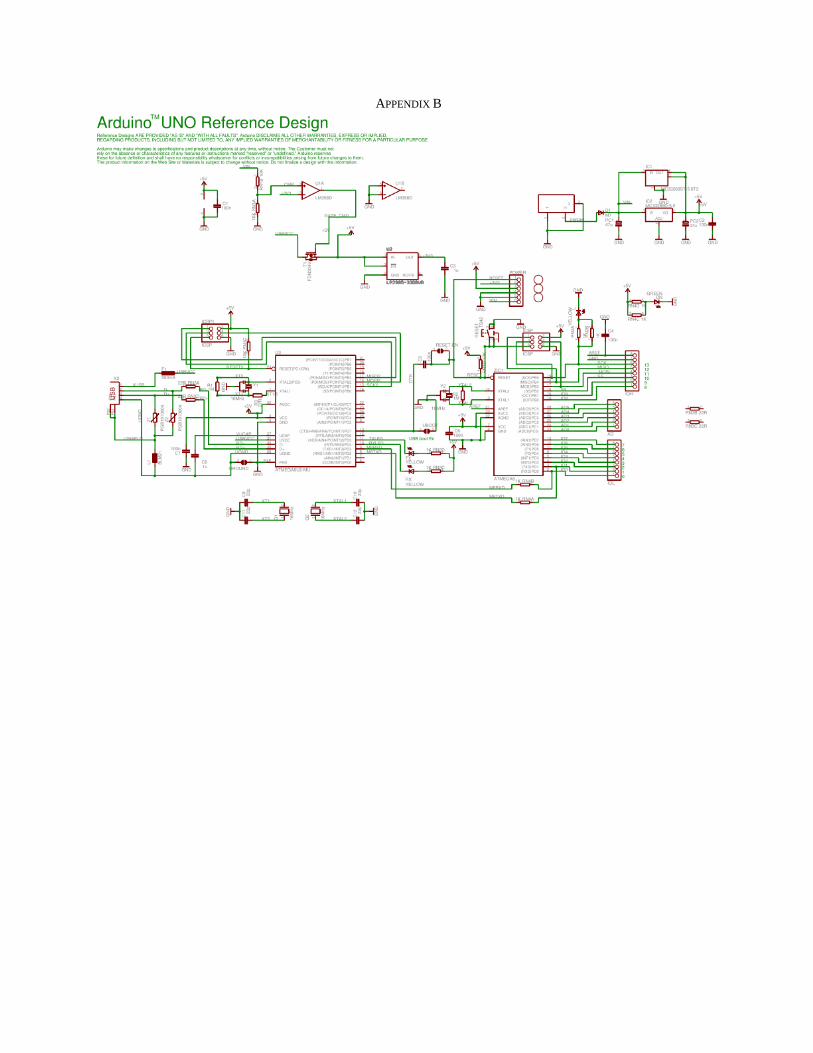
2014). [15] Open Music Labs. Arduino FHT Library [Online]. Available: http://wiki.openmusiclabs.com/wiki/ArduinoFHT [16] CUI INC, “Electret Condenser Microphone,” CME-1538-100LB data sheet, 06/2010. [17] Arduino, “Arduino UNO Reference Design,” [18] Microchip, “1MHZ, Low-Power Op Amp,” MCP6001/1R/1U/2/4 datasheet, 2008

38

APPENDIX A

39

40

APPENDIX B

41

APPENDIX C

42

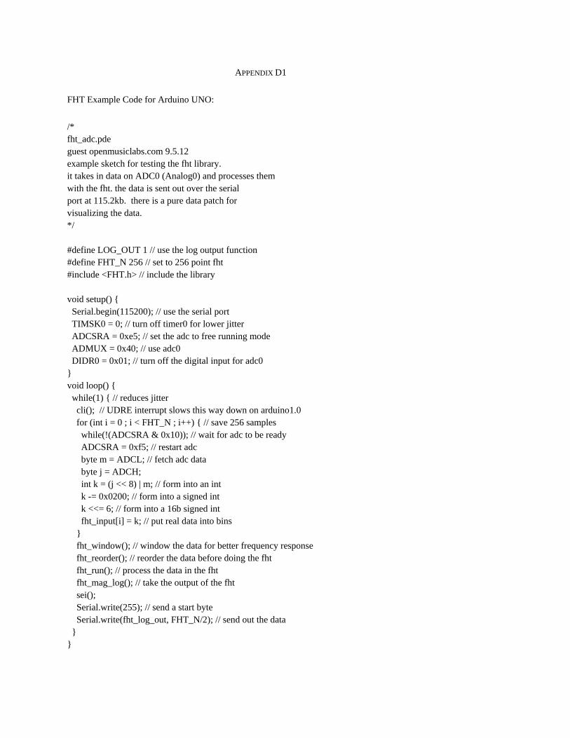
APPENDIX D1 FHT Example Code for Arduino UNO: /* fht_adc.pde guest openmusiclabs.com 9.5.12 example sketch for testing the fht library. it takes in data on ADC0 (Analog0) and processes them with the fht. the data is sent out over the serial port at 115.2kb. there is a pure data patch for visualizing the data. */ #define LOG_OUT 1 // use the log output function #define FHT_N 256 // set to 256 point fht #include <FHT.h> // include the library void setup() { Serial.begin(115200); // use the serial port TIMSK0 = 0; // turn off timer0 for lower jitter ADCSRA = 0xe5; // set the adc to free running mode ADMUX = 0x40; // use adc0 DIDR0 = 0x01; // turn off the digital input for adc0 } void loop() { while(1) { // reduces jitter cli(); // UDRE interrupt slows this way down on arduino1.0 for (int i = 0 ; i < FHT_N ; i++) { // save 256 samples while(!(ADCSRA & 0x10)); // wait for adc to be ready ADCSRA = 0xf5; // restart adc byte m = ADCL; // fetch adc data byte j = ADCH; int k = (j << 8) | m; // form into an int k -= 0x0200; // form into a signed int k <<= 6; // form into a 16b signed int fht_input[i] = k; // put real data into bins } fht_window(); // window the data for better frequency response fht_reorder(); // reorder the data before doing the fht fht_run(); // process the data in the fht fht_mag_log(); // take the output of the fht sei(); Serial.write(255); // send a start byte Serial.write(fht_log_out, FHT_N/2); // send out the data } }

43

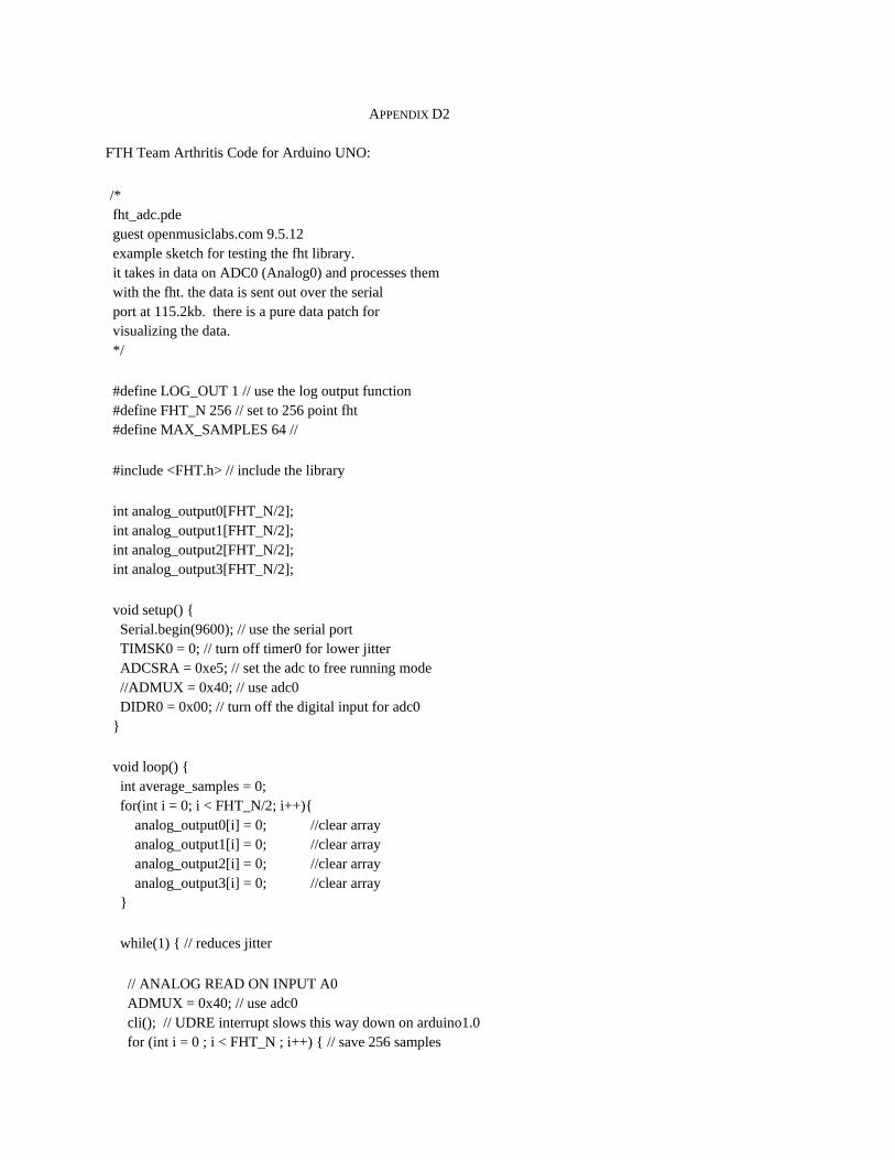
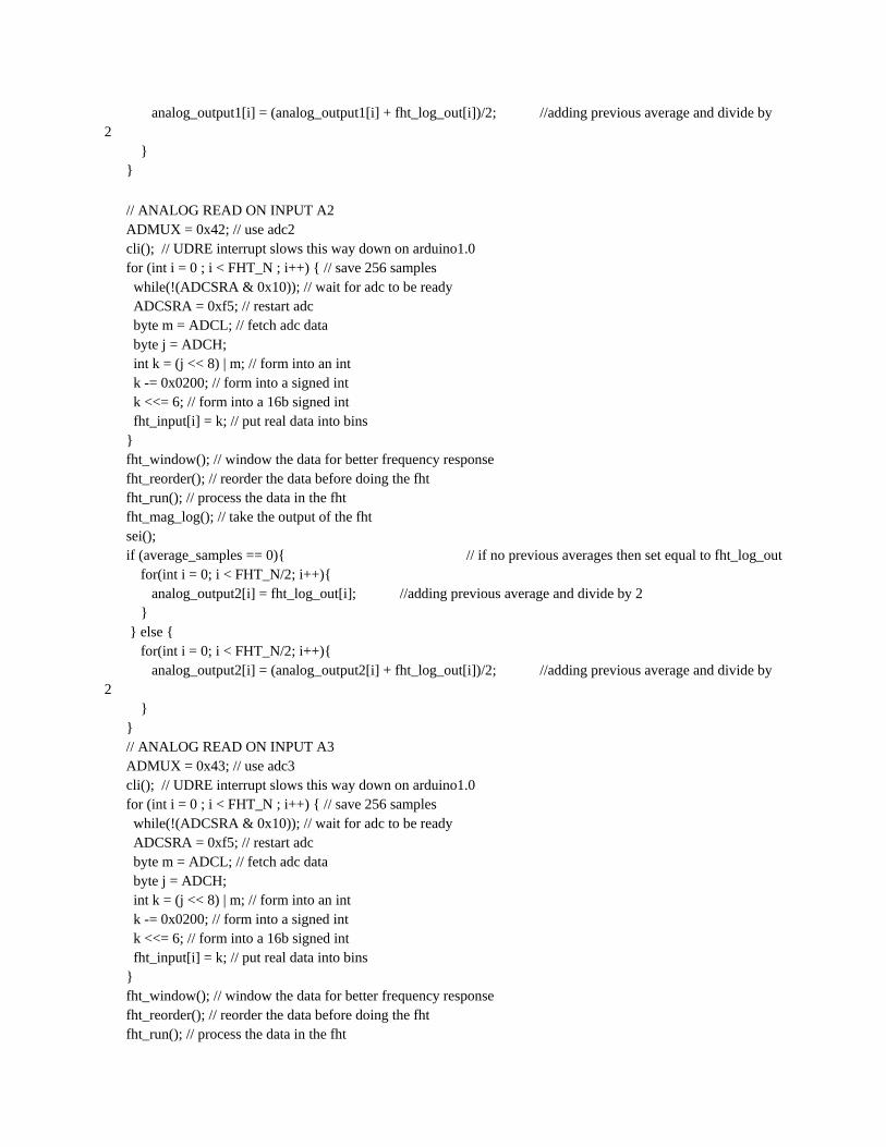
APPENDIX D2 FTH Team Arthritis Code for Arduino UNO: /* fht_adc.pde guest openmusiclabs.com 9.5.12 example sketch for testing the fht library. it takes in data on ADC0 (Analog0) and processes them with the fht. the data is sent out over the serial port at 115.2kb. there is a pure data patch for visualizing the data. */ #define LOG_OUT 1 // use the log output function #define FHT_N 256 // set to 256 point fht #define MAX_SAMPLES 64 // #include <FHT.h> // include the library int analog_output0[FHT_N/2]; int analog_output1[FHT_N/2]; int analog_output2[FHT_N/2]; int analog_output3[FHT_N/2]; void setup() { Serial.begin(9600); // use the serial port TIMSK0 = 0; // turn off timer0 for lower jitter ADCSRA = 0xe5; // set the adc to free running mode //ADMUX = 0x40; // use adc0 DIDR0 = 0x00; // turn off the digital input for adc0 } void loop() { int average_samples = 0; for(int i = 0; i < FHT_N/2; i++){ analog_output0[i] = 0; //clear array analog_output1[i] = 0; //clear array analog_output2[i] = 0; //clear array analog_output3[i] = 0; //clear array } while(1) { // reduces jitter // ANALOG READ ON INPUT A0 ADMUX = 0x40; // use adc0 cli(); // UDRE interrupt slows this way down on arduino1.0 for (int i = 0 ; i < FHT_N ; i++) { // save 256 samples

44

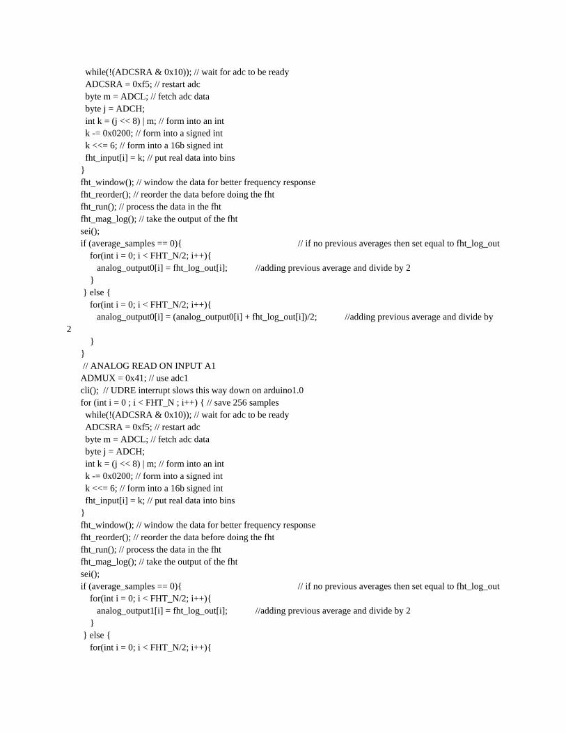
while(!(ADCSRA & 0x10)); // wait for adc to be ready ADCSRA = 0xf5; // restart adc byte m = ADCL; // fetch adc data byte j = ADCH; int k = (j << 8) | m; // form into an int k -= 0x0200; // form into a signed int k <<= 6; // form into a 16b signed int fht_input[i] = k; // put real data into bins } fht_window(); // window the data for better frequency response fht_reorder(); // reorder the data before doing the fht fht_run(); // process the data in the fht fht_mag_log(); // take the output of the fht sei(); if (average_samples == 0){ // if no previous averages then set equal to fht_log_out for(int i = 0; i < FHT_N/2; i++){ analog_output0[i] = fht_log_out[i]; //adding previous average and divide by 2 } } else { for(int i = 0; i < FHT_N/2; i++){ analog_output0[i] = (analog_output0[i] + fht_log_out[i])/2; //adding previous average and divide by 2 } } // ANALOG READ ON INPUT A1 ADMUX = 0x41; // use adc1 cli(); // UDRE interrupt slows this way down on arduino1.0 for (int i = 0 ; i < FHT_N ; i++) { // save 256 samples while(!(ADCSRA & 0x10)); // wait for adc to be ready ADCSRA = 0xf5; // restart adc byte m = ADCL; // fetch adc data byte j = ADCH; int k = (j << 8) | m; // form into an int k -= 0x0200; // form into a signed int k <<= 6; // form into a 16b signed int fht_input[i] = k; // put real data into bins } fht_window(); // window the data for better frequency response fht_reorder(); // reorder the data before doing the fht fht_run(); // process the data in the fht fht_mag_log(); // take the output of the fht sei(); if (average_samples == 0){ // if no previous averages then set equal to fht_log_out for(int i = 0; i < FHT_N/2; i++){ analog_output1[i] = fht_log_out[i]; //adding previous average and divide by 2 } } else { for(int i = 0; i < FHT_N/2; i++){

45

analog_output1[i] = (analog_output1[i] + fht_log_out[i])/2; //adding previous average and divide by 2 } } // ANALOG READ ON INPUT A2 ADMUX = 0x42; // use adc2 cli(); // UDRE interrupt slows this way down on arduino1.0 for (int i = 0 ; i < FHT_N ; i++) { // save 256 samples while(!(ADCSRA & 0x10)); // wait for adc to be ready ADCSRA = 0xf5; // restart adc byte m = ADCL; // fetch adc data byte j = ADCH; int k = (j << 8) | m; // form into an int k -= 0x0200; // form into a signed int k <<= 6; // form into a 16b signed int fht_input[i] = k; // put real data into bins } fht_window(); // window the data for better frequency response fht_reorder(); // reorder the data before doing the fht fht_run(); // process the data in the fht fht_mag_log(); // take the output of the fht sei(); if (average_samples == 0){ // if no previous averages then set equal to fht_log_out for(int i = 0; i < FHT_N/2; i++){ analog_output2[i] = fht_log_out[i]; //adding previous average and divide by 2 } } else { for(int i = 0; i < FHT_N/2; i++){ analog_output2[i] = (analog_output2[i] + fht_log_out[i])/2; //adding previous average and divide by 2 } } // ANALOG READ ON INPUT A3 ADMUX = 0x43; // use adc3 cli(); // UDRE interrupt slows this way down on arduino1.0 for (int i = 0 ; i < FHT_N ; i++) { // save 256 samples while(!(ADCSRA & 0x10)); // wait for adc to be ready ADCSRA = 0xf5; // restart adc byte m = ADCL; // fetch adc data byte j = ADCH; int k = (j << 8) | m; // form into an int k -= 0x0200; // form into a signed int k <<= 6; // form into a 16b signed int fht_input[i] = k; // put real data into bins } fht_window(); // window the data for better frequency response fht_reorder(); // reorder the data before doing the fht fht_run(); // process the data in the fht

46

fht_mag_log(); // take the output of the fht sei(); if (average_samples == 0){ // if no previous averages then set equal to fht_log_out for(int i = 0; i < FHT_N/2; i++){ analog_output3[i] = fht_log_out[i]; //adding previous average and divide by 2 } } else { for(int i = 0; i < FHT_N/2; i++){ analog_output3[i] = (analog_output3[i] + fht_log_out[i])/2; //adding previous average and divide by 2 } } average_samples++; if (average_samples >= MAX_SAMPLES){ for(int i = 0; i < FHT_N/2; i++){ Serial.print(i+1); Serial.print(" "); Serial.print(analog_output0[i]); Serial.print(" "); Serial.print(analog_output1[i]); Serial.print(" "); Serial.print(analog_output2[i]); Serial.print(" "); Serial.println(analog_output3[i]); analog_output0[i] = 0; //clear array analog_output1[i] = 0; //clear array analog_output2[i] = 0; //clear array analog_output3[i] = 0; //clear array } average_samples = 0; for(int i = 0; i < FHT_N/2; i++){ analog_output0[i] = 0; //clear array analog_output1[i] = 0; //clear array analog_output2[i] = 0; //clear array analog_output3[i] = 0; //clear array } while (Serial.available() == 0) ; // Wait here until input buffer has a character { int incomingByte = Serial.read(); //int Trial_Type = Serial.parseInt(); // new command in 1.0 forward //Serial.println("Trial 1 Selected "); } } } }

47

APPENDIX D3

Livestream Arduino UNO Code: int sensorPin0 = A0; int sensorPin1 = A1; int sensorPin2 = A2; int sensorPin3 = A3; void setup() { // Open serial communications and wait for port to open: Serial.begin(9600); } void loop() // run over and over { Serial.print(analogRead(sensorPin0)); Serial.print(" "); Serial.print(analogRead(sensorPin1)); Serial.print(" "); Serial.print(analogRead(sensorPin2)); Serial.print(" "); Serial.println(analogRead(sensorPin3)); }

48

APPENDIX E1

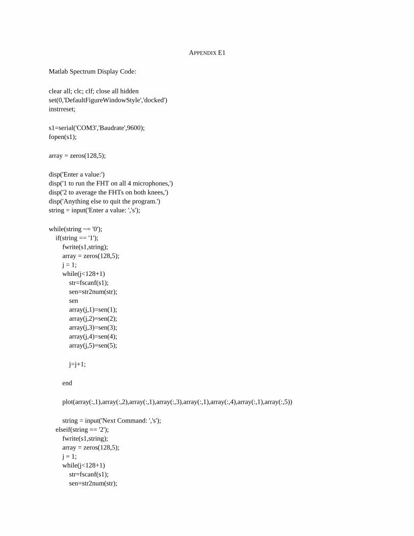
Matlab Spectrum Display Code: clear all; clc; clf; close all hidden set(0,'DefaultFigureWindowStyle','docked') instrreset; s1=serial('COM3','Baudrate',9600); fopen(s1); array = zeros(128,5); disp('Enter a value:') disp('1 to run the FHT on all 4 microphones,') disp('2 to average the FHTs on both knees,') disp('Anything else to quit the program.') string = input('Enter a value: ','s'); while(string ~= '0'); if(string == '1'); fwrite(s1,string); array = zeros(128,5); j = 1; while(j<128+1) str=fscanf(s1); sen=str2num(str); sen array(j,1)=sen(1); array(j,2)=sen(2); array(j,3)=sen(3); array(j,4)=sen(4); array(j,5)=sen(5); j=j+1; end plot(array(:,1),array(:,2),array(:,1),array(:,3),array(:,1),array(:,4),array(:,1),array(:,5)) string = input('Next Command: ','s'); elseif(string == '2'); fwrite(s1,string); array = zeros(128,5); j = 1; while(j<128+1) str=fscanf(s1); sen=str2num(str);

49

array(j,1)=sen(1); array(j,2)=sen(2); array(j,3)=sen(3); array(j,4)=sen(4); array(j,5)=sen(5); j=j+1; end plot(array(:,1),(array(:,2)+array(:,3))/2,array(:,1),(array(:,4)+array(:,5))/2) string = input('Next Command: ','s'); else disp('Not an option.') string = input('Enter a value: ','s'); end end fclose(s1); instrreset;

50

APPENDIX E2 Matlab Livestream Code: instrreset; clear all; clc; clf; close all hidden set(0,'DefaultFigureWindowStyle','docked') s1=serial('COM4','Baudrate',9600); fopen(s1); accX=0;accY=0;accZ=0; str=''; sen=0; j=1; x=0; while(j<1001) str=fscanf(s1); sen=str2num(str); sen(); accW(j)=sen(1); accX(j)=sen(2); accY(j)=sen(3); accZ(j)=sen(4); x(j)=j; %if(j>200) % x1=x(j-200:j); % accX1=accX(j-200:j); % accY1=accY(j-200:j); % accZ1=accZ(j-200:j); % xmin=j-200; % xmax=j; %else x1=x; accW1=accW; accX1=accX; accY1=accY; accZ1=accZ; xmin=0; xmax=200; %end plot(x1,accW1,x1,accX1,x1,accY1,x1,accZ1); axis([0 j 0 1024]); drawnow;

51

j=j+1; end; fclose(s1); delete(s1); clear s1; instrreset;