tdd - a comprehensive model for qualitative spatial ... · li, b. and f. t. fonseca (2006)....

Li, B. and F. T. Fonseca (2006). "TDD - A Comprehensive Model for Qualitative Spatial Similarity Assessment." Spatial Cognition and Computation 6(1): 31-62. pre print version

1

TDD - A Comprehensive Model for Qualitative Spatial Similarity Assessment

Bonan Li1 and Frederico Fonseca2

1Department of Information Technology – Richland County 2020 Hampton Street

Columbia, SC 29204, USA Email: [email protected]

2School of Information Sciences and Technology

Pennsylvania State University University Park, PA 16802, USA Email: [email protected]

Abstract

Similarity plays a fundamental role in the human cognition process. It serves as a principle of categorization, inductive reasoning, and analogical inference. Spatial similarity assessment plays the same role in the retrieval, integration, and data mining of spatial information. In this paper, we introduce the basic components of a similarity assessment model. The model makes a contribution in the following aspects. First, it applies the order of priority topology ? direction ? distance into spatial similarity assessment. Second, instead of measuring the distance between stimuli, which neglects the effect of common features, we adopt Tversky’s feature contrast model, which considers both commonality and difference in similarity assessment. Third, our model applies spatial alignment, which was considered as an assumption in previous research. Fourth, it relaxes the rule used in previous research, which considered identical the transformation costs of each edge belonging to a conceptual neighborhood network. In order to address this fourth point, we group the topological relationships and introduce the concepts of inter- and intra-group transformation costs. The inter-group transformation cost has a higher value than the intra-group transformation cost. We call the model TDD for Topology-Direction-Distance.


2

1 Introduction Similarity plays a fundamental role in human cognition process. “This sense of sameness is the very keel and backbone of our thinking (James, 1890)”. It serves as a principle for categorization (Tversky, 1977; Goldstone, 2004). Most theories assume that categorization depends on the similarity of the samples (Medin et al., 1993). Inductive reasoning and memory retrieval (Goldstone, 2004) depend on similarity to retrieve cues from previous events. Similarity is also the basic element for analogical inference (Markman, 1997). In analogy, it is by similarity that one domain can be extended to another. Spatial similarity assessment (Rodríguez and Egenhofer, 2003; Rodríguez and Egenhofer, 2004) plays the same role in the process of spatial information retrieval, spatial information integration, and spatial data mining. Geographic Information systems depend on spatial similarities among spatial scenes to retrieve information, provide inter-connection among different databases, and classify spatial objects or spatial phenomena.

Spatial similarity assessment is different from document similarity assessment in which the focus is on matching keywords. Spatial similarity involves many different elements, such as spatial relationships, spatial distribution, geometric attributes, thematic attributes, and semantic relationships. Different applications may have different requirements and priorities on similarity elements. Spatial similarity assessment is also a cognitive process that must be consistent with human cognition.

There is a gap between previous work in spatial similarity assessment and the work in similarity developed in the field of psychology. Commonality between a stimuli pair, structural alignment, and similarity asymmetry are emphasized in similarity work done in Psychology; however they are neglected in spatial similarity assessment. According to Tversky (1977), commonality increases similarity more than difference decreases it. Previous work measured spatial similarity through differences between the stimuli pair. The commonality is usually treated as a zero distance and has no contribution to the similarity at all. Similarity alignment has been treated as an assumption in spatial similarity assessment. However, similarity alignment does not always happen. Nedas and Egenhofer (2003) mentioned that “a particular problem with comparing spatial configurations for similarity appears when the two items to be compared are of different cardinality”. Strategies that differentiate aligned comparison and non-aligned comparison are needed. The difference of aligned comparison and non-aligned comparison should be reflected in the spatial similarity measurement. Furthermore, similarity is believed to be asymmetric in the field of psychology. Similarity asymmetry means that the similarity of A in relation to B is different from the similarity of B in relation to A. It is a context-dependent issue. So far, few strategies have been worked out to evaluate similarity asymmetry in spatial similarity measure.

In this paper we try to bridge the gap between research in spatial similarity assessment and research in Psychology dealing with similarity assessment. Our model, called TDD for Topology-Direction-Distance, makes contributions in the following aspects. First, it integrates the four dominant psychological similarity models (geometric model, feature contrast model, structural alignment model and transformation model) and applies them to the assessment of spatial relationship similarity. Instead of measuring the distance


3

between stimuli, which neglects the effect of common features, our model measures both commonality and difference. In the difference assessment, we differentiate the aligned difference and the non-aligned difference. Our model also relaxes the rule used in previous research which considered identical the transformation costs of each edge belonging to a conceptual neighborhood network. In order to address this point, we group the topological relationships and introduce the concepts of inter- and intra-group transformation costs. The inter-group transformation cost has a higher value than the intra-group transformation cost. Second, our research applies the order of priority topology ? direction ? distance into spatial similarity assessment through weights setting, which satisfies the consistency with spatial cognition (Renz, 2002a).

This paper is organized as follows. Section 2 clarifies the spatial similarity terminology used in the paper, reviews psychological similarity models and the spatial similarity assessment approaches. Section 3 gives an introduction to our model. In Section 4, we analyze in more depth how our model is applied to address the relationship measurements (topological, directional, and metric-distance). In Section 5, we use an example to make a comparison of the TDD similarity measurement with a transformation model, the Bruns/Egenhofer model. Section 6 implements a visualization of the TDD model through an extended parallel coordinate plot (PCP) structure. Finally, section 7 presents our conclusions and future research.

2 Literature Review We start by reviewing the terminologies used in similarity research. The main terms are relational similarity, attribute similarity, structural alignment, similarity asymmetry, and context-dependent similarity. Following, we discuss four widely accepted similarity models in the field of psychology which are the geometric model, the feature contrast model, the structural alignment model, and the transformation model. Finally, we discuss how spatial similarity is addressed in previous work. We will see that the literature mainly addresses spatial relationship similarity through the conceptual neighborhood approach and the projection-based approach.

2.1 Terminology

2.1.1 Relational Similarity and Attribute Similarity

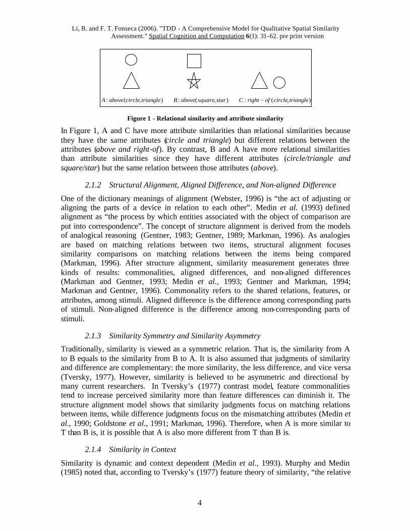
Goldstone et al. (1991) and Medin et al. (1993) deal with the distinction between relational similarity and attribute similarity. An attribute refers to a component or a property of a stimulus. Therefore, the attribute similarity between a pair of stimulus means how similar their attributes are. Whereas the relational similarity of a pair of stimulus refers to how similar the relations of their attributes are. Goldstone gave the following example to illustrate these two concepts.


4

),(: trianglecircleaboveA ),(: starsquareaboveB ),(: trianglecircleofrightC −

Figure 1 - Relational similarity and attribute similarity

In Figure 1, A and C have more attribute similarities than relational similarities because they have the same attributes (circle and triangle) but different relations between the attributes (above and right-of). By contrast, B and A have more relational similarities than attribute similarities since they have different attributes (circle/triangle and square/star) but the same relation between those attributes (above).

2.1.2 Structural Alignment, Aligned Difference, and Non-aligned Difference

One of the dictionary meanings of alignment (Webster, 1996) is “the act of adjusting or aligning the parts of a device in relation to each other”. Medin et al. (1993) defined alignment as “the process by which entities associated with the object of comparison are put into correspondence”. The concept of structure alignment is derived from the models of analogical reasoning (Gentner, 1983; Gentner, 1989; Markman, 1996). As analogies are based on matching relations between two items, structural alignment focuses similarity comparisons on matching relations between the items being compared (Markman, 1996). After structure alignment, similarity measurement generates three kinds of results: commonalities, aligned differences, and non-aligned differences (Markman and Gentner, 1993; Medin et al., 1993; Gentner and Markman, 1994; Markman and Gentner, 1996). Commonality refers to the shared relations, features, or attributes, among stimuli. Aligned difference is the difference among corresponding parts of stimuli. Non-aligned difference is the difference among non-corresponding parts of stimuli.

2.1.3 Similarity Symmetry and Similarity Asymmetry

Traditionally, similarity is viewed as a symmetric relation. That is, the similarity from A to B equals to the similarity from B to A. It is also assumed that judgments of similarity and difference are complementary: the more similarity, the less difference, and vice versa (Tversky, 1977). However, similarity is believed to be asymmetric and directional by many current researchers. In Tversky’s (1977) contrast model, feature commonalities tend to increase perceived similarity more than feature differences can diminish it. The structure alignment model shows that similarity judgments focus on matching relations between items, while difference judgments focus on the mismatching attributes (Medin et al., 1990; Goldstone et al., 1991; Markman, 1996). Therefore, when A is more similar to T than B is, it is possible that A is also more different from T than B is.

2.1.4 Similarity in Context

Similarity is dynamic and context dependent (Medin et al., 1993). Murphy and Medin (1985) noted that, according to Tversky’s (1977) feature theory of similarity, “the relative


5

weighting of a feature varies with the stimulus context and task, so that there is no unique answer to the question of how similar is one object to another”. Goodman (1972) claimed that the similarity of A to B is an ill-defined, meaningless notion unless one can say “in which respects”. In general, the relevant feature space is not explicitly specified but rather inferred from the general context (Tversky, 1977). Due to the separable stimuli, such as figures varying in color and shape, or lines varying in length and orientation, subjects sometimes experience difficulties in evaluating overall similarity and occasionally tend to evaluate similarities with respect to one factor or the other (Shepard, 1964) or change the relative weights of attributes with a change in context (Torgerson, 1965). Moreover, assessment of similarity varies with factors such as processing time and previous experience (Medin et al., 1993). Medin believes that in the structural alignment model, what gets aligned is not fixed a priori but depends on the particular comparison.

2.2 Similarity Models in the Field of Psychology

Four similarity models are broadly accepted in the field of psychology. They are the geometric model, feature-based contrast model, structure alignment model, and the transformation model.

2.2.1 Geometric Model

The geometric model is the dominant model in theoretical similarity analysis (Torgerson, 1965; Tversky, 1977; Goldstone, 2004). This model represents stimuli as points in a multidimensional space and the similarity of stimulus pair is reflected by the vector distance between the two corresponding points in that space (Tversky, 1977; Thomas and Mareschal, 1997; Markman, 2001; Nedas and Egenhofer, 2003; Goldstone, 2004). Naturally, the geometric model obeys the metric axioms of Minimality, Symmetry, and Triangle Inequality (Tversky, 1977; Thomas and Mareschal, 1997; Goldstone, 2004). However, it has been criticized by Tversky (1977) as not being the case with psychological notions of similarity since human similarity judgments violate the above three axioms. Minimality is violated because not all identical objects are equally similar. Complex objects that are identical (e.g. two spaceships) have more similarity than simpler identical objects (e.g. two balls). In the metric space, similarities are the same whatever the order of the comparison is, whereas similarities are believed to be asymmetric and directional. For example, Japanese culture is more similar to Chinese culture than Chinese culture is to Japanese culture since many features of the Japanese culture come from Chinese culture. Triangle inequality can be violated when A (e.g. a lamp) and B (a moon) share an identical feature as both provide light; B (a moon) and C (a ball) share an identical feature as both are round; however A and C share no feature in common (Tversky and Gati, 1982).

2.2.2 Feature-Based Contrast Model

The feature-based contrast model assumes that objects are represented as collections of features, and similarities among objects are expressed as a feature-matching process among common and distinctive features (Tversky, 1977; Markman, 2001; Goldstone, 2004). Similarities of a stimuli pair increase with its commonalities and decreases with its differences. The common features of a stimuli pair are those elements in the intersection of the feature sets. The distinctive features of a stimuli pair are those elements outside of


6

the intersection of the feature sets. In this model, the similarity of a stimuli pair increases with the size of the common features set and decreases with the size of the distinctive features set (Markman, 1993). The similarity of A to B is expressed as a linear function of the common and distinctive features. Tversky claims that feature commonalities tend to increase perceived similarity more than feature differences can diminish it. That is, commonalities get higher weights than differences do.

2.2.3 Structure Alignment Model

The structure alignment model, inspired in analogical reasoning, indicates that similarities come not only from the matching of common and different features, but also from the alignment of features (Markman, 1993; Goldstone, 1998; Goldstone, 2004). Usually, in the comparison of a stimulus pair, the parts of one object must be aligned or placed in correspondence with the parts of the other (Goldstone, 1994). In this model, outputs of a similarity comparison process include commonalities, aligned differences, and non-aligned differences (Markman and Gentner, 1993; Medin et al., 1993; Gentner and Markman, 1994; Markman and Gentner, 1996). It has been widely recognized that similarity comparisons involve structural alignment instead of simple feature matches (Gentner, 1983; Gentner, 1989; Medin et al., 1990; Markman, 1993; Markman and Gentner, 1993; Medin et al., 1993; Gentner and Markman, 1994; Goldstone, 1994). Medin also argued that structure and global consistency are more important in the process of similarity determination than simple local matches. He also pointed out that what gets aligned is not fixed a priori but depends on the particular comparison. Markman (1996) concluded that similarity judgments focus on matching relations between items, while difference judgments focus on mismatching attributes.

2.2.4 Transformation Model

The transformation model measures similarity through the use of transformational distance (Imai, 1977; Hahn and Chater, 1997; Goldstone, 2004). The concept of transformational distance is defined as a function of the complexity required to transform the representation of one stimulus into the representation of another. According to Kolmogorov complexity theory (Goldstone, 2004), given a set of vocabularies, the complexity of a transformation is the shortest length the computer program needs to move from one vocabulary to another. In other words, the similarity between two entities is the smallest number of operations that a computer program needs to transform one entity into the other.

2.3 Spatial Similarity Assessment

Spatial similarity is hard to address because of the numerous constraints of spatial properties and of the complexity of spatial relations. Since it is believed that spatial relations, mainly topology, direction, and distance, capture the essence of a scene’s structure (Bruns and Egenhofer, 1996), most research focus on the similarity assessment of spatial relations. The two dominant approaches adopted in spatial similarity assessment are conceptual neighborhood approach and projection-based approach.

The conceptual neighborhood approach is based on the transformation model, in which similarity is measured according to the distance between two concepts in a network. It


7

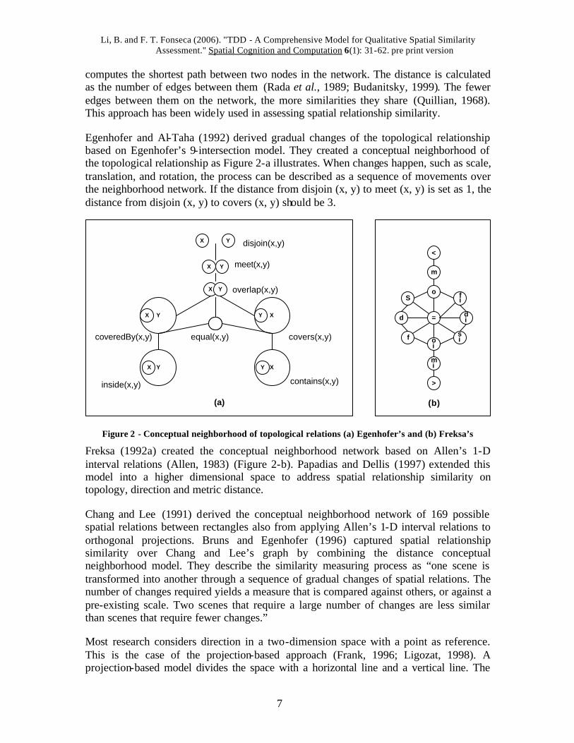
computes the shortest path between two nodes in the network. The distance is calculated as the number of edges between them (Rada et al., 1989; Budanitsky, 1999). The fewer edges between them on the network, the more similarities they share (Quillian, 1968). This approach has been widely used in assessing spatial relationship similarity.

Egenhofer and Al-Taha (1992) derived gradual changes of the topological relationship based on Egenhofer’s 9-intersection model. They created a conceptual neighborhood of the topological relationship as Figure 2-a illustrates. When changes happen, such as scale, translation, and rotation, the process can be described as a sequence of movements over the neighborhood network. If the distance from disjoin (x, y) to meet (x, y) is set as 1, the distance from disjoin (x, y) to covers (x, y) should be 3.

X Y

X Y

X Y

YX XY

YX XY

disjoin(x,y)

meet(x,y)

overlap(x,y)

equal(x,y)coveredBy(x,y)

inside(x,y)

covers(x,y)

contains(x,y)

f

S

si

fi

d di

>

mi

oi

=

o

m

<

(b)(a)

Figure 2 - Conceptual neighborhood of topological relations (a) Egenhofer’s and (b) Freksa’s

Freksa (1992a) created the conceptual neighborhood network based on Allen’s 1-D interval relations (Allen, 1983) (Figure 2-b). Papadias and Dellis (1997) extended this model into a higher dimensional space to address spatial relationship similarity on topology, direction and metric distance.

Chang and Lee (1991) derived the conceptual neighborhood network of 169 possible spatial relations between rectangles also from applying Allen’s 1-D interval relations to orthogonal projections. Bruns and Egenhofer (1996) captured spatial relationship similarity over Chang and Lee’s graph by combining the distance conceptual neighborhood model. They describe the similarity measuring process as “one scene is transformed into another through a sequence of gradual changes of spatial relations. The number of changes required yields a measure that is compared against others, or against a pre-existing scale. Two scenes that require a large number of changes are less similar than scenes that require fewer changes.”

Most research considers direction in a two-dimension space with a point as reference. This is the case of the projection-based approach (Frank, 1996; Ligozat, 1998). A projection-based model divides the space with a horizontal line and a vertical line. The


8

two lines represent the 4 directions: north, west, south, and east. The regions between these two lines represent the secondary directions: northwest, southwest, southeast, and northeast. It was argued that the projection model has advantages over the cone model (Frank, 1991) in implementation due to the rectangular nature of the directional partition (Goyal, 2000).

The projection-based approach projects spatial objects and their relations onto another space, which can be a vector space or a matrix space. This way the problem of similarity assessment shifts from the comparison of objects in spatial scenes to that vector or matrix space. The famous 2D String symbolic representation is an example of projection-based approach (Chang et al., 1987), in which spatial objects and their relationships are represented by 2D strings along x and y axes. The similarity assessment between two scenes is then treated as it was a string matching. Chang defines three types of similarity criteria, type-0, type-1 and type-2. Type-0 is the most generous one. It is fulfilled when two objects have the same relationship on either the x- or the y-axis. Type-1 requires that two objects have the same relations on both the x- and y-axis. Type-2 requires not only two objects to have the same relations but also that they have the same rank of the relative positions.

Goyal and Egenhofer (2001) combines the conceptual neighborhood approach and the projection-based approach for distance similarity measurement. In their work, the directional space is projected into a 3*3 matrix, which represents the nine directions (north, northwest, west, southwest, south, southeast, east, northeast, and same). Each sector of the matrix specifies how much of a target object falls into the direction it represents. The similarity of a cardinal direction is determined by the least cost of transforming one direction-relation matrix into another.

Because of the focus of our work, in this review we reviewed more work on the terminological and psychological than on the spatial aspects of similarity. Nevertheless is worth mentioning that research in spatial similarity range from assessment (Holt and G.L.Benwell, 1997; Bishr, 1998; Holt, 1999; Rodríguez et al., 1999; Rodríguez and Egenhofer, 2003; Rodríguez and Egenhofer, 2004) to qualitative spatial reasoning (Dutta, 1989; Freksa, 1992b; Cohn and Hazarika, 2001; Renz, 2002b), topological relationships (Egenhofer and Franzosa, 1991; Randell et al., 1992; Egenhofer, 1993; Egenhofer, 1994; Egenhofer et al., 1994; Egenhofer and Franzosa, 1995; Cohn and Varzi, 1998; Cohn and Varzi, 1999), directional relationships (Hernandez, 1994; Frank, 1996; Ligozat, 1998; Goyal and Egenhofer, 2000; Cohn and Hazarika, 2001; Renz, 2002b), metric distance (Clementini et al., 1994; Hernandez et al., 1995; Cohn and Hazarika, 2001; Renz, 2002b), conceptual neighborhood approach (Allen, 1983; Rada et al., 1989; Egenhofer and Al-Taha, 1992; Freksa, 1992a; Papadias and Dellis, 1997; Budanitsky, 1999), and projection-based approach (Chang et al., 1987; Papadias et al., 1999; Goyal and Egenhofer, 2001).


9

3 The TDD Model to Measure Similarity between Spatial Scenes

Our model provides a similarity measure that integrates four widely accepted conceptual similarity models which are the geometric model, the feature contrast model, the transformation model, and the structure alignment model. It measures both commonalities (C) and differences (D) between spatial scenes. The final similarity measurement (S) is a combination of both, S = C - D. The structure alignment model considers that in the comparison of a stimulus pair, the parts of one object must be aligned or placed in correspondence with the parts of the other. Therefore, the output of the similarity comparison process includes commonalities, alignable differences, and non-alignable differences. Our model treats alignable differences and non-alignable differences separately, D = (alignable difference + non alignable difference).

Our model addresses both relational similarity and attributes similarity (Table 1). Considering that relational similarity and attribute similarity have different impacts on the commonality judgment and difference judgment (Tversky, 1977), different weights might be applied on them in similarity evaluation of a certain task context.

Sometimes the similarity of object A in relation to object B is different from the similarity of B in relation to A (Tversky, 1977). This situation is called similarity asymmetry. It is a context-dependent issue. Depending on the task context, different attributes or relations will have more or less relevance in the similarity evaluation. Our solution to address this problem is to have different weights associated with each attribute and each relation. Users of our model may set the weights interactively so that they reflect the particular situation in which the similarity measurement is being made.

Other contributions of our model include applying the order of priority topology à direction à distance into spatial similarity assessment and the relaxation of the transformation cost. Both features are implemented through the weight setting. The details are discussed later in this section.

In order to be able to take an initial step in the implementation of our model we opted to limit our scope. In this work we deal only with scenes with two objects. Therefore, spatial distribution is not measured. Another limitation refers to the three levels of spatial similarity addressed by Rodriguez et al. (1999). In our model we deal with the geometric and the thematic levels only. We leave the semantic level for future work.

Another interesting question that we left out is the combination of topology and the metric characteristics of the spatial objects under consideration. For instance, consider the case in two scenes with both having two objects separated by distances that are largely different. Consider also that although the distances highly differ in their absolute value they still are proportional to the objects’ sizes. Godoy and Rodriguez (2004) consider explicitly the relation of metric measurements and topological relations showing its importance in the evaluation of similarity.


10

Next we will analyze the basic spatial similarity elements addressed by our model; explain the similarity alignment in which this model is based on; and finally introduce the similarity measurement that this model applies.

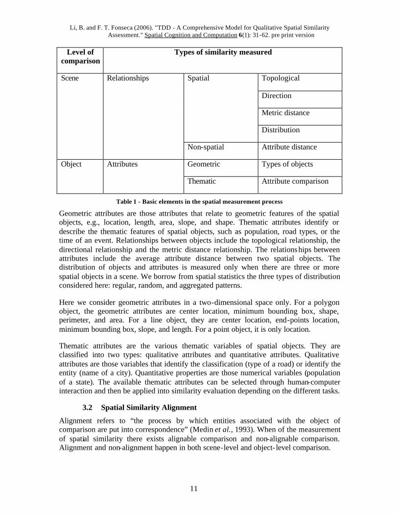
3.1 Spatial Similarity Elements

Our model measures the similarity between spatial scenes. A spatial scene is comprised of spatial objects. We consider three different types of spatial objects: a point, such as a city or a factory, a line, such as a road or a river, and a polygon, such as a state or a county. The types of spatial scenes we address in our model are (1) scenes with only one spatial object in it, (2) scenes with two spatial objects in it, and (3) scenes with three or more spatial objects in it. A scene with a single spatial object is the simplest type of stimulus. For instance, in the query ‘finding the states that are similar to Georgia’ each state in the U. S. is considered a scene with one spatial object (the state boundary itself). Since there is only one object in each scene, no relational similarity is evaluated. Geometric and thematic attributes of each state are compared with those of Georgia in the similarity assessment process. In the case of scenes with two spatial objects, then, besides the geometric and thematic attributes of each spatial object, the spatial relationships between objects in each scene and the attribute-distance relationships between these two spatial objects are also measured. Similarity evaluation for scenes with three or more spatial objects is more complex. It is necessary to measure also the distribution of objects and attributes besides measuring the similarity between geometric and thematic attributes.

A spatial scene may be composed of one or more layers. For instance, a scene describing the distribution of population and water in Pennsylvania may include a layer with administrative boundaries such as counties, and a hydrology layer with rivers and lakes. In addressing similarity of such scenes, besides scene- level comparison, there is also layer- level comparison. Scene-level comparison investigates the overall relationships of each scene. In layer- level comparison we are interested in comparing objects in each layer of the scenes. Comparisons at this level would include the geometric attributes (e.g., the type of spatial object, location, area, and length) and thematic attributes (e.g., population and income). We call the similarity measured in scene- level comparison relational similarity and we call the similarity measured at the layer- level object similarity. Therefore, regarding the measurement itself, we consider two levels in our model. One is the scene level and the other, related to layers, is the object level. At the scene level we are interested in finding and measuring relationships. At the object level we are interested in measuring attributes. The relationships are further divided into spatial relationships and non-spatial relationships. The attributes are classified as geometric and thematic attributes (Table 1).


11

Level of comparison

Types of similarity measured

Topological

Direction

Metric distance

Spatial

Distribution

Scene Relationships

Non-spatial Attribute distance

Geometric Types of objects Object Attributes

Thematic Attribute comparison

Table 1 - Basic elements in the spatial measurement process

Geometric attributes are those attributes that relate to geometric features of the spatial objects, e.g., location, length, area, slope, and shape. Thematic attributes identify or describe the thematic features of spatial objects, such as population, road types, or the time of an event. Relationships between objects include the topological relationship, the directional relationship and the metric distance relationship. The relationships between attributes include the average attribute distance between two spatial objects. The distribution of objects and attributes is measured only when there are three or more spatial objects in a scene. We borrow from spatial statistics the three types of distribution considered here: regular, random, and aggregated patterns.

Here we consider geometric attributes in a two-dimensional space only. For a polygon object, the geometric attributes are center location, minimum bounding box, shape, perimeter, and area. For a line object, they are center location, end-points location, minimum bounding box, slope, and length. For a point object, it is only location.

Thematic attributes are the various thematic variables of spatial objects. They are classified into two types: qualitative attributes and quantitative attributes. Qualitative attributes are those variables that identify the classification (type of a road) or identify the entity (name of a city). Quantitative properties are those numerical variables (population of a state). The available thematic attributes can be selected through human-computer interaction and then be applied into similarity evaluation depending on the different tasks.

3.2 Spatial Similarity Alignment

Alignment refers to “the process by which entities associated with the object of comparison are put into correspondence” (Medin et al., 1993). When of the measurement of spatial similarity there exists alignable comparison and non-alignable comparison. Alignment and non-alignment happen in both scene-level and object- level comparison.


12

In scene- level comparison, two stimuli (scenes) are alignable if they are the same type of scenes, and are non-alignable if they are different type of scenes. For example, a scene with one object is non-alignable with a scene with two objects; a scene with two objects is alignable with another scene with two objects. It is important to note that scene- level alignment should not be considered as simple as the alignment of the same number of objects. Scene- level comparison investigates the overall relationships of each scene. Scenes with different number of objects are different because these scenes may differ greatly in terms of spatial relationships and spatial distribution although not being that much different in terms of the number of objects.

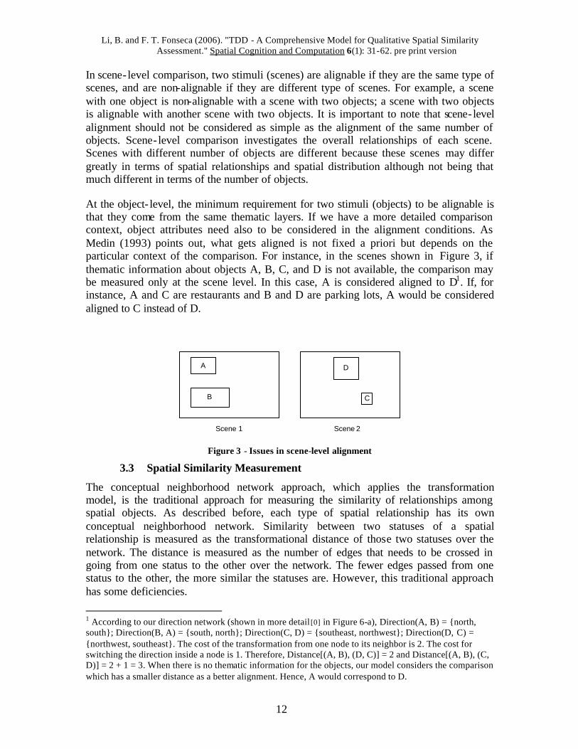
At the object- level, the minimum requirement for two stimuli (objects) to be alignable is that they come from the same thematic layers. If we have a more detailed comparison context, object attributes need also to be considered in the alignment conditions. As Medin (1993) points out, what gets aligned is not fixed a priori but depends on the particular context of the comparison. For instance, in the scenes shown in Figure 3, if thematic information about objects A, B, C, and D is not available, the comparison may be measured only at the scene level. In this case, A is considered aligned to D1. If, for instance, A and C are restaurants and B and D are parking lots, A would be considered aligned to C instead of D.

A

B

Scene 1

D

C

Scene 2

Figure 3 - Issues in scene-level alignment

3.3 Spatial Similarity Measurement

The conceptual neighborhood network approach, which applies the transformation model, is the traditional approach for measuring the similarity of relationships among spatial objects. As described before, each type of spatial relationship has its own conceptual neighborhood network. Similarity between two statuses of a spatial relationship is measured as the transformational distance of those two statuses over the network. The distance is measured as the number of edges that needs to be crossed in going from one status to the other over the network. The fewer edges passed from one status to the other, the more similar the statuses are. However, this traditional approach has some deficiencies.

1 According to our direction network (shown in more detail [0] in Figure 6-a), Direction(A, B) = {north, south}; Direction(B, A) = {south, north}; Direction(C, D) = {southeast, northwest}; Direction(D, C) = {northwest, southeast}. The cost of the transformation from one node to its neighbor is 2. The cost for switching the direction inside a node is 1. Therefore, Distance[(A, B), (D, C)] = 2 and Distance[(A, B), (C, D)] = 2 + 1 = 3. When there is no thematic information for the objects, our model considers the comparison which has a smaller distance as a better alignment. Hence, A would correspond to D.


13

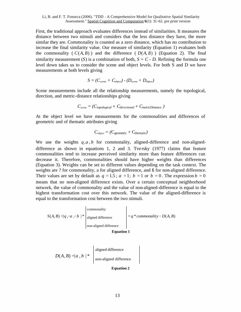
First, the traditional approach evaluates differences instead of similarities. It measures the distance between two stimuli and considers that the less distance they have, the more similar they are. Commonality is counted as a zero distance, which has no contribution to increase the final similarity value. Our measure of similarity (Equation 1) evaluates both the commonality ( ),( BAC ) and the difference ( ),( BAD ) (Equation 2). The final similarity measurement (S) is a combination of both, S = C - D. Refining the formula one level down takes us to consider the scene and object levels. For both S and D we have measurements at both levels giving

S = (Cscene + Cobject) - (Dscene + Dobject)

Scene measurements include all the relationship measurements, namely the topological, direction, and metric-distance relationships giving

Cscene = (Ctopological + Cdirectional + CmetricDistance )

At the object level we have measurements for the commonalities and differences of geometric and of thematic attributes giving

Cobject = (Cgeometric + Cthematic)

We use the weights βαθ ,, for commonality, aligned-difference and non-aligned-difference as shown in equations 1, 2 and 3. Tve rsky (1977) claims that feature commonalities tend to increase perceived similarity more than feature differences can decrease it. Therefore, commonalities should have higher weights than differences (Equation 3). Weights can be set to different values depending on the task context. The weights are ? for commonality, a for aligned difference, and ß for non-aligned difference. Their values are set by default as 5.1=θ ; 1=α ; 1=β or 0=β . The expression 0=β means that no non-aligned difference exists. Over a certain conceptual neighborhood network, the value of commonality and the value of non-aligned-difference is equal to the highest transformation cost over this network. The value of the aligned-difference is equal to the transformation cost between the two stimuli.

∗−−= |,,|),( βαθBAS

commonality

aligned difference

non-aligned difference

),(* BADycommonalit −= θ

Equation 1

∗= |,|),( βαBADaligned difference

non-aligned difference

Equation 2


14

αθ > , βθ > (By default: 5.1=θ ; 1=α ; 1=β or 0=β )

Equation 3

The second deficiency of the traditional approach is that the three types of spatial relationships (topological, direction and metric distance) are treated with the same priority. However, when children acquire the spatial notions, the order is topology ? direction ? metric distance, in which topology affects the acquisition of spatial notions most and metric distance affects it the least (Renz, 2002a). Therefore, to be consistent with spatial cognition, the order is topology ? direction ? metric distance. In this case, topology affects the acquisition of spatial notions the most and metric distance affects it the least. Therefore, our work on similarity assessment takes this order into account. The strategy that we adopted here is to reflect that order by setting weights of transformation costs on the three types of spatial relationship differently as Equation 4 shows. The default values for weights are 3:2:1 corresponding to

tance)weight(disection)weight(dirology)weight(top >> By default: 3:2:1distance)t(metricion):weighght(directology):weiweight(top =⋅

Equation 4

Finally, the traditional approach counts the number of edges from one status to another status over the network as the distance between these two statuses. This method of computation assumes that each edge represents the same distance. However, over the topological conceptual neighborhood network, the distances represented by each edge are different. We refine the solution of this problem by grouping the topological relationships and proposing the concepts of inter- and intra-group transformation costs on the edges of the conceptual neighborhood network. The model of transformation cost can be described as Cost (inter group) > Cost (intra group) > Cost (intra sub group).

group)sub(intraCost group)(intraCost group)(interCost >>

By default: 1:2:3 group)sub(intraCost : group)(intraCost : group)(interCost =

Equation 5

Our model is described by the above equations. We discuss next the details of how our model deals with the similarity of topological, directional, metric-distance relationships and the two type of attributes (geometric and thematic).

4 Measuring the Similarity of Spatial Relationships As shown in Table 1, the similarity measurements taken into the consideration by the model are related to relationships and attributes. In this section we give the details of the relationship measurements (topological, directional, and metric-distance). The two attribute measurements (geometric and thematic) are discussed in the section that deals with the computational implementation.


15

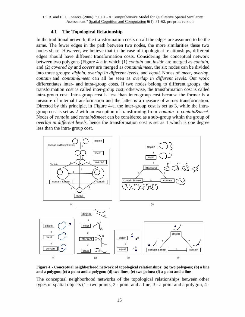
4.1 The Topological Relationship

In the traditional network, the transformation costs on all the edges are assumed to be the same. The fewer edges in the path between two nodes, the more similarities these two nodes share. However, we believe that in the case of topological relationships, different edges should have different transformation costs. Considering the conceptual network between two polygons (Figure 4-a in which (1) contain and inside are merged as contain, and (2) covered by and covers are merged as contain&meet, the six nodes can be divided into three groups: disjoin, overlap in different levels, and equal. Nodes of meet, overlap, contain and contain&meet can all be seen as overlap in different levels. Our work differentiates inter- and intra-group costs. If two nodes belong to different groups, the transformation cost is called inter-group cost; otherwise, the transformation cost is called intra-group cost. Intra-group cost is less than inter-group cost because the former is a measure of internal transformation and the latter is a measure of across transformation. Directed by this principle, in Figure 4-a, the inter-group cost is set as 3, while the intra-group cost is set as 2 with an exception of transforming from contain to contain&meet. Nodes of contain and contain&meet can be considered as a sub-group within the group of overlap in different levels, hence the transformation cost is set as 1 which is one degree less than the intra-group cost.

(a) (b)

(c) (d) (e) (f)

3

equal

disjoin

2

meet

overlap

33

Overlap in different levels:

containcontain & meet

2 2

31

Contain:

disjoin

meet

intersect

contain & meet contain1

3

2

22

disjoin

meet

contain

3

4

disjoin

A, B

A

B

AB

intersect

equal

meet

B

A

3

2

3

A

A

B

Bdisjoin

equal

8

disjoin

contain & meet contain

77

1

Figure 4 - Conceptual neighborhood network of topological relationships: (a) two polygons; (b) a line and a polygon; (c) a point and a polygon; (d) two lines; (e) two points; (f) a point and a line

The conceptual neighborhood networks of the topological relationships between other types of spatial objects (1 - two points, 2 - point and a line, 3 - a point and a polygon, 4 -


16

two lines, and 5 - a line and a polygon) are derived using the schemas shown in Figure 4-a. The derivation principle is as following. First, duplicate the topological relationship model between two polygons no matter what types of spatial objects the scene has. Second, cut off the duplication and the impossible nodes and edges connected with them. For example, in the relationship between a point and a polygon, in Figure 4-c, overlap and contain&meet between a point and a polygon are duplications of meet. Moreover, it is not possible to have an equal topology between a point and a polygon. Third, apply the transformation cost. When two edges merge into one edge because of duplication, the weight for the final edge is the sum of the original two. For the path from meet to contain, in Figure 4-a, there are two edges with weight of 2 on each of them; however in Figure 4-c, overlap is cut off and there is only one edge left with the weight of 422 =+ .

4.2 The Directional Relationship

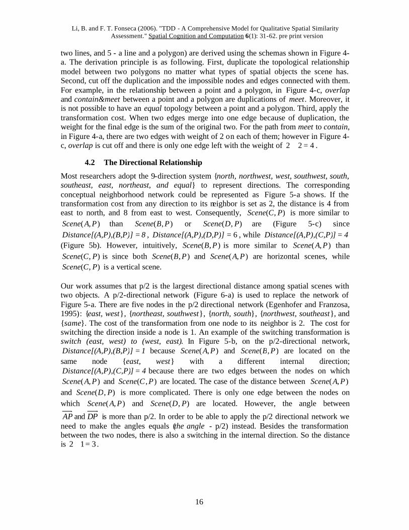
Most researchers adopt the 9-direction system {north, northwest, west, southwest, south, southeast, east, northeast, and equal} to represent directions. The corresponding conceptual neighborhood network could be represented as Figure 5-a shows. If the transformation cost from any direction to its neighbor is set as 2, the distance is 4 from east to north, and 8 from east to west. Consequently, ),( PCScene is more similar to

),( PAScene than ),( PBScene or ),( PDScene are (Figure 5-c) since 8]A,P),(B,P)Distance[( = , 6=]A,P),(D,P)Distance[( , while 4]A,P),(C,P)Distance[( =

(Figure 5b). However, intuitively, ),( PBScene is more similar to ),( PAScene than ),( PCScene is since both ),( PBScene and ),( PAScene are horizontal scenes, while ),( PCScene is a vertical scene.

Our work assumes that p/2 is the largest directional distance among spatial scenes with two objects. A p/2-directional network (Figure 6-a) is used to replace the network of Figure 5-a. There are five nodes in the p/2 directional network (Egenhofer and Franzosa, 1995): {east, west}, {northeast, southwest}, {north, south}, {northwest, southeast}, and {same}. The cost of the transformation from one node to its neighbor is 2. The cost for switching the direction inside a node is 1. An example of the switching transformation is switch (east, west) to (west, east). In Figure 5-b, on the p/2-directional network,

1]A,P),(B,P)Distance[( = because ),( PAScene and ),( PBScene are located on the same node {east, west} with a different internal direction;

4]A,P),(C,P)Distance[( = because there are two edges between the nodes on which ),( PAScene and ),( PCScene are located. The case of the distance between ),( PAScene

and ),( PDScene is more complicated. There is only one edge between the nodes on which ),( PAScene and ),( PDScene are located. However, the angle between

AP and DP is more than p/2. In order to be able to apply the p/2 directional network we need to make the angles equals (the angle - p/2) instead. Besides the transformation between the two nodes, there is also a switching in the internal direction. So the distance is 312 =+ .


17

(b)(a)

(c)

NW

SESW S

W E

NEN

22

2

22

2

2

2

Orientation(A,P) = {east}Orientation(B,P) = {west}Orientation(C,P) = {north}Orientation(D,P)={northwest}

Distance [(A,P), (B,P)] = 8Distance [(A,P), (C,P)] =4Distance [(A,P), (D,P)] = 6

AB

C

P

D

B

AP P

C

P P

D

4 6 8

Figure 5 - (a) Traditional direction network; (b) pattern examples; (c) ranking of similarity for the patterns in (b)

(a) (b)

(c)

W E

S

NSW

NE

NW

SE

22

22

1

1

1

1same 2

2

2

2

BA

P P

C

PP

D

431

Orientation(A,P) = (east, west)Orientation(B,P) = (west, east)Orientation(C,P) = (north, south)Orientation(D,P) = (northwest,southwest)

Distance [(A,P), (B,P)] = 1Distance [(A,P), (C,P)] = 4Distance [(A,P), (D,P)] = 3

AB

C

P

D

Figure 6 - (a) direction network; (b) pattern examples; (c) ranking of similarity for the patterns in (b)

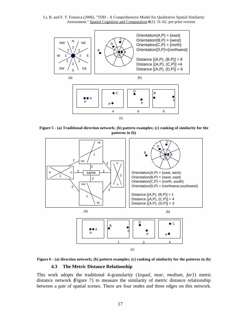
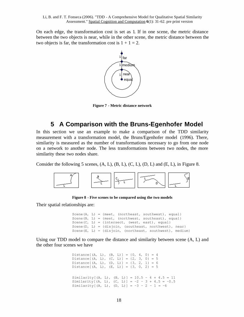
4.3 The Metric Distance Relationship

This work adopts the traditional 4-granularity ({equal, near, medium, far}) metric distance network (Figure 7) to measure the similarity of metric distance relationship between a pair of spatial scenes. There are four nodes and three edges on this network.


18

On each edge, the transformation cost is set as 1. If in one scene, the metric distance between the two objects is near, while in the other scene, the metric distance between the two objects is far, the transformation cost is 1 + 1 = 2.

1

1

equalnear

medium

far1

Figure 7 - Metric distance network

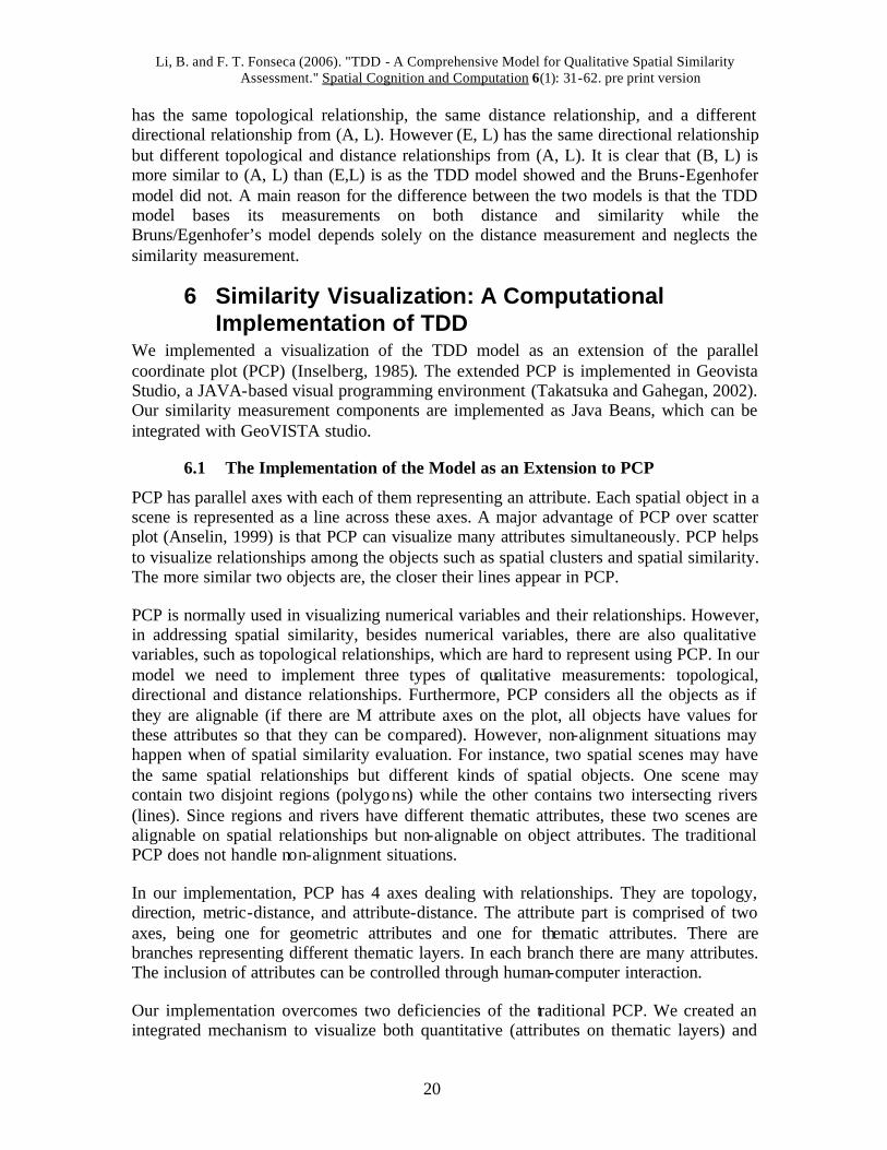
5 A Comparison with the Bruns-Egenhofer Model In this section we use an example to make a comparison of the TDD similarity measurement with a transformation model, the Bruns/Egenhofer model (1996). There, similarity is measured as the number of transformations necessary to go from one node on a network to another node. The less transformations between two nodes, the more similarity these two nodes share.

Consider the following 5 scenes, (A, L), (B, L), (C, L), (D, L) and (E, L), in Figure 8.

Figure 8 - Five scenes to be compared using the two models

Their spatial relationships are:

Scene(A, L) = {meet, (northeast, southwest), equal} Scene(B, L) = {meet, (northwest, southeast), equal} Scene(C, L) = {intersect, (west, east), equal} Scene(D, L) = {disjoin, (southeast, northwest), near} Scene(E, L) = {disjoin, (northeast, southwest), medium}

Using our TDD model to compare the distance and similarity between scene (A, L) and the other four scenes we have

Distance[(A, L), (B, L)] = {0, 4, 0} = 4 Distance[(A, L), (C, L)] = {2, 3, 0} = 5 Distance[(A, L), (D, L)] = {3, 2, 1} = 6 Distance[(A, L), (E, L)] = {3, 0, 2} = 5 Similarity[(A, L), (B, L)] = 10.5 – 4 + 4.5 = 11 Similarity[(A, L), (C, L)] = -2 – 3 + 4.5 = -0.5 Similarity[(A, L), (D, L)] = -3 – 2 - 1 = -6


19

Distance[(A, L), (E, L)] = -3 + 6 – 2 = 1

giving the following similarity ranking (Figure 9) from most similar to least similar: (B, L), (E, L), (C, L), and (D, L).

Figure 9 - Result of the comparison using the TDD model

The similarity measurement in the Bruns/Egenhofer’s model has a different result from the TDD model. In Figure 10 we can see which nodes represent these five scenes.

Figure 10 - The five scenes in the Bruns-Egenhofer model

By calculating the number of transformations from (A, L) to the other four scenes, we have the distance measurement as follows

Distance[(A, L), (B, L)] = 3 Distance[(A, L), (C, L)] = 3 Distance[(A, L), (D, L)] = 5 Distance[(A, L), (E, L)] = 1

Therefore, the similarity ranking based on the Bruns/Egenhofer’s model from most similar to least similar is (E, L), (C, L)/(B, L), and (D, L). There are some differences in the results from the two models. If we compare (B, L) and (E, L), we can see that (B, L)


20

has the same topological relationship, the same distance relationship, and a different directional relationship from (A, L). However (E, L) has the same directional relationship but different topological and distance relationships from (A, L). It is clear that (B, L) is more similar to (A, L) than (E,L) is as the TDD model showed and the Bruns-Egenhofer model did not. A main reason for the difference between the two models is that the TDD model bases its measurements on both distance and similarity while the Bruns/Egenhofer’s model depends solely on the distance measurement and neglects the similarity measurement.

6 Similarity Visualization: A Computational Implementation of TDD

We implemented a visualization of the TDD model as an extension of the parallel coordinate plot (PCP) (Inselberg, 1985). The extended PCP is implemented in Geovista Studio, a JAVA-based visual programming environment (Takatsuka and Gahegan, 2002). Our similarity measurement components are implemented as Java Beans, which can be integrated with GeoVISTA studio.

6.1 The Implementation of the Model as an Extension to PCP

PCP has parallel axes with each of them representing an attribute. Each spatial object in a scene is represented as a line across these axes. A major advantage of PCP over scatter plot (Anselin, 1999) is that PCP can visualize many attributes simultaneously. PCP helps to visualize relationships among the objects such as spatial clusters and spatial similarity. The more similar two objects are, the closer their lines appear in PCP.

PCP is normally used in visualizing numerical variables and their relationships. However, in addressing spatial similarity, besides numerical variables, there are also qualitative variables, such as topological relationships, which are hard to represent using PCP. In our model we need to implement three types of qualitative measurements: topological, directional and distance relationships. Furthermore, PCP considers all the objects as if they are alignable (if there are M attribute axes on the plot, all objects have values for these attributes so that they can be compared). However, non-alignment situations may happen when of spatial similarity evaluation. For instance, two spatial scenes may have the same spatial relationships but different kinds of spatial objects. One scene may contain two disjoint regions (polygons) while the other contains two intersecting rivers (lines). Since regions and rivers have different thematic attributes, these two scenes are alignable on spatial relationships but non-alignable on object attributes. The traditional PCP does not handle non-alignment situations.

In our implementation, PCP has 4 axes dealing with relationships. They are topology, direction, metric-distance, and attribute-distance. The attribute part is comprised of two axes, being one for geometric attributes and one for thematic attributes. There are branches representing different thematic layers. In each branch there are many attributes. The inclusion of attributes can be controlled through human-computer interaction.

Our implementation overcomes two deficiencies of the traditional PCP. We created an integrated mechanism to visualize both quantitative (attributes on thematic layers) and


21

qualitative (relationships) data. We use branched parallel-coordinates to handle the non-alignment problem in similarity assessment. Spatial objects are represented as lines across the visualization panel. If two lines go to different branches, the segments on the different branches are non-alignable. For example, in Figure 8, the two lines are alignable on both the scene-part and the object-part, except for one branch representing attributes 21, 22, and 23 which are present only for the dotted line.

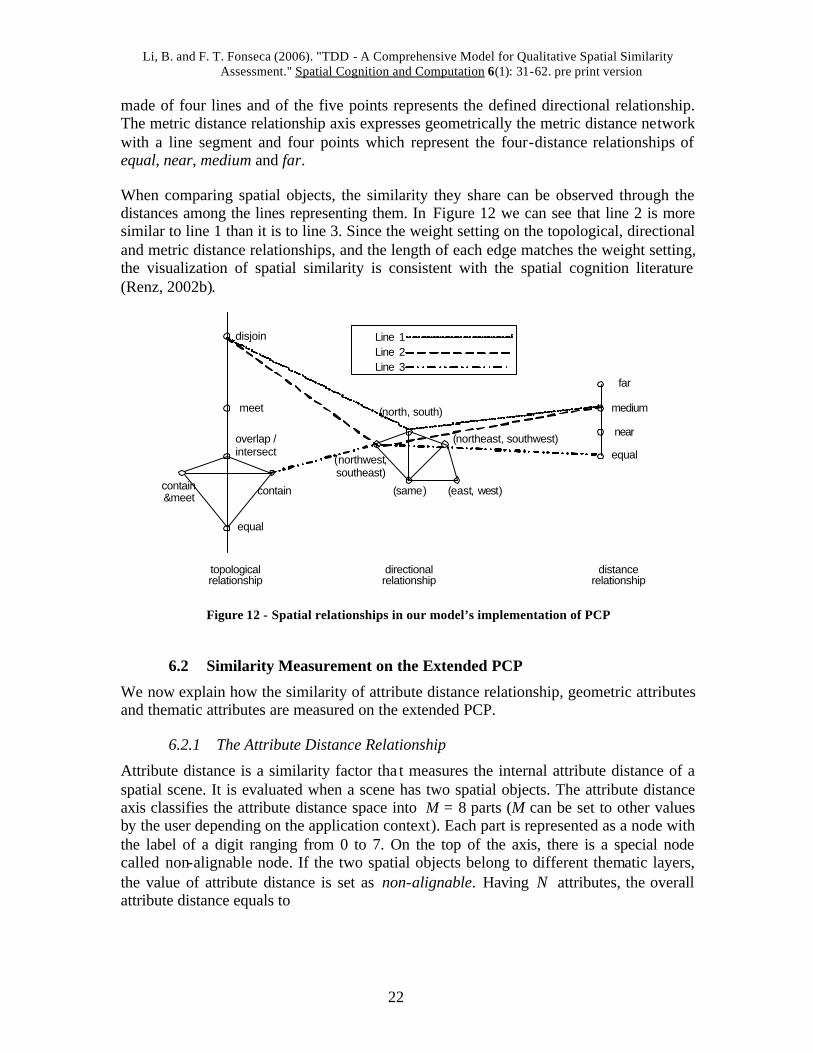
Figure 11 - Detail of the implementation of the model

In order to visualize the qualitative spatial relationships, the traditional PCP vertical axis is replaced in the implementation of our model by a conceptual neighborhood network. On the topological relationship axis, six nodes represent different types of topological relationships which are disjoin, meet, overlap (or intersect), contain, contain&meet, and equal. The lengths of the edges on the axis between the nodes reflect the weight setting defined in the topological network. The relationship between the weight setting of each edge and the metric length of each edge on the axis can be described as

distance2metricdistance1metric

weightweight

=21

An exception is the edge from contain to contain&meet. The weight of the edge from contain to contain&meet is 1; from overlap/intersect to the other nodes is 2; from equal to the other nodes is 3. However, this weight relationship could not be geometrically represented due to the rule that, in a triangle, the sum of two edges is more than the third edge.

On the direction network the five relationships are east west, northeast southwest , north south, northwest southeast, and same. The weight setting for each edge is 2. The figure

disjoin

meet

overlap

containcontain&meet

equal

(northeast, southwest )

(east, west)

(north, south)

(northwest, southeast)

(same) equal

near

medium

far

Topology DirectionMetric

Distance

point

line

polygon

Attribute 11 Attribute 12 Attribute 13



Geometric Thematic

Object -part

0

1

2

3

4

5

6

7

Attribute Distance

non-alignableScene-part


22

made of four lines and of the five points represents the defined directional relationship. The metric distance relationship axis expresses geometrically the metric distance network with a line segment and four points which represent the four-distance relationships of equal, near, medium and far.

When comparing spatial objects, the similarity they share can be observed through the distances among the lines representing them. In Figure 12 we can see that line 2 is more similar to line 1 than it is to line 3. Since the weight setting on the topological, directional and metric distance relationships, and the length of each edge matches the weight setting, the visualization of spatial similarity is consistent with the spatial cognition literature (Renz, 2002b).

disjoin

meet

overlap / intersect

containcontain&meet

equal

(northeast, southwest)

(east, west)

(north, south)

(northwest, southeast)

(same)

equal

near

medium

far

topological relationship

directional relationship

distance relationship

Line 1Line 2Line 3

Figure 12 - Spatial relationships in our model’s implementation of PCP

6.2 Similarity Measurement on the Extended PCP

We now explain how the similarity of attribute distance relationship, geometric attributes and thematic attributes are measured on the extended PCP.

6.2.1 The Attribute Distance Relationship

Attribute distance is a similarity factor tha t measures the internal attribute distance of a spatial scene. It is evaluated when a scene has two spatial objects. The attribute distance axis classifies the attribute distance space into M = 8 parts (M can be set to other values by the user depending on the application context). Each part is represented as a node with the label of a digit ranging from 0 to 7. On the top of the axis, there is a special node called non-alignable node. If the two spatial objects belong to different thematic layers, the value of attribute distance is set as non-alignable. Having N attributes, the overall attribute distance equals to


23

N

distanceattributeN

1ii∑

=

The attribute distance of two values ( 21 ,valuevalue ) on the thi attribute is calculated as

valueminvaluemax

valuevalueabsMath 21

−

−

In order to divide the attribute distance space into M parts

jdistanceattribute i = , )1

minmax( 21

Mj

valuevalue

valuevalueabsMath

Mj

if+

<−

−≤ , 1,...2,1,0 −= Mj .

Considering two scenes, scene1 and scene2, if the overall attribute distance of scene1 ( )1(SceneD ) equals to the overall attribute distance of scene2 ( )2(SceneD ),

Mene2)(Scene1,Scsimilaritydistanceattribute = ;

otherwise, D(Scene2)|e1)abs|D(ScenMathene2)(Scene1,Scsimilaritydistanceattribute −−= .

6.2.2 The Geometric Attributes

On the geometric attribute axis, it is the number of common types of spatial objects that is measured as commonality and difference. Given two scenes, let M to be the set of spatial object types in scene1 ( },,{ polygonlinetpoinM ⊆ ); let N to be the set of spatial-object types in scene2 ( },,{ polygonlinetpoinN ⊆ ); NMC ∧= ( },,{ polygonlinetpoinC ⊆ ) is the set of common spatial object types and NumberOf (C) is the number of common spatial object types in comparison of two scenes.

NMNMP ∧−∨= ( },,{ polygonlinetpoinP ⊆ ) is the set of different spatial-object types and NumberOf (P) is the number of different spatial-object types in the comparison of two scenes. Let the weighted distance range to be {0, MAX},

MAXNMNumNMNum

cycommonalitweighted *)()('

∨∧

==

MAXNMNum

PNumddifferenceweighted *

)()('

∨== ,

''*5.1 dcsimilarityweighted −= ,

)( NMNum ∨ = the number of spatial-object types in the set of NM ∨ .


24

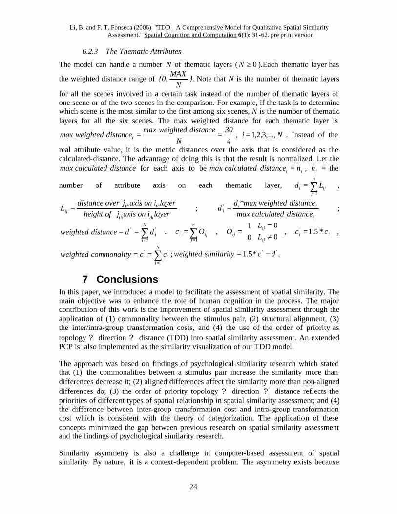
6.2.3 The Thematic Attributes

The model can handle a number N of thematic layers ( 0≥N ).Each thematic layer has

the weighted distance range of {0,N

MAX}. Note that N is the number of thematic layers

for all the scenes involved in a certain task instead of the number of thematic layers of one scene or of the two scenes in the comparison. For example, if the task is to determine which scene is the most similar to the first among six scenes, N is the number of thematic layers for all the six scenes. The max weighted distance for each thematic layer is

430

Nncedistaweightedmax

ncedistaweightedmax i == , Ni ,...,3,2,1= . Instead of the

real attribute value, it is the metric distances over the axis that is considered as the calculated-distance. The advantage of doing this is that the result is normalized. Let the

distancecalculatedmax for each axis to be ii ndistancecalculatedmax = , in = the

number of attribute axis on each thematic layer, ∑=

=n

jiji Ld

1

,

layerionaxisjofheightlayerionaxisjoverdistance

Lthth

ththij = ;

i

iii distancecalculatedmax

distanceweighted*maxdd =' ;

∑=

==N

1i

'i

' dddistanceweighted . ∑=

=n

jiji Oc

1

, 00

01

≠=

=ij

ijij L

LO , ii cc *5.1' = ,

∑=

==N

iiccycommonalitweighted

1

'' ; ''*5.1 dcsimilarityweighted −= .

7 Conclusions In this paper, we introduced a model to facilitate the assessment of spatial similarity. The main objective was to enhance the role of human cognition in the process. The major contribution of this work is the improvement of spatial similarity assessment through the application of (1) commonality between the stimulus pair, (2) structural alignment, (3) the inter/intra-group transformation costs, and (4) the use of the order of priority as topology ? direction ? distance (TDD) into spatial similarity assessment. An extended PCP is also implemented as the similarity visualization of our TDD model.

The approach was based on findings of psychological similarity research which stated that (1) the commonalities between a stimulus pair increase the similarity more than differences decrease it; (2) aligned differences affect the similarity more than non-aligned differences do; (3) the order of priority topology ? direction ? distance reflects the priorities of different types of spatial relationship in spatial similarity assessment; and (4) the difference between inter-group transformation cost and intra-group transformation cost which is consistent with the theory of categorization. The application of these concepts minimized the gap between previous research on spatial similarity assessment and the findings of psychological similarity research.

Similarity asymmetry is also a challenge in computer-based assessment of spatial similarity. By nature, it is a context-dependent problem. The asymmetry exists because


25

the context of addressing similarity from A to B may be different from the context of addressing similarity from B to A. With different contexts, the related similarity elements and the priorities of the elements are also different. Thus, the problem of similarity asymmetry can be transferred to how to choose different similarity elements and the priorities of these elements. We opted here to implement a weight system that addresses context issues with the help of the end-user. Therefore, in the solution we implemented context, is addressed through human-computer interaction.

Our work was implemented as a human-centered component-based model. Each component has specific functions, such as similarity computation, similarity visualization or human-computer interaction. The implementation was developed in Java and it can be integrated with GeoVISTA studio framework (Takatsuka and Gahegan, 2002).

In this work we addressed scenes with up to two spatial objects. Future work should evaluate similarity among scenes with three or more spatial objects. In such scenes, spatial distribution and attribute distribution need to be addressed as playing the role of relational similarity. In addition, similarity asymmetry is a challenge in computer-based assessment of spatial similarity. Our work was based on the hypothesis that spatial similarity assessment is improved with the application of commonality, structural alignment, the TDD order, and the inter/intra-group transformation costs. Future work should perform human-subject tests in order to compare the results of assessing spatial similarity with and without the application of (1) commonality, (2) structural alignment, (3) the TDD, and (4) the inter/intra-group transformation costs. Computational efficiency is another important concern of computer systems. Our work contributed in how to improve the assessment of spatial similarity. However, we did not consider the issue of computational efficiency. In future research, different types of indexes may be built to increase the similarity computational efficiency with the creation of indexes based on spatial relationships, attribute relationships, spatial distribution, and attribute distribution.

8 References Allen, J. (1983) Maintaining Knowledge About Temporal Intervals. Communications of the ACM 26(11): pp. 832-843.

Anselin, L. (1999) Interactive Techniques and Exploratory Spatial Data Analysis. in: Longley, P., Goodchild, M., Maguire, D., and Rhind, D., (Eds.), Geographical Information Systems: Principles, Techniques, Management, and Applications. John Wiley & Sons, New York, pp. 251-264.

Bishr, Y. (1998) Overcoming the Semantic and Other Barriers to Gis Interoperability. International Journal Geographical Information Science 12(4): pp. 299-314.

Bruns, H. T. and Egenhofer, M. J. (1996) Similarity of Spatial Scenes. in: Seventh International Symposium on Spatial Data Handling, Delft, The Netherlands, pp. 4A.31-42.


26

Budanitsky, A. (1999) Lexical Semantic Relatedness and Its Application in Natural Language Processing. Computer Systems Research Group, University of Toronto, Technical Report.

Chang, C. and Lee, S. (1991) Retrieval of Similarity Pictures on Pictorial Databases. Pattern Recognition 24(7): pp. 675-680.

Chang, S. K., Shi, Q. S. and Yan, C. W. (1987) Iconic Indexing by 2-D Strings. IEEE Transactions on Pattern Analysis and Machine Intelligence 9(6): pp. 413-428.

Clementini, E., Sharma, J. and Egenhofer, M. (1994) Modeling Topological Spatial Relations: Strategies for Query Processing. Computers and Graphics 18(6): pp. 815-822.

Cohn, A. G. and Hazarika, S. M. (2001) Qualitative Spatial Representation and Resoning: An Overview. Fundamenta Informaticae 43 (2-32): pp.

Cohn, A. G. and Varzi, A. C. (1998) Connection Relations in Mereotopology. ECAI-98 43: pp. 150-154.

Cohn, A. G. and Varzi, A. C. (1999) Modes of Connection. in: Spatial Information Theory: Cognitive and Computational Foundations of Geographic Informaiton Science.

Dutta, S. (1989) Qualitative Spatial Reasoning: A Semi-Quantitative Approach Using Fuzzy Logic. in: Buchmann, A., Gunther, O., Smith, T., and Wang, Y., (Eds.), Symposium on the Design and Implementation of Large Spatial Databases, New York.

Egenhofer, M. (1993) A Model for Detailed Binary Topological Relationships. Geomatica 47(3): pp. 261-273.

Egenhofer, M. (1994) Deriving the Composition of Binary Topological Relations. Journal of Visual Languages and Computing 5(2): pp. 133-149.

Egenhofer, M. and Al-Taha, K. (1992) Reasoning About Gradual Changes of Topological Relationships. in: Frank, A. U., Campari, I., and Formentini, U., (Eds.), Theories and Methods of Spatio-Temporal Reasoning in Geographic Space. Pisa, Italy, pp.

Egenhofer, M., Clementini, E. and Felice, P. d. (1994) Topological Relations between Regions with Holes. International Journal of Geographical Information Systems 8(2): pp. 129-144.

Egenhofer, M. and Franzosa, R. (1991) Point-Set Topological Spatial Relations. International Journal of Geographical Information Systems 5(2): pp. 161-174.

Egenhofer, M. and Franzosa, R. (1995) On the Equivalence of Topological Relations. International Journal of Geographical Information Systems 9(2): pp. 133-152.


27

Frank, A. U. (1991) Qualitative Spatial Reasoning About Cardinal Directions. in: Proceedings of the 7th Austrian Conference on Artificial Intelligence, pp. 157-167.

Frank, A. U. (1996) Qualitative Spatial Reasoning: Cardinal Directions as an Example. International journal geographical information system 10(3): pp. 269-290.

Freksa, C. (1992a) Temporal Reasoning Based on Semi-Intervals. Artificial Intelligence 54: pp. 199-227.

Freksa, C. (1992b) Using Orientation Inforamtion for Qualitative Spatial Reasoning. in: Franzosa, R., Campari, I., and Formentini, U., (Eds.), Theories and Methods of Spatial Temporal Reasoning in Geographic Space. Springer-Verlag, New York, pp. 162-178.

Gentner, D. (1983) Sturcture Mapping: A Theoretical Framework for Analogy. Cognitive Science 7: pp. 155-170.

Gentner, D. (1989) The Mechanisms of Analogical Learning. in: Vosniadou, S. and Ortony, A., (Eds.), Similarity and Analogical Reasoning. Cambridge University Press, Cambridge, pp.

Gentner, D. and Markman, A. B. (1994) Structural Alignment in Comparison: No Difference without Similarity. Psychological Sciences 5: pp. 152-158.

Godoy, F. and Rodriguez, A. (2004) Defining and Comparing Content Measures of Topological Relations. GeoInformatica 8(4): pp. 347-371.

Goldstone, R. L. (1994) Similarity, Interactive Activation and Mapping. Journal of Experimental Psychology: Learning, Memory, and Cognition 20(1): pp. 3-28.

Goldstone, R. L. (1998) Hanging Together: A Connectionist Model of Similarity. in: Grainger, J. and A.M.Jacobs, (Eds.), Localist Connectionist Approaches to Human Cognition. Lawrence Erlbaum Associates, Mahwah, NJ, pp. 283-325.

Goldstone, R. L. (2004) Similarity. in: R.A.Wilson and F.C.Keil, (Eds.), Mit Encyclopedia of the Cognitive Sciences. MIT Press,

Goldstone, R. L., Medin, D. L. and Gentner, D. (1991) Relational Similarity and the Non-Independence of Features in Similarity Judgments. Cognitive Psychology 23: pp. 222-264.

Goodman, N. (1972) Seven Strictures on Similarity. in: N., G., (Ed.), Problems and Projects. Bobbs-Merrill, New York, pp.

Goyal, R. (2000) Similarity Assessment for Cardinal Directions between Extended Spatial Objects. Ph.D Thesis, University of Maine, Orono, ME.

Goyal, R. and Egenhofer, M. (2000) Cardinal Directions between Extended Spatial Objects. IEEE Transactions on Knowledge and Data Engineering: pp.


28

Goyal, R. and Egenhofer, M. (2001) Similarity of Cardinal Directions. in: Jensen, C., Schneider, M., Seeger, B., and Tsotras, V., (Eds.), Seventh International Symposium on Spatial and Temporal Databases.

Hahn, U. and Chater, N. (1997) Concepts and Similarity. in: Lamberts, L. and Shanks, D., (Eds.), Knowledge, Concepts, and Categories. Psychology Press/MIT Press, Hove, UK, pp. 43-92.

Hernandez, D. (1994) Qualitative Representation of Spatial Knowledge. Lecture Notes in Artificial Intelligence Springer-Verlag. 804

Hernandez, D., Clementini, E. and Felice, P. d. (1995) Qualitative Distance. in: Spatial Information Theory: A Theoretical basis for GIS, Berlin, Heidelberg, New York, pp. 5-58.

Holt, A. (1999) Spatial Similarity and Gis: The Grouping of Spatial Kinds. in: The 11th Annual Colloquium of the Spatial Information Research Centre.

Holt, A. and G.L.Benwell (1997) Using Spatial Similarity for Exploratory Spatial Data Analysis: Some Directions. in: Proceedings of the 2rd International Conference on GeoComputation, 26-29 August 1997, University of Otago, New Zealand.

Imai, S. (1977) Pattern Similarity and Cognitive Transformations. Acta Psychologica 41: pp. 443-447.

Inselberg, A. (1985) The Plane with Parallel Coordinates. The Visual Computer 1: pp. 69-97.

James, W. (1890) The Principles of Psychology. Dover: New York,

Ligozat, G. (1998) Reasoning About Cardinal Directions. Journal of Visual Languages and Computing 9: pp. 23-44.

Markman, A. B. (1993) Structural Alignment During Similarity Comparisons. Cognitive Psychology 25: pp. 431-467.

Markman, A. B. (1996) Structural Alignment in Similarity and Difference Judgments. Psychonomic Bulletin & Review 3(2): pp. 227-230.

Markman, A. B. (1997) Constraints on Analogical Inference. Cognitive Science 21(4): pp. 373-418.

Markman, A. B. (2001) Thinking. Annual Review of Psychology 52: pp. 223-247.

Markman, A. B. and Gentner, D. (1993) Splitting the Differences: A Structural Alignment View of Similarity. Journal of Memory & Language 32: pp. 517-535.


29

Markman, A. B. and Gentner, D. (1996) Commonalities and Differences in Similarity Comparisons. Memory & Cognition 24: pp. 235-249.

Medin, D. L., Goldstone, R. L. and Gentner, D. (1990) Similarity Involving Attributes and Relations: Judgments of Similarity and Differences Are Not Inverses. Psychological Sciences 1: pp. 64-69.

Medin, D. L., Goldstone, R. L. and Gentner, D. (1993) Respects for Similarity. Psychological Review 100(2): pp. 254-278.

Murphy, G. L. and Medin, D. L. (1985) The Role of Theories in Conceptual Coherence. Psychological Review 92: pp. 289-316.

Nedas, K. and Egenhofer, M. (2003) Spatial Similarity Queries with Logical Operators. in: 8th International Symposium, SSTD 2003.

Papadias, D. and Dellis, V. (1997) Relation-Based Similarity. in: Fifth ACM Workshop on Advances in Geographic Information Systems, Las Vegas, NV.

Papadias, D., Karacapilidis, N. and Arkoumanis, D. (1999) Processing Fuzzy Spatial Queries: A Configuration Similarity Approach. International journal geographical information science 13(2): pp. 93-128.

Quillian, M. (1968) Semantic Memory. in: Minsky, M., (Ed.), Semantic Information Processing. MIT Press, Cambridge, MA, pp.

Rada, R., Mili, H., Bicknell, E., and Blettner, M. (1989) Development and Application of a Metric on Semantic Nets. IEEE Transactions on Systems 19(1): pp. 17-30.

Randell, D. A., Cui, Z. and Cohn, A. G. (1992) A Spatial Logic Based on Regions and Connections. in: Nebel, B., Swartout, W., and Rich, C., (Eds.), Principles of Knowledge Representation and Reasoning: Proceedings of the 3rd International Conference, Cambridge, MA.

Renz, J. (2002a) Introduction. in: Qualitative Spatial Reasoning with Topological Information. Springer-Verlag Berlin Heidelberg,

Renz, J. (2002b) Qualitative Spatial Representation and Reasoning. in: Qualitative Spatial Reasoning with Topological Information. Springer-Verlag Berlin Heidelberg,

Rodríguez, A. and Egenhofer, M. (2003) Determining Semantic Similarity among Entity Classes from Different Ontologies. IEEE Transactions on Knowledge and Data Engineering 15(2): pp. 442-456.

Rodríguez, A. and Egenhofer, M. (2004) Comparing Geospatial Entity Classes: An Asymmetric and Context-Dependent Similarity Measure. International Journal of Geographical Information Science 18(3): pp. 229-256.


30

Rodríguez, A., Egenhofer, M. and Rugg, R. (1999) Assessing Semantic Similarities among Geospatial Feature Class Definitions. in: 2nd International Conference on Interoperating Geographic Information SYstems, Zurich, Swizerland, pp. 189-202.

Shepard, R. N. (1964) Attention and the Metric Stucture of the Stimulus Space. Journal of Mathematical Psychology 1: pp. 54-87.

Takatsuka, M. and Gahegan, M. (2002) Geovista Studio: A Codeless Visual Programming Environment for Geoscientific Data Analysis and Visualization. Computers and Geosciences 28(10): pp. 1131 - 1144.

Thomas, M. and Mareschal, D. (1997) Connectionism and Psychological Notions of Similarity. in: Proceedings of the 19th Annual Conference of the Cognitive Science Society.

Torgerson, W. S. (1965) Multidimensional Scaling of Similarity. Psychometrika 30: pp. 379-393.

Tversky, A. (1977) Features of Similarity. Psychological Review 84(4): pp. 327-352.

Tversky, A. and Gati, I. (1982) Similarity, Separability, and the Triangle Inequality. Psychological Review 89: pp. 123-154.

Webster (1996) Webster's Revised Unabridged Dictionary, © 1996, 1998 Micra, Inc.

tdd - a comprehensive model for qualitative spatial ... · li, b. and f. t. fonseca (2006)....

Documents