Taylor coefficients of thethermodynamic potential to sixthorder in the vector interactionextended NJL modelTaylor-Koeffizienten des thermodynamischen Potenzials bis zur sechsten Ordnung im mitVektor-Wechselwirkung erweiterten NJL-ModellBachelor-Thesis von Stephen Frieß aus MiltenbergSeptember 2013

Fachbereich PhysikAG Nuclei, Hadrons and QuarksInstitut für Kernphysik

Taylor coefficients of the thermodynamic potential to sixth order in the vector interaction extendedNJL modelTaylor-Koeffizienten des thermodynamischen Potenzials bis zur sechsten Ordnung im mit Vektor-Wechselwirkung erweiterten NJL-Modell

Vorgelegte Bachelor-Thesis von Stephen Frieß aus Miltenberg

1. Gutachten: PD Dr. Michael Buballa2. Gutachten: Prof. Dr. Jochen Wambach

Tag der Einreichung:

Erklärung zur Bachelor-Thesis

Hiermit versichere ich, die vorliegende Bachelor-Thesis ohne Hilfe Dritter nur mit den angegebenenQuellen und Hilfsmitteln angefertigt zu haben. Alle Stellen, die aus Quellen entnommen wurden, sindals solche kenntlich gemacht. Diese Arbeit hat in gleicher oder ähnlicher Form noch keiner Prüfungs-behörde vorgelegen.

Darmstadt, den 27.09.13

(Stephen Frieß)

1

Abstract

In analogy to the Taylor expansion technique which extends lattice QCD calculations from µ = 0 to µ < T , we willcalculate the Taylor coefficients of the thermodynamic potential Ω up to sixth order in the expansion point µ/T = 0using an extended NJL model. In particular the NJL model is extended by a vector interaction term which comes with acoupling strength GV as parameter. The coupling strength GV will be varied and the influence of it will be investigated.In comparison to lattice QCD results we will see that the high temperature limits as well as the course of the Taylorcoefficients can best be replicated when completely neglecting the vector interaction channel in the NJL model (thusGV ≡ 0).

2

Contents

1 Introduction 4

2 Theoretical foundations 52.1 Quantum Chromodynamics . . . . . . . . . . . . . . . . . . . . . . . . . . . . . . . . . . . . . . . . . . . . . . . . 52.2 QCD matter and the phase diagram . . . . . . . . . . . . . . . . . . . . . . . . . . . . . . . . . . . . . . . . . . . 62.3 The NJL model . . . . . . . . . . . . . . . . . . . . . . . . . . . . . . . . . . . . . . . . . . . . . . . . . . . . . . . . 7

3 Calculations 93.1 Pure scalar interaction in mean-field approximation . . . . . . . . . . . . . . . . . . . . . . . . . . . . . . . . . . 93.2 Deriving the thermodynamic potential . . . . . . . . . . . . . . . . . . . . . . . . . . . . . . . . . . . . . . . . . . 103.3 Self-consistency equations . . . . . . . . . . . . . . . . . . . . . . . . . . . . . . . . . . . . . . . . . . . . . . . . . 113.4 Extrema of the thermodynamic potential . . . . . . . . . . . . . . . . . . . . . . . . . . . . . . . . . . . . . . . . 123.5 Solutions of the self-consistency equations for variable chemical potential . . . . . . . . . . . . . . . . . . . . 123.6 Calculation of the Taylor coefficients to sixth order . . . . . . . . . . . . . . . . . . . . . . . . . . . . . . . . . . 133.7 Comparison to lattice data . . . . . . . . . . . . . . . . . . . . . . . . . . . . . . . . . . . . . . . . . . . . . . . . . 16

4 Résumé and outlook 17

3

1 Introduction

Quantum Chromodynamics is the established quantum field theory describing the strong interaction between quarks andgluons. In attempts to describe the thermodynamics of the early universe and compact stars, one introduces the conceptof QCD matter. In QCD matter, quarks and gluons are the essential degrees of freedom. First principle calculations ofQCD thermodynamics cannot be done analytically, thus one developed the numerical technique of lattice QCD. Howevera major flaw of the lattice QCD approach is that it cannot be directly extended to µ 6= 0 due to the fermion sign problem[1]. To get some approximate knowledge about the QCD thermodynamics on the T -µ plane by theoretical studies, onedeveloped various methods [1, 2] which have some reliability for the vicinity of µ < T . One of these methods is toperform a Taylor expansion of observables in terms of µ/T and neglect higher orders at will.

A completely different approach to investigate the T -µ plane of QCD matter by theoretical studies, is to use field theorieswhich are capable of replicating some prominent features of QCD. Such an approach is the Nambo-Jona-Lasinio model[3, 4]. The basis of the interpretation of the NJL model is mainly based upon the fact that the NJL-Lagrangian has its chi-ral symmetry in common with the QCD-Lagrangian [5]. The NJL model can be effectively used to describe various phasetransitions and thermodynamic properties, which are thought to occur for QCD matter. Constructing the NJL-Lagrangiansolely based upon symmetry considerations allows one to add various interaction terms. The basic NJL-Lagrangian asfound in most papers is only based upon a scalar and pseudo-scalar interaction term grouped together by a couplingconstant GS .

In the following we will consider an extended NJL-Lagrangian with a vector interaction term. The natural questionwhich is raised when one extends the NJL-Lagrangian, is whether or not these extensions yield better results in compari-son to lattice QCD for the vicinity of µ < T . In this study we will answer this question by analogously calculating Taylorcoefficients up to sixth order in the NJL model and comparing them to results obtained in lattice QCD calculations [6, 7].For this purpose we will vary the vector coupling strength GV and investigate the effects on the coefficients as well asvarious functions.

4

2 Theoretical foundations

In the following we will start with an introduction to Quantum Chromodynamics, explaining some of its fundamentalproperties and then discussing associated Lagrangians and symmetries. We will especially focus on the symmetries ofthe 2d flavour space. We then switch to a discussion of QCD matter on basis of the QCD phase diagram, explaining theinternal structure of the phase diagram and the problems to properly investigate it. From this we will see the necessityof alternative approaches. Motivated by this, the NJL model as an alternative field theory will be introduced, which canbe used to investigate the phase diagram. Basis for these results are, that a majority of the global symmetries in theNJL model are common with those discussed in the section about QCD. The discussion of the NJL model will then becompleted with some details provided on how to harness the model for the later calculations.

2.1 Quantum Chromodynamics

Quantum Chromodynamics is the established quantum field theory describing the strong interaction between quarks andgluons. Its most important features are colour confinement and asymptotic freedom.

Colour confinement is the observed property that if one assigns colour charges red, green and blue as well as corre-sponding anti-colours to quarks and gluons, one will only find bound systems such that the net colour charge is alwayswhite. An important implication from colour confinement is that various coloured composite particles such as qq orqqqq, etc. are forbidden to exist, whereas colour neutral states such as mesons (qq) and baryons (qqq) form boundstates. Hypothetically colour confinement also allows the existence of objects such as glueballs and various multi-quarkstates like e.g. tetra-quarks such as the recently discovered possible candidate ZC (3900) [8, 9].

Asymptotic freedom is the property that quarks and gluons behave like quasifree1 particles for high energies and small dis-tances. The notion of asymptotic freedom implies an energy dependent coupling strength αs(E). In particular asymptoticfreedom in QCD means limE→∞αs(E) = 0 [10]. Historically it was first thought to be impossible to construct a quantumfield theory which features asymptotic freedom, until Politzer, Gross and Wilczek proved in 1973 that non-abelian gaugetheories (Yang-Mills theories) do indeed maintain asymptotic freedom.

The Lagrangian of Quantum Chromodynamics is given by [11]:

LQCD =∑

f

q f (i /D−m f )q f −1

4GaµνGµνa , (2.1)

where q f is a quark wave function of flavour f , q f = q†f γ

0, /D the gauge covariant derivative Dµ = ∂µ+ i gAµ in Feynmanslash notation /a := γµaµ with coupling strength g and gluon vector potentials Aµ and Ga

µν gluon field strengths. Weimplicitly assume that the quark wave functions live in the Hilbert spaceH =HC ⊗HD ⊗HF , which is a product of theHilbert spaces for colour, Dirac and flavour wave function.

This Lagrangian has several symmetries. Gauge invariance of the local SU(3)C group in colour space gives rise tothe gluons. Maintaining this symmetry will forbid us to add any gluonic terms incorporating a mass [10]. Thus gluonsare massless. Further important symmetries can be found in flavour space. In this case however we will have to restrictourselves upon a given number of flavours. Since the scope of this work will focus on the study of a two flavour modelincorporating the up and down quark, we will restrict ourselves upon these. However one can analogously study flavourspace symmetries for more than two flavours. Further notes upon a three flavour model incorporating the strange quarkcan be found in Ref. [5]. To study symmetries we decompose Eq. (2.1) into the following form:

LQCD =Lchiral −∑

f ∈u,d

q f m q f +Lscbt , (2.2)

where we have introduced the mass matrix m= diag(mu, md) and the chiral Lagrangian into which we incorporated thegluon field strengths:

Lchiral =∑

f ∈u,d

q f i /D q f −1

4GaµνGµνa . (2.3)

1 They are still objected to colour confinement, thus only quasifree.

5

Symmetry Transformation Noether Current Name

SUV (2) ψ→ e−i~τ ~ωψ J kµ =ψγµτ

kψ isospin

UV (1) ψ→ e−iαψ jµ =ψγµψ baryonic

SUA(2) ψ→ e−i~τ ~θγ5ψ J k5µ =ψγµγ5τ

kψ chiral

UA(1) ψ→ e−iβγ5ψ j5µ =ψγµγ5ψ axial

Table 2.1: Flavour space symmetries of Lchiral for two flavours with associated transformations and currents [5]. Theparameters α ∈ R, β ∈ R, ~ω ∈ R3 and ~θ ∈ R3 can be chosen arbitrarily.

The overall continuous symmetry group which Lchiral obeys can be written as SQCD =SUV (2)⊗SUA(2)⊗UV (1). Itmay be noted that this symmetry is only approximately satisfied by LQCD in the case of small and similar masses. Inthe chiral limit (∀ f : m f = 0), which yields Lchiral, this symmetry however becomes exact. It might also be noted thatthe local SU(3)C group in colour space is always exact. A complete list of all flavour space symmetries can be found inTbl. 2.1, where the shorthand notation ψ = (qu, qd)T is used. We discuss these symmetries now in the context of theQCD-Lagrangian LQCD, neglecting the remaining quark contributions from Lscbt. SUV (2) is an approximate symmetryunder the assumption mu ≈ md and gives rise to isospin conservation. UV (1) is an exact symmetry and gives rise tobaryon number conservation. SUA(2) is the chiral symmetry which is however broken for non-vanishing masses and isspontaneously broken in the ground state. The symmetry breaking can be associated with a Goldstone boson, whichin this case is the pion. The UA(1) group is a symmetry in the classical sense, however is not realized in SQCD due toquantum effects.

2.2 QCD matter and the phase diagram

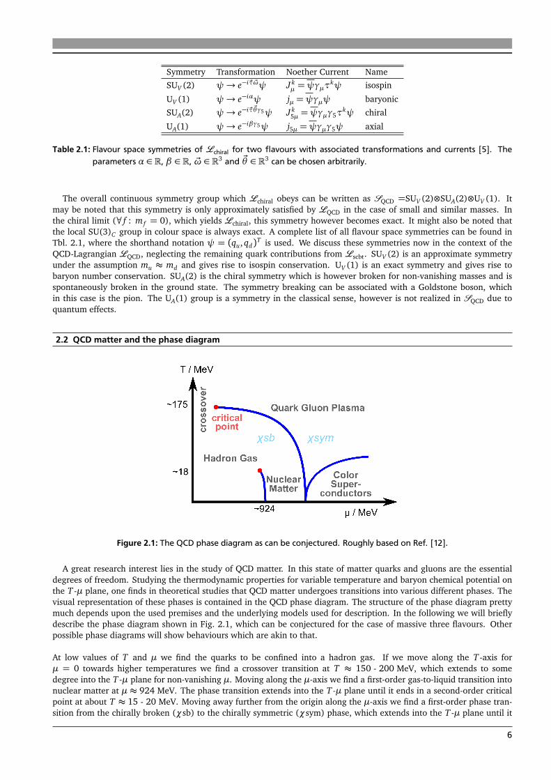
Figure 2.1: The QCD phase diagram as can be conjectured. Roughly based on Ref. [12].

A great research interest lies in the study of QCD matter. In this state of matter quarks and gluons are the essentialdegrees of freedom. Studying the thermodynamic properties for variable temperature and baryon chemical potential onthe T -µ plane, one finds in theoretical studies that QCD matter undergoes transitions into various different phases. Thevisual representation of these phases is contained in the QCD phase diagram. The structure of the phase diagram prettymuch depends upon the used premises and the underlying models used for description. In the following we will brieflydescribe the phase diagram shown in Fig. 2.1, which can be conjectured for the case of massive three flavours. Otherpossible phase diagrams will show behaviours which are akin to that.

At low values of T and µ we find the quarks to be confined into a hadron gas. If we move along the T -axis forµ = 0 towards higher temperatures we find a crossover transition at T ≈ 150 - 200 MeV, which extends to somedegree into the T -µ plane for non-vanishing µ. Moving along the µ-axis we find a first-order gas-to-liquid transition intonuclear matter at µ ≈ 924 MeV. The phase transition extends into the T -µ plane until it ends in a second-order criticalpoint at about T ≈ 15 - 20 MeV. Moving away further from the origin along the µ-axis we find a first-order phase tran-sition from the chirally broken (χsb) to the chirally symmetric (χsym) phase, which extends into the T -µ plane until it

6

ends in a second-order critical point, which also is a boundary of the crossover region. For high temperatures the hadrongas makes a phase transition into a quark gluon plasma via the first-order or the crossover transition. For low T and largeµ one finds a phase transtition to a colour superconducting phase.

As previously stated the phase diagram described above is conjectured, thus some of the proposed properties mightbe falsified in future studies. A more extensive and speculative description of a phase diagram can be found in Ref. [12].Compiling a phase diagram heavily relies on the use of QCD-like theories. Although the lattice QCD approach correspondsto solving the QCD-Lagrangian numerically via Monte Carlo methods, such first principle calculations become unusablefor Re(µ) 6= 0 due to the fermion sign problem. For that reason several approaches are being made to circumvent thisproblem, ranging from extrapolations from imaginary chemical potential to various reweighting methods. One methodwhich will play a crucial role in this work is the Taylor expansion of observables in terms of µ/T . A brief discussion of thefermion sign problem and various methods can be found in Ref. [2] and [1]. However it must be noted that despite allefforts, lattice QCD calculations can only be extended to the vicinity of µ < T . Thus, as long as the fermion sign problemcannot be fully resolved, lattice QCD calculations are still rendered useless for a large chunk of the T -µ plane.

2.3 The NJL model

As previously stated one way to study QCD matter is to use field theories which have a similar behaviour to the QCD-Lagrangian. Such an approach is the Nambu-Jona-Lasinio model. The Nambu-Jona-Lasinio model was originally pro-posed in a paper published in 1961 by Yoichiro Nambu and Giovanni Jona-Lasinio [3, 4]. Its original purpose was todescribe the mass of nucleons by a process of dynamic mass generation through self-energy contributions.

The whole description is an analogy to the BCS theory of superconductivity [13], in which phonons mediate an at-tractive force between pairs of electrons (Cooper pairs). To create excited electron states in the superconductor one isforced to break up the Cooper pairs first, thus there is an energy gap between the ground state and excited states inthe spectrum of superconductors. In the NJL model as originally proposed, the Cooper pairs have to be replaced withnucleons and anti-nucleons paired by an attractive force [3]. In this framework the nucleon masses are a consequence ofthis attractive interaction. Thus one speaks in the NJL model of a mass gap. Now in order to understand the QCD phasediagram, this model was later reinterpreted as a model of interacting quarks. In the same manner as before, attractiveinteractions now pair up quarks and anti-quarks. We additionally consider the quarks to possess a bare mass which wewill denote with m.

Basis for this reinterpretation of the NJL model is the underlying SNJL = SUV (2)⊗SUA(2)⊗UV (1) symmetry in thechiral NJL-Lagrangian, which is identical to the symmetry of the chiral QCD-Lagrangian contained in SQCD. The chiraland full Lagrangian of the NJL model are given by:

Lchiral =ψi /∂ψ+ GS[(ψψ)2 + (ψiγ5~τψ)

2],

LNJL =ψ(i /∂ −m)ψ+ GS[(ψψ)2 + (ψiγ5~τψ)

2].(2.4)

GS denotes the interaction strength of the scalar interaction terms. If we now compare the Lagrangian of the NJL model(2.4) to the one of QCD (2.1), we see that the basic difference lies in the fact that we replaced the parts incorporatingthe gluon fields with mathemically much easier to handle scalar interaction terms, which still display the important sym-metries. A direct consequence of these simplifications is that the SU(3)C group in colour space is now global. The chiralSUA(2) symmetry for m = 0 and its breaking is often coined as the most important feature of the NJL model, allowingone to investigate the chiral phase transition and its critical end point. The new interaction terms we incorporated canin fact be given a physical meaning via the Bethe-Salpeter equation. We can associate the first interaction term (ψψ)2

with a σ meson and the second term (ψiγ5τψ)2 with a π meson [5]. The NJL-Lagrangian as given by Eq. (2.4) canbe further extended by terms which obey the symmetry SNJL. In the following we will work with a Lagrangian which isfurther extended by a repulsive vector interaction term [14]:

LNJL ≡ψ(i /∂ −m)ψ+ GS[(ψψ)2 + (ψiγ5~τψ)

2]− GV (ψγµψ)2. (2.5)

The inclusion of this term is motivated by the Walecka model, in which additionally ω mesons play an important role.

The NJL model has two great shortcomings. One being that it does not feature confinement. The other is that sincethe interaction terms are constructed as contact interactions, the model is nonrenormalizable. The practical consequenceis that we need to define an energy scale on which the theory is valid. So in order to handle divergent momentum

7

integrals we must introduce a regularization scheme. Common regularization schemes are the three-momentum cutoff,the four-momentum cutoff, regularization in proper time and the Pauli-Villars method, with the latter three having theadvantage of being Lorentz-invariant. In this work we will focus on the use of a three-momentum cutoff. Details onthe other regularization schemes can be found in Ref. [5]. The three-momentum cutoff basically works by substitutingany divergent 3d momentum integrals over the spherical domain Sr with radius r ≡ ∞ with integrals over a sphericaldomain with finite radius r ≡ Λ.

In order to yield physically consistent results the cutoff parameter Λ is of course not chosen arbitrarily. Further, theinteraction strength GS and bare masses m f must also be determined in a way which yields physical meaningful results.This is usually done by fitting them to the pion mass mπ, the pion decay constant fπ (from π−→ µ−+νµ) and the quarkcondensates ⟨q f q f ⟩. In this work we will assume that mu = md ≡ m and use a parameter set determined in Ref. [14],with Λ = 587.9 MeV, GS = 2.44/Λ2 and m = 5.6 MeV. This set is tuned to reproduce a pion mass of mπ = 135 MeV, adecay constant of fπ = 92.4 MeV and quark condensate of ⟨ququ⟩= ⟨qdqd⟩= (−240.8 MeV)3.

8

3 Calculations

Based on our basic understanding of the NJL model from the previous chapter, we now want to derive and motivate theintroduction of the thermodynamic apparatus to describe QCD matter. In particular we are interested in calculating thegrand canonical potential Ω. As has been stated previously, a common technique to circumvent the fermion sign problemin lattice QCD is to expand thermodynamic functions and observables in terms of µ/T . Although the NJL model is acompletely different approach to describe QCD matter we will equivalently investigate an expansion in this model andcompare them to results obtained in lattice QCD. In particular we are interested into whether or not the vector couplingconstant GV can be tuned to deliver results which better resemble those of lattice QCD.

3.1 Pure scalar interaction in mean-field approximation

Figure 3.1: The Hartree approximation.

Although the bulk of this work will focus upon the inclusion of the vector interaction (GV 6= 0), there is a quitedemonstrative way of deriving the mass gap equation for a pure scalar interaction (GV = 0) in vacuum. In particular,incorporating the vector interaction would not change it. We can obtain the mentioned equation using the Hartreeapproximation (see Fig. 3.1), which expresses a relationship between the propagation of quarks with a dressed mass Mand quarks with a bare mass m, where the former is denoted by thick and the latter by thin lines. In terms of operatorsFig. 3.1 reads:

iS(p) = iS0(p) + iS0(p)(−iΣ)iS(p), (3.1)

where S(p) denotes the dressed, S0(p) the bare Feynman propagator andΣ the self-energy contribution. The propagatorsare simply fermionic propagators with their respective masses. The calculation of the self-energy part is non-trivial andneeds to be done explicitly for the given interaction terms. In the following we will just write down the necessarydefinitions and calculate Σ straightforwardly. For a more elaborate description of the necessary Feynman rules requiredfor the evaluation see Ref. [15]. The self-energy contribution can be calculated from the definition as follows:

Σ= 2iG jΓ j

∫

d4k

(2π)4Tr[Γ jS(k)]

= 2iGS1∫

d4k

(2π)4Tr[1S(k)] + 2iGS(iγ5τa)

∫

d4k

(2π)4Tr[iγ5τaS(k)]︸ ︷︷ ︸

=0

= 2iGS

∫

d4k

(2π)41

k2 −M2 + iεTr(γµkµ +M)

= 2iGS

∫

d4k

(2π)41

k2 −M2 + iεNcN f 4M =: 8GSNcN f M I(M),

(3.2)

where we have introduced the operators Γ j (i.e. Γσ = 1, Γ aπ = iγ5τa) and the coupling constants with G j (i.e. Gσ =

Gaπ = GS). We implicitly assumed that operators and traces have to be evaluated on the product Hilbert space. Using

these results we can now obtain the mass gap equation. Multiplying Eq. (3.1) by S−10 (p) = /p−m from the left side and

S−1(p) = /p−M from the right side yields:

S−10 (p) = S−1(p) +Σ

⇐⇒ /p−m= /p−M + 8GSNcN f M I(M)

⇐⇒ M = m+ 8GSNcN f M I(M).(3.3)

9

The equation obtained in the last step is the mass gap equation. In particular calculating dressed masses M relies onknowing the result of I(M). This expression can be easily evaluated in the vacuum case using the residue theorem.However in order to introduce temperatures T and chemical potential µ the I(M) function has to be modified using theMatsubara formalism. The calculation could be roughly sketched in a few steps for this particular integral, but the resultsone obtains are the same as when choosing a more generalized approach for GV 6= 0 and then setting GV a posteriori to0. Thus we instead postpone the results for GV = 0 to the latter sections of this work for a more comparative analysisand refer to [16] for an explicit treatment of the integral function I(M). The important lesson of this derivation becomesclearer in the next section. To make a long story short: We will see that the case of pure scalar interaction in Hartreeapproximation is equivalent to the introduction of the chiral quark condensate ⟨ψψ⟩.

3.2 Deriving the thermodynamic potential

We now want to calculate the thermodynamic potential Ω. We start by the definition of the thermodynamic potential Ωand the partition function Z:

Ω(T,µ) = −T

Vln[Z(T,µ)],

Z(T,µ) = Tr[e−1T (H−µN)].

(3.4)

It has to be noted that the Hamilton function is given by H =∫

d3 xH and the quark number by N =∫

d3 xψ†ψ. Inthis sense we calculate the HamiltonianH by taking the Legendre transform of the LagrangianL . We further introducethe condensates σ and ω:

σ = ⟨ψψ⟩,

ω= ⟨ψγ0ψ⟩.(3.5)

We further assume that we can approximate the interaction terms using their associated condensates, which yield ψψ=σ + δ(ψψ) and ψγ0ψ = ω + ε(ψψ). We linearize the squares of the interaction terms by considering the quadraticorders of δ and ε as negligible. Thus we get:

(ψψ)2 ≈ 2σ(ψψ)−σ2 and

(ψγ0ψ)2 ≈ 2ω(ψγ0ψ)−ω2.(3.6)

Having introduced two condensates for two interaction terms, we assume that the remaining terms do not result incondensates, thus are to be neglected [14]. This allows us to approximate the Lagrangian (2.5):

LNJ L +µ(ψγ0ψ)≈ψ(i /∂ − (m− 2GSσ)

︸ ︷︷ ︸

=:M

)ψ−σ2GS +ω2GV + (µ− 2GVω)

︸ ︷︷ ︸

=:µ

ψγ0ψ

=ψ(i /∂ −M)ψ−(M −m)2

4GS+(µ− µ)2

4GV+ µψ†ψ=:L +µψ†ψ.

(3.7)

We have introduced the dressed quark mass M and the renormalized chemical potential µ via gap equations:

M = m− 2GSσ,

µ= µ− 2GVω.(3.8)

In particular getting solutions for M and µ requires one to calculate σ and ω first (which are again functions of M andµ) and then to solve the gap equations self-consistently. The condensates can be calculated straightforwardly from thedefinition of the thermal expectation values and subsequent application of the Matsubara formalism or as a consequenceby enforcing thermodynamic consistency. We will choose the latter approach, however set aside an explicit discussion forthe next section. Taking the Legendre transform, we obtain:

H = ψ( j)π( j) −L = −ψ(iγk∂k −M)ψ+(M −m)2

4GS−(µ− µ)2

4GV− (µ−µ)ψ†ψ, (3.9)

10

with j denoting the components of the Dirac spinor, π the field momentum and k the spatial components. Putting theresult into Eq. (3.4), we see that Ω decomposes into a non-trivial and a trivial part:

Ω(T,µ; M , µ) = −T

VlnTr[exp

−1

T

∫

d3 x −ψ(iγk∂k −M)ψ− µψ†ψ

]︸ ︷︷ ︸

non-trivial

+(M −m)2

4GS−(µ− µ)2

4GV︸ ︷︷ ︸

trivial

. (3.10)

Note: M and µ are no independent variables but functions of µ and T . Thus we seperated them in the function header.Let us take a further look and identify some of the terms in the non-trivial part which we will denote with ΩM :

ΩM (T,µ; M , µ) = −T

VlnTr[exp

−1

T

∫

d3 x −ψ(iγk∂k −M)ψ︸ ︷︷ ︸

Hfree

−µ ψ†ψ︸︷︷︸

N

]= −T

Vln(Zfree). (3.11)

The argument of the potential is resembling to a free Fermi gas with mass M and chemical potential µ. An explicitcalculation of that expression is possible but lengthy and is given in Ref. [17] for a flavour- and colourless gas (Nc= N f=1)of fermions and anti-fermions. In the following we will just give the final result of ln(Zfree) and explain the physicalmeaning of the terms.

ln(Zfree) = 2NcN f︸ ︷︷ ︸

spins, coloursand flavours

V

∫

d3p

(2π)3

Ep

T︸︷︷︸

zero-pointenergy

+ ln[1+ exp

−1

T(Ep − µ)

]︸ ︷︷ ︸

quark contribution

+ ln[1+ exp

−1

T(Ep + µ)

]︸ ︷︷ ︸

anti-quark contribution

. (3.12)

The prefactor 2NcN f is the result of up and down spins, as well as the colours and flavours. The integral over thezero-point energy term Ep/T is divergent and needs to be treated by a regularization scheme of choice (in our casethe three-momentum cutoff). The remaining terms are contributions from quarks and anti-quarks. For the sake ofcompleteness we will now write down the final result for the thermodynamic potential Ω:

Ω(T,µ; M , µ) =(M −m)2

4GS−(µ− µ)2

4GV

− 2NcN f

¨

∫

SΛ

d3p

(2π)3Ep +

∫

R3

d3p

(2π)3

T ln(1+ e−1T (Ep−µ)) + T ln(1+ e−

1T (Ep+µ))

«

.

(3.13)

3.3 Self-consistency equations

As previously stated the equations (3.8) define us a set of gap equations which needs to be self-consistently solved. As afirst step one needs to calculate explicit expressions for the condensates σ = σ(T,µ; M , µ) and ω = ω(T,µ; M , µ). Fora thermodynamic consistent treatment we require that [14]:

dΩ

dm!=∂Ω

∂m= σ and −

dΩ

dµ!=−

∂Ω

∂ µ=ω. (3.14)

Calculating the total derivatives, we find that the partial derivatives ∂MΩ and ∂µΩ have to vanish in order to meetthe previously mentioned requirements. This leads to a set of equations which gives us explicit expressions for thecondensates σ and ω:

0=∂Ω

∂M=

M −m

2GS− 2N f Nc

∫

d3p

(2π)3M

Ep[1− np(T, µ)− np(T, µ)] =

M −m

2GS+σ,

0=∂Ω

∂ µ=µ− µ2GV

− 2N f Nc

∫

d3p

(2π)3[np(T, µ)− np(T, µ)] =

µ− µ2GV

−ω.

(3.15)

We have introduced the quark occupation number

np(T, µ) =1

1+ exp[−1/T (Ep − µ)](3.16)

and anti-quark occupation number np(T, µ) = np(T,−µ). One can interpret the equations (3.15) in terms of vectorcalculus: Arbitrary points (M , µ) at a preset temperature T and chemical potential µ are only solutions if they formextrema of Ω. A problem which becomes evident is that the map (T,µ) → (M , µ) is not necessarily injective, thus wemay find more than one solution for a given point (T,µ). Since in thermodynamics the potential Ω is supossed to beminimized, we will assume that the physically valid solution (M , µ) is the one which minimizes Ω the most. The solutionof the equation for µ is always unique for a given point (T,µ, M). At constant T and µ this allows us to introduce theparameterization µ = µ(M) and Ω(M) = Ω(M , µ(M)). So finding the physically legitimate solution (M , µ(M)) nowonly corresponds to finding the global minimum of Ω(M).

11

3.4 Extrema of the thermodynamic potential

-600 -400 -200 0 200 400 600-50

0

50

100

M MeV

W

Me

Vfm

-3

-600 -400 -200 0 200 400 600-20

-15

-10

-5

0

5

10

M MeVW

M

eV

fm-

3-600 -400 -200 0 200 400 600

-100

-50

0

50

100

150

M MeV

W

Me

Vfm

-3

Figure 3.2: Plots of the thermodynamic potential Ω(M) for different constant µ.Left image: GV = 0, m= 0; µ= 0, 300,368.6 and 400 MeV (red, green, blue, magenta).Middle image: GV = GS , m= 0; µ= 0,430, 440 and 444.3 MeV (red, green, blue, magenta).Right image: GV = 0, m= 5.6 MeV; µ= 0,375, 400 and 440 MeV (red, green, blue, magenta).

In this section we will discuss the influence of the bare mass m and the vector coupling constant GV on the extremaof Ω(M), which we know from the previous section are essential for knowing the legitimate solutions (M , µ(M)) for agiven point (T,µ). In this section we set T = 1 MeV and investigate the behaviour ofΩ(µ; M , µ(µ, M)) on the µ-M plane.

In Fig. 3.2 are three plots of the thermodynamic potential in the range from µ = 0 to 444.3 MeV. The specific val-ues for µ used in the plots were chosen to make characteristic behaviour evident, thus the plots are not directlycomparable. In the first and the second plot the bare mass m is kept constant at m = 0 (chiral limit) and the cou-pling constant GV is varied from 0 (first plot) to GS (second plot). The thermodynamic potential Ω remains symmetric,which is an obvious behaviour when considering the mass gap equation under the sign transformation M → −M inthe chiral limit. The characteristic features however change significantly. Although we observe a characteristic µ forGV = 0 at which the mass gap equation has five numerical solutions, we find that such a value of µ does not exist forGV = GS , at which the mass gap equation yields at maximum only three numerical solutions. An interesting feature isthat although one can easily verify that the mass gap equation always yields the trivial solution M = 0 in the chiral limit,this solution is not the physically relevant one for too low values of µ, even forming a maximum for low enough values.Another consequence of the symmetry is that for low values of µ one observes two identical solutions |M | with differentalgebraic sign. These can however not be distinguished by the minimization criteria. We therefore will just assume thatthe physical mass can only be positive.

Abandoning the discussion of the influence of the coupling constant GV , we now investigate the influence of thebare mass m on the thermodynamic potential. In the first and the third plot of Fig. 3.2 the coupling constant GV iskept constant at GV = 0 and we vary the bare mass m from m = 0 (first plot) to 5.6 MeV (third plot). While one cansee that Ω keeps its general shape, one can also see that the plot is skewed compared to the chiral limit. The mainconsequence of this is that the trivial solution M = 0 disappears and is replaced by solutions of M ¦ 0. The general trendwhich can be observed in all plots, is that for large µ there is only one numerical solution which either is M = 0 (chirallimit) or m ¦ M . This behaviour is somewhat intuitive when considering that our model reflects the chiral phase tran-sition in the QCD phase diagram and therefore tries to replicate the bare quark mass m. Deviations from this expectedbehaviour can be dependent on the used regularization scheme.

3.5 Solutions of the self-consistency equations for variable chemical potential

In pursuit of automating the sketched way of solving M for variable µ in the previous section (we keep the temperatureat T = 1 MeV), we can construct an algorithm which is capable of providing a function M(µ). The resulting plots forvariable coupling constant GV and bare mass m are listed in the upper row of Fig. 3.3.We can observe that the generated dynamical mass M is discontinuous in µ for GV = 0 and 0.5 GS , whereas it is con-tinuous for GV = GS . The discontinuous behaviour is already evident when comparing the parametric plots of the

12

300 350 400 450 500

0

100

200

300

400

500

Μ MeV

M

Me

V

300 350 400 450 500

0

100

200

300

400

500

Μ MeV

M

Me

V

300 350 400 450 500

0

100

200

300

400

500

Μ MeV

M

Me

V

300 350 400 450 500300

350

400

450

500

Μ MeV

Μ

Me

V

300 350 400 450 500

300

350

400

450

Μ MeV

Μ

Me

V

300 350 400 450 500

300

350

400

450

Μ MeV

Μ

Me

V

Figure 3.3: Plots of M(µ) (upper row) and µ (lower row) for variable bare quark mass m and vector coupling constantGV . From left to right: GV = 0, 0.5 GS and GS . The blue lines correspond to m= 5.6 MeV and the red lines tom= 0.

thermodynamic potential in Fig. 3.2. The plots in Fig. 3.3 can already be used to classify phase transitions. The dis-continuous behaviours of the mass plots for GV = 0 and GV = 0.5 GS are classified as first order phase transitions. Inparticulary they correspond to the chiral phase transition at T = 1 MeV in the phase diagram in Fig. 2.1. The phasetransition for GV = GS and m = 0 is continuous, however it is discontinuous in its derivative with respect to µ. This isclassified as second order phase transition. The case of GV = GS and m = 5.6 MeV is continuous in all of its derivativeswith respect to µ. It is commonly labeled as a crossover transition, however, in fact it is not a phase transition.

Since we now have a function M(µ) we can also calculate solutions µ(µ) = µ(µ, M(µ)). The resulting plots aregiven in the lower row of Fig. 3.3. The GV = 0 case is obvious since the second gap equation yields µ = µ, thecourse of the remaining plots for GV = 0.5 and GS is a direct consequence of the behaviour of M(µ), thus will not befurther discussed.

3.6 Calculation of the Taylor coefficients to sixth order

We now want to calculate the Taylor coefficients of the thermodynamic potentialΩ(T,µ) in terms of µ/T at the expansionpoint µ/T = 0 to sixth order. We therefore just expand Ω in terms of µ/T :

Ω(T,µ) =∞∑

n=0

c∗n

µ

T

n=∞∑

n=0

1

n!

∂ nΩ

∂ (µ/T )n

µ/T=0

µ

T

n. (3.17)

Further we will follow the convention of using the reduced thermodynamic potential Ω = −Ω/T 4, thus effectivelymultiplying the definition of the coefficient by a prefactor:

cn = −1

T 4 c∗n = −T n−4 1

n!

∂ nΩ

∂ µn

µ=0

. (3.18)

13

We can calculate the Taylor coefficients from the definition (3.18) straightforwardly. However, we only have to calculatethe Taylor coefficients of even order. This property is realized due to the symmetry of Ω under charge conjugation, whichis a fundamental property of QCD. In a world in which we replace quarks by anti-quarks and vice versa the physics shouldstay the same. We can further prove that this property is fulfilled using the gap equations (3.15).

Using the gap equation of the renormalized chemical potential µ and the fact that solutions of this equation are uniquefor a given point (T,µ, M), we find under the transformation µ→−µ, that −µ(−µ) = µ(µ), thus rendering the solutionsanti-symmetric in µ. Further taking a look at the mass gap equation shows that M(µ(µ)) = M(−µ(µ)) = M(µ(−µ)),thus rendering the solutions symmetric in µ. So in conclusion we find that (µ, M)

µ→−µ−−−→ (−µ, M). It is now quite obvious

when applying the transformation to Eq. (3.13) that Ω is symmetric in µ. In particular we can now easily prove that oddterms have to vanish in the Taylor expansion:

Ω(T,µ) =∞∑

n even

c∗n

µ

T

n+

∞∑

n odd

c∗n

µ

T

n !=

∞∑

n even

c∗n

µ

T

n+

∞∑

n odd

−c∗n

µ

T

n= Ω(T,−µ). (3.19)

Thus Eq. (3.19) is only satisfied for non-vanishing values µ/T , if odd ordered coefficients vanish .

So we now only have to calculate the Taylor coefficients of second, fourth and sixth order. For that purpose we willuse the finite difference method and approximate the derivatives with central difference quotients. In particular we use:

∂ 2Ω

∂ µ2

µ=0

≈1

12∆2

§

2[−Ω(2∆) + 16Ω(∆)]− 30Ω(0)ª

,

∂ 4Ω

∂ µ4

µ=0

≈1

6∆4

§

2[−Ω(3∆) + 12Ω(2∆)− 39Ω(∆)] + 56Ω(0)ª

and

∂ 6Ω

∂ µ6

µ=0

≈1

240∆6

§

2[13Ω(5∆)− 190Ω(4∆) + 1305Ω(3∆)− 4608Ω(2∆) + 9690Ω(∆)]− 12276Ω(0)ª

.

(3.20)

The expressions were shortened using the symmetry of Ω in respect to µ= 0. The order of approximation was chosenso that approximation errors are of third power in ∆ for the second and fourth derivative and of fifth power for the sixthderivative. This directly corresponds to using five, seven and eleven sampling points for the derivatives. Further the gridspacing was chosen for every coefficient so that numerical errors which become emergent for large values of T and toosmall grid spacing are minimized.

When discussing the course of the Taylor coefficients in the high temperature district, it is useful to refer to the lim-its of the Stefan-Boltzmann gas. The Stefan-Boltzmann gas with thermodynamic potential ΩSB, corresponds to thepotential of a free quark gluon gas:

−ΩSB

T 4 = 2NcN f

7π2

360+

1

12

µ

T

2+

1

24π2

µ

T

4

−Ωglue

T 4 , (3.21)

where Ωglue is the gluonic contribution with Ωglue ∝ T 4. The Stefan-Boltzmann limits of the coefficients can now bestraightforwardly calculated by taking the derivatives of ΩSB and the limit µ/T → 0 . In particular we find in this limit:c2 = 1, c4 = 0.051 and c6 = 0.

A presentation of all calculated Taylor coefficients for m = 5.6 MeV, variable order n and vector coupling constantGV is given in Fig. 3.4. All calculations were performed in C++ using some functions contained in the GNU ScientificLibrary. Roughly, one can say that coefficients of second and fourth order are always positive, have one maximum orbecome asymptotical constant for GV = 0 and large T , while sixth order coefficients always become asymptotical zero,but also possess a zero crossing, a positive maximum and a negative minimum. Much more information yields the com-parison for constant order n and variable coupling constant GV , which we can see in the fourth lower row in Fig. 3.4.The second order coefficient at GV = 0 is a steeply rising function reaching a plateau value of c2 ≈ 1 for large T . Puttingin a vector interaction destroys the constant Stefan-Boltzmann limit and creates a global positive maximum at aboutT ≈ 200 MeV, which becomes smaller the greater GV gets. The fourth order coefficient is also a steeply rising function,reaching a global maximum at about T ≈ 190 MeV and then sinking to reach its Stefan-Boltzmann limit for large Tof about c4 ≈ 0.051. Turning on the vector interaction also destroys the Stefan-Boltzmann limit and results into themaximum shrinking the greater GV gets. The sixth order coefficient rises first to a positive maximum, then does a zerocrossing, reaches a minimum and approaches then 0 for large T . Turning on the vector interaction drastically reducesthe magnitudes of the extrema.

14

0 100 200 300 4000.0

0.2

0.4

0.6

0.8

1.0

T MeV

c2

1

0 100 200 300 4000.00

0.05

0.10

0.15

0.20

T MeV

c4

1

0 100 200 300 400

-0.10

-0.08

-0.06

-0.04

-0.02

0.00

0.02

0.04

T MeV

c6

1

0 100 200 300 4000.0

0.1

0.2

0.3

0.4

0.5

0.6

0.7

T MeV

c2

1

0 100 200 300 4000.00

0.01

0.02

0.03

0.04

0.05

T MeV

c4

1

0 100 200 300 400-0.012

-0.010

-0.008

-0.006

-0.004

-0.002

0.000

0.002

T MeV

c6

1

0 100 200 300 4000.0

0.1

0.2

0.3

0.4

0.5

T MeV

c2

1

0 100 200 300 4000.000

0.005

0.010

0.015

0.020

0.025

T MeV

c4

1

0 100 200 300 400

-0.0025

-0.0020

-0.0015

-0.0010

-0.0005

0.0000

0.0005

T MeV

c6

1

0 100 200 300 4000.0

0.2

0.4

0.6

0.8

1.0

T MeV

c2

1

0 100 200 300 4000.00

0.05

0.10

0.15

0.20

T MeV

c4

1

0 100 200 300 400

-0.10

-0.08

-0.06

-0.04

-0.02

0.00

0.02

0.04

T MeV

c6

1

Figure 3.4: Taylor coefficients of variable order n and vector coupling constant GV .From left to right: Taylor coefficients of order 2, 4 and 6.First three rows from top to bottom: Taylor coefficients for GV = 0, 0.5 GS and GS .Fourth row on the bottom: Comparative plots the Taylor coefficients for coupling constant GV = 0, 0.5 GSand GS (blue, red, green).

15

3.7 Comparison to lattice data

ã

ã

ã

ã

ã

ã

ã

ã

ãã

ã

100 150 200 250 300 350 4000.0

0.2

0.4

0.6

0.8

1.0

T MeV

c2

1

ã

ã

ã

ãã

ã

ã

ã

ã

ãã

100 150 200 250 300 350 4000.0

0.1

0.2

0.3

0.4

0.5

T MeV

c4

1

100 150 200 250 300 350 400

-0.10

-0.05

0.00

0.05

T MeV

c6

1

Figure 3.5: Comparison of Taylor coefficients c2, c4 and c6 (left to right) obtained from lattice QCD calculations (red andgreen) to the vector interaction extended NJL model (black). Red squares represent data by C.R. Allton et al.[6] and green squares M. Cheng et al. [7]. Empty green squares were done on a 163 × 4 lattice, filled greensquares on a 243 × 6 lattice. The vector coupling strength is set in the extended NJL model to GV = 0, 0.5 GSand GS (continuous, dashed, dotted).

In this section we now want to compare the results we have obtained to available lattice data and find out whether ornot we can tune the vector coupling constant GV to deliver better results with the vector interaction extended NJL model.In particular we will use results of calculations done by C.R. Allton et al. [6] (red data) for two flavours on a 163 × 4lattice using p4-improved staggered fermions with bare quark mass m/T = 0.4 and M. Cheng et al. [7] (green data) forthree flavours on a 163×4 and a 243×6 lattice using p4-improved staggered fermions and fixed quark masses. The datacan be directly found in Ref. [6] and [7], errors were taken from the plots. The temperature values which were used forthe calculated sampling points are all given in respect to the pseudocritical temperature T0, which is the temperature atwhich the crossover transition for µ = 0 is located. This allows us to translate the results into the NJL model, in whichthe pseudocritical temperature is estimated to be T0 = 193.6 MeV [16].

Comparing the lattice data with the results in our extended NJL model (Fig. 3.5), we see that the course of the Tay-lor coefficients, as well as the Stefan-Boltzmann limits, are best replicated by the NJL model for GV = 0. Further onefinds a systematic discrepance between lattice data and the NJL model. For the lattice data of c2 and c4 one sees thatthe flank is significantly shifted to higher temperatures. For data provided by Ref. [6] (red) c2 does not reach the pre-dicted Stefan-Boltzmann limit, instead converges towards c2 ≈ 0.8. This does not comply with data provided by Ref.[7] (green), in which c2 does indeed reach its predicted limit. So this abberation might be a result due to the temper-ature dependent bare mass. The remaining coefficients c4 and c6 seem to follow the trend of converging towards theirpredicted limits. A notable feature of c4 in lattice calculations is that its peak is higher than in the NJL model. The dataprovided on c6 is highly speculative due to the large errors, however for that reason complies with the scalar NJL modelexcept for a few data points.

Overall the study confirms a similar analysis done by J. Steinheimer and S. Schramm in 2011 [18], comparing sec-ond and fourth order Taylor coefficients of the PNJL and QHC model with lattice QCD calculations from Ref. [7].

16

4 Résumé and outlook

The motivation of this work was to investigate the Taylor coefficients of the NJL model under the inclusion of a repulsivevector interaction term −GV (ψγµψ)2 and find out whether or not the vector coupling GV can be tuned to deliver betterresults in comparison to lattice QCD calculations. For the investigation the NJL model in the two flavour case under theinclusion of an up and down quark of equal mass and chiral condensate was chosen. Divergent momentum integrals areregularized using a sharp three-momentum cutoff, which however is not Lorentz invariant. The parameter set which isused was determined by Ref. [14].

Investigating first the case of a pure scalar interaction, which is the special case for GV = 0, actually shows that onecan derive the mass gap equation using the Hartree approximation. In particular this is equivalent to the introduction ofthe chiral quark condensate ⟨ψψ⟩. The Lagrangian with the vector interaction term can be treated by the introductionof the condensates ⟨ψψ⟩ and ⟨ψγ0ψ⟩. These condensates result into a set of two gap equations, one describing thegenerated mass M and the other the renormalized chemical potential µ. Approximating the interaction terms with theirassociated condensates allows us to calculate the thermodynamic potential Ω of the grand canonical ensemble. One canshow that pairs of M and µ are only valid solutions of the gap equations if they are extrema of Ω. If there is morethan one solution (M , µ) for a given point (T,µ), the one is chosen which is a global minimum of Ω. Following theseprinciples one can now construct an algorithm to calculate (M , µ) for any given point (T,µ) and thus Ω. Calculatingthe Taylor coefficients can now be done numerically using finite differences. Furthermore one just needs to calculateeven ordered coefficients. The odd orders vanish as a direct consequence of the symmetry of QCD under charge con-jugation (µ → −µ) and thus Ω. In general a non-vanishing vector interaction (GV 6= 0) leads to a reduction of themagnitude of the course of the coefficients. Further the Stefan-Boltzmann limits are destroyed for c2 and c4. Comparingthe coefficients to lattice data from Ref. [6] and [7] shows that there are some significant discrepancies, however thecourse of the lattice results, as well as the Stefan-Boltzmann limits, are best replicated by neglecting the vector interac-tion term. This conclusion complies with an analysis of Taylor coefficients done in Ref. [18] for the PNJL and QHC model.

Summing up the results one obtains from the study of these QCD-like theories shows that it seems to become evi-dent that vector interaction terms generally are negligible if one aims to get results which are similar to those of latticeQCD. Although this should hold up to various other lattice QCD extension methods apart from the Taylor expansion tech-nique, it is an interesting afterthought whether or not the effects are as drastical. An answer to this question thereforeremains open for future studies.

17

Bibliography

[1] M. P. Lombardo, “Lattice QCD at finite temperature and density,” Modern Physics Letters A, vol. 22, pp. 457–472,2005.

[2] C. Schmidt, “Lattice QCD at finite density,” PoS, vol. LAT2006, p. 021, 2006.

[3] Y. Nambu and G. Jona-Lasinio, “Dynamical model of elementary particles based on an analogy with superconduc-tivity. I,” Phys. Rev., vol. 122, pp. 345–358, 1961.

[4] Y. Nambu and G. Jona-Lasinio, “Dynamical model of elementary particles based on an analogy with superconduc-tivity. II,” Phys. Rev., vol. 124, pp. 246–254, 1961.

[5] S. P. Klevansky, “The Nambu-Jona-Lasinio model of quantum chromodynamics,” Review of Modern Physics, vol. 64,pp. 649–708, 1992.

[6] C. R. Allton et al., “Thermodynamics of Two Flavor QCD to Sixth Order in Quark Chemical Potential,” Phys. Rev. D,vol. 71, p. 054508, 2005.

[7] M. Cheng et al., “Baryon number, strangeness, and electric charge fluctuations in QCD at high temperature,” Phys.Rev. D, vol. 79, p. 074505, 2009.

[8] M. Ablikim et al., “Observation of a charged charmoniumlike structure in e+e− → π+π−J/ψ atp

s = 4.26 GeV,”Phys. Rev. Lett., vol. 110, p. 252001, 2013.

[9] Z. Q. Liu et al., “Study of e+e− → π+π−J/ψ and observation of a charged charmoniumlike state at Belle,” Phys.Rev. Lett., vol. 110, p. 252002, 2013.

[10] G. Ecker, “Quantum Chromodynamics,” arXiv:1205.1815, 2006.

[11] A. Grozin, “Quantum Chromodynamics,” arXiv:hep-ph/0604165, 2012.

[12] K. Fukushima and T. Hatsuda, “The phase diagram of dense QCD,” Rept. Prog. Phys., vol. 74, p. 014001, 2010.

[13] J. Bardeen, L. N. Cooper and J. R. Schrieffer, “Microscopic theory of superconductivity,” Phys. Rev., vol. 106,pp. 162–164, 1957.

[14] M. Buballa, “NJL-model analysis of dense quark matter,” Phys.Rept., vol. 407, pp. 205 – 376, 2004.

[15] S. Möller, “Pion-Pion scattering and shear viscosity in the Nambu-Jona-Lasinio model,” Master’s thesis, TU Darm-stadt, 2013.

[16] D. Scheffler, “NJL model study of the QCD phase diagram using the taylor expansion technique,” Bachelor’s thesis,TU Darmstadt, 2007.

[17] J. I. Kapusta and C. Gale, Finite-Temperature Field Theory. Cambridge University Press, 2006.

[18] J. Steinheimer and S. Schramm, “The problem of repulsive quark interactions - Lattice versus mean field models,”Phys. Lett. B, vol. 696, pp. 257 – 261, 2011.

18