arX

iv:1

207.

7207

v1 [

mat

h.PR

] 3

1 Ju

l 201

2

Normal Approximations for Wavelet Coefficients on

Spherical Poisson Fields

Claudio DurastantiDepartment of Mathematics, University of Rome Tor Vergata

Domenico Marinucci∗

Department of Mathematics, University of Rome Tor Vergata

Giovanni PeccatiUnite de Recherche en Mathematiques, Luxembourg University

November 2, 2018

Abstract

We compute explicit upper bounds on the distance between the law of a multivari-ate Gaussian distribution and the joint law of wavelets/needlets coefficients based ona homogeneous spherical Poisson field. In particular, we develop some results fromPeccati and Zheng (2011), based on Malliavin calculus and Stein’s methods, to assessthe rate of convergence to Gaussianity for a triangular array of needlet coefficientswith growing dimensions. Our results are motivated by astrophysical and cosmolog-ical applications, in particular related to the search for point sources in Cosmic Raysdata.

Keywords and Phrases: Berry-Esseen Bounds; Malliavin Calculus; Multidimen-sional Normal Approximation; Poisson Process; Stein’s Method; Spherical Wavelets.

AMS Classification: 60F05; 42C40; 33C55; 60G60; 62E20.

1 Introduction

The aim of this paper is to establish multidimensional normal approximation results forvectors of random variables having the form of wavelet coefficients integrated with respectto a Poisson measure on the unit sphere. The specificity of our analysis is that we requirethe dimension of such vectors to grow to infinity. Our techniques are based on recently

∗Corresponding author, email: marinucc@mat.uniroma2.it. Research supported by the ERC GrantPascal, n.277742

1

obtained bounds for the normal approximation of functionals of general Poisson measures(see [42, 43]), as well as on the use of the localization properties of wavelets systems onthe sphere (see [35], as well as the recent monograph [30]). A large part of the paper isdevoted to the explicit determination of the above quoted bounds in terms of dimension.

1.1 Motivation and overview

A classical problem in asymptotic statistics is the assessment of the speed of convergenceto Gaussianity (that is, the computation of explicit Berry-Esseen bounds) for parametricand nonparametric estimation procedures – for recent references connected to the maintopic of the present paper, see for instance [17, 29, 55]. In this area, an important noveldevelopment is given by the derivation of effective Berry-Esseen bounds by means of thecombination of two probabilistic techniques, namely the Malliavin calculus of variationsand the Stein’s method for probabilistic approximations. The monograph [8] is the standardmodern reference for Stein’s method, whereas [38] provides an exhaustive discussion of theuse of Malliavin calculus for proving normal approximation results on a Gaussian space.The fact that one can use Malliavin calculus to deduce normal approximation bounds (intotal variation) for functionals of Gaussian fields was first exploited in [37] – where onecan find several quantitative versions of the “fourth moment theorem” for chaotic randomvariables proved in [39]. Lower bounds can also be computed, entailing that the rates ofconvergence provided by these techniques are sharp in many instances – see again [38].

In a recent series of contributions, the interaction between Stein’s method and Malliavincalculus has been further exploited for dealing with the normal approximation of functionalsof a general Poisson random measure. The most general abstract results appear in [42] (forone-dimensional normal approximations) and [43] (for normal approximations in arbitrarydimensions). These findings have recently found a wide range of applications in the fieldof stochastic geometry – see [25, 26, 33, 27, 48] for a sample of geometric applications, aswell as the webpage

http://www.iecn.u-nancy.fr/∼nourdin/steinmalliavin.htm

for a constantly updated resource on the subject.

The purpose of this paper is to apply and extend the main findings of [42, 43] in order tostudy the multidimensional normal approximation of the elements of the first Wiener chaosof a given Poisson measure. Our main goal is to deduce bounds that are well-adapted todeal with applications where the dimension of a given statistic increases with the number ofobservations. This is a framework which arises naturally in many relevant fields of modernstatistical analysis; in particular, our principal motivation originates from the implemen-tation of wavelet systems on the sphere. In these circumstances, when more and more databecome available, a higher number of wavelet coefficients is evaluated, as it is customarilythe case when considering, for instance, thresholding nonparametric estimators. We shall

2

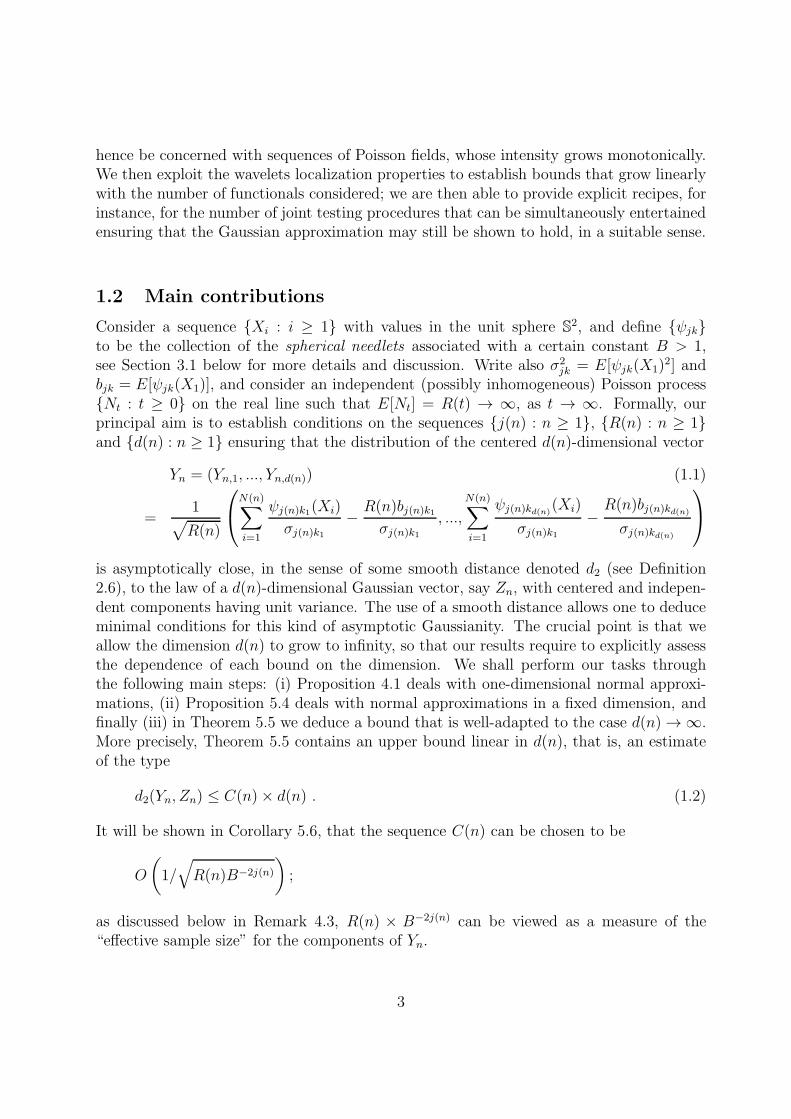
hence be concerned with sequences of Poisson fields, whose intensity grows monotonically.We then exploit the wavelets localization properties to establish bounds that grow linearlywith the number of functionals considered; we are then able to provide explicit recipes, forinstance, for the number of joint testing procedures that can be simultaneously entertainedensuring that the Gaussian approximation may still be shown to hold, in a suitable sense.

1.2 Main contributions

Consider a sequence Xi : i ≥ 1 with values in the unit sphere S2, and define ψjk

to be the collection of the spherical needlets associated with a certain constant B > 1,see Section 3.1 below for more details and discussion. Write also σ2

jk = E[ψjk(X1)2] and

bjk = E[ψjk(X1)], and consider an independent (possibly inhomogeneous) Poisson processNt : t ≥ 0 on the real line such that E[Nt] = R(t) → ∞, as t → ∞. Formally, ourprincipal aim is to establish conditions on the sequences j(n) : n ≥ 1, R(n) : n ≥ 1and d(n) : n ≥ 1 ensuring that the distribution of the centered d(n)-dimensional vector

Yn = (Yn,1, ..., Yn,d(n)) (1.1)

=1√R(n)

N(n)∑

i=1

ψj(n)k1(Xi)

σj(n)k1− R(n)bj(n)k1

σj(n)k1, ...,

N(n)∑

i=1

ψj(n)kd(n)(Xi)

σj(n)k1−R(n)bj(n)kd(n)

σj(n)kd(n)

is asymptotically close, in the sense of some smooth distance denoted d2 (see Definition2.6), to the law of a d(n)-dimensional Gaussian vector, say Zn, with centered and indepen-dent components having unit variance. The use of a smooth distance allows one to deduceminimal conditions for this kind of asymptotic Gaussianity. The crucial point is that weallow the dimension d(n) to grow to infinity, so that our results require to explicitly assessthe dependence of each bound on the dimension. We shall perform our tasks throughthe following main steps: (i) Proposition 4.1 deals with one-dimensional normal approxi-mations, (ii) Proposition 5.4 deals with normal approximations in a fixed dimension, andfinally (iii) in Theorem 5.5 we deduce a bound that is well-adapted to the case d(n) → ∞.More precisely, Theorem 5.5 contains an upper bound linear in d(n), that is, an estimateof the type

d2(Yn, Zn) ≤ C(n)× d(n) . (1.2)

It will be shown in Corollary 5.6, that the sequence C(n) can be chosen to be

O

(1/√R(n)B−2j(n)

);

as discussed below in Remark 4.3, R(n) × B−2j(n) can be viewed as a measure of the“effective sample size” for the components of Yn.

3

1.3 About de-Poissonization

Our results can be used in order to deduce the asymptotic normality of de-Poissonizedlinear statistics with growing dimension. To illustrate this point, assume that the randomvariables Xi are uniformly distributed on the sphere. Then, it is well known that bjk = 0,whenever j > 1. In this framework, when j(n) > 1 for every n, R(n) = n and d(n)/n1/4 →0, the conditions implying that Yn is asymptotically close to Gaussian, automatically ensurethat the law of the de-Poissonized vector

Y ′n = (Y ′

n,1, ..., Y′n,d(n)) =

1√n

(n∑

k=1

ψj(n)k1(Xi)

σj(n)k1, ...,

n∑

k=1

ψj(n)kd(n)(Xi)

σj(n)kd(n)

)(1.3)

is also asymptotically close to Gaussian. The reason for this phenomenon is nested in thestatement of the forthcoming (elementary) Lemma 1.1.

Lemma 1.1 Assume that R(n) = n, that the Xi’s are uniformly distributed on the sphere,and that j(n) > 1 for every n. Then, there exists a universal constant M such that, forevery n and every Lipschitz function ϕ : Rd(n) → R, the following estimate holds:

∣∣∣E[ϕ(Y ′n)]−E[ϕ(Yn)]

∣∣∣ ≤M‖ϕ‖Lipd(n)

n1/4.

Proof. Fix l = 1, ..., d(n), and write βl(x) =ψj(n)kl

(x)

σj(n)kl

, in such a way that E[βl(X1)2] =

1. One has that

E[(Y ′n,l − Yn,l)

2] = 2(1− αn),

where

αn =1

n

n∑

m=0

e−nnm

m!(n ∧m) = 1− e−nnn

n!.

This gives the estimate

E[|Y ′n,l − Yn,l|] ≤

√E[(Y ′

n,l − Yn,l)2] ≤√

2e−nnn

n!,

so that the conclusion follows from an application of Stirling’s formula and of the Lipschitzproperty of ϕ.

Remark 1.2 (i) Lemma 1.1 implies that one can obtain an inequality similar to (1.2)for Y ′

n, that is:

d2(Y′n, Zn) ≤

(C(n) +

M

n1/4

)× d(n).

4

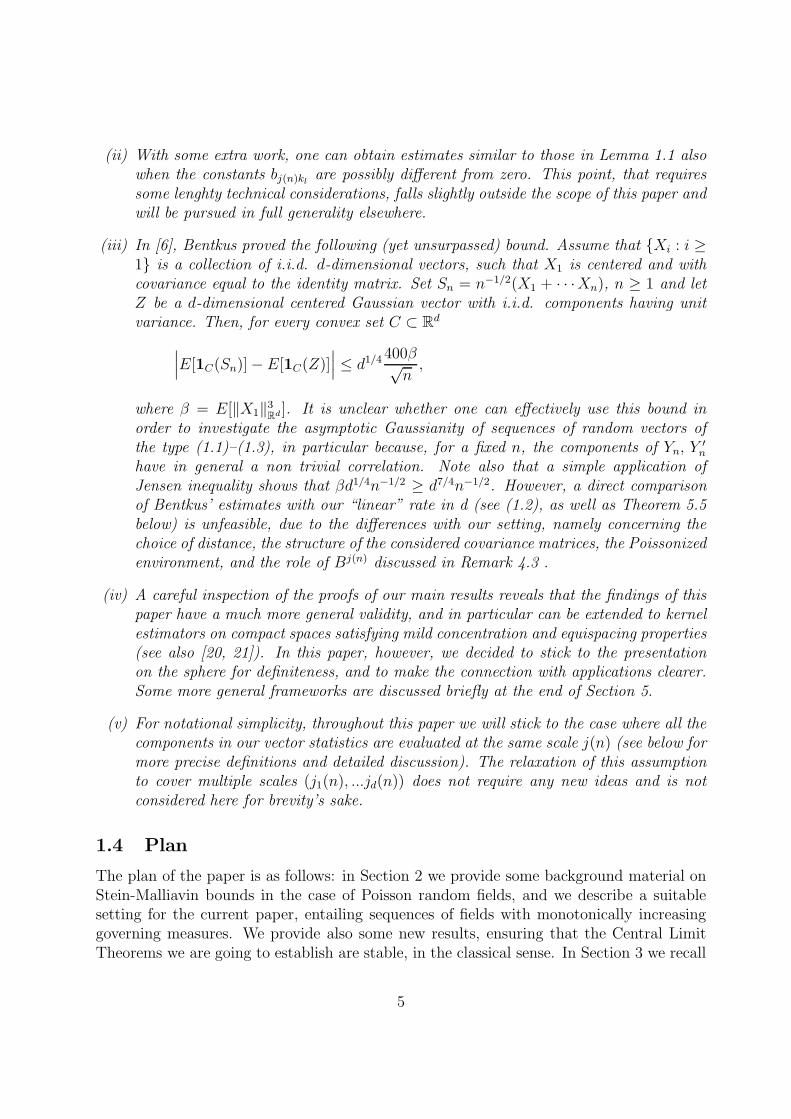
(ii) With some extra work, one can obtain estimates similar to those in Lemma 1.1 alsowhen the constants bj(n)kl are possibly different from zero. This point, that requiressome lenghty technical considerations, falls slightly outside the scope of this paper andwill be pursued in full generality elsewhere.

(iii) In [6], Bentkus proved the following (yet unsurpassed) bound. Assume that Xi : i ≥1 is a collection of i.i.d. d-dimensional vectors, such that X1 is centered and withcovariance equal to the identity matrix. Set Sn = n−1/2(X1 + · · ·Xn), n ≥ 1 and letZ be a d-dimensional centered Gaussian vector with i.i.d. components having unitvariance. Then, for every convex set C ⊂ R

d

∣∣∣E[1C(Sn)]− E[1C(Z)]∣∣∣ ≤ d1/4

400β√n,

where β = E[‖X1‖3Rd]. It is unclear whether one can effectively use this bound inorder to investigate the asymptotic Gaussianity of sequences of random vectors ofthe type (1.1)–(1.3), in particular because, for a fixed n, the components of Yn, Y

′n

have in general a non trivial correlation. Note also that a simple application ofJensen inequality shows that βd1/4n−1/2 ≥ d7/4n−1/2. However, a direct comparisonof Bentkus’ estimates with our “linear” rate in d (see (1.2), as well as Theorem 5.5below) is unfeasible, due to the differences with our setting, namely concerning thechoice of distance, the structure of the considered covariance matrices, the Poissonizedenvironment, and the role of Bj(n) discussed in Remark 4.3 .

(iv) A careful inspection of the proofs of our main results reveals that the findings of thispaper have a much more general validity, and in particular can be extended to kernelestimators on compact spaces satisfying mild concentration and equispacing properties(see also [20, 21]). In this paper, however, we decided to stick to the presentationon the sphere for definiteness, and to make the connection with applications clearer.Some more general frameworks are discussed briefly at the end of Section 5.

(v) For notational simplicity, throughout this paper we will stick to the case where all thecomponents in our vector statistics are evaluated at the same scale j(n) (see below formore precise definitions and detailed discussion). The relaxation of this assumptionto cover multiple scales (j1(n), ...jd(n)) does not require any new ideas and is notconsidered here for brevity’s sake.

1.4 Plan

The plan of the paper is as follows: in Section 2 we provide some background material onStein-Malliavin bounds in the case of Poisson random fields, and we describe a suitablesetting for the current paper, entailing sequences of fields with monotonically increasinggoverning measures. We provide also some new results, ensuring that the Central LimitTheorems we are going to establish are stable, in the classical sense. In Section 3 we recall

5

some background material on the construction of tight wavelet systems on the sphere (see[35, 36] for the original references, as well as [30, Chapter 10]) and we explain how to expressthe corresponding wavelet coefficients in terms of stochastic integrals with respect to aPoisson random measure. We also illustrate shortly some possible statistical applications.In Section 4 we provide our bounds in the one-dimensional case; these are simple resultswhich could have been established by many alternative techniques, but still they providesome interesting insights into the “effective area of influence” of a single component of thewavelet system. The core of the paper is in Section 5, where the bound is provided in themultidimensional case, allowing in particular for the number of coefficients to be evaluatedto grow with the number of observations. This result requires a careful evaluation of theupper bound, which is made possible by the localization properties in real space of thewavelet construction.

2 Poisson Random Measures and Stein-Malliavin

Bounds

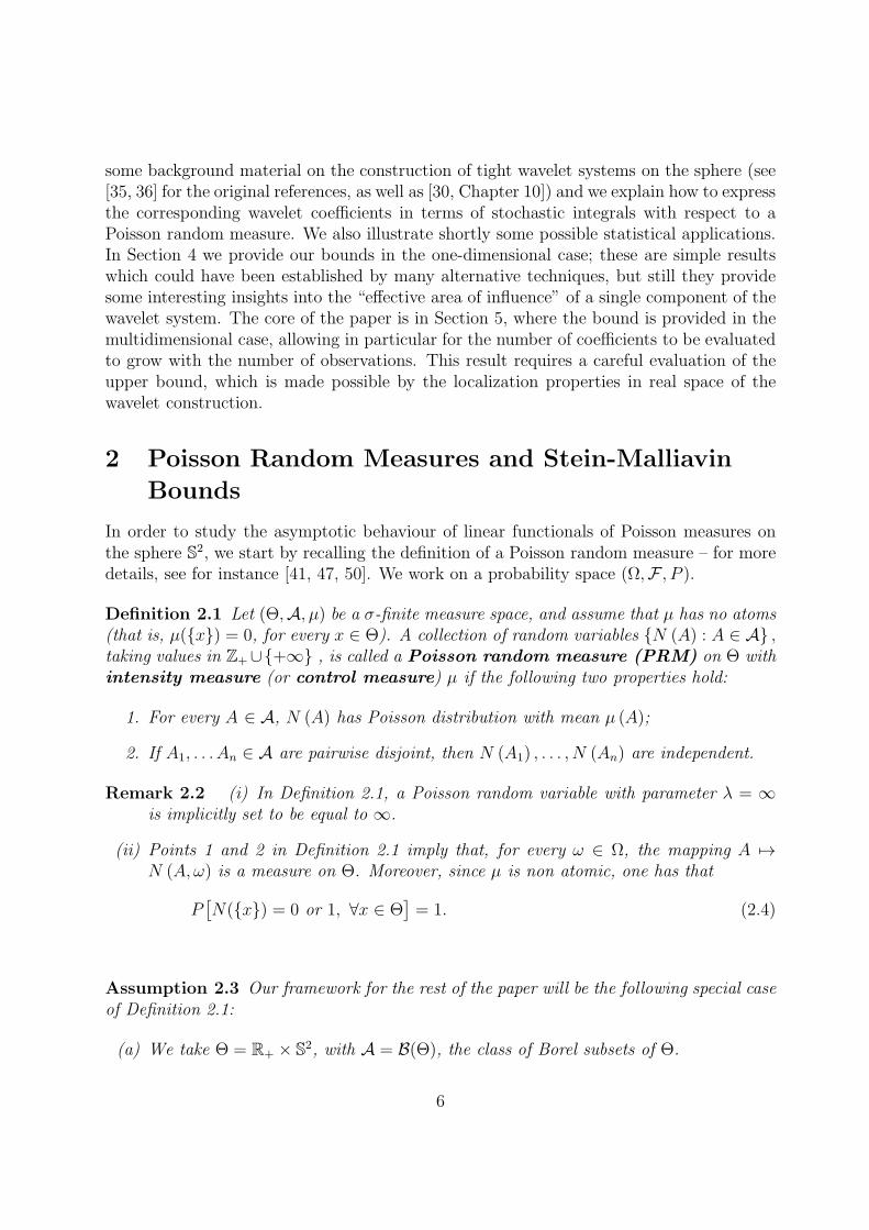
In order to study the asymptotic behaviour of linear functionals of Poisson measures onthe sphere S

2, we start by recalling the definition of a Poisson random measure – for moredetails, see for instance [41, 47, 50]. We work on a probability space (Ω,F , P ).

Definition 2.1 Let (Θ,A, µ) be a σ-finite measure space, and assume that µ has no atoms(that is, µ(x) = 0, for every x ∈ Θ). A collection of random variables N (A) : A ∈ A ,taking values in Z+∪+∞ , is called a Poisson random measure (PRM) on Θ withintensity measure (or control measure) µ if the following two properties hold:

1. For every A ∈ A, N (A) has Poisson distribution with mean µ (A);

2. If A1, . . . An ∈ A are pairwise disjoint, then N (A1) , . . . , N (An) are independent.

Remark 2.2 (i) In Definition 2.1, a Poisson random variable with parameter λ = ∞is implicitly set to be equal to ∞.

(ii) Points 1 and 2 in Definition 2.1 imply that, for every ω ∈ Ω, the mapping A 7→N (A, ω) is a measure on Θ. Moreover, since µ is non atomic, one has that

P[N(x) = 0 or 1, ∀x ∈ Θ

]= 1. (2.4)

Assumption 2.3 Our framework for the rest of the paper will be the following special caseof Definition 2.1:

(a) We take Θ = R+ × S2, with A = B(Θ), the class of Borel subsets of Θ.

6

(b) The symbol N indicates a Poisson random measure on Θ, with homogeneous intensitygiven by µ = ρ × ν, where ρ is some measure on R+ and ν is a probability on S

2 ofthe form ν(dx) = f(x)dx, where f is a density on the sphere. We shall assume thatρ(0) = 0 and that the mapping ρ 7→ ρ([0, t]) is strictly increasing and diverging toinfinity as t→ ∞. We also adopt the notation

Rt := ρ([0, t]), t ≥ 0, (2.5)

that is, t 7→ Rt is the distribution function of ρ.

Remark 2.4

(i) For a fixed t > 0, the mapping

A 7→ Nt(A) := N([0, t]× A) (2.6)

defines a Poisson random measure on S2, with non-atomic intensity

µt(dx) = Rt · ν(dx) = Rt · f(x)dx. (2.7)

Throughout this paper, we shall assume f(x) to be bounded and bounded away fromzero, e.g.

ζ1 ≤ f(x) ≤ ζ2 , some ζ1, ζ2 > 0 , for all x ∈ S2 . (2.8)

(ii) Let Xi = i ≥ 1 be a sequence of i.i.d. random variables with values in S2 and

common distribution equal to ν. Then, for a fixed t > 0, the random measureA 7→ Nt(A) = N([0, t] × A) has the same distribution as A 7→ ∑N

i=1 δXi(A), were

δx indicates a Dirac mass at x, and N is an independent Poisson random variablewith parameter Rt. This holds because: (a) since ν is a probability measure, thesupport of the random measure Nt (written supp(Nt)) is almost surely a finite set,and (b) conditionally on the event Nt(S

2) = n (which is the same as the event |supp(Nt)| = n – recall (2.4)), the points in the support of Nt are distributed as ni.i.d. random variables with common distribution ν.

(iii) By definition, for every t1 < t2 one has that a random variable of the type Nt2(A)−Nt1(A), A ⊂ S

2, is independent of the random measure Nt1 , as defined in (2.6).

(iv) To simplify the discussion, one can assume that ρ(ds) = R · ℓ(ds), where ℓ is theLebesgue measure and R > 0, in such a way that Rt = R · t.

We will now introduce two distances between laws of random variables taking valuesin R

d. Both distances define topologies, over the class of probability distributions on Rd,

that are strictly stronger than convergence in law. One should observe that, in this paper,

7

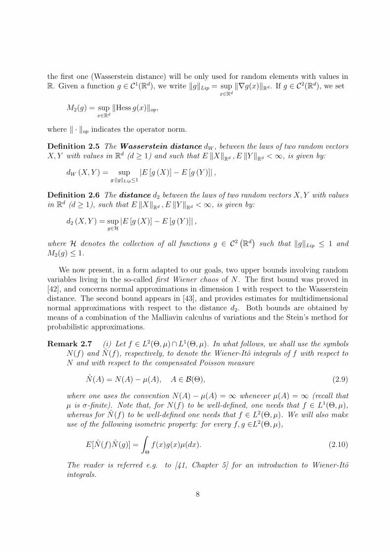
the first one (Wasserstein distance) will be only used for random elements with values inR. Given a function g ∈ C1(Rd), we write ‖g‖Lip = sup

x∈Rd

‖∇g(x)‖Rd. If g ∈ C2(Rd), we set

M2(g) = supx∈Rd

‖Hess g(x)‖op,

where ‖ · ‖op indicates the operator norm.

Definition 2.5 The Wasserstein distance dW , between the laws of two random vectorsX, Y with values in R

d (d ≥ 1) and such that E ‖X‖Rd , E ‖Y ‖

Rd <∞, is given by:

dW (X, Y ) = supg:‖g‖Lip≤1

|E [g (X)]−E [g (Y )]| ,

Definition 2.6 The distance d2 between the laws of two random vectors X, Y with valuesin R

d (d ≥ 1), such that E ‖X‖Rd , E ‖Y ‖

Rd <∞, is given by:

d2 (X, Y ) = supg∈H

|E [g (X)]−E [g (Y )]| ,

where H denotes the collection of all functions g ∈ C2(Rd)such that ‖g‖Lip ≤ 1 and

M2(g) ≤ 1.

We now present, in a form adapted to our goals, two upper bounds involving randomvariables living in the so-called first Wiener chaos of N . The first bound was proved in[42], and concerns normal approximations in dimension 1 with respect to the Wassersteindistance. The second bound appears in [43], and provides estimates for multidimensionalnormal approximations with respect to the distance d2. Both bounds are obtained bymeans of a combination of the Malliavin calculus of variations and the Stein’s method forprobabilistic approximations.

Remark 2.7 (i) Let f ∈ L2(Θ, µ)∩L1(Θ, µ). In what follows, we shall use the symbolsN(f) and N(f), respectively, to denote the Wiener-Ito integrals of f with respect toN and with respect to the compensated Poisson measure

N(A) = N(A)− µ(A), A ∈ B(Θ), (2.9)

where one uses the convention N(A) − µ(A) = ∞ whenever µ(A) = ∞ (recall thatµ is σ-finite). Note that, for N(f) to be well-defined, one needs that f ∈ L1(Θ, µ),whereas for N(f) to be well-defined one needs that f ∈ L2(Θ, µ). We will also makeuse of the following isometric property: for every f, g ∈L2(Θ, µ),

E[N(f)N(g)] =

∫

Θ

f(x)g(x)µ(dx). (2.10)

The reader is referred e.g. to [41, Chapter 5] for an introduction to Wiener-Itointegrals.

8

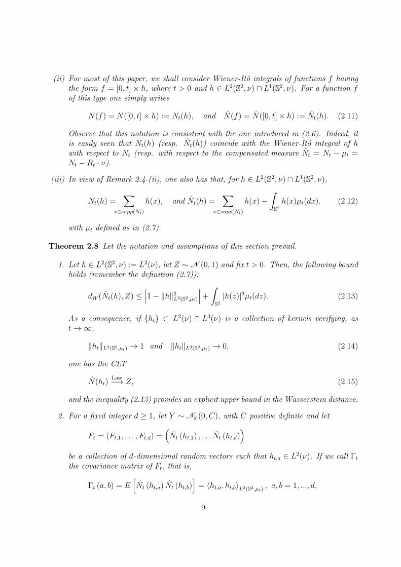
(ii) For most of this paper, we shall consider Wiener-Ito integrals of functions f havingthe form f = [0, t]× h, where t > 0 and h ∈ L2(S2, ν) ∩ L1(S2, ν). For a function fof this type one simply writes

N(f) = N([0, t]× h) := Nt(h), and N(f) = N([0, t]× h) := Nt(h). (2.11)

Observe that this notation is consistent with the one introduced in (2.6). Indeed, itis easily seen that Nt(h) (resp. Nt(h)) coincide with the Wiener-Ito integral of hwith respect to Nt (resp. with respect to the compensated measure Nt = Nt − µt =Nt −Rt · ν).

(iii) In view of Remark 2.4-(ii), one also has that, for h ∈ L2(S2, ν) ∩ L1(S2, ν),

Nt(h) =∑

x∈supp(Nt)

h(x), and Nt(h) =∑

x∈supp(Nt)

h(x)−∫

S2

h(x)µt(dx), (2.12)

with µt defined as in (2.7).

Theorem 2.8 Let the notation and assumptions of this section prevail.

1. Let h ∈ L2(S2, ν) := L2(ν), let Z ∼ N (0, 1) and fix t > 0. Then, the following boundholds (remember the definition (2.7)):

dW (Nt(h), Z) ≤∣∣∣1− ‖h‖2L2(S2,µt)

∣∣∣+∫

S2

|h(z)|3µt(dz). (2.13)

As a consequence, if ht ⊂ L2(ν) ∩ L3(ν) is a collection of kernels verifying, ast→ ∞,

‖ht‖L2(S2,µt) → 1 and ‖ht‖L3(S2,µt) → 0, (2.14)

one has the CLT

N(ht)Law−→ Z, (2.15)

and the inequality (2.13) provides an explicit upper bound in the Wasserstein distance.

2. For a fixed integer d ≥ 1, let Y ∼ Nd (0, C), with C positive definite and let

Ft = (Ft,1, . . . , Ft,d) =(Nt (ht,1) , . . . Nt (ht,d)

)

be a collection of d-dimensional random vectors such that ht,a ∈ L2(ν). If we call Γtthe covariance matrix of Ft, that is,

Γt (a, b) = E[Nt (ht,a) Nt (ht,b)

]= 〈ht,a, ht,b〉L2(S2,µt)

, a, b = 1, ..., d,

9

then:

d2 (Ft, Y ) ≤∥∥C−1

∥∥op‖C‖ 1

2op ‖C − Γt‖H.S. (2.16)

+

√2π

8

∥∥C−1∥∥ 3

2

op‖C‖op

d∑

i,j,k=1

∫

S2

|ht,i (x)| |ht,j (x)| |ht,k (x)|µt (dx) ,

≤∥∥C−1

∥∥op‖C‖ 1

2op ‖C − Γt‖H.S. (2.17)

+d2√2π

8

∥∥C−1∥∥ 3

2

op‖C‖op

d∑

i=1

∫

S2

|ht,i (x)|3 µt (dx) ,

where ‖ · ‖op and ‖ · ‖H.S. stand, respectively, for the operator and Hilbert-Schmidtnorms. In particular, if Γt (a, b) −→ C (a, b) and

∫S2|ht,a (x)|3 µt (dx) −→ 0 as t −→

∞, for a, b = 1, . . . d, then d2 (Ft, Y ) −→ 0 and Ft converges in distribution to Y .

Remark 2.9 The estimate (2.16) will be used to deduce one of the main multidimensionalbounds in the present paper. It is a direct consequence of Theorem 3.3 in [43], where thefollowing relation is proved: for every vector (F1, ..., Fd) of sufficiently regular centeredfunctionals of Nt,

d2(F,X) ≤∥∥C−1

∥∥op‖C‖1/2op

√√√√d∑

i,j

E

[C(i, j)− 〈DFi,−DL−1Fj〉L2(µt)

]2

+

√2π

8

∥∥C−1∥∥3/2op

‖C‖op∫

S2

µt(dz)E

(

d∑

i=1

|DzFi|)2( d∑

j=1

∣∣DzL−1Fj

∣∣) ,

where

DzF (ω) = Fz(ω)− F (ω) , a.e.− µ(dz)P (dω) ,

and

Fz(N) = Fz(N + δz),

that is, the random variable Fz is obtained by adding to the argument of F (which is afunction of the point measure N), a Dirac mass at z, and L−1 is the so-called pseudo-inverseof the Ornstein-Uhlenbeck operator. The estimate (2.16) is then obtained by observing that,when Fi = Ft,i = Nt(ht,i), then DzFi = −DzL

−1F = ht,i(z), in such a way that

√√√√d∑

i,j

E

[C(i, j)− 〈DFi,−DL−1Fj〉L2(µ)

]2= ‖C −Kt‖H.S. ,

10

and

∫

S2

µt(dz)E

(

d∑

i=1

|DzFi|)2( d∑

j=1

∣∣DzL−1Fj

∣∣)

=d∑

i,j,k=1

∫

S2

|ht,i (x)| |ht,j (x)| |ht,k (x)|µt (dx) .

The next statement deals with the interesting fact that the convergence in law impliedby Theorem 2.8 is indeed stable, as defined e.g. in the classic reference [19, Chapter 4].

Proposition 2.10 The central limit theorem described at the end of Point 2 of Theorem2.8 (and a fortiori the CLT at Point 1 of the same theorem) is stable with respect to σ(N)(the σ-field generated by N) in the following sense: for every random variable X that isσ(N)-measurable, one has that

(X,Ft)Law−→ (X, Y ),

where Y ∼ Nd(0, C) is independent of N .

Proof. We just deal with the case d = 1, the extension to a general d followingfrom elementary considerations. A density argument shows that it is enough to prove thefollowing claim: if N(hn) (hn ∈ L2(µ), n ≥ 1) is a sequence of random variables verifyingE[N(hn)

2] = ‖hn‖2L2(µ) → 1 and∫Θ|hn|3dµ → 0, then for every fixed f ∈ L2(µ), the pair

(N(f), N(hn)) converges in distribution, as n → ∞, to (N(f), Z), where Z ∼ N (0, 1) isindependent of N . To see this, we start with the explicit formula (see e.g. [41, formula(5.3.31)]): for every λ, γ ∈ R

ψn(λ, γ) := E[exp(iλN(f) + γN(hn))]

= exp

[∫

Θ

[eiλf(x)+iγhn(x)−1−i(λf(x) + γhn(x))

]µ(dx)

].

Our aim is to prove that, under the stated assumptions,

limn→∞

log(ψn(λ, γ)) =

∫

Θ

[eiλf(x) − 1− iλf(x)

]µ(dx)− γ2

2.

Standard computations show that∣∣∣ log(ψn(λ, γ))−

∫

Θ

[eiλf(x) − 1− iλf(x)

]µ(dx)− γ2

2

∣∣∣

≤∣∣∣γ

2

2− γ2

2

∫

Θ

hn(x)2µ(dx)

∣∣∣+ |γλ| |〈hn, f〉L2(µ)|+|γ|36

∫

Θ

|hn(x)|3µ(dx) .

Since∫Θ|hn(x)|3µ(dx) → 0 and the mapping n 7→ ‖hn‖2L2(µ) is bounded, one has that

〈hn, f〉L2(µ) → 0, and the conclusion follows by using the fact that ‖hn‖2L2(µ) → 1 byassumption.

11

3 Needlet coefficients

3.1 Background: the needlet construction

We now provide an overview of the construction of the set of needlets on the unit sphere.The reader is referred to [30, Chapter 10] for an introduction to this topic. Relevantreferences on this subject are: the seminal papers [35, 36], where needlets have beenfirst defined; [13, 14, 12, 15], among others, for generalizations to homogeneous spaces ofcompact groups and spin fiber bundles; [3, 4, 28, 32] for the analysis of needlets on sphericalGaussian fields, and [31, 46, 9, 11] for some (among many) applications to cosmological andastrophysical issues; see also [34, 49] for other approaches to spherical wavelets construction.

(Spherical harmonics) In Fourier analysis, the set of spherical harmonics

Ylm : l ≥ 0, m = −l, ..., l

provides an orthonormal basis for the space of square-integrable functions on the unitsphere L2 (S2, dx) := L2 (S2), where dx stands for the Lebesgue measure on S

2 (see forinstance [2, 23, 30, 51]). Spherical harmonics are defined as the eigenfunctions of thespherical Laplacian ∆S2 corresponding to eigenvalues −l (l + 1), e.g. ∆S2Ylm = −l(l +1)Ylm, see again [30, 51, 54] for analytic expressions and more details and properties. Forevery l ≥ 0, we define Kl as the linear space given by the restriction to the sphere of thepolynomials with degree at most l. Plainly, one has that

Kl =l⊕

k=0

span Ykm : m = −k, ..., k ,

where the direct sum is in the sense of L2 (S2).

(Cubature points) It is well-known that for every integer l = 1, 2, ... there exists a finite setof cubature points Ql ⊂ S

2, as well as a collection of weights λη, indexed by the elementsof Ql, such that

∀f ∈ Kl,

∫

S2

f(x)dx =∑

η∈Ql

ληf(η).

Now fix B > 1, and write [x] to indicate the integer part of a given real x. In what follows,we shall denote by Xj = ξjk and λjk, respectively, the set Q[2Bj+1] and the associatedclass of weights. We also write Kj = cardXj. As proved in [35, 36], cubature points andweights can be chosen to satisfy

λjk ≈ B−2j , Kj ≈ B2j , (3.18)

where by a ≈ b, we mean that there exists c1, c2 > 0 such that c1a ≤ b ≤ c2a (see also e.g.[5, 44, 45] and [30, Chapter 10]).

12

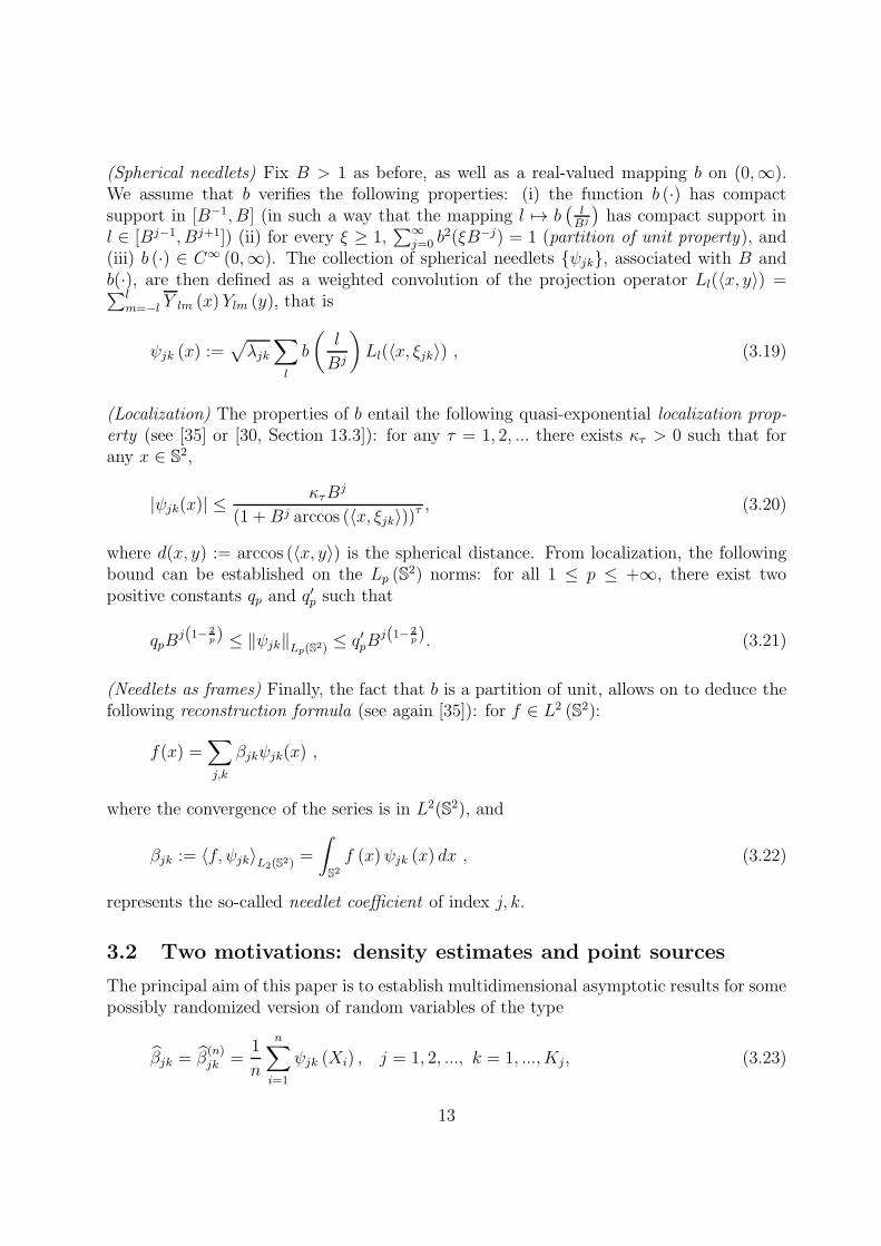
(Spherical needlets) Fix B > 1 as before, as well as a real-valued mapping b on (0,∞).We assume that b verifies the following properties: (i) the function b (·) has compactsupport in [B−1, B] (in such a way that the mapping l 7→ b

(lBj

)has compact support in

l ∈ [Bj−1, Bj+1]) (ii) for every ξ ≥ 1,∑∞

j=0 b2(ξB−j) = 1 (partition of unit property), and

(iii) b (·) ∈ C∞ (0,∞). The collection of spherical needlets ψjk, associated with B andb(·), are then defined as a weighted convolution of the projection operator Ll(〈x, y〉) =∑l

m=−l Y lm (x) Ylm (y), that is

ψjk (x) :=√λjk∑

l

b

(l

Bj

)Ll(〈x, ξjk〉) , (3.19)

(Localization) The properties of b entail the following quasi-exponential localization prop-erty (see [35] or [30, Section 13.3]): for any τ = 1, 2, ... there exists κτ > 0 such that forany x ∈ S

2,

|ψjk(x)| ≤κτB

j

(1 +Bj arccos (〈x, ξjk〉))τ, (3.20)

where d(x, y) := arccos (〈x, y〉) is the spherical distance. From localization, the followingbound can be established on the Lp (S

2) norms: for all 1 ≤ p ≤ +∞, there exist twopositive constants qp and q

′p such that

qpBj(1− 2

p) ≤ ‖ψjk‖Lp(S2)≤ q′pB

j(1− 2p). (3.21)

(Needlets as frames) Finally, the fact that b is a partition of unit, allows on to deduce thefollowing reconstruction formula (see again [35]): for f ∈ L2 (S2):

f(x) =∑

j,k

βjkψjk(x) ,

where the convergence of the series is in L2(S2), and

βjk := 〈f, ψjk〉L2(S2)=

∫

S2

f (x)ψjk (x) dx , (3.22)

represents the so-called needlet coefficient of index j, k.

3.2 Two motivations: density estimates and point sources

The principal aim of this paper is to establish multidimensional asymptotic results for somepossibly randomized version of random variables of the type

βjk = β(n)jk =

1

n

n∑

i=1

ψjk (Xi) , j = 1, 2, ..., k = 1, ..., Kj, (3.23)

13

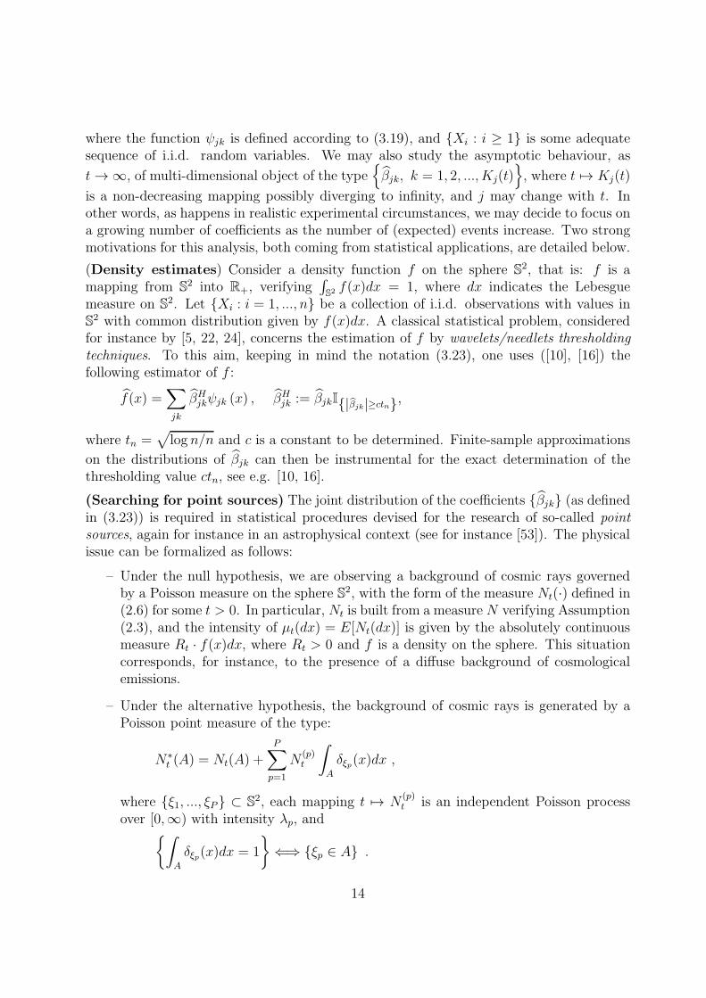
where the function ψjk is defined according to (3.19), and Xi : i ≥ 1 is some adequatesequence of i.i.d. random variables. We may also study the asymptotic behaviour, as

t→ ∞, of multi-dimensional object of the typeβjk, k = 1, 2, ..., Kj(t)

, where t 7→ Kj(t)

is a non-decreasing mapping possibly diverging to infinity, and j may change with t. Inother words, as happens in realistic experimental circumstances, we may decide to focus ona growing number of coefficients as the number of (expected) events increase. Two strongmotivations for this analysis, both coming from statistical applications, are detailed below.

(Density estimates) Consider a density function f on the sphere S2, that is: f is a

mapping from S2 into R+, verifying

∫S2f(x)dx = 1, where dx indicates the Lebesgue

measure on S2. Let Xi : i = 1, ..., n be a collection of i.i.d. observations with values in

S2 with common distribution given by f(x)dx. A classical statistical problem, considered

for instance by [5, 22, 24], concerns the estimation of f by wavelets/needlets thresholdingtechniques. To this aim, keeping in mind the notation (3.23), one uses ([10], [16]) thefollowing estimator of f :

f(x) =∑

jk

βHjkψjk (x) , βHjk := βjkI|βjk|≥ctn,

where tn =√log n/n and c is a constant to be determined. Finite-sample approximations

on the distributions of βjk can then be instrumental for the exact determination of thethresholding value ctn, see e.g. [10, 16].

(Searching for point sources) The joint distribution of the coefficients βjk (as definedin (3.23)) is required in statistical procedures devised for the research of so-called pointsources, again for instance in an astrophysical context (see for instance [53]). The physicalissue can be formalized as follows:

– Under the null hypothesis, we are observing a background of cosmic rays governedby a Poisson measure on the sphere S2, with the form of the measure Nt(·) defined in(2.6) for some t > 0. In particular, Nt is built from a measure N verifying Assumption(2.3), and the intensity of µt(dx) = E[Nt(dx)] is given by the absolutely continuousmeasure Rt · f(x)dx, where Rt > 0 and f is a density on the sphere. This situationcorresponds, for instance, to the presence of a diffuse background of cosmologicalemissions.

– Under the alternative hypothesis, the background of cosmic rays is generated by aPoisson point measure of the type:

N∗t (A) = Nt(A) +

P∑

p=1

N(p)t

∫

A

δξp(x)dx ,

where ξ1, ..., ξP ⊂ S2, each mapping t 7→ N

(p)t is an independent Poisson process

over [0,∞) with intensity λp, and∫

A

δξp(x)dx = 1

⇐⇒ ξp ∈ A .

14

In this case, one has that N∗t is a Poisson measure with atomic intensity

µ∗t (A) := E[N∗

t (A)] = Rt

∫

A

f(x)dx+

P∑

p=1

λpt ·∫

A

δξp(x)dx .

In this context, the informal expression “searching for point sources” can then be trans-lated into “testing for P = 0” or “jointly testing for λp > 0 at p = 1, ..., P”. The numberP and the locations ξ1, ...ξP can be in general known or unknown. We refer to [18, 52]for astrophysical applications of these ideas.

Remark 3.1 In order to directly apply the findings of [42, 43], in what follows we shallfocus on a randomized version of (3.23), where n is replaced by an independent Poissonnumber whose parameter diverges to infinity. Also, we will prefer a deterministic normal-ization over a random one. As formally shown in the discussion to follow, the resultingrandomized coefficients can be neatly put into the framework of Section 2.

3.3 Needlet coefficients as Wiener-Ito integrals

Let N be a Poisson measure on R+ × S2 satisfying the requirements of Assumption 2.3

(in particular, the intensity of N has the form ρ × ν, where ν(dx) = f(x)dx, for someprobability density f on the sphere, and one writes Rt = ρ([0, t]), t > 0). For everyt > 0, let the Poisson measure Nt on S

2 be defined as in (2.6). For every j ≥ 1 and everyk = 1, ..., Nj, consider the function ψjk defined in (3.19), and observe that ψjk is triviallyan element of L3(S2, ν) ∩ L2(S2, ν) ∩ L1(S2, ν). We write

σ2jk :=

∫

S2

ψ2jk (x) f(x)dx , bjk :=

∫

S2

ψjk (x) f(x)dx .

Observe that, if f(x) = 14π

(that is, the uniform density on the sphere), then bjk = 0 forevery j > 1. On the other hand, under (2.8),

ζ1 ‖ψjk (.)‖2L2 ≤ σ2jk ≤ ζ2 ‖ψjk (.)‖2L2 . (3.24)

Note that (see 3.21) the L2-norm of ψjk is uniformly bounded above and below, andtherefore the same is true for

σ2jk

(indeed, there exists κ > 0, independent of j and k,

such that 0 < κ < ‖ψjk‖2L2(S2) < 1). For every t > 0 and every j, k, we introduce the kernel

h(Rt)jk (x) =

ψjk (x)√Rtσjk

, x ∈ S2 , (3.25)

and write

β(Rt)jk := Nt

(h(Rt)jk

)=

∫

S2

h(Rt)jk (x) Nt (dx) =

∑

x∈supp(Nt)

h(Rt)jk (x)−Rt ·

∫

S2

h(Rt)jk (x)ν(dx) , (3.26)

15

In view of Remark 2.4-(ii), the random variable β(Rt)jk can always be represented in the form

β(Rt)jk =

(∑Nt(S2)i=1 ψjk (Xi)−Rtbjk

)

√Rtσjk

,

where Xi : i ≥ 1 is a sequence of i.i.d. random variables with common distribution ν,and independent of the Poisson random variable Nt(S

2). Moreover, the following relationsare immediately checked:

Eβ(Rt)jk = 0, E[(β

(Rt)jk )2] = 1 . (3.27)

Remark 3.2 Using the notation (3.23), we have that

β(Rt)jk =

(Nt(S

2)× β(Nt(S2))jk − Rtbjk

)

√Rtσjk

.

4 Bounds in dimension one

We are now going to apply the content of Theorem 2.8-(1) to the random variables β(Rt)jk

introduced in the previous section. In the next statement, we write Z ∼ N (0, 1) to indicatea centered Gaussian random variable with unit variance. Recall that ζ2 := supx∈S2 |f (x)|,p ≥ 1, and that the constants qp, q

′p have been defined in (3.21).

Proposition 4.1 For every j, k and every t > 0, one has that

dW

(β(Rt)jk , Z

)≤ (q′3)

3ζ2Bj

√Rtσ3

jk

.

It follows that for any sequence (j(n), k(n), t(n)), β(Rt(n))j(n)k(n) converges in distribution to Z,

as n → ∞, provided B2j(n) = o(Rt(n)). The convergence is σ(N)-stable, in the sense ofProposition 2.10.

Proof. Using (3.25)–(3.26) together with (2.17) and (2.8),

dW

(β(Rt)jk , Z

)≤

∫

S2

∣∣∣h(Rt)jk (x)

∣∣∣3

µt (dx)

=Rt√R3tσ

3jk

∫

S2

|ψjk (x)|3 f (x) dx ≤ ζ2√Rtσ

3jk

‖ψjk‖3L3(S2)

≤ (q′3)3ζ2B

j

√Rtσ3

jk

,

where in the last inequality we use the property (3.21) with p = 3 to have:

‖ψjk‖3L3(S2) ≤ (q′3)3B3j(1− 2

3) = (q′3)3Bj .

16

The last part of the statement follows from the fact that the topology induced by theWasserstein distance (on the class of probability distributions on the real line) is strictlystronger than the topology of convergence in law.

Remark 4.2 For f(x) ≡ 4π−1 we have

σ2jk =

1

4π

∫

S2

ψ2jk (x) dx = ‖ψjk‖2L2(S2) ,

and more generally, under (2.8),

dW

(β(Rt)jk , Z

)≤ Bj

√Rt

(q′3)3ζ2

ζ3/21 ‖ψjk‖3/2L2(S2)

:= γ(j, k, t) . (4.28)

Remark 4.3 The previous result can be given the following heuristic interpretation. Thefactor B−j can be viewed as the “effective scale” of the wavelet, i.e. it is the radius ofthe region centred at ξjk where the value of the wavelet function is not negligible. Becauseneedlets are isotropic, the “effective area” is of order B−2j . For governing measures withdensity which is bounded and bounded away from zero, the expected number of observationson a spherical cap of radius B−j around ξjk is hence given by

E[card

Xi : d(Xi, ξjk) ≤ B−j

]≃ Rt

∫

d(x,ξjk)≤B−j

f(x)dx ,

ζ1B−2jRt ≤ Rt

∫

d(x,ξjk)≤B−j

f(x)dx ≤ ζ2B−2jRt ,

using [4, equation (8)]. Because the Central Limit Theorem can hold only when the effectivenumber of observations grows to infinity, the condition B−2jRt → ∞ is quite expected. Inthe thresholding literature, coefficients are usually considered up to the frequency JR suchthat B2JR ≃ Rt/ logRt, see for instance [16] and [5]; under these circumstances, we have

d2

(β(Rt)JRk

, Z)= O

(1√

logRt

)−→ 0 for Rt −→ +∞ .

Therefore β(Rt)JRk

does converge in law to Z.

5 Multidimensional bounds

We are now going to apply Part 2 of Theorem (2.8) to the computation of multidimensionalBerry-Esseen bounds involving vectors of needlet coefficients of the type (3.26). Afterhaving proved some technical estimates in Section 5.1, we will consider two bounds. Oneis proved in Section 5.2 by means of (2.17), and it is well adapted to the case where thenumber of needlet coefficients, say d, is fixed. In Section 5.3, we shall focus on (2.16), anddeduce a bound which is adapted to the case where the number d is possibly growing toinfinity.

17

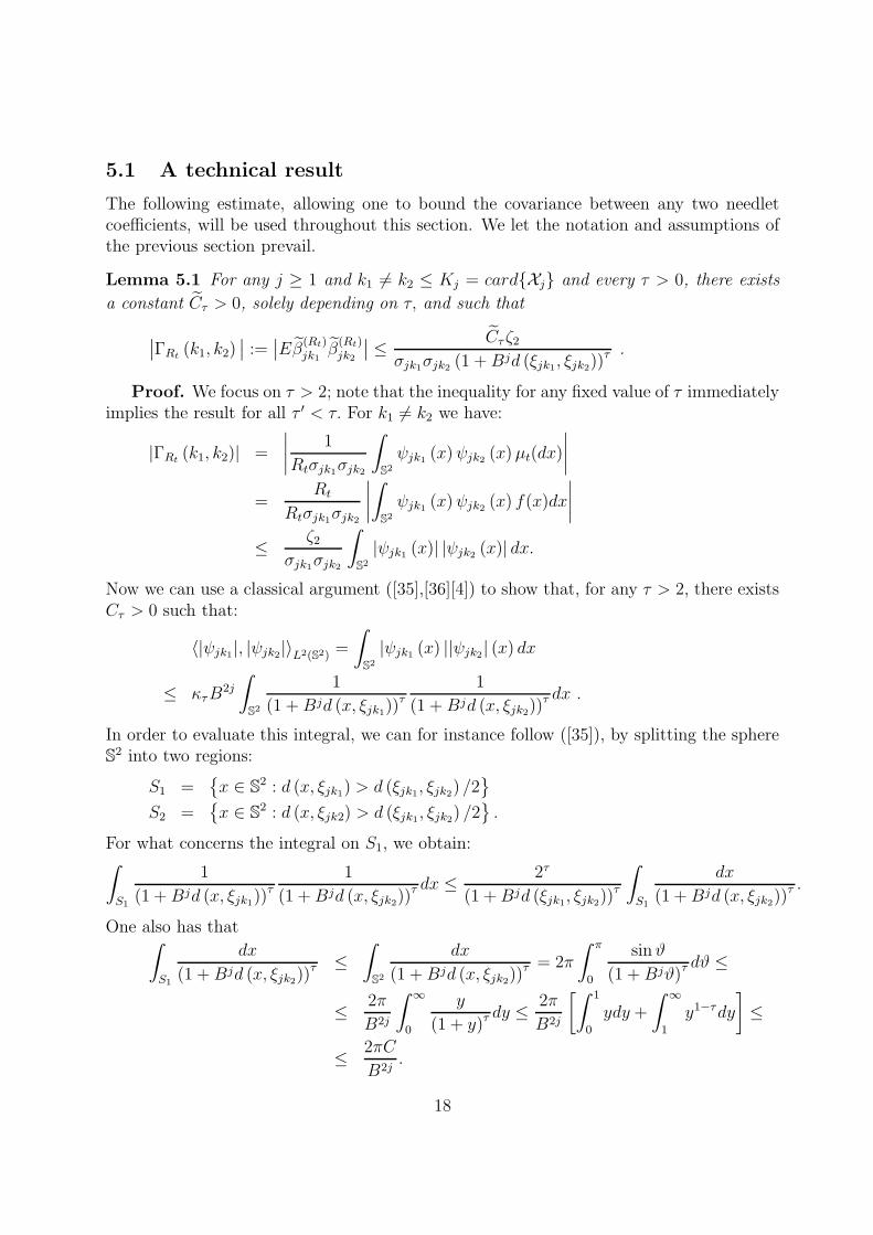
5.1 A technical result

The following estimate, allowing one to bound the covariance between any two needletcoefficients, will be used throughout this section. We let the notation and assumptions ofthe previous section prevail.

Lemma 5.1 For any j ≥ 1 and k1 6= k2 ≤ Kj = cardXj and every τ > 0, there exists

a constant Cτ > 0, solely depending on τ, and such that

∣∣ΓRt(k1, k2)

∣∣ :=∣∣Eβ(Rt)

jk1β(Rt)jk2

∣∣ ≤ Cτζ2σjk1σjk2 (1 +Bjd (ξjk1, ξjk2))

τ .

Proof. We focus on τ > 2; note that the inequality for any fixed value of τ immediatelyimplies the result for all τ ′ < τ. For k1 6= k2 we have:

|ΓRt(k1, k2)| =

∣∣∣∣1

Rtσjk1σjk2

∫

S2

ψjk1 (x)ψjk2 (x)µt(dx)

∣∣∣∣

=Rt

Rtσjk1σjk2

∣∣∣∣∫

S2

ψjk1 (x)ψjk2 (x) f(x)dx

∣∣∣∣

≤ ζ2σjk1σjk2

∫

S2

|ψjk1 (x)| |ψjk2 (x)| dx.

Now we can use a classical argument ([35],[36][4]) to show that, for any τ > 2, there existsCτ > 0 such that:

〈|ψjk1|, |ψjk2|〉L2(S2) =

∫

S2

|ψjk1 (x) ||ψjk2| (x) dx

≤ κτB2j

∫

S2

1

(1 +Bjd (x, ξjk1))τ

1

(1 +Bjd (x, ξjk2))τ dx .

In order to evaluate this integral, we can for instance follow ([35]), by splitting the sphereS2 into two regions:

S1 =x ∈ S

2 : d (x, ξjk1) > d (ξjk1, ξjk2) /2

S2 =x ∈ S

2 : d (x, ξjk2) > d (ξjk1, ξjk2) /2.

For what concerns the integral on S1, we obtain:∫

S1

1

(1 +Bjd (x, ξjk1))τ

1

(1 +Bjd (x, ξjk2))τ dx ≤ 2τ

(1 +Bjd (ξjk1, ξjk2))τ

∫

S1

dx

(1 +Bjd (x, ξjk2))τ .

One also has that∫

S1

dx

(1 +Bjd (x, ξjk2))τ ≤

∫

S2

dx

(1 +Bjd (x, ξjk2))τ = 2π

∫ π

0

sinϑ

(1 +Bjϑ)τdϑ ≤

≤ 2π

B2j

∫ ∞

0

y

(1 + y)τdy ≤ 2π

B2j

[∫ 1

0

ydy +

∫ ∞

1

y1−τdy

]≤

≤ 2πC

B2j.

18

Because calculations on the region S2 are exactly the same and because S2 ⊂ S1 ∪ S2, we

have that, for some constant Cτ depending on τ ,

〈|ψjk1|, |ψjk2|〉L2(S2) ≤Cτ

(1 +Bjd (ξjk1, ξjk2))τ ,

yielding the desired conclusion.

Remark 5.2 Assuming that d (ξjk1, ξjk2) > δ uniformly for all j, we have immediately

∣∣Eβ(Rt)jk1

β(Rt)jk2

∣∣ ≤ κ′τ,ζ2 × B−jτ ,

where the constant κ′τ,ζ2 only depend on τ, ζ2.

Remark 5.3 The previous Lemma provides a tight bound, of some independent interest,on the high frequency behaviour of covariances among wavelet coefficients for Poisson ran-dom fields. For Gaussian isotropic random fields, analogous results were provided by [3],in the case of standard needlets (bounded support), and by [28]–[32], in the “Mexican” casewhere support may be unbounded in multipole space. It should be noted how asymptotic un-correlation holds in much greater generality for Poisson random fields than for Gaussianfield: indeed in the latter case a regular variation condition had to be imposed on the tailbehaviour of the angular power spectrum, and in the Mexican case this condition had to bestrengthened imposing an upper bound on the decay of the spectrum itself. The reason forsuch discrepancy is easily understood: for Poisson random fields, non overlapping regionsare independent, whence (heuristically) localization in pixel space is sufficient to ensureasymptotic uncorrelation; on the contrary, in the Gaussian isotropic case different regionsof the field are correlated at any angular distance, and asymptotic uncorrelation for thecoefficients requires a much more delicate cancellation argument.

5.2 Fixed dimension

Fix d ≥ 2 and j ≥ 1, consider a fixed number of sampling points ξjk1, ..., ξjkd, and definethe associated d-dimensional vector

β(Rt)j· :=

(β(Rt)jk1

, ..., β(Rt)jkd

),

whose covariance matrix will be denoted by Γt (note that, by construction, Γt(i, i) = 1 forevery i = 1, ..., d). Our aim is to apply the rough bound (2.17) in order to estimate the

distance between the law of β(Rt)j· and the law of a random Gaussian vector Z ∼ Nd(0, Id),

where C = Id stands for the identity d×d matrix. Using Lemma 5.1, one has the followingbasic estimates:

19

∥∥C−1∥∥op

= ‖C‖ 12op = 1 ,

‖C − Γt‖H.S. ≤

√√√√d∑

k1 6=k2=1

E[β(Rt)jk1

β(Rt)jk2

]2

≤ d supk1 6=k2=1,...,d

1

σjk1σjk2

Cτζ2(1 +Bjd (ξjk1, ξjk2))

τ

≤ d

ζ1q22

× Cτζ2(1 +Bj infk1 6=k2=1,...,d d (ξjk1, ξjk2))

τ = A(t) . (5.29)

Applying (2.17) yields therefore that

d2

(β(Rt)j , Z

)≤ A(t) + d2

√2π

8

d∑

k=1

Rt

∫

S2

∣∣∣h(Rt)jk (x)

∣∣∣3

f (x) dx

= A(t) + d2√2π

8

ζ2Rt√R3t

d∑

k=1

∫

S2

|ψjk (x)|3σ3jk

dx

≤ A(t) +d3ζ2√Rtζ

3/21 q32

√2π

8‖ψjk‖3L3(S2)

≤ A(t) +(q′3)

3d3ζ2√Rtζ

3/21 q32

√2π

8Bj,

where we used (3.21) and (3.24) to yield σ3jk ≥ ζ

3/21 q32. We write this result as a separate

statement.

Proposition 5.4 Under the above notation and assumptions,

d2

(β(Rt)j , Z

)≤ dCτζ2B

−jτ

ζ1q22 (1 + infk1 6=k2=1,...,d d (ξjk1, ξjk2))τ +

(q′3)3d3ζ2√

Rtζ3/21 q32

√2π

8Bj .

Because τ can be chosen arbitrarily large, it is immediately seen that the leading termin the d2 distance is decaying with the same rate as in the univariate case, e.g. Bj/

√Rt.

Assuming however that d = dt, i.e. the case where the number of coefficients is itselfgrowing with t, the previous bound may become too large to be applicable. We shall hencetry to establish a tighter bound, as detailed in the next section.

20

5.3 Growing dimension

In this section we allow for a growing number of coefficients to be evaluated simultaneously,and investigate the bounds that can be obtained under these circumstances. More precisely,we are now focussing on

β(Rt)j(t)· :=

(β(Rt)j(t)k1

, ..., β(Rt)j(t)kdt

),

where dt → ∞, as t → ∞. Throughout the sequel, we shall assume that the points atwhich these coefficients are evaluated satisfy the condition:

infk1 6=k2=1,...,dt

d(ξj(t)k1 , ξj(t)k2

)≈ 1√

dt. (5.30)

Condition (5.30) is rather minimal; in fact, the cubature points for a standard needlet/waveletconstruction can be taken to form a maximal (dt)

−1/2-net (see [4, 13, 35, 44] for more detailsand discussion). The following result is the main achievement of the paper.

Theorem 5.5 Let the previous assumptions and notation prevail. Then for all τ = 2, 3...,there exist positive constants c and c′, (depending on τ, ζ1, ζ2 but not from t, j(t), d(t)) suchthat we have

d2

(β(Rt)j(t). , Z

)≤ cdt(

1 +Bj(t) infk1 6=k2=1,...,dt d(ξj(t)k1, ξj(t)k2

))τ +√2π

8

c′dtBj(t)

ζ3/21 q32

√Rt

. (5.31)

Proof. In view of (2.16) and (5.29), we just have to prove that the quantity

√2π

8

Rt

ζ3/21 q32

√R3t

dt∑

k1k2k3

∫

S2

∣∣ψj(t)k1 (z)∣∣ ∣∣ψj(t)k2 (z)

∣∣ ∣∣ψj(t)k3 (z)∣∣ f(z)dz

is smaller than the second summand on the RHS of (5.31). Now note that

dt∑

k1k2k3

∫

S2

∣∣ψj(t)k1 (z)∣∣ ∣∣ψj(t)k2 (z)

∣∣ ∣∣ψj(t)k3 (z)∣∣ dz ≤

∑

λ

∫

B(ξj(t)λ,B−j(t))

dt∑

k

∣∣ψj(t)k (z)∣∣3

dz ,

where, for any z ∈ B(ξj(t)λ, B−j(t))

dt∑

k

∣∣ψj(t)k (z)∣∣ ≤

dt∑

k

CτBj(t)

1 +Bj(t)d(ξj(t)k, z)

τ

≤ CτBj(t) +

dt∑

k:ξj(t)k /∈B(ξj(t)λ,B−j(t))

CτBj(t)

1 +Bj(t)

[d(ξj(t)k, ξj(t)λ)− d(z, ξj(t)λ)

]τ

≤ CτBj(t) +

dt∑

k:ξj(t)k /∈B(ξj(t)λ,B−j(t))

CτBj(t)

Bj(t)d(ξj(t)k, ξj(t)λ)

τ .

21

Now for ξj(t)k /∈ B(ξj(t)λ, B−j(t)), x ∈ B(ξj(t)k, B−j(t)), we have by triangle inequality

d(ξj(t)k, ξj(t)λ) + d(ξj(t)k, x) ≥ d(ξj(t)λ, x),

and because

d(ξj(t)k, ξj(t)λ) ≥ d(ξj(t)k, x), and 2d(ξj(t)k, ξj(t)λ) ≥ d(ξj(t)λ, x) ,

we obtaindt∑

k:ξj(t)k /∈B(ξj(t)λ,B−j(t))

CτBj(t)

Bj(t)d(ξj(t)k, ξj(t)λ)

τ

=dt∑

k:ξj(t)k /∈B(ξj(t)λ,B−j(t))

1

meas(B(ξj(t)k, B−j(t)))

∫

B(ξj(t)k ,B−j(t))

κτBj(t)

Bj(t)d(ξj(t)k, ξj(t)λ)

τ dx

≤dt∑

k:ξj(t)k /∈B(ξj(t)λ,B−j(t))

1

meas(B(ξj(t)k, B−j(t)))

∫

B(ξj(t)k ,B−j(t))

κτ2τBj(t)

Bj(t)d(ξj(t)λ, x)

τ dx ≤ κ′τBj(t) ,

arguing as in [3], Lemma 6. Hence

dt∑

k

∣∣ψj(t)k (z)∣∣ ≤ κ′′τB

j(t) , (5.32)

uniformly over z ∈ S2, which immediately provides the bound.

∑

λ

∫

B(ξj(t)λ,B−j)

dt∑

k

∣∣ψj(t)k (z)∣∣3

dz ≤ (κ′′τBj)3∑

λ

∫

B(ξj(t)λ,B−j(t))

dz = (κ′′′Bj(t))3 .

Finally, to establish the sharper constraint

∫

S2

dt∑

k

∣∣ψj(t)k (z)∣∣3

dz ≤ κτdtBj(t),

it is sufficient to note that, exploiting (5.32)∑

k1

∫

S2

∣∣ψj(t)k1 (z)∣∣∑

k2

∣∣ψj(t)k2 (z)∣∣∑

k3

∣∣ψj(t)k3 (z)∣∣ dz

≤ κ2B2j(t)dt∑

k1

∫

S2

∣∣ψj(t)k1 (z)∣∣ dz = κ2B2j(t)dj(t)

∥∥ψj(t)k∥∥L1(S2)

≤ dtκ2B2j(t)B−j(t) = dtκ

2Bj(t) ,

where we have used again∥∥ψj(t)k

∥∥pLp(S2)

= O(B2j(t)( 12− 1

p)p) = O(Bj(t)(p−2)), for p = 1. Thus

(5.31) is established.For definiteness, we shall also impose tighter conditions on the rate of growth of dt, B

j(t)

with respect to Rt, so that we can obtain a much more explicit bound, as follows:

22

Corollary 5.6 Let the previous assumptions and notation prevail, and assume moreoverthat there exists α, β such that, as t→ ∞

B2j(t) ≈ Rαt , 0 < α < 1 , dt ≈ Rβ

t , 0 < β < α .

There exists a constant κ (depending on ζ1, ζ2, but not on j, dj, B) such that

d2

(β(Rt)j(t). , Z

)≤ κ

dtBj(t)

√Rt

, (5.33)

for all vectors(β(Rt)jk1

, ..., β(Rt)jkdt

), such that (5.30) holds.

Proof. It suffices to note that

dtκ′τ,ζ2

(1 +Bj(t) infk1 6=k2=1,...,dt d (ξjk1, ξjk2))τ = O(B−τj(t)d

1+τ/2t )

= O

(dtB

j(t)

√Rt

(Rtd

τt

B(τ+1)2j(t)

)1/2)

and

Rtdτt

B(τ+1)2j(t)=

R1+βτt

R(τ+1)αt

= R−α+τ(β−α)+1t = o(1) , for τ >

1− α

α− β.

Remark 5.7 From (5.33), it follows that for Rt ≃ 1012 we can establish asymptotic joint

Gaussianity for all sequences of coefficients(β(Rt)j(t)k1(t)

, ..., β(Rt)j(t)kd(t)

) of dimensions such that

dtBj(t)

√Rt

= o(1) ,

e.g. we can take dt ≃ o(√Rt/B

j(t)) ≃ o(106/Bj(t)), so that even at multipoles in the orderof Bj(t) = O(103) we might take around 103 coefficients with the multivariate Gaussianapproximation still holding. These arrays would not be sufficient for the map reconstructionat this scale, but would indeed provide a basis for joint multiple testing procedures as thosedescribed earlier.

Remark 5.8 Assume that dt scales as B2j(t); loosely speaking, this corresponds to the sit-

uation when one focusses on the whole set of coefficients corresponding to scale j, so thatexact reconstruction for bandlimited functions with l = O(Bj) is feasible. Under this re-quirement, however, the ”covariance” term A(t), i.e. the first element on the right-handside of (5.31), is no longer asymptotically negligible and the approximation with Gaus-sian independent variables cannot be expected to hold. The approximation may however

23

be implemented in terms of a Gaussian vector with dependent components. For the sec-ond term, convergence to zero when dj(t) ≈ B2j(t) requires B3j(t) = o(

√Rt). In terms of

astrophysical applications, for Rt ≃ 1012 this implies that one can focus on scales until180/Bj ≃ 180/102 ≃ 2; this is close to the resolution level considered for ground-basedCosmic Rays experiments such as ARGO-YBJ ([18]). Of course, this value is much lowerthan the factor Bj = o(

√Rt) = o(106) required for the Gaussian approximation to hold

in the one-dimensional case (e.g., on a univariate sequence of coefficients, for instancecorresponding to a single location on the sphere).

Remark 5.9 As mentioned in the introduction, in this paper we decided to focus on a spe-cific framework (spherical Poisson fields), which we believe of interest from the theoreticaland the applied point of view. It is readily verified, however, how our results continue tohold with trivial modifications in a much greater span of circumstances, indeed in somecases with simpler proofs. Assume for instance we observe a sample of i.i.d. random vari-ables Xt , with probability density function f(.) which is bounded and has support in[a, b] ⊂ R. Consider the kernel estimates

fn(xnk) :=1

nB−j

n∑

t=1

K(Xt − xnkB−j

) , (5.34)

where K(.) denotes a compactly supported and bounded kernel satisfying standard regularityconditions, and for each j the evaluation points (xn0, ..., xnBj ) form a B−j-net; for instance

a = xn0 < xn1... < xnBj = b , xnk = a + kb− a

Bj, k = 0, 1, ..., Bj .

As argued earlier, conditionally on Nt([a, b]) = n, (5.34) has the same distribution as

fNt(xnk) :=

1

Nt[a, b]B−j

∫ b

a

K(u− xnkB−j

)dNt(u) ,

where Nt is a Poisson measure governed by Rt ×∫Af(x)dx for all A ⊂ [a, b]. Considering

that Nt

Rt→a.s. 1, a bound analogous to 5.33 can be established with little efforts for the vec-

tor fn(xn.) :=fn(xn1), ..., fn(xnBj )

. We leave this and related developments for further

research.

References

[1] Adell, J. A. and Lekuona, A. (2005), Sharp estimates in signed Poisson approximationof Poisson mixtures. Bernoulli 11(1), 47-65.

[2] Adler, R. J., Taylor, Jonathan E. (2007) Random Fields and Geometry, SpringerMonographs in Mathematics. Springer, New York.

24

[3] Baldi, P., Kerkyacharian, G., Marinucci, D. and Picard, D. (2009), Asymptotics forSpherical Needlets, Annals of Statistics, Vol. 37, No. 3, 1150-1171

[4] Baldi, P., Kerkyacharian, G., Marinucci, D. and Picard, D. (2009), SubsamplingNeedlet Coefficients on the Sphere, Bernoulli, Vol. 15, 438-463, arXiv: 0706.4169

[5] Baldi, P., Kerkyacharian, G., Marinucci, D. and Picard, D. (2009), Adaptive DensityEstimation for directional Data Using Needlets, Annals of Statistics, Vol. 37, No. 6A,3362-3395, arXiv: 0807.5059

[6] Bentkus, V. (2003). On the dependence of the Berry-Esseen bound on dimension.Journal of Statistical Planning and Inference 113, 385-402.

[7] Bourguin, S. and Peccati, G. (2012). A portmanteau inequality on the Poisson space.Preprint.

[8] Chen, L. H. Y. , Goldstein, L. and Shao, Q.-M. (2011), Normal Approximation byStein’s Method. Springer-Verlag.

[9] Delabrouille, J., Cardoso, J.-F., Le Jeune, M. , Betoule, M., Fay, G., Guilloux, F.(2008) A Full Sky, Low Foreground, High Resolution CMB Map from WMAP, As-tronomy and Astrophysics, Volume 493, Issue 3, 2009, pp.835-857, arXiv 0807.0773

[10] Donoho, D., Johnstone, I., Kerkyacharian, G. and Picard, D. (1996), Density estima-tion by wavelet thresholding, Annals of Statistics, 24, 508-539

[11] Feeney, S.M., Johnson, M.C., Mortlock, D.J. and Peiris, H.V. (2011), First observa-tional tests of eternal inflation: Analysis methods and WMAP 7-year results, PhysicalReview D, vol. 84, Issue 4, id. 043507

[12] Geller, D. and Marinucci, D. (2010) Spin Wavelets on the Sphere, Journal of FourierAnalysis and its Applications, 16, N.6, 840-884, arXiv: 0811.2835

[13] Geller, D. and Mayeli, A. (2009), Continuous Wavelets on Manifolds, MathematischeZeitschrift, Vol. 262, pp. 895-927, arXiv: math/0602201

[14] Geller, D. and Mayeli, A. (2009), Nearly Tight Frames and Space-Frequency Analy-sis on Compact Manifolds, Mathematische Zeitschrift, Vol, 263 (2009), pp. 235-264,arXiv: 0706.3642

[15] Geller, D. and Pesenson, I . (2011), Band-Limited Localized Parseval Frames andBesov Spaces on Compact Homogeneous Manifolds, Journal of Geometric Analysis,vol. 21, pp.334-371, arXiv:1002.3841

[16] Hardle, W., Kerkyacharian, G., Picard, D., and Tsybakov, A. (1997), Wavelets, Ap-proximations and Statistical Applications, Springer, Berlin

25

[17] Huang, C., Wang, H. and Zhang, L. Berry-Esseen bounds for kernel estimates ofstationary processes (2011), Journal of Statistical Planning and Inference, 141, no. 3,1290–1296

[18] Iuppa, R., Di Sciascio, G., Hansen, F.K., Marinucci, D. and Santonico, R., (2012)A Needlet-Based Approach to the Shower-Mode Data Analysis in the ARGO-YBJExperiment, Nuclear Instruments and Methods in Physics Research, Section A, inpress.

[19] Jacod J. and Shiryaev A.N. (1987), Limit Theorems for Stochastic Processes. Springer,Berlin.

[20] Jupp, P. E. (2005), Sobolev tests of goodness of fit of distributions on compact Rie-mannian manifolds. Annals of Statistics, Vol. 33 , no. 6, 2957-2966.

[21] Jupp, P. E.(2008), Data-driven Sobolev tests of uniformity on compact Riemannianmanifolds. Annals of Statistics, Vol. 36 (2008), no. 3, 1246-1260.

[22] Kerkyacharian, G., Pham Ngoc, T.M., Picard, D. (2011), Localized Spherical Decon-volution, Annals of Statistics, Vol. 39, no. 2, 1042–1068

[23] Koo, J.-Y. and Kim, P.T. (2008) Sharp Adaptation for Spherical Inverse Problemswith Applications to Medical Imaging, Journal of Multivariate Analysis, 99, 165-190

[24] Kueh, A. (2011), Locally Adaptive Density Estimation on the Unit Sphere UsingNeedlets, arXiv preprint 1004.1807

[25] Lachieze-Rey, R. and Peccati, G. (2011). Fine Gaussian fluctuations on the Poissonspace I: contractions, cumulants and geometric random graphs. Preprint.

[26] Lachieze-Rey, R. and Peccati, G. (2012). Fine Gaussian fluctuations on the Poissonspace II: rescaled kernels, marked processes and geometric U -statistics. Preprint.

[27] Last, G., Penrose, M., Schulte, M., Thale, C. (2012). Moments and central limittheorems for some multivariate Poisson functionals. Preprint.

[28] Lan, X. and Marinucci, D. (2008) On the Dependence Structure of Wavelet Coefficientsfor Spherical Random Fields, Stochastic Processes and their Applications, 119, 3749-3766, arXiv:0805.4154

[29] Li, Y., Wei, C., and Xing, G. (2011) Berry-Esseen bounds for wavelet estimator in aregression model with linear process errors, Statist. Probab. Lett., 81, no. 1, 103–110

[30] Marinucci, D. and Peccati, G. (2011), Random Fields on the Sphere. Representation,Limit Theorems and Cosmological Applications. Lecture Notes of the London Mathe-matical Society, 389. Cambridge University Press.

26

[31] Marinucci, D., Pietrobon, D., Balbi, A., Baldi, P., Cabella, P., Kerkyacharian, G.,Natoli, P. Picard, D., Vittorio, N., (2008) Spherical Needlets for CMB Data Analysis,Monthly Notices of the Royal Astronomical Society, Volume 383, Issue 2, pp. 539-545

[32] Mayeli, A. (2010), Asymptotic Uncorrelation for Mexican Needlets, Journal of Mathe-matical Analysis and its Applications, Vol. 363, Issue 1, pp. 336-344, arXiv: 0806.3009

[33] Minh, N.T. (2011), Malliavin-Stein method for multi-dimensional U-statistics of Pois-son point processes. Preprint.

[34] McEwen, J. D., Vielva, P., Wiaux, Y., Barreiro, R. B., Cayon, I., Hobson, M. P.,Lasenby, A. N., Martınez-Gonzalez, E., Sanz, J. L. (2007) Cosmological applicationsof a wavelet analysis on the sphere, Journal of Fourier Analysis and its Applications,13, no. 4, 495–510

[35] Narcowich, F.J., Petrushev, P. and Ward, J.D. (2006a), Localized Tight Frames onSpheres, SIAM Journal of Mathematical Analysis Vol. 38, pp. 574–594

[36] Narcowich, F.J., Petrushev, P. and Ward, J.D. (2006b), Decomposition of Besov andTriebel-Lizorkin Spaces on the Sphere, Journal of Functional Analysis, Vol. 238, 2,530–564

[37] Nourdin, I. and Peccati, G. (2009), Stein’s method on Wiener chaos, Probability The-ory Related Fields 145, no. 1-2, 75–118.

[38] Nourdin, I. and Peccati, G. (2012), Normal approximations using Malliavin calculus:from Stein’s method to universality. Cambridge University Press, Cambridge.

[39] Nualart, D. and Peccati, G. (2005), Central limit theorems for sequences of multiplestochastic integrals, Annals of Probability 33, no. 1, 177–193.

[40] Nualart, D. and Vives, J. (1990), Anticipative calculus for the Poisson process basedon the Fock space. In: Sem. de Proba. XXIV, LNM , 1426, pp. 154-165. Springer-Verlag.

[41] Peccati, G. and Taqqu, M.S. (2010), Wiener chaos: moments, cumulants and dia-grams. Springer-Verlag.

[42] Peccati, G., Sole, J.-L. , Taqqu, M.S. and Utzet, F. (2010), Stein’s method and normalapproximation of Poisson functionals. The Annals of Probability 38 (2), 443-478.

[43] Peccati, G. and Zheng, C. (2010), Multi-dimensional Gaussian fluctuations on thePoisson space. Electronic Journal of Probabability 15 (48), 1487-1527.

[44] Pesenson, I. (2001) Sampling of band-limited vectors, Journal of Fourier Analysis andits Applications, 7 , no. 1, 93–100.

27

[45] Pesenson, I. (2004), Poincare-type inequalities and reconstruction of Paley-Wienerfunctions on manifolds, Journal of Geometric Analysis, 14 (2004), no. 1, 101–121.

[46] Pietrobon, D., Balbi, A., Marinucci, D. (2006) Integrated Sachs-Wolfe Effect fromthe Cross Correlation of WMAP3 Year and the NRAO VLA Sky Survey Data: NewResults and Constraints on Dark Energy, Physical Review D, id. D:74, 043524

[47] Privault, N. (2009), Stochastic analysis in discrete and continuous settings with normalmartingales. Springer-Verlag.

[48] Reitzner, M. and Schulte, M. (2011), Central Limit Theorems for U -Statistics ofPoisson Point Processes. Preprint.

[49] Rosca, D. (2007) Wavelet bases on the sphere obtained by radial projection, Journalof Fourier Analysis and its Applications, no. 4, 421–434.

[50] Schneider, R. and Weil, W. (2008), Stochastic and integral geometry. Springer-Verlag.

[51] Stein, E.M. and Weiss, G. (1971), Introduction to Fourier Analysis on EuclideanSpaces. Princeton University Press

[52] Scodeller, S., Hansen, F.K., Marinucci, D. (2012) Detection of new point sources inWMAP 7 year data using internal templates and needlets, arXiv: 1201:5852, Astro-physical Journal, in press.

[53] Starck, J.-L., Fadili, J.M., Digel, S., Zhang, B. and Chiang, J. (2009), Source detectionusing a 3D sparse representation: application to the Fermi gamma-ray space telescope,arXiv: 0904.3299

[54] Varshalovich, D.A., Moskalev, A.N. and Khersonskii, V.K. (1988) Quantum Theoryof Angular Momentum. World Scientific, Singapore

[55] Yang, W., Hu, S., Wang, X., and Ling, N. (2012) The Berry-Esseen type boundof sample quantiles for strong mixing sequence. Journal of Statistical Planning andInference 142, no. 3, 660–672

28