WORKING PAPER SERIES

Tax Competition and Tax Harmonization with Evasion

Néstor Gándelmanand

Rubén Hernández-Murillo

Working Paper 2002-015Ahttp://research.stlouisfed.org/wp/2002/2002-015pdf

FEDERAL RESERVE BANK OF ST. LOUISResearch Division411 Locust Street

St. Louis, MO 63102

______________________________________________________________________________________

The views expressed are those of the individual authors and do not necessarily reflect official positions ofthe Federal Reserve Bank of St. Louis, the Federal Reserve System, or the Board of Governors.

Federal Reserve Bank of St. Louis Working Papers are preliminary materials circulated to stimulatediscussion and critical comment. References in publications to Federal Reserve Bank of St. Louis WorkingPapers (other than an acknowledgment that the writer has had access to unpublished material) should becleared with the author or authors.

Photo courtesy of The Gateway Arch, St. Louis, MO. www.gatewayarch.com

Tax Competition and Tax Harmonization with Evasion∗

Nestor Gandelman

Universidad ORT Uruguay

Bulevar Espana 2633

11.300 Montevideo, Uruguay

Ruben Hernandez-Murillo†

Federal Reserve Bank of St. Louis‡

411 Locust St.,

St. Louis, MO, 63102, U.S.A.

August 2002

Abstract

We examine a two-jurisdiction tax competition environment where local govern-ments can only imperfectly monitor where agents pay taxes and risk-averse individualsmay choose to cross borders to pay lower taxes in a neighboring location.

In the game between local authorities, when communities differ in size, in equi-librium the smaller community sets lower taxes and attracts agents from the largerjurisdiction. With identical communities, tax rates must be equal. Whenever thesmaller community benefits from tax harmonization, the larger one will also.

If the high-tax community chooses a monitoring policy, the local population splitsinto groups of tax avoidance and compliance.

JEL Classification: H20, H26, H30, H77.Keywords: Tax Competition, Tax Evasion, Tax Harmonization, Risk-Aversion

∗We thank Elizabeth Caucutt, Manfred Dix, Juan Dubra, Federico Echenique, Hugo Hopenhayn, PerKrusell, Gerard Llobet, and Alan Stockman for comments and suggestions. All remaining errors are ourown.

†Corresponding author. Ruben.Hernandez@stls.frb.org. 411 Locust St., Saint Louis, MO, 63102,U.S.A., Tel: (314) 444-8588, Fax: (314) 444-8731.

‡The views expressed are those of the authors and do not necessarily represent official positions of theFederal Reserve Bank of St. Louis or the Federal Reserve System.

1

1 Introduction

In this paper we examine an environment where local authorities compete to maximize

revenues from residence-based personal taxation and where individuals have the ability to

evade taxes via illegal cross-border shopping, i.e., individuals can choose in which community

to pay their contributions by lying about their place of residence. Local governments can

verify if individual agents have paid taxes, but can only imperfectly monitor if they do so

in their community of residence. Residents in each community are ordered in terms of risk

aversion and face different incentives towards tax evasion; governments in each jurisdiction

take the residents’ choices into account when setting tax rates.

Examples of illegal cross-border shopping to avoid taxes in the United States include

smuggling of alcohol and tobacco across state borders. Although the consumption of alco-

hol and tobacco is not illegal, in many instances shipping these goods across state borders

is. Empirical studies suggest that cross-border shopping of alcohol and tobacco is a signif-

icant factor in explaining sales differentials between U.S. states; see for example Saba et

al. (1995), Crawford and Tanner (1995), and Beard et al. (1997). This evidence suggests

that cross-border shopping may hinder the ability of local and state governments to raise

tax revenues. Recently, the popular press has remarked on the potential impact of on-line

trade on avoidance of state sales taxes. In the international context, cross-border shopping

across countries appears to be a significant source of evasion of value-added tax. Gordon

and Nielsen (1997), for example, compare tax evasion in an open economy under regimes of

value-added and income taxation.

One way of analyzing this issue is by modeling competition among states that strategi-

cally account for the cross-border shopping induced by tax differences across locations. In

our framework we characterize the individual decision of whether to evade taxes under the

assumption of risk aversion. We examine the implications of size and income differences

across communities on the relative tax rates set by rival locations. We extend existing re-

sults in the literature that small communities set lower taxes in equilibrium to the case of

risk-averse agents; the reason is that small communities generate more revenues by attract-

ing tax evaders from the large community, which more than compensates what they give

up from their tax base at home. We examine the conditions under which harmonization

to a common tax policy benefits each location and their incentives to reach an agreement.

Finally, we explore the problem of designing a monitoring policy for the high-tax community.

In the literature on tax competition, Bucovetsky (1991) and Wilson (1991) analyze the

effects of jurisdiction size on the equilibrium tax rates and find analogous results in a rep-

resentative agent framework. In a spatial competition framework, Kanbur and Keen (1993)

2

and Ohsawa (1999) are particularly interested in identifying which countries choose to be-

come tax havens. They obtain analogous results for the case of risk-neutral individuals.

These approaches do not examine tax evasion.

Cremer and Gahvari (2000) is the only other study of evasion in a model of tax compe-

tition we are aware of that is close to ours. They examine economic integration of countries

which have two different types of evasion behavior for their residents, and individuals may

only evade taxes if the country’s type is “dishonest”. They analyze tax evasion within the

countries in the economic union; their motivation is similar to ours, but in their framework

agents are risk neutral, as in Kanbur and Keen (1993). In our model, residents in either loca-

tion can cross-border shop to avoid high taxation, and evasion is modeled as an individual’s

choice problem. .

Another instance of cross-border shopping in the United States is the system of car

registration fees. States demand that every vehicle displays a license plate in order to

circulate, and since registration fees may differ across local or state governments, agents

may illegally choose to register their car in a neighboring low-tax community (which may

require vehicle owners to produce proof of residence in that community). It is easy to verify

that a car owner has paid registration fees somewhere, but there is no easy way to check

where motorists actually drive their cars, since local authorities do not know if a car with

out-of-state plates has been in the state for one week or one year. There are, however,

penalties for perpetrators that are caught. Given a monitoring technology, the individual

decision problem can be modeled as a binary choice problem of choosing to pay taxes at

home or facing the gamble of paying taxes in the low-tax community, with possible legal

repercussions. The intuition of treating tax evasion as a lottery was first developed by

Allingham and Sandmo (1972) and has been widely used in the literature on income tax

evasion.

Casual evidence suggests that this problem may be of some relevance. For example,

the Minneapolis Star Tribune1 reports that “an estimated 35,000 Minnesotans have illegally

registered their cars in neighboring states, mostly in Wisconsin, which has lower annual

registration fees.” This represents, they say, a loss of approximately $3.5 million in the state’s

highway trust fund, to which total registration fees contribute 47% (almost $450 million).

License tabs for cars in Minnesota range from $35 to about $475, while Wisconsin has a flat

fee of $45. If prosecuted, individuals face sentences of up to one year in jail and a $3,000

fine. The Boston Globe2 relates the case of Massachusetts and New Hampshire: insurance

costs in Massachusetts are much higher than in New Hampshire, where auto insurance is not

1Star Tribune, January 3 1999.2The Boston Globe, January 28 and April 6, 1999.

3

Figure 1: Owned Cars vs Registered Cars by State

More than 30,000 owned cars than registered

More than 30,000 registered cars than owned

Less than 30,000 cars difference

even required until the first accident occurs. The Boston Globe also relates the concern of

the Insurance Fraud Bureau, which estimates the costs in lost insurance, taxes, and fees to

the state at about $1,200 a year per unregistered car.

Comparing the pattern of registered cars in the United States with the number of cars

people reported owning in the 1990 Census, some states appear to show an influx of cars

from other states. Massachusetts, in particular, seems to be surrounded by receptor states.

The map in Figure 1 shows the number of registered cars by state compared against the

number of cars owned by households in 1990.3

In South America, Uruguayan states are found to behave strategically when setting car

registration fees. Statistical evidence suggests that differences in community sizes and in-

come distribution are relevant in determining the outcomes. Montevideo, by far the largest

community, has historically set higher fees than other municipalities. In 1995, traffic inspec-

tors monitored the main street access to downtown Montevideo and found that 40% of the

cars were from other communities. Maldonado, a small municipality, seems to have received

an important share of tax evaders over the years. The different municipalities have signed

cooperation agreements in setting registrations fees, but local governments have continued

competing with various discount schemes for tax payments. The only community that has

rejected the agreements and has continued fixing lower fees is the smallest of all communities.

The outline of this paper is as follows: We introduce the model in section 2, the agents’

decision problem in section 2.1, and we state the game between the local governments and

define an equilibrium concept in section 2.2. In section 3 we characterize the properties

3Registration data were obtained from Highway Statistics 1990 and are based on states’ registrationrecords. The number of cars owned by households was obtained from the reports to the 1990 Census ofPopulation and Housing. We computed the difference between these two series.

4

of pure strategy equilibria for identical and different communities. Then in section 4 we

analyze the incentives of communities to harmonize tax rates and the benefits this may

imply. We analyze the optimal monitoring policy of a high-tax location in section 5. Finally,

we conclude in section 6.

2 The Model

There are two communities, each populated by a continuum of agents who differ in levels

of income, y, that is measured in units of a private consumption good. Income distribution

in each community is defined on the support [y, y] and is characterized by a continuous

density function ψi(y) = Niφ(y), where∫φ(y)dy = 1 and Ni > 0, for i = 1, 2, denotes the

population size. We use Φ to denote the cumulative distribution function of the density φ.

Individuals in each community have preferences over net income. We assume that the

utility function, u, representing preferences, satisfies u′ > 0, u′′ < 0, and decreasing absolute

risk aversion (henceforth referred to as DARA).

Local governments fix residence-based head taxes, Ti. Local governments can verify if

individuals contribute or not, but not if they do it where they are supposed to because agents

may choose to declare residence in a neighboring community, if it requires a lower tax, and

pay taxes there. If an individual decides to evade taxes he takes into account the local

government’s monitoring efforts, represented as a constant audit probability, π ∈ (0, 1). The

penalty for evasion is having to pay a constant fine, F > 0. Fines could be different across

communities, but we assume they are not choice variables (presumably, they are imposed by

a federal authority). For simplicity, we assume fines are the same across locations. Finally,

we assume that local governments are Leviathans: their objective is to maximize revenues

from taxation and penalties from perpetrators that are caught.

The model describes competition among communities for fiscal revenue by means of a

non-cooperative two-stage game. In the first stage local governments announce taxes rates

and in the second stage individuals make decisions on where to pay taxes.

2.1 The Decision Problem of Individuals

Given announced policies in both communities (T1, T2), individuals have to decide whether

to pay taxes at home or lie about their place of residence and pay taxes in the rival location.

In what follows, we assume that the monitoring technology is the same across locations. An

individual in community 1 with income y derives utility u(y − T1) if he decides to pay at

home. If he lies, his expected utility is (1 − π)u(y − T2) + πu(y − T2 − F ).

5

Remark 1 A necessary condition for tax evasion in community 1 is T2 < T1. A sufficient

condition is T2 + F ≤ T1.

Clearly, the interesting case to discuss is when T2 < T1 < T2 + F , since we may have

u(y− T1) � (1− π)u(y− T2) + πu(y− T2 − F ). The following two propositions refer to this

case.

Proposition 1 For any configuration of taxes (T1, T2), and for each community i, there

exists a unique cut-off income level, y∗i ∈ [y, y], such that every agent in community i with

y ≥ y∗i decides to evade, and those with y < y∗i decide not to.

Proof. Examine the problem of an agent in community 1. For any y ∈ [y, y], define

c(y, T2) to be the certainty equivalent of the evasion lottery, i.e., the level of net income such

that u(c(y, T2)) = (1−π)u(y−T2)+πu(y−T2 −F ). An agent with income y will not evade

if and only if u(y − T1) > (1 − π)u(y − T2) + πu(y − T2 − F ); by the definition of c(y, T2),

this is equivalent to requiring that y − c(y, T2) > T1. Since u satisfies DARA, y − c(y, T2) is

strictly decreasing in y, and y such that y− c(y, T2) = T1 is unique when it exists. Define y∗1by:

y∗1 =

y if y − c(y, T2) ≤ T1

y if y − c(y, T2) ≥ T1

y if y − c(y, T2) > T1 and y − c(y, T2) < T1.

(2.1)

Thus y∗1 is unique and satisfies the required properties; y∗2 is defined analogously.

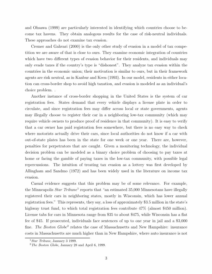
There are three cases shown in Figure 2.4 In case B there is no tax evasion, in case

C everybody evades, and in case A only the rich do. The individual with income level

y = y∗1 is indifferent. If y∗1 = y, there is no tax evasion. According to this proposition,

if in equilibrium there is any tax evasion in a community, it is the rich agents who evade.

This result is analogous to the spatial competition models of Kanbur and Keen (1993) and

Ohsawa (1999), in which individuals with the lowest transportation cost, i.e., those closest

to the border, are the ones more likely to evade.

The cut-off income level, y∗1, satisfies the following:

Proposition 2 y∗1 is non increasing in T1 and non decreasing in T2.

4Given that u′ > 0, by the inverse function theorem, u−1 exists and is differentiable, thus c is continuousand differentiable in y.

6

Figure 2: Evasion Decisions

�

�

T1

T

y − c(y)

y y yy∗1Case A: The Rich Evade

�

�

T1

T

y − c(y)

y y y

Case B: Nobody Evades

�

�

T1

T

y − c(y)

y y y

Case C: Everybody Evades

Proof. It is enough to prove the result for an interior y∗1 ∈ (y, y). In this case, the implicit

function theorem implies that y∗1 is continuous and differentiable, and we have

∂y∗1∂T1

=u′(y∗1 − T1)

u′(y∗1 − T1) − (1 − π)u′(y∗1 − T2) − πu′(y∗1 − T2 − F )< 0.

The sign follows because the numerator is positive and the denominator is negative by lemma

1 in the appendix. We can show that∂y∗

1

∂T2> 0 in the same manner. An analogous result can

be established for y∗2.

Figure 3: Characterization of y∗1

�

�

y∗1

y

y

T1

�

�

y∗1

y

y

T2

Intuitively, when the tax difference is larger, poorer agents can afford to take the risk of

evading. If the gains from evasion are small, only the richest people will be able to afford

choosing the implied lottery of tax evasion. See Figure 3. Clearly, if taxes coincide there is

no incentive to evade.

7

2.2 Game Between Local Governments

Local governments set their taxes strategically in a two-stage game. In the first stage, they

announce their policies; in the second stage, individual decisions on tax evasion determine

the tax base in each community.

The solution concept is subgame perfection. An equilibrium is characterized by backward

induction replacing the decision rules of individuals—represented by cut-off levels of income

y∗i —in the objective functions of the local governments. The values y∗i determine who evades

taxation in each location. The tax base is formed by local agents who do not evade and

foreign agents who evade in their community of origin. In addition, fines are collected from

local agents who evade and are caught; by the law of large numbers, they represent a fraction

π of tax evaders.

The revenue function of local government 1 is given by the following expression:

R1 (T1, T2) =

{{N1 +N2[1 − Φ(y∗2)]}T1 if T1 ≤ T2

N1Φ(y∗1)T1 +N1[1 − Φ(y∗1)]πF if T1 ≥ T2,(2.2)

where Φ(y∗i ) is the fraction of individuals that evade taxes in community i.

Definition 1 A pure strategy equilibrium for this environment is a tax for each community,

(T1, T2) cut-off income levels, y∗1 and y∗2, such that:

i) Ti solves the problem of community i given the policy of the other community, Tj, for

i, j = 1, 2, i �= j, and aggregate decision rules, summarized by cut-off levels y∗1 and y∗2,

ii) income levels y∗1 and y∗2 are determined consistently with individual decision problems

when residents take policies (T1, T2) as given.

The above definition of equilibrium corresponds to the Nash equilibrium of the reduced

game defined by incorporating agents’ best responses to announced governments’ policies in

the payoff functions of the local governments: ΓN = [I, {Si} , {Ri}] , where I = {1, 2} is the

set of communities or local governments; Si =[0, T

] ⊂ � is the set of strategies for local

government i, and Ri is the payoff defined in equation (2.2).5 It is easy to see that the payoff

functions in our problem need not be concave because of the endogenous determination of the

tax base. In such cases, there are no general results guaranteeing existence of pure strategy

equilibria. However, mixed strategy equilibria are shown to exist in Glicksberg (1952) under

continuity of the payoff functions alone.6 In what follows we will examine properties of pure

5Notice that given the structure of the model, in order to guarantee non-negativity of net income for thelowest income type, we have to define a maximal tax T < y.

6In our case, the objective function Ri is continuous if the cut-off levels y∗i are continuous and the income

distribution function has no mass points. In the appendix we show y∗i is continuous.

8

strategy equilibria when they exist, in particular, the way policies determine the mobility of

the tax base through the tax evasion decisions of individuals.

3 Size Effects on Policies

In the model, communities may differ only in the size dimension. In this section, we ask

whether small communities set lower taxes in equilibrium. In order to examine the effects

of differences in community size, we allow for differences in total mass, Ni. It turns out

that having a smaller population allows locations to gain by undercutting the rival’s tax rate

and attracting a large mass of evaders. The large location, in contrast, has more to lose by

attempting to undercut the smaller rival because of its own large base.

3.1 Identical communities: N1 = N2

With identical communities we could imagine that an asymmetric situation could be an

equilibrium: for example, one community sets lower taxes and attracts the top portion of

the population of the rival community, which sets a higher tax on its reduced base. But

this intuition is not correct, as shown in proposition 3: with equally sized communities there

cannot be an asymmetric equilibrium in pure strategies.

Proposition 3 If N1 = N2 = N, then in any equilibrium (T1, T2), T1 = T2.

Proof. Suppose there is an equilibrium with T1 �= T2. Without loss of generality, let

T1 > T2. Lemma 2 in the appendix then implies that T1 − T2 > πF . Since (T1, T2) is an

equilibrium, we must have

R1(T1, T2) ≥ R1(T2, T2)

R2(T1, T2) ≥ R2(T1, T1).

Adding these inequalities we obtain

NΦ(y∗1)T1+N(1−Φ(y∗1))πF+NT2+N(1−Φ(y∗1))T2 ≥ NT2+NT1,

which is equivalent to

−(1−Φ(y∗1))(T1−T2) ≥ −(1−Φ(y∗1))πF.

9

Notice that (1 − Φ(y∗1)) > 0, i.e., there is some evasion, otherwise, by the same argument

as in lemma 2, it would pay jurisdiction 2 to raise its tax rate. Then T1 − T2 ≤ πF , a

contradiction.

It turns out that the only possibility for equilibrium in pure strategies with identical

communities is the one in which governments set maximal taxes, as implied by the next

result.

Proposition 4 Assume F > 0 and π > 0. If there exists a symmetric equilibrium in pure

strategies, (T, T ) , it must be that T = T .

Proof. Suppose (T, T ) is an equilibrium and T < T . In this situation there is no evasion,

since, for any agent with income y in either community,

u(y−T ) > (1−π)u(y−T )+πu(y−T −F ).

Because the inequality is strict, either community can slightly increase its tax without induc-

ing any evasion and increase its revenue. Therefore (T, T ) could not have been an equilibrium.

The difficulty in finding equilibria where tax rates are not maximal lies in the assumption

that all individuals must pay taxes. If local governments allowed individuals for whom net

income became negative to be exempt from taxation, it might then be possible to find pure

strategy equilibria where taxes fall below the highest income level. This extension would

require using exceptional qualifications for tax evaders, for example, when an individual is

only constrained if he gets caught.

3.2 Different communities: N1 > N2

Casual evidence suggests that larger (or more densely populated) communities tend to

set higher taxes. Smaller communities, by fixing a lower tax, can generate extra revenue

collected from tax evaders attracted from the rival community—at the cost of losing revenue

from the local population. Intuitively, small communities have more to gain from attracting

a larger mass of tax evaders, because the density of their own tax base is small. In our model

when community sizes differ, the larger community does not set the lower tax.

Theorem 1 When locations differ in size, the smaller community will set the smaller tax

rate, i.e., (N1 −N2)(T1 − T2) > 0.

10

Proof. Let θ = N1/N2. Without loss of generality, let T1 > T2.

In equilibrium we must have,

R1(T1, T2) ≥ R1(T2, T2) (3.1)

R2(T2, T1) ≥ R2(T1, T1).

Expanding we can express these inequalities as

θT1Φ(y∗1) + πFθ[1 − Φ(y∗1)] ≥ θT2

T2 + T2θ[1 − Φ(y∗1)] ≥ T1.

Adding the expressions and manipulating we obtain:

(θ−1)(T1−T2) ≥ (T1−T2−πF )θ[1−Φ(y∗1)]. (3.2)

The argument in lemma 2 implies that when T1 �= T2, in equilibrium we must have |T1−T2| >πF , it also implies that there is some evasion, i.e., (1 − Φ(y∗1)) > 0, and therefore the result

follows.

The smaller jurisdiction therefore has strong incentives to undercut its larger rival’s rate

to induce evasion in that community. Intuitively, in order to sustain evasion in equilibrium,

the difference in tax rates has to exceed the expected payment of fines.

An interesting question that arises is whether a similar result can be established if instead

of examining large and small communities, we looked at rich vs. poor jurisdiction, as it is

often done when analyzing population migration models in the spirit of Tiebout (1956). It

turns out that examining the effects of differences in income distribution, normalizing N1 =

N2 = 1 and allowing the density functions, φi, to vary, does not yield a clear characterization,

as in the case of size differences. If we define community 1 to be richer than community 2

when Φ1(x) ≤ Φ2(x) for all x ∈ [y, y], there are two opposing effects. Taking the tax rate of

the rich community as given, the poor community by fixing a lower tax can attract the top

portion of the rich community—a stealing effect—but it can also set a higher tax to increase

local revenues, knowing that its local agents will probably not take the chances of evasion—a

capturing effect. In general, it is not possible to determine which effect dominates.7

7For example, let community 1 have a degenerate distribution at some income level, y1, then it has tobe that T1 ≤ T2. In an equilibrium with T1 > T2 there cannot be any tax evasion in community 1. Thereason is that since all individuals are identical, tax evasion would imply that everyone evades and revenuesare zero. The government in community 1 could then increase revenues by setting the same tax as therival community. Now, because there is no evasion in community 1, R2(T1, T2) = T2 < R2(T1, T1) = T1, acontradiction.

11

4 Tax Harmonization

In this section we are interested in the possibility and the effects of tax harmonization.

In a strict sense our analysis is not a welfare analysis since we will focus only on fiscal

revenue. We want to know (1) whether it is possible (in the sense of individual rationality)

to implement a harmonization policy over taxes, (2) under what conditions would this be

possible, and (3) how would this affect revenue collection in both communities.

4.1 Harmonization with Transfers

First we restrict our analysis to the possible joint revenue gains from harmonization to a

common tax rate, T h, without discussing for the moment the incentives of each community

to deviate from the agreement. We can think of this harmonization scheme as imposed by

a federal government with the local governments forced to compel or as an agreement with

transfers between communities.

Let (T1, T2) be an equilibrium for N1 > N2. Let T h be the harmonized common tax rate.

To facilitate exposition we will abbreviate notation in the following way:

Ri = Ri (T1, T2)

Rhi = NiT

h

Φ = Φ(y∗1)

θ =N1

N2.

Therefore,

R1 = N1ΦT1 +N1 (1 − Φ) πF

R2 = N2T2 +N1 (1 − Φ)T2.

It is not obvious that a harmonized common tax rate will lead to maximal joint revenues

since it may be optimal (for a joint revenue maximizer) to allow some evasion with differen-

tiated tax rates, given that there is a percentage π of all evaders that end up paying the tax

rate of one community plus the fine of the other.

It turns out that if transfers can be implemented between communities, there is always

a minimum common tax rate such that both communities benefit from harmonization and

it is intermediate to the tax rates in the non-cooperative equilibrium.

Note that we made no assumption on the income level of community 1. In particular the example holdsif y1 = y2 or y1 = y2.

12

Proposition 5 Let T ≡ ΦT1 + (1 − Φ) (T2 + πF ), then communities will benefit from har-

monization if and only if T h ≥ ωT + (1 − ω)T2, where ω ≡ θ1+θ

.

Proof. Note that

R1 +R2 = N1ΦT1 +N1 (1 − Φ) (T2 + πF ) +N2T2

Rh1 +Rh

2 = N1Th +N2T

h.

Then Rh1 + Rh

2 ≥ R1 + R2 if and only if N1Φ(T h − T1

)+ N1 (1 − Φ)

(T h − T2 − πF

)+

N2

(T h − T2

) ≥ 0. Since T1 > T2 + πF , again by lemma 2, a necessary condition is T h > T2;

then simply solving for T h gives the desired condition.

It is interesting that the minimum harmonization tax rate required to guarantee larger

joint revenues than those in the non-cooperative equilibrium is strictly between the two

non-cooperative tax rates. The reason is that coordinating to an intermediate tax rate may

be politically more feasible than imposing the maximal tax rate, T , which would obviously

maximize joint revenues subject to the constraint of requiring a common tax rate. If an in-

termediate tax rate is chosen, however, we will see that community 2 has to be compensated.

4.2 Harmonization without Transfers

If transfers between communities cannot be implemented, possibly because they are costly

in terms of coordination or because the political implications are not desirable for the local

governments, in order for jurisdictions to agree on harmonizing policies, individual revenues

need to improve for both locations. In this subsection we do not present a theory of why

this happens, we take this fact as given and provide conditions under which harmonization

is beneficial or harmful to communities when side transfers are not allowed. Thus we impose

that each community has to be at least as well off with the harmonized tax than in the non-

cooperative equilibrium. This harmonized taxation may be the result of explicit negotiations

between communities or we can think of it as an implicit collusion outcome of the game played

repeatedly over infinite periods with a sufficiently high discount factor.8

Proposition 6

a) Neither community benefits from a harmonized tax rate lower than the smaller commu-

nity’s non-cooperative tax rate.

b) If (T1, T2) is an equilibrium with T2 < T1, the smaller jurisdiction never benefits from a

harmonization scheme that sets a common tax rate T h with T2 ≤ T h ≤ T1.

8In the short run communities have an incentive to deviate. Therefore harmonized taxation is a subgameperfect Nash equilibrium only if the present value of future losses from not cooperating today is high enough.

13

Proof. a) The smaller jurisdiction does not benefit since it will not collect taxes from

evaders and it is collecting lower taxes from its own residents. With respect to the larger

jurisdiction, note that for T h < T2 it is the case that

R1 (T1, T2) ≥ R (T2, T2) = N1T2 ≥ N1Th,

where the first inequality follows from T1 being a best response to jurisdiction 2 fixing a tax

rate of T2. Therefore the larger community does not benefit from taxes below T2 either.

b) If we harmonize to the larger tax rate, T h = T1, then clearly,

R2(T1, T2) ≥ R2(T1, T1) = N2T1,

because T2 is a best response to T1. If we harmonize to the smaller tax rate, then

R2(T1, T2) = N2T2+N1 (1 − Φ)T2 > N2T2 = R2(T2, T2).

Now, if we harmonize to an intermediate tax rate, T h,

R2(T1, T2) ≥ R2(T1, T1) = N2T1 ≥ N2Th = R2(T

h, T h).

This result is analogous to proposition 9 in Kanbur and Keen (1993), where a similar

problem is analyzed with risk-neutral individuals. We now give conditions under which

harmonization would garner benefits for both communities.

Proposition 7 If there can be no transfers between jurisdictions, communities can benefit

from harmonization if and only if

T h > max{T2 (1 + (1 − Φ) θ) , T1}.

Proof. We need the fiscal revenues of each community in the harmonized scheme to be

larger than in the non-cooperative case. Consider first the small community: Rh2 > R2 if

and only if

N2Th > N2T2 +N1 (1 − Φ)T2.

But by proposition 6, the smaller jurisdiction will not benefit if the harmonized tax rate is

not greater than T1, therefore the stated condition must hold. The larger community will

14

also benefit, since Rh1 > R1 if

N1Th > N1ΦT1 +N1 (1 − Φ) πF ,

and by lemma 2 in the appendix this holds since T1 > T1 − T2 > πF , and therefore T h >

T1 = ΦT1 + (1 − Φ)T1 > ΦT1 + (1 − Φ) πF .

The larger jurisdiction would benefit from harmonization with a tax rate even smaller

than T1 since evasion would be prevented in the harmonized environment. The necessary

condition for the larger community to benefit from a harmonized tax rate is

T h ≥ T1 − [1−Φ][T1 −πF ],

but a common tax rate equal to the right-hand side would harm the smaller jurisdiction.

The premium the small jurisdiction has to receive in terms of a higher common tax rate

is proportional to the fraction of evaders from the large location in the non-cooperative

equilibrium. Therefore whenever the smaller community agrees to harmonize taxes, the

larger one will as well.

5 Optimal Monitoring

In this section we consider situations in which communities have already committed to

a tax policy and now have to choose optimal monitoring, which is costly.

Monitoring determines the risk that individuals face in the case of evasion. In our previous

environment, when a given monitoring policy is less stringent, communities face a more elastic

tax base, which implies tougher competition. Local governments respond by lowering taxes

to reduce the incentives to evade. In the extreme case of no monitoring effort, undercutting

may lead to cut-throat competition. Intuitively, if either the (fixed) probability of getting

caught or the penalties are equal to zero across locations, whenever taxes differed, everyone

in the high-tax location would choose to evade. Thus in equilibrium taxes would have to be

equal because the tax base is perfectly mobile. Undercutting—in a Bertrand competition

spirit—then would drive tax rates to zero. Revenue collection in such a case would be zero

in each community.

In what follows we assume that the probability of getting caught is a policy instrument

for the local communities, given now fixed tax policies across locations.9 We also assume

9In the 1998 agreement between communities in Uruguay, taxes were fixed for each location and the onlyvariable still under the control of local governments was their monitoring effort.

15

there is a per capita cost of monitoring, given by an increasing function m (π).

We assume T1 > T2 and T1 < T2 +F so that it is possible to induce at least some agents

not to evade. Clearly, community 2 will not monitor because it has the lower tax, so the

focus is on community 1.

5.1 Homogenous Monitoring

Suppose local governments are not able to set different levels of monitoring in terms of

income level. In this situation, given the fixed tax rates in each community, local revenues

as a function of the monitoring probability are given by

R1 (π;T1, T2) = N1Φ(y∗1(π;T1, T2))T1+πFN1[1−Φ(y∗1(π;T1, T2))]−N1m(π). (5.1)

The optimal level of monitoring is characterized by the following first-order condition:

[T1 − πF ]φ(y∗1(π;T1, T2))∂y∗

∂π+F [1−Φ(y∗1(π;T1, T2))] =

∂m(π)

∂π, (5.2)

where the response of the cut-off level, y∗1, to changes in the probability of being caught is

∂y∗1∂π

=u(y∗1 − T2 − F ) − u(y∗1 − T2)

u′(y∗1 − T1) − (1 − π)u′(y∗1 − T2) − πu′(y∗1 − T2 − F )< 0. (5.3)

The left-hand side in (5.2) shows the marginal benefit of increasing the level of monitoring.

The first term indicates the net marginal gain from having evaders pay taxes instead of fines,

and the second term is the increase in fines collected from perpetrators that are now more

likely to get caught. The right-hand side represents the marginal cost of increasing the level

of monitoring.

The next example illustrates the case of a high-tax community optimally choosing a

constant monitoring policy. As would be expected, it is optimal for this community to allow

some level of evasion. In Figure 4 we show the revenues as a function of the audit probability

π.

• N1 = N2 = 1

• φ1(y) = φ2(y) =(

yy

y−y

)y

y2 with y = 10 and y = 150

• u(y) = 1b−1

(a+ by)1− 1b , a = 2, b = 0.2

• m(π) = 10 π(1−π)

16

Figure 4: Optimal homogeneous monitoring

-2

-1.5

-1

-0.5

0

0.5

1

1.5

2

2.5

0 0.05 0.1 0.15 0.2 0.25 0.3 0.35 0.4

Prob. of getting caught

Rev

enu

e

• F = 6, T1 = 5, T2 = 3.5

In this community, the optimal monitoring policy, π = 0.2208, results in an income cut-

off value of y∗1 = 89.54. Given the Pareto distributions we assumed, this implies that the top

4.82% of agents in community 1 decide to evade taxation.

5.2 Differentiated Monitoring

It is desirable to analyze the possibility of having monitoring depend on income levels. If

it were possible to implement such a policy, it is clear that there would have to be a positive

level of monitoring for all income levels in the high-tax community, since otherwise whoever

is not monitored will evade. To get some intuition, consider initially a fixed monitoring

policy, π, which results in an interior cut-off income level, y∗1. The local government may

increase net revenues by changing to a variable monitoring policy, π(y). A variable policy

would allow the government to lower costs of monitoring agents with income levels below y∗1,

without inducing them to evade, but it would be costly to induce agents with incomes above

y∗1 not to evade. The optimal monitoring policy for each income level in this environment is

obtained comparing the net benefits of collecting taxes or expected fines for each individual.

Intuitively, there may exist an income level y1 such that it does not pay community 1 to

prevent agents with y ≥ y from evading. The local government should set a monitoring

policy for these agents who evade so as to maximize expected revenue from fines.

In the region of income levels where the government induces compliance, it will maximize

the difference between tax and monitoring costs per individual, subject to inducing agents

to pay taxes at home. The optimal policy in this region is obtained with a constrained cost

minimization problem.

17

In the region of income levels where the government allows evasion and collects fines,

it will maximize the difference between fines and costs of monitoring agents who choose to

evade.

We show in the following paragraphs that in the region of compliance the net benefit

from collecting taxes, T −m(πT (y)), is decreasing in y. In the region of tax avoidance, the

monitoring policy of evaders, πF , will not depend on income, and the net benefit will be

constant.

Proposition 8 There exists a cut-off level of income, y, such that the optimal monitoring

policy for community 1 takes the following form:

π(y) =

{πT (y) = u(y−T2)−u(y−T1)

u(y−T2)−u(y−T2−F )if y < y

πF = m′−1(F ) if y ≥ y.

Proof.

Step 1. In the compliance region, since monitoring is costly, the local government will not

monitor in excess. The government sets π(y) in this region, such that:

u(y−T1)−(1−πT (y))u(y−T2)−πT (y)u(y−T2−F ) = 0.

Thus

πT (y) =u(y − T2) − u(y − T1)

u(y − T2) − u(y − T2 − F ).

This expression is increasing in income:

∂πT (y)

∂y=

[u′(y − T2) − u′(y − T1)] [u(y − T2) − u(y − T2 − F )]

[u(y − T2) − u(y − T2 − F )]2

− [u(y − T2) − u(y − T1)] [u′(y − T2) − u′(y − T2 − F )]

[u(y − T2) − u(y − T2 − F )]2

>[u′(y − T2) − u′(y − T1)] [u(y − T2) − u(y − T2 − F )]

[u(y − T2) − u(y − T2 − F )]2

− [u′(y − T2) − u′(y − T2 − F )] [u(y − T2) − u(y − T2 − F )]

[u(y − T2) − u(y − T2 − F )]2

=[u′(y − T2 − F ) − u′(y − T1)] [u(y − T2) − u(y − T2 − F )]

[u(y − T2) − u(y − T2 − F )]2> 0.

18

Step 2. In the avoidance region, the optimal monitoring policy solves

maxπF (y)

N1

∫ y

y

[πF (y)F −m

(πF (y)

)]φ1(y)dy.

The first-order condition,

F = m′ (πF (y)),

implies that πF = m′−1(F ) is constant.

Step 3. In order to find the level y above which the government allows evasion, the following

problem is solved:

max�y

∫�y

y

[T −m(πT (y))

]φ(y)dy+

∫ y

�y

[πFF−m(πF )]φ(y)dy.

The first-order condition is given by

T −m(πT (y)) = πFF −m(πF ).

The left-hand side is the net marginal benefit from compliance, and it is a strictly decreasing

function of y. The right-hand side is the net marginal benefit from expected fines in the

avoidance region, and it is a constant function. The level y is thus uniquely defined.

The determination of the cut-off level, y, is shown in Figure 5.

Figure 5: Determination of y

�

�

T1 −m(πT (y))

πFF −m(πF )

y y

Given that the large community’s tax rate, T1, is not guaranteed to be equal to the

term πFF , the expected benefit from evaders, the schedule π (y) can admit discontinuities

19

at the cut-off level, y, but only in downward jumps, since community 1 could improve by

saving on monitoring costs if πF > πT (y). Also, although we have characterized an interior

solution for the cut-off point, y, it may be optimal to prevent evasion for all income levels if

T1 −m(πT (y)

)> πFF −m

(πF

), and in that case the monitoring schedule would coincide

with πT (y).

6 Conclusion

The model developed in this paper examines tax competition in a framework with

residence-based taxation in which authorities can only imperfectly monitor the origin of

tax payers who may choose to evade local taxation by pretending to be residents of the rival

low-tax community. We characterize the properties of equilibria in pure strategies when

communities differ in size and find that small communities have advantages in capturing

some tax base from their rival by undercutting their higher tax rate.

We also characterize the problem facing individual residents who evaluate the payoffs of

complying with local taxation and the resulting lottery of evasion. Decreasing risk aversion

implies that only high-income agents can afford to choose the evasion lottery. This feature is

comparable to existing modeling strategies in spatial frameworks of cross-border shopping,

where risk-neutral individuals have unit demands and valuation net of costs of transportation

replaces our definition of income.

Our model clearly indicates that integration, in the sense of joint revenue maximization,

can always be beneficial from the perspective of local governments. If communities have a way

to make side transfers between them, then the minimum tax rate required to generate joint

benefits in the harmonization scheme is strictly between the two non-cooperative tax rates.

This is important if coordinating to a different tax rate is more costly. Even without side

transfers, there are potentially important benefits from harmonization when the minimum

agreeable tax rate implies a premium to the small community’s non-cooperative tax rate

proportional to the fraction of tax evaders in the large community.

In our framework, lump-sum tax policies imply that relatively less risk-averse agents can

avoid high taxes by fleeing to another community. This feature makes the head tax structure

regressive. Presumably, a federal authority in charge of choosing an optimal tax structure

superseding fiscal competition would take into account attitudes toward risk in its design.

In an environment where locations have already committed to a set of tax policies and

have to choose monitoring efforts to prevent tax evasion, we show that it may be optimal for

a high-tax community to allow some people to evade and that the audit probability should

be increasing over the compliance region and constant over the avoidance region.

20

The implications of the model seem to be in line with some casual evidence for some

regions of the United States and preliminary evidence for Uruguay that find statistical cor-

relation between community size and the distribution of car values across municipalities, as

well as between size and magnitude of registration fees.

In a more general analysis of policy coordination, particularly between countries, it would

be interesting to study the larger version of the game where both tax and monitoring policies

can be used strategically. Presumably, even when some type of coordination can be achieved

with respect to tax policies, harmonization of monitoring efforts is more costly.

Another question that arises regarding integration of countries is whether allowing for

population migration implies some kind of sorting result. In such a framework, we could

study the different implications of having borders closed to household migration, as we have

done in our model, and opening borders so that individuals who migrate are no longer

considered tax evaders. Traditional models of migration of heterogeneous population obtain

stratification results in terms of income; in an environment with migration costs, individuals

would face the options of evading taxation or emigrating to the low-tax country, and it might

be interesting to examine whether stratification still holds.

Appendix

Define

U(y, T1, T2) = u(y−T1)−(1−π)u(y−T2)−πu(y−T2−F ).

Lemma 1 If (T1, T2) are tax rates such that y∗1 ∈ (y, y

), then ∂U(y,T1,T2)

∂y

∣∣∣y=y∗

1

< 0.

Proof. Note that U(y∗1, T1, T2) = 0 ⇔ y∗1 − c(y∗1, T1, T2) = T1.

The assumption of DARA implies ∂[y−c(y,T1,T2)]∂y

< 0, and therefore ∂c(y,T1,T2)∂y

> 1. From the

definition of c(y, T1, T2), we have u′(c(y, T1, T2))∂c(y,T1,T2)

∂y= (1−π)u′(y−T2)+πu

′(y−T2−F ),

which implies (1 − π)u′(y − T2) + πu′(y − T2 − F ) > u′(c(y, T1, T2)) for all y.

Finally we have:

∂U(y, T1, T2)

∂y

∣∣∣∣y=y∗

1

= u′(y∗1 − T1) − (1 − π)u′(y∗1 − T2) − πu′(y∗1 − T2 − F )

< u′(y∗1 − T1) − u′(c(y∗1, T1, T2)) = 0.

The last equality follows from the definition of c(y, T1, T2) and y∗1 interior.

21

Proposition 9 The cut-off income level, y∗1, defined in equation (2.1) is continuous in

(T1, T2).

Proof. It is enough to show continuity for tax policies (T1, T2) such that y∗1 ∈ (y, y).

Given tax rates (T1, T2), an agent with income y in community 1 decides to evade if U(y, T1, T2) <

0. Since

∂U(y, T1, T2)

∂y

∣∣∣∣y=y∗

1

< 0,

by lemma 1; the implicit function theorem then implies that the function y∗(T1, T2) such

that U (y∗ (T1, T2) , T1, T2) = 0 is continuous in the set of policies (T1, T2).

Lemma 2 If (T1, T2) is an equilibrium with T1 �= T2, then |T1 − T2| > πF .

Proof. Without loss of generality, let T1 > T2. Now suppose there is an equilibrium

(T1, T2) where T1 − T2 ≤ πF . Then T1 − T2 ≤ πF implies that y − T2 − πF ≤ y − T1

for any y in community 1. Rewriting, we have that (1 − π)(y − T2) + π(y − T2 − F ) =

y−T2−πF ≤ y−T1. That is, the expected payoff to evading taxes is less than the payoff to

paying taxes at home, and no one in community 1 would chose to evade since risk aversion

implies u (y − T1) ≥ (1− π)u(y − T2) + πu(y − T2 − F ). Therefore, since R2(T1, T2) = N2T2

and T2 < T1 ≤ T , it would pay community 2 to raise its tax rate T2, and therefore (T1, T2)

could not be an equilibrium.

22

References

[1] Bureau of the Census, U.S. Department of Commerce Economics and Statistics Admin-

istration, 1990, Census of Population and Housing (Washington, D.C.).

[2] Federal Highway Administration, U.S. Department of Transportation, 1990, Highway

Statistics (Washington, D.C.).

[3] Allingham, M. G. and A. Sandmo, 1972, Income Tax Evasion: A Theoretical Analysis,

Journal of Public Economics 1, 323-338.

[4] Beard, T. Randolph, Paula A. Gant and Richard P. Saba, July 1997, Border-Crossings

Sales, Tax Avoidance, and State Tax Policies: An Application to Alcohol, Southern

Economic Journal 64(1), 293-306.

[5] Bucovetsky, S., 1991, Asymmetric Tax Competition, Journal of Urban Economics 30(2),

167-181.

[6] Crawford, Ian and Sarah Tanner, May 1995, Bringing It all Back Home: Alcohol Tax-

ation and Cross-Border Shopping, Fiscal Studies 16(2), 94-114.

[7] Cremer, Helmuth and Firouz Gahvari, 2000, Tax evasion, fiscal competition and eco-

nomic integration, European Economic Review 44(9), 1633-1657.

[8] Glicksberg, I. L., February 1952, A Further Generalization of the Kakutani Fixed Point

Theorem, with Application to Nash Equilibrium Points, Proceedings of the American

Mathematical Society 3(1), 170-174.

[9] Gordon, Roger H. and Soren Bo Nielsen, 1997, Tax Evasion in an Open Economy: Value

Added vs. Income Taxation, Journal of Public Economics 66(2), 173-197.

[10] Kanbur, Ravi and Michael Keen, September 1993, Jeux Sans Frontieres: Tax Competi-

tion and Tax Coordination When Countries Differ in Size, American Economic Review

83(4), 877-892.

[11] Ohsawa, Yoshiaki, 1999, Cross-Border Shopping and Commodity Tax Competition

Among Governments, Regional Science and Urban Economics 29(1), 33-51.

[12] Saba, Richard P., T. Randolph Beard, Robert B. Ekelud, Jr., and Rand Ressler, April

1995, The Demand for Cigarette Smuggling, Economic Inquiry XXXIII(2), 189-202.

23

[13] Tiebout, Charles M., 1956, A Pure Theory of Local Expenditures, Journal of Political

Economy 64(5), 416-424.

[14] Wilson, J. D., 1986, A Theory of Interregional Tax Competition, Journal of Urban

Economics 19, 296-315.

[15] Wilson, J. D., 1991, Tax Competition with Interregional Differences in Factor Endow-

ments, Regional Science and Urban Economics 21, 243-451.

24