task 6 - safety review and licensing on the job training...

Task 6 - Safety Review and LicensingOn the Job Training on Stress Analysis

Pisa (Italy)June 15 – July 14, 2015

Static strength and High and Low-Cycle Fatigueat room temperature 2/2

Davide Mazzini – Ciro Santus

2

Content

• Fatigue of metals

- Definitions

- Different approaches to fatigue, Stress/ Strain life

- Low/ High Cycle Fatigue

- Fatigue notch sensitivity

Table of content – Class VI.a.2

Pisa, June 15 – July 14, 2015

3

Books on Metal fatigue

S. Suresh. Fatigue of Materials. Cambridge University Press 1998.

H. E. Boyer. Atlas of Fatigue Curves. ASM International 2003.

R. I. Stephens, A. Fatemi, R. R. Stephens, H. O. Fuchs . Metal Fatigue in

Engineering. Wiley 2001.

… and many many others

Books


4

Cyclic load leading to fracture

Fatigue - Intro

Cyclic loading, repeatedthousands or even millions of times

EventualFatigue Fracture


5

Nucleation

Persistent Slip Bands, PSBs

Fatigue – Evolution of the crack

These slip lines were termed 'persistent slip bands' (PSBs) by Thompson, Wadsworth & Louat (1956) who found that in Cu and Ni, the bands persistently reappeared at the same sites during continued cycling even after a thin layer of the surface containing these bands was removed by electropolishing.


6

Nucleation

“Embryo” crack formation from PSBs


Irreversibility of the cyclic slip


7

Nucleation

“Embryo” crack formation from PSBs



8

Stage I – Stage II

Forsyth ~1960


Stage I: propagation at 45°, single path or “zig-zag”, within a single grain (or very few grains)

Single slip system


9

Stage I – Stage II

Forsyth ~1960


Stage II: perpendicular propagation on many grains

Two slip systems


10

Stage II propagation and striations (beachmarks)



11

Stage I usually at Inclusions (or other defects) in commercial metals


Even subsurface nucleation


12

Different possible

nucleation scenarios



13

Stage III is the final fracture, so called “Sudden” or “Unstable”


This can be considered a static fracture…


14

Nucleation/ Propagation

What is the transition point from Nucleation to Propagation?

Stage I to Stage II

1 mm

It does not matter

It depends on the inspection method

Number of cycles, N110 210 310 410 510 610 810

Crack size,a Load amplitude

?


15

Nucleation/ Propagation

Nucleation to Propagation percentage of the entire fatigue life

No crack evolution below the Fatigue LimitDesign value

Number of cycles, N110 210 310 410 510 610 810

Crack size,a Load amplitude

?


16

Fatigue – Engineering viewpoint

Engineering approaches

Stress life (High Cycle Fatigue – HCF)

Strain life (Low Cycle Fatigue – LCF)

Fracture Mechanics (Damage Tolerant Design)


17

Definitions

Stress life approach

Amplitude and mean stresses


18

Definitions


min

max

Load ratio:

Ex.:Alternate load: (default for testing)

0Repeated l

1

oad:

R

R

R

Time

Time


19

S-N curves – Testing machines (historical)


Moore rotating bending machine4-pont bending load scheme

Homework:

Find the load cycle experiencedat the mid section of the specimen,depending on the weight and sizes of the specimen


20

S-N curves – Testing machines


Resonance basedPush-pull fatigue testing machine100-150 HzEx.: RUMUL

Hourglassspecimen

Very blunt notch,Equivalent to a plain specimen


21

Specimen shape for fatigue testing


Stressconcentration---Why is this not a problem for the Tensile Test?

Hourglassspecimen

Very blunt notch,Equivalent to a plain specimen

Gauge lengthnot required


22

S-N curves, or Wöhler curve


a

Alternatestress, σ

Each point is a specimenSeveral points at single load levelSome load levels

Runouts:Specimens not broken,Test stopped at a specified maximum number of cyclesEx.: 10 millions (107)

Fit line, or S-N curve

Log scale !!!

Either Log or linear scale


23

Endurance limit, only for steels


Fatigue strength at 105

Fatigue strength at 108


24

Standard ISO 12107

How many specimens are required?

15 tests (minimum)


25

Number of cycle/ Stress scatter

Large scatter of fatigue

Very uncertain design values, especially in terms of Finite life Number of cycles to failure


26

Design curve

Large scatter of fatigue

Fit line, 50% reliability

Design curve,higher reliability,ex.: 99%, or even 99.9 %

Standard deviation


27

Testing procedure for Fatigue Endurance

The Staircase method

Numerical procedure to calculate Mean and Standard Deviation

Number of required specimens: 15-20


28

Different regions of the S-N curve

Low Cycle/ High Cycle Fatigue

Fatigue Endurance/Ultra-High Cycle Fatigue (UHCF)

1 cycle = Tensile Test

LCFElastic-plastic cyclic loading

HCFElasticcyclic loading


29

S-N curve values for Steels

Low Cycle/ High Cycle Fatigue

Fatigue Endurance

f a U3

f a U

6f

a S G R U

S

G

R

1

1,

10 , 0.9

10 ,0.5

: Surface factor: Gradient factor: Reliability factor

R

N S

N S

NC C C S

CCC

US

U0.9 S

n S G R U0.5S C C C S


30

Basquin’s law (HCF)

High Cycle Fatigue

FatigueEndurance

a f f

a f

1

a f

Different forms,samelaw:(2 )

( )

( )1/

, are material properties

b

b

k

N

a N

a Nk b

a b


31

Basquin’s law (HCF)

High Cycle Fatigue

a f( )ba N

Exercise:

Find the a, b parameters for the Steel HCF line as function of the Ultimate Tensile Strength and the correcting factors CX

FatigueEndurance


32

LCF requires the Strain life approach

Low Cycle Fatigue

LCF, Elastic-plastic cyclic loading:Limited Stress sensitivityRemarkable Strain variation

FatigueEndurance

a

a

22


33Pisa, June 15 – July 14, 2015

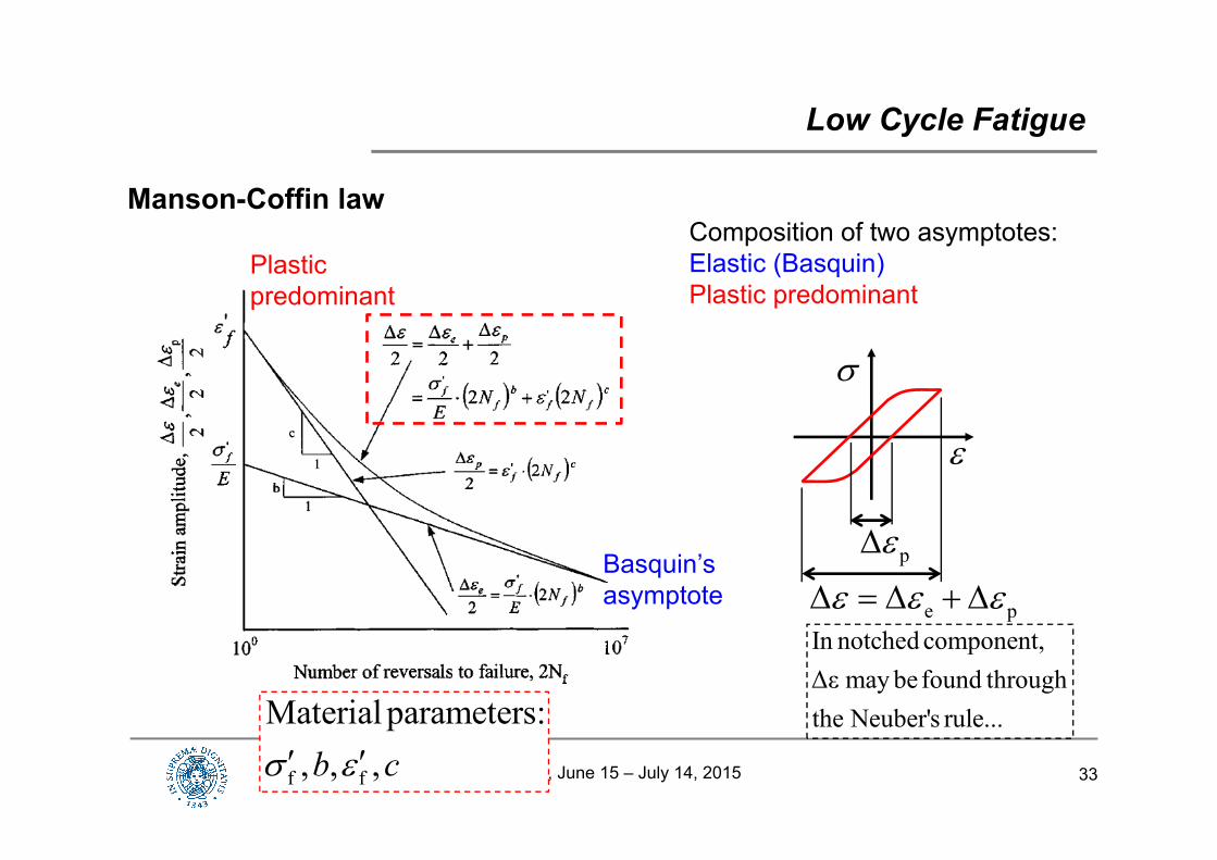
Manson-Coffin law

Low Cycle Fatigue

Composition of two asymptotes:Elastic (Basquin)Plastic predominant

e p

pBasquin’sasymptote

Plasticpredominant

f f

Material parameters:, , ,b c

In notched component,Δε may befound throughthe Neuber's rule...

34

Mean stress effect, different models

High Cycle Fatigue

Higher mean stress, same alternate

Haigh’s diagram


35

Goodman’s line

High Cycle Fatigue

“Modified” Goodman’s line

Values from S-Ncurve at R = -1


36

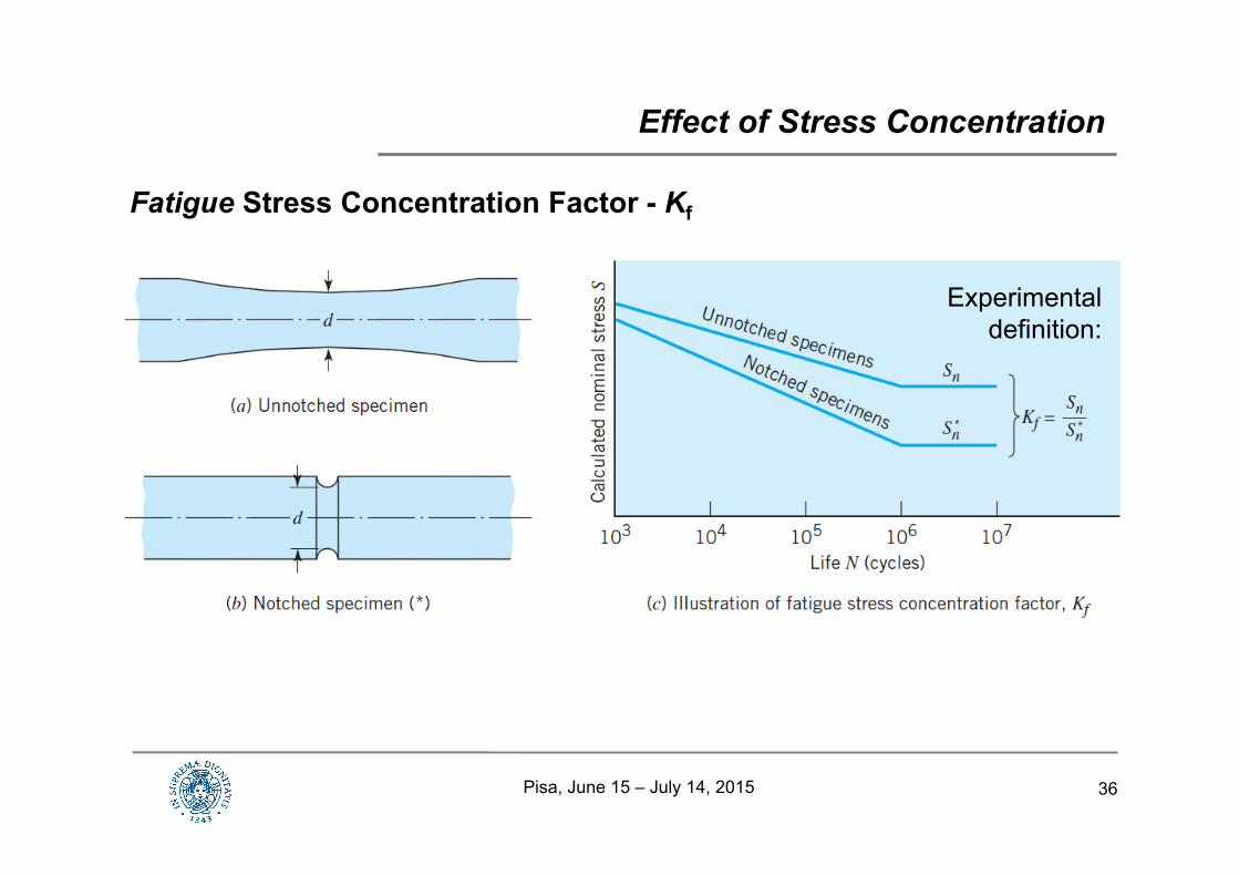
Fatigue Stress Concentration Factor - Kf

Effect of Stress Concentration

Experimental definition:


37

Kf < Kt


*n t n

In fact, fortunately:/S K S

n t/S KExpectedtrend

Same stress at the surface, apparently equal fatigue load


38

Why Kf < Kt ?

Process zone concept



39

How to calculate Kf

The notch sensitivity factor


f

t

f t

11

1 ( 1)

KqK

K q K

q ranges from 0 to 1 and it depends on the Notch radiusand on the material strength (Ultimate Tensile Strength)


40

Numerical example

Calculate the margin with respect to the fatigue endurance

Step 1:

Calculate the material fatigue limit

S

G

R

Un S G R

0.70.80.814

228MPa2

CCC

SS C C C

R.C. Juvinall, K.M. Marshek, Fundamentals of Machine Component Design - Wiley 2011

30 mmd

35mmD

300 NF

Rotating shaftAISI 4340,SU = 1000 MPa

270 mmL

1mmr


41

Numerical example


Step 2:

Calculate the bending nominal stress3

3 3

n

81 10 N mm 81.0 N m

2.65 10 mm32

31MPa

M FL

W d

MW

30 mmd

35mmD

300 NF


270 mmL

1mmr


42

Numerical example


Step 3:

Calculate the Stress Concentration Factor

t

0.033

1.167

2.15

rdD

K

d

30 mmd

35mmD

300 NF


270 mmL

1mmr



43

Numerical example


Step 4:Calculate the Fatigue St. Conc. Factor

U

f

t

Bhn 290 (Brinell)3

0.85.45

(1.

1)98

1

q

S

Kq K

30 mmd

35mmD

300 NF


270 mmL

1mmr



44

Numerical example


Step 5:

Calculate the Safety Factor

n

n f

SF 3.8

SF 1, Ok!

SK

30 mmd

35mmD

300 NF


270 mmL

1mmr


45

Singularity for vanishingly small radius

0r

tK

0q

f t( 0) ( ) ?K q K


46

Singularity for vanishingly small radius

f

The limiting ( 0)value for , is finite,but how tocalculate?

rK


task 6 - safety review and licensing on the job training...

Documents